Influence of gear surface roughness, lubricant viscosity and quality ...

THE INFLUENCE OF SURFACE ROUGHNESS IN
THE TRANSITIONAL FLOW REGIME
MSC 422 – Final Report
Marilize Everts s29037078 Study Leader: Prof J.P. Meyer
2012

MECHANICAL AND AERONAUTICAL ENGINEERING
MEGANIESE EN LUGVAARTKUNDIGE INGENIEURSWESE
INDIVIDUAL ASSIGNMENT COVER PAGE /INDIVIDUELE OPDRAG DEKBLAD
Name of Student / Naam van Student
Student number / Studentenommer
Name of Module / Naam van Module
Module Code / Modulekode
Name of Lecturer / Naam van Dosent
Date of Submission / Datum van Inhandiging
Declaration:
1. I understand what plagiarism is and am aware of
the University’s policy in this regard.
2. I declare that this ____________________ (e.g.
essay, report, project, assignment, dissertation,
thesis, etc.) is my own, original work.
3. I did not refer to work of current or previous
students, memoranda, solution manuals or any other
material containing complete or partial solutions to
this assignment.
4. Where other people’s work has been used (either
from a printed source, Internet, or any other source),
this has been properly acknowledged and referenced.
5. I have not allowed anyone to copy my assignment.
Verklaring:
1. Ek begryp wat plagiaat is en is bewus van die
Universiteitsbeleid in hierdie verband.
2. Ek verklaar dat hierdie __________________ (bv.
opstel, verslag, projek, werkstuk, verhandeling,
proefskrif, ens.) my eie, oorspronklike werk is.
3. Ek het nie gebruik gemaak van huidige of vorige
studente se werk, memoranda, antwoord-bundels of
enige ander materiaal wat volledige of gedeeltelike
oplossings van hierdie werkstuk bevat nie.
4. In gevalle waar iemand anders se werk gebruik is
(hetsy uit ´n gedrukte bron, die Internet, of enige
ander bron), is dit behoorlik erken en die korrekte
verwysings is gebruik.
5. Ek het niemand toegelaat om my werkopdrag te
kopieër nie.
Signature of Student / Handtekening van
Student
Mark awarded / Punt toegeken

Appendix B
REPORT CARD FOR THESIS MSC 412 and 422 20.!:z: .
Name ..m.w.i.\i.~L.f~0.~~...................Reg. no .. ?:-~P.}].Q.7."l>. .
Topic P.~~.~~~.~.J~~j~~~c;n~e. ..<?~.A~.~~.e ~P~~~.~.f,H..i-:,.. ~r.t..~.0.~~H:foY)cM f1vw r-~ime
Leader ..~:.~~..J.f. ..t0.~~ .
Commencement date:.!P.ll~.~}:'-.c?I.. .
Date Par Par Comments
Mf A~
ffl f)~ .re ~
e:~/
/'.<
tt
Registration for Thesis MSC 412 and 422
Name .f0~d~.h,~ Reg. no ..?:-~.~.?!P..~.~ .
Address .~.~!..~~~y~..~t~J ..~Q(~~l:I .. ~P:!~.J.O'9.4~ .
Topic .P~~mi>:'~..~~ ..i~"~en(t ..~ ..~~.~~~..r.t?~.~,V)w..I~..t~ ..t~~Jj~~·~.~~..flow >'T~iWle
Study Leader .p.~~.~.JP. ..~~~ .

REPORT CARD FOR THESIS MSC 412 and 422 20~l,. .
Name..~Q.d\i~~ ~~.0.b..................... Reg. no.. ~~.Q.~]0?~ .
Topic .1h~...\.>:'\\~~.{.~..r!r. )~h~~~.f.~~a~.~.~»..\~.~~..~~~iPp.>:'.':'!..~h>.~.~8 i~
Leader .f~~+..~r.~v .Commencement date:.'?!? !~:.?~.-:.?I .
Date Par Par Comments
3cJ,~h- »<jf}J./l ~fl p..41/../ww
5I'IhIZ Gv IJ Wit P~~M\~
(~/1/'J.I1l-..<--
~
~~-AP~.!'1/~b.h...j ~~.J)
':/;'h ~ 'Ifill rVJ.J,..()l. ~D.. T'I
.,jl;()/~ts: { /1 'J .~f~~~~;" lej'Jt?MI-V"/,/'
"- i--" \ '- I

ABSTRACT
Title: The Influence of Surface Roughness in the Transitional Flow Regime
Author: M. Everts
Student number: 29037078
Study Leader: Prof J.P. Meyer
Commencement Date: 2012-03-01
Completion Date: 2012-10-19
Heat exchangers are usually designed that they do not operate in the transitional flow regime,
mainly due to the uncertainty and perceived chaotic flow behavior and instabilities in this
region. However, due to changes in operating conditions and design constraints, heat
exchangers are often required to operate in this region. Although much research has been
devoted to flow in the transitional flow regime, little information is available on the influence of
surface roughness in this flow regime. Thus, the aim of this study was to determine the
influence of surface roughness in the transitional flow regime. An experimental set-up was
developed, built and validated, and heat transfer and pressure drop measurements at different
heat fluxes were taken for water in a smooth and roughened tube with a relative roughness of
0.058, with the same outer diameters. The Reynolds number was varied between 1 000 and
7 000 for the smooth tube, and between 500 and 7 000 for the roughened tube, to ensure that
the whole transitional flow regime was covered. Heat transfer and pressure drop
measurements were taken at three different heat fluxes (8.66, 11.14 and 13.92 kW/m2) for
water in a smooth and roughened tube over the transitional regime. Both tubes had a diameter
of 15.88 mm, a square edge inlet and a length of 1.8 m. The Prandtl numbers of the water
ranged between 5 and 7. The data obtained from the experiments have been compared to
recently published results. Both adiabatic and diabatic friction factor results showed that
surface roughness increased the friction factors significantly and transition occurred earlier as
well. Although surface roughness increased the heat transfer in the turbulent region, the
opposite is true for the laminar region, since it partially obstructs the secondary flow path. The
heat transfer results further showed that transition is delayed for increasing heat fluxes and
that the diabatic friction factor was higher due to the effect of secondary flow, especially in the
laminar regions.

ACKNOWLEDGEMENTS
I would like to acknowledge the following people for their help and support
Prof J.P. Meyer for offering his support and guidance and placing his substantial
knowledge at my disposal.
Mr D. Gouws and Prof S. Els for their technical advice and support with the experimental
set-up and testing.
Mr J.C. Everts, Mrs M. Everts, Mr M. Kapp and Mrs N.M. Kotze for their continuous moral
support.
i
TABLE OF CONTENTS
1. Introduction ................................................................................................................................................................... 1
1.1 Background ......................................................................................................................................................... 1
1.2 Problem Statement .......................................................................................................................................... 1
1.3 Aim .......................................................................................................................................................................... 2
1.4 Objectives ............................................................................................................................................................. 2
1.5 Scope of Work .................................................................................................................................................... 2
2. Literature Study ........................................................................................................................................................... 3
2.1 Introduction ........................................................................................................................................................ 3
2.2 Reynolds and Grashof Numbers ................................................................................................................. 3
2.3 Reynolds Analogy ............................................................................................................................................. 4
2.4 Different Inlet Geometries ............................................................................................................................ 5
2.5 Uniform Heat Flux Boundary Condition .................................................................................................. 6
2.6 Transitional Flow in Smooth Tubes: Work Done by Ghajar ............................................................ 6
2.6.1 Diabatic Investigation .................................................................................................................................... 6
2.6.1.1 Fluid Properties ................................................................................................................................................ 6
2.6.1.2 Influence of Inlet Geometry on Pressure Drop Measurements, Friction Factors and Heat
Transfer ............................................................................................................................................................... 7
2.6.1.3 Forced and Mixed Convection ..................................................................................................................... 8
2.6.2 Adiabatic Investigation .................................................................................................................................. 9
2.7 Transitional Flow in Smooth Tubes: Work Done by Meyer .......................................................... 10
2.7.1 Diabatic Investigation .................................................................................................................................. 10
2.7.2 Adiabatic Investigation ................................................................................................................................ 12
2.8 Transitional Flow in Enhanced Tubes: Work Done by Meyer...................................................... 13
2.8.1 Diabatic Investigation ................................................................................................................................. 13
2.8.1.1 Heat Transfer ................................................................................................................................................... 13
2.8.1.2 Friction Factors .............................................................................................................................................. 14
2.8.2 Adiabatic Investigation ................................................................................................................................ 14
2.9 Surface Roughness ......................................................................................................................................... 15
2.10 Conclusion ......................................................................................................................................................... 16
3. Experimental Set-up ................................................................................................................................................. 17
3.1 Introduction ...................................................................................................................................................... 17
3.2 Design Calculations ........................................................................................................................................ 17
3.2.1 Diabatic Conditions ....................................................................................................................................... 17
3.2.2 Minor Pipe Losses .......................................................................................................................................... 19
3.2.3 Overall System Pressure Loss ................................................................................................................... 20
3.3.4 Insulation and Heat Loss ............................................................................................................................ 20
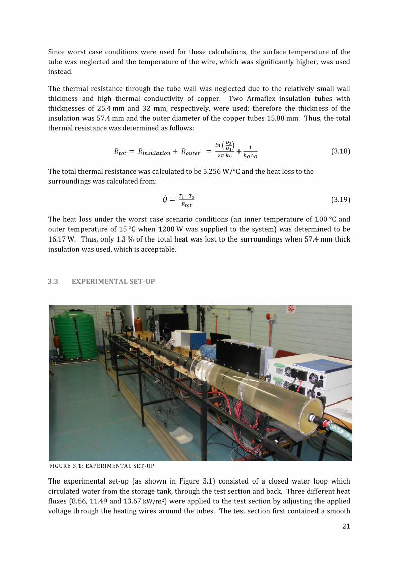
3.3 Experimental Set-up ...................................................................................................................................... 21
3.3.1 Tube Diameters .............................................................................................................................................. 23
3.3.2 Surface Roughness ........................................................................................................................................ 23
3.3.3 Calming Section .............................................................................................................................................. 28
3.3.4 Test Section ...................................................................................................................................................... 29
3.4 Data Reduction................................................................................................................................................. 31
3.4.1 Friction Factor ................................................................................................................................................ 31
3.4.2 Heat Transfer Coefficient ........................................................................................................................... 31

ii
3.4.3 Energy Balance ............................................................................................................................................... 32
3.5 Instruments ....................................................................................................................................................... 32
3.5.1 DC Power Supply ............................................................................................................................................. 32
3.5.2 Thermocouples ............................................................................................................................................... 32
3.5.3 Heating Wire .................................................................................................................................................... 33
3.5.4 Pressure Transducers .................................................................................................................................. 33
3.5.5 Flow meters ..................................................................................................................................................... 34
3.6 Experimental Procedure .............................................................................................................................. 34
3.7 Validation ........................................................................................................................................................... 35
3.7.1 Adiabatic Friction Factors .......................................................................................................................... 35
3.7.2 Diabatic Friction Factors ............................................................................................................................ 38
3.7.3 Heat Transfer Coefficients ......................................................................................................................... 39
3.8 Conclusion ......................................................................................................................................................... 40
4. Results ............................................................................................................................................................................ 42
4.1 Introduction ...................................................................................................................................................... 42
4.2 Smooth Tube ..................................................................................................................................................... 42
4.2.1 Friction Factors .............................................................................................................................................. 42
4.2.2 Heat Transfer ................................................................................................................................................... 44
4.3 Roughened Tube ............................................................................................................................................. 47
4.3.1 Friction Factors .............................................................................................................................................. 47
4.3.2 Heat Transfer Coefficients ......................................................................................................................... 49
4.4 Conclusion ......................................................................................................................................................... 51
5. Conclusion and Recommendations .................................................................................................................... 53
6. References .................................................................................................................................................................... 55
Appendix A: Surface Roughness .............................................................................................................................. A1
A.1 Sand Paper ........................................................................................................................................................ A2
A.2 Steel Brush ........................................................................................................................................................ A3
A.3 Hammering Process ...................................................................................................................................... A5
A.4 Sand Grading Analysis ................................................................................................................................. A7
Appendix B: Calibration .............................................................................................................................................. B1
B.1 Thermocouple Calibration ......................................................................................................................... B2
B.2 Pressure Transducer Calibration ............................................................................................................ B7
Appendix C: Matlab Codes .......................................................................................................................................... C1
C.1 Thermocouple Calibration .......................................................................................................................... C2
C.2 Adiabatic Tests ................................................................................................................................................. C3
C.3 Diabatic Tests ................................................................................................................................................... C6
C.4 Data Comparison ............................................................................................................................................. C9
C.5 Secondary Flow ............................................................................................................................................ C10
Appendix D: Protocol and Progress Reports ...................................................................................................... D1
D.1 Protocol .............................................................................................................................................................. D2
D.2 First Progress Report ................................................................................................................................... D6
D.3 Second Progress Report ............................................................................................................................... 42

iii
LIST OF TABLES
Table 2.1: Transition Reynolds Numbers for Different Heat Fluxes ........................................................... 7
Table 3.1: Temperature Differences at Different Heat Fluxes .................................................................... 19
LIST OF FIGURES
Figure 2.1: Different Inlet Geometries ..................................................................................................................... 5 Figure 2.2: Secondary Flow .......................................................................................................................................... 6 Figure 3.1: Experimental Set-up .............................................................................................................................. 21 Figure 3.2: Positive Displacement Pump and Accumulator ......................................................................... 22 Figure 3.3: Experimental Set-up .............................................................................................................................. 23 Figure 3.4: Moody Chart (Toprak, 2006) ............................................................................................................. 24 Figure 3.5: Steel Brush ................................................................................................................................................ 24 Figure 3.6: Steel Wire Mesh....................................................................................................................................... 25 Figure 3.7: Steel Rod..................................................................................................................................................... 25 Figure 3.8: Measuring Hammered Section .......................................................................................................... 25 Figure 3.9: Frictions Factor Comparison for Smooth and Roughened Tubes ...................................... 26 Figure 3.10: Pressure Comparison for Smooth and Roughened Tubes .................................................. 27 Figure 3.11: Thermal Resistance Experiment ................................................................................................... 27 Figure 3.12: Sand Roughened Tube ....................................................................................................................... 28 Figure 3.13: Calming Section .................................................................................................................................... 28 Figure 3.15: Schematic of Test Section ................................................................................................................. 29 Figure 3.14: Square-edged Inlet .............................................................................................................................. 29 Figure 3.16: Thermocouples Attached to Tube ................................................................................................. 30 Figure 3.17: Pressure Tap .......................................................................................................................................... 30 Figure 3.18: Mixer ......................................................................................................................................................... 30 Figure 3.19: Power Supply ......................................................................................................................................... 32 Figure 3.20: Heating Wire .......................................................................................................................................... 33 Figure 3.21: Differential Pressure Transducer .................................................................................................. 34 Figure 3.22: Coriolis Flow Meters ........................................................................................................................... 34 Figure 3.23: Validation of Adiabatic Friction Factor Results Inside the Smooth Tube ..................... 37 Figure 3.24: Validation of Adiabatic Friction Factor Results Inside the Roughened Tube ............. 38 Figure 3.25: Validation of Diabatic Friction Factor Inside the Smooth Tube ....................................... 39 Figure 3.26: Validation of Heat Transfer Data for the Smooth Tube........................................................ 40 Figure 4.1: Local Heat Transfer Coefficients for the Smooth Tube When 8.66 kw/m2 Heat Flux 43 Figure 4.2: Experimental Friction Factors for the Smooth Tube as a Function of Reynolds Number for Different Heat Fluxes .......................................................................................................................... 44 Figure 4.3: Experimental Heat Transfer Data for the Smooth Tube in terms of Nusselt Numbers against Reynolds Numbers for Different Heat Fluxes .................................................................................... 45 Figure 4.4: Local Heat Transfer Ratio for the Smooth Tube for Different Heat Fluxes .................... 46 Figure 4.5: Smooth Tube Heat Transfer Data in terms of the Colburn j-factors for Different Heat Fluxes .................................................................................................................................................................................. 47 Figure 4.6: Experimental Friction Factors for the Smooth Tube and Roughened Tubes as a Function of Reynolds Number for Different Heat Fluxes .............................................................................. 44 Figure 4.7: Experimental Heat Transfer Data for the Smooth Tube and Roughened Tubes in terms of Nusselt Numbers against Reynolds Numbers for Different Heat Fluxes ............................. 45 Figure 4.8: Local Heat Transfer Ratio for the Roughened Tube for Different Heat Fluxes ............. 50 Figure 4.9: Experimental Data for the Smooth Tube in terms of the Colburn j-factor ..................... 51

iv
NOMENCLATURE
A Area m2
D Diameter m
Cp Constant pressure specific heat J/kg K
EB Energy Balance
f Friction factor
Gr Grashof number
g Gravitational acceleration m/s2
h Convection heat transfer coefficient W/m2 °C
I Current A
j Colburn j-factor
k Thermal conductivity W/m K
K Minor losses
L Length m
Lc Characteristic linear dimension m
m Flow parameter
Mass flow rate kg/s
N Number of turns
Nu Nusselt number
ρr Resistivity Ω/m
Pr Prandtl number
Heat transfer rate W
Heat flux W/m2
R Resistance Ω
Re Reynolds number
St Stanton number
TS Temperature of surface °C
T∞ Temperature of fluid sufficiently far from surface °C
V Mean velocity of object relative to the fluid
Voltage
m/s
V
GREEK LETTERS
α Thermal diffusivity m2/s
β Coefficient of volume expansion
ε Heat transfer effectiveness
ρ Density of the fluid kg/m3
µ Dynamic fluid viscosity kg/ms
ѵ Kinematic Viscosity m2/s
Δh Head loss m
ΔP Pressure drop Pa
ΔT Temperature Difference °C

v
SUBSCRIPTS
avg Average
b Property evaluated at bulk temperature
conv Convection
i Inner
lam Laminar flow
o Outer
tot Total
trans Transitional flow
turb Turbulent flow
w Property evaluated at wall temperature
Wire property
cp Constant property solution (isothermal)
vp Variable property solution (non-isothermal)
1
1. INTRODUCTION
1.1 BACKGROUND
Flow in tubes has been extensively investigated since as early as 1883 especially focusing on
laminar and turbulent flow, while research has been done on the transitional flow regime since
the 1990’s. The transitional flow regime is where the Reynolds Number changes from laminar
to turbulent flow and it is usually avoided due to flow instabilities and uncertainties.
Transition occurs at a Reynolds number of 2 300 for uniform and steady flow in a horizontal
smooth tube with a rounded entrance (ASHRAE, 2009). However, this Reynolds number is
significantly affected when the inlet geometry and smoothness of the tube are changed, which
typically occur in heat exchangers in order to increase the heat transfer and efficiency. When
designing heat exchangers, the aim is to increase the heat transfer, while reducing the pressure
drop. Turbulent flow provides good heat transfer coefficients and high pressure drops, while
the opposite is true for laminar flow. Therefore, transitional flow will be able to provide higher
heat transfer coefficients compared to laminar flow, but also lower pressure drops compared to
turbulent flow. Although heat exchanger designers are usually advised to avoid flow in the
transitional flow regime (mainly due to the large fluctuations and uncertainties) it is not always
possible, due to design constraints. Thus, it is important to investigate flow through tubes with
different inlet geometries, inside surfaces as well as different boundary conditions.
Up to now, there are mainly two groups of people who have investigated flow in the transitional
flow regime. Professor A. J. Ghajar from Oklahoma State University as well as Professor J.P.
Meyer from the University of Pretoria, have both investigated flow through smooth tubes in the
transitional flow regime under diabatic conditions and adiabatic conditions. Meyer also
investigated the influence of enhanced tubes. Extensive work has been done in the Heat
Transfer Laboratory of the University of Pretoria on heat transfer in the transitional flow
regime, as well as on the influence of different inlet geometries and enhanced tubes on flow in
this flow regime. These studies proved that the transitional flow regime can be accurately
described and is not as chaotic and unpredictable as was believed earlier. However, since this
research was mainly focused on the influence of different inlet geometries and secondary flow
due to applied heat fluxes, the influence of a uniform surface roughness has not yet been
investigated.
1.2 PROBLEM STATEMENT
As indicated above, previous work has been done on flow in the transitional flow regime, but
these studies focused primarily on the influence of inlet geometries and secondary flow due to
the heat flux applied. The influence of surface roughness in the transitional flow regime has not
yet been investigated.
2
1.3 AIM
The purpose of this study was to investigate the influence of surface roughness at different heat
fluxes.
1.4 OBJECTIVES
The main objectives of this study will be:
To obtain the heat transfer and friction factor data for Reynolds numbers between 1 000
and 7 000 for water flowing through a smooth and roughened tube of the same
diameter.
To determine the boundaries of the transitional region for flow through a roughened
tube.
To investigate the influence of surface roughness in the transitional flow regime.
These objectives will be obtained by capturing the required information by means of an
experimental system.
1.5 SCOPE OF WORK
In chapter 2, a literature study is presented which was compiled on the basis of the work done
by Professor Meyer from the University of Pretoria and by Professor Ghajar from Oklahoma
State University, respectively, on flow in the transitional flow regime.
In chapter 3 details are given of the experimental set-up. An experimental set-up was designed
and built to measure the heat flux, mass flow rate, pressure and temperature of flow through a
smooth and roughened horizontal tube. Two copper tubes with an outer diameter of 15.88 mm
and a length of 1.8 m were used. The one tube was smooth on the inside, whereas the other
tube was roughened in order to obtain a relative roughness of 0.058. The Reynolds numbers
ranged between 1 000 and 7 000 for the smooth tube, and between 500 and 7 000 for the
roughened tube, in order to ensure that the entire transitional flow regime, as well as part of the
laminar and turbulent flow regimes, was covered. Three different heat fluxes (8.66, 11.14 and
13.92 kW/m2) were applied to the tubes by using T-type thermocouple wire. The Colburn j-
factors, and Nusselt numbers as a function of heat flux and Reynolds numbers were determined
from the experimental heat transfer data. The pressure drop measurements were used to
determine the adiabatic and diabatic friction factors. The data reduction and experimental
validation are also covered in this chapter
Chapter 4 contains the experimental results and Chapter 5 contains the conclusion as well as
recommendations for further work.

3
2. LITERATURE STUDY
2.1 INTRODUCTION
The transitional flow regime is where the fluid motion changes from laminar to turbulent flow.
Little design information is currently available about the heat transfer and pressure drop in the
transitional flow regime. Heat exchanger designers are therefore advised to remain outside this
region, mainly due to the flow instability and uncertainty in this region.
Up to now, there have been mainly two groups of people who have investigated flow in the
transitional flow regime. Professor A. J. Ghajar from Oklahoma State University and Professor
J.P. Meyer from the University of Pretoria have both investigated smooth tubes in the
transitional flow regime under diabatic and adiabatic conditions, while Meyer has investigated
the influence of enhanced tubes as well. Their work will briefly be discussed in this chapter; a
few fundamental concepts are, however, first revised.
2.2 REYNOLDS AND GRASHOF NUMBERS
Reynolds showed, as early as 1883, that the critical value at which transition occurs, is
dependent on the surrounding disturbances. Thus, for tubes, this value is a function of the tube
diameter, fluid velocity and viscosity. This is also known as the Reynolds number, which is a
dimensionless number of the ratio of the inertial forces to viscous forces. It also characterizes
flow regimes, for example, laminar flow in a tube occurs at lower Reynolds numbers, usually
below 2 300, while turbulent flow occurs at Reynolds numbers larger than 4 000. The
transitional flow regime is where the fluid motion changes from laminar to turbulent flow. For
a round pipe with water flowing through it, the Reynolds numbers in this region will be
between 2 300 and 10 000 (Cengel, 2006, p. 365).
For pipe-flow, the Reynolds number can be calculated using the following formula:
(2.1)
While the flow regime in forced convection is governed by the Reynolds number, the flow
regime in natural convection is governed by the Grashof number. This is a dimensionless
number which represents the ratio of the buoyancy force to the viscous force acting on a fluid.
Furthermore, it provides the main criterion to determine whether a fluid is laminar or turbulent
in natural convection (Cengel, 2006, pp. 509-510).
(2.2)

4
2.3 REYNOLDS ANALOGY
The Reynolds Analogy describes the relationship between pressure drop and heat transfer and
enables us to determine the friction, heat transfer or mass transfer coefficients when only one of
them is known. This analogy is restricted to cases where Pr = 1.
The equations can therefore be written as:
(2.3)
The Nusselt number is a dimensionless heat transfer coefficient and is named after William
Nusselt. It describes the enhancement of heat transfer in a fluid layer as a result of convection
relative to this layer. Hence, pure conduction heat transfer is represented by a Nusselt number
of 1 (Cengel, 2006). The Nusselt number is defined as:
(2.4)
The Prandtl number is a dimensionless parameter that describes the relative thickness of the
velocity and thermal boundary layers and is named after Ludwig Prandtl. The Stanton number
is also dimensionless parameters and can be described as follows (Cengel, 2006, pp. 365,812):
(2.5)
(2.6)
Due to the restrictions of the Reynolds Analogy, it has been modified to cover a range of Prandtl
numbers between 0.6 and 60. This new analogy, known as the Modified Reynolds Analogy or
Chilton-Colburn Analogy, can be expressed as:
P
1 (2.7)
h
P (2.8)
The Prandtl and Stanton numbers can also be used to determine the Colburn j-factor, which is
defined as follows:
(2.9)
Meyer and Olivier further modified the Reynolds Analogy to be valid for all flow regimes,
although it is restricted to water flowing through a smooth tube (Meyer & Olivier, 2010, p. 493).
It can be expressed as:
P P (2.10)

5
2.4 DIFFERENT INLET GEOMETRIES
The heat transfer coefficient along the tube and thus the transition from laminar to turbulent
flow is affected by the type of inlet geometry. There are typically four different types of inlets
that are used in the experiments and are shown in Figure 2.1.
1. Square-edged
This type of inlet is characterized by a sudden contraction of flow and simulates the
header of a shell-and-tube heat exchanger.
2. Re-entrant
This entrant contains a square-edged inlet with a tube inside and simulates a floating
header in a shell-and-tube heat exchanger.
3. Bellmouth
This inlet contains a smooth and gradual contraction and aims to reduce fouling,
although it is not commonly used in heat exchangers.
4. Hydro-dynamically fully-developed inlet
The diameter of this inlet section is the same as the pipe diameter of the test section.
This inlet is used to obtain a fully-developed velocity profile, since the velocity profile of
the other three inlets is always developing.
FIGURE 2.1: DIFFERENT INLET GEOMETRIES
Flow direction
6
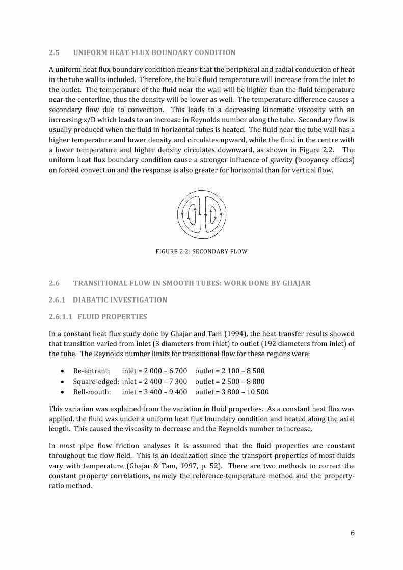
2.5 UNIFORM HEAT FLUX BOUNDARY CONDITION
A uniform heat flux boundary condition means that the peripheral and radial conduction of heat
in the tube wall is included. Therefore, the bulk fluid temperature will increase from the inlet to
the outlet. The temperature of the fluid near the wall will be higher than the fluid temperature
near the centerline, thus the density will be lower as well. The temperature difference causes a
secondary flow due to convection. This leads to a decreasing kinematic viscosity with an
increasing x/D which leads to an increase in Reynolds number along the tube. Secondary flow is
usually produced when the fluid in horizontal tubes is heated. The fluid near the tube wall has a
higher temperature and lower density and circulates upward, while the fluid in the centre with
a lower temperature and higher density circulates downward, as shown in Figure 2.2. The
uniform heat flux boundary condition cause a stronger influence of gravity (buoyancy effects)
on forced convection and the response is also greater for horizontal than for vertical flow.
FIGURE 2.2: SECONDARY FLOW
2.6 TRANSITIONAL FLOW IN SMOOTH TUBES: WORK DONE BY GHAJAR
2.6.1 DIABATIC INVESTIGATION
2.6.1.1 FLUID PROPERTIES
In a constant heat flux study done by Ghajar and Tam (1994), the heat transfer results showed
that transition varied from inlet (3 diameters from inlet) to outlet (192 diameters from inlet) of
the tube. The Reynolds number limits for transitional flow for these regions were:
Re-entrant: inlet = 2 000 – 6 700 outlet = 2 100 – 8 500
Square-edged: inlet = 2 400 – 7 300 outlet = 2 500 – 8 800
Bell-mouth: inlet = 3 400 – 9 400 outlet = 3 800 – 10 500
This variation was explained from the variation in fluid properties. As a constant heat flux was
applied, the fluid was under a uniform heat flux boundary condition and heated along the axial
length. This caused the viscosity to decrease and the Reynolds number to increase.
In most pipe flow friction analyses it is assumed that the fluid properties are constant
throughout the flow field. This is an idealization since the transport properties of most fluids
vary with temperature (Ghajar & Tam, 1997, p. 52). There are two methods to correct the
constant property correlations, namely the reference-temperature method and the property-
ratio method.

7
A characteristic temperature is chosen at which the non-dimensionalised properties (Cf , Re, Pr,
etc) are evaluated using the reference-temperature method. The constant property results at
that temperature can then be used to predict the variable-property behaviour.
The property-ratio method is often used in literature and the properties are evaluated at the
bulk temperature. The variable-property effects are then used as a function of the ratio of one
property evaluated at the bulk temperature to that temperature evaluated at the wall
temperature. The variation in viscosity is responsible for most property effects in liquids. Thus,
the property-ratio method for liquids is correlated by:
(2.11)
2.6.1.2 INFLUENCE OF INLET GEOMETRY ON PRESSURE DROP MEASUREMENTS, FRICTION FACTORS AND HEAT TRANSFER
Ghajar and Tam (1994, pp. 79-89) did a study to provide a heat transfer database across all flow
regimes in the entrance and fully developed regions for different inlet configurations. This data
base can be used to assist heat exchanger designers in predicting the heat transfer coefficient
along a circular horizontal tube. Ghajar further plotted graphs to show the effect of secondary
flow on the heat transfer coefficient. This illustrated that secondary flow will dominate after a
certain length-to-diameter ratio. The geometry of the inlet also influences the development of
the heat transfer coefficient along the pipe. The influence of the inlet geometry at the beginning
and end of transition was shown when the average heat transfer coefficients in terms of the
Colburn j-factor were plotted against the bulk Reynolds number. Based on these experimental
results, the limits for the Reynolds number range are
Re-entrant 2 000 < Re < 8 500
Square-edged 2 400 < Re < 8 800
Bell-mouth 3 800 < Re < 10 500
It is therefore clear that the heat transfer coefficient as well as the beginning and end of
transition, is influenced by the inlet geometry. Secondary flow increased along the pipe, which
caused the kinematic viscosity to decrease. Thus, the local bulk Reynolds number (beginning
and end of transition) also increased.
In another study, a uniform heat flux boundary condition is applied by attaching welding cables
to the copper plates at the pressure drop test section. Three different heat fluxes (3, 8 and
16 kW/m2) were used in this investigation and the results obtained were as follows (Ghajar &
Tam, 1997, pp. 52-64):
TABLE 2.1: TRANSITION REYNOLDS NUMBERS FOR DIFFERENT HEAT FLUXES
Heat flux [kW/m2] Re-entrant Square-edged Bell-mouth
0 2 870 < Re < 3 500 3 100 < Re < 3 700 5 100 < Re < 6 100
3 3 060 < Re < 3 890 3 500 < Re < 4 180 5 930 < Re < 8 730
8 3 350 < Re < 4 960 3 860 < Re < 5 200 6 480 < Re < 9 110
16 4 090 < Re < 5 940 4 450 < Re < 6 430 7 320 < Re < 9 560
8
The results prove that heating has a significant influence on the transition region. The increase
in the friction factor causes an increase in the lower and upper limits of the transition region,
compared to adiabatic flow (0 kW/m2). Ghajar also plotted the friction factor against Reynolds
number and the results showed that, while the influence of the heating was significant in the
laminar and transition regions, it had almost no effect on the friction factors in the turbulent
region. This is due to the secondary flow, since the velocity profile of the fluid changes due to
mixed convection, therefore the shear stress, fluid density as well as the friction factor, is also
changed. As the heat flux increases, the shear stress increases due to the change of velocity
profile and so the friction factor also increases. It can also be seen that the Reynolds numbers at
the beginning and end of the transition region increase with an increase in the heat flux applied.
The heating therefore delays the flow transition, or stabilizes the flow, thus causing it to go into
transition at higher Reynolds numbers.
The effect of the inlet geometry is identical when compared to the isothermal conditions. Early
transition occurred at the inlet that caused the most disturbances, while transition was delayed
at the inlet that caused the least disturbance.
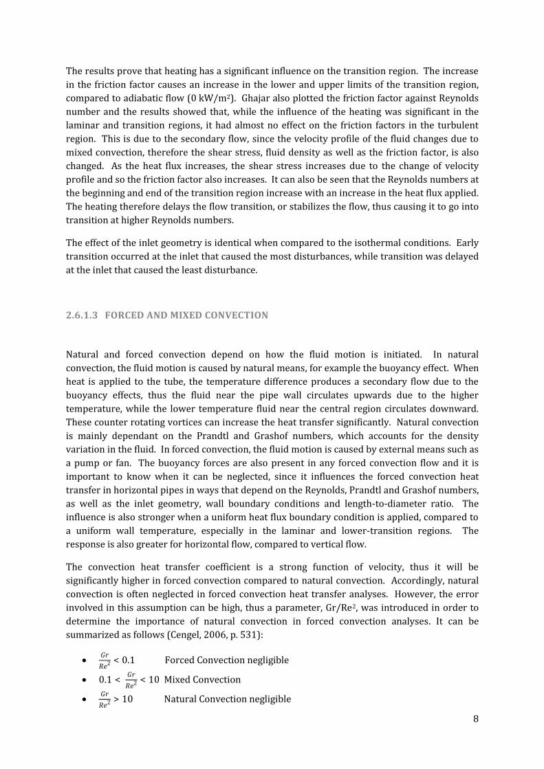
2.6.1.3 FORCED AND MIXED CONVECTION
Natural and forced convection depend on how the fluid motion is initiated. In natural
convection, the fluid motion is caused by natural means, for example the buoyancy effect. When
heat is applied to the tube, the temperature difference produces a secondary flow due to the
buoyancy effects, thus the fluid near the pipe wall circulates upwards due to the higher
temperature, while the lower temperature fluid near the central region circulates downward.
These counter rotating vortices can increase the heat transfer significantly. Natural convection
is mainly dependant on the Prandtl and Grashof numbers, which accounts for the density
variation in the fluid. In forced convection, the fluid motion is caused by external means such as
a pump or fan. The buoyancy forces are also present in any forced convection flow and it is
important to know when it can be neglected, since it influences the forced convection heat
transfer in horizontal pipes in ways that depend on the Reynolds, Prandtl and Grashof numbers,
as well as the inlet geometry, wall boundary conditions and length-to-diameter ratio. The
influence is also stronger when a uniform heat flux boundary condition is applied, compared to
a uniform wall temperature, especially in the laminar and lower-transition regions. The
response is also greater for horizontal flow, compared to vertical flow.
The convection heat transfer coefficient is a strong function of velocity, thus it will be
significantly higher in forced convection compared to natural convection. Accordingly, natural
convection is often neglected in forced convection heat transfer analyses. However, the error
involved in this assumption can be high, thus a parameter, Gr/Re2, was introduced in order to
determine the importance of natural convection in forced convection analyses. It can be
summarized as follows (Cengel, 2006, p. 531):
0 1 Forced Convection negligible
0 1
10 Mixed Convection
10 Natural Convection negligible

9
Mixed convection is when both natural and forced convection are significant in the heat transfer
analysis. It is not only dependant on the Reynolds and Prandtl numbers, but also on the Grashof
number in order to account for the density variation of the test fluid. The presence of natural
convection along with forced convection leads to higher Nusselt numbers in laminar flow.
The local heat transfer data obtained from the experiments can also be used to determine the
boundary between forced and mixed convection (Ghajar & Tam, 1994, pp. 83-84). For forced
convection, the ratio of the local peripheral heat transfer coefficient at the top and bottom of the
tube is close to unity (0.8 – 1.0), while it is much less than unity for natural convection.
The inlet geometry has a significant influence on the boundary between forced and mixed
convection. Based on the experimental results, the transition region limits for the re-entrant
and square-edged inlets are:
Re-entrant 2 157 < Re < 8 475
Square-edged 2 514 < Re < 8 791
These transition region limits are dependent on x/D since the physical properties of the fluid
vary with temperature. Forced convection dominated at higher Reynolds numbers and the heat
transfer ratio varied between 0.9 and 1, while mixed convection dominated at lower Reynolds
numbers. For mixed convection, the heat transfer coefficient ratio decreased with an increase in
the length-to-diameter ratio, and beyond 125 diameters from the tube entrance, the free
convection activity increased, while forced convection was less dominant. The increase in the
transition limits is solely due to the variation in the physical properties of the pipe. Due to the
increase of the fluid bulk temperature along the pipe, the kinematic viscosity of the fluid
decreases and this, in turn, causes an increase in the local bulk Reynolds numbers (Ghajar &
Tam, 1995, pp. 287-297).
Mixed convection dominates in the laminar and lower transition flow regions, while natural
convection can be assumed to be negligible in turbulent flow. The inlet configuration will
therefore have a minor influence on the heat transfer coefficient.
2.6.2 ADIABATIC INVESTIGATION
The following limits for the transition range were obtained from experiments done by Ghajar
and Madon on the pressure drop measurements of laminar-transition-turbulent flow (Ghajar &
Madon, 1992, p. 132):
Re-entrant 1 980 < Re < 2 600
Square-edged 2 070 < Re < 2 840
Bell-mouth 2 125 < Re < 3 200
The experimental set-up used for this study was designed in such a way that the flow in the test
section was fully developed. Thus, the measurements in the entrance region of transitional flow
were not considered. The fully developed skin friction coefficient was determined from the
measured pressure drop readings. (The skin friction coefficient corresponds to a friction
coefficient that accounts for pressure drop arising from shear stresses at the wall only.) The

10
data obtained indicated the influence of the inlet configuration at the start and end of transition.
Once again, the inlet that caused the most disturbances showed an early transition.
Isothermal flow conditions were also investigated by Ghajar and Tam, by ensuring that the inlet
and outlet bulk temperatures were equal within 0.4 °C (Ghajar & Tam, 1997). The Reynolds
number ranges for these conditions are:
Re-entrant 2 870 < Re < 3 500
Square-edged 3 110 < Re < 3 700
Bell-mouth 5 100 < Re < 6 100
The Reynolds number for the start of transition is taken as the first sudden change in the
friction factor. The Reynolds number for the end of transition corresponds to the Reynolds
number of the friction factor that first reaches the fully developed turbulent friction factor line.
The bulk Reynolds number for this study is significantly larger compared to the previously
mentioned study. This may be due to the properties of the test fluid, since different ethylene-
glycol-water mixtures were used. However, it can still be concluded that the transition
Reynolds number range can be manipulated by using different inlet geometries. By comparing
these Reynolds number ranges with the diabatic results obtained from Ghajar when a constant
heat flux was applied, it follows that the secondary flow, due to the applied heat, increases the
Reynolds number ranges. The Reynolds number ranges for the transition region was higher
during diabatic investigations than during adiabatic investigations, thus transition is delayed
when heat flux is applied.
2.7 TRANSITIONAL FLOW IN SMOOTH TUBES: WORK DONE BY MEYER
While Ghajar used different ethylene-glycol-water mixtures as the test fluid for all his
experiments, water was used as the test fluid in the experiments done by Meyer. A constant
wall temperature boundary condition was also used for the heat transfer experiments, while
Ghajar mainly used a constant heat flux boundary condition.
2.7.1 DIABATIC INVESTIGATION
Since the viscosity difference between the fluid at the wall and the bulk fluid, as well as the
effect of secondary flow, influences the friction factors, it is important to investigate the diabatic
friction factors. The results obtained from a heat transfer study done with water as the test
fluid, showed that transition is independent of the type of inlet that was used. Transition for all
inlet geometries was between Reynolds numbers of 2 100 and 3 000. These results were then
confirmed by pressure drop data that was measured independently from the heat transfer data
(Meyer & Olivier, 2011). This inlet-independency is due to the buoyancy effect, since the
buoyancy-induced secondary flows suppress the growth of the hydrodynamic boundary layer to
such a degree that the flow is fully developed. Thus, transition occurs at the fully developed
inl t’s t ansition oint and the effects of the inlet geometries are dampened by the secondary
flow. The secondary flow effects dominate the boundary-layer in such a way that the inlet
geometry effects are negligible.

11
This, however, is not applicable to all fluids and might be limited to water and other low Prandtl
number fluids. The results obtained from the studies done by Ghajar showed that transition
was inlet-dependant under diabatic conditions. Ghajar used water-glycol mixtures with heat
transfer for these studies which caused the different conclusions.
The data further showed an overall increase in the friction factors, compared to their adiabatic
experimental results. This is mainly due to the effects of secondary flow. The friction factor is
proportional to the wall shear stress, which is proportional to the velocity gradient at the wall.
The secondary flow distorts the velocity profile in such a way that the gradient at the wall is
much steeper, resulting in higher friction factors.
The following correlations were developed from the experimental data obtained by Olivier and
are valid for all inlet geometries:
Friction Factors
(2.12)
By expanding the Stanton number using equation 2.6, the following correlation for the
friction factor is obtained:
1
(2.13)
This correlation accurately predicted the friction factors for all the flow regimes within
1%. Although it is valid for all flow regimes, it is restricted to water in smooth tubes
only, because the results differ for high Prandtl number fluids.
Laminar heat transfer
0 1
(2.14)
This correlation predicted the heat transfer data accurately within 7 % and is valid for
developing and fully developed flow. Although the form is similar to those developed by
previous authors, the GrPr-term contains a negative power in the Prandtl number since
fluids with high Prandtl numbers have a higher viscosity and tend to resist secondary
flow motion.
Comment: 940 < Re < 2 522
4.43 < Pr < 5.72
1.5 x 10⁵ < Gr < 4.3 x 10⁵
0.695 <
< 0.85
289 <
< 373
12
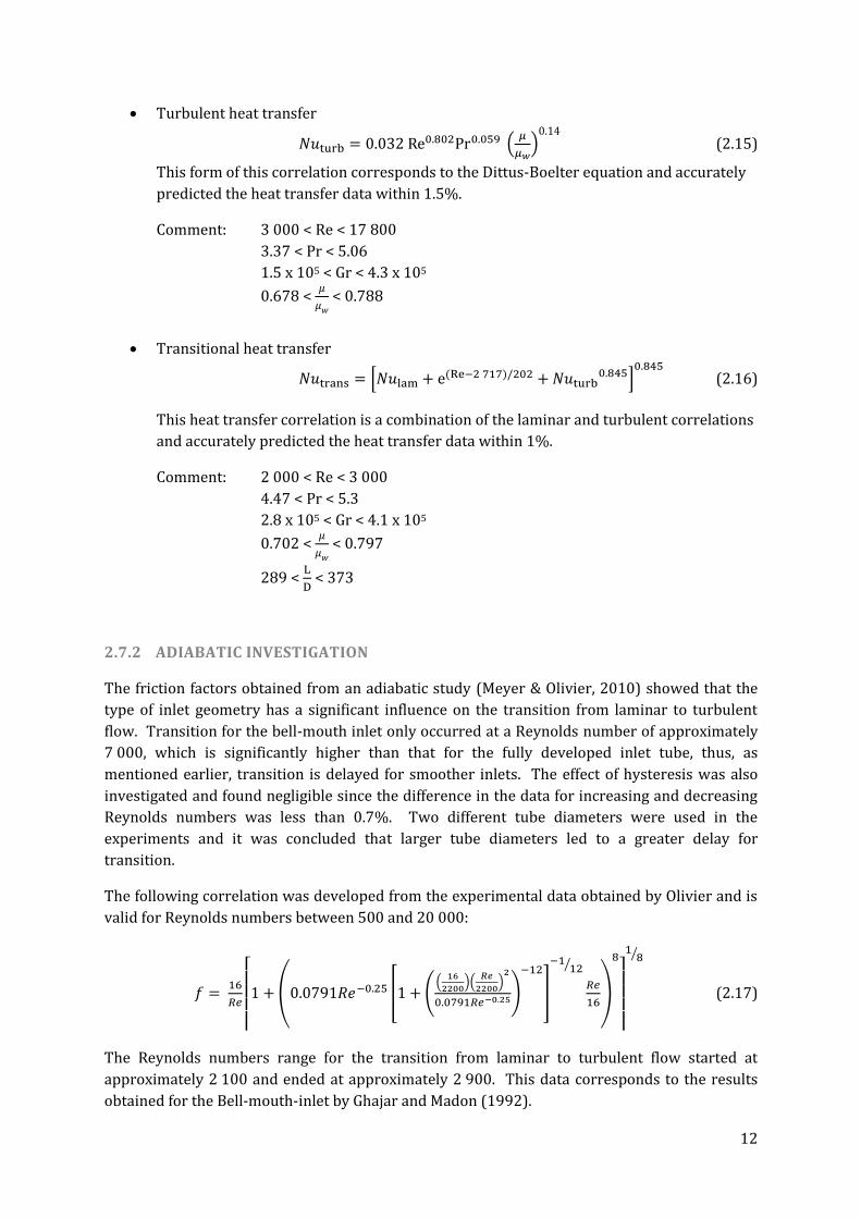
Turbulent heat transfer
0 1
(2.15)
This form of this correlation corresponds to the Dittus-Boelter equation and accurately
predicted the heat transfer data within 1.5%.
Comment: 3 000 < Re < 17 800
3.37 < Pr < 5.06
1.5 x 10⁵ < Gr < 4.3 x 10⁵
0.678 <
< 0.788
Transitional heat transfer
(2.16)
This heat transfer correlation is a combination of the laminar and turbulent correlations
and accurately predicted the heat transfer data within 1%.
Comment: 2 000 < Re < 3 000
4.47 < Pr < 5.3
2.8 x 10⁵ < Gr < 4.1 x 10⁵
0.702 <
< 0.797
289 <
< 373
2.7.2 ADIABATIC INVESTIGATION
The friction factors obtained from an adiabatic study (Meyer & Olivier, 2010) showed that the
type of inlet geometry has a significant influence on the transition from laminar to turbulent
flow. Transition for the bell-mouth inlet only occurred at a Reynolds number of approximately
7 000, which is significantly higher than that for the fully developed inlet tube, thus, as
mentioned earlier, transition is delayed for smoother inlets. The effect of hysteresis was also
investigated and found negligible since the difference in the data for increasing and decreasing
Reynolds numbers was less than 0.7%. Two different tube diameters were used in the
experiments and it was concluded that larger tube diameters led to a greater delay for
transition.
The following correlation was developed from the experimental data obtained by Olivier and is
valid for Reynolds numbers between 500 and 20 000:
(2.17)
The Reynolds numbers range for the transition from laminar to turbulent flow started at
approximately 2 100 and ended at approximately 2 900. This data corresponds to the results
obtained for the Bell-mouth-inlet by Ghajar and Madon (1992).

13
2.8 TRANSITIONAL FLOW IN ENHANCED TUBES: WORK DONE BY MEYER
The efficiency of heat exchangers can be increased by increasing the heat transfer surface area.
This will also decrease the flow rate in the tubes which leads to lower compressor and pumping
power required. For this reason, more heat exchangers will start to operate in the transitional
regime.
Garcia et al. (2005) investigated the thermo hydraulic behaviour in laminar, transitional and
turbulent flow by investigating helical wire coils fitted inside a round tube. They found that at
very low Reynolds numbers in laminar flow, the wires behave similar to a smooth tube, and heat
transfer is not improved. At Reynolds numbers between 200 and 1 000, the heat transfer rate is
significantly increased since the perturbation caused by the wire hinders the establishment of
the recirculation caused by buoyancy forces, so that forced convection heat transfer occurs. At
Reynolds numbers between 1 000 and 1 300, the heat transfer is significantly increased as well,
but this time due to the fact that the wire inserts promoted transition from laminar to turbulent
flow. It was further found that the heat transfer rate can be increased by 200 % while
maintaining a constant pumping power in the transitional region. In the turbulent flow regime,
the heat transfer is increased up to four times and the pressure drop up to nine times compared
to smooth tubes.
The results obtained from previous research performed on transitional flow, and especially the
results of Nunner and Koch, were analysed by Obot (Obot, et al., 1990). Nunner inserted
different types of circular rings along the length of the tube and investigated the heat transfer.
It was found that the roughness height was the main contributing factor that influenced
transition.
Meyer (2011, p. 55) investigated the friction factors and Nusselt numbers for enhanced tubes.
The outer walls of the enhanced tubes had a diameter of 15.8 mm and the inner-walls 14.6 mm.
The tubes had fins with a height of 0.395 mm and a fin apex angle of 27° inside. One tube had 25
fins with a helix angle of 18°, while the other tube had 35 fins with a helix angle of 27°.
2.8.1 DIABATIC INVESTIGATION
2.8.1.1 HEAT TRANSFER
The heat transfer coefficients for the enhanced tubes were calculated using the nominal surface
area which is based on the nominal diameter. Therefore their performance can easily be
compared with the results of the smooth tubes.
An interesting conclusion drawn from the diabatic heat transfer results is that transition for all
the tubes and flow types for fully developed and developing flow appeared at approximately the
same Reynolds numbers. Thus, for smooth tubes, transition is independent of the inlet
geometry and this was confirmed with the diabatic friction factor results. This was due to the
buoyancy-induced secondary flow inside the tubes, since water, which has a low Prandtl
number was used as the test fluid. These flow patterns usually occur in the transitional region
of low Prandtl number fluids. It also appeared that the roughness has little or no effect on the
transition region during heat transfer.

14
The heat transfer results further showed that the fins contribute negatively to the heat transfer
process in the laminar regime since they act as a barrier for secondary flow, thus preventing the
bulk fluid and the fluid at the tube wall from mixing with one another. The flow between the
fins is cooler than in the rest of the tube, therefore their viscosity is higher and this leads to a
higher shear stress. As a result, the fins have almost no effect on the spinning of the fluid at low
velocities.
The turbulent results, however, showed a significant increase in the heat transfer, although the
inlet geometry still had no influence on the turbulent regime. Between Reynolds numbers of
3 000 and 8 000, the results differ from those of the smooth tubes, since the j-factors increase
with Reynolds number. This is due to the fins that break the laminar viscous sub-layer, which
accounts for up to 60 % of the fluid’s temperature drop during turbulent flow. The helix angle
of the fins caused a further increase, since fins with a greater helix angle spin the fluid more
effectively.
A performance evaluation for these enhanced tubes was also performed and it was found that
the enhanced tubes became viable when the smooth tube Reynolds numbers exceeded 6 000
and peaked at Reynolds numbers of approximately 10 000. Thus, there was no performance
enhancement in the transition region.
2.8.1.2 FRICTION FACTORS
The friction factor and heat transfer data showed similar trends, with the result that higher
friction factors were obtained when compared to the data of smooth tubes.
In the laminar and turbulent regions, the friction factors were higher compared to the smooth
tubes. This is due to the fins that enhance the amount of mixing by spinning the fluid. A
secondary transition was observed in the turbulent results between Reynolds numbers of 3 000
and 10 000. The secondary transition was developed when the velocity of the fluid was high
enough for the helical fins to effectively spin it. The intensity of the spinning increased with an
increase in velocity, but stopped at a Reynolds number of approximately 10 000, from where
the friction factor started to decrease. The friction factors of this secondary transition region, as
well as the fully turbulent region were dependant on the helix angle, thus higher friction factors
were obtained for greater helix angles.
The friction factors in the transition region are independent of the Reynolds numbers and the
transition occurred between the same Reynolds numbers of 2 000 and 3 000, similar to those of
the smooth tubes. The critical Reynolds numbers were also found to be independent of the tube
or inlet geometry. This was also found in the heat transfer results, thus it can be concluded that
the results are independent of the measuring techniques.
2.8.2 ADIABATIC INVESTIGATION
There are three main conclusions that can be drawn from a comparison between the
experimental results of the smooth and enhanced tubes, namely:
15
1. There was an upward shift in the friction factors of the enhanced tubes.
This is due to the increase in surface roughness which increases the resistance to flow.
2. Transition occurred earlier compared to smooth tubes.
This is caused by the increased surface roughness.
3. There is a smooth second increase in the friction factors at Reynolds numbers between
3 000 and 10 000, which appears to be a secondary transition.
From the experimental results it follows that the effectiveness of the fins increases with
an increase in Reynolds numbers, thus with an increasing velocity. This secondary
transition may be caused by the effective rotation the fins bring about the fluid, since the
secondary transition did not occur in the results of studies using ring insert or dimpled
tubes.
The results showed that the fins were ineffective at lower Reynolds numbers and that they
become effective at rotating the fluid only as the velocity is increased. It was also concluded
that the developing boundary layer leads to an increase in the friction factors for fully
developed flow. In contrast, for developing flow, the tube roughness has a greater influence
than the effect of the boundary layer on the wall shear stress. The end of transition appeared to
be affected by the helix angle, since transition for the 27° helix angle occurred earlier than the
18° helix angle. It can subsequently be concluded that the roughness and angle of the fins has
an influence on the stability of the boundary layer.
When Meyer further compared a 19.1 mm tube with a 15.8 mm tube, the fully developed flow
results showed that transition was only influenced by the roughness height. Three 15.8 mm
enhanced tubes with a fin-height-to-diameter ratio of 0.027 showed that transition occurred at
a Reynolds number of approximately 1 870. The fourth tube had a diameter of 19.1 mm and the
fin-height-to-diameter ratio of 0.022 showed that transition only occurred at a Reynolds
number of 2 070. Since the same inlet geometry was used, it can be concluded that the only
geometrical aspect that influences transition is the fin-height-to-diameter ratio.
The laminar and turbulent friction factors were significantly higher than those of the smooth
tubes, but were also independent of the inlet geometry. The second transitional region which
occurred at Reynolds numbers between 3 000 and 10 000 was very stable and predictable,
compared to the first transitional region (Meyer & Olivier, 2010, p. 7).
2.9 SURFACE ROUGHNESS
Up to now, there have been no studies done on the influence of surface roughness in tubes on
heat transfer in the transitional flow regime. Smooth tubes were mostly considered, except for
Meyer and Olivier who investigated enhanced tubes as well. Dimpled tubes and tubes with
spiral inserts along the length of the tube have been investigated by Garcia et al., but no studies
have yet been done on tubes with a uniform surface roughness. The influence of surface
roughness in the transitional regime will therefore be investigated in this research report.

16
2.10 CONCLUSION
It is evident from the above results of the experiments done by Ghajar, Meyer and co-workers
that the geometry of the inlet influences the establishment of secondary flow, the beginning and
end of the heat transition region, as well as the development of the heat transfer coefficient
along the pipe. This effect however, is negligible when the test fluid is water or low Prandtl
number fluids, as was found in the studies done by Meyer.
The transition Reynolds number range is also influenced when heat flux is applied. The laminar
and transitional friction factors were increased by heating and this caused an increase of the
bulk Reynolds number, compared to the isothermal conditions. Heating delays the flow
transition or stabilizes the flow, thus causing it to go into transition at higher Reynolds
numbers.
Enhanced tubes were also investigated by Meyer and it was found that transition is independent
of the inlet geometry under diabatic and adiabatic conditions. The adiabatic heat transfer and
friction factors in the turbulent flow regime were higher compared to the smooth tubes. In
contrast, the laminar heat transfer coefficients were lower due to the fins that obstruct the
secondary flow and increase the mixing of the fluid. The helix angle had a negligible effect in the
laminar and transition regions and it is concluded that the fin-height-to-diameter ratio is the
only geometrical aspect that influences transition. However, a secondary transition occurred
between Reynolds numbers of 3 000 and 10 000 and was characterized by an increasing friction
factor with the Reynolds number. This is due to the fins that rotate the fluid, thus, the friction
factors increased with an increase in helix angle. The diabatic friction factors followed a trend
similar to that of the adiabatic friction factors.
The influence of surface roughness in the transitional flow regime will be further investigated as
no previous research has been done on tubes with a uniform surface roughness.
17
3. EXPERIMENTAL SET-UP
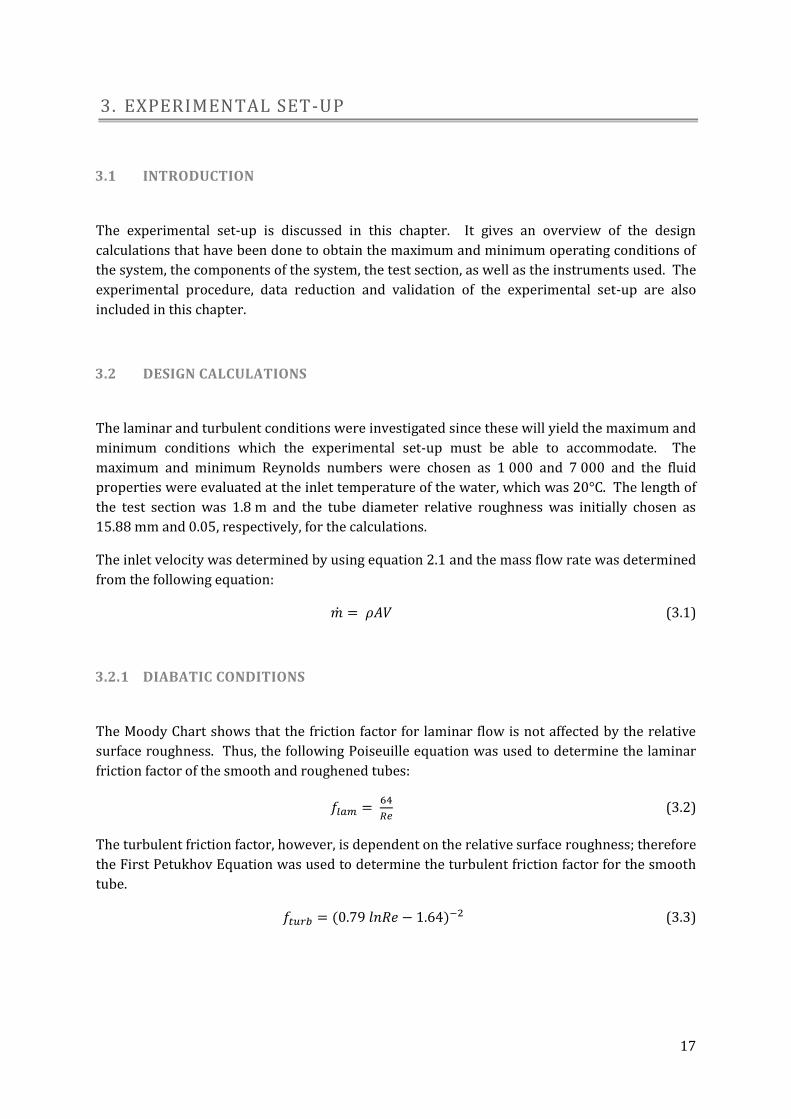
3.1 INTRODUCTION
The experimental set-up is discussed in this chapter. It gives an overview of the design
calculations that have been done to obtain the maximum and minimum operating conditions of
the system, the components of the system, the test section, as well as the instruments used. The
experimental procedure, data reduction and validation of the experimental set-up are also
included in this chapter.
3.2 DESIGN CALCULATIONS
The laminar and turbulent conditions were investigated since these will yield the maximum and
minimum conditions which the experimental set-up must be able to accommodate. The
maximum and minimum Reynolds numbers were chosen as 1 000 and 7 000 and the fluid
properties were evaluated at the inlet temperature of the water, which was 20°C. The length of
the test section was 1.8 m and the tube diameter relative roughness was initially chosen as
15.88 mm and 0.05, respectively, for the calculations.
The inlet velocity was determined by using equation 2.1 and the mass flow rate was determined
from the following equation:
(3.1)
3.2.1 DIABATIC CONDITIONS
The Moody Chart shows that the friction factor for laminar flow is not affected by the relative
surface roughness. Thus, the following Poiseuille equation was used to determine the laminar
friction factor of the smooth and roughened tubes:
(3.2)
The turbulent friction factor, however, is dependent on the relative surface roughness; therefore
the First Petukhov Equation was used to determine the turbulent friction factor for the smooth
tube.
(3.3)

18
The turbulent friction factor for the roughened tube was determined from the Modified
Colebrook equation:
(3.4)
The pressure drop for the smooth and rough tubes (both flow regimes) was calculated as
follows:
(3.5)
A constant heat flux has been applied to the tubes by means of T-thermocouples with the
following properties (Omega, 2012):
Resistivity: 50 µΩ/m
Thermal conductivity: 19.5 W/mK
Maximum operating temperature: 150 °C
Melting temperature 1225-1300 °C
Overall wire diameter: 0.001 m
Constantan diameter 0.00025 m
The power supply used for the experiments could supply a maximum power of 1.5 kW and
360V.
The number of turns of the thermocouple wire along the tube and the length of the
thermocouple wire were determined as follows:
(3.6)
(3.7)
In order to decrease the resistance of the wire, three thermocouple wires were placed in
parallel. Thus, each wire was a third of the initial length calculated above.
The resistance of the wire was determined using the following equation:
(3.8)
a all l
1 (3.9)
Since a maximum of 360 V could be supplied by the power source, the power supplied and the
current through the wire were then determined from:
(3.10)
(3.11)
The power and current were calculated as 1 275 W and 3.542 A. Finally the temperature
difference between the inlet and outlet was determined, using the flowing equation:

19
(3.12)
The temperature difference was calculated as 24.4 °C for laminar flow and 3.487 °C for
turbulent flow. Thus, the average temperature difference across the tubes was calculated to be
13.94 °C. These conditions were acceptable since the temperature difference was large enough
to obtain accurate measurements from the thermocouples. Temperature differences less than
1 °C are difficult to measure and could lead to inaccurate results.
The heat flux supplied to the copper tubes was obtained by dividing the heat applied by the
surface area as follows:
(3.13)
Since the experiments had to be conducted at different heat fluxes, three different heat fluxes
corresponding to three different power inputs which lead to reasonable temperature
differences were investigated using the above method. The results are tabulated in Table 3.1.
The maximum conditions appear in the first column, while the remaining three columns show
the results at the desired heat fluxes.
TABLE 3.1: TEMPERATURE DIFFERENCES AT DIFFERENT HEAT FLUXES
Q [W] 1275 1250 1000 750
q [kW/m
2]
14.20 13.92 11.14 8.35
Laminar Re = 1 000
Turbulent Re = 7 000
Laminar Re = 1 000
Turbulent Re = 7 000
Laminar Re = 1 000
Turbulent Re = 7 000
Laminar Re = 1 000
Turbulent Re = 7 000
V [V] 360 360 356.427 356.427 318.798 318.798 276.087 276.087
I [A] 3.542 3.542 3.507 3.507 3.137 3.137 2.717 2.717
24.4 3.478 23.92 3.418 19.134 2.735 14.351 2.051
13.94 13.67 10.93 8.201
3.2.2 MINOR PIPE LOSSES
In addition to the friction loss, there are also additional minor losses due to:
Pipe entrances or exits
Sudden expansion and contraction
Bends, elbows, tees and other fittings
Open or partially closed valves
Gradual expansions or contractions
The loss coefficients were obtained from tables and afterwards the system head loss was
computed using the following equation (White, 2009, p. 383):
(3.14)

20
The pressure losses in the pipes and fittings were determined by (Cengel, 2006, p. 465):
(3.15)
For laminar flow the head loss and pressure drop were calculated as 0.0181 m and 177.2 Pa,
respectively, in the smooth and roughened tubes. These values increased significantly in
turbulent flow to 0.55 m and 5.38 kPa in the smooth tube, and 1.02 m and 9.94 kPa in the
roughened tube.
3.2.3 OVERALL SYSTEM PRESSURE LOSS
The total pressure loss value of the experimental set-up was determined by adding the pressure
loss of the test section to the pressure loss due to the pipes and fittings. This value was
compared to the pump capacity in order to verify that the pump is sufficient. If the
requirements were not met, other parameters of the test section, for example the length or tube
diameter, had to be adjusted.
The maximum pressure loss for this experimental set-up was 10.7 kPa and occurred during
turbulent flow in the roughened tube. This was less than the maximum capacity of 500 kPa of
the SP3 Cemo pump that had been used.
3.2.4 INSULATION AND HEAT LOSS
Armaflex tubes with a thermal conductivity of 0.034 W/m2K were used as insulation for the
copper tubes in order to prevent heat loss to the surroundings. Turbulent flow conditions were
used for the calculations, since most heat transfer occurs during turbulent flow.
Free convection occurs on the outside of the insulation to the surroundings, thus the outer heat
transfer coefficient was between 2 and 25 W/m2K. The latter (25 W/m2K) was therefore used
for the remaining calculations. The inner heat transfer coefficient for turbulent flow was
obtained from the following Nusselt number relation:
(3.16)
The turbulent inner heat transfer coefficient is 2249 W/m2°C and, by using the exit water
temperature, the surface temperature can be determined from:
(3.17)
The surface temperature at the end of the tube was determined to be 30 °C. The surface
temperature of the tube increases linearly, thus the maximum temperature will be at the exit of
the tube. The temperature of the thermocouple wire also increased due to the current flowing
through it. For a current of approximately 1 A passing through each wire (thus a total of 3 A),
the temperature of the thermocouple wire was estimated to be 100 °C.
21
Since worst case conditions were used for these calculations, the surface temperature of the
tube was neglected and the temperature of the wire, which was significantly higher, was used
instead.
The thermal resistance through the tube wall was neglected due to the relatively small wall
thickness and high thermal conductivity of copper. Two Armaflex insulation tubes with
thicknesses of 25.4 mm and 32 mm, respectively, were used; therefore the thickness of the
insulation was 57.4 mm and the outer diameter of the copper tubes 15.88 mm. Thus, the total
thermal resistance was determined as follows:
(3.18)
The total thermal resistance was calculated to be 5.256 W/°C and the heat loss to the
surroundings was calculated from:
(3.19)
The heat loss under the worst case scenario conditions (an inner temperature of 100 °C and
outer temperature of 15 °C when 1200 W was supplied to the system) was determined to be
16.17 W. Thus, only 1.3 % of the total heat was lost to the surroundings when 57.4 mm thick
insulation was used, which is acceptable.
3.3 EXPERIMENTAL SET-UP
The experimental set-up (as shown in Figure 3.1) consisted of a closed water loop which
circulated water from the storage tank, through the test section and back. Three different heat
fluxes (8.66, 11.49 and 13.67 kW/m2) were applied to the test section by adjusting the applied
voltage through the heating wires around the tubes. The test section first contained a smooth
FIGURE 3.1: EXPERIMENTAL SET-UP

22
and then a roughened tube, both with an outer diameter of 15.88 mm and a length of 1.8 m, to
investigate the influence of surface roughness.
The test fluid was water and the temperature of the 1 000 litre reservoir was maintained at
20 °C. The water was circulated through the system via an electronically controlled positive
displacement pump with a maximum flow rate of 2 670 litre/h.
Flow pulsations were introduced into the system due to the positive displacement pumps. A
70 litre accumulator was installed before the flow meters and the test section in order to
decrease the pulsations. The accumulator was fitted with a rubber bladder filled with air to
dampen the fluctuations. This ensured a constant pressure at the inlet of the test section.
A bypass valve was inserted between the accumulator and the flow meters to allow the water to
flow back to the tank. The bypass valve was also used to increase the back pressure on the
pump, since the pulsations decreased with increasing pump speed. Therefore during
experiments, the supply valve was partially closed and the bypass valve partially open, so that
the speed of the pump had to be increased in order to supply the correct flow rate of water to
the test section, which resulted in reduced pulsations.
Two Coriolis flow meters with different capacities were installed in parallel to measure the
mass flow rate. Since the flow meters had different capacities, they were used according to the
flow rate requirements. After the flow meters, the fluid flowed through the calming section to
the experimental test section and then back into the reservoir.
The flow rates were controlled by the frequency drives that were connected to the positive
displacement pumps, therefore the required flow rate was obtained by increasing or decreasing
the pump speed. The frequency drives were also connected to a personal computer via the
data-acquisition system. A Labview program was used to record the data points and a Matlab
program was used to determine the Reynolds numbers, friction factors, Nusselt numbers, and
Colburn j-factors.
FIGURE 3.2: POSITIVE DISPLACEMENT PUMP AND ACCUMULATOR

23
The basic lay-out of the experimental set-up is shown in Figure 3.3.
FIGURE 3.3: EXPERIMENTAL SET-UP
3.3.1 TUBE DIAMETERS
Previous experiments conducted by Ghajar and Meyer used hard-drawn copper tubes with
outside diameters of 15.88 mm and 19.1 mm. For the present study, tubes with an outside
diameter of 15.88 mm have been used, since previous experiments were done with this
diameter and the new data can thus be compared with the existing data of Ghajar and Meyer. A
theoretical model of the experimental set-up verified that the pump capacity will accommodate
this diameter with the required length of the test section.
3.3.2 SURFACE ROUGHNESS
The aim of the experiment was to determine the influence of surface roughness in the
transitional flow regime. Thus the experimental results of a smooth and rough tube had to be
compared. The Moody Chart was used as a reference to determine whether the relative surface
roughness is sufficient, since the relative roughness lines corresponding to the roughened tube
should be well above the relative roughness line of a smooth tube between Reynolds numbers
of 1 000 and 7 000. From the Moody Chart it was concluded that a relative roughness of 0.001
would be sufficient.

24
FIGURE 3.4: MOODY CHART (TOPRAK, 2006)
Various attempts were made in order to roughen the tube and the results of the surface
roughness tests done by Metlab can be found in Appendix A. The first attempt was carried out
by fixing 40-grit sandpaper with double-sided tape to a 10 mm wooden dell. The dell was then
forced through the copper tube while turning it in order to obtain a uniform pattern. The
surface roughness was determined to be 1.67 µm which corresponded to a relative roughness of
0.00011. From the Moody Chart it was concluded to be insufficient.
A second approach was to use a steel brush. A 31 mm diameter steel brush was trimmed to
14.5 mm and fixed to a steel rod with wire. The rod was forced back and forth through the
copper tube while turning it with a vice grip. A surface roughness of 2.091 µm was obtained
which was twice as rough as the previous attempt, but still insufficient since it only
corresponded to a relative roughness of 0.00015. Figure 3.5 shows a new steel brush that has
been slightly trimmed, while the bottom brush has been used to roughen the tube.
A steel wire mesh was also rolled into a tube and then sewn together using one of the mesh
wires. The mesh was then placed inside the copper tube and the ends were folded over the tube
end to prevent the mesh from moving inside the tube. Although the mesh created a roughness
which would have been suitable, this concept was not used since it corresponds to heat transfer
enhancement instead of surface roughness. Using a left-hand and right-hand 14 mm tap was
also considered, but not used, since it once again corresponded to heat transfer enhancement
instead of surface roughness.
FIGURE 3.5: STEEL BRUSH

25
A process similar to knurling was used next. A 14 mm EN24 Steel rod was roughened on a lathe
by cutting various random grooves into the rod, until a pattern similar to the desired pattern on
the inside of the roughened tube was obtained. The steel rod was then fixed to a 2 m thinner
rod by cutting screw thread on the outside of the thin long rod and cutting a threaded hole
inside the roughened rod, as shown in Figure 3.7.
The total length of the roughened rod is 10 cm; therefore intervals of 8 cm were marked on the
copper tube. Two centimeters were allowed for a safety factor to ensure that the interval which
was hammered always had the roughened rod on the inside of the whole interval. Another thin
steel rod, with 8 cm intervals marked on it, as well, was inserted from the other side of the
copper tube and pressed against the roughened rod. This further ensured that the whole
hammered section always contained the roughened rod. A kinetic hammer was used to hammer
the copper tube while turning it slowly to ensure that the whole circumference is hammered.
After the entire 8 cm interval had been hammered, the roughened rod was pushed forward 8 cm
to hammer the next interval. Figure 3.8 further illustrates how the hammered interval was
monitored in order to prevent hammering a section that does not contain the rod.
Another piece of the same 15.88 mm copper tube that was used for the smooth and roughened
tubes was also roughened using the same method. This small tube was then analyzed to
determine the surface roughness. Metlab reported that the roughness of the tube could not be
measured since the needle got stuck in the grooves of the rough surface and that the tub ’s
surface profile falls outside the capabilities of their roughness tester. The maximum capability
FIGURE 3.7: STEEL ROD
FIGURE 3.8: MEASURING HAMMERED SECTION
FIGURE 3.6: STEEL WIRE MESH

26
of their equipment is a surface roughness of 16 µm and when dividing this with the inner tube
diameter of 14.46 mm, a relative roughness of 0.001 was obtained. This roughness was
regarded as sufficient since the corresponding friction factors on the Moody Chart varied
between 0.044 and 0.035 for Reynolds numbers between 3 000 and 7 000, which is acceptable.
Unfortunately, during the adiabatic tests on the roughened tube, it was found that the graphs of
the Friction Factor against Reynolds number (Figure 3.9) and Pressure against Reynolds
number (Figure 3.10) were almost identical to that of the smooth tube. Although there is a
slight increase in the friction factor in the transitional region, it is too small to make valid
conclusions on the influence of surface roughness. The increase in friction factor in the laminar
and turbulent regions, as well as the increase in pressure drop over the whole flow regime, is
negligible.
FIGURE 3.9: FRICTIONS FACTOR COMPARISON FOR SMOOTH AND ROUGHENED TUBES

27
FIGURE 3.10: PRESSURE COMPARISON FOR SMOOTH AND ROUGHENED TUBES
On of P andtl’s st d nts Nikuradse investigated the influence of relative roughness on the
friction factor in the turbulent flow regime by gluing sand grains of a known size onto the inner
surface of a tube (Cengel, 2006). Since these experiments were adiabatic, the thermal
conductivity of the glue and sand grains was of no importance. For this study, both the heat
transfer coefficient and friction factor were investigated, therefore the thermal conductivities of
the glue and sand grains should be as high as possible. Unfortunately high thermal conductivity
glues need to be imported and due to time constraints, cyanoacrylate (superglue) was used
since it bonds instantly when it comes into contact with two surfaces, but flows like water when
it is in contact with one surface only. Silica sand was used since the grains are relatively large
and of similar size.
The thermal resistance of the glue and silica sand was investigated with a small experiment
consisting of a smooth and a roughened tube and an isolated tube in between, as shown in
Figure 3.11. Both copper tubes had 3 thermocouples mounted on the top and sides. Water at
60 °C was pumped through the tubes and the temperatures were recorded in order to
determine whether there was any significant difference. Since there was no significant
difference between the measured temperatures of the two tubes, it was concluded that the
influence of the thermal resistance of the sand and the grains was negligible.
FIGURE 3.11: THERMAL RESISTANCE EXPERIMENT

28
A filter was also added after the test tubes in this experiment, as well as in the overall test section, to prevent loose sand grains from entering the system. After each test, the filter was checked and since it was clean, it was concluded that the cyanoacrylate and silica sand were able to withstand high temperatures and flow rates.
A Particle Size Distribution test using a Mastersizer 2000E was done in order to determine the
average grain size. The result analysis report can be found in Appendix A and since 90 % of the
sand grains in the sample had a diameter of 835.737 um, it was concluded that the average grain
size was 0.84 mm. This resulted in a relative roughness of 0.058, which was sufficient for the
tube to be considered as a rough tube.
3.3.3 CALMING SECTION
The set-up contained a calming section to remove any unsteadiness in the flow and ensure a
uniform velocity distribution before the fluid entered the test section. An existing calming
section shown in Figure 3.13, made by a previous final year student, Mr. Eric Mkhontho, was
modified and used (Mkhontho, 2011). It consisted of a 12 cm diameter Perspex tube with two
sieves on the inside. The original exit of the calming section was removed and a new Perspex
plate with a 15.88 mm fitting was glued to the calming section in order to connect the smooth
and roughened tube to it.
FIGURE 3.13: CALMING SECTION
FIGURE 3.12: SAND ROUGHENED TUBE

29
3.3.4 TEST SECTION
Square-edged inlets were used for both tubes. This type of inlet is characterized by a sudden
contraction from the calming section diameter to the test tube diameter. Therefore the copper
tubes were directly connected to the calming section with a compression fitting, as shown in
Figure 3.14. The test sections were manufactured from hard-drawn copper tubes with an inside
diameter of 14.46 mm, outside diameter of 15.88 mm and length of 1.8 m. Both tubes were
insulated with 54.7 mm thick Armaflex insulation with a thermal conductivity of 0.034 W/mK.
The heat loss was estimated to be 1.3 %.
A schematic lay-out of the test section is shown in Figure 3.15.
FIGURE 3.15: SCHEMATIC OF TEST SECTION
To obtain a constant heat flux boundary condition, T-type thermocouples with a Constantan
wire diameter of 0.25 mm, were wound around both copper tubes in the test section. Three
thermocouple wires were wound around the copper tubes in order to decrease the resistance
and current flowing through the wire, in comparison to using a single wire.
Thermocouples were also placed along the tubes to measure the temperature at the desired
locations. Four thermocouples were fixed 90° apart around the periphery of the tube. There
were 11 thermocouple stations spaced 170 mm from each other along the length of the tube and
therefore 44 thermocouples were used to measure the wall temperature on each tube. Another
thermocouple station at the mixing section consisted of two thermocouples at the top and
bottom of the tube. These thermocouples were soldered to the tube by first drilling a 1.5 mm
depression into the tube. Flux and solder were then inserted into the depression and heated
until melting point. The calibrated thermocouple was then inserted into the depression and the
FIGURE 3.14: SQUARE-EDGED INLET

30
heat was removed in order for the tube to cool down. The thermocouples were checked to
ensure good contact with the tube.
Two pressure taps were installed by silver soldering a 30 mm long capillary tube on each end of
the copper tubes. A 1.5 mm hole was then drilled through the capillary tube and the copper
tube. This small diameter was chosen to ensure that the taps did not cause flow obstruction in
the tubes and that the diameter is less than 10 % of th t st t b ’s inn diam t All th b s
were removed from the inside of the copper tube, since they could cause a local increase in
pressure which would have led to incorrect readings. A bush tap with a “q i k l as ” o ling
was inserted over the holes and soldered to the copper tubes, as shown in Figure 3.16. The
pressure taps were connected to the differential pressure transducer by using nylon tubing.
A mixer was inserted at the end of the test section. This mixed the water in the pipe to ensure a
uniform temperature in the pipe and the temperature measurements were then taken at the
end of the mixer tube. It was manufactured from a copper tube with an inside and outside
diameter of 20 mm and 22 mm, respectively. Six copper plate fins with a length if 30 mm were
soldered together, alternating between horizontal and vertical, as shown in Figure 3.18 The
mixers split the thermal layer in half, mixed it, and then split and mixed it again and again to
ensure a uniform temperature throughout the cross-section of the tube. Two thermocouples
were placed at the end of the mixer to measure the uniform exit temperature.
FIGURE 3.16: THERMOCOUPLES ATTACHED TO TUBE
FIGURE 3.17: PRESSURE TAP
FIGURE 3.18: MIXER

31
3.4 DATA REDUCTION
This section discusses the methodology used to obtain the heat transfer coefficients and friction
factors for smooth and roughened tubes.
3.4.1 FRICTION FACTOR
The friction factor for one-dimensional flow with a uniform density in smooth tubes of length L
and diameter D, can be written in terms of the overall pressure drop, by using equations 3.1 and
3.5:
(3.20)
was obtained from the differential pressure transducers and the fluid properties are
calculated at the bulk fluid temperature, which is the same as the mean temperature defined by
equation 3.22. This temperature was also used to determine the Reynolds, Nusselt, Prandtl and
other dimensionless groups.
3.4.2 HEAT TRANSFER COEFFICIENT
Heat transfer was achieved by supplying heat to the system by the thermocouples that were
wound around both tubes. The electric power delivered to the system was determined from the
voltage applied to the system and the known electrical resistance, using equation 3.10. The
resistance of the thermocouple wire was then determined using equations 3.8 and 3.9.
Three different heat fluxes were applied to the tubes. The local heat flux can be determined
from:
(3.21)
A constant heat flux is applied to the tubes, thus the temperature of the water flowing through it
will increase linearly. Therefore, the mean fluid temperature is the average of the inlet and
outlet temperature:
(3.22)
The surface temperature of the tube at the desired locations can be obtained from the
thermocouple readings. Since there are four thermocouples at each location, the average of the
four readings will be used. The heat transfer coefficient can then be determined from the
following equation since the heat flux, as well as the surface and mean water temperature at a
specific location, is known:
(3.23)
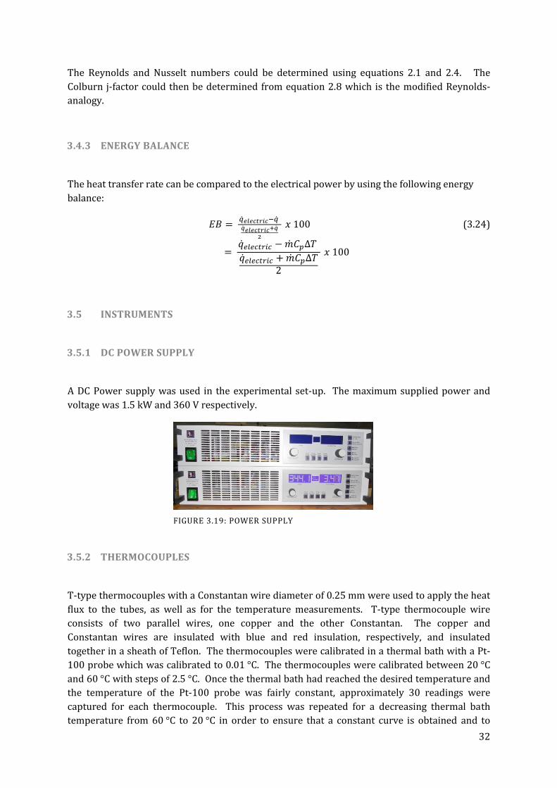
32
The Reynolds and Nusselt numbers could be determined using equations 2.1 and 2.4. The
Colburn j-factor could then be determined from equation 2.8 which is the modified Reynolds-
analogy.
3.4.3 ENERGY BALANCE
The heat transfer rate can be compared to the electrical power by using the following energy
balance:
(3.24)
3.5 INSTRUMENTS
3.5.1 DC POWER SUPPLY
A DC Power supply was used in the experimental set-up. The maximum supplied power and
voltage was 1.5 kW and 360 V respectively.
3.5.2 THERMOCOUPLES
T-type thermocouples with a Constantan wire diameter of 0.25 mm were used to apply the heat
flux to the tubes, as well as for the temperature measurements. T-type thermocouple wire
consists of two parallel wires, one copper and the other Constantan. The copper and
Constantan wires are insulated with blue and red insulation, respectively, and insulated
together in a sheath of Teflon. The thermocouples were calibrated in a thermal bath with a Pt-
100 probe which was calibrated to 0.01 °C. The thermocouples were calibrated between 20 °C
and 60 °C with steps of 2.5 °C. Once the thermal bath had reached the desired temperature and
the temperature of the Pt-100 probe was fairly constant, approximately 30 readings were
captured for each thermocouple. This process was repeated for a decreasing thermal bath
temperature from 60 °C to 20 °C in order to ensure that a constant curve is obtained and to
FIGURE 3.19: POWER SUPPLY
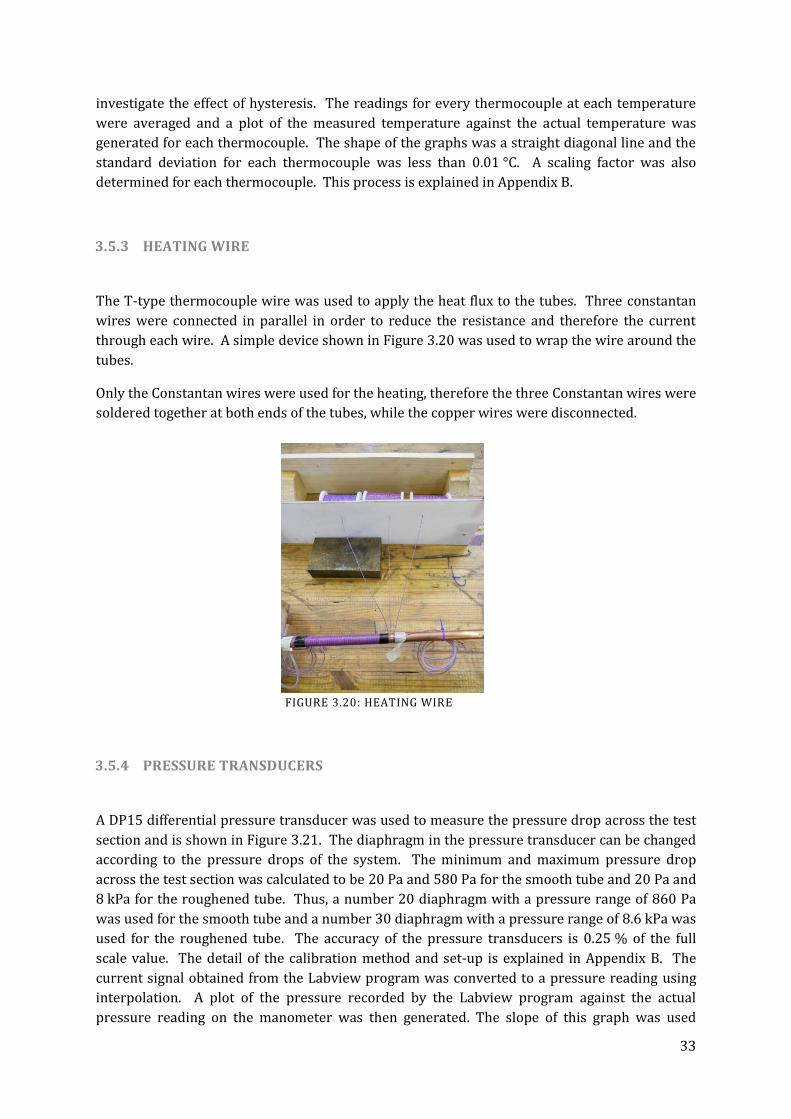
33
investigate the effect of hysteresis. The readings for every thermocouple at each temperature
were averaged and a plot of the measured temperature against the actual temperature was
generated for each thermocouple. The shape of the graphs was a straight diagonal line and the
standard deviation for each thermocouple was less than 0.01 °C. A scaling factor was also
determined for each thermocouple. This process is explained in Appendix B.
3.5.3 HEATING WIRE
The T-type thermocouple wire was used to apply the heat flux to the tubes. Three constantan
wires were connected in parallel in order to reduce the resistance and therefore the current
through each wire. A simple device shown in Figure 3.20 was used to wrap the wire around the
tubes.
Only the Constantan wires were used for the heating, therefore the three Constantan wires were
soldered together at both ends of the tubes, while the copper wires were disconnected.
3.5.4 PRESSURE TRANSDUCERS
A DP15 differential pressure transducer was used to measure the pressure drop across the test
section and is shown in Figure 3.21. The diaphragm in the pressure transducer can be changed
according to the pressure drops of the system. The minimum and maximum pressure drop
across the test section was calculated to be 20 Pa and 580 Pa for the smooth tube and 20 Pa and
8 kPa for the roughened tube. Thus, a number 20 diaphragm with a pressure range of 860 Pa
was used for the smooth tube and a number 30 diaphragm with a pressure range of 8.6 kPa was
used for the roughened tube. The accuracy of the pressure transducers is 0.25 % of the full
scale value. The detail of the calibration method and set-up is explained in Appendix B. The
current signal obtained from the Labview program was converted to a pressure reading using
interpolation. A plot of the pressure recorded by the Labview program against the actual
pressure reading on the manometer was then generated. The slope of this graph was used
FIGURE 3.20: HEATING WIRE

34
during each test to convert the pressure reading from current to Pascal. However, the off-set
differed for each test and ranged between 4.8 and 5.2 mA.
3.5.5 FLOW METERS
Two Micro Motion Elite Coriolis flow meters were used to measure the flow rate in the tube.
The CMF010 had a maximum flow rate capacity of 108 l/h and the CMF025 had a maximum
capacity of 2180 l/h. Thus, for low flow rate tests the CMFO1O Coriolis CMF025 flow meter was
used for higher flow rates. The accuracy of the flow meter was +/- 0.05 % of the full-scale flow
rate, therefore +/- 0.15 l/h.
3.6 EXPERIMENTAL PROCEDURE
Steady-state conditions were reached after approximately 20 minutes after start-up. This fairly
long time needed was due to the relatively slow thermal inertia of the system before it reached
steady temperatures and negligible changes in the mass flow rates. After the initial steady state
was achieved, the flow rate was increased or decreased in relatively large increments in the
laminar and turbulent regions and smaller increments in the regions where transition was
expected. Therefore, enough data points were taken in the transitional region and it took
approximately 5 minutes to reach the new steady state after each increment. The reason for the
FIGURE 3.22: CORIOLIS FLOW METERS
FIGURE 3.21: DIFFERENTIAL PRESSURE TRANSDUCER

35
small time necessary compared to the initial time was because the mass flow increments were
relatively small. Steady state conditions were reached once the variations in the wall
temperatures of the first (T1), middle (T6) and last (T11) thermocouple stations were minimal
and an energy balance of approximately 1% had been achieved. However, the heat transfer data
revealed that the energy balance for all the tests varied between 20% and 30%, which is
undesirably high. The cause for the heat loss could not be determined yet, since adequate
insulation was used. Sufficient time was also given between measurements in order for the
system to reach steady state.
The temperatures and pressure drop readings were recorded using a Labview program and a
Matlab program was used to determine the Reynolds numbers, Nusselt numbers and friction
factors. The Reynolds number of the water flowing through the tube was increased by
increasing the mass flow rate using the pumps. The three different heat fluxes were applied to
the tubes by adjusting the applied voltage on the DC power supply.
After steady state had been reached, 100 data points were captured at a frequency of 10 Hz.
The flow rate was then increased and the next set of data points were recorded once steady
state had been reached. The mass flow rate was decreased to reach a minimum Reynolds
number of 1 000 for the smooth tube and 500 for the roughened tube and then increased back
to a Reynolds number of 7 000, in order to investigate the effect of hysteresis. The process was
repeated twice in order to validate the first data and when irregularities occurred, a third set of
measurements was taken in that region.
3.7 VALIDATION
The methods to determine the heat transfer coefficients and friction factors were validated by
comparing the measurements for the laminar and turbulent flow regimes inside the smooth
tube and comparing these with existing heat transfer and friction factor correlations.
For the roughened tube, the adiabatic friction factor data was validated only, since no previous
research was done on uniform surface roughness up to date. Although heat transfer
correlations for enhanced tube exist, they were not used to validate the results of the roughened
tube since the dynamics of the flow in enhanced tubes differ significantly from tubes with a
uniform surface roughness.
3.7.1 ADIABATIC FRICTION FACTORS
The friction factor was validated by considering approximately 100 data sets with 100 data
points each for each tube. Both increasing and decreasing increments of Reynolds numbers
between 1 000 and 7 000 were used to ensure that the laminar and turbulent flow regimes are
covered. The measurements were made without any heat transfer to eliminate the effect of
varying viscosity and density.
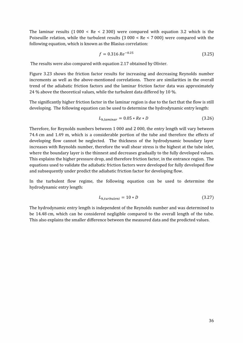
36
The laminar results (1 000 < Re < 2 300) were compared with equation 3.2 which is the
Poiseuille relation, while the turbulent results (3 000 < Re < 7 000) were compared with the
following equation, which is known as the Blasius correlation:
(3.25)
The results were also compared with equation 2.17 obtained by Olivier.
Figure 3.23 shows the friction factor results for increasing and decreasing Reynolds number
increments as well as the above-mentioned correlations. There are similarities in the overall
trend of the adiabatic friction factors and the laminar friction factor data was approximately
24 % above the theoretical values, while the turbulent data differed by 10 %.
The significantly higher friction factor in the laminar region is due to the fact that the flow is still
developing. The following equation can be used to determine the hydrodynamic entry length:
(3.26)
Therefore, for Reynolds numbers between 1 000 and 2 000, the entry length will vary between
74.4 cm and 1.49 m, which is a considerable portion of the tube and therefore the effects of
developing flow cannot be neglected. The thickness of the hydrodynamic boundary layer
increases with Reynolds number, therefore the wall shear stress is the highest at the tube inlet,
where the boundary layer is the thinnest and decreases gradually to the fully developed values.
This explains the higher pressure drop, and therefore friction factor, in the entrance region. The
equations used to validate the adiabatic friction factors were developed for fully developed flow
and subsequently under predict the adiabatic friction factor for developing flow.
In the turbulent flow regime, the following equation can be used to determine the
hydrodynamic entry length:
(3.27)
The hydrodynamic entry length is independent of the Reynolds number and was determined to
be 14.48 cm, which can be considered negligible compared to the overall length of the tube.
This also explains the smaller difference between the measured data and the predicted values.

37
FIGURE 3.23: VALIDATION OF ADIABATIC FRICTION FACTOR RESULTS INSIDE THE SMOOTH TUBE
The friction factor for the roughened tube was validated by considering approximately 83 data
sets with 100 data points each for each tube. The average of the increasing and decreasing
increments of Reynolds numbers between 500 and 7 000 were used to ensure that the laminar
and turbulent flow regimes are covered. These measurements were also made without any heat
transfer to eliminate the effect of varying viscosity and density.
The laminar results (400 < Re < 2 300) were compared with the Poiseuille equation again, while
the turbulent results (3 000 < Re < 7 000) were compared with equation 3.4, which is the
Modified Colebrook equation. Three different relative roughnesses were used for the
validation. The Moody Chart covers a relative roughness range between 0.00001 and 0.05;
therefore the relative roughness of this tube is not covered, although a theoretical line has been
included.
Figure 3.24 shows the friction factor results for increasing and decreasing Reynolds number
increments as well as the above-mentioned correlations. Although the data do not exactly
correlate with the existing correlations, there are similarities in the overall trend of the
adiabatic friction factors. It was expected that the laminar friction factors would be the same as
the smooth tube data and therefore slightly higher than the 64/Re correlation, since the laminar
friction factor is usually a function of the Reynolds number only and subsequently independent
of surface roughness in the laminar region. However, this was not the case and there was a
significant increase. In the turbulent region, the friction factor is strongly influenced by any
irregularity or roughness on the surface that disturbs the laminar sub layer and therefore
affects the flow. Since the relative roughness of this tube was higher than the maximum
relative roughness covered in the Moody Chart, it may be possible that the laminar flow was
also affected by the roughness, which explains the higher laminar friction factors. The
significantly higher turbulent friction factors may be due to the fact that a maximum relative

38
roughness of 0.05 was used for the Modified Colebrook equation, and therefore the current
relative roughness falls outside the boundaries.
FIGURE 3.24: VALIDATION OF ADIABATIC FRICTION FACTOR RESULTS INSIDE THE ROUGHENED TUBE
3.7.2 DIABATIC FRICTION FACTORS
The diabatic friction factors were validated in Figure 3.25 by using the results of the smooth
tube and comparing it with the measured data obtained by Olivier (2010) when he investigated
heat transfer through a 15.88 mm tube as well. However, for his experiments, a counterflow
tube-in-tube heat exchanger was used; therefore the boundary condition was constant wall
temperature instead of the constant heat flux boundary condition used for these experiments.
Since the boundary conditions are different, exact correlation with the data of Olivier cannot be
expected.
The measured data was also compared with the experimental data obtained by Ghajar (1997).
A square-edged inlet tube was used and the test fluid was an ethylene-glycol-water mixture.
Although this data was obtained when an 8 kW/m2 heat flux was applied, the exact correlation
with the 8.66 kW/m2 data cannot be expected, since the test fluids and therefore fluid
properties, differ.
Both increasing and decreasing increments of Reynolds numbers between 1 000 and 7 000
were used to ensure that the laminar and turbulent flow regimes were covered. Since the
increasing and decreasing Reynolds numbers data differed slightly, the average was used for the
validation.

39
The measured data correlates fairly well with the experimental data of Olivier and the overall
shape of the curves is similar. The friction factor data obtained when the 11.49 kW/m2 heat flux
were applied is higher than the adiabatic friction factors, although the friction factors obtained
when the other two heat fluxes were applied are significantly lower. This is not possible, since
the friction factors are suppose to increase due to the effect of secondary flow. The overall
shape of the curves are indeed correct and the transitional region is between Reynolds numbers
of 2 100 and 3 000. More detail on possible causes for the inaccurate friction factor data can be
found in Chapter 4. The experimental data of Ghajar shows that transition occurs significantly
later when an ethylene-glycol-water mixture is used instead of water.
FIGURE 3.25: VALIDATION OF DIABATIC FRICTION FACTOR INSIDE THE SMOOTH TUBE
3.7.3 HEAT TRANSFER COEFFICIENTS
The Nusselt numbers (or indirectly the heat transfer coefficients) of the smooth tube were
validated in Figure 3.26 by using the results of the smooth tube again. Approximately 100 data
sets with 100 data points each for each heat flux applied used. Both increasing and decreasing
increments of Reynolds numbers between 1 000 and 7 000 were used to ensure that the
laminar and turbulent flow regimes were covered. Since the increasing and decreasing
Reynolds numbers data differed slightly, the average was used for the validation. The measured
data was again compared to experimental data obtained by Olivier (2010) and Ghajar (1997).
The measured data in the turbulent region obtained with the 11.49 kW/m2 heat flux applied,
correlates well with the data of Olivier, although it was obtained from experiments using a
different boundary condition. Exact correlation is obtained in the turbulent region; however,
there is an 8 % and 12 % difference in the laminar and transitional regions, respectively.
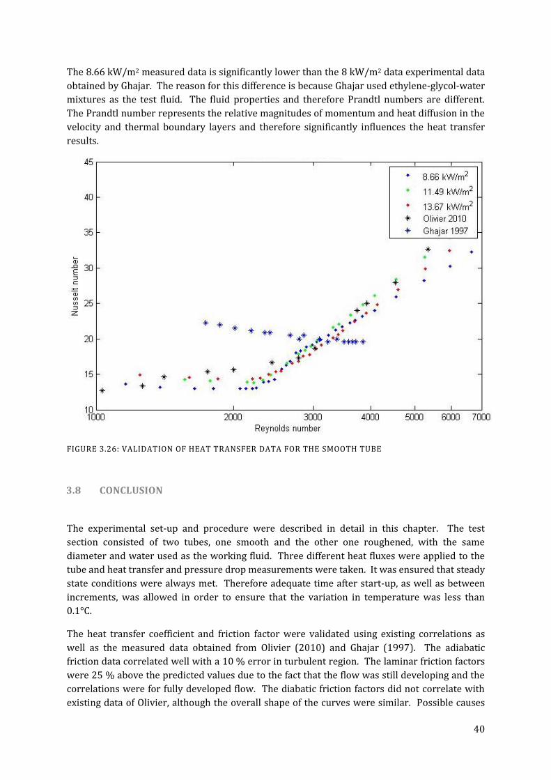
40
The 8.66 kW/m2 measured data is significantly lower than the 8 kW/m2 data experimental data
obtained by Ghajar. The reason for this difference is because Ghajar used ethylene-glycol-water
mixtures as the test fluid. The fluid properties and therefore Prandtl numbers are different.
The Prandtl number represents the relative magnitudes of momentum and heat diffusion in the
velocity and thermal boundary layers and therefore significantly influences the heat transfer
results.
FIGURE 3.26: VALIDATION OF HEAT TRANSFER DATA FOR THE SMOOTH TUBE
3.8 CONCLUSION
The experimental set-up and procedure were described in detail in this chapter. The test
section consisted of two tubes, one smooth and the other one roughened, with the same
diameter and water used as the working fluid. Three different heat fluxes were applied to the
tube and heat transfer and pressure drop measurements were taken. It was ensured that steady
state conditions were always met. Therefore adequate time after start-up, as well as between
increments, was allowed in order to ensure that the variation in temperature was less than
0.1°C.
The heat transfer coefficient and friction factor were validated using existing correlations as
well as the measured data obtained from Olivier (2010) and Ghajar (1997). The adiabatic
friction data correlated well with a 10 % error in turbulent region. The laminar friction factors
were 25 % above the predicted values due to the fact that the flow was still developing and the
correlations were for fully developed flow. The diabatic friction factors did not correlate with
existing data of Olivier, although the overall shape of the curves were similar. Possible causes

41
for the inaccuracies can be found in Chapter 4. An ethylene-glycol-water mixture was used as
the test fluid in the experiments done by Ghajar, which explains the significant difference
between the measured data and his experimental data.
Although there were slight differences between the measured heat transfer data and those
obtained by Olivier, the overall trend was similar and therefore the data has been validated.

42
4. RESULTS
4.1 INTRODUCTION
Two tubes, one smooth and the other with a relative roughness of 0.058, were investigated.
Both tubes were 1.8 m long and had outer diameters of 15.88 mm. The experimental results are
divided into two parts, namely the heat transfer results for the smooth tube and then a
comparison of the two tubes. The adiabatic friction factor results are included in the diabatic
friction factor results using 0 kW/m2. Solid markers are used to indicate the measured data for
the smooth tube, while crosses are used for the roughened tube.
4.2 SMOOTH TUBE
The Reynolds number was varied between 1 000 and 7 000 since transition was expected to
occur at a Reynolds number of approximately 2 300. This ensured that the whole transitional
region, as well as part of the laminar and turbulent region, was covered. Approximately 100
data sets with 100 data points each for each heat flux applied used. The average of the
increasing and decreasing increments of Reynolds numbers was used in the graphs.
4.2.1 FRICTION FACTORS
Figure 4.2 contains the experimental friction factors of the smooth tube against Reynolds
number. In the adiabatic case, transition from laminar to turbulent flow started at a Reynolds
number of approximately 2 100 and ended at approximately 2 400, which corresponds to the
transitional region at Reynolds numbers of 2 100 – 2 300, which appears in most fluid dynamics
textbooks. The s-curve of the diabatic friction factors was much smaller than for the adiabatic
case. Therefore it can be concluded that there is very little increase in friction factor in this
region.
It is important to investigate the diabatic friction factors, since the viscosity difference between
the bulk fluid and the fluid at the wall, as well as the effect of secondary flow, influences the
friction factors. From the diabatic friction factor data it follows that the friction factors obtained
when the 8.66 kW/m2 heat flux was applied, is significantly larger than the adiabatic and other
diabatic friction factors. The increase between the adiabatic and diabatic friction factors,
especially in the laminar region, may be due to secondary flow, which usually occurs in
horizontal heated tubes. The fluid near the tube wall has a higher temperature and lower
density and circulates upward, while the fluid in the centre circulates downward due to the
lower temperature and higher density. The temperature difference therefore creates secondary
flow due to free convection. Mixed convection (a combination of free convection due to
secondary flow and forced convection due to the heat flux applied) changes the velocity profile.
The friction factor is proportional to the wall shear stress, which in turn is proportional to the

43
velocity gradient at the wall. The velocity profile is affected in such a way that the velocity
gradient is much steeper at the tube wall. As the heat flux is increased, the shear stresses
increase due to the steeper velocity gradient, which leads to an increased friction factor.
Although the effect of heating is significant in the laminar and transitional regions, the heating
effect is almost negligible in the turbulent region. Secondary flow also influences the heat
transfer measurements in the laminar flow regime and the effect diminishes as the flow
becomes transitional and turbulent.
The influence of secondary flow is shown in Figure 4.1. There is a significant difference
between the top and bottom local heat transfer coefficients. These local heat transfer
coefficients were determined by using the temperature measurements at the top, bottom and
sides, respectively. The side local heat transfer coefficients were expected to be the same.
However, this is not the case and a possible reason may be that the tube was slightly turned
when it was connected to the rest of the experimental set-up.
FIGURE 4.1: LOCAL HEAT TRANSFER COEFFICIENTS FOR THE SMOOTH TUBE WHEN 8.66 KW/M2 HEAT FLUX APPLIED
The diabatic friction factors obtained when the 11.49 kW/m2 and 13.67 kW/m2 heat fluxes were
applied, in Figure 4.2, were unexpected since they are significantly lower than the adiabatic
friction factors, especially in the transitional region. The friction factors were determined using
equation 3.20; therefore they are dependent on the pressure drop, density, diameter and length
of tube as well as upon the velocity of the fluid. Since the tube dimensions, as well as the fluid
velocity and density are correct, the only variable that might be the reason for the incorrect data
is the pressure drop. The pressure drop was measured using a differential pressure transducer
and since both the pressure transducer and diaphragm have been used by previous students,
there is a possibility that it is slightly damaged or incorrect.
Another possibility may be that the diaphragm got damaged. This might well be the reason
since the adiabatic turbulent friction factors are only 10 % above the predicted values. The

44
adiabatic tests were done first and were then followed by the 8.66 kW/m2, 11.49 kW/m2 and
13.67 kW/m2 applied heat fluxes during the diabatic tests. From the results it can be observed
that the inaccuracy of the data increases with increasing heat fluxes, which confirms the
possibility of a damaged diaphragm. During each start-up of the system, the supply and by-pass
valves are adjusted in order to obtain maximum back pressure on the pump and therefore
reduce the flow pulsations. It is possible that the diaphragm may have been damaged during
this process when the pressure of the system was accidently increased significantly above the
calibrated pressure. The diaphragms are designed to withstand approximately two times their
maximum rated pressure before it break. A small diaphragm with a maximum pressure of
860 kPa was used for the smooth tube. Since the pressure was increased significantly above the
calibrated value of 580 kPa but not necessarily above 1.72 kPa, the diaphragm did not break,
but might got damaged and the calibration might have been less accurate for the rest of the
tests. A good safety measure for future experiments will therefore be to check and recalibrate
the diaphragms between tests if the pressure was accidently increased significantly above the
maximum pressure.
FIGURE 4.2: EXPERIMENTAL FRICTION FACTORS FOR THE SMOOTH TUBE AS A FUNCTION OF REYNOLDS NUMBER FOR DIFFERENT HEAT FLUXES
4.2.2 HEAT TRANSFER
In order to investigate the heat transfer, a graph of the Nusselt numbers against Reynolds
numbers was generated. From Figure 4.3 it can be concluded that transition is delayed for
increasing heat fluxes. Transition occurs approximately at 2 100 when 8.66 kW/m2 is applied
and at 2 200 and 2 400 when 11.49 kW/m2 and 13.67 kW/m2 are applied. In the laminar region,
the Nusselt number is higher for higher heat fluxes. In the transitional region, however, the

45
opposite is true and the gradient of transition is higher for higher heat fluxes. Therefore, the
gradient of transition is greater for higher heat fluxes.
The Nusselt numbers in the laminar region are significantly higher than the predicted
theoretical constant 4.36 for a constant heat flux boundary condition. These higher values are
due to the buoyancy-induced secondary flow in the tube which was caused by the difference in
density at the center and wall of the tube. The secondary flow influences forced convection and
causes mixed convection heat transfer.
The Nusselt numbers also increases with an increased heat flux applied from approximately 13
when the 8.66 kW/m2 heat flux is applied, to approximately 14 when the 13.67 kW/m2 heat flux
is applied in the laminar region. As the flow rate decreases in the laminar region, the Nusselt
numbers increases slightly. This may be due to increased heat loss through the insulation at
these low flow rates.
FIGURE 4.3: EXPERIMENTAL HEAT TRANSFER DATA FOR THE SMOOTH TUBE IN TERMS OF NUSSELT NUMBERS AGAINST REYNOLDS NUMBERS FOR DIFFERENT HEAT FLUXES
The effect of secondary flow in the laminar and transitional regions is shown in Figure 4.4
where to ratio of the heat transfer coefficients at the top and bottom of the tube is plotted. For
forced convection (in the absence of buoyancy effects), the ratio should be unity, while it should
be less than unity for mixed convection. From the figure it follows that the ratio of the local heat
transfer coefficients decrease for increasing heat fluxes applied. This trend is consistent with
the effect of secondary flow that increases as the applied heat flux increases. As the Reynolds
number increases, the ratio of the local heat transfer coefficients approaches unity in the upper
bound of the transition region. Therefore it can be concluded that the secondary flow effect is
significant in the laminar flow regime, decreases in the transitional regime and is suppressed by
the turbulent motion.

46
FIGURE 4.4: LOCAL HEAT TRANSFER RATIO FOR THE SMOOTH TUBE FOR DIFFERENT HEAT FLUXES APPLIED
The heat transfer results can also be plotted in terms of the Colburn j-factor, using equation 2.8,
since this account for the variation in the fluid Prandtl number. From Figure 4.5, it can be
confirmed that transition is delayed for increasing heat fluxes. Transition occurred at Reynolds
numbers between 2 200 and 2 800 when the 8.66 kW/m2 heat flux was applied, between 2 300
and 3 000 when the 11.49 kW/m2 heat flux was applied, and between 2 500 and 3 200 when the
13.67 kW/m2 heat flux was applied.

47
FIGURE 4.5: SMOOTH TUBE HEAT TRANSFER DATA IN TERMS OF THE COLBURN J-FACTORS FOR DIFFERENT HEAT FLUXES
4.3 ROUGHENED TUBE
The Reynolds numbers were varied between 500 and 7 000 in order to cover as large as
possible a section of the transitional and laminar flow regimes. This was not always possible
since, the experimental set-up was initially designed to operate at Reynolds numbers between
1 000 and 7 000 and a tube with a relative surface roughness of 0.001. However, as mentioned
in Chapter 3, there was not a significant difference between the result of this roughness and
those of the smooth tube. Therefore, the surface roughness was increased drastically which
caused transition to occur much earlier than expected. While the 13.67 kW/m2 heat flux was
applied, the water at the tube exit reached a maximum temperature of 72 °C and the tube
surface a maximum temperature of 95 °C at a Reynolds number of 500. Since the tube was
heated to 100 °C when the thermocouples were soldered to the tube, it was undesirable to heat
the tube above 95 °C because the thermocouples might loosen again. Therefore, this limited the
system from operating at lower Reynolds numbers.
4.3.1 FRICTION FACTORS
The friction factor is strongly influenced by the surface roughness, as shown in Figure 4.6. The
laminar sub layer is disturbed by irregularities or roughness on the surface and flow is
therefore affected. The friction factors are strongly influenced by the surface roughness in the
turbulent region, and this effect is minimal in the laminar region.
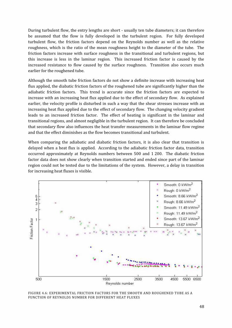
48
During turbulent flow, the entry lengths are short - usually ten tube diameters; it can therefore
be assumed that the flow is fully developed in the turbulent region. For fully developed
turbulent flow, the friction factors depend on the Reynolds number as well as the relative
roughness, which is the ratio of the mean roughness height to the diameter of the tube. The
friction factors increase with surface roughness in the transitional and turbulent regions, but
this increase is less in the laminar region. This increased friction factor is caused by the
increased resistance to flow caused by the surface roughness. Transition also occurs much
earlier for the roughened tube.
Although the smooth tube friction factors do not show a definite increase with increasing heat
flux applied, the diabatic friction factors of the roughened tube are significantly higher than the
adiabatic friction factors. This trend is accurate since the friction factors are expected to
increase with an increasing heat flux applied due to the effect of secondary flow. As explained
earlier, the velocity profile is disturbed in such a way that the shear stresses increase with an
increasing heat flux applied due to the effect of secondary flow. The changing velocity gradient
leads to an increased friction factor. The effect of heating is significant in the laminar and
transitional regions, and almost negligible in the turbulent region. It can therefore be concluded
that secondary flow also influences the heat transfer measurements in the laminar flow regime
and that the effect diminishes as the flow becomes transitional and turbulent.
When comparing the adiabatic and diabatic friction factors, it is also clear that transition is
delayed when a heat flux is applied. According to the adiabatic friction factor data, transition
occurred approximately at Reynolds numbers between 500 and 1 200. The diabatic friction
factor data does not show clearly when transition started and ended since part of the laminar
region could not be tested due to the limitations of the system. However, a delay in transition
for increasing heat fluxes is visible.
FIGURE 4.6: EXPERIMENTAL FRICTION FACTORS FOR THE SMOOTH AND ROUGHENED TUBE AS A FUNCTION OF REYNOLDS NUMBER FOR DIFFERENT HEAT FLUXES
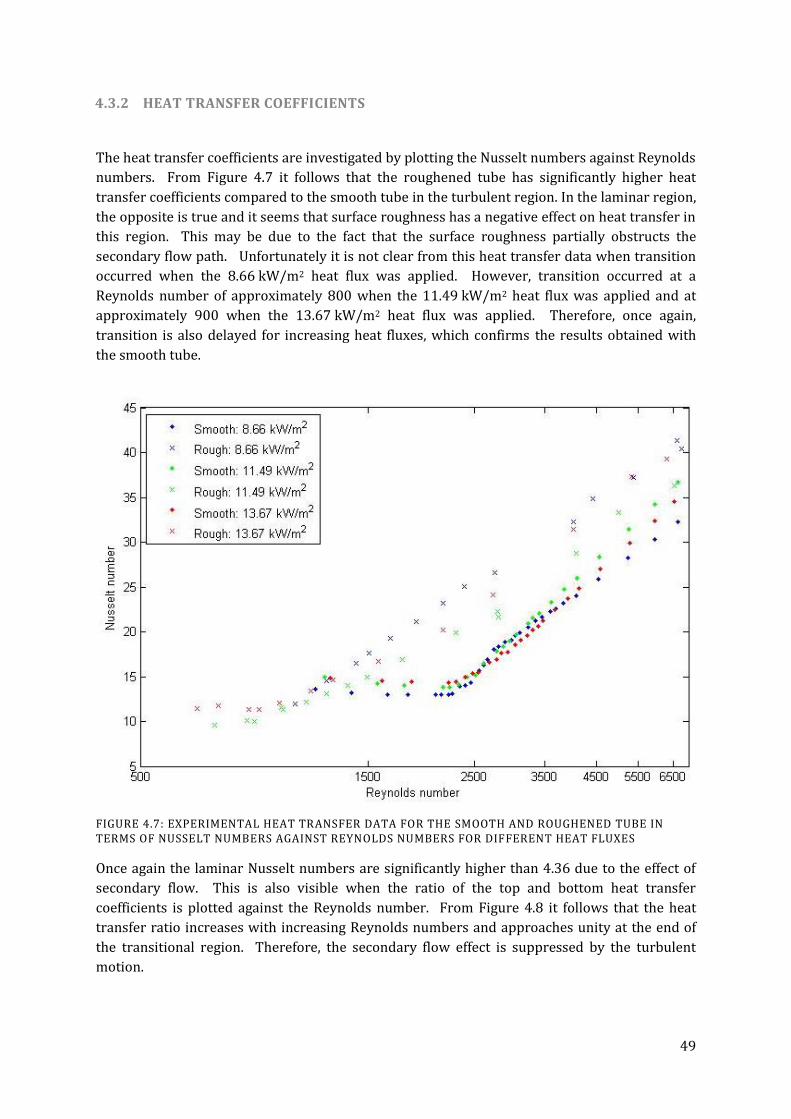
49
4.3.2 HEAT TRANSFER COEFFICIENTS
The heat transfer coefficients are investigated by plotting the Nusselt numbers against Reynolds
numbers. From Figure 4.7 it follows that the roughened tube has significantly higher heat
transfer coefficients compared to the smooth tube in the turbulent region. In the laminar region,
the opposite is true and it seems that surface roughness has a negative effect on heat transfer in
this region. This may be due to the fact that the surface roughness partially obstructs the
secondary flow path. Unfortunately it is not clear from this heat transfer data when transition
occurred when the 8.66 kW/m2 heat flux was applied. However, transition occurred at a
Reynolds number of approximately 800 when the 11.49 kW/m2 heat flux was applied and at
approximately 900 when the 13.67 kW/m2 heat flux was applied. Therefore, once again,
transition is also delayed for increasing heat fluxes, which confirms the results obtained with
the smooth tube.
FIGURE 4.7: EXPERIMENTAL HEAT TRANSFER DATA FOR THE SMOOTH AND ROUGHENED TUBE IN TERMS OF NUSSELT NUMBERS AGAINST REYNOLDS NUMBERS FOR DIFFERENT HEAT FLUXES
Once again the laminar Nusselt numbers are significantly higher than 4.36 due to the effect of
secondary flow. This is also visible when the ratio of the top and bottom heat transfer
coefficients is plotted against the Reynolds number. From Figure 4.8 it follows that the heat
transfer ratio increases with increasing Reynolds numbers and approaches unity at the end of
the transitional region. Therefore, the secondary flow effect is suppressed by the turbulent
motion.

50
FIGURE 4.8: LOCAL HEAT TRANSFER RATIO FOR THE ROUGHENED TUBE FOR DIFFERENT HEAT FLUXES APPLIED
The heat transfer results were also plotted in terms of the Colburn j-factor in Figure 4.9 in order
to account for the variation in the fluid Prandtl number. Similar to the Nusselt number results,
the Colburn j-factor is higher for lower heat fluxes in the turbulent region. Transition was
slightly delayed for higher heat fluxes since it started at a Reynolds number of approximately
800 when the 11.49 kW/m2 heat flux was applied and at approximately 900 when the
13.67 kW/m2 heat flux was applied. This confirms the conclusions made from the heat transfer
data in terms of the Nusselt number. Unfortunately it is not clear from Figure 4.9 where
transition occurred when the 8.66 kW/m2 heat flux was applied.

51
FIGURE 4.9: EXPERIMENTAL DATA FOR THE SMOOTH TUBE IN TERMS OF THE COLBURN J-FACTOR
4.4 CONCLUSION
The friction factor results of the smooth tube were inconsistent and therefore inaccurate, since
the diabatic friction factors decreased for increasing heat fluxes applied. It also showed that
transition is not delayed for increasing heat fluxes applied. The friction factors are dependent
on the pressure drop, density, diameter and length of tube as well as the velocity of the fluid.
Since the tube dimensions - as well as the fluid velocity and density - are correct, the only
variable that could account for the incorrect data is the pressure drop. The pressure drop was
measured using a differential pressure transducer and a diaphragm which was selected
according to the pressure drop range that was tested. The inaccuracy between the adiabatic
and diabatic data increased drastically which implies that the diaphragm might have been
damaged.
A different diaphragm was used for the roughened tube, because the pressure drop was much
higher. Since the inaccuracy of the friction factor data for the roughened tube was significantly
less than for the smooth tube, it is confirmed that a damaged diaphragm is the reason for the
inaccurate friction factor results of the smooth tube.
The adiabatic friction factor data revealed that transition occurred approximately at Reynolds
numbers between 500 and 1 200, which is significantly earlier than the transition of the smooth
tube which occurred between Reynolds numbers of 2 100 and 2 800. The diabatic friction
factor data does not clearly show when transition started and ended since part of the laminar
52
region could not be tested due to the limitations of the system. However, a delay in transition
for increasing heat fluxes is visible
The heat transfer results of the smooth tube show that transition occurs approximately at 2 100
when 8.66 kW/m2 is applied and at 2 200 and 2 300 when 11.49 kW/m2 and 13.67 kW/m2 is
applied. In the laminar region, the Nusselt number is higher for higher heat fluxes. However, in
the transitional region, the opposite is true and the gradient of transition is higher for higher
heat fluxes. The laminar Nusselt numbers were higher than the predicted theoretical constant
4.36 for a constant heat flux boundary condition, due to the buoyancy-induced secondary flow
in the tube which was caused by the difference in density at the center and wall of the tube. The
secondary flow disturbs the velocity boundary layer in such a way that the shear stress and
therefore friction coefficient is increased. The Colburn j-factor plots confirmed that transition is
delayed and that the heat transfer increases for increasing heat fluxes.
The roughened tube has significantly higher turbulent heat transfer coefficients, compared to
the smooth tube. However, the opposite is true in the laminar region and it can therefore be
concluded that surface roughness has a negative effect on heat transfer at low flow rates. This
may be due to the fact that the surface roughness partially obstructs the secondary flow path.
Transition is also delayed for increasing heat fluxes, since it started at a Reynolds number of
approximately 800 when the 11.49 kW/m2 heat flux was applied and at approximately 900
when the 13.67 kW/m2 heat flux was applied. Unfortunately it is not clear where transition
occurred when the 8.66 kW/m2 heat flux was applied.
Due to inaccurate friction factor data of the smooth tube and incomplete friction factor data of
the roughened tube, it is not possible to develop correlations to accurately describe the
influence of surface roughness in the transitional flow regime. The exact boundaries of the
transitional flow regime could not be determined since a sufficient part of the laminar region
could not be covered due to the limitations of the experimental set-up.

53
4. CONCLUSION AND RECOMMENDATIONS
Heat exchangers are usually designed to operate in either the laminar or the turbulent flow
regime, while the transitional flow regime is avoided due to uncertainties and irregularities. Up
to now the transitional flow regime has been investigated, however, there has been no previous
work done on influence of surface roughness in the transitional flow regime.
An experimental set-up was built in order to investigate the influence of surface roughness on
the heat transfer and pressure drop performance. The system consisted of a smooth and
roughened tube, both with an outer diameter and length of 15.88 mm and 1.8 m, respectively.
The type of inlet was square-edged and water was used as the test fluid. The roughened tube
was roughened by gluing sand grains with an average size of 0.84 mm to the inside surface of
the copper tube and the tube therefore had a relative roughness of 0.058.
A total of 810 data sets, each with 100 data points captured at a frequency of 10 Hz, were used
to generate 44 graphs which were used to investigate the influence of surface roughness. The
adiabatic friction factor results showed that surface roughness increases the friction factor and
that transition occurred earlier as well. The diabatic friction factors for the smooth tube were
inaccurate due to a damaged diaphragm in the pressure transducer. A different diaphragm was
used for the roughened tube, because the pressure drop was significantly higher and since the
inaccuracy of these results were significantly less, it was confirmed that the diaphragm used for
the smooth tube had been damaged.
The adiabatic friction factor data revealed that transition occurred approximately at Reynolds
numbers between 500 and 1 200, which is significantly earlier than the transition of the smooth
tube which occurred between Reynolds numbers of 2 100 and 2 800. The diabatic friction
factor data does not show clearly when transition started and ended since part of the laminar
region could not be tested due to the limitations of the system. However, a delay in transition
for increasing heat fluxes is visible.
The heat transfer results of the smooth tube shows that transition occurs approximately at
2 100 when 8.66 kW/m2 is applied and at 2 200 and 2 300 when 11.49 kW/m2 and
13.67 kW/m2 is applied. Transition for the roughened tube started at a Reynolds number of
approximately 800 when the 11.49 kW/m2 heat flux was applied and at approximately 900
when the 13.67 kW/m2 heat flux was applied. Unfortunately it is not clear where transition
occurred when the 8.66 kW/m2 heat flux was applied. However, it can be concluded that
transition is delayed for increasing Reynolds numbers. The laminar Nusselt numbers of both
tubes were higher than the predicted theoretical constant 4.36 for a constant heat flux boundary
condition, due to the buoyancy-induced secondary flow in the tube which was caused by the
difference in density at the center and wall of the tube. The Nusselt numbers for the roughened
tube were lower than for the smooth tube in the laminar region, but the opposite was true in the
turbulent region. These lower Nusselt numbers may be due to the surface roughness which
disrupted the secondary flow path and reduced the amount of mixing. Secondary flow also
increased the diabatic friction factors, especially in the laminar region, since it increases the
wall shear stress and therefore the overall pressure drop. The effect of secondary flow was
almost negligible in the turbulent region.

54
The Colburn j-factors in the transitional flow regime were higher for increasing heat fluxes in
both the smooth and roughened tube, although those in the roughened tube were significantly
higher than in the smooth tube. This confirms that surface roughness increases the heat
transfer in the transitional flow regime.
Unfortunately, due to inaccurate friction factor data for the smooth tube, and incomplete friction
factor data for the roughened tube, correlations could not be developed to describe the
influence of surface roughness in the transitional flow regime. It was also not possible to
determine the boundaries of the transitional flow regime, since a sufficient part of the laminar
flow region could not be covered for the roughened tube due to the limitations of the
experimental set-up.
It is therefore recommended that future work should include the following:
An experimental set-up that is designed to operate at very low Reynolds numbers to
accurately cover the whole transitional flow regime, as well as part of the laminar and
turbulent flow regimes.
The measurement equipment, for example the pressure transducers, should be verified
between tests to ensure that it is not damaged or inaccurate.
Although an extensive amount of tests had been performed, a large database is required
in order to accurately describe transition; therefore it would be advisable to investigate
more heat fluxes and finer increments, especially during tests with the roughened tube.
Water was the only test fluid used. Different fluids (with different Prandtl numbers), for
example an ethylene-glycol-water mixture, should, however, also be tested in order to
determine the influence of the Prandtl number.
A range of diameters, of tubes with the same surface roughness, should be investigated.
The tube was roughened by gluing sand grains to the inner surface of the copper tube.
Although an experiment showed that the influence of the sand grains and glue has a
negligible effect on the heat transfer, the accuracy of the results will be improved by
roughening the tube with a similar material to that of the tube itself.
A wider range of surface roughness can also be investigated in order to accurately
determine its influence.
55
5. REFERENCES
ASHRAE,2009. Fluid Flow, ASHRAE Handbook – Fundamentals, American Society of Heatin,
Refrigerating and Air-Conditioning Engineers, Inc., Atlanta
Cengel, Y. A., 2006. Heat and Mass Transfer. 3rd ed., Singapore: McGraw-Hill.
Ghajar, A. J., and Madon, K. F., Pressure Drop Measurements and Correlations in the Transition
Region for a Circular Tube with Three Different Inlet Configurations. Experimental Thermal
Fluid Science. 5, 129-135, 1992.
Ghajar, A. J., and Tam, L. M., Flow Regime Map for a Horizontal Pipe with Uniform Wall Heat Flux
and Three Inlet Configurations. Experimental Thermal Fluid Science. 10, 287-297, 1995.
Ghajar, A. J., and Tam, L. M., Heat Transfer Measurements and Correlations in the Transition
Region for a Circular Tube with Three Different Inlet Configurations. Experimental Thermal
Fluid Science. 8, 79-90, 1994.
Ghajar, A. J., and Tam, L. M., Effect of Inlet Geometry and Heating on the Fully Developed Friction
Factor in the Transition Region of a Horisontal Tube. Experimental Thermal Fluid Science. 15,
52-64, 1997.
Meyer, J.P. and Olivier, J.A., Heat Transfer in the Transitional Flow Regime. Evaporation,
Condensation and Heat Transfer, InTech, pp. 245-260, 2011.
Meyer, J.P. and Olivier, J.A., Single-Phase Heat Transfer and Pressure Drop of the Cooling Water
inside Smooth Tubes for Transitional Flow with Different Inlet Geometries. HVAC&R Research,
16(4), pp. 471-496, 2010.
Meyer, J.P. and Olivier, J.A., Transitional Flow inside enhanced tubes for fully developed and
developing flow with different types of inlet disturbances: Part 1 - Adiabatic Pressure Drops.
International Journal for Heat and Mass Transfer. 54, 1587-1597, 2010
Meyer, J.P. and Olivier, J.A., Transitional Flow inside enhanced tubes for fully developed and
developing flow with different types of inlet disturbances: Part 2 - heat transfer. International
Journal for Heat and Mass Transfer. 54 ,1598-1607, 2010
Mkhontho, E., Flow in the Transitional Flow Regime, Final Year Project, Department of Mechanical and Aeronautical Engineering, University of Pretoria, 2011.
Obot, N.T., Esen, E.B., Rabas, T.J., The role of transition in determining friction and heat transfer
in smooth and rough passages. International Journal of Heat and Mass Transfer, 33,2133-2143,
1990.
Olivier, J.A., Single-Phase Heat Transfer and Pressure Drop of Water Cooled at a Constant Wall
Temperature Inside Horizontal Circular Smooth and Enhanced Tubes with Different Inlet
Configurations in the Transitional Flow Regime, Ph.D. Thesis, Department of Mechanical and
Aeronautical Engineering, University of Pretoria, 2009.

56
Omega. 2012. Product Spec Sheet. [Online]. Available:
http://www.omega.co.uk/ppt/pptsc.asp?ref=FINEWIRE_DUPINSUL [2012, March,18]
Toprak,H. 2006. Waste Water Engineering. [Online]. Avalaible:
http://web.deu.edu.tr/atiksu/enter.html [2012,October,15]
White, F., 2009. Fluid Mechanics. 6th ed. Singapore: McGraw-Hill

A.1
APPENDIX A: SURFACE ROUGHNESS
Appendix A contains the results of the surface roughness measurements which was done by
Metlab, as well as the results of the grading analysis.

I I
,_
.-,,,,
,57
Char
!C,llI
ers
Stre
etBo
ksbu
rgNo
rthr---
:T::E:-
::S::T=
-=R-=E
-=P~O
:-:R::T:
-:":'I
N7""":
'A'::::C
~C:-:O
~R:-::D
::"A":':"
":N-=C
-=E:-:W
":":":IT
::H"':""
=E~N
~1:-:O
~2:-:0~
4-:3~.1
':"""':::O
~F:-:S
::"A~M
:-:::P-:
-L-=E
~A:-:S
::"'::::S
-:-U:-::P
:-::P:7L
7.1E=
D=---:
(Ii:--~~
IIII~~:J
l'PO
Box
1028
,Bo
ksbu
rg,
1460
......
.7""
"'-~Te
J(01
1)91
7517
3·Fa
x(0
11)
917
0546
Cus
tom
er:
Uni
vers
ityof
Pre
toria
Mat
eria
lsp
ecifi
catio
n:C
oppe
r--
IEm
ali.m
etlab
@te
lkom
sa.n
el
Ord
erno
:C
OD
I"M
E'T
LA
B._._
webs
ite,.W
NW.m
etlab
.co.za
Add
ress
:P
OB
ox39
814
IfI
Dire
ctor
TCW
Brink
(Pr.l
ng/E
ng.)
Mor
elet
aP
ark
Des
crip
tion:
15m
mO
Dtu
bes
I44
ITe
leph
one:
0129
9702
96R
EPO
RT
NU
MB
ER:
12-
3427
AE
mai
l:m
ever
ts(Q
)mw
eb.c
o.za
Dat
eR
ecei
ved:
Dat
ete
sted
:A
ttent
ion:
Mar
ilize
Eve
rtsId
entif
icat
ion:
See
belo
w25
1Jun
e20
1226
June
2012
*N
ota
SA
NA
Sac
cred
ited
activ
ity
SU
RFA
CE
RO
UG
HN
ES
SM
EA
SU
RE
ME
NTS
*S
ampl
eR
a[u
rn]
Rz
[urn
]Lo
ngro
ugh
0.42
40.
406
0.36
16.
084
5.36
04.
935
Sho
rtro
ugh
1.67
01.
674
1.65
614
.560
14.0
3013
.930
Sm
ooth
0.03
30.
036
0.03
80.
455
0.46
30.
508
Sur
face
roug
hnes
sm
easu
rem
ents
perfo
rmed
onin
tern
alsu
rface
sof
tube
s.
/1
Tes
tsre
ques
ted,
inac
cord
ance
with
spec
.pr
ovid
edfIM
~T
ests
requ
este
d,no
tin
acco
rdan
cew
ithsp
ec.
prov
ided
121-~~
1tc.-
I
.-[
~r~IY
i'''''
No
requ
irem
ents
prov
ided
Xf,4
:",
,I,.
J11
.o,.,
OL
RE
MA
RK
S:
WIT
NE
SS
BY
:M
AN
AG
EM
EN
T11
I:~
)il~'4v
"CUi
TEG
HN
ICL
,,-'-'
-'N
/AS
IGN
ATO
RY
SIG
NA
TOR
YTE
STI
NG
WA
SC
AR
RIE
DO
UT
INA
CC
OR
DA
NC
EW
ITH
THE
FOLL
OW
ING
ME
TLA
BP
RO
CE
DU
RE
S(S
uppo
rting
inle
mat
iona
lpr
oced
ures
):M
EC
H30
,33
,34
s39
(AS
TMA
370;
E8;
E21
;IS
O68
92M
etho
d6;
EN
1000
2·5)
ME
CH
31&
32
(AS
TMA
370;
E23
;B
SE
N10
045-
1)M
ET
01(A
STM
E92
;E
384)
ME
T02
(AS
TME
10;
A37
0)M
ET0
3(A
STM
E18
;A
370)
ME
T04
(AS
TMB
117)
ME
T05
(AS
TMA
255;
E18
)M
ET0
6(A
STM
E10
77)
ME
T07
(AS
TME
340;
E38
1)M
ET0
8(A
STM
E3;
A26
2)M
ET0
9(A
STM
E3;
E45
)M
ET1
0(A
STM
E3;
E45
)M
ET1
1(A
STM
E3;
E45
;E
112;
E40
7)M
ET1
3(A
STM
B49
9)M
ET1
4(A
STM
6487
)M
ET
16(A
STM
E11
0)E
110,
CH
EM
S70
s71
(AS
TME
415)
CH
EM
A54
(AS
TME
1019
)
Paa
e1
of1
•..•••.•..•••.••
nri't"'•..••
n~
ro""
""",,
..,,t
•..••,
..••r
,..n
.r.+
•••.
•.,.+,.
.<"
•.•.•.••••
•••••••
"r•..•.••..'
•..•
n J

~
MET
lAB
(PTY
)LTD
·RE
G.#9
5113
8261
07
57Ch
artC
iJlier
sStre
et,
Boks
burg
North
TES
TR
EP
OR
TIN
AC
CO
RD
AN
CE
WIT
HE
N10
2043
.1O
FS
AM
PLE
AS
SU
PP
LIE
DPO
Box
1028
.Bok
sbur
g,14
60Te
l:(01
1)91
751
73·
Fax
(011
)917
0546
Cus
tom
er:
Uni
vers
ityof
Pre
toria
Mat
eria
lsp
ecifi
catio
n:C
oppe
r
1MEm
ailm
etlab
@te
lkom
sa.n
et
Ord
erno
:C
OD
ET
LA
B_
__
_~e
bsi~
wwwm
etlab
.co.za
Add
ress
:P
OB
ox39
814
Dire
ctor'le
WBr
ink(P
r.lng
IEng
.)
Mor
elet
aP
ark
Des
crip
tion:
±01
6mm
x0.
7mm
wal
ltu
be
44A
ctua
lpi
pe(s
hort)
Tele
phon
e:01
2997
0296
RE
PO
RT
NU
MB
ER
:12
-377
8A
Em
ail:
mev
erts
@m
web
.co.
zaD
ate
Rec
eive
d:D
ate
test
ed:
Atte
ntio
n:M
arili
zeE
verts
Iden
tific
atio
n:S
ampl
eA
12,J
uly
2012
13Ju
ly20
12
SU
RFA
CE
RO
UG
HN
ES
SM
EA
SU
RE
ME
NTS
*R
a(u
rn)
Rz
(urn
)S
ampl
e2.
039
I2.
087
I2.
091
12.5
7I
12.6
4I
12.6
5S
urfa
cero
ughn
ess
mea
sure
men
tspe
rform
edon
inte
rnal
surfa
ces
oftu
bes.
*N
ota
SA
NA
Sac
cred
ited
activ
ity
No
requ
irem
ents
prov
ided
,XR
EM
AR
KS
:W
ITN
ES
SB
Y:
N/A
MA
NA
GE
ME
NT
SIG
NA
TOR
Y
Test
sre
ques
ted,
inac
cord
ance
with
spec
.pr
ovid
ed
Test
sre
ques
ted,
not
inac
cord
ance
with
spec
.pr
ovid
ed
Pag
e1
of1
TES
TIN
GW
AS
CA
RR
IED
OU
TIN
AC
CO
RD
AN
CE
WIT
HTH
EFO
LLO
WIN
GM
ETL
AB
PR
OC
ED
UR
ES
(Sup
porti
ngin
tern
atio
nal
proc
edur
es):
ME
CH
30,
33,
34&
39(A
STM
A37
0;E
a;E
21;
ISO
6892
Met
hod
B;
EN
1000
2-5)
ME
CH
31&
32(A
STM
A37
0;E
23;
6SE
N10
045-
1)M
ET
01(A
STM
E92
;E
384)
ME
T02
(AS
TME
l0;
A37
0)M
ET0
3(A
STM
E18
;A
370)
ME
T04
(AS
TM61
17)
ME
T05
(AS
TMA
255;
E18
)M
ET0
6(A
STM
El0
77)
ME
T07
(AS
TME
340;
E38
1)M
ET0
8(A
STM
E3;
A26
2)M
ET0
9(A
STM
E3;
E45
)M
ET1
0(A
STM
E3;
E45
)M
ETl
l(A
STM
E3;
E45
;E
l12;
E40
7)M
ET1
3(A
STM
6499
)M
ET1
4(A
STM
6487
)M
ET
16(A
STM
Ell0
)E
ll0,
CH
EM
S70
&71
(AS
TME
415)
CH
EM
A54
(AS
TME
l019
)-
r'ti
,...
tt
i.o.rlif'
tArt:n
0.
Ci

I
.~
MET
LAB
(PTY
)LTD
·RE
G.#95/13826/07
I i57
Char
!Cilli
ers
Stre
et,
Boks
burg
North
TES
TR
EP
OR
TIN
AC
CO
RD
AN
CE
WIT
HE
N10
2043
.1O
FS
AM
PLE
AS
SU
PP
LIE
DPO
Box
1028
.Bok
sbur
g,14
60Te
l(01
1)91
751
73·
Fax
(011
)917
0546
Cus
tom
er:
Uni
vers
ityof
Pre
toria
Mat
eria
lsp
ecifi
catio
n:C
oppe
r
~
:met
lab@
telko
msa
.nel
Ord
erno
:C
OD
IE
TL
AB
__
__~~
~~
~~
__
wwwr
nena
b.co
.zaI
PO
Box
3981
4,
Add
ress
:Di
recto
r:TC
WBr
ink(P
r.lng
/Eng
.)
Mor
elet
aP
ark
Des
crip
tion:
±01
6mm
x0.
7mm
wal
ltu
be
44M
iddl
epi
pe(lo
ng)
Tele
phon
e:01
2997
0296
RE
PO
RT
NU
MB
ER
:12
-377
8B
Em
ail:
mev
erts
@m
web
.co.
zaI
Dat
eR
ecei
ved:
Dat
ete
sted
:A
ttent
ion:
Mar
ilize
Eve
rtsId
entif
icat
ion:
Sam
ple
B12
July
2012
13Ju
ly20
12
SU
RFA
CE
RO
UG
HN
ES
SM
EA
SU
RE
ME
NTS
*
II
Ra
(urn
)R
z(u
m)
Sam
ple
I2.
0311
I2.
034
I2.
052
13.9
5I
12.5
1I
12.3
5S
urfa
cero
ughn
ess
mea
sure
men
tspe
rform
edon
inte
rnal
surfa
ces
oftu
bes.
*N
ota
SA
NA
Sac
cred
ited
activ
ity
No
requ
irem
ents
prov
ided
xW
ITN
ES
SB
Y:
N/A
Tes
tsre
ques
ted,
inac
cord
ance
with
spec
.pr
ovid
ed
Tes
tsre
ques
ted,
not
inac
cord
ance
with
spec
.pr
ovid
ed
RE
MA
RK
S:
Pag
e1
of1
TES
TIN
GW
AS
CA
RR
IED
OU
TIN
AC
CO
RD
AN
CE
WIT
HTH
EFO
LLO
WIN
GM
ETL
AB
PR
OC
ED
UR
ES
(Sup
porti
ngin
tern
atio
nal
proc
edur
es):
ME
CH
30,
33,
34&
39(A
STM
A37
0;E
8;E
21;
ISO
6892
Met
hod
B;
EN
1000
2·S
)M
EC
H31
&32
(AS
TMA
370;
E23
;B
SE
N10
045·
1)M
ET
01(A
STM
E92
;E
384)
ME
T02
(AS
TME
10;
A37
0)M
Eli0
3(A
STM
E18
;A
370)
ME
T04
(AS
TM81
17)
ME
TOS
(AS
TMA
2SS
;E
18)
ME
T06
(AS
TME
1077
)M
ET0
7(A
STM
E34
0;E
381)
ME
T08
(AS
TME
3;
A26
2)M
ET0
9(A
STM
E3;
E4S
)M
ET1
0(A
STM
E3;
E4S
)M
ET1
1(A
STM
E3;
E4S
;E
112;
E40
7)M
ET1
3(A
STM
8499
)M
ET1
4(A
STM
B48
7)M
ET
16(A
STM
E11
0)E
110,
CH
EM
S70
&71
(AS
TME
41S
)C
HE
MA
S4
(AS
TME
1019
),.
•'..
+.
.•
c·
-


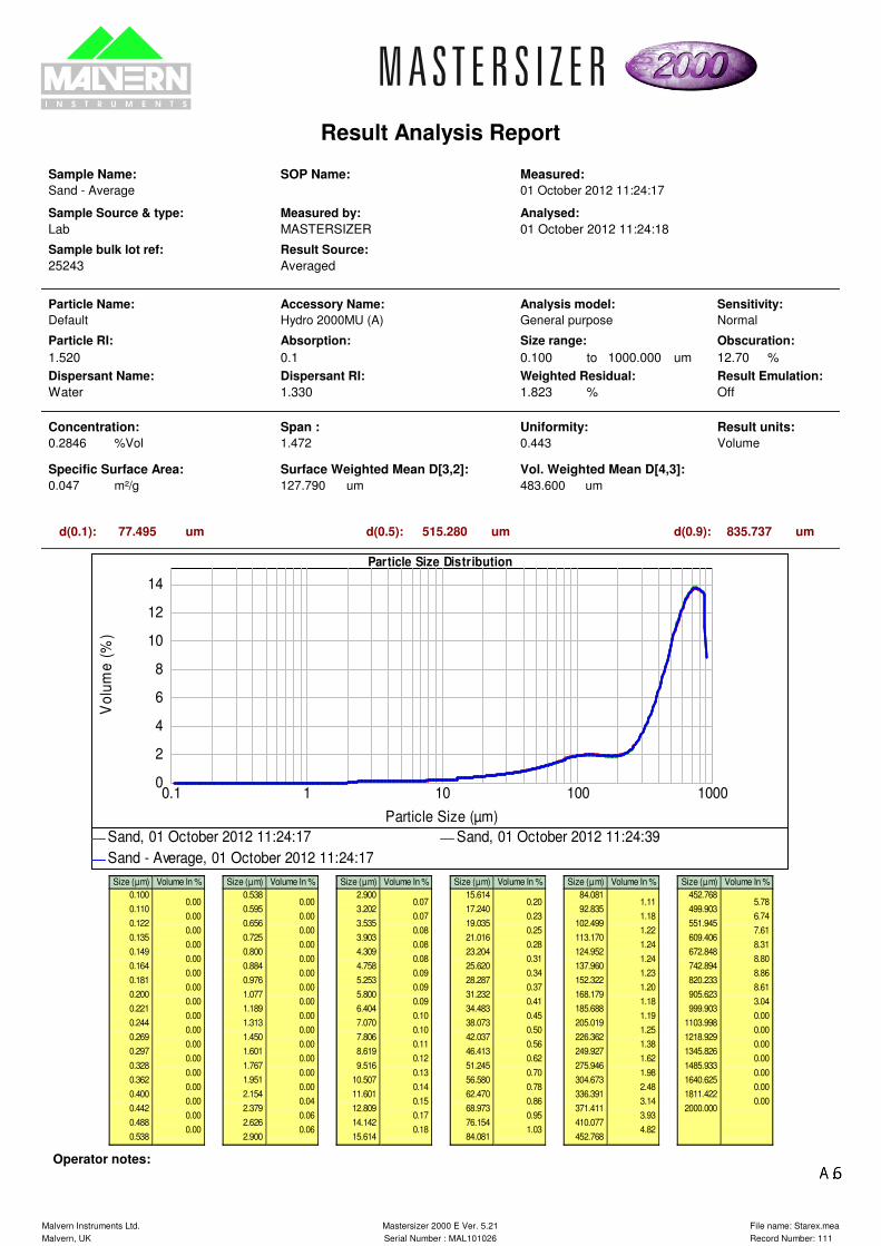
Result Analysis Report
Vol. Weighted Mean D[4,3]:
%
m²/g
um
Surface Weighted Mean D[3,2]:
0.047 483.600
d(0.9):
Accessory Name:
Span :
1.472
um
Specific Surface Area:
12.70
Operator notes:
Uniformity:
%Vol
Obscuration:
515.280 835.737d(0.1): um
0.443
127.790
um77.495 d(0.5):
Volume
Particle Size Distribution
0.1 1 10 100 1000
Particle Size (µm)
0
2
4
6
8
10
12
14
Vo
lum
e (
%)
Sand, 01 October 2012 11:24:17 Sand, 01 October 2012 11:24:39
Sand - Average, 01 October 2012 11:24:17
Hydro 2000MU (A)
Result units:
um
Concentration:
0.2846
Weighted Residual:
1.823 %
Size (µm)
0.100
0.110
0.122
0.135
0.149
0.164
0.181
0.200
0.221
0.244
0.269
0.297
0.328
0.362
0.400
0.442
0.488
0.538
Volume In %
0.00
0.00
0.00
0.00
0.00
0.00
0.00
0.00
0.00
0.00
0.00
0.00
0.00
0.00
0.00
0.00
0.00
Size (µm)
0.538
0.595
0.656
0.725
0.800
0.884
0.976
1.077
1.189
1.313
1.450
1.601
1.767
1.951
2.154
2.379
2.626
2.900
Volume In %
0.00
0.00
0.00
0.00
0.00
0.00
0.00
0.00
0.00
0.00
0.00
0.00
0.00
0.00
0.04
0.06
0.06
Size (µm)
2.900
3.202
3.535
3.903
4.309
4.758
5.253
5.800
6.404
7.070
7.806
8.619
9.516
10.507
11.601
12.809
14.142
15.614
Volume In %
0.07
0.07
0.08
0.08
0.08
0.09
0.09
0.09
0.10
0.10
0.11
0.12
0.13
0.14
0.15
0.17
0.18
Size (µm)
15.614
17.240
19.035
21.016
23.204
25.620
28.287
31.232
34.483
38.073
42.037
46.413
51.245
56.580
62.470
68.973
76.154
84.081
Volume In %
0.20
0.23
0.25
0.28
0.31
0.34
0.37
0.41
0.45
0.50
0.56
0.62
0.70
0.78
0.86
0.95
1.03
Size (µm)
84.081
92.835
102.499
113.170
124.952
137.960
152.322
168.179
185.688
205.019
226.362
249.927
275.946
304.673
336.391
371.411
410.077
452.768
Volume In %
1.11
1.18
1.22
1.24
1.24
1.23
1.20
1.18
1.19
1.25
1.38
1.62
1.98
2.48
3.14
3.93
4.82
Size (µm)
452.768
499.903
551.945
609.406
672.848
742.894
820.233
905.623
999.903
1103.998
1218.929
1345.826
1485.933
1640.625
1811.422
2000.000
Volume In %
5.78
6.74
7.61
8.31
8.80
8.86
8.61
3.04
0.00
0.00
0.00
0.00
0.00
0.00
0.00
01 October 2012 11:24:17
Averaged25243
Measured by:
MASTERSIZER
Sample bulk lot ref:
Lab
Sample Name:
Analysed:
Measured:
Sample Source & type:
01 October 2012 11:24:18
Sand - Average
SOP Name:
Result Source:
Sensitivity:
Dispersant Name:
Water Off
Size range:
Default
Particle RI:
1.330
Result Emulation:
Absorption:
0.100 to0.1
Normal
Analysis model:
1000.000
Dispersant RI:
1.520
General purpose
Particle Name:
um
Malvern, UK
Malvern Instruments Ltd.
Serial Number : MAL101026
Mastersizer 2000 E Ver. 5.21
Record Number: 111
File name: Starex.mea

B.1
APPENDIX B: CALIBRATION
Appendix B describes the calibration process for the thermocouples and the pressure
transducers, as well as the thermocouple scaling factors and the pressure profile for the
pressure transducers.

B.2
List of Figures
Figure B.2: Temperature Profile of T7 ..................................................................................................................... 4
Figure B.1: Thermocouple Calibration .................................................................................................................... 3
Figure B.3: Temperature Profile of T6 ..................................................................................................................... 7
Figure B.4: Pressure Transcducer Calibration ..................................................................................................... 8
Figure B.5: Pressure Transducer 1 Calibration .................................................................................................... 9
Figure B.6: Pressure Transducer 2 Calibration .................................................................................................... 9
List of Tables
Table B1: Scaling Factor and Standard Deviation for Smooth Tube Thermocouples .......................... 5
Table B2: Scaling Factor and Standard Deviation for Roughened Tube Thermocouples................... 6

B.3
B1 Thermocouple Calibration
The T-type thermocouples were calibrated using a LAUDA ECO RE 1225 thermostat bath with
an accuracy of 0.03 °C and a Pt-100 probe which was calibrated to 0.01 °C. The calibration set-
up is shown in Figure B.1.
The thermocouples were calibrated between 20 °C and 60 °C at 2.5 °C intervals. Once the
thermal bath reached the desired temperature and the temperature of the Pt-100 probe was
fairly constant, approximately 30 readings were recorded for each thermocouple at a frequency
of 10 Hz. This process was repeated for a decreasing thermal bath temperature from 60 °C to
20 °C in order to ensure that a constant curve is obtained and to investigate the effect of
hysteresis. Therefore 29 data sets, containing approximately 30 data points for each of the 44
thermocouples were recorded.
The readings for every thermocouple at each temperature were averaged and a plot of the
measured temperature against the actual temperature was generated for each thermocouple.
Figure B.2 contains an example of the graph. The shape of the graphs was a straight diagonal
line.
FIGURE B.1: THERMOCOUPLE CALIBRATION

B.4
FIGURE B.2: TEMPERATURE PROFILE OF T7
A scaling factor for each thermocouple was calculated by dividing the reference temperature
measured with the Pt-100 by the average temperature measures with the thermocouple. This
scaling factor was multiplied with the temperatures obtained during the tests. The scaling
factors for the smooth tube varied between 0.9731 and 0.9978 and are tabulated in Table B.1.
The scaling factors for the roughened tube are tabulated in Table B.2 and varied between
0.8254 and 1.0023.
The standard deviation for each thermocouple was determined using Matlab’s built-in function.
The standard deviation varied between 0.0015 and 0.0092 for the smooth tube; therefore it can
be assumed that the maximum standard deviation was 1%. The standard deviation for each
thermocouple on the smooth tube and roughened tube is summarized with the scaling factor in
Table B1 and Table B2 respectively.

B.5
TABLE B1: SCALING FACTOR AND STANDARD DEVIATION FOR SMOOTH TUBE THERMOCOUPLES
Thermocouple Scaling Factor
Standard Deviation
Thermocouple Scaling Factor
Standard Deviation
A1 0.9795 0.0070 G1 0.9881 0.0043 A2 0.9910 0.0031 G2 0.9918 0.0030 A3 0.9913 0.0031 G3 0.9921 0.0028 A4 0.9937 0.0024 G4 0.9934 0.0025 B1 0.9919 0.0030 H1 0.9978 0.0015 B2 0.9900 0.0036 H2 0.9924 0.0028 B3 0.9903 0.0034 H3 0.9974 0.0016 B4 0.9926 0.0027 H4 0.9958 0.0019 C1 0.9793 0.0071 I1 0.9833 0.0058 C2 0.9785 0.0073 I2 0.9809 0.0066 C3 0.9739 0.0089 I3 0.9834 0.0059 C4 0.9731 0.0092 I4 0.9858 0.0050 D1 0.9777 0.0077 J1 0.9844 0.0055 D2 0.9785 0.0073 J2 0.9830 0.0059 D3 0.9849 0.0052 J3 0.9836 0.0057 D4 0.9731 0.0091 J4 0.9851 0.0051 E1 0.9833 0.0058 K1 0.9827 0.0059 E2 0.9783 0.0074 K2 0.9838 0.0057 E3 0.9770 0.0079 K3 0.9828 0.0060 E4 0.9748 0.0085 K4 0.9774 0.0079 F1 0.9796 0.0072 F2 0.9791 0.0073 Average F3 0.9736 0.0092 F4 0.9734 0.0092
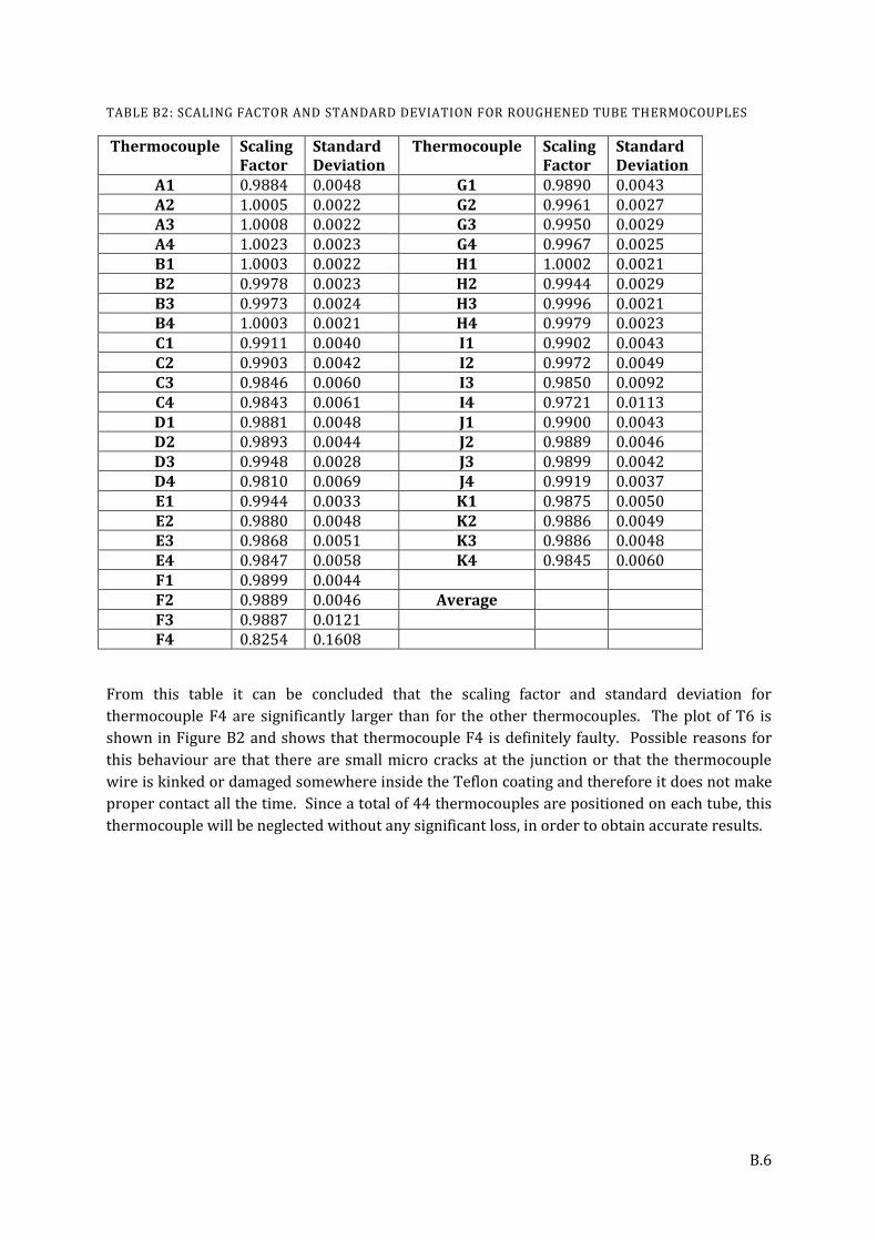
B.6
TABLE B2: SCALING FACTOR AND STANDARD DEVIATION FOR ROUGHENED TUBE THERMOCOUPLES
Thermocouple Scaling Factor
Standard Deviation
Thermocouple Scaling Factor
Standard Deviation
A1 0.9884 0.0048 G1 0.9890 0.0043 A2 1.0005 0.0022 G2 0.9961 0.0027 A3 1.0008 0.0022 G3 0.9950 0.0029 A4 1.0023 0.0023 G4 0.9967 0.0025 B1 1.0003 0.0022 H1 1.0002 0.0021 B2 0.9978 0.0023 H2 0.9944 0.0029 B3 0.9973 0.0024 H3 0.9996 0.0021 B4 1.0003 0.0021 H4 0.9979 0.0023 C1 0.9911 0.0040 I1 0.9902 0.0043 C2 0.9903 0.0042 I2 0.9972 0.0049 C3 0.9846 0.0060 I3 0.9850 0.0092 C4 0.9843 0.0061 I4 0.9721 0.0113 D1 0.9881 0.0048 J1 0.9900 0.0043 D2 0.9893 0.0044 J2 0.9889 0.0046 D3 0.9948 0.0028 J3 0.9899 0.0042 D4 0.9810 0.0069 J4 0.9919 0.0037 E1 0.9944 0.0033 K1 0.9875 0.0050 E2 0.9880 0.0048 K2 0.9886 0.0049 E3 0.9868 0.0051 K3 0.9886 0.0048 E4 0.9847 0.0058 K4 0.9845 0.0060 F1 0.9899 0.0044 F2 0.9889 0.0046 Average F3 0.9887 0.0121 F4 0.8254 0.1608
From this table it can be concluded that the scaling factor and standard deviation for
thermocouple F4 are significantly larger than for the other thermocouples. The plot of T6 is
shown in Figure B2 and shows that thermocouple F4 is definitely faulty. Possible reasons for
this behaviour are that there are small micro cracks at the junction or that the thermocouple
wire is kinked or damaged somewhere inside the Teflon coating and therefore it does not make
proper contact all the time. Since a total of 44 thermocouples are positioned on each tube, this
thermocouple will be neglected without any significant loss, in order to obtain accurate results.
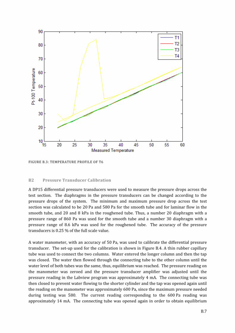
B.7
FIGURE B.3: TEMPERATURE PROFILE OF T6
B2 Pressure Transducer Calibration
A DP15 differential pressure transducers were used to measure the pressure drops across the
test section. The diaphragms in the pressure transducers can be changed according to the
pressure drops of the system. The minimum and maximum pressure drop across the test
section was calculated to be 20 Pa and 580 Pa for the smooth tube and for laminar flow in the
smooth tube, and 20 and 8 kPa in the roughened tube. Thus, a number 20 diaphragm with a
pressure range of 860 Pa was used for the smooth tube and a number 30 diaphragm with a
pressure range of 8.6 kPa was used for the roughened tube. The accuracy of the pressure
transducers is 0.25 % of the full scale value.
A water manometer, with an accuracy of 50 Pa, was used to calibrate the differential pressure
transducer. The set-up used for the calibration is shown in Figure B.4. A thin rubber capillary
tube was used to connect the two columns. Water entered the longer column and then the tap
was closed. The water then flowed through the connecting tube to the other column until the
water level of both tubes was the same, thus, equilibrium was reached. The pressure reading on
the manometer was zeroed and the pressure transducer amplifier was adjusted until the
pressure reading in the Labview program was approximately 4 mA. The connecting tube was
then closed to prevent water flowing to the shorter cylinder and the tap was opened again until
the reading on the manometer was approximately 600 Pa, since the maximum pressure needed
during testing was 580. The current reading corresponding to the 600 Pa reading was
approximately 14 mA. The connecting tube was opened again in order to obtain equilibrium

B.8
conditions in the two cylinders. The process was repeated three times in order to reduce the
effect of hysteris and the final current reading in the Labview program, corresponding to a
maximum pressure of 600 Pa was 13.16 mA.
The current signal obtained from the Labview program was converted to a pressure reading in
Excell. This was done via interpolation since the pressure ranged between 0 and 600 Pa and the
current between 4 and 13.16 mA . A plot of the pressure recorded by the Labview program
against the actual pressure reading on the manometer was then generated and is shown in
Figure B.5. The equation of the line was determined and used to determine the pressure drop
during the tests. However, after each start-up of the pumps, the pressure taps and pressure
transducer were bled to ensure that there is no air in the system. A pressure reading was then
taken during no-flow conditions and was used as the off-set. The no-flow condition was
obtained by opening the by-pass valve and closing the supply-valve in order to ensure that there
is water supply for the pump, but not through the test section. One reading consisting of
approximately 30 data points was taken and the average pressure reading was used as the off-
set value. The final pressure equation used in the Matlab code was therefore
.
FIGURE B.4: PRESSURE TRANSCDUCER CALIBRATION

B.9
FIGURE B.5: PRESSURE TRANSDUCER 1 CALIBRATION
This process was repeated for the second diaphragm and the following plot was generated:
FIGURE B.6: PRESSURE TRANSDUCER 2 CALIBRATION

C.1
APPENDIX C: MATLAB CODES
Appendix C contains the Matlab codes that were used to process the calibration and
experimental data. The codes for the smooth and roughened tubes are similar, therefore the
adiabatic friction factor code and 8.66 kW/m2 heat flux code for the roughened tube will be
included only.

D.1
APPENDIX D: PROTOCOL AND PROGRESS REPORTS
Appendix D contains the Protocol and Progress Reports which was used to inform the project
leader about the developments of the project.

D.2
UNIVERSITY OF PRETORIA
MSC 412 - PROTOCOL The Influence of Surface Roughness in the
Transitional Flow Regime
Marilize Everts S29037078
3/9/2012
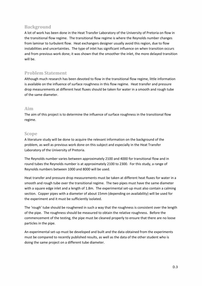
D.3
Background A lot of work has been done in the Heat Transfer Laboratory of the University of Pretoria on flow in
the transitional flow regime. The transitional flow regime is where the Reynolds number changes
from laminar to turbulent flow. Heat exchangers designer usually avoid this region, due to flow
instabilities and uncertainties. The type of inlet has significant influence on when transition occurs
and from previous work done; it was shown that the smoother the inlet, the more delayed transition
will be.
Problem Statement Although much research has been devoted to flow in the transitional flow regime, little information
is available on the influence of surface roughness in this flow regime. Heat transfer and pressure
drop measurements at different heat fluxes should be taken for water in a smooth and rough tube
of the same diameter.
Aim The aim of this project is to determine the influence of surface roughness in the transitional flow
regime.
Scope A literature study will be done to acquire the relevant information on the background of the
problem, as well as previous work done on this subject and especially in the Heat Transfer
Laboratory of the University of Pretoria.
The Reynolds number varies between approximately 2100 and 4000 for transitional flow and in
round tubes the Reynolds number is at approximately 2100 to 2300. For this study, a range of
Reynolds numbers between 1000 and 8000 will be used.
Heat transfer and pressure drop measurements must be taken at different heat fluxes for water in a
smooth and rough tube over the transitional regime. The two pipes must have the same diameter
with a square edge inlet and a length of 1.8m. The experimental set-up must also contain a calming
section. Copper pipes with a diameter of about 15mm (depending on availability) will be used for
the experiment and it must be sufficiently isolated.
The ‘rough’ tube should be roughened in such a way that the roughness is consistent over the length
of the pipe. The roughness should be measured to obtain the relative roughness. Before the
commencement of the testing, the pipe must be cleaned properly to ensure that there are no loose
particles in the pipe.
An experimental set-up must be developed and built and the data obtained from the experiments
must be compared to recently published results, as well as the data of the other student who is
doing the same project on a different tube diameter.

D.4
Method
The following method will be used to determine the influence of surface roughness in the
transitional flow regime:
Protocol
Literature study
Theoretical Simulation
Experimental set-up
Experiments
Correlations
Compare, discuss and process data
Compile Final Report
Prepare Presentation and oral
Poster exhibition
Deliverables Research Report
An experimental set-up to test the influence of surface roughness in the transitional flow
regime.
An oral presentation and poster exhibition
Target Dates Protocol 9 March 2012
First Progress Report 30 March 2012
Half year Report 28 May 2012
Half year evaluation 22 June 2012
Second Progress Report 27 August 2012
Closure of workshops 6 October 2012
Final Report 22 October 2012
Final Presentation and oral 16 November 2012
Poster Exhibition 29 November 2012
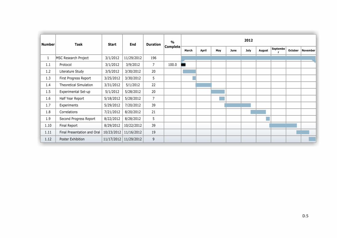
D.5

B.6
UNIVERSITY OF PRETORIA
INFLUENCE OF SURFACE ROUGHNESS IN THE
TRANSITIONAL FLOW REGIME
MSC – FIRST PROGRESS REPORT
Study Leader: Prof JP Meyer
Marilize Everts S29037078
3/30/2012
Prof J.P. Meyer
Marilize Everts

B.7
Work completed up to date Since there are mainly two groups of people who investigated the transitional flow regime, a
literature study has been done on the work done by Meyer and Ghajar. Diabatic and adiabatic
cases, as well as enhanced tubes were investigated.
Project Plan Since the required background knowledge needed for the project has been obtained, the theoretical
simulation process can be started before the actual experimental set-up can be designed. The
relevant information concerning the available laboratory equipment must be obtained, since this is
needed for the calculations. Options to roughen the inside of the tube must also be investigated in
order to select the best one.
Personal Opinion Up to now, no serious problems are foreseen except to find a suitable method to roughen the inside
of the tube uniformly. The project is still on schedule and if this schedule is further adhered to, all
the deadlines will be met and influence of the surface roughness in the transitional flow regime will
be determined.

B.8

D.9
UNIVERSITY OF PRETORIA
INFLUENCE OF SURFACE ROUGHNESS IN THE
TRANSITIONAL FLOW REGIME
MSC – SECOND PROGRESS REPORT
Study Leader: Prof JP Meyer
Marilize Everts
Marilize Everts
Prof J.P. Meyer
D.10
Status of work completed up to date The experimental set-up is almost done and the thermocouples have been calibrated and attached
to the two tubes. The second tube was roughened by a process similar to knurling. A steel bar was
roughened on the outside and inserted into the copper tube. A kinetic hammer was used to
hammer the copper tube and imprint the roughness on the inside. Metlab reported that the
roughness of the tube could not be measured since the needle got stuck in the grooves of the rough
surface and that the surface profile of the tube falls outside the capabilities of their roughness
tester. The maximum capability of their equipment is a surface roughness of 16 µm and when
dividing this with the inner tube diameter of 14.46 mm, a relative roughness of 0.001 was obtained.
This roughness was sufficient since the corresponding friction factors on the Moody Chart varied
between 0.044 and 0.035 for Reynolds numbers between 3 000 and 7 000, which is acceptable.
Project Plan The experimental set-up wil be completed within the next two week and afterwards the tests will be
conducted. During these last two weeks of the experimental set-up, Matlab codes will also be
written. Once the results are obtained, it can be inserted into the existing codes. These codes will
assist in investigating the friction factors and pressure drop and compare the two tubes with each
other.
Budget The experimental set-up is almost finished; therefore the majority of the costs is already made. The
rest of the costs are expected to be minimal. A summary of the total costs is given in the table
below. The material costs include everything that have been bought in order to build the
experimental set-up and to roughen the tube. The testing costs refer to the testing of the surface
roughness which was done by Metlab in order to determine the relative roughness of the tube.
Description Cost
Material 984.42
Testing 769.5
Total 1753.92
Personal Opinion Roughening the one tube was far more difficult and time consuming than initially expected, but
since the experimental set-up is nearly completed and the testing will soon commence, the project
will be completed on time.
The Gantt chart has been altered since there was not enough time allocated for building the
experimental set-up, and too much time was allocated for testing. The rest of the Gantt Chart is
similar to the previous one.

11