The influence of irradiance concentration using anasymmetric reflector on the electrical performance of

a PVT hybrid collector with standardmonocrystalline cells

Joel Nicolas Martınez Lopez

Thesis to obtain the Master of Science Degree in

Energy Engineering and Management

Supervisors: Prof. Luıs Filipe Moreira Mendes

Eng. Joao Santos Leite Cima Gomes

Examination Committee

Chairperson: Prof. Duarte de Mesquita e Sousa

Supervisor: Prof. Luıs Filipe Moreira Mendes

Member of the committee: Prof. Carlos Alberto Ferreira Fernandes

December 2016

ii

Dedicated to my parents

iii

iv

Acknowledgements

I would like to thank my thesis supervisor Dr. Luıs Filipe Moreira Mendes for his continuous support

during the work done in this thesis. His guidance and comments helped me at all time, driving my thesis

in the right direction.

My sincere thanks to Joao Santos Leite Cima Gomes for the opportunity to collaborate with Solarus and

for his support during the literature review stage. He was available any time that was needed to clarify

some data and technical issues.

I would also like to express my gratitude to KIC InnoEnergy for the funding received during my MSc.

studies. I acknowledge the contribution of CONACYT from Mexican Government for the financial sup-

port in my last semester.

Last but not the least, I must express my gratitude to my family and to my girlfriend for encouraging

me throughout these two years. This accomplishment would not have been possible without them.

v

vi

Resumo

O objetivo desta tese foi o de estudar o efeito da nao homogeneidade da irradiancia solar obtida pelo uso

de um concentrador assimetrico sobre o desempenho eletrico de um painel hıbrido fotovoltaico/termico

(CPVT). Para realizar trabalho foi implementado um acoplamento entre um software de raios tracadores

e dois modelos eletricos de um dıodo com tres e com cinco parametros, implementados em MATLAB. Os

modelos dividem as celula em pequenos elementos, que no caso do maior numero de divisoes tem uma

area de 0.65 mm2, considerando cada um deste elementos como uma unica celula solar. As simulacoes

foram realizadas alterando o numero e tamanho dos elementos, comparando-se os seus resultados com

os valores experimentais de um CPVT da empresa Solarus. A nao homogeneidade da irradiancia e o

uso termico do painel conduzem a uma temperatura tambem nao homogenea das celulas e a abordagem

utilizada foi o de atribuir algumas gamas de valores discretos a temperatura e analisar a sensibilidade

dos modelos a estes valores. Verificou-se que a nao homogeneidade da irradiancia afeta a curva I-V das

celulas, em particular o seu Fator de Preenchimento. No entanto esta diminuicao, para as condicoes

experimentais testadas, nao e superior a 1.3% em relacao a uma irradiancia homogenea.

Palavras-chave : irradiancia nao homogenea, coletor hıbrido fotovoltaico/termico, modelos eletricos de

celulas fotovoltaicas, desempenho de paineis fotovoltaicos.

vii

viii

Abstract

The objective of this thesis was to study the effect on a concentrating photovoltaic-thermal (CPVT)

collector caused by a non-homogeneous radiation, specifically on the electrical performance. In order to

accomplish the objective of this work, it was implemented a matching model using a raytrace software

and two electric models using the one diode model with 5 parameters and with 3 parameters. The model

divides the whole solar cell into small elements considering each of this elements as a unique solar cell,

which in the case of the higher number of divisions the small elements has an area of 0.65mm2. Some

simulations were carried out changing the number and size of the elements, comparing the results with the

experimental values obtained by a CPVT from the company Solarus. The solar cell will work at different

temperatures due to the non-homogeneous radiation, thus, the integration of a thermal model is necessary

and the approach employed was to test different discrete temperature levels and analyse the sensibility

of the models to the temperature. A non-homogeneous radiation affects the I-V curve, specifically the

fill factor, which is translated in a reduction of the maximum power. However, this decrease, for this

experimental tested conditions, does not exceed 1.3% in relation to an homogeneous irradiance.

Keywords: non-homogeneous radiation, hybrid PVT, electrical PV cells models, electrical PV perfor-

mance.

ix

x

Contents

Acknowledgements v

Resumo vii

Abstract ix

List of Figures xiii

List of Tables xv

Nomenclature xvii

Acronyms xix

1 Introduction 1

2 Literature review 3

2.1 Raytrace Software . . . . . . . . . . . . . . . . . . . . . . . . . . . . . . . . . . . . . . . . 3

2.1.1 TracePro . . . . . . . . . . . . . . . . . . . . . . . . . . . . . . . . . . . . . . . . . 3

2.1.2 OptiCAD . . . . . . . . . . . . . . . . . . . . . . . . . . . . . . . . . . . . . . . . . 4

2.1.3 SolTrace . . . . . . . . . . . . . . . . . . . . . . . . . . . . . . . . . . . . . . . . . . 5

2.1.4 Tonatiuh . . . . . . . . . . . . . . . . . . . . . . . . . . . . . . . . . . . . . . . . . 5

2.1.5 Shape and Material . . . . . . . . . . . . . . . . . . . . . . . . . . . . . . . . . . . 6

2.1.6 Sun shape and position . . . . . . . . . . . . . . . . . . . . . . . . . . . . . . . . . 7

2.2 Electrical Models . . . . . . . . . . . . . . . . . . . . . . . . . . . . . . . . . . . . . . . . . 8

2.2.1 Newton Raphson Method . . . . . . . . . . . . . . . . . . . . . . . . . . . . . . . . 10

2.2.2 Temperature and Radiation dependency . . . . . . . . . . . . . . . . . . . . . . . . 11

2.2.3 Non-homogeneous radiation . . . . . . . . . . . . . . . . . . . . . . . . . . . . . . . 12

2.2.4 Performance . . . . . . . . . . . . . . . . . . . . . . . . . . . . . . . . . . . . . . . 15

2.3 Solarus Collector . . . . . . . . . . . . . . . . . . . . . . . . . . . . . . . . . . . . . . . . . 17

3 Model 19

3.1 Modelling the Solarus collector in Tonatiuh . . . . . . . . . . . . . . . . . . . . . . . . . . 19

3.2 Electrical Model . . . . . . . . . . . . . . . . . . . . . . . . . . . . . . . . . . . . . . . . . 21

4 Results 25

4.1 Flux map comparison between Tonatiuh and Matlab . . . . . . . . . . . . . . . . . . . . . 25

4.2 Comparison between 5 and 3 parameters model . . . . . . . . . . . . . . . . . . . . . . . . 27

4.3 Temperature influence simulation with 148 x 1520 elements . . . . . . . . . . . . . . . . . 28

4.4 Homogeneous case - Simulation with 1 x 38 elements . . . . . . . . . . . . . . . . . . . . . 30

xi

4.5 Simulation with 5 x 38, 10 x 38 and 20 x 380 elements . . . . . . . . . . . . . . . . . . . . 31

4.6 Comparison between number of elements . . . . . . . . . . . . . . . . . . . . . . . . . . . . 35

5 Conclusions & Future Work 37

Bibliography 39

Appendix A Translate binary files into Matlab 43

Appendix B One diode 3 parameters for an element 47

Appendix C One diode 5 parameters for an element 49

Appendix D Temperature Dependency function 51

Appendix E Radiation Dependency function 53

Appendix F Current function 55

Appendix G Obtaining the current from .05V to .5V 57

Appendix H Obtaining maximum points 59

Appendix I Obtaining the open circuit voltage 63

Appendix J Comparison between flux map of Tonatiuh and Matlab 65

xii

List of Figures

1.1 CPC collector configuration . . . . . . . . . . . . . . . . . . . . . . . . . . . . . . . . . . . 1

1.2 Involute reflector . . . . . . . . . . . . . . . . . . . . . . . . . . . . . . . . . . . . . . . . . 1

2.1 TracePro simulation . . . . . . . . . . . . . . . . . . . . . . . . . . . . . . . . . . . . . . . 4

2.2 OptiCAD simulation . . . . . . . . . . . . . . . . . . . . . . . . . . . . . . . . . . . . . . . 4

2.3 Relative error of Tonatiuh . . . . . . . . . . . . . . . . . . . . . . . . . . . . . . . . . . . . 5

2.4 Pillbox shape used in Tonatiuh . . . . . . . . . . . . . . . . . . . . . . . . . . . . . . . . . 7

2.5 One diode equivalent circuit . . . . . . . . . . . . . . . . . . . . . . . . . . . . . . . . . . . 8

2.6 Ideal one diode equivalent circuit . . . . . . . . . . . . . . . . . . . . . . . . . . . . . . . . 9

2.7 Two diode equivalent circuit . . . . . . . . . . . . . . . . . . . . . . . . . . . . . . . . . . . 9

2.8 Heizer’s two dimensional equivalent circuit . . . . . . . . . . . . . . . . . . . . . . . . . . . 12

2.9 Mitchell’s two dimensional model . . . . . . . . . . . . . . . . . . . . . . . . . . . . . . . . 13

2.10 Mitchell’s one-dimensional model . . . . . . . . . . . . . . . . . . . . . . . . . . . . . . . . 13

2.11 Chenlo’s equivalent circuit arrangement . . . . . . . . . . . . . . . . . . . . . . . . . . . . 13

2.12 Quarter finger space unit . . . . . . . . . . . . . . . . . . . . . . . . . . . . . . . . . . . . 14

2.13 Franklin’s one dimensional equivalent circuit . . . . . . . . . . . . . . . . . . . . . . . . . . 14

2.14 Fill Factor . . . . . . . . . . . . . . . . . . . . . . . . . . . . . . . . . . . . . . . . . . . . . 15

2.15 Franklin’s I-V curves . . . . . . . . . . . . . . . . . . . . . . . . . . . . . . . . . . . . . . . 16

2.16 Herrero’s I-V curves . . . . . . . . . . . . . . . . . . . . . . . . . . . . . . . . . . . . . . . 16

2.17 Solarus CPVT collector . . . . . . . . . . . . . . . . . . . . . . . . . . . . . . . . . . . . . 17

2.18 Solarus MaReCo design . . . . . . . . . . . . . . . . . . . . . . . . . . . . . . . . . . . . . 17

2.19 Solarus absorber design . . . . . . . . . . . . . . . . . . . . . . . . . . . . . . . . . . . . . 17

2.20 One string arrangement . . . . . . . . . . . . . . . . . . . . . . . . . . . . . . . . . . . . . 18

3.1 Final geometry using Tonatiuh . . . . . . . . . . . . . . . . . . . . . . . . . . . . . . . . . 20

3.2 Rays reaching the collector . . . . . . . . . . . . . . . . . . . . . . . . . . . . . . . . . . . 20

3.3 Flux distribution on the PV arrangement . . . . . . . . . . . . . . . . . . . . . . . . . . . 21

3.4 Elevation of the sun . . . . . . . . . . . . . . . . . . . . . . . . . . . . . . . . . . . . . . . 21

3.5 Cell divided in small elements . . . . . . . . . . . . . . . . . . . . . . . . . . . . . . . . . . 22

3.6 Equivalent circuit of a cell . . . . . . . . . . . . . . . . . . . . . . . . . . . . . . . . . . . . 22

4.1 Comparison between flux map obtained by Tonatiuh and Matlab at 30(10 x 40 elements) 26

4.2 I-V curves using 5 and 3 parameters model . . . . . . . . . . . . . . . . . . . . . . . . . . 27

4.3 Radiation map with 148 x 1520 elements . . . . . . . . . . . . . . . . . . . . . . . . . . . . 28

4.4 I-V curves for 148 x 1520 elements . . . . . . . . . . . . . . . . . . . . . . . . . . . . . . . 28

4.5 Radiation map with 1 x 38 elements . . . . . . . . . . . . . . . . . . . . . . . . . . . . . . 30

4.6 Radiation map with 5 x 38 elements . . . . . . . . . . . . . . . . . . . . . . . . . . . . . . 31

4.7 Radiation map with 10 x 38 elements . . . . . . . . . . . . . . . . . . . . . . . . . . . . . . 31

xiii

4.8 Radiation map with 20 x 380 elements . . . . . . . . . . . . . . . . . . . . . . . . . . . . . 32

4.9 I-V curves for 5 x 38 elements . . . . . . . . . . . . . . . . . . . . . . . . . . . . . . . . . . 32

4.10 I-V curves for 10 x 38 elements . . . . . . . . . . . . . . . . . . . . . . . . . . . . . . . . . 33

4.11 I-V curves for 20 x 380 elements . . . . . . . . . . . . . . . . . . . . . . . . . . . . . . . . 33

xiv

List of Tables

2.1 Comparison between raytrace software . . . . . . . . . . . . . . . . . . . . . . . . . . . . . 6

2.2 Physical characteristics of Big Sun solar cell . . . . . . . . . . . . . . . . . . . . . . . . . . 18

2.3 Electrical properties of Big Sun solar cell . . . . . . . . . . . . . . . . . . . . . . . . . . . . 18

2.4 Typical Temperature Coefficients of Big Sun solar cell . . . . . . . . . . . . . . . . . . . . 18

2.5 Electrical Measures by Solarus . . . . . . . . . . . . . . . . . . . . . . . . . . . . . . . . . 18

2.6 Conditions of Solarus test . . . . . . . . . . . . . . . . . . . . . . . . . . . . . . . . . . . . 18

3.1 Parameters of the reflector used in Tonatiuh . . . . . . . . . . . . . . . . . . . . . . . . . . 20

3.2 Simulations done with the electrical model . . . . . . . . . . . . . . . . . . . . . . . . . . . 24

3.3 Temperatures used for “Hot” and “Cold” (2 zones) . . . . . . . . . . . . . . . . . . . . . . 24

3.4 Temperatures for different radiation ranges (5 zones) . . . . . . . . . . . . . . . . . . . . . 24

4.1 Power reaching the receiver at different elevation angles. . . . . . . . . . . . . . . . . . . . 25

4.2 Percentage difference between one diode with 5 parameters, 3 parameters and Solarus

simulation with respect to the measured values . . . . . . . . . . . . . . . . . . . . . . . . 27

4.3 String arrangement using 148 x 1520 elements . . . . . . . . . . . . . . . . . . . . . . . . . 29

4.4 Comparison between 2 and 5 “hot” and “cold” zones . . . . . . . . . . . . . . . . . . . . . 29

4.5 Comparison between non-homogeneous and homogeneous radiation at T = 40.5 . . . . . . 30

4.6 String arrangement using 5 x 38 elements . . . . . . . . . . . . . . . . . . . . . . . . . . . 34

4.7 String arrangement using 10 x 38 elements . . . . . . . . . . . . . . . . . . . . . . . . . . . 34

4.8 String arrangement using 20 x 380 elements . . . . . . . . . . . . . . . . . . . . . . . . . . 34

4.9 Comparison between number of elements . . . . . . . . . . . . . . . . . . . . . . . . . . . . 35

4.10 Percentage difference of number of elements with respect to the measured values . . . . . 35

xv

xvi

Nomenclature

Roman symbols

Aelement Area of an element [mm2].

A156 Area of the whole size cell [mm2].

Eg Band gap of the semiconductor [eV].

FF Fill factor.

Gre f Reference radiation (1000 W/m2).

G Radiation reaching the cell [W/m2].

ID Diode current [A].

IL Light current, also called photovoltaic current Iph [A].

Imax Maximum power point current [A].

Io Reverse diode saturation current [A].

Is Saturation current [µm].

Isc Short circuit current [A].

Ish Shunt current [A].

Ns Number of solar cells.

Pmax Maximum power [W].

Rs Series resistance [Ω].

Rsh Shunt resistance, also called parallel resistance (Rp) [Ω].

Vmax Maximum power point voltage [V].

Voc Open circuit voltage [V].

VT Thermal voltage [V].

VT,re f Thermal voltage at STC [V].

k Boltzman constant (1.381 × 10−23 J/K).

m Diode’s ideality factor.

q Modulus of electronic charge of cells in series (1.602 × 10−19 C).

Greek symbols

xvii

α Current temperature coefficient [mA/K].

β Voltage temperature coefficient [mV/K].

γ Ideality factor defined by Hejri et al. (2016).

xviii

Acronyms

CAD Computer Aided Design

CPC Compound Parabolic Concentrator

CPVT Compound Photovoltaic and Thermal

csr Circumsolar ratio

GUI Graphical user interface

MaReCo Maximum Reflector Concentration

PV Photovoltaic

STC Standard test conditions

xix

xx

Chapter 1

Introduction

The objective of this thesis is to determine how the non-homogeneous radiation affects the electrical

performance of a collector, particularly, in a Compound Photovoltaic and Thermal (CPVT) collector.

The work in this thesis was done in collaboration with Solarus Sunpower B.V. This is a private company,

founded in 2006. Solarus has its headquarters in the Netherlands with a R&D centre in Sweden. The

collector that is subject of study in this thesis is a CPVT collector designed and tested in Sweden. The

characteristics and properties of this collector are shown in the next chapter. This thesis aims to provide

the company with a better knowledge about its collector while general conclusions can be extracted from

the thesis work.

Solarus CPVT collector is very similar to the standard Compound Parabolic Concentrator (CPC) col-

lectors, it has a concentrator and a receiver. Then, a brief description of CPC collectors is presented.

The CPC collector consists of arrays of evacuated tubes with cylindrical absorbers with a back reflector

to direct radiation into the absorbers as seen on Figure 1.1. The reflectors are two parabolas around the

absorber which are intended to reflect all rays into the absorber. O’Gallagher et al. (1980) determined

that using an involute reflector will lead to the maximum energy captured by the absorbers, see Figure

1.2.

Figure 1.1: CPC collector configuration

(Duffie et al., 2013)

Figure 1.2: Involute reflector

(O’Gallagher et al., 1980)

It is necessary to measure the distribution of energy that can be concentrated by a collector. In this

sense, the use of raytrace software will help to cover this topic. It is difficult to obtain experimental data

on the distribution of the irradiance on the solar cells. Therefore, the use of a model can be an useful

analysis tool which results can be compared with experimental data to validate it.

The electrical model in this thesis is very important because with it, is possible to achieve the objective

proposed. Then, a previous objective to the main goal is to generate a proper model to simulate the

1

collector behaviour, forecasting the power, current and voltage for a given condition.

As a summary, the raytrace software was used to simulate the rays reaching the Solarus collector. The

rays are reflected by the special shape of the collector and reach the PV cells. The number and distribu-

tion of the photons were translated to Matlab for post-processing. An electrical code was generated in

Matlab and together with the photons distribution, the final model was created.

This thesis is organized in 5 chapters and appendices. Chapter 2 shows the different available raytrace

software and presents a comparison between them. It is also presented a literature review of the electrical

models to simulate a solar cell. The properties and geometry of the Solarus collector are shown as

well. Chapter 3 explains the methodology used, a deeper understanding of the selected raytrace software

and the electrical model approach used in this thesis. In Chapter 4 there are presented the results of

comparing the flux map in Tonatiuh vs Matlab. It is shown the results of comparing the one diode model

using 5 and 3 parameters. Also, the results from the simulation and comparison with different number

of elements are shown. Chapter 5 presents the conclusions of this thesis and future work that could be

done. The last part of this thesis is assigned to the appendices which includes all the Matlab codes and

functions developed in the master thesis.

2

Chapter 2

Literature review

This chapter is divided in three sections. Section 2.1 describes and compare the available raytrace software

that could be used in this thesis. In Section 2.2 it is presented the two main electrical circuits that model

a solar cell, including a method to solve the related equations. It also presents a literature review on

how to model a non-homogeneous radiation over a solar cell covering the possible parameters that could

be affected by the radiation and presents the parameters that measures the performance of a cell. This

section includes a review on the variables that affect the performance of a solar cell stated by other

authors. Lastly, Section 2.3 describes the Solarus collector: geometry and physical properties of the

reflector and support body. In the same way, it is described the physical properties of the absorber (solar

cells).

2.1 Raytrace Software

This section describes different raytrace software, namely TracePro, OptiCAD, SolTrace and Tonatiuh.

Their advantages, characteristics and capabilities are shown and compared. Tonatiuh was used to simulate

the rays reaching the collector, therefore, a deeper description of it is presented.

2.1.1 TracePro

TracePro is a commercial user friendly software used for design, analysis, and optimization of optical

and illumination systems (Lambda, 2016). The study object can be created using its own solid geometry

tools such as tubes, blocks, cones, spheres or by importing a CAD file. It also has the capability to model

optical elements such as lenses, reflectors and Fresnel lenses.

In its library, TracePro has many materials and surfaces properties that can be applied to an object or

surface. The properties that can be modified include index of refraction, absorption coefficient, reflectance

and transmittance coefficients, surface absorption, surface scatter, and fluorescence among others. In fact,

this software is very complete and has the specific features to model a system with high accuracy.

The main feature that is important in this study is the fast and accurate ability of TracePro’s ray tracing.

The main features declared by its creators are: ray splitting, exact ray tracing, an analysis mode ray

tracing for interactive viewing, and little or no memory consumption for large number of rays simulated.

A powerful tool included in TracePro is it analysis mode. It can show irradiance and radiance maps,

luminance maps, 3D irradiance maps displaying true color plots of the incident, absorbed, or exiting

3

flux onto the selected surfaces. TracePro includes polarization maps and volume flux maps. Its analysis

results can be filtered to show only the rays of a given wavelength or flux range. Of course, all its results

can be exported to a text file or a bitmap file. An example of TracePro is shown in Figure 2.1. The price

of Trace Pro is not available in its website, however, they state they have a free trial version of 30 days.

Figure 2.1: TracePro simulation

Lambda (2016)

2.1.2 OptiCAD

OptiCAD is an optical analysis software used for raytracing mainly: reflection, refraction, surface and

bulk scattering surface and bulk luminance, and polarization (OptiCAD Corp., 2016). With this soft-

ware many optical elements could be simulated such as: spherical and cylindrical lenses; flat, parabolic,

spherical or conical mirrors; CPC and Fresnel lenses; or any other CAD object. This software is capable

to model the light source as points, lines, surfaces, volumes, bitmaps, equations, or data tables. It can

also simulate multiple light sources in any location.

It has many functions and options to model any optical component. Its results could be shown in a

tabular form, directly in 3D form. It has the ability to show energy and intensity maps, irradiance and il-

luminance maps, 3D ray tracing among others. Its advantages over others come with a price, the product

and 1 year license cost 3500 USD (OptiCAD Corp., 2016). After downloading and running the demo, it

was observed that even though its a graphical user interface (GUI), it is not as easy-to-use as Tonatiuh.

Figure 2.2 shows an example on how OptiCAD shows some rays over a surface and an intensity map.

Figure 2.2: OptiCAD simulationOptiCAD Corp. (2016)

4

2.1.3 SolTrace

SolTrace is a software tool developed by the National Renewable Energy Laboratory. The objective of

this software is to simulate and analyze a concentrated solar power (CSP) system. It is used mainly

in solar applications, but it can also be used in any other optical system. SolTrace uses Monte Carlo

ray trace method. The number of rays can be selected to run in the simulation, more rays means a

better accuracy, nevertheless, the processing time also increases. SolTrace uses C++ code that is fast

and compatible with any computer. However, not everybody is comfortable with text coding and a user

friendly interface should be used. SolTrace uses the helping tool SketchUp which is free and easy to

use and with it a better user interaction is on hand. The results obtained by SolTrace can be seen as

scatter plots and flux maps. Moreover, a set of data can be saved and then used with other software for

post-processing. An interesting feature is the scripting tool incorporated in SolTrace, with it the user

can perform parametric simulations.

2.1.4 Tonatiuh

Tonatiuh is raytrace software used in solar concentrating systems that simulates optical properties and

shapes (Blanco, 2016). This software is open source, this means, anyone can use it or modify it. It is

simple, accurate and easy to use.

In the same way as SolTrace, Tonatiuh is based on Monte Carlo method to generate rays. Taking into

account the random foundation of Monte Carlo method, it is important to set a high number of rays

generated in order to have a good simulation.

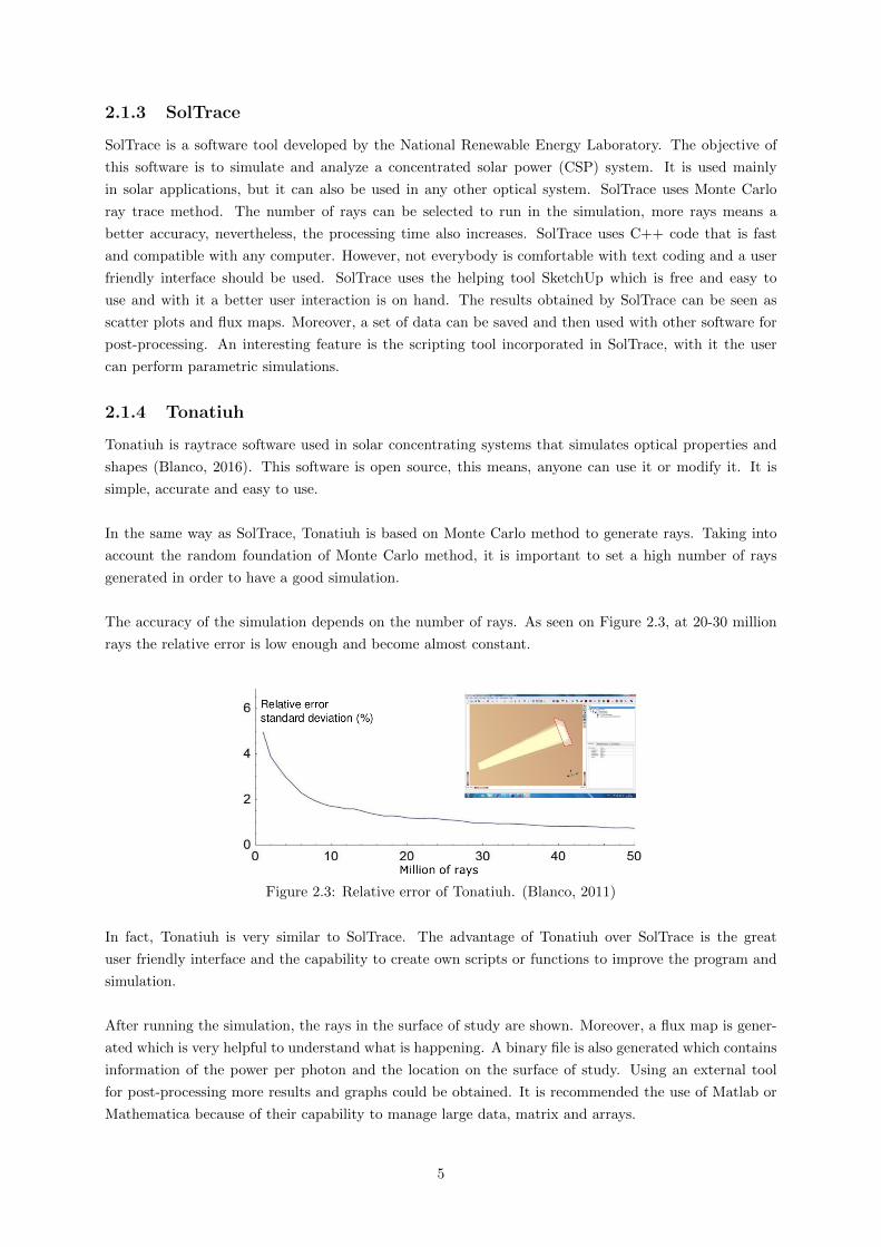
The accuracy of the simulation depends on the number of rays. As seen on Figure 2.3, at 20-30 million

rays the relative error is low enough and become almost constant.

Figure 2.3: Relative error of Tonatiuh. (Blanco, 2011)

In fact, Tonatiuh is very similar to SolTrace. The advantage of Tonatiuh over SolTrace is the great

user friendly interface and the capability to create own scripts or functions to improve the program and

simulation.

After running the simulation, the rays in the surface of study are shown. Moreover, a flux map is gener-

ated which is very helpful to understand what is happening. A binary file is also generated which contains

information of the power per photon and the location on the surface of study. Using an external tool

for post-processing more results and graphs could be obtained. It is recommended the use of Matlab or

Mathematica because of their capability to manage large data, matrix and arrays.

5

Tonatiuh was selected as the software to be used in the master thesis because of its easy use, same results

compared to SolTrace and because it is free. The differences, between Tonatiuh and SolTrace, in power

are so small that are negligible, and the differences of maximum flux density are also negligible when the

number of photons is one million or more (Blanco et al., 2009).

Table 2.1 shows a comparison between the four available software packages, where it is demonstrated

the advantage of Tonatiuh over others: user friendly, easy to add own scripts and geometries, exportable

data capability and free of charge.

Table 2.1: Comparison between raytrace software

InterfaceDesign

PricePost-

processingMaterialLibraries

TracePro Excellent N/AOwn analysis

featureExcellent

Opticad Good 3500 USDOwn analysis

featureN/A

SolTraceCould beimproved

Free uponregistration

Exportable data N/A

Tonatiuh Excellent Free Exportable data Poor

It was already discussed the reason of using Tonatiuh in this work. Next subsections describe two

important parameters when using Tonatiuh: shape & material, and solar shape. The shape refers to the

geometry of study, which can have different reflection index and other factors that are modified under

the material tab, as shown in the next paragraphs. The other important parameter is the solar shape

that is the way Tonatiuh will simulate the rays.

2.1.5 Shape and Material

Under the shape section different geometries can be chosen, enumerating the most used: flat rectangle,

parabolic dish, sphere, through CPC, through parabola among others. There is another option, released

in the last version 2.2.0, which enables to insert a CAD solid.

A material can be selected for each shape. Tonatiuh incorporates several options for materials, the most

used are: basic refractive material and specular standard material. Mirrors and absorber surfaces use

specular standard material differing one from the other in the reflectivity property, where a reflectivity

of 1 corresponds to a perfect mirror and 0 to the absorber.

The mirror quality, optical losses in general (surface imperfections, structure deformations, etc.) and

slope-error are integrated in the sigma-slope property. Tonatiuh sets a value of 2 (typical value) for

default, a value of 0 will model an ideal material with no losses and an increase value will lead to a higher

error, meaning, the rays will reflect in other ways than desired. If there is no enough information, the

typical value of 2 can be selected.

The solar shape error is taken into account under the distribution property which is set under the define

sunlight option and will be discussed in the next section.

The last parameters of the specular standard material are ambient color, diffuse color, specular color,

emissive color, shininess and transparency. Each of them only account on the way the solid material will

be shown on Tonatiuh and are not considered for calculations.

6

2.1.6 Sun shape and position

The sun shape is the radial distribution of energy considering the sun as a non-punctual source of light.

Tonatiuh includes two different sun shapes: Buie and Pillbox.

Buie model takes into account the energy from the solar disk and from the circumsolar aureole. A very

detailed description of this model is shown in Buie et al. (2003). It is important to notice that Buie shape

is a more realistic model since takes into account both, solar disk and circumsolar aureole.

Pillbox shape is simpler. It considers the solar disk as a constant source of light, with constant radiance

over a cone of directions from the center of the Sun of a given half-angle and drops to zero at higher

angles, which means that its angular distribution is constant.

For both sun shapes, it is necessary to define the solar irradiance in W/m2. For the Buie shape, one must

be set the circumsolar ratio (csr) which is the energy coming from the circumsolar region expressed as

percentage of the total energy coming from the sun. In the Pillbox shape the other parameter to define

is the angle theta max, Tonatiuh predefine this solar disk angle as 4.65 mrad. This means the solar

intensity is the same in every point of the sun, as seen on Figure 2.4.

The position of the sun is established by its azimuth and elevation. The azimuth is the distance in

degrees, between the north and the location of the sun. For example, east will be 90, south 180, and west

270. Usually, solar devices (solar cells, thermal, CPC, etc.) are mounted facing south. The altitude is

also measured in degrees being 90 normal to the horizontal.

Tonatiuh has the option to calculate the solar position by means of the location in the Earth and at a

certain day, called Sun Position Calculator. This tool is very helpful to simulate radiation everywhere is

necessary.

Figure 2.4: Pillbox shape used in Tonatiuh

7

2.2 Electrical Models

The behavior of a solar cell under radiation and temperature different from the standard test conditions

(STC) can be predicted using an electric model. All models use information from manufacturers namely

Imax , Vmax , Isc and Voc. The idea is to obtain the current-voltage (I-V) characteristic of a solar PV and

then use this data to work on the maximum power point.

The modeling of a solar cell has been studied from decades. Nowadays, the one diode model and the two

diode model are the most used when modeling a PV cell, each model includes several parameters.

The equivalent circuit of a solar cell using one diode is presented in Figure 2.5. Duffie et al. (2013)

determined the I-V characteristic where they use 5 parameters described by Equation 2.1

I = IL − ID − Ish = Il − Io

[exp

(V + IRs

m′VT

)− 1

]− V + IRs

Rsh(2.1)

Where:

IL = Light current, also called photovoltaic current (Iph).

Io = Reverse diode saturation current.

Rs = Series resistance.

Rsh = Shunt resistance, also called parallel resistance (Rp).

VT = Thermal voltage.

m′ = Diode’s ideality factor.

The thermal voltage is directly proportional to the cell temperature and it is related to some physical

constants, it is given by Equation 2.2

VT =kTq

(2.2)

Where:

k = Boltzman constant (1.381 × 10−23J/K).

T = Cell temperature.

q = Modulus of the electronic charge of cells in series (1.602 × 10−19C).

Ideality factor m′ is the factor for a whole solar panel. It is the result of multiplying the ideality factor

of a single cell, m, times the number of cells in the solar panel, as shown on Equation 2.3

m′ = mNs (2.3)

The ideality factor for a single cell is equal to 1 for an ideal diode and typically between 1 and 2 for real

diodes.

Figure 2.5: One diode equivalent circuit

There is also a one diode model which uses 3 parameters and does not take into account the series and

shunt resistance as seen on Equations 2.4 to 2.6 (Markvart and Castaner, 2003). This approach considers

8

the solar cell as ideal solar cell with no losses. Therefore, is not as accurate as the one diode model with

5 parameters but may result in much less computing effort and time. Its equivalent circuit is shown in

Figure 2.6.

m =Vmax − Voc

VT log(1 − Imax

Isc

) (2.4)

Io =Isc

exp(Voc

mVT

) − 1 (2.5)

Is = Isc (2.6)

Figure 2.6: Ideal one diode equivalent circuit

The two diode model is similar to the one diode, but incorporates a second diode in parallel as seen

on Figure 2.7. The two diode model increases its accuracy at lower irradiance (Alrahim Shannan et al.,

2013). It is clear that the two diode model has more variables and is more complex. The I-V characteristic

for the two diode model is given by Equation 2.7

I = IL − Io1

[exp

(V + IRs

m′1VT1

)− 1

]− Io2

[exp

(V + IRs

m′2VT2

)− 1

]− V + IRs

Rsh(2.7)

Where:

Io1= Reverse saturation currents of diode 1.

Io2= Reverse saturation currents of diode 2.

VT1= Thermal voltage of diode 1.

VT2= Thermal voltage of diode 2.

m′1= Diode 1 ideality factor.

m′2= Diode 2 ideality factor.

Figure 2.7: Two diode equivalent circuit

Humada et al. (2016) presents a compilation of different methods to extract the parameters of the one

diode and two diode models. Methods and models use five, four, three, two and one parameters. In his

study, it was proven that the one diode model is very effective for simulating PV modules with converters

and that two diode models will lead to better results if the module is working under normal conditions,

namely STC. Elbaset et al. (2015) and Gow and Manning (1999) present a two diode model in function

of temperature and solar radiation. Since the I-V characteristic curve is non-linear they used the Newton

9

Raphson method to solve the multivariable system of equations derived in their model.

It has been demonstrated that using the 1 diode model is an accurate and a low complex model (Humada

et al., 2016). Most models use the manufacturer information and need some extra data that should be

obtained from experiments. As stated by Hejri et al. (2016) it is possible to use a set of equations with

only manufacturer’s data. This proposal doesn’t need to evaluate the solar cell experimentally, making

the calculations and modeling a fast and easier way than other models.

Hejri et al. (2016) equations, 2.8, 2.9 and 2.10, are relevant for this study and are shown below for

reference. He got three equations with three unknown variables Rs, Rsh and γ. They called γ to the

ideality factor. These equations, as any other one diode model, has to be solved by a numerical method

namely Newton-Raphson.

Imax

Vmax− 1

γVT

(1 − Rs

Imax

Vmax

) (−Voc + (Rs + Rsh)Isc

Rsh

)exp

(Vmax − Voc + Rs Imax

γVT

)− 1

Rsh

(1 − Rs

Imax

Vmax

)= 0

(2.8)

−Imax

(1 +

Rs

Rsh

)+

(−Voc + (Rs + Rsh)Isc

Rsh

) [1 − exp

(Vmax − Voc + Rs Imax

γVT

)]+

Voc − Vmax

Rsh= 0

(2.9)

− Rs

Rsh+

Rsh − Rs

γVT+

(−Voc + (Rs + Rsh)Isc

Rsh

)exp

(Rs Isc − Voc

γVT

)= 0 (2.10)

However, using Newton-Raphson must ensure to have a good initial guess. Hejri et al. (2016) arrived at

a set of equations, 2.11, 2.12 and 2.13, that give good initial values for Rs, Rsh and γ:

γ =2Vmax − Voc

VT[ln

(Isc−Imax

Isc

)+

Imax

Isc−Imaxa

] (2.11)

Rs =Vmax

Imax−

2Vmax−Voc

Isc−Imax

ln(Isc−Imax

Isc

)+

Imax

Isc−Imax

(2.12)

Rsh =

√√√ Rs

IscγVT

exp(Rs Isc−Voc

γVT

) (2.13)

Using Newton-Raphson to solve Hejri equations it is possible to get the solar cell parameters and obtain

its I-V curve.

2.2.1 Newton Raphson Method

This is a method for root finding, which is used for finding solutions of a system of non-linear equations.

Newton-Raphson method uses one initial guess x0 and uses Taylor series to obtain a new value.

10

f (x) = f (x0) + f ′(x0)(x − x0) +1

2f ′′(x0)(x − x0)2 + · · · = 0 (2.14)

Where x is the real root and x0 the initial guess. When the initial guess is close to the real root, x − x0will be small and the first terms of the Taylor series will be the important ones, leading to a simplification

of the Newton-Raphson method:

xi+1 = xi −f (xi)f ′(xi)

(2.15)

Starting with an initial guess, a new value will be obtained. The original equation is evaluated with the

new value and checked if it satisfies it, if not, the procedure is repeated using the new value as initial

guess until convergence is obtained.

For a multivariable set of equations it is used the partial derivative of each variable with respect each of

the other variables, this is in mathematics called the Jacobian as seen below:

J =∂( f1, f2, . . . , fn)∂(x1, x2, . . . , x3)

=

©­­­­­­­­«

∂( f1)∂(x1)

∂( f1)∂(x2) · · ·

∂( f1)∂(xn)

∂( f2)∂(x1)

∂( f2)∂(x2) · · ·

∂( f2)∂(xn)

......

. . ....

∂( fn)∂(x1)

∂( fn)∂(x2) · · ·

∂( fn)∂(xn)

ª®®®®®®®®¬(2.16)

Using the Jacobian, Newton Raphson method will be:

xi+1 = xi − J−1 f (2.17)

In order to solve this type of equations is necessary the use of a powerful software such as Matlab.

2.2.2 Temperature and Radiation dependency

The VT and Io parameters from the one diode model depend on temperature; Isc and Rsh depend on irradi-

ance; and Is and Voc depend on both temperature and irradiance. Using Equations 2.18 to 2.21 (de Jesus,

2015; Luque and Hegedus, 2011) is possible to obtain new parameters that depend on temperature.

VT = VT,re fT

Tre f; (2.18)

Io = Io,re f

(T

Tre f

)3exp

[qm

(Eg,re f

kTre f−

Eg

kT

)](2.19)

Is = Is,re f + α(T − Tre f ); (2.20)

Voc = Voc,re f + β(T − Tre f ); (2.21)

Where α and β are the thermal coefficients of current and voltage respectively.

Equations 2.22 to 2.25 (de Jesus, 2015; Luque and Hegedus, 2011) are used to obtain parameters that

depend on irradiance.

Isc = Gnew

Isc,re fGre f

(2.22)

Rsh = Gre f

Rsh,re f

Gnew(2.23)

11

Is = Gnew

Is,re fGre f

(2.24)

Voc = mVT log

[(IsRsh) − Voc

Rsh Io

](2.25)

2.2.3 Non-homogeneous radiation

The most common procedure to study a cell under non-uniform radiation is to divide the cell in subcells

which will act as a one diode model or two diode model (Baig et al., 2012). Each of the elements is

connected in series or parallel depending in the model selected. Models proposed by some authors in-

clude two dimensional current flow, this means that current generated by a single element could travel

horizontally or vertically adding its current to the next element until reach a finger and finally the busbar.

Heizer and Chu (1976) present an equivalent circuit of a solar cell in a two dimensional matrix as shown

on Figure 2.8. Current generated by the cell could be conducted in x or y direction.

Figure 2.8: Two dimensional equivalent circuit.(Heizer and Chu, 1976)

Mitchell (1977) presented a two-dimensional matrix model in order to evaluate the effects of non-uniform

illumination on the solar cell. It is stated that the homogeneous radiation influences the efficiency through

modifying the resistance losses in the solar cell. Figure 2.9 shows the equivalent circuit for a single ele-

ment of the two-dimensional model and the paths of the current flow. Notice the similarity to Heizer and

Chu (1976) proposal. In addition to the model proposal, a comparison between it and a one-dimensional

model is performed. The one-dimensional model equivalent circuit is presented in Figure 2.10. This

model only takes into account a current flow in the x direction, this is, a group of one diode model cells

are connected in parallel adding their currents. The author also incorporates a small top layer resistance

of 5 ohms per square which will lead to minimize the effects of non-homogeneous illumination. It is also

stated that the top layer resistance might be obtained using transparent electrode materials.

12

Figure 2.9: Two dimensional model. (Mitchell, 1977)

Figure 2.10: One-dimensional model. (Mitchell, 1977)

Chenlo and Cid (1987) present a thermal and electric model when solar cells receive non uniform illumi-

nation. As other authors, they divide the cell in subcells. It is considered a one dimensional current flux

and simulated using the equivalent circuit shown in Figure 2.11. Subcells are connected in parallel and

the sum of each column is added to the next one, this means that current generated is the addition of all

subcells.

Figure 2.11: Equivalent circuit arrangement. (Chenlo and Cid, 1987)

This study also demonstrates that cell efficiency is reduced when the cell temperature rises and when a

non-uniform radiation occurs. Authors noticed that if studying temperature and non-uniform radiation

at the same time, the impacts will be more intense than taking temperature and non-uniformity sepa-

rately and adding their effects.

Franklin and Coventry (2002) compared the effects of a homogeneous illumination against a non-uniform

illumination. Solar cells working under non-homogeneous illumination have a decrease in open circuit

voltage and efficiency compared to a uniform case even though both cases receive the same amount of

radiation. Authors divide the solar cell in identical elements that consist of a quarter finger space unit

13

as seen on Figure 2.12, similarly as many authors. Initially it was considered a two dimensional current

flow, however it was simplified to a one dimensional problem using the approximation that the current

flow is normal to the finger. The equivalent circuit for each unit is shown on Figure 2.13.

Figure 2.12: Quarter finger space unit.(Franklin and Coventry, 2002)

Figure 2.13: One dimensional equivalent circuit. (Franklin and Coventry,2002)

14

2.2.4 Performance

Using the electric model it is possible to predict the efficiency of the solar cell without a real testing

allowing to modify any distribution, connections, arrangement, cell properties, etc. and have a result im-

mediately. The two characteristic to rate the performance of a solar cell and/or module are its efficiency

and Fill Factor(FF) (Duffie et al., 2013). Since it is mandatory to keep the solar cell working at the

maximum power point the efficiency and FF are measured using maximum power points. The efficiency

is given by eq 2.26

θ =Pmax

A G(2.26)

Where:

Pmax= Maximum power.

A= Area that gathers the radiation.

G= Irradiance reaching the cell.

The Fill Factor corresponds to the ratio between a theoretical power and the real maximum power, a

ratio between areas of two rectangles as shown on Figure 2.14. The rectangle defined by Isc and Voc is

the theoretical power and the Imax and Vmax rectangle is the maximum power. FF will always be less

than 1. A more squared FF is preferable. The FF is given by eq 2.27

FF =Pmax

Voc Isc(2.27)

Where:

Pmax= Maximum power.

Voc= Open circuit voltage.

Isc= Short circuit current.

Figure 2.14: Fill Factor

Both Efficiency and FF, among others, are affected due to non-uniform radiation as stated by sev-

eral authors. Luque et al. (1998) demonstrated that a non-homogeneous illumination will increase the

temperature and series resistance, reducing the PV efficiency. Furthermore, under a non-homogeneous

illumination the fill factor, efficiency, and open circuit voltage decrease (Mellor et al., 2009).

15

It was demonstrated that the performance of a solar cell depends on the spectral intensity distribution

(Schultz et al., 2012). A better uniform distribution will extend lifetime and increase performance of

the cell and module. In the same way, Reis et al. (2015) proved the importance of using distributed

models when simulating solar cells under non-homogeneous temperature and radiation. At non-uniform

illumination, simulating a cell as a lumped model will overestimate its resistive losses and thus, will lead

to an insufficient simulation.

Since non-homogeneous radiation increases the temperature and thus a reduction in the PV efficiency

(Luque et al., 1998) a good option is to incorporate a thermal system to maintain an optimal temperature.

Proell et al. (2016) studied a PVT hybrid collector and concluded that in a compound parabolic con-

centrator (CPC) reflector, the PV efficiency is negative influenced by the temperature and illumination

distribution as well as optical losses due to mirrors and ohmic losses due to solar concentration.

Figure 2.15 shows how the maximum current and voltage drops when cells are under non uniform illu-

mination and temperature (Franklin and Coventry, 2002), this means the fill factor will decrease. The

same result was obtained by Herrero et al. (2012) as shown on Figure 2.16. Having a uniform distribution

increase the efficiency of the cell.

Figure 2.15: I-V curves

(Franklin and Coventry, 2002)

Figure 2.16: I-V curves

(Herrero et al., 2012)

16

2.3 Solarus Collector

The Solarus collector is a CPVT device of 2374 x 1027 x 231 mm as seen on Figure 2.17. The collector

could be divided in four parts, the holding base, the protective glass, the reflector, and the absorber.

The holding base is made of plastic and holds everything in place. The protective glass is 4 mm thick

and has an anti reflective coating. This glass is made of low iron glass and has a transmittance of 0.9

at normal incidence angle (Bernardo et al., 2013). It is known that refraction for a low iron glass is

1.52 (ABRISA Technologies, 2010). The reflector uses a Maximum Reflector Concentration (MaReCo)

technology designed by Solarus which consists of an asymmetrical parabolic through, maximizing as much

as possible the concentrated energy into the absorber. Figure 2.18 illustrates the reflector. The reflector

material is made of anodised aluminium with a solar reflection of approximately 90% (Bernardo et al.,

2013). The absorber could be divided into three parts, the lower and upper PV arrangements and the

thermal exchanger. The thermal exchanger are tubes where water flows while it is heated. These tubes

are between the lower and upper PV arrangements, just like a sandwich as seen on Figure 2.19.

Figure 2.17: Solarus CPVT collector

(Solarus Sunpower B.V., 2015)

Figure 2.18: Solarus MaReCo design

(Solarus Sunpower B.V., 2015)

Figure 2.19: Solarus absorber design

(Solarus Sunpower B.V., 2015)

Both, lower and upper, arrangements consist of two strings connected in parallel where one string is

composed by 38 solar cells. Each solar cell is monocrystalline with a length of 26 mm and width of 148

mm. Then, one string measures 988 mm x 148 mm as seen on Figure 2.20.

The monocrystalline cells are from Big Sun with physical characteristics shown in Table 2.2 and electrical

properties shown in Table 2.3. The temperature coefficients of this solar cell are also important and are

shown in Table 2.4, notice that the current coefficient is called α and the voltage coefficient β. This cells

are squared of 156 mm x 156 mm, thus, they must be cut to have 148 mm in one side and then must be

17

divided in 6 to have the desired dimension of 148 mm x 26 mm. Solarus apply this arrangement in order

to reduce the amount of current produced by the cells.

Figure 2.20: One string arrangement

Table 2.2: Physical characteristics of Big Sun solar cell. (SunPower, 2015)

Dimension 156 mm x 156 mm x ±0.5 mm

Diagonal 200 mm ±1.0 mm

Thickness 200 µm ±30 µm

Front Three silver busbars, anisotropically texturized surface with dark

blue silicon nitride anti-reflection coating

Back Full-surface aluminium BSF, Silver / Aluminium soldering pads

Table 2.3: Electrical properties ofBig Sun solar cell. (SunPower, 2015)

Efficiency (%) 19.4

Pmax (W) 4.634

Vmax (V) 0.537

Imax (A) 8.631

Voc (V) 0.639

Isc (A) 9.158

Table 2.4: Typical Temperature Coefficients ofBig Sun solar cell. (SunPower, 2015)

α +5.16 mA/K

β -1.2 mV/K

Solarus provided some test results of the behaviour of two strings connected in parallel. In the next

chapter, these results will act as reference values and will be compared with those obtained by an own

model. The results and conditions of Solarus test are shown in Table 2.5 and 2.6

Table 2.5: Electrical Measures by Solarus

Pmax(W) 47.3

Imax(A) 2.7

Isc(A) 3.1

Voc(V) 22

Vmax(V) 17.51

FF(%) 68.7

Electrical

efficiency (%)17.6

Table 2.6: Conditions of Solarus test

Tin (C) 39.3

Tout (C) 41.8

Flow (l/min) 2.22

Tamb(V) 21.9

Panel Orientation Facing sun

Panel Tilt () 30

Solar Irradiation

(W/m2)921

Date of measurements 04/Aug/2015 11:05

18

Chapter 3

Model

This chapter contains the procedures that were followed to simulate the Solarus collector. It is divided

in 2 sections. The first section contains information about the selected raytrace software, Tonatiuh. The

objective of using a raytrace software is to predict the amount of energy that will reach the absorber.

Here, it is explained how the Solarus collector was modelled and how the simulation was carried out.

After getting the amount of energy reaching the absorber, it is necessary to predict the amount of power

to be generated by the collector. The second section presents the electrical model to forecast the power

generated.

3.1 Modelling the Solarus collector in Tonatiuh

The Solarus collector consists of a reflector and a receiver. The reflector has a parabolic and a cylindrical

part (asymmetric through). The receiver element has PV cells at the upper and lower side, while in the

middle it has tubes for the heat transfer. This geometry was translated into Tonatiuh coupling basic

geometries such as cylinders, parabolic solids and rectangles. Tonatiuh is capable of showing the amount

and distribution of the rays reaching a desired area. This data is then exported to a binary file for

post-processing.

The cylindrical part of the reflector has a radius of 144.51 mm. It is a quarter of a circle with length of 2327

mm. In order to create it in Tonatiuh it is necessary to define the angle φmax = 90 (1.570796327rad)

which will create a cylinder from 0to 90, a quarter of a circle. Notice that Tonatiuh uses radians

instead of degrees. Just after the cylindrical reflector there is an extension of it, which could be taken

as a rectangle sheet of 2327 mm long and 42.27 mm wide. The parabolic reflector has a focus length of

144.51 mm (same as the cylindrical radius). The length of it is 2327 mm. It is mandatory to establish

the distance from the origin to the final point of the parabola, this distance is 325 mm. Table 3.1 shows

the parameters introduced in Tonatiuh to obtain the desired geometry, Table 3.1a shows the dimensions

of the cylindrical part and Table 3.1b shows the dimensions of the parabolic part. The material of the

reflector is considered to have a reflectivity of 0.9 as mentioned in Section 2.3. The sigma slope error

(optical losses) is considered to be 2, the typical value as explained in Section 2.1.5.

19

Table 3.1: Parameters of the reflector used in Tonatiuh

(a) Cylindrical part

Radius 0.14451 m

Length 2.3269999 m

phiMax 1.5707964 rad

(b) Parabolic Part

Focus length 0.14451 m

xMin 0 m

xMax 0.32499999 m

LengthXMin 2.3269999 m

LengthXMax 2.3269999 m

The absorber could be taken as a rectangular box integrated by an upper and lower PV cells arrange-

ment. It is 157 mm wide, 2310 mm long and 14.5 mm tall. Inside it is a tube arrangement for the heat

transfer process. It is only necessary to define a rectangular solid in Tonatiuh, nevertheless, the location

is very important and need to be calculated with precision. This absorber is modelled to capture all rays

reaching it surface and not reflect any, thus, the reflectivity is set to 0.

This collector has a protective glass that preserves the solar cells and the mirror from the climatic con-

ditions. It is low iron glass with a transmittance of 0.9 and a refraction of 1.52 as explained in Section 2.3.

The environment in Tonatiuh was set to match the conditions of the day when Solarus ran its test. It was

selected a Pillbox sunshape in order to have the same solar intensity in every point of the sun and it was

defined to have an irradiance of 921 W/m2. The location of the sun was established using Tonatiuh’s sun

position calculator, requiring only the date input. The collector was facing south with a tilt of 30, this

was accomplished by generating rotation axis in Tonatiuh. Figure 3.1 shows the final geometry output

in different views, while Figure 3.2 shows how the rays reaching the collector (notice that the number of

rays displayed in this figure are for illustrative purposes only).

Figure 3.1: Final geometry using Tonatiuh

Figure 3.2: Rays reaching the collector

20

The raytrace test was simulated using 20 million rays since at this number the relative error decrease

as seen on Section 2.1.4. The surface of study was the lower PV arrangement of one string, this is, the

surface of 38 cells where the concentrating rays approach. Then, a binary file was generated exporting

all photon map coordinates. This file will be used for post-processing in Matlab. With Tonatiuh it was

possible to obtain a flux map of the string as seen on Figure 3.3.

Figure 3.3: Flux distribution on the PV arrangement

Moreover, a simulation using different elevation angles of the sun was done while the collector faces up

(without any tilt), in order to compare it with the simulations on Matlab and verify that the code from

Matlab is working correctly. The elevation of the sun will vary every 10 starting at 10 as shown on

Figure 3.4. The flux distribution and total power received by the collector will be compared.

Figure 3.4: Elevation of the sun

3.2 Electrical Model

This section explains the procedure of the creation of the electrical model and its implementation on

Matlab. The complete code, model and functions developed in this thesis are located under the Appen-

dices.

First of all, it is necessary to translate the binary files from Tonatiuh in order to have the distribution

of the photons and be able to work with the data (see Appendix A). Knowing the amount of photons,

location and their energy it was successfully determined the local radiation per each finite element. Then

the electrical model can be applied. There are two methods to evaluate the non-uniformity radiation

on solar cells. One is to use a finite element method, but the most common is to divide the cell into

sub-circuits described by the one diode or two diode model as seen on Section 2.2.3. The approach to

study the effect of a non-homogeneous radiation was adapted from Proell et al. (2016) where the cell is

divided in finite elements and each element is modelled as a one single cell. Each element will produce

21

its own current, different from the other elements since the radiation reaching each subcell is different.

The solar cell could be divided as many elements as necessary. Some assumptions to take in consideration

are: No current transfer between rows and, radiation on a single element is homogeneous. Figure 3.5

shows a part of a cell divided in small elements. As stated previously, the current generated by an element

is added to the next one until it reaches the finger and then it flows into the busbar, the red arrows show

how the current flows. Each element is modelled using the one diode model with 5 parameters since it

is more accurate than the 3 parameters model. The numerical proposal from Hejri et al. (2016) will be

used to obtain the 5 parameters of the single diode model. The equivalent circuit of the cell using the

single diode model is shown on Figure 3.6. This approach will lead to have tiny elements of 0.65 mm x 1

mm, for the 38 cells, a total of 224,960 elements need to be simulated. Even though the use of Matlab (or

other software) will reduce processing time, the iterative solution for the equations will take an enormous

time to be processed. Since every cell has the same properties and as observed by Tonatiuh’s flux map,

it was decided to model only one of the cells and then scaled the results to the whole string.

Figure 3.5: Cell divided in small elements Figure 3.6: Equivalent circuit of a cell

The small elements will have the same electrical properties between them but different to the original

solar cell because they have a different area. When cutting a solar cell, its Vmax and Voc remain constant.

In the other hand, the current and temperature coefficients are proportional to the area. Equations 3.1

to 3.4 were used to obtain the new values of Isc, Imax and temperature coefficients for the small elements.

Isc,element = Isc,156Aelement

A156; (3.1)

Imax,element = Imax,156Aelement

A156; (3.2)

αelement = αAelement

A156; (3.3)

βelement = βAelement

A156; (3.4)

22

For each element (1 mm x 0.65 mm) Rs, Rsh, Is, Io and VT were computed, where all of them except Rs

depend on irradiance and will need to be evaluated with the irradiance obtained by Tonatiuh. In order

to obtain the values it is used the Hejri et al. (2016) equations and the Newton Raphson method to solve

them (see Appendix C).

Having all parameters it is possible to evaluate each element. However, some parameters depend on

radiation and/or temperature and still need to be defined. VT , Io depend on temperature and Isc, Rsh

depend on irradiance while Is, Voc depend on both temperature and irradiance. Equations from Section

2.2.2 were used to obtain the new values. The Matlab code for temperature and irradiance dependency

can be found on Appendix D and Appendix E respectively.

For every radiation reaching the cell, a different temperature will appear. It is important to highlight

that the temperature used in the simulation is an average of the whole cell and not a temperature for

each element. In order to have the temperature for every element its necessary to add a thermal model

which is not included in this thesis and is proposed as future work under Chapter 5.

The next step is to obtain the values of current generated by each element for a given voltage. In this

way, it is possible to get the I-V curve and the maximum points of the solar cell arrangement. For now,

since only one cell is being modelled, the current generated is assume to be the same in the 38 cells of a

string and since the cells are connected in series, the voltage will be multiplied by 38. Then, since there

are two strings connected in parallel, the current doubles. The code to obtain the current for a given

voltage can be found on Appendix F. The procedure is repeated for values of voltage from 0 V to .5 V

where it is found that no more current is generated as if the arrangement was in open circuit. For the

coding of this process see Appendix G.

With the values of current and voltage it is calculated the power generated and the maximum power

point is obtained. This step was done calculating the power for a given voltage and moving to the right

or left depending where the highest point was until reaching a maximum point. See Appendix H for

the code. The open circuit voltage was obtained giving values to the voltage and increasing it until the

current obtained was close to zero. This was repeated until having a voltage with 4 digits, for example

0.4987. See Appendix I for this code.

After this procedure, it is obtained the Pmax , Imax , Vmax , Isc, Voc of the two strings connected in paral-

lel, each string made of 38 cells dividing each cell in small elements of 0.65 mm x 1 mm as stated previously.

The same process is now done using the one diode model with 3 parameters and the results are compared.

The simulation using only 3 parameters is to observe and compare the results and computing time. The

code of the the 3 parameters model is shown in Appendix B. Notice that the difference between 5 and 3

parameters is the use of series and shunt resistances in the one diode with 5 parameters model.

A series of simulations were done using the one diode with 5 parameters model but now changing the

number and size of the elements. Table 3.2 shows the total of simulations done with their respective

number of elements and size. The objective of these simulations is to determine if the final results are

affected by changing size and number of elements.

Since it is difficult to implement a detailed thermal model, and thus, obtain the temperature for every

element, it was decided to use a much simple model that could observed the influence of establishing

23

different variations of temperature and different temperature discretization as stated below.

There are included more simulations but now specifying “hot” and “cold” zones in the cells. The “hot”

zone will be above average temperature and “cold” zone will be below. For example, if average temper-

ature is 40.5C and defining a ∆T = 5C, the “hot” zone will be 45.5C and the “cold” will be 35.5C.

In order to know which elements are on the “hot” or “cold” zone, it is established that elements with

radiation above 1500W/m2 will be at “hot” zone and elements below 1500W/m2 will be in the “cold”

zone. It was selected 1500W/m2 because it is at the middle of the range of radiation, however, any other

radiation could be selected. This experiment has as an objective to see how different temperatures in the

same solar cell could affect its behaviour. For the temperature variations done in these simulations see

Table 3.3. This simulation is repeated but now considering five zones instead of two. The temperature

range was set to be 35.5C to 45.5C divided in five sections as well as the radiation. Since data from

radiation is known, it is obtained the maximum and minimum radiation reaching the surface and divided

in five sections as well. Table 3.4 shows the defined temperature for every range of radiation. Please

notice that the simulation using five temperature zones was only done for the 148 x 1520 elements.

Table 3.2: Simulations done with the electrical model

SimulationHorizontal

divisions

Vertical

divisions

Number of

elements

Size of an

element

Area of an

element

1 148 1520 224,960 1 mm x 0.65 mm 0.65 mm2

2 1 38 38 26 mm x 148 mm 3848 mm2

3 5 38 190 26 mm x 29.6 mm 769.6 mm2

4 10 38 380 26 mm x 14.8 mm 384.8 mm2

5 20 380 7600 2.6 mm x 7.4 mm 19.24 mm2

Table 3.3: Temperatures used for “Hot” and “Cold” (2 zones)

Simulation ∆T(C)Hot zone

temperature (C)

Cold zone

temperature (C)

a 5 45.5 35.5

b 10 50.5 30.5

c 15 55.5 25.5

d 20 60.5 20.5

Table 3.4: Temperatures for different radiation ranges (5 zones)

Radiation ranges (W/m2) Temperature (C)

10102.8-12628.5 45.5

7577.1-10102.8 43

5151.4-7577.1 40.5

2525.7-5051.4 38

0-2525.7 35.5

24

Chapter 4

Results

This chapter is dedicated to present the results from all the simulations carried out. Section 4.1 shows

the results of comparing the flux map from Tonatiuh and the one obtained with the Matlab code to verify

that the coding is correct. Section 4.2 presents the comparison results between the one diode model with

5 parameters and with 3 parameters. Section 4.3 shows the temperature influence on the solar cell. In

Section 4.4 it is presented the results for the homogeneous simulation. Section 4.5 presents the results of

the simulations with different element size and using the “hot” and “cold” zones approach. It is presented

the radiation map, the I-V curves and the Pmax , Vmax , Imax , Isc and Voc values for every situation. Notice

that the simulations were done using the same day and location parameters used by Solarus when they

made their test in order to be able to compare the results.

4.1 Flux map comparison between Tonatiuh and Matlab

Before running any of the simulations it is necessary to check that the code when translating the binary

files into Matlab is working correctly. Table 4.1 shows the power at the receiver obtained by Tonatiuh

and by Matlab.

Table 4.1: Power reaching the receiver at different elevation angles.

Elevation angle

10 20 30 40 50 60 70 80 90

Tonatiuh 8.65984 55.5065 97.3757 128.726 153.855 191.667 224.89 246.103 101.682

Matlab 8.6841 55.5393 97.3952 128.8798 153.7022 191.6209 224.8791 246.2889 101.4984

Matlab code is calculating correctly the power reaching the receiver. The next step is to demonstrate

that the code of Matlab is reading the flux map correctly. At this point it is not necessary to show all the

figures, only the 30 is shown in Figure 4.1. However, all of the other figures can be seen on Appendix

J. After comparing the power and the radiation distribution, it is demonstrated that the Matlab code is

working correctly, and that the next simulations will use proper data.

Also, it is visible how the solarus collector can concentrate the energy of the sun at different angles (see

Appendix J).

25

Figure 4.1: Comparison between flux map obtained by Tonatiuh and Matlab at 30(10 x 40 elements)

26

4.2 Comparison between 5 and 3 parameters model

A simulation using the one diode model with 5 and 3 parameters was done. Figure 4.2 shows the I-V

curves for both simulations. It is observed that the one diode model with 3 parameters model have a

higher power and current, this is because it is not taken into account the losses in the series and shunt

resistances. Table 4.2 shows the percentage difference for the one diode model with 5 and 3 parameters

and Solarus estimation if we take as reference the measured values (Table 2.5). The one diode model

with 5 parameters has the closest values to the measured ones and thus, the smallest percentage difference.

The one diode model using 3 parameters is much more faster than using 5 parameters, i.e. a simula-

tion to obtain current points for 148 x 1520 elements last 494 seconds, this is around 8 minutes, while

a simulation using 5 parameters can last up to 21609 seconds, this is, 6 hours. The one diode with 5

parameters model incorporates the series and shunt resistances and takes much time because it needs to

solve simultaneous equations.

Figure 4.2: I-V curves using 5 and 3 parameters model

Table 4.2: Percentage difference between one diode with 5 parameters, 3 parameters and Solarus simula-tion with respect to the measured values

5 parameters 3 parameters Solarus simulation

Pmax (W) 0.8% 3.5% 77.0%

Imax (A) 16.1% 19.3% 39.6%

Isc(A) 14.3% 14.3% 28.1%

Voc (V) 15.7% 13.6% 11.7%

Vmax (V) 13.2% 13.2% 26.7%

27

4.3 Temperature influence simulation with 148 x 1520 elements

Figure 4.3 shows the flux map with 224960 elements obtained by Matlab code. Since the number of

elements is very high, it is possible to see with high accuracy the location where the concentration

occurs. Figure 4.4 shows the I-V curves with the average temperature, and with different variations of

“hot” and “cold” zones as explained in Section 3.2. Table 4.3 presents the Pmax , Vmax , Imax , Isc and

Voc for all cases. Table 4.4 presents the results for the simulation using five temperature zones and a

comparison between it and the two zones simulation.

Figure 4.3: Radiation map with 148 x 1520 elements

Figure 4.4: I-V curves for 148 x 1520 elements

28

Table 4.3: String arrangement using 148 x 1520 elements

T = 40.5 C ∆T = 5 C ∆T = 10 C ∆T = 15 C ∆T = 20 CMeasured

Values

Pmax (W) 47.6559 47.6153 47.1997 46.2559 44.7804 47.3

Imax (A) 3.1353 3.2975 3.1849 3.2033 3.0216 2.7

Isc (A) 3.5429 3.5330 3.5231 3.5132 3.5033 3.1

Voc (V) 18.5554 18.6808 18.7606 18.7910 18.7606 22

Vmax (V) 15.2000 14.4400 14.8200 14.4400 14.8200 17.51

Table 4.4: Comparison between 2 and 5 “hot” and “cold” zones

T = 40.5 C∆T = 5 C

(2 zones)

∆T = 5 C

(5 zones)

Pmax (W) 47.6559 47.6153 48.9782

Imax (A) 3.1353 3.2975 3.2223

Isc (A) 3.5429 3.5330 3.5354

Voc (V) 18.5554 18.6808 18.9316

Vmax (V) 15.2000 14.4400 15.2000

As seen on Figure 4.4 a higher variation of temperature will lead to a power reduction. This is because

the zone where most of radiation reaches is at a higher temperature than expected.

If we compare the results of Table 4.3 to the measured ones, it is seen that a variation in temperature of

15C and 20C will lead to a poor forecast of the power.

In Table 4.4, the five temperature zones approach forecast a higher power. The main observable reason

for this to happen is that for a certain radiation range, the temperature associated does not correspond

to it. Another reason, that could be happened at the same time, is that the temperature does not change

5C, but 10C.

29

4.4 Homogeneous case - Simulation with 1 x 38 elements

Figure 4.5 shows the flux map with 38 elements obtained by Matlab code. This simulation is considering

the size of one element equal to the size of the solar cell. As stated in Section 3.2, one of the assumptions

is that the radiation is homogeneous inside an element. Thus, this simulation could be considered as

homogeneous. Because of this, is not possible to have “hot” and “cold” zones and as consequence an I-V

curve is not shown. What it is possible is to show a comparison between a non-homogeneous simulation

(148 x 1520 elements) and the homogeneous simulation. Table 4.5 presents the Pmax , Vmax , Imax , Isc and

Voc for the non-homogeneous and homogeneous simulation.

Figure 4.5: Radiation map with 1 x 38 elements

Table 4.5: Comparison between non-homogeneous and homogeneous radiation at T = 40.5

Non-homogeneous Homogeneous

Pmax (W) 47.6559 47.9150

Imax (A) 3.1353 3.2331

Isc (A) 3.5429 3.4975

Voc (V) 18.5554 18.6010

Vmax (V) 15.2000 14.82

From Table 4.5, a non-homogeneous radiation will affect the maximum power, current and voltage. The

maximum voltage seems to increase under non-homogeneous radiation in 2.5%, however, the maximum

current is decreased in 3%. Short circuit current and open circuit voltage are not so affected by non-

homogeneous radiation. Short circuit current increase by 1.3% and open circuit voltage almost does not

change.

30

4.5 Simulation with 5 x 38, 10 x 38 and 20 x 380 elements

Figure 4.6, Figure 4.7 and Figure 4.8 shows the flux map with 190, 380 and 7600 elements respectively

obtained by Matlab code. Figure 4.9, Figure 4.10 and Figure 4.11 shows the I-V curves with the average

temperature and with different variations of “hot” and “cold” zones as explained in Section 3.2 for 190,

380 and 7600 elements respectively. Table 4.6, Table 4.7 and Table 4.8 presents the Pmax , Vmax , Imax , Iscand Voc for 190, 380 and 7600 elements respectively and for all cases.

It is observed, in Table 4.6, that the temperature affects the operation of the solar cell. The temperature

and power are indirectly proportional, while increasing the temperature, the power is being reduced. In

table 4.7 it is observed that when having an increase in the maximum temperature of 20C the cell does

not generate the same amount of current, and thus, a reduction of 5% if compared to the power measured.

Figure 4.6: Radiation map with 5 x 38 elements

Figure 4.7: Radiation map with 10 x 38 elements

31

Figure 4.8: Radiation map with 20 x 380 elements

Figure 4.9: I-V curves for 5 x 38 elements

32

Figure 4.10: I-V curves for 10 x 38 elements

Figure 4.11: I-V curves for 20 x 380 elements

33

Table 4.6: String arrangement using 5 x 38 elements

T = 40.5 C ∆T = 5 C ∆T = 10 C ∆T = 15 C ∆T = 20 CMeasured

Values

Pmax (W) 47.7512 47.2966 46.3918 45.1643 43.9070 47.3

Imax (A) 3.2221 3.1914 3.2127 3.2123 3.1228 2.7

Isc (A) 3.4974 3.4877 3.4779 3.4681 3.4584 3.1

Voc (V) 18.5744 18.5706 18.5098 18.3844 18.1830 22

Vmax (V) 14.8200 14.8200 14.4400 14.0600 14.0600 17.51

Table 4.7: String arrangement using 10 x 38 elements

T = 40.5 C ∆T = 5 C ∆T = 10 C ∆T = 15 C ∆T = 20 CMeasured

Values

Pmax (W) 47.6641 47.6692 47.0447 46.0514 44.8035 47.3

Imax (A) 3.2162 3.2165 3.1744 3.1892 3.1027 2.7

Isc (A) 3.4974 3.4877 3.4779 3.4681 3.4584 3.1

Voc (V) 18.5630 18.6580 18.6960 18.6770 18.5896 22

Vmax (V) 14.8200 14.8200 14.8200 14.4400 14.4400 17.51

Table 4.8: String arrangement using 20 x 380 elements

T = 40.5 C ∆T = 5 C ∆T = 10 C ∆T = 15 C ∆T = 20 CMeasured

Values

Pmax (W) 48.2544 48.0486 47.3872 46.2771 45.0973 47.3

Imax (A) 3.2560 3.2421 3.1975 3.1226 3.2075 2.7

Isc (A) 3.5429 3.5330 3.5231 3.5132 3.5033 3.1

Voc (V) 18.5744 18.6618 18.6998 18.6770 18.5896 22

Vmax (V) 14.8200 14.8200 14.8200 14.8200 14.0600 17.51

34

4.6 Comparison between number of elements

Table 4.9 shows a comparison between the five simulations using different size and thus, number, of

elements. The power obtained when simulating at 224,960 elements is very close to the reference values

measured by Solarus. It is demonstrated that increasing the number of elements will lead to a closer

value, of Pmax , Imax and Vmax , with low difference error as seen on Table 4.10.

Table 4.9: Comparison between number of elements

Number of elements

224,960 7600 380 190 38

Pmax (W) 47.6559 48.2544 47.6641 47.7512 47.9150

Imax (A) 3.1353 3.2560 3.2162 3.2221 3.2331

Isc (A) 3.5429 3.5429 3.4974 3.4974 3.4975

Voc (V) 18.5554 18.5744 18.5630 18.5744 18.6010

Vmax (V) 15.2000 14.8200 14.8200 14.8200 14.8200

Table 4.10: Percentage difference of number of elements with respect to the measured values

Number of elements

224,960 7600 380 190 38

Pmax (W) 0.8% 2.0% 0.8% 1.0% 1.3%

Imax (A) 16.1% 20.6% 19.1% 19.3% 19.7%

Isc(A) 14.3% 14.3% 12.8% 12.8% 12.8%

Voc (V) 15.7% 15.6% 15.6% 15.6% 15.5%

Vmax (V) 13.2% 15.4% 15.4% 15.4% 15.4%

35

36

Chapter 5

Conclusions & Future Work

The one diode model with 3 parameters is faster than the one diode model with 5 parameters. However,

using the 5 parameters model provides a more accurate result. The one diode model with 3 parameters

can be used only to know a fairly value of the power that can be obtained. It is recommended to be used

when an approximation of the power, voltage and current is needed. For a more precise forecast the one

diode with 5 parameters model is used.

When simulating at “hot” and “cold” zones, it was demonstrated that the maximum and minimum tem-

peratures of the cell is near the average point, ±10C but no more than ±15C where it was seen that

the power, current and voltage have a higher percentage difference.

The use of more than two “hot” and “cold” zones can be used. For the case of having a maximum and

minimum temperatures 5C higher and lower respectively, the five temperature zones approach forecast

a higher power. This is why it is really necessary to have a point where for a given radiation its temper-

ature is known, so it can be used as a reference and to be able to divide in proper regions. Moreover, the

maximum temperature of the cell could be higher than 5C above the average, this assumption implies

the use of other temperatures, i.e. 10C.

It is also demonstrated that having an homogeneous distribution of radiation, will lead to slightly im-

provement of the performance of the collector. Under non-homogeneous radiation Vmax increases while

Imax decreases, which lead to a lower power output. Voc also decreases as other authors suggest (see

Section 2.2.3)

An electrical model using 3 or 5 parameters was built and coded in Matlab. With the help of Tonatiuh, it

was possible to compute the distribution and energy of the photons reaching a surface. The simulations

and forecast are close to the reference measures and could be considered as a helpful model if one wants

to know the order of magnitude of the generated power.

As a final conclusion, it is observed that the radiation affects the parameters which are used to model

the collector, Isc, Rsh, Is and Voc, however, this impact is not as significant as the effect produced by the

temperature, which includes parameters such as, VT , Io, Is and Voc, but more important is the impact

on the I-V curve, fill factor and finally in the maximum power, voltage and current. A non-homogeneous

radiation affects negatively, and indirectly, the electrical performance of the collector. It is said indirectly

because the impact received by the parameters are almost insignificant. Nevertheless, a non-homogeneous

radiation will lead to a temperature distribution in the solar cell, which will cause a modification in the

37

performance of the solar cell.

As a proposed future work, the thermal module needs to be added to the current model. In order to have a

more accurate model, it is required to make the calculations of a single element using a temperature closer

to the real one. This implies that the thermal and electrical models need to be solved simultaneously.

Including the thermal model in the CPVT, it could be possible to forecast the final temperature of the

fluid that is being heated only knowing the inlet temperature and the radiation reaching the collector as

inputs.

38

Bibliography

ABRISA Technologies. ABRISA Technologies, 2010. URL http://abrisatechnologies.com/

products-services/glass-products/soda-lime-glass/low-iron/. [Accessed on: 17-09-2016].

N. M. A. Alrahim Shannan, N. Z. Yahaya, and B. Singh. Single-diode model and two-diode model

of PV modules : A comparison. In Control System, Computing and Engineering (ICCSCE), 2013

IEEE International Conference, pages 210–214. Mindeb, 2013. ISBN 9781479915088. doi: 10.1109/

ICCSCE.2013.6719960. URL http://ieeexplore.ieee.org/stamp/stamp.jsp?tp=&arnumber=

6719960&isnumber=6719916.

H. Baig, K. C. Heasman, and T. K. Mallick. Non-uniform illumination in concentrating solar cells.

Renewable and Sustainable Energy Reviews, 16(8):5890–5909, 2012. ISSN 13640321. doi: 10.1016/j.

rser.2012.06.020.

R. Bernardo, H. Davidsson, N. Gentile, C. Gruffman, L. Chea, and C. Mumba. Measurements of the

Electrical Incidence Angle Modifiers of an Asymmetrical Photovoltaic/Thermal Compound Parabolic

Concentrating-Collector. Engineering, 5(01):37, 2013. ISSN 1947-3931. doi: 10.4236/eng.2013.51b0.

M. J. Blanco. Status of Tonatiuh as of July 2011, 2011. URL http://www.slideshare.net/

manueljblanco/status-of-tonatiuh-as-of-july-2011. [Accessed on: 14-04-2016].

M. J. Blanco. Tonatiuh, 2016. URL http://iat-cener.github.io/tonatiuh/. [Accessed on: 14-04-

2016].

M. J. Blanco, A. Mutuberria, P. Garcia, R. Gastesi, and V. Martin. Preliminary validation of Tonatiuh.

In SolarPaces 2009 International Conference, Berlin, 2009. URL https://www.researchgate.net/

publication/212165994.

D. Buie, A. G. Monger, and C. J. Dey. Sunshape distributions for terrestrial solar simulations. Solar

Energy, 74(2):113–122, 2003. ISSN 0038092X. doi: 10.1016/S0038-092X(03)00125-7.

F. Chenlo and M. Cid. A linear concentrator photovoltaic module: analysis of non-uniform illumi-

nation and temperature effects on efficiency. Solar Cells, 20(1):27–39, feb 1987. ISSN 03796787.

doi: 10.1016/0379-6787(87)90018-4. URL http://www.sciencedirect.com/science/article/pii/

0379678787900184.

J. M. de Jesus. Lecture of PV Systems at Instituto Superior Tecnico. 2015.

J. A. Duffie, W. A. Beckman, and W. M. Worek. Solar Engineering of Thermal Processes. John Wiley

& Sons, Inc., Hoboken, New Jersey, 4 edition, 2013. ISBN 9781118418123. doi: 10.1115/1.2930068.

URL http://books.google.com/books?hl=en&lr=&id=qkaWBrOuAEgC&pgis=1.

39

A. A. Elbaset, H. Ali, and M. A. El Sattar. Deduction of two-diode model parameters for photovoltaic

system. In 3rd International Conference on Energy Systems and Technologies International Confer-

ence on Energy Systems and Technologies, pages 121–135, 2015. URL www.afaqscientific.com/

icest2015/Proc15/Abd-El_Sattar8.pdf.

E. T. Franklin and J. S. Coventry. Effects of highly non-uniform illumination distribution on electrical

performance of solar cells. In 40th Annual Conference for the Australian New Zealand Solar Energy

Society. ANU Research Publications, 2002. URL http://hdl.handle.net/1885/40832.

J. Gow and C. Manning. Development of a photovoltaic array model for use in power-electronics simula-

tion studies. IEE Proceedings - Electric Power Applications, 146(2):193–200, 1999. ISSN 13502352. doi:

10.1049/ip-epa:19990116. URL http://ieeexplore.ieee.org/stamp/stamp.jsp?tp=&arnumber=

766195&isnumber=16599.

K. Heizer and T. Chu. Solar cell conducting grid structure. Solid-State Electronics, 19(6):471–472,

1976. ISSN 00381101. doi: 10.1016/0038-1101(76)90009-5. URL http://www.sciencedirect.com/

science/article/pii/0038110176900095.

M. Hejri, H. Mokhtari, M. R. Azizian, and L. Soder. An analytical-numerical approach for parameter

determination of a five-parameter single-diode model of photovoltaic cells and modules. International

Journal of Sustainable Energy, 35(4):396–410, 2016. ISSN 1478-6451. doi: 10.1080/14786451.2013.

863886. URL http://dx.doi.org/10.1080/14786451.2013.863886.

R. Herrero, M. Victoria, C. Domınguez, S. Askins, I. Anton, and G. Sala. Concentration photo-

voltaic optical system irradiance distribution measurements and its effect on multi-junction solar cells.

PROGRESS IN PHOTOVOLTAICS: RESEARCH AND APPLICATIONS, 20(4):423–430, 2012. doi:

10.1002/pip.1145.

A. M. Humada, M. Hojabri, S. Mekhilef, and H. M. Hamada. Solar cell parameters extraction based on

single and double-diode models: A review. Renewable and Sustainable Energy Reviews, 56:494–509,

2016. ISSN 18790690. doi: 10.1016/j.rser.2015.11.051. URL http://dx.doi.org/10.1016/j.rser.

2015.11.051.

Lambda. TracePro, 2016. URL http://www.lambdares.com. [Accessed on: 14-04-2016].

A. Luque and S. Hegedus. Handbook of Photovoltaic Science and Engineering. Wiley, 2011. ISBN

9780470976128. URL https://books.google.es/books?id=sLMkCsde1u4C.

A. Luque, G. Sala, and J. Arboiro. Electric and thermal model for non-uniformly illuminated con-

centration cells. Solar Energy Materials and Solar Cells, 51(3-4):269–290, 1998. ISSN 09270248.

doi: 10.1016/S0927-0248(97)00228-6. URL http://www.sciencedirect.com/science/article/pii/

S0927024897002286.

T. Markvart and L. Castaner. Practical Handbook of Photovoltaics: Fundamentals and Applications.

Electronics & Electrical. Elsevier, 2003. ISBN 9781856173902. URL https://books.google.es/

books?id=gf6oN2Hl3RYC.

A. Mellor, J. Domenech-Garret, D. Chemisana, and J. Rosell. A two-dimensional finite element

model of front surface current flow in cells under non-uniform, concentrated illumination. So-

lar Energy, 83(9):1459–1465, 2009. ISSN 0038092X. doi: 10.1016/j.solener.2009.03.016. URL

http://www.sciencedirect.com/science/article/pii/S0038092X09000772.

40

K. W. Mitchell. Computer analysis of resistamce and non-uniform illumination effects on concentrator

solar cells. Electron Devices Meeting, 23:229–232, 1977. doi: 10.1109/IEDM.1977.189214. URL http:

//ieeexplore.ieee.org/stamp/stamp.jsp?tp=&arnumber=1479294&isnumber=31771.

J. J. O’Gallagher, A. Rabl, R. Winston, and W. McIntire. Absorption enhancement in solar collectors by

multiple reflections. Solar Energy, 24(3):323–326, 1980. ISSN 0038092X. doi: 10.1016/0038-092X(80)

90490-9.

OptiCAD Corp. OptiCAD, 2016. URL http://www.opticad.com/. [Accessed on: 14-04-2016].

M. Proell, H. Karrer, C. Brabec, and A. Hauer. The influence of CPC reflectors on the electrical

incidence angle modifier of c-Si cells in a PVT hybrid collector. Solar Energy, 126:220–230, 2016. ISSN

0038092X. doi: 10.1016/j.solener.2016.01.012. URL http://linkinghub.elsevier.com/retrieve/

pii/S0038092X16000256.

F. Reis, M. Pravettoni, J. Wemans, G. Sorasio, and M. C. Brito. Modelling the effects of inhomogeneous

irradiation and temperature profiles on CPV cells behaviour. IEEE Journal of Photovoltaics, 5(1):

112–122, 2015. ISSN 21563381. doi: 10.1109/JPHOTOV.2014.2358080. URL http://ieeexplore.

ieee.org/stamp/stamp.jsp?tp=&arnumber=6930715&isnumber=6991619.

R. D. Schultz, F. J. Vorster, and E. E. Van Dyk. Performance of multi-junction cells due to illumination

distribution across the cell surface. Physica B: Condensed Matter, 407(10):1649–1652, 2012. ISSN

09214526. doi: 10.1016/j.physb.2011.09.108. URL http://dx.doi.org/10.1016/j.physb.2011.09.

108.

Solarus Sunpower B.V. Solarus, 2015. URL http://solarus.com/our-solution/. [Accessed on: 19-

10-2016].

SunPower. A-300 Solar cell mono crystalline silicon. 2015. URL www.sunpowercorp.com. [Accessed on:

19-10-2016].

41

42

Appendix A

Translate binary files into Matlab

% Raytrace Function

function [radiation,Power_at_receiver,no_elements,avg] = raytrace_function(files,data)

x = zeros(length(files), 1000000); % preallocate Using 1 million because it

% was defined to have maximum 1 million photons per file exported by Tonatiuh

y = zeros(length(files), 1000000); % preallocate

z = zeros(length(files), 1000000); % preallocate

for i=1:length(files)

ID = fopen(files(i).name); % opening files

file_raw_data = fread(ID,’double’, ’b’); % reading files

file_photon_set = reshape(file_raw_data,5,[]); % partition of 5-tuples

% Selecting only rays that reach from the bottom

for j=1:length(file_photon_set)

if file_photon_set(5,j) == 0

x(i,j) = file_photon_set(2,j);% use this

y(i,j) = file_photon_set(3,j);

z(i,j) = file_photon_set(4,j);% use this

end

end

clear ID;

clear file_raw_data;

clear file_photon_set;

end

% Gathering all photons that reach the surface & Changing axis for having

% a clear plot.

if length (files) == 1

y_coord=transpose(x(1,1:j));

x_coord=transpose(z(1,1:j));

else

if length (files) == 2

y_coord=transpose([x(1,1:1000000) x(2,1:j)]);

x_coord=transpose([z(1,1:1000000) z(2,1:j)]);

43

else

if length (files) == 3

y_coord=transpose([x(1,1:1000000) x(2,1:1000000) x(3,1:j)]);

x_coord=transpose([z(1,1:1000000) z(2,1:1000000) z(3,1:j)]);

else

if length (files) == 4

y_coord=transpose([x(1,1:1000000) x(2,1:1000000) x(3,1:1000000) x(4,1:j)]);

x_coord=transpose([z(1,1:1000000) z(2,1:1000000) z(3,1:1000000) z(4,1:j)]);

else

if length (files) == 5

y_coord=transpose([x(1,1:1000000) x(2,1:1000000) x(3,1:1000000) x(4,1:1000000) x(5,1:j)]);

x_coord=transpose([z(1,1:1000000) z(2,1:1000000) z(3,1:1000000) z(4,1:1000000) z(5,1:j)]);

else

if length (files) == 6

y_coord=transpose([x(1,1:1000000) x(2,1:1000000) x(3,1:1000000) x(4,1:1000000) x(5,1:1000000) x(6,1:j)]);

x_coord=transpose([z(1,1:1000000) z(2,1:1000000) z(3,1:1000000) z(4,1:1000000) z(5,1:1000000) z(6,1:j)]);

else

end

end

end

end

end

end

%importfile(’Receiver_parameters.txt’);

power_per_photon = data; %W per photon

no_photons_reaching = length(x_coord);

Power_at_receiver = power_per_photon*no_photons_reaching; % W

coord = [x_coord y_coord];

%coord_rotated= [y_coord x_coord];

width_cell = .148;

length_string = .988;

cell_divisions_length = 1520;

length_element = length_string/cell_divisions_length;

%width_element = width_cell/cell_divisions_width;

width_cell_1 = .022;

width_cell_2 = .104;

cell_divisions_width_1 = 22;

cell_divisions_width_2 = 104;

width_element_1 = width_cell_1/cell_divisions_width_1;

width_element_2 = width_cell_2/cell_divisions_width_2;

44

no_elements = cell_divisions_length*(cell_divisions_width_1*2+cell_divisions_width_2);

area_element_1 = length_element*width_element_1;

area_element_2 = length_element*width_element_2;

factor_1 = (power_per_photon)/area_element_1; %W/m^2 per photon

factor_2 = (power_per_photon)/area_element_2;

% Establishing the edges of the histogram

edge_x = -length_string/2:length_element:length_string/2;

edge_y = [-width_cell/2:width_element_1:-.052 -.051:width_element_2:.052 .053:width_element_1:width_cell/2];

%edge_y = -width_cell/2:.00148:width_cell/2;

edges = (edge_x),(edge_y);

% Establishing ticks and labels for graph

tick_y = [-.494, -.45:.05:.45, .494];

yticklabel = [-494, -450:50:450, 494];

tick_x = -.07:.01:.07;

xticklabel = -70:10:70;

distribution = hist3(coord,’Edges’,edges);

%photons_rot = hist3(coord_rotated, bins_rot); %Rotated plot

radiation_graph = zeros(1521,149);

for i=1:23

radiation_graph(:,i) = distribution(:,i)*factor_1;

end

for i=24:127

radiation_graph(:,i) = distribution(:,i)*factor_2;

end

for i=128:149

radiation_graph(:,i) = distribution(:,i)*factor_1;

end

%radiation_graph = [rad_; %kW/m^2

radiation = radiation_graph;

radiation(end,:) = [];

radiation(:,end) = [];

avg = mean(mean(radiation));

% Radiation distribution on the module.

%set(figure(1),’Position’, [300 246 800 420]);

h = pcolor(edge_y,edge_x,radiation_graph);

colorbar;

set(h, ’EdgeColor’, ’none’);

ylabel(colorbar,’Radiation (W m^-2)’)

set(gca,’XTick’,tick_x);

set(gca,’YTick’,tick_y);

45

set(gca,’YTickLabel’,yticklabel)

set(gca,’XTickLabel’,xticklabel)

title ’Radiation Distribution’

xlabel ’Cell Width (mm)’

ylabel ’String length (mm)’

box off

%axis equal tight

end

46

Appendix B

One diode 3 parameters for an

element

% Electrical model function

function [m,Io,Is,Vt] = electrical_model_function_3par(Isc,Voc,Imax,Vmax,T)

k = 1.381e-23; % Boltzmanns constant

q = 1.602e-19; % Modulus of electronic charge

Vt = k*T/q;

m = (Vmax-Voc)/(Vt*log(1-(Imax/Isc)));

Io = Isc/(exp(Voc/(m*Vt))-1);

Is = Isc;

end

47

48

Appendix C

One diode 5 parameters for an

element

% Electrical model function

function [Rs,Rsh,m,n,Io,Is,Vt] = electrical_model_function(Isc,Voc,Imax,Vmax,Ns,T)

k = 1.381e-23; % Boltzmanns constant

q = 1.602e-19; % Modulus of electronic charge

Vt = k*T/q;

% Equations with only 3 unknowns (m, Rs and Rp) adapted from Hejri et.al.(2013):

syms x y z

eq = [Imax/Vmax-(1-x*Imax/Vmax)/(z*Vt)*(-Voc+(x+y)*Isc)/y*exp((Vmax-Voc+x*Imax)/(z*Vt))-(1-x*Imax/Vmax)/y;

(-Imax*(1+(x/y)))+((-Voc+((x+y)*Isc))/y)*(1-exp((Vmax-Voc+(x*Imax))/(z*Vt)))+((Voc-Vmax)/y);

-x/y+(y-x)/(z*Vt)*(-Voc+(x+y)*Isc)/y*exp((x*Isc-Voc)/(z*Vt))];

F = inline(eq);

jac = jacobian(eq);

J = inline(jac);

% Initial point candidates as stated by Hejri et.al.(2013):

z = (2*Vmax-Voc)/(Vt*(log((Isc-Imax)/Isc)+Imax/(Isc-Imax)));

x = (Vmax/Imax)-((2*Vmax-Voc)/(Isc-Imax))/(log((Isc-Imax)/Isc)+Imax/(Isc-Imax));

y = sqrt(x/(Isc/(z*Vt)*exp((x*Isc-Voc)/(z*Vt))));

x0 = [x; y; z];

% Newton-Raphson method

error = 1;

while error > 1e-6

Fx = F(x0(1),x0(2),x0(3));

49

Jx = J(x0(1),x0(2),x0(3));

x1 = x0-Jx\ Fx; % solve the system of linear equations

error = abs(x1(1)-x0(1));

x0 = x1;

end

Rs = x0(1);

Rsh = x0(2);

m = x0(3);

n = m/Ns; % ideality factor (equal to 1 for an ideal diode and typically between 1 and2 for real diodes)

Io = (-Voc+(Rs+Rsh)*Isc)/Rsh*exp(-Voc/(m*Vt)); % Saturation Current. Solar Engineeringof thermal processes. Duffie/Beckman

Is = Voc/Rsh+Io*(exp(Voc/(m*Vt))-1); % Light Current. Solar Engineering of thermalprocesses. Duffie/Beckman

end

50

Appendix D

Temperature Dependency function

% Temperature Dependence

function [Vt,Io_element,Is_element_T,Voc_element_T] = temperature_dependency(T,Tref,Vtref,Ioref_element,Isref_element,Vocref,m,a,b)

k = 1.381e-23; % Boltzmanns constant

q = 1.602e-19; % Modulus of Electronic charge

Egref = 1.121;

c = 0.0002677;

Eg = 1-c*(T-Tref)*Egref;

Vt = Vtref*T/Tref;

Io_element = Ioref_element*(T/Tref)^3*exp(q/m*((Egref/(k*Tref))-(Eg/(k*T))));

Is_element_T = Isref_element+a*(T-Tref);

Voc_element_T = Vocref+b*(T-Tref);

end

51

52

Appendix E

Radiation Dependency function

% Dependence on irradiance

function [Isc,Is,Rsh,Voc] = irradiance_dependency_T(radiation,Iscref,Is1,Is2,Rshref,Io1,Io2,m,Vt1,Vt2,Voc1,Voc2)

Gref = 1000;

Isc = radiation*Iscref/Gref;

Rsh = Gref*Rshref./radiation;

[row col] = size(radiation);

Voc = zeros(row,col);

for i = 1:row

for j = 1:col

error = 1;

if radiation(i,j) > 1500

Is = radiation*Is1/Gref;%Isref also depends on temperature

Vocaux = Voc1;

else

Is = radiation*Is2/Gref;%Isref also depends on temperature

Vocaux = Voc2;

end

while error > 1e-6

if radiation(i,j) > 1500

Vocaux2 = m*Vt1*log((Is(i,j)*Rsh(i,j)-Vocaux)/(Rsh(i,j)*Io1)); %Vocalso depends on temperature

else

Vocaux2 = m*Vt2*log((Is(i,j)*Rsh(i,j)-Vocaux)/(Rsh(i,j)*Io2)); %Vocalso depends on temperature

end

error = abs(Vocaux2-Vocaux);

Vocaux = Vocaux2;

Voc(i,j) = Vocaux2;

end

end

end

end

53

54

Appendix F

Current function

function [I] = current(Is,Io,Rs,Rsh,m,Vt,V,I_voltage)

syms x

f = Is-Io*(exp((V+x*Rs)/(m*Vt))-1)-(V+x*Rs)/Rsh-x;

df = diff(f);

x = I_voltage;

% Newton-Raphson method

error = 1;

while error > 1e-6

x_old = x;

x = x-subs(f,x)/subs(df,x);

error = abs(x_old-x);

end

I = x;

end

55

56

Appendix G

Obtaining the current from .05V to

.5V

I_element = zeros(10,20);

I = zeros(1,11);

I_voltage = ; %Some starting points

for k = 1:10

tic

V = .05*k;

for j = 1:20

for i = 1:10

if radiation(i,j)>1500

I_element(i,j) = current(Is_element(i,j),Io_element_1,Rs_element,Rsh_element(i,j),m_element,Vt_1,V,I_voltage(j));

else

I_element(i,j) = current(Is_element(i,j),Io_element_2,Rs_element,Rsh_element(i,j),m_element,Vt_2,V,I_voltage(j));

end

end

end

I_ = sum(sum(I_element));

I(1,k) = I_;

toc

end

57

58

Appendix H

Obtaining maximum points

I_elementprob = zeros(40,148);

Iprob = zeros(1,2);

Vprob = [V(max_i)-.01 V(max_i)+.01];

tic

for k = 1:2

V2 = Vprob(k);

for j = 1:20

for i = 1:10

if radiation(i,j)>1500

I_elementprob(i,j) = current(Is_element(i,j),Io_element_1,Rs_element,Rsh_element(i,j),m_element,Vt_1,V2,I_voltage_x0(j));

else

I_elementprob(i,j) = current(Is_element(i,j),Io_element_2,Rs_element,Rsh_element(i,j),m_element,Vt_2,V2,I_voltage_x0(j));

end

end

end

I__ = sum(sum(I_elementprob));

Iprob(1,k) = I__;

end

toc

Iprob = [1.684142612404476,1.637303459492846];

Pprob = Vprob.*Iprob;

[Pprobmax,max_j]= max(Pprob);

Vaux = Vprob(max_j);

I_element_probmax = zeros(10,20);

toc

tic

Paux = Pprobmax;

if max_j == 1

Vaux2 = Vaux-.01;

59

elseif max_j == 2

Vaux2 = Vaux+.01;

end

for j = 1:20

for i = 1:10

if radiation(i,j)>1500

I_element_probmax(i,j) = current(Is_element(i,j),Io_element_1,Rs_element,Rsh_element(i,j),m_element,Vt_1,Vaux2,I_voltage_x0(j));

else

I_element_probmax(i,j) = current(Is_element(i,j),Io_element_2,Rs_element,Rsh_element(i,j),m_element,Vt_2,Vaux2,I_voltage_x0(j));

end

end

end

Iaux = sum(sum(I_element_probmax));

Paux2 = Vaux2*Iaux;

err2 = Paux2-Paux;

Vaux = Vaux2;

Paux_old = Paux2;

I_element_probmax2 = zeros(10,20);

if err2 > 0

while err2 > 0

if max_j == 1

Vaux = Vaux-.01;

elseif max_j == 2

Vaux = Vaux+.01;

end

for j = 1:20

for i = 1:10

if radiation(i,j)>1500

I_element_probmax2(i,j) = current(Is_element(i,j),Io_element_1,Rs_element,Rsh_element(i,j),m_element,Vt_1,Vaux,I_voltage_x0(j));

else

I_element_probmax2(i,j) = current(Is_element(i,j),Io_element_2,Rs_element,Rsh_element(i,j),m_element,Vt_2,Vaux,I_voltage_x0(j));

end

end

end

Iaux2 = sum(sum(I_element_probmax2));

Paux = Vaux*Iaux2;

err2 = Paux-Paux_old;

Paux_old = Paux;

end

Vmax3 = Vaux+.01;

Pmax3 = Paux_old;

Imax3 = Pmax3/Vmax3;

60

else

Vmax3 = Vaux2+.01;

Imax3 = Iprob;

Pmax3 = Pprobmax;

end

toc

61

62

Appendix I

Obtaining the open circuit voltage

II = zeros(1,9);

for k = 1:9;

kk = .0001*k;

V =.4892+kk; %this is an example

tic

for j = 1:20

for i = 1:10

if radiation(i,j)>1500

I_element(i,j) = current(Is_element(i,j),Io_element_1,Rs_element,Rsh_element(i,j),m_element,Vt_1,V,I_voltage_x0(j));

else

I_element(i,j) = current(Is_element(i,j),Io_element_2,Rs_element,Rsh_element(i,j),m_element,Vt_2,V,I_voltage_x0(j));

end

end

end

I_ = sum(sum(I_element));

II(1,k) = I_;

toc

end

63

64

Appendix J

Comparison between flux map of

Tonatiuh and Matlab

10 20

3040

65

50 60

70 80

90

66