The influence of internal model variability in GEOS5 on ... · The influence of internal model...

The influence of internal model variability in GEOS-5on interhemispheric CO2 exchange

Melissa Allen,1 David Erickson,2 Wesley Kendall,3 Joshua Fu,1 Lesley Ott,4

and Steven Pawson4

Received 26 October 2011; revised 15 March 2012; accepted 13 April 2012; published 19 May 2012.

[1] An ensemble of eight atmospheric CO2 simulations was completed employing theNational Aeronautics and Space Administration (NASA) Goddard Earth ObservationSystem, Version 5 (GEOS-5) for the years 2000–2001, each with initial meteorologicalconditions corresponding to different days in January 2000 to examine internal modelvariability. Globally, the model runs show similar concentrations of CO2 for the two years,but in regions of high CO2 concentrations due to fossil fuel emissions, large differencesamong different model simulations appear. The phasing and amplitude of the CO2 cycle atNorthern Hemisphere locations in all of the ensemble members is similar to that of surfaceobservations. In several southern hemisphere locations, however, some of the GEOS-5model CO2 cycles are out of phase by as much as four months, and large variations occurbetween the ensemble members. This result indicates that there is large sensitivity totransport in these regions. The differences vary by latitude—the most extreme differencesin the Tropics and the least at the South Pole. Examples of these differences among theensemble members with regard to CO2 uptake and respiration of the terrestrial biosphereand CO2 emissions due to fossil fuel emissions are shown at Cape Grim, Tasmania.Integration-based flow analysis of the atmospheric circulation in the model runs showswidely varying paths of flow into the Tasmania region among the models including sourcesfrom North America, South America, South Africa, South Asia and Indonesia. Theseresults suggest that interhemispheric transport can be strongly influenced by internal modelvariability.

Citation: Allen, M., D. Erickson, W. Kendall, J. Fu, L. Ott, and S. Pawson (2012), The influence of internal model variability inGEOS-5 on interhemispheric CO2 exchange, J. Geophys. Res., 117, D10107, doi:10.1029/2011JD017059.

1. Introduction

[2] Internal model variability in chemical transport is animportant consideration for evaluating atmospheric dis-tributions of carbon dioxide (CO2). Time-dependent trans-port patterns, for example, especially between the Northernand the Southern Hemispheres, affect natural internal modelvariability significantly. For instance, variations in the effi-ciency of interhemispheric exchange were seen among avariety of global models in the TransCom experiments ofBaker et al. [2006], Patra et al. [2006], Gurney et al. [2005],

and Law et al. [1996, 2003]. Although great strides in modelcapability have been made in global and regional CO2 fluxestimates, areas of regional sensitivity continue to exist inglobal model transport representation of these estimates.While GEOS-5 can produce good agreement for approx-imations of observed CO2 fluxes at nearly all NorthernHemisphere sites, estimations for Southern Hemispherelocations are less well captured by the model suggesting thatfurther examination of the underlying transport processes areneeded.[3] CO2 fluxes are influenced by both ocean and land

sources and sinks including land sources defined by photo-synthesis and respiration in the terrestrial biosphere, fossilfuel emissions and biomass burning. Gradients in atmo-spheric CO2 concentration reflect these various earth surfacesources and sinks, which (with the exception of biomassburning) are distributed widely over continents and oceansand vary in time and space [Heimann and Keeling, 1986].Historical observations made at Mauna Loa, Hawaii, alongwith those made since at worldwide stations, indicate thatpatterns in atmospheric CO2 distributions have changednonlinearly with time over the last 10–100 years [Keelinget al., 1976].

1Department of Civil and Environmental Engineering, University ofTennessee, Knoxville, Tennessee, USA.

2Computational Earth Science Group, Computer Science andMathematicsDivision, Oak Ridge National Laboratory, Oak Ridge, Tennessee, USA.

3Department of Computer Science, University of Tennessee, Knoxville,Tennessee, USA.

4NASA Goddard Space Flight Center, Greenbelt, Maryland, USA.

Corresponding author: M. R. Allen, Department of Civil and Environ-mental Engineering, University of Tennessee, 59 Perkins Hall, Knoxville,TN 37996-2010, USA. ([email protected])

Copyright 2012 by the American Geophysical Union.0148-0227/12/2011JD017059

JOURNAL OF GEOPHYSICAL RESEARCH, VOL. 117, D10107, doi:10.1029/2011JD017059 , 2012

D10107 1 of 20

https://ntrs.nasa.gov/search.jsp?R=20140001064 2018-07-01T03:32:56+00:00Z

[4] Transport of species is affected by vertical and hori-zontal wind patterns along with subgrid processes such asdiffusion due to turbulence and cloud mass fluxes. Forexample, Law et al. [1996] found that the efficiency of sur-face interhemispheric exchange among 12 different three-dimensional atmospheric transport models showed variationsin both vertical and horizontal transport. Erickson et al.[2008], in estimating seasonal CO2 cycles from monthlyestimates, showed that in midlatitudes, near sources of CO2

due to anthropogenic emissions, synoptic scale atmosphericcirculation had a large effect on the cycle during winter, andthat subgrid processes such as boundary layer venting anddiurnal rectifier effects influenced summer results moresignificantly.[5] We examine eight different GEOS-5 model simula-

tions of CO2 seasonal cycles in both hemispheres given dif-ferent initial meteorological conditions, and compare themwith observations collected primarily from the NationalOceanic and Atmospheric Administration Earth SystemResearch Laboratory (NOAA-ESRL), the Australian Com-monwealth Scientific and Industrial Research Organization(CSIRO), Environment Canada (EC), and other agencies bythe CarbonTracker Global Modeling Division [Peters et al.,2007]. We then describe some of the possible explanationsfor differences among the CO2 seasonal cycles due toregional and interhemispheric flow development in themodel.[6] We present first a description of the GEOS-5 model

and the simulations, and the observation data archived byCarbonTracker to which they are compared. Second, wedescribe the methods of analysis; and finally, we discussresults and conclusions.

2. Methods

2.1. GEOS-5 Model Simulations

[7] The General Circulation Model (GCM) used to sim-ulate variations in CO2 distribution and transport due todifferences in initial meteorological conditions was thatof the National Aeronautics and Space Administration’s(NASA) Goddard Earth Observation System, Version 5.1.0(GEOS-5), [Rienecker et al., 2008]. This model uses a flux-form semi-Lagrangian finite-volume dynamical core withfloating vertical coordinate developed by Lin and Rood [Lin,2004], which computes the dynamical tendencies of vortic-ity, divergence, surface pressure and a variety of selectedtrace constituents. Convective mass fluxes are estimatesmade by the Relaxed Arakawa-Schubert (RAS) convectiveparameterization [Moorthi and Suarez, 1992]. Shortwaveradiation in the model is that of Chou and Suarez [1999].Longwave radiation is documented by Chou et al. [2001].For atmospheric boundary layer turbulent mixing, twoschemes are used. Louis et al. [1982] is used in stablesituations with no or weakly cooling planetary boundarylayer (PBL) cloud, while Lock et al. [2000] is used forunstable or cloud topped PBLs. Free atmospheric turbulentdiffusivities are based on the gradient Richardson number[Rienecker et al., 2008; Ott et al., 2011].[8] The spatial resolution of the model is a 1-degree �

1.25-degree latitude-longitude grid with 72 vertical pressurelayers that transition from terrain‐following near the surfaceto pure pressure levels above 180 hPa. The top vertical

boundary is at 0.01 hPa (near 80 km). At the ocean surface,temperature and sea ice distributions are specified using aglobal data set.[9] An eight-member ensemble of free-running model

simulations, each initialized with meteorology from differentdays in January 2000 (e.g., January 1, 3, 5, 7, 9, 11, 13, 15)was performed in order to examine the effect of internalmodel variability on simulated trace gas distributions.Though initial meteorology differed among ensemblemembers, all were started with the same set of CO2 fields.The model CO2 fields were spun-up for four years prior tothe beginning of the ensemble calculations using CO2 fluxesdescribed in Kawa et al. [2004] which is closely based onthe TransCom 3 protocol [Gurney et al., 2002]. Theensemble formulation has been previously used in GEOS-5CO simulations by Ott et al. [2010] to investigate thedynamical impacts of biomass burning aerosols. For thetwo-year ensemble simulations in this study, CO2 emissionsare taken from the TRANSCOM Continuous experiment[Law et al., 2008]. Annual CO2 ecosystem productivity forthe years 2002–2003 in this configuration is from an annu-ally balanced terrestrial biosphere based on computations ofnet primary productivity from the Carnegie-Ames-StanfordApproach (CASA) biogeochemical model [Randerson et al.,1997]. The values are distributed monthly in each of theeight model runs. Fossil fuel emission estimates are from theEDGAR version 3.2 [Olivier and Berdowski, 2001] 1990spatial distribution scaled to 1998 country-level totals. CO2

ocean exchange is from 4 � 5 degree monthly mean CO2

fluxes derived from sea-surface pCO2 measurements[Takahashi et al., 1999]. In addition to the standardTRANSCOM protocol of fluxes, carbon emissions frombiomass burning are courtesy of the Global Fire EmissionsDatabase version 2 (GFEDv2) [Randerson et al., 2007; vander Werf et al., 2006]. Output from the model was generateddaily; then daily values were averaged for each month.

2.2. CarbonTracker

[10] The observation data sets used for model comparisonare those available from CarbonTracker. These data com-prise the measurements of CO2 mole fraction by theNational Oceanic and Atmospheric Administration (NOAA)Earth System Research Laboratory (ESRL) and partnerlaboratories [Peters et al., 2007]. Samples are collected atsurface sites in the NOAA ESRL Cooperative Global AirSampling Network, the CSIRO Air Sampling Network,Environment Canada, and at other agencies, except thoseflagged for analysis or sampling problems, or those thoughtto be influenced by local sources [Tans et al., 1989; Conwayet al., 1994]. Sites for which data are available vary eachweek depending on successful sampling and analysis, andeach site’s sampling frequency.[11] For most of the CarbonTracker quasi-continuous

sampling sites, an afternoon daytime average mole fractionfor each day from the time series is constructed. Carbon-Tracker samples used for this study are monthly averages ofthe available data points for each observation location andare those that reported from 2–10 data points per monthduring the years 2000–2001 (except for Easter Island, forwhich February and March of 2001 consist of a single datapoint each).

ALLEN ET AL.: INTERNAL MODEL VARIABILITY D10107D10107

2 of 20

[12] For both the CarbonTracker archived data and themodel runs, time series of average total CO2 concentrationswere generated. The annual cycle signal for these time serieswas then baseline-subtracted using a forward-differencingFast Fourier Transform (FFT). A low-pass filter was appliedto the data to remove components with a period of less than4 months. The seasonal amplitude for total atmospheric CO2

concentrations (and for each component of that total at CapeGrim) was calculated from the difference of simulatedannual maximum and minimum values of the total (or indi-vidual component) at each specified location.

2.3. Calculations of Interhemispheric Transport Time

[13] Interhemispheric Transport time was calculated usingthe system of equations given for the box model by Bowmanand Cohen [1997] under the assumption that the differencein average annual CO2 in each hemisphere is due to a con-stant average Northern Hemisphere source from 2000 to2001:

cs tð Þ ¼ 1

2c0N � SN

2r

� �þ SN t

� �

cN tð Þ ¼ 1

2c0N � SN

2r

� �þ SN t

� �

c(t) = the concentration of CO2 at time t in a given hemi-sphere; cN

0 = initial Northern Hemisphere concentration; r isthe mass flux from the Northern to the Southern hemisphereas a fraction of the initial mass; and SN is the quantity of theNorthern Hemisphere source. In these equations, it can beseen that the difference in concentration between the hemi-spheres depends on the source strength, but the lag dependsonly on the interhemispheric mass exchange rate. For ourpurposes, these equations were rearranged:

SN ¼ 2cN 1ð Þ � c0N

1

2rþ 1

ð1Þ

t ¼2D� c0

N þ SN2r

SNð2Þ

with t = interhemispheric transport time in units of years,D = the change in average CO2 concentration in the south-ern hemisphere from 2000 to 2001, and concentration valuesin units of mol/mol. In our calculations, cN

0 is set equal to theaverage Northern Hemisphere CO2 concentration in 2000and cN(1) is the average Northern Hemisphere CO2 con-centration in 2001. r was computed as the percent increase inthe annual average Northern Hemisphere CO2 from 2000 to2001.

2.4. Integration-Based Flow Analysis

[14] The inverse analysis of flow into Cape Grim wasaccomplished with integration-based flow analysis techni-ques [Kendall et al., 2011]. Integration-based flow analysisinvolves dropping imaginary massless particles into the flowfield and then integrating the particle flow based on thevelocities at each spatiotemporal point. The integrationproduces lines that are tangent to the flow field (i.e., field

lines). Steady state field lines are the solution to the ordinarydifferential equation:

dx

ds¼ v x sð Þð Þ; x 0ð Þ ¼ x0; y0; z0ð Þ ð3Þ

where x(s) is a 3D position in space (x, y, z) as a functionof s, the parameterized distance along the streamline, and vis the steady state velocity contained in the time-independentdata set. Time-varying field lines utilize a 4D position inspace. The equation is solved using a custom fourth-orderRunge-Kutta integration method that takes into account thetime-varying hybrid-sigma vertical pressure coordinate (inPascals per second) and its relationship to the curvilinearstructure of the latitude-longitude grid. Subgrid transportprocesses such as turbulence and cloud mass fluxes are notconsidered in this idealized flow regime. Additionally,although there is naturally some small numerical error in theintegration, the Runge-Kutta method employed uses a trialstep at the midpoint to cancel out lower-order error terms,and it results in a practical approximation.

3. Results and Discussion

3.1. Initial Simulation Deviations

[15] A plot of the initial CO2 fossil fuel concentrations forJanuary 2000 is shown in Figure 1. All eight model simu-lations also show similar source regions (northeastern U.S.,western Europe, eastern Asia) with values ranging from22.5 to 50 ppm. Spatial differences in concentration repre-sent differences in the resulting average January values dueto the diverse initial meteorological conditions among thesimulations.[16] In the Law et al. [1996] study, differences of as much

as 3 ppm in zonal mean surface concentrations of CO2 due tofossil fuel emissions were noted among the 12 models.Additionally, the mean meridional gradient at the surfacevaried among models varied by a factor of two. Our resultsshow that maximum regional differences in fossil fuel CO2

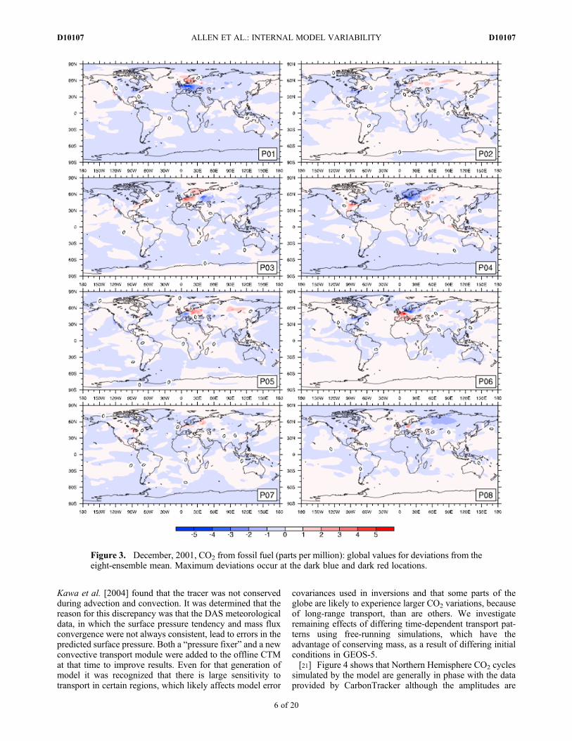
concentrations in eight simulations by the same model differby a factor of 3. Figures 2 and 3 depict global values for thedeviations from the ensemble mean CO2 from fossil fuel inparts-per-million for the first month of the simulation (Jan-uary, 2000), and for the last month (December 2001),respectively. A quantitative description of the percentdeviations (shown as fractional amounts) can be found inTable 1. The largest maximum deviation from the mean forJanuary, 2000 (+21%) occurs in simulation P04 in the regionof Germany/Poland, and the smallest (7%) in P06—a dis-crepancy of a factor of 3. In December 2001, the maximumdeviation (+22.5%) occurs at the same location in simulationP06, in which the region showed a negative deviation inJanuary 2000. The smallest maximum deviation for thismonth (7%) is also approximately 1/3 of the largest. Meandeviation from the mean for all simulations, while low(0.005% to 0.26%), and somewhat variable (least andgreatest differ by two orders of magnitude in January 2000and one order of magnitude in December 2001), neverthe-less persists from the first month of the run until the last.[17] In their CO2 observational network Tans et al. [1989]

discovered that regionally significant CO2 sources and sinksare needed to maintain small but persistent spatial gradients,


3 of 20

given that atmospheric circulation and mixing are constantlyworking to homogenize the atmosphere; and that whilemeasurement sites closer to source regions are needed tobetter determine the effect of sources on the global carbonbudget, such measurements do introduce a bias effect. Forexample, if transport is less vigorous during the seasonwhen a surface region is a source rather than when it is asink, a positive net annual concentration anomaly will result.Nevertheless, it is important to include measurements inregions of sources and sinks, as they will become helpful for

monitoring CO2 emissions more so than the measurementsin more stable regions which give information primarilyabout trends of the background state. These measurementswill need to be accounted for in innovative ways, however,in order to increase both observational and model accuracy.[18] Internal model variability of transport can also affect

the flow of air masses differently in regions of sources andsinks to atmospheric CO2. Even with specified emissionsand uptake, there are some regions in which atmosphericCO2 distribution is strongly affected by transport patterns.

Figure 1. January 2000 lowest atmospheric layer concentrations of CO2 from fossil fuel in parts per mil-lion for the eight model simulations. Spatial differences in concentration represent differences in the result-ing average January values due to the diverse initial meteorological conditions among the simulations.


4 of 20

3.2. CO2 Cycle Phasing and Amplitude

[19] The uptake and release of atmospheric CO2 withvarious surface carbon reservoirs imparts a strong signal onobserved atmospheric CO2 concentrations on time scalesranging from days to years [Erickson et al., 1996]. It isknown that the overall seasonal cycle of all sources andsinks is dominated by variation in atmosphere-terrestrial

biosphere CO2 exchange [Heimann and Keeling, 1986;Erickson et al., 1996], but ongoing studies evidence thecontinually emerging fingerprint of fossil fuel emissions aswell on both global and regional cycles [Keeling et al., 1989;Gurney et al., 2005; Erickson et al., 2008].[20] In a CO2 transport simulation using GEOS-4 and the

NASA finite volume data assimilation system (FVDAS)fields to drive an offline chemical transport model (CTM),

Figure 2. January, 2000, CO2 from fossil fuel (parts per million): global values for deviations from theeight-ensemble mean. Maximum deviations occur at the dark blue (up to �5 ppm) and dark red (up to+5 ppm) locations.


5 of 20

Kawa et al. [2004] found that the tracer was not conservedduring advection and convection. It was determined that thereason for this discrepancy was that the DAS meteorologicaldata, in which the surface pressure tendency and mass fluxconvergence were not always consistent, lead to errors in thepredicted surface pressure. Both a “pressure fixer” and a newconvective transport module were added to the offline CTMat that time to improve results. Even for that generation ofmodel it was recognized that there is large sensitivity totransport in certain regions, which likely affects model error

covariances used in inversions and that some parts of theglobe are likely to experience larger CO2 variations, becauseof long-range transport, than are others. We investigateremaining effects of differing time-dependent transport pat-terns using free-running simulations, which have theadvantage of conserving mass, as a result of differing initialconditions in GEOS-5.[21] Figure 4 shows that Northern Hemisphere CO2 cycles

simulated by the model are generally in phase with the dataprovided by CarbonTracker although the amplitudes are

Figure 3. December, 2001, CO2 from fossil fuel (parts per million): global values for deviations from theeight-ensemble mean. Maximum deviations occur at the dark blue and dark red locations.


6 of 20

underestimated by the model at both Romania and Kazakhstan,and the June 2000 minimum for the CarbonTracker datain Romania leads the simulations by one month. Modelamplitudes at Park Falls, Wisconsin overestimate the Car-bonTracker data especially during the latter half of 2000and at the July–August minimum in 2001. At Mauna Loa,the models show slightly larger amplitudes but very similarphasing for 2000, and very near matches for amplitude andphase in 2001. These similarities among model runs andobservations suggest that both physical parameterizationsand CO2 flux sources are administered reasonably for theNorthern Hemisphere and that the differing initial conditionsin meteorology in the eight ensemble runs have little effecton the realization of the CO2 cycle at these latitudes.[22] Results for the Southern Hemisphere in Figure 5

show marked differences in both amplitude and phasingamong the models and with regard to the observational dataset. In fact, the number of months difference in phase formodels compared to observations differs according to lati-tude—the farther north in the southern hemisphere, the far-ther out of phase. For example, at Easter Island (coordinates:27.15S, 109.45W), the simulations lead the observations byfour months; at Cape Grim, Tasmania (40.68S, 143.68E), bythree months; at Maquarie Island (54.48S, 158.97E), by onemonth; and at the South Pole by less than a month.[23] To better understand the cause of the widely differing

model simulations for Cape Grim, the FFT procedure per-formed on the total CO2 cycle for all of the locations in thestudy was employed for each component of the total CO2

concentration at Cape Grim and compared to the Carbon-Tracker data for the region. Figure 6 shows that biomassburning has little effect on the cycle, that the ocean cycleleads the observations by three months (as found by Kawaet al. [2004]), and that both the terrestrial biosphere (CASA)and the fossil fuel cycles are affected quite differently by thepropagation of the differing initial meteorological conditionsapplied to each model ensemble member. It should be noted,however, that local discrepancies in the CASA data itselfmay contribute to the differences seen among the simulationsfor this component—a point demonstrated by Masarieet al. [2011] when bias was introduced into Park Falls,Wisconsin data input into a CO2 flux simulation.[24] The fossil fuel component of the CO2 cycle here is the

only component that is more or less in phase with theobservations (especially for ensemble members P01 andP02, identical for this component and represented by the red

curve), which is consistent with Kawa et al. [2004]. Theamplitude of this signal is approximately 30% of the totalCO2 signal in the observations, consistent with Ericksonet al. [2008] in which the National Center for AtmosphericResearch (NCAR) Community Atmosphere Model, Version4.0, was run with a monthly fossil fuel flux data set fromAndres et al. [1996]. These findings suggest that althoughinterhemispheric transport of CO2 from fossil fuel from theNorthern Hemisphere to the Southern Hemisphere mayaffect the phase of the CO2 cycle in the Southern Hemi-sphere; internal model variability still obstructs the truefossil fuel CO2 signal at specific sites in the SouthernHemisphere.

3.3. Interhemispheric Exchange Time

[25] Observations of long-lived tracers indicate that the timerequired for mixing tropospheric air between the Northernand Southern Hemisphere extratropics is on the order of0.61–1.4 year [Kawa et al., 2004; Denning et al., 1999;Bowman and Cohen, 1997; Heimann and Keeling, 1986].Using the adapted Bowman and Cohen equations (1) and (2)above, we obtain the values shown in Table 2 for the lowestatmospheric layer concentrations of CO2 for each of the eightsimulations from 2000 to 2001 and for each of the four dif-ferent sources of CO2. Remaining mindful that this boxmodel calculation accounts only for Northern Hemispheresources, we note the following interhemispheric transportvalues obtained. For Total CO2 (CO2TOT), transport timeranges from 0.93 yr. to 1.06 yr, a value slightly less than thatof Heimann and Keeling [1986], but in keeping withDenning et al. [1999]. The CO2 from fossil fuel burning(CO2FF) transport time range is 0.442 yr. to 0.456 yr.—significantly less than values seen for total CO2 in this or inany other model. Terrestrial Biosphere CO2 (CASA) trans-port time shows the widest range from �9.26 yr. to 1.43 yrs.(The two negative source values here are due to the fact thatCASA is artificially balanced annually to be close to zero,and thus gives source values slightly above or slightly belowzero). Four of the terrestrial biosphere simulations (P03,P04, P05, and P07), however, show transport time between0.01 yr. and 0.1 yr. (approximately 3–37 days). Ocean CO2

(CO2OCN) values represent Northern Hemisphere sinks andresulting removal of CO2 from the Southern Hemispherewith “transport” time of 1.5 yr. Differences in transporttimes among the various constituent source/sinks of total

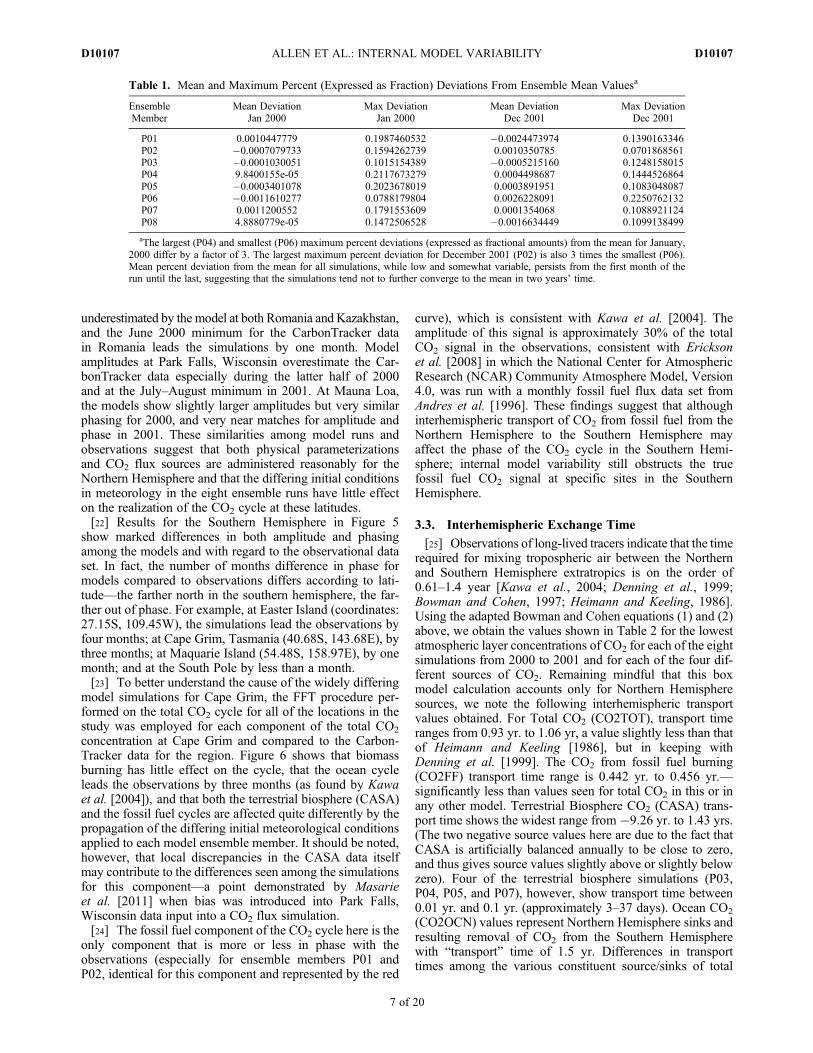
Table 1. Mean and Maximum Percent (Expressed as Fraction) Deviations From Ensemble Mean Valuesa

EnsembleMember

Mean DeviationJan 2000

Max DeviationJan 2000

Mean DeviationDec 2001

Max DeviationDec 2001

P01 0.0010447779 0.1987460532 �0.0024473974 0.1390163346P02 �0.0007079733 0.1594262739 0.0010350785 0.0701868561P03 �0.0001030051 0.1015154389 �0.0005215160 0.1248158015P04 9.8400155e-05 0.2117673279 0.0004498687 0.1444526864P05 �0.0003401078 0.2023678019 0.0003891951 0.1083048087P06 �0.0011610277 0.0788179804 0.0026228091 0.2250762132P07 0.0011200552 0.1791553609 0.0001354068 0.1088921124P08 4.8880779e-05 0.1472506528 �0.0016634449 0.1099138499

aThe largest (P04) and smallest (P06) maximum percent deviations (expressed as fractional amounts) from the mean for January,2000 differ by a factor of 3. The largest maximum percent deviation for December 2001 (P02) is also 3 times the smallest (P06).Mean percent deviation from the mean for all simulations, while low and somewhat variable, persists from the first month of therun until the last, suggesting that the simulations tend not to further converge to the mean in two years’ time.


7 of 20

CO2 may be due to their proximal distribution about theequator.3.3.1. Vertical Transport[26] Denning et al. [1998], found that differences in ver-

tical structure among general circulation models dominatethe differences in true interhemispheric exchange. Toinvestigate differences in vertical structures developed frominitial conditions that may be responsible for similar trans-port discrepancies within the GEOS-5 model, we examinetransport time at the 500 mb level. Table 3 shows the out-come of these calculations. The results show a wider rangeof values at this level than at the surface level, suggesting

large discrepancies in the vertical mixing in each of thesimulations. In this case, Total CO2 (500TOT), transporttime ranges from 0.83 yr. to 0.95 yr. For CO2 from fossilfuel burning (500FF), the transport time range is about twiceas long at the 500 mb level than it is at the surface: 0.83 yr to1.09 yr and represents a 31% increase from the smallest tothe largest value as compared to only a 3% increase fromsmallest to largest surface values. Terrestrial Biosphere CO2

(CASA) transport time again shows the widest range at thislevel from 0.167 yr to 1.58 yr (rejecting the 11 yr. outlier).The range of ocean CO2 (CO2OCN) values range from0.446 yrs to 1.03 yrs.

Figure 4. Northern Hemisphere total CO2 (composite of sources from ocean, terrestrial biosphere, fossilfuel emissions and biomass burning) seasonal amplitude 2000–2001, CarbonTracker versus GEOS-5ensemble (note different ranges for different y-axes). Northern Hemisphere CO2 cycles simulated by themodel are generally in phase with the CarbonTracker data although the amplitudes are underestimatedby the model at both Romania (44.17�N, 26.68�E) and Kazakhstan (44.45�N, 75.57�E), and the June2000 minimum for observations in Romania leads the model simulations by one month. Model amplitudesat Park Falls, Wisconsin (45.95�N, 90.27�W) overestimate observations especially during the latter half of2000 and at the July–August minimum in 2001. At Mauna Loa (19.53�N, 155.58�W), the model simula-tions show slightly larger amplitudes but very similar phasing for 2000, and very near matches for ampli-tude and phase in 2001.


8 of 20

[27] In the TRANSCOM studies conducted by Law et al.[1996], results from twelve atmospheric transport modelswere collected and analyzed for differences in representationof CO2 transport. Within this study, an assessment of thelarge discrepancy in interhemispheric concentration differ-ences between the model that produced the largest differenceand the one that produced the smallest revealed that therewere differences in the models’ subgrid scale vertical trans-port mechanisms, and were the result of the different para-meterizations used and the different numerical diffusionproperties of the advection schemes in the two models. Inthe study it was noted that one of the models investigatedappeared to have weak vertical mixing throughout the tro-posphere while another had weak mixing out of its surfacelayer. In both models, this resulted in higher surface con-centrations. While the range of transport times found in the

different simulations of the single GEOS-5 model is notquite as large a range as that of the Law et al. [1996] multiplemodel comparison, it suggests that surface mixing strengthover the time span of a model run may vary for sensitiveregions in the model. Additionally, the observation that thetransport times for each component of the CO2 signal rangefrom 0.01 yr to 1.58 yr indicates that while the variouscomponents undergo essentially the same mixing processes,there are differences in the resulting spatial structure of theCO2 tracer that are being driven by mixing processes (i.e.,timing and strengths of fronts and planetary waves). To gaininsight into the effect of transport processes on atmosphericflow from the Northern Hemisphere to the Southern Hemi-sphere, a 3D time-varying flow analysis was performedusing a method of integration-based flow analysis.

Figure 5. Southern Hemisphere total CO2 seasonal amplitude 2000–2001 Observations versus GEOS-5ensemble. CO2 cycle results for the Southern Hemisphere show marked differences in both amplitude andphasing among the models and with regard to the CarbonTracker data sets. At Easter Island (27.15�S,109.45�W) the simulations lead the observations by four months; at Cape Grim, Tasmania (40.68�S,143.68�E), by three months; at Maquarie Island (54.48�S, 158.97�E), by one month; and at the South Pole(89.98�S, 24.8�W) by less than a month.


9 of 20

3.4. Flow Into Mauna Loa

[28] In their twelve-model inter-comparison project, Lawet al. [1996] determined that large-scale winds account for

about half the difference between model results, and thatadditional attribution must lay in differences in the subgridscale vertical transport parameterization and diffusion

Table 2. Northern Source (SN in mol/mol) and Interhemispheric Transport Time (yrs), Surfacea

SN CO2TOT Tau CO2TOT SN CO2FF Tau CO2FF SN CO2CASA Tau CO2CASA SN CO2OCN Tau CO2OCNEnsembleMember

4.86E-06 0.951 8.76E-06 0.445 1.12E-07 1.43 �1.26E-06 1.32 P014.61E-06 1.06 8.58E-06 0.456 �7.00E-09 �9.26 �1.21E-06 1.39 P024.95E-06 0.939 8.80E-06 0.444 3.26E-07 0.0601 �1.24E-06 1.32 P034.89E-06 0.965 8.74E-06 0.449 1.71E-07 0.105 �1.02E-06 1.58 P045.10E-06 0.926 8.89E-06 0.441 2.69E-07 0.0156 �1.22E-06 1.38 P054.75E-06 1.01 8.81E-06 0.444 �9.40E-09 �2.77 �1.16E-06 1.43 P064.78E-06 0.970 8.83E-06 0.437 1.47E-07 0.0545 �1.20E-06 1.26 P074.95E-06 0.952 8.83E-06 0.442 1.06E-07 0.313 �1.11E-06 1.54 P08

aTotal CO2, CO2 from fossil fuel, terrestrial biosphere CO2, and ocean CO2 for all eight simulations are shown for the lowest atmospheric layer in themodel. Northern Hemisphere source CO2 (SN) is given in mol/mol values. Interhemispheric transport time Tau is given in year fraction.

Figure 6. Cape Grim (40.68�S, 143.68�E) components of the CO2 cycle. Biomass burning has littleeffect on the cycle, the ocean leads the observations by three months (as in Kawa et al. [2004]), and boththe terrestrial biosphere (CASA) and the fossil fuel cycles are affected quite differently by the internalmodel variability with regard to the development of the differing initial meteorological conditions appliedto each ensemble member.


10 of 20

properties of their advection schemes. Since the Mauna Loaobservatory, at its remote location, has traditionally provideda reliable account of the background state of atmosphericCO2, we begin by examining large-scale wind flow pathshere using an integration-based flow analysis.[29] To determine the historical path of a given particle

arriving at Mauna Loa, equation (3) in section 2.3 is solvedusing a negative time step (=14,400 s, i.e., 4 hours), and theintegration progresses backward through space and time. Inthese analyses the lower 13 pressure layers (approximately1013 hPa to 820 hPa if the lowest layer is at sea level) werequeried for, and particle tracers initialized from each of thosequeried points. This vertical limit was selected such thatsome vertical transport is shown along with the horizontal,but not so much as to make the plot so dense as to beincomprehensible. The destination location was set to thelower 13 pressure layers of Mauna Loa.[30] Observations from CarbonTracker (Figure 4) showed

that maximum CO2 mixing ratios occur in May of 2000 andMay of 2001 and that minimum values occur in September2000 and 2001. Aside from an increase in the amplitude ofCO2 at Mauna Loa from 2000 to 2001, no remarkable dif-ferences in transport are seen from one year to the next atthis location. We present examples of particle flow withthree-month lead time into Mauna Loa for the year 2001 forthese months. All simulations at this location estimate wellboth amplitude and phasing of the CO2 cycle for the period.For the remainder of the figures in this paper, each colorrepresents the trajectory computed by each model simula-tion. Opacity corresponds to time elapsed—the more trans-parent, the longer temporal displacement.[31] As can be seen in Figures 7 and 8 (May and Sep-

tember, 2001 particle flow with three-months’ lead time intoMauna Loa, respectively), the Hadley circulation contributesto the interhemispheric transport through its seasonal oscil-lation [Bowman and Cohen, 1997]. In response to seasonalsolar heating, the Intertropical Convergence Zone (ITCZ)moves northward and southward (toward the warmer hemi-sphere), allowing air that was previously in one Hadley cellto be carried upward and poleward in the other Hadley cell.Additionally, transport within convective cells (such as thosecharacteristic of tropical cyclones) increases the rate atwhich tracers are transported between adjacent convectiverolls [Young et al., 1989]. Therefore, it might be assumedthat the CO2 cycle at locations receiving Hadley cell airshould be affected by surface sources in the other hemi-sphere. Mauna Loa is one such location.

[32] At three months in advance of May 2001 arrival,Figure 7 shows that sources of air entering Mauna Loainclude air from vortices located at 30�S. These sources areswept into the equatorial current and then drawn into thePacific vortex before entering Mauna Loa. Air particles thatbegin in the Southern Hemisphere follow a vertical pathwayinto the Northern Hemisphere. At one month lead time,particles are generally near the northeastern U.S. coastline.From there, they either follow the jet stream to the Atlanticand over Eurasia, to enter from the Pacific, or they travelsouthward over the Atlantic, as in P03-P08, to be drawn intoMauna Loa across North America.[33] In Figure 8, arrival at Mauna Loa in September, 2001

with three month lead time is shown. As the ITCZ and the jetstream move south, the jet stream plays less a role in anairstream’s travel into Mauna Loa than it does in May. Atthree months in advance of arrival, southern sources of airalso undergo less activity in September than they do in May.Interhemispheric exchange occurs mainly in the regionbetween eastern Africa and Indonesia. Northern paths orig-inate in North America and the Atlantic Ocean. No SouthernHemisphere sources appear in P07. Few are included in P01.Again, the interhemispheric transport is seen to be accom-plished mainly by travel in the upper atmospheric layers.[34] In the case of the CO2 cycle at Mauna Loa, all eight

simulations are in phase with observations and within a fewppm of the amplitude. In both May and September, allsimulations follow similar one-month lead time paths toMauna Loa. Northern Hemisphere sources (eastern Canadaand the Atlantic Ocean) three months before arrival aresimilar for all models while Southern Hemisphere sourceseither vary or are not present. This suggests that NorthernHemisphere sources of air (and consequently, CO2) have alarger effect on the amplitude and the phasing of the carboncycle at Mauna Loa than Southern Hemisphere sources do.Thus, varying initial meteorological conditions in GEOS-5does not produce a large effect on CO2 concentrations atMauna Loa. Northern Hemisphere sources, which are fardistant from Mauna Loa, are well-mixed by the time theyreach Mauna Loa, so they affect concentration there simi-larly in all simulations. Southern Hemisphere sources arefew, so variations in transport times for particles from theselocations have little effect on CO2 concentrations at MaunaLoa.

3.5. Flow Into Cape Grim

[35] At Cape Grim, Tasmania, observations showed thatminimum CO2 mixing ratios occur in April of 2000 and May

Table 3. Northern Source (SN in mol/mol) and Interhemispheric Transport Time (yrs), 500 mba

Sn 500TOT Tau 500TOT Sn 500FF Tau 500FF Sn 500CASA Tau 500CASA Sn 500OCN Tau 500OCNEnsembleMember

3.90E-06 0.894 8.43E-06 0.831 �2.66E-08 0.519 �2.18E-06 0.482 P013.79E-06 0.952 7.40E-06 0.887 �1.28E-08 �0.188 �2.10E-06 0.446 P024.08E-06 0.902 8.51E-06 0.821 �3.72E-08 0.167 �2.32E-06 0.469 P033.75E-06 0.954 6.50E-06 1.07 �6.20E-09 �0.581 �1.05E-06 1.03 P043.77E-06 0.946 6.39E-06 1.09 �4.60E-09 �2.30E-14 �1.11E-06 0.995 P053.65E-06 0.929 6.44E-06 1.06 2.00E-10 11.0 �1.03E-06 1.02 P064.08E-06 0.833 7.30E-06 0.936 �5.08E-08 0.402 6.98E-01 �1.47E-06 P073.91E-06 0.881 6.76E-06 1.02 �5.60E-09 �0.0714 �1.62E-06 0.691 P08

aTotal CO2, CO2 from fossil fuel, terrestrial biosphere CO2 and ocean CO2 for all eight simulations are shown for the 500 mb atmospheric layer in themodel. Units are as in Table 2.


11 of 20

Figure 7. May 2001 arrivals into Mauna Loa (19.53�N, 155.58�W) with three month lead times. Opacitycorresponds to time elapsed—the more transparent, the longer temporal displacement. At three monthsbefore arrival, sources of air entering Mauna Loa include air from vortices located at 30�S. These sourcesare swept into the equatorial current and then drawn into the Pacific vortex before entering Mauna Loa.Air particles that begin in the Southern Hemisphere follow a vertical pathway into the NorthernHemisphere.


12 of 20

Figure 8. September 2001 arrivals into Mauna Loa (19.53�N, 155.58�W) with three month lead times.As the ITCZ and the jet stream move south, the jet stream plays less a role in an airstream’s travel intoMauna Loa than it does in May. Interhemispheric exchange occurs mainly in the region between easternAfrica and Indonesia. Northern paths originate in North America and the Atlantic Ocean. No SouthernHemisphere sources appear in P07. Few are included in P01.


13 of 20

of 2001 and that maximum values occur in September 2000and 2001. This cycle is the reverse of that of Mauna Loa.[36] Since this is where the largest discrepancies in the

CO2 cycle were found among the GEOS-5 simulations, weinvestigate the large-scale processes in this region in com-parison with those at the more stable Mauna Loa site usingflow analysis into this region in May and September. Itshould be noted that our results are not the first to showprominent differences between observations and modeloutput for tracer concentrations in the Australian region.Several studies have shown southern midlatitude tracerconcentration aberrations in their findings. A few aredescribed in the following section.

3.6. Known Australian Regional Aberrations

[37] The Conway et al. [1994] study evaluating CO2 flaskdata noted that in the Southern Hemisphere, Cape Grim,Tasmania concentrations of CO2 always fell below thatwhich was calculated using the cubic polynomial fit curvewhich approximated well the northern to southern hemi-sphere CO2 gradient. This location consistently showed thelowest annual mean in the observational network with valuesslightly lower even than those at the South Pole.[38] In the Law et al. [2003] TRANSCOM 3 CO2 inver-

sion comparison, data network tests performed showed thatonly the Australian region source estimates varied over amuch larger range than that given by the established controlcase uncertainty estimate. By their estimation, the data sug-gested that the assumed spatial pattern of sources in Aus-tralia in the 16 models compared was incorrect—that largersources were required in the northern part of the continentrelative to the south. An alternative explanation, that therecould be an error in transport, was deemed less likely sinceall transport models behaved in the same way. We proposethat this region may indeed pose a transport challenge formany models based on internal model variability.[39] A look at the flow patterns of individual ensemble

member simulations for May and September, 2001, at threemonth lead time reveals significant differences in particlepathways into Cape Grim. In Figure 9, May 2001 arrivalsinto Cape Grim with three month lead time, simulationsshow streamlines coming primarily from the Atlantic, Africaand southern Asia. P01, P02, P04 and P07 include pathstaken through North America. Simulations P05-P08 includean Atlantic vortex into which Northern Hemisphere air isdrawn to be delivered to the Southern Hemisphere. Long-range particles are carried primarily in the uppermost verticallayer (�820 hPa). Figure 10 shows September 2001 arrivalsinto Cape Grim with three month lead time. Peak CO2

values for the observation data occur during this month,while all of the GEOS-5 model simulations are in the middleof CO2 decline here. Lowest CO2 fossil fuel values occur inSeptember 2001 for P08. This is also the only simulation forwhich the Southern Ocean air current is the only source ofairstreams. Highest GEOS-5 model values during this monthobtain for P01, P04, P05. The most varied paths to CapeGrim are taken by simulations P02, P03, P06 and P07.Interhemispheric transport paths are seen mainly in the upperatmospheric layers. We recall that the model simulationswhose fossil fuel emission component most closely matchedthe phasing of the Cape Grim CO2 cycle were P01 and P02

and that these were the only two to show residence insoutheast Asia, a known major emitter of fossil fuel CO2.

3.7. Interannual Variability

[40] In addition to the variability among the GEOS-5model simulations for Cape Grim for each of the two yearssimulated, a notable amount of interannual variability waspresent. This result is consistent with the findings of Conwayet al. [1994] who report significant interannual variations inthe interhemispheric gradient of atmospheric CO2 in theobservation network. Figure 11 depicts May 2000 (top) and2001 (bottom) arrivals into Cape Grim with one month leadtime. Streams from blue (P03), purple (P02), red (P01) andcyan (P04) arrive latest, since these come from the largestdistances away. In the 2000 simulation, black (P08) is in theAfrican cape one month before arrival, it then travels arounda South Pacific vortex before entering Cape Grim. In the2001 simulation, black (P08) spins in a tight vortex aroundTasmania while the other simulations rotate nearer thesouthern Australian coast. These interannual variations maybe due to seasonal cyclonic activity in the Indian Ocean[Bowman and Cohen, 1997] or to climatic oscillations suchas the El Niño/La Niña cycle. In either case, this variabilityis seen in only some of the simulations suggesting thatmeteorological differences from year to year represent onlypart of the variability in the simulations.[41] September 2000, 2001 arrivals into Cape Grim with

one month lead time are shown in Figure 12. Here we seemore interannual variability in more of the simulations. In2000, black (P08) and yellow (P06) curl around the Africancape one month before arrival, while in 2001, red (P01) andblue (P03) show this pattern. Blue (P03), cyan (P04) andgreen (P05) spin near the southern Australian coast in 2000,but only green (P05) does this in 2001.

3.8. El Niño/La Niña

[42] Much interannual variability is related to natural cli-mate fluctuations. For instance, the effect of El Niño/LaNiña, can be large compared to the effect of changes inannual fossil fuel emissions [Conway et al., 1994]. In fact,the terrestrial biosphere releases more CO2 to the atmo-sphere during El Niño events, which results in increasedCO2 growth rates during these events [Keeling et al., 1989]and La Niña events can have a slightly less and oppositeeffect. Results from Heimann and Reichstein [2008] showthat the El Niño Southern Oscillation (ENSO) is in a nega-tive phase (La Niña) in the years 2000–2001 and that duringthis time, the phase is becoming slightly less negative.Global background atmospheric CO2 concentration risesonly slightly (approximately 0.05 ppm) over this period.

4. Conclusions

[43] In regions of high CO2 emissions due to fossil fuelburning, large differences among the simulations appear forboth the first month and the last month of the ensemblesimulation. Thus, individual simulations of an eight-memberensemble do not stabilize within a period of two years.[44] The phasing of the CO2 cycle at Northern Hemi-

sphere locations in all of the ensemble members is similar tothat of the CarbonTracker collection of observations, but inthe southern hemisphere, GEOS-5 model cycles are out of


14 of 20

phase by as much as four months, and large variations occurbetween the ensemble members. The most extreme differ-ences occur among the ensemble and observational data inthe Cape Grim region with regard to CO2 uptake and respi-ration of the terrestrial biosphere and CO2 emissions due to

fossil fuel burning. While the amplitude of the cycle of theocean and the terrestrial biosphere represent the largest per-centages of the total CO2 cycle at Cape Grim, the phasing offossil fuel CO2 at 30–40% of the amplitude most closelyfollows the phase of the CO2 total at this location.

Figure 9. May 2001 arrivals into Cape Grim (40.68�S, 143.68�E) with three month lead time. Simula-tions show streamlines coming primarily from the Atlantic, Africa and southern Asia. P01, P02, P04and P07 include paths taken through North America. Simulations P05-P08 include an Atlantic vortex intowhich Northern Hemisphere air is drawn to be delivered to the Southern Hemisphere. Long-range particlesare carried primarily in the uppermost vertical layer.


15 of 20

[45] These findings suggest that although interhemispherictransport of CO2 from fossil fuel produced in the NorthernHemisphere to the Southern Hemisphere may affect thephase of the CO2 cycle in the Southern Hemisphere, internalmodel variability still obstructs the true CO2 signal at

specific sites in the Southern Hemisphere. Potential expla-nations for these discrepancies may lie in the robustness ofthe terrestrial biosphere or ocean flux data, model tuning orparameterization for the Southern Hemisphere; or in thathigher concentrations of CO2 in the Northern Hemisphere

Figure 10. September 2001 arrivals into Cape Grim (40.68�S, 143.68�E) with three month lead time.Peak CO2 values for the CarbonTracker data occur during this month, while all of the GEOS-5 modelsimulations are in the middle of CO2 decline here. Lowest CO2 fossil fuel values occur in September2001 for P08. This is also the only model for which the Southern Ocean air current is the only sourceof airstreams. Highest GEOS-5 model values during this month obtain for P01, P04, P05. The most variedpaths to Cape Grim are taken by simulations P02, P03, P06 and P07.


16 of 20

Figure 11. May (top) 2000 and (bottom) 2001 arrivals into Cape Grim (40.68�S, 143.68�E) with onemonth lead time. Streams from blue (P03), purple (P02), red (P01) and cyan (P04) arrive latest, since thesecome from the largest distances away. In the 2000 simulation, black (P08) is in the African cape onemonth before arrival, then travels around a South Pacific vortex before entering Cape Grim. In the 2001simulation, black (P08) spins in a tight vortex around Tasmania while the other simulations rotate nearerthe southern Australian coast. (Additional simulations: P05, green; P06, yellow; and P07, ochre).


17 of 20

Figure 12. September (top) 2000 and (bottom) 2001 arrivals into Cape Grim (40.68�S, 143.68�E) withone month lead time. Here we see more interannual variability in more of the simulations. In 2000, black(P08) and yellow (P06) curl around the African cape one month before arrival, while in 2001, red (P01)and blue (P03) show this pattern. Blue (P03), cyan (P04) and green (P05) spin near the southern Australiancoast in 2000, but only green (P05) does this in 2001. (Additional simulations: P02, purple; P07, ochre).


18 of 20

affect amplitude and phasing in the Southern Hemispheremore than circulation affects it in any location.[46] It is clear that some parts of the globe experience

larger CO2 variations, due to long-range transport, than doothers. Measurements in those regions might be moreappropriate for monitoring CO2 emissions than the mea-surements in the more stable regions, which are most effi-cient at monitoring the background state or trend.Furthermore, surface mixing strength over the time span of amodel run may vary for sensitive regions in the model, andthe large differences in the transport times for each compo-nent of the CO2 may indicate that there are structural differ-ences in the mixing processes of the various simulations. Weconclude that time-dependent transport patterns, especiallybetween the Northern and the Southern Hemispheres, affectinternal model variability significantly.

[47] Acknowledgments. We acknowledge support from the NASACarbon Cycle Science and the NASA High-End Computing Program. Thisresearch used resources of the National Center for Computational Sciencesat Oak Ridge National Laboratory (ORNL).

ReferencesAndres, R. J., G. Marland, I. Fung, and E. Matthews (1996), A 1� � 1� dis-tribution of carbon dioxide emissions from fossil fuel consumptionand cement manufacture, 1950–1990, Global Biogeochem. Cycles, 10,419–429, doi:10.1029/96GB01523.

Baker, D. F., et al. (2006), TransCom 3 inversion intercomparison:Impact of transport model errors on the interannual variability of regionalCO2 fluxes, 1988–2003, Global Biogeochem. Cycles, 20, GB1002,doi:10.1029/2004GB002439.

Bowman, K. P., and P. J. Cohen (1997), Interhemispheric exchange byseasonal modulation of the Hadley Circulation, J. Atmos. Sci., 54,2045–2059, doi:10.1175/1520-0469(1997)054<2045:IEBSMO>2.0.CO;2.

Chou, M.-D., and M. J. Suarez (1999), A solar radiation parameterizationfor atmospheric studies, NASA Tech. Rep., 104606, vol. 15, 40 pp.

Chou, M.-D., M. J. Suarez, X. Z. Liang, and M. M.-H. Yan (2001), A ther-mal infrared radiation parameterization for atmospheric studies, NASATech. Rep., 104606, vol. 19, 56 pp.

Conway, T. J., P. P. Tans, L. S. Waterman, K. W. Thoning, D. R. Kitzis,K. A. Masarie, and N. Zhang (1994), Evidence for interannual variabil-ity of the carbon cycle from the National Oceanic and AtmosphericAdministration/Climate Monitoring and Diagnostics Laboratory GlobalAir Sampling Network, J. Geophys. Res., 99(D11), 22,831–22,855,doi:10.1029/94JD01951.

Denning, A. S., P. J. Rayner, R. M. Law, and K. R. Gurney (1998), Atmo-spheric Tracer Transport Model Intercomparison Project (TransCom),IGBP/GAIM Rep. 4, NCAR, Boulder, Colo.

Denning, A. S., et al. (1999), Three-dimensional transport and concentra-tion of SF6—A model intercomparison study (TransCom 2), Tellus,Ser. B, 51, 266–297, doi:10.1034/j.1600-0889.1999.00012.x.

Erickson, D. J., III, P. J. Rasch, P. P. Tans, P. Friedlingstein, P. Ciais,E. Maier-Reimer, K. Kurz, C. A. Fischer, and S. Walters (1996), The sea-sonal cycle of atmospheric CO2: A study based on the NCAR Commu-nity Climate Model (CCM2), J. Geophys. Res., 101, 15,079–15,097.

Erickson, D. J., III, R. T. Mills, J. Gregg, T. J. Blasing, F. M. Hoffman,R. J. Andres, M. Devries, Z. Zhu, and S. R. Kawa (2008), An estimate ofmonthly global emissions of anthropogenic CO2: Impact on the seasonalcycle of atmospheric CO2, J. Geophys. Res., 113, G01023, doi:10.1029/2007JG000435.

Gurney, K. R., et al. (2002), Towards robust regional estimates of CO2sources and sinks using atmospheric transport models, Nature, 415,626–630, doi:10.1038/415626a.

Gurney, K. R., Y.-H. Chen, T. Maki, S. R. Kawa, A. Andrews, and Z. Zhu(2005), Sensitivity of atmospheric CO2 inversions to seasonal and inter-annual variations in fossil fuel emissions, J. Geophys. Res., 110,D10308, doi:10.1029/2004JD005373.

Heimann, M., and C. D. Keeling (1986), Meridional eddy diffusion modelof the transport of atmospheric carbon dioxide: 1. Seasonal carbon cycleover the tropical Pacific Ocean, J. Geophys. Res., 91, 7765–7781,doi:10.1029/JD091iD07p07765.

Heimann, M., and M. Reichstein (2008), Terrestrial ecosystem carbondynamics and climate feedbacks, Nature, 451, 289–292, doi:10.1038/nature06591.

Kawa, S. R., D. J. Erickson III, S. Pawson, and Z. Zhu (2004), Global CO2transport simulations using meteorological data from the NASA dataassimilation system, J. Geophys. Res., 109, D18312, doi:10.1029/2004JD004554.

Keeling, C. D., R. B. Bacastow, A. E. Bainbridge, C. A. Ekdahl, P. R.Guenther, and L. S. Waterman (1976), Atmospheric carbon dioxide var-iations at Mauna Loa Observatory, Hawaii, Tellus, 28, 538–551,doi:10.1111/j.2153-3490.1976.tb00701.x.

Keeling, C. D., S. C. Piper, and M. Heimann (1989), A three-dimensionalmodel of atmospheric CO2 transport based on observed winds: 4. Meanannual gradients and interannual variations, in Aspects of Climate Vari-ability in the Pacific and the Western Americas, Geophys. Monogr.Ser., vol. 55, edited by D. H. Peterson, pp. 305–363, AGU, Washington,D. C., doi:10.1029/GM055p0305.

Kendall, W., J. Wang, M. Allen, T. Peterka, J. Huang, and D. Erickson(2011), Simplified parallel domain traversal, paper presented at SC ’11:International Conference for High Performance Computing, Networking,Storage and Analysis, ACM, New York.

Law, R. M., et al. (1996), Variations in modeled atmospheric transport ofcarbon dioxide and the consequences for CO2 inversions, Global Biogeo-chem. Cycles, 10, 783–796, doi:10.1029/96GB01892.

Law, R. M., et al. (2003), TransCom 3 CO2 inversion intercomparison: 2.Sensitivity of annual mean results to data choices, Tellus. Ser. B, 55,580–595.

Law, R. M., et al. (2008), TransCom model simulations of hourly atmo-spheric CO2: Experimental overview and diurnal cycle results for 2002,Global Biogeochem. Cycles, 22, GB3009, doi:10.1029/2007GB003050.

Lin, S.-J. (2004), A “vertically Lagrangian” finite-volume dynamical corefor global models, Mon. Weather Rev., 132, 2293–2307, doi:10.1175/1520-0493(2004)132<2293:AVLFDC>2.0.CO;2.

Lock, A. P., A. R. Brown, M. R. Bush, G. M. Martin, and R. N. B. Smith(2000), A new boundary layer mixing scheme. Part I: Scheme descriptionand single-column model tests, Mon. Weather Rev., 128, 3187–3199,doi:10.1175/1520-0493(2000)128<3187:ANBLMS>2.0.CO;2.

Louis, J., M. Tiedtke, and J. Geleyn (1982), A short history of the PBLparameterization at ECMWF, paper presented at Workshop on PlanetaryBoundary Layer Parameterization, ECMWF, Reading, U. K.

Masarie, K. A., et al. (2011), Impact of CO2 measurement bias on Carbon-Tracker surface flux estimates, J. Geophys. Res., 116, D17305,doi:10.1029/2011JD016270.

Moorthi, S., and M. J. Suarez (1992), Relaxed Arakawa-Schubert: A param-eterization of moist convection for general-circulation models, Mon.Weather Rev., 120, 978–1002, doi:10.1175/1520-0493(1992)120<0978:RASAPO>2.0.CO;2.

Olivier, J. G. J., and J. J. M. Berdowski (2001), Global emissions sourcesand sinks, in The Climate System, edited by J. Berdowski, R. Guicherit,and B. J. Heij, pp. 33–78, A.A. Balkema, Lisse, Netherlands.

Ott, L., B. Duncan, S. Pawson, P. Colarco, M. Chin, C. Randles, T. Diehl,and J. E. Nielsen (2010), Influence of the 2006 Indonesian biomassburning aerosols on tropical dynamics studied with the GEOS.5 AGCM,J. Geophys. Res., 115, D14121, doi:10.1029/2009JD013181.

Ott, L. E., S. Pawson, and J. T. Bacmeister (2011), An analysis of theimpact of convective parameter sensitivity on simulated global atmo-spheric CO distributions, J. Geophys. Res., 116, D21310, doi:10.1029/2011JD016077.

Patra, P. K., et al. (2006), Sensitivity of inverse estimation of annual meanCO2 sources and sinks to ocean-only sites versus all-sites observationalnetworks, Geophys. Res. Lett., 33, L05814, doi:10.1029/2005GL025403.

Peters, W., et al. (2007), An atmospheric perspective on North Americancarbon dioxide exchange: CarbonTracker, Proc. Natl. Acad. Sci. U. S. A.,104(48), 18,925–18,930, doi:10.1073/pnas.0708986104.

Randerson, J. T., M. V. Thompson, T. J. Conway, I. Y. Fung, and C. B.Field (1997), The contribution of terrestrial sources and sinks to trendsin the seasonal cycle of atmospheric carbon dioxide, Global Biogeochem.Cycles, 11, 535–560, doi:10.1029/97GB02268.

Randerson, J. T., G. R. van der Werf, L. Giglio, G. J. Collatz, and P. S.Kasibhatla (2007), Global Fire Emissions Database, Version 2(GFEDv2.1),http://daac.ornl.gov/VEGETATION/guides/global_fire_emissions_v2.1.html,Oak Ridge Natl. Lab., Oak Ridge, Tenn., doi:10.3334/ORNLDAAC/849.

Rienecker, M. M., et al. (2008), The GEOS-5 Data Assimilation System—Documentation of versions 5.0.1, 5.1.0, and 5.2.0, NASA Tech. Memo.,NASA/TM–2008–104606, vol. 27, 118 pp.

Takahashi, T., R. H. Wanninkhof, R. A. Feely, and R. F. Weiss, D. W.Chipman, N. Bates, J. Olafsson, C. Sabine, and S. C. Sutherland(1999), Net sea–air CO2 flux over the global oceans: An improved esti-mate based on the sea–air pCO2 difference, in Proceedings of the SecondInternational Symposium: CO2 in the Oceans, edited by Y. Nojiri,pp. 9–14, Cent. for Global Environ. Res., Natl. Inst. for Environ. Stud.,Tsukuba, Japan.


19 of 20

Tans, P. P., T. J. Conway, and T. Nakazawa (1989), Latitudinal distributionof the sources and sinks of atmospheric carbon dioxide derived from sur-face observations and an atmospheric transport model, J. Geophys. Res.,94(D4), 5151–5172, doi:10.1029/JD094iD04p05151.

van der Werf, G. R., J. T. Randerson, L. Giglio, G. J. Collatz, and P. S.Kasibhatla (2006), Interannual variability in global biomass burning

emission from 1997 to 2004, Atmos. Chem. Phys., 6, 3423–3441,doi:10.5194/acp-6-3423-2006.

Young, W., A. Pumir, and Y. Pomeau (1989), Anomalous diffusion oftracer in convection rolls, Phys. Fluids A, 1, 462–469, doi:10.1063/1.857415.


20 of 20

The influence of internal model variability in GEOS5 on ... · The influence of internal model...

Documents

Transcript of The influence of internal model variability in GEOS5 on ... · The influence of internal model...