The Industry Origins of the US-Japan Productivity Gap...KEO Discussion Paper No. 105 The Industry...

KEO Discussion Paper No. 105

The Industry Origins of the US-Japan Productivity Gap

Dale W. Jorgenson (Harvard University)

Koji Nomura (Keio University)

February 3, 2007 Revised in June 18, 2007

Abstract This paper presents a comparison of total factor productivity (TFP) levels between the U.S. and

Japan for the period 1960-2004 and allocates the gap to individual industries. We carefully distinguish the various concepts of purchasing power parity (PPP) and measure them within the framework of a U.S.-Japan bilateral input-output table. We also measure industry-level PPPs for capital, labor, energy, and materials inputs and output for 42 industries common to the U.S. and Japan, based on detailed estimates for 164 commodities, 33 assets, including land and inventories, and 1596 labor categories.

The U.S.-Japan productivity gap shrank during three decades of rapid Japanese economic growth, 1960-1990. The Japanese manufacturing sector achieved parity with its U.S. counterpart by the end of the period. With the collapse of the Japanese economic bubble at the end of the 1980s, the U.S.-Japan productivity gap reversed course and expanded to 79.5 percent by 2004. This can be attributed to rapid productivity growth in the IT-producing industries in the U.S. during the late 1990s and the sharp acceleration of productivity growth in the IT-using industries in the U.S. during 2000-2004. Wholesale and Retail Trade emerged as the largest contributor to this gap, accounting for 25.1 percent of the lower TFP of the Japanese economy.

JEL Codes: C82, D24, E23.

Keywords: Purchasing Power Parity, Investment, Productivity, Growth.

1

I. Introduction The growth of the Japanese economy from 1960 to 1990 far outstripped that of other industrialized

economies and inspired the admiration of the world! Japanese GDP grew at 10 percent per year during

1960-1973, nearly quadrupling the size of the Japanese economy. Starting from only 25.5 percent of U.S.

GDP per capita in 1960, the Japanese economy made a major leap to 56.7 percent of the U.S. level in

1973. Rapid growth of the Japanese GDP at 4.5 percent per year through 1990 nearly doubled the size of

the Japanese economy again, bringing Japanese GDP per capita to 78.3 percent of the U.S.

The rapid closing of 3.7 percent per year in the U.S.-Japan gap in GDP per capita during 1960-

1990 was achieved by 2.1 percent annual growth in relative input per capita and 1.6 percent annual

reduction in the TFP gap. Japanese input per capita was a very respectable 48.9 percent of the U.S. level

in 1960, but more than doubled from 1960-1973, reaching 78.4 percent of the U.S. level in 1973.

Japanese input per capita continued to increase rapidly, rising to 91.2 percent of the U.S. level in 1990.

The initial U.S.-Japan TFP gap of 52.4 percent in 1960 had closed to only 86.1 percent in 1990.

After the Plaza Accord of 1985 and the bursting of the Japanese bubble economy at the end of the

1980s, the gap in GDP per capita between Japan and the U.S. reversed course, opening by 0.9 percent

annually through 2004. Japanese GDP per capita fell to 71.2 percent of the U.S. level in 2000 and 69.5

percent in 2004, below the relative levels of the mid-1980s. Growth of input per capita in Japan slowed

considerably, falling to 87.2 percent of the U.S. level in 2000 and remaining almost unchanged at 87.6

percent in 2004. Japanese total factor productivity, relative to the U.S., fell from 86.1 in 1990 to 81.7 in

2000 and 79.5 in 2004, reflecting the sharp acceleration in U.S. TFP growth after 1995 and the more

modest recovery of Japanese TFP growth.

The convergence of Japanese economy to U.S. levels of output and TFP has been analyzed in a

number of earlier studies – Jorgenson, Kuroda, and Nishimizu (1987), Jorgenson and Kuroda (1990), van

Ark and Pilat (1993), Kuroda and Nomura (1999), Nomura (2004, Ch.4), and Cameron (2005). As

described in this paper, Japanese TFP for the manufacturing sector was equivalent to its U.S. counterpart

in 1990. This paper also investigates the industry origins of the productivity gap between the U.S. and

Japan during the period of convergence, 1960-1990, and the period of divergence, 1990-2004.

One of the most important contributions of this paper is to measure detailed purchasing power

parities (PPP) between the U.S. and Japanese industries. The various concepts of PPP are carefully

distinguished and implemented within the framework of a U.S.-Japan bilateral input-output table.1 We

measure the industry-level PPPs for capital, labor, energy, and materials inputs and output for 42

1 An alternative approach to constructing PPPs at the industry level is presented by Inklaar and Timmer (2007), Economic Systems Research, this issue.

2

industries common to the U.S. and Japan. These estimates are based on more detailed estimates of a

common classification of 164 commodities, 33 assets, including land and inventories, and 1596 labor

categories.

In order to trace the U.S.-Japan productivity gap to its origins at the industry level we use two

data bases for the U.S. and Japan. These have a closely comparable structure and employ similar national

accounting concepts. The U.S. data base is constructed by Jorgenson, Ho, Samuels and Stiroh (2007) and

extends the database of Jorgenson, Ho, and Stiroh (2005) backward to 1960 and forward to 2004. We also

extend the Japanese data base presented by Jorgenson and Nomura (2005) to 2004. Our common system

of industrial classification for the U.S. and Japan distinguishes the IT-producing sectors – Computers,

Communications Equipment, and Electronic Components – from other industries.

Section II we present our methodology and data sources for measuring PPPs. Using PPPs for

inputs and output of each industry, we compare relative levels of output, inputs, and productivity in

Section III. We aggregate these results to obtain relative levels of GDP, capital and labor inputs, and

productivity for the U.S. and Japanese economies. Finally, we allocate the productivity gap between the

U.S. and Japan by industry over the period 1960-2004. We find that the productivity gap for

manufacturing had disappeared by 1990 but re-emerged after 1995. For non-manufacturing the gap was

sizable throughout the period. Section IV concludes the paper. The detailed methodology for our U.S.-

Japan productivity comparisons is presented in the Methodological Appendix.

II. Measuring Purchasing Power Parities We estimate the purchasing power parities (PPPs) for capital, labor, energy, and materials

(KLEM) inputs by industry. In section i we introduce the common U.S.-Japan industry classification used

in this paper. We introduce our measurement of the detailed PPPs for 164 commodities, based on a

variety of concepts and a multitude of data sources in Section ii(a). Section ii(b) describes the industry-

level PPP for output and intermediate inputs for energy and materials. The industry-level PPPs for capital

and labor inputs are presented in sections iii and iv, respectively.

i. Common Industry Classification

Our data for productivity in Japan are based on Jorgenson and Nomura (2005). These data draw

on the Keio Economic Observatory (KEO) database maintained at Keio University in Tokyo. We employ

the U.S. data presented by Jorgenson, Ho, Samuels, and Stiroh (2007). These extend the database

described in detail by Jorgenson, Ho, and Stiroh (2005). The two databases have a closely comparable

structure and employ similar national accounting concepts. The cost of capital is used in measuring

capital inputs and imputing the value for non-market production of capital services by household and

government sectors.

3

Our first step is to establish a common classification for U.S. and Japanese industries. In our

previous U.S.-Japan comparisons – Jorgenson, Kuroda, and Nishimizu (1987), Jorgenson and Kuroda

(1990), Kuroda and Nomura (1999), and Nomura (2004, Ch.4) – we have employed a common industry

classification with about 30 industries. For this study we have developed a new 42-industry classification

that enables us to identify the IT-producing sectors – Computers, Communications Equipment, and

Electronic Components.2 We quantify the impact of IT production, as well as investment in IT equipment

and software, in both the U.S. and Japan. Common classifications for capital and labor inputs are

described below.

The public sector is a special challenge in creating a common industry classification. This sector

should be separated from private business, although it is difficult to maintain this distinction in practice.

In both the U.S. and Japan public sector activities are included in private industries with similar

technological characteristics. For example, government-run power authorities are classified as Electric

Utilities in both economies. We set the productivity gap between the U.S. and Japan equal to zero for the

non-market production of capital services by households and the public sector.

ii. Purchasing Power Parities for Output and Intermediate Inputs

(a) Elementary Level Purchasing Power Parities

There are two approaches to defining PPPs. Using production-side data for domestically produced

goods, the PPPs in producer’s prices are ratios of average unit prices, each defined as the monetary value

over the physical quantity. This approach is especially easy to implement in sectors with outputs defined

in physical units, for example, Electricity. On the other hand, PPPs can be estimated from demand-side

data by eliminating the wedge between producer’s prices and purchaser’s prices due to trade and

transportation margins and taxes, taking import prices into account.

We employ a hybrid approach developed by Masahiro Kuroda, Kazushige Shimpo, and ourselves.

In this paper we have revised the elementary-level estimates of Nomura and Miyagawa (1999). They

provide PPPs for 164 commodity groups, estimated from both production-side and demand-side price

data within the framework of a U.S.-Japan bilateral input-output table.3 Since a number of the key papers

2 Our new industry classification eliminates important inconsistencies in our earlier studies. For example, Jorgenson and Kuroda (1990) and Kuroda and Nomura (1999) included Computers in Machinery in the U.S. and Electric Machinery in Japan. The two machinery industries were compared without recognizing this difference. Nomura (2004) combined the two machinery industries into a single industry and avoided this inconsistency. We provide a more detailed classification that treats Computers as a separate industry. 3 Nomura and Miyagawa (1999) considerably revised the methodology and estimates in the preceding studies of the Japan Industrial Policy Research Institute (1994) “Studies on New Estimates of PPP” and (1996) “Studies on the International Input-Output Table”, both implemented as joint projects of the METI and Keio University and published in Japanese.

4

describing the hybrid approach have been published only in Japanese, we first outline the methodology

and then discuss the data sources for our PPPs.

Our measurement of elementary level PPPs is based on the 1990 U.S.-Japan Bilateral Input-

Output (I-O) Table, published by Ministry of Economy, Trade and Industry (METI) in 1997. We

postulate a price model describing the relationships among producer’s prices and purchaser’s prices for

domestically produced and imported goods. The U.S.-Japan trade structure in the 1990 Bilateral I-O

Table maintains consistent price differences between the two economies, considering differences in

freight and insurance rates, duty tax rates, wholesale and retail trade margins, transportation costs

(railway, road, water, air, and others), and import shares of each commodity in the U.S. and Japan.4 Using

demand-side data for purchaser’s price PPPs for final demands, we estimate the producer’s price PPPs for

domestically produced goods, based on our price model and related parameters. Also, using production-

side data for PPPs in producers’ prices, we estimate PPPs for composites of domestically produced and

imported goods by inverting the price model.

One of the difficulties in estimating PPPs in producer’s prices from demand-side data is to define

PPPs for imported goods. These are required to separate PPPs for domestically produced commodities

from composite PPPs for commodity groups that include imports.5 Using the U.S.-Japan bilateral I-O

Table, goods purchased in Japan can be separated into domestically produced goods, goods imported

from the U.S., and goods imported from the Rest of the World (ROW). The purchaser’s prices in Japan

for goods imported from the U.S. can be linked to prices of domestically produced goods in the U.S.,

taking into consideration the costs of freight and insurance required for shipment from the U.S. to Japan

and duties levied by Japanese customs. Similarly, import prices in the U.S. can be linked to domestic

output prices in Japan.

The most comprehensive demand-side data are the Eurostat-OECD Purchasing Power Parities.

Price differences are defined as the gaps between purchaser’s prices, including wholesale and retail

margins for final demands. These prices reflect not only the prices of domestically produced goods but

also imported goods. We assume that prices of imports into Japan from the U.S. are sums of producer’s

prices in the U.S., freight and insurance costs, customs duties, margins for wholesale and retail trade, and

4 The data for freight and insurance rates and duty tax rates by commodity are available as supplementary tables of the 1990 US-Japan Bilateral I-O Table. We used the 1992 U.S. Use Table from the Bureau of Economic Analysis (BEA) and the 1990 Japan Benchmark I-O Table (Ministry of Internal Affairs and Communications, MIC) for rates of wholesale and retail margins and transportation costs by commodity in each of final demand and intermediate demand. These rates are aggregated in both countries to correspond to the 164 commodities. 5 Trade statistics may provide rough estimates for defining PPPs for imported goods as ratios of nominal values to physical quantities. We use the trade statistics only for energy inputs like crude oil, coke, and LNG; we employ the trade statistics for both economies and “Energy Prices and Taxes” published by IEA.

5

transportation costs. We also assume that the import prices from the ROW are same as the composite

prices of domestic goods and goods imported from the U.S. Given these assumptions, we determine the

two relative prices for domestically produced goods and composite goods simultaneously within the

framework of the U.S.-Japan bilateral I-O Table.

Another difficulty in estimation of PPPs from demand-side data is the absence of price

comparisons for goods not purchased as final demands. For example, the price for an intermediate good

like semiconductors plays a significant role in our U.S.-Japan productivity comparisons. In order to

supply the missing information, METI has carried out a Survey on Disparities between Domestic and

Foreign Prices of Industrial Intermediate Inputs. By contrast with the Eurostat-OECD PPPs, this survey

targets only intermediate goods. Price differences are defined as purchaser’s prices, including the

difference in wholesale and (sometimes) retail margins for intermediate goods in each economy. Using

these data, the PPPs for domestically produced goods can be estimated on the basis of our price model.

There are relatively rich data sources for U.S.-Japan price comparisons. In addition to the two

large-scale investigations by Eurostat-OECD and METI, a number of surveys have been implemented by

Japanese ministries and agencies in the 1990s. This reflects the increasing policy interest in U.S.-Japan

price differences, resulting from strengthening the Japanese yen, relative to the U.S. dollar, after the Plaza

Accord of 1985. We have used PPP data for consumer goods (METI, Cabinet Office), transportation and

related services (Ministry of Land, Infrastructure and Transport, MLIT), residential buildings and

infrastructure (MLIT), medicine and medical equipment (Ministry of Health, Labour and Welfare,

MHLW), barber services, beauty treatments, cleaning, and movies (MHLW), living expenses (Cabinet

Office), food and restaurants (Ministry of Agriculture, Forestry and Fisheries, MAFF), wood products

(Forestry Agency), cellular phones and car phones (Ministry for Internal Affairs and Communications,

MIC), whiskey (National Tax Agency). These data are estimated for different years and different stages

of demand. We have reconciled these data within a bilateral I-O framework, taking into account the

differences in timing of the surveys.

For computer hardware and software we have used new data from the IDC survey implemented

during 1999-2002.6 In addition, we have investigated U.S.-Japan price differences for matched models of

6 In this sample survey prices are distinguished by vendor, brand, and processor. The results are reported in New Media Development Association (2002) “Survey of Price Differences between the U.S. and Japan for Purchasing IT Goods and Services”. Using the sample prices in this survey, the geometric average of the U.S.-Japan relative prices are 0.84 (2001.Q3) and 0.97 (2001.Q4) for desk-top PC’s, 1.00 (2001.Q3) and 1.15 (2001.Q4) for lap-top PC’s, 1.23 (1999) for servers, and 1.00 (2002) for database software.

6

representative prepackaged software and personal computers that can be purchased on the internet.7 Based

on sample prices for computer hardware and software, the Japanese price is almost the same as the U.S.

price; however, the Japanese price is somewhat higher than the U.S. price for servers. We have converted

these prices to base-year PPPs for 1990, using the price indexes for each component from our databases

for the U.S. and Japan, described in Jorgenson and Nomura (2005).

(b) Industry-Level Purchasing Power Parities

After determining the elementary level PPPs, we have estimated five PPPs for each of 164

commodities: (1) a producer’s price PPP for domestically produced goods, excluding net indirect taxes,

(2) a producer’s price PPP for composite goods sold to households, (3) a producer’s price PPP for

composite goods sold to industry, (4) a purchaser’s price PPP for composite goods sold to households,

and (5) a purchaser’s price PPP for composite goods sold to industry. 8 For the purpose of bilateral

comparisons of productivity, the PPP estimates (1), (3), and (5) are used as the elementary-level PPPs for

output, intermediate inputs, and the acquisition of investment goods, respectively.

We aggregate the 164 elementary level PPPs into the 42-industry PPPs for output, using the

translog index in Equation (15) of the Methodological Appendix. The weights are the average shares of

each industry’s output in the two economies in the 1990 U.S.-Japan Bilateral I-O Table. Similarly,

industry-level PPPs for intermediate inputs are translog indexes, using the average shares as weights.9 The

relative prices for non-market production in the government and household sectors are set equal to unity

in order to make the U.S.-Japan productivity gap equal to zero in these sectors.

iii. Purchasing Power Parities for Capital Inputs

(a) Purchasing Power Parities for Investment

In the Methodological Appendix, we define elementary-level prices for capital inputs. The unit

price of capital input of asset i in economy c, cKijQ , is defined in Equations (4) and (5) in the Appendix.

We summarize the formulation for the price of capital input as:

(1) cAijt

cijt

cKijt PP ,, ˆˆ f= ,

7 Based on our investigation on sample prices for Microsoft Windows XP, Excel, Word, PowerPoint, and Office and Adobe Acrobat, the geometric average relative price is 1.09 in November 2005. 8 If alternative data for price discrepancies are available for a commodity, regardless of the stage of demand, we finally have to choose one PPP. We follow Nomura and Miyagawa (1999) in choosing the PPP that provides the best approximation to production activities in the U.S. and Japan by comparing aggregate measures of input coefficients evaluated at constant prices.

7

where cAijtP ,ˆ represents the unit cost for acquisition of one dollar’s worth of assets. The coefficient c

ijtf is

an annualization factor that transforms the cost of acquisition into the price of capital services. Defining

the PPP for the cost of acquisition as described in ii(b), the PPP for capital input is defined as:

(2) AijtU

ijt

JijtK

ijt PPPPPPf

f= .

The key to measuring the PPP for capital input is the relative value of annualization factor and the PPP

for the acquisition of assets.

Our first step in measuring PPPs for capital inputs is to construct a common asset classification for

the U.S. and Japan. We define a 33-asset classification, consisting of 29 tangible assets, two intangible

assets (mineral exploration and software), inventories, and land. To measure PPPs for the acquisition of

each asset, we construct translog indexes of the purchaser’s price PPPs for the composite goods by

industry. These indexes are based on our estimates for elementary level PPPs for the 164 commodities

described above. The PPPs for acquisition of inventories are assumed to be the average of PPPs for

acquisition of tangible assets, except for buildings and construction.

The difference in land prices between the U.S. and Japan has a substantial impact on the PPPs for

capital inputs, as pointed out by Nomura (2004, Ch.3). Nomura indicates that Japan’s acquisition price of

land for commercial and industrial uses was 9.1 times higher than that in the U.S. in 1990. The price for

capital acquisition in Japan is 2.9 times higher than that in the U.S. in 1990 if we include land in capital

input, but only 24 percent higher in Japan if land is excluded. We employ the higher estimates, including

the PPP for land. It has been neglected in our previous measurement of TFP gap between the U.S. and

Japan, although the capital input of land has been counted in TFP measures in both countries.

(b) Purchasing Power Parities for Capital Input

The final step in measuring PPPs for capital inputs is to determine the relative value of the

annualization factors between the U.S. and Japan for each asset and each industry. A novel feature of our

data sets for the U.S. and Japan is that the annualization factors are measured on the basis of comparable

formulations of the price of capital input, assuming asset-specific revaluations for all assets and

endogenous rates of return for each industry. Tax considerations are a key component of the prices of

9 In our comparison, we treat all inputs of energy purchased by the energy conversion sectors – Petroleum Refining, Electricity, and Gas Supply – as materials inputs, not energy inputs.

8

capital inputs.10 The measurement of capital services is described by Jorgenson, Ho, and Stiroh (2005,

Ch.5) for the U.S. and Nomura (2004, Ch.3) and Jorgenson and Nomura (2005) for Japan. The

annualization factors are estimated for 59 assets in 36 industries in the U.S. and 103 assets in 47

industries in Japan. The estimates are aggregated into measures for the 33-asset U.S.-Japan common asset

classification in each industry. Including land as a capital input, the aggregate PPP for acquisition of

capital goods is 2.9 in 1990, but the aggregate PPP for capital input is only 1.6, reflecting lower

annualization factors in Japan.

iv. Purchasing Power Parities for Labor Inputs

We assume that hours worked can be used to approximate one dollar’s worth of labor input for

each category of labor at the elementary level. Thus, cijtL and c

ijtL̂ in Equation (4) in the Methodological

Appendix represent labor input and hours worked, respectively. Also, cLijtP , and cL

ijtP ,ˆ in Equation (5) are

the price indexes for labor input and average hourly labor compensation, respectively. Labor quality cL

ijQ , is given by base-year average hourly labor compensation.

To define PPPs for labor inputs, we follow Nomura and Samuels (2003), revising the estimates to

conform to our common U.S.-Japan industry classification.11 For both U.S. and Japanese data sets the

labor inputs are cross-classified by sex, age, education, class of worker, and industry. The U.S.-Japan

common labor classification system allows us to compare wages of similar workers. After classifying the

workers by sex, we split the workers by the other categories – industry, age, class of worker, and

education. The U.S. data set has eight age classifications for workers and Japan has eleven. We choose a

common classification of six age groups – under 24 years old, 25-34, 35-44, 45-54, 55-64, and over 65

years of age.

In both economies workers are classified as employed or self-employed and unpaid family

workers. However, labor compensation for the self-employed and unpaid family workers is estimated

differently in the U.S. and Japan. In the U.S. data the hourly wage of self-employed and unpaid family

workers is set equal to the hourly wage of the employed. Hours worked times this wage yields an estimate

of labor compensation for self-employed and unpaid family workers. In the Japanese data wage rates of

self-employed workers are available for selected industries that yield an estimate of labor compensation

10 In measuring capital input in Japan, capital consumption allowances, income allowances and reserves, special depreciation, corporate income tax, business income tax, property taxes, acquisition taxes, debt/equity financing, and personal taxes are taken into account.

9

for the self-employed group. The wage differential between self-employed and unpaid family workers is

estimated from the differential between full-time and part-time employees. Because of these differences,

we consider only employed workers when measuring the PPPs for labor input.

In the Japanese data there are different levels of detail for the educational attainment of male and

female workers. Male workers are divided among four educational groups, while female workers are split

into three. In the common data set we use the most detailed classification available in the Japanese data.

After cross-classifying the data by all the demographic characteristics, we have 1596 groups in total, 912

groups of male employees and 684 groups of female employees. We calculate the industry-level PPP for

labor inputs as the translog index of the elementary-level PPPs.

III. Empirical Results

i. Purchasing Power Parities

We summarize our estimates of PPPs in terms of gross domestic product (GDP) and capital, labor,

and intermediate inputs. For each industry the PPP for value added is defined by the double deflation

method, using industry-level PPPs for gross output and intermediate inputs. We define the PPP for GDP

as a translog index of the industry-level PPPs for value added, taking the weight changes over periods

into account. Similarly, the PPPs for the capital, labor, energy, and materials (KLEM) inputs are defined

as translog indexes of industry-level PPPs for these inputs.

Table 1 presents our estimates of PPPs for Japan. For 2004 our estimate for GDP is 133.9

yen/dollar; this implies that a unit of GDP costing one dollar in the U.S. was valued at 133.9 yen in Japan.

Since one U.S. dollar exchanged for 108.2 yen, Japan’s price for GDP was 23.8 percent higher than the

U.S. price. Our PPP estimates are based on outputs, while the Eurostat-OECD PPPs presented in Table 1

are based on expenditures.12 According to the Eurostat-OECD estimate, the Japanese price of GDP in

2004 was 23.6 percent higher than the U.S. price. Although the two PPP estimates are nearly identical in

2004, our output-based estimates are higher than the expenditure-based estimates for 1960 and 1973 and

lower for the period 1985-2000.

11 Due to data constraints, we establish a common industry classification for 38 U.S. and Japanese industries to calculate PPPs for labor inputs. 12 Organisation for Economic Co-operation and Development (2006), GDP PPPs and Derived Indices for all OECD Countries, Paris, OECD, December.

10

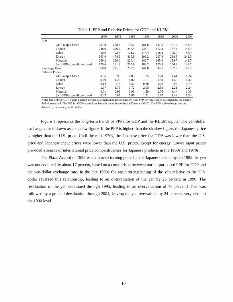
Table 1: PPP and Relative Prices for GDP and KLEM 1960 1973 1985 1990 1995 2000 2004

PPPGDP-output based 201.9 258.8 199.1 181.0 167.5 151.9 133.9Capital 248.9 326.2 242.4 233.1 172.3 157.4 143.9Labor 50.0 122.8 121.0 115.4 118.8 105.0 85.5Energy 563.9 478.8 410.9 296.2 267.8 238.6 242.5Material 256.2 269.0 220.4 186.7 165.4 154.7 143.7(ref)GDP-expenditure based 170.6 231.2 205.9 189.2 175.5 154.9 133.7

Exchange Rate 360.0 271.8 238.5 144.8 94.1 107.8 108.2Relative Prices

GDP-output based 0.56 0.95 0.83 1.25 1.78 1.41 1.24Capital 0.69 1.20 1.02 1.61 1.83 1.46 1.33Labor 0.14 0.45 0.51 0.80 1.26 0.97 0.79Energy 1.57 1.76 1.72 2.05 2.85 2.21 2.24Material 0.71 0.99 0.92 1.29 1.76 1.44 1.33(ref)GDP-expenditure based 0.47 0.85 0.86 1.31 1.87 1.44 1.24

Note: The PPP for GDP-output based is defined as a translog index of industry-level PPP for value added calculated by the double deflation method. The PPP for GDP-expenditure based is the estimates by the Eurostat-OECD. The PPP and exchange rate are defined by Japanese yen/ US dollar.

Figure 1 represents the long-term trends of PPPs for GDP and the KLEM inputs. The yen-dollar

exchange rate is drawn as a shadow figure. If the PPP is higher than the shadow figure, the Japanese price

is higher than the U.S. price. Until the mid-1970s, the Japanese price for GDP was lower than the U.S.

price and Japanese input prices were lower than the U.S. prices, except for energy. Lower input prices

provided a source of international price competitiveness for Japanese products in the 1960s and 1970s.

The Plaza Accord of 1985 was a crucial turning point for the Japanese economy. In 1985 the yen

was undervalued by about 17 percent, based on a comparison between our output-based PPP for GDP and

the yen-dollar exchange rate. In the late 1980s the rapid strengthening of the yen relative to the U.S.

dollar reversed this relationship, leading to an overvaluation of the yen by 25 percent in 1990. The

revaluation of the yen continued through 1995, leading to an overvaluation of 78 percent! This was

followed by a gradual devaluation through 2004, leaving the yen overvalued by 24 percent, very close to

the 1990 level.

11

0

100

200

300

400

500

600

1960 1965 1970 1975 1980 1985 1990 1995 2000 2005

Average Exchange Rate

PPP for GDP-output based

PPP for Capital Input

PPP for Labor Input

PPP for Energy Input

PPP for Material Input

(ref) PPP for GDP-expenditure based (OECD)

（Japanese Yen/US Dollar）

Figure 1: PPP for GDP and KLEM during 1960-2004

The Japanese economy spent more than a decade overcoming the huge overvaluation of the yen

that followed the Plaza Accord. This was accomplished mainly by domestic deflation, rather than

devaluation of the yen. The price of GDP in Japan, relative to the U.S., declined by four percent annually

through 2004 from the peak attained in 1994. The decline in the PPP for GDP at 2.5 percent per year was

the result of modest inflation in the US of 1.4 percent and deflation in Japan of 1.1 percent. In addition,

the yen-dollar exchange rate fell by 1.5 percent per year.

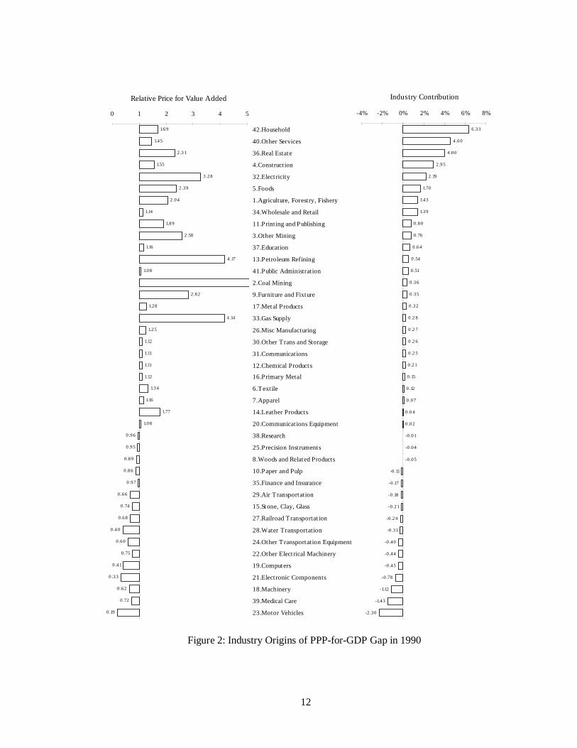
Figure 2 presents industry-level relative prices for value added and industry origins of the gap in

the PPP of 181.0 yen per dollar of the output-based GDP in 1990. The Japanese price for value added was

lower than the U.S. price in sixteen industries, while the Japanese price for gross output was lower in only

ten industries. Even if the relative price for gross output is greater than unity, the relative price for value

added can be less than unity as a consequence of high prices of energy and materials inputs in Japan. The

Household sector produces services of owner-occupied dwellings and consumer durables and made the

greatest contribution to the PPP for GDP in 1990. This reflects high prices of buildings and land in Japan

and the large share of value added by the Household sector. Electricity, which is very expensive in Japan,

pushed up the Japanese PPP by 2.2 percent.

12

-2 .30

-1.43

-1.12

-0 .78

-0 .45

-0 .44

-0 .40

-0 .31

-0 .24

-0 .21

-0 .18

-0 .17

-0 .11

-0 .05

-0 .04

-0 .01

0 .0 2

0 .0 4

0 .07

0 .12

0 .15

0 .21

0 .2 5

0 .2 6

0 .2 7

0 .2 8

0 .32

0 .35

0 .36

0 .51

0 .54

0 .64

0 .76

0 .80

1.39

1.43

1.70

2 .19

2 .95

4 .00

4 .60

6 .33

-4% -2% 0% 2% 4% 6% 8%

Industry Contribution

1.69

1.45

2 .3 1

1.55

3 .28

2 .39

2 .04

1.14

1.89

2 .58

1.16

4 .17

1.08

2 .82

1.28

4 .14

1.25

1.12

1.11

1.11

1.12

1.34

1.16

1.77

1.08

0 .96

0 .95

0 .89

0 .86

0 .97

0 .66

0 .74

0 .68

0 .4 0

0 .60

0 .75

0 .41

0 .33

0 .62

0 .72

0 .19

0 1 2 3 4 5

42.Household

40.Other Services

36.Real Estate

4.Construct ion

32.Elect ricity

5.Foods

1.Agriculture, Forest ry, Fishery

34.Wholesale and Retail

11.Print ing and Publishing

3.Other Mining

37.Education

13.Petroleum Refining

41.Public Administration

2.Coal Mining

9.Furniture and Fixture

17.Metal Products

33.Gas Supply

26.Misc Manufacturing

30.Other T rans and Storage

31.Communicat ions

12.Chemical Products

16.Primary Metal

6.Text ile

7.Apparel

14.Leather Products

20.Communicat ions Equipment

38.Research

25.Precision Inst ruments

8.Woods and Related Products

10.Paper and Pulp

35.Finance and Insurance

29.Air T ransportation

15.Stone, Clay, Glass

27.Railroad Transportat ion

28.Water Transportation

24.Other T ransportation Equipment

22.Other Elect rical Machinery

19.Computers

21.Elect ronic Components

18.Machinery

39.Medical Care

23.Motor Vehicles

Relative Price for Value Added

Figure 2: Industry Origins of PPP-for-GDP Gap in 1990

13

ii. Economic Growth in the U.S. and Japan

Table 2 summarizes our empirical results on economic growth and its sources for the U.S. and

Japanese economies. Despite the long economic recession in Japan, beginning in the early 1990s, rapid

technological progress in the IT-producing industries diffused quickly through investment in information

technology (IT) equipment and software by the IT-using industries. Jorgenson and Nomura (2005)13 have

discussed these findings through 2000 in greater detail. Table 2 shows that the trends they identified have

continued through 2004. Japanese economic growth slowed further after 2000, but the contribution of IT-

capital input continued to rise.

The annual rate of total factor productivity (TFP) growth in Japan improved from 0.48 percent per

year in 1995-2000 to 0.57 percent during 2000-2004. The contribution of labor input was negative in both

periods, but rose slightly from -0.19 to -0.15. The contribution of Non-IT-capital input in Japan dipped

substantially from 1995-2000 to 2000-2004, accounting for the slowdown in Japanese economic growth.

Despite this slowing trend, the contribution of investment in IT capital accelerated. The contribution of IT

to the growth of capital input expanded from 13.9 percent in 1990-1995 to 31.2 percent during 1995-2000,

and reached 51.6 percent for the period 2000-2004, considerably exceeding the U.S. contribution of 43.1

percent in that period.

Expanding labor input was an important source of U.S. economic growth during 1960-2000, but

this ended abruptly with the dot-com crash of 2000. Labor input declined at the rate of 0.17 percent per

year during 2000-2004. Another significant change in the U.S. economy after 2000 was the substantial

increase in the contribution of TFP growth and the shift in its industry origins. The annual growth rate of

TFP during 2000-2004 was 1.27 percent per year, close to twice the growth rate of the late 1990s and 2.7

times the long-term average growth rate during 1960-2000 of 0.46 percent.

13 We have extended the Japanese data used in Jorgenson and Nomura (2005) through 2004. In addition, we have revised the data after 1995 to incorporate the Annual Report on National Accounts (Economic and Social Research Institute, Cabinet Office) published in May 2006. This report is the first to include the 2000 benchmark revision. Second, we have revised the imputed cost for owner-occupied housing. In the Japanese national accounts, the estimation method for the cost of owner-occupied housing was substantially improved in the 2000 benchmark. As a consequence, the imputed cost was reduced from 49.9 trillion yen in 2000, based on the 1995 benchmark, to 42.8 trillion. Third, we have revised the allocation of land for dwellings between the Household and the Real Estate industries, based on estimates by Hideyuki Mizobuchi. Finally, we have introduced new estimates for work-in-progress inventories for cultivated assets as a capital input, consistent with the recommendation of the 1993 SNA. The values for the inventory stock on cultivated assets estimated by Nomura are 3.3, 8.6, and 3.9 trillion yen at current prices as of the end of 1960, 1980, and 2000, respectively.

14

Table 2: Sources of Economic Growth in the U.S. and Japan 1960-73 1973-90 1990-95 95-2000 2000-04 1960-2004

Value Added 3.90 2.83 2.35 4.12 2.56 3.21Capital Input 1.81 1.59 1.19 2.14 1.46 1.66

IT Capital 0.21 0.41 0.49 0.97 0.63 0.44Non-IT Capital 1.60 1.18 0.70 1.16 0.83 1.22

Labor Input 1.29 1.08 0.81 1.29 -0.17 1.02Total Factor Productivity 0.81 0.17 0.35 0.69 1.27 0.54

Agriculture 0.00 0.13 0.03 0.07 0.10 0.07IT-manufacturing 0.09 0.20 0.27 0.48 0.04 0.19Motor Vehicle 0.02 0.00 -0.01 0.02 0.06 0.01Other manufacturing 0.52 -0.02 0.11 0.21 0.04 0.19Communications 0.01 0.06 -0.01 -0.04 0.07 0.03Trade 0.17 0.15 0.07 0.15 0.51 0.18Finance & Insurance -0.05 0.01 0.04 0.11 0.30 0.03Other services 0.04 -0.37 -0.14 -0.30 0.15 -0.17

Value Added 10.00 4.50 1.31 1.31 1.14 5.10Capital Input 4.95 2.19 1.93 1.02 0.72 2.71

IT Capital 0.22 0.26 0.27 0.32 0.37 0.27Non-IT Capital 4.72 1.93 1.66 0.70 0.35 2.44

Labor Input 1.75 1.12 -0.16 -0.19 -0.15 0.90Total Factor Productivity 3.30 1.18 -0.46 0.48 0.57 1.48

Agriculture 0.20 0.00 0.06 -0.01 -0.04 0.06IT-manufacturing 0.17 0.21 0.09 0.42 0.35 0.22Motor Vehicle 0.28 0.13 0.00 0.02 0.11 0.14Other manufacturing 1.78 0.41 -0.33 0.17 0.08 0.68Communications 0.07 0.05 0.07 0.12 0.08 0.07Trade 0.94 0.28 0.01 -0.13 -0.03 0.37Finance & Insurance 0.23 0.10 -0.22 0.15 0.04 0.10Other services -0.36 0.01 -0.14 -0.26 -0.03 -0.15

United States

Japan

Note: All figures are average annual growth rates.Value added is aggregated from industry GDPs evaluated at the factor cost.

Perhaps surprisingly, the substantial improvement in U.S. TFP growth between 1995-2000 and

2000-2004 was achieved by a wide variety of IT-using industries rather than the IT-producing sectors as

discussed more in detail in Jorgenson, Ho, Samuels, and Stiroh (2007). The TFP contribution by the IT-

manufacturing sector was only 0.04 percent, a precipitous drop from 0.48 percent during 1995-2000. By

contrast the TFP contributions in communications, trade, and finance and insurance improved by 0.11,

0.36, and 0.19 percent points, respectively. Also, the negative contribution of -0.30 percent per year in

other services during the late 1990s gave way to a positive 0.15 percent after 2000.

15

0 .07

-0 .51

-1.86

0 .64

-0 .61

1.25

-1.62

1.76

-2 .20

0 .28

0 .93

4 .67

-3 .03

-1.00

-0 .04

0 .53

-0 .34

-0 .55

0 .00

0 .00

0 .00

-1.29

0 .45

0 .06

-0 .69

0 .37

0 .22

-0 .93

0 .41

-0 .14

0 .79

-0 .71

0 .28

-0 .63

-2 .62

-1.57

1.35

-0 .09

0 .06

6 .56

-4 .17

-4 .49

-5% 0% 5% 10%

Japan

2 .06

1.95

1.66

1.61

1.4 0

1.16

1.08

0 .96

0 .95

0 .80

0 .74

0 .50

0 .43

0 .33

0 .30

0 .08

0 .06

0 .04

0 .00

0 .00

-0 .05

-0 .13

-0 .16

-0 .27

-0 .37

-0 .49

-0 .80

-0 .91

-0 .93

-0 .96

-1.23

-1.24

-1.29

-2 .09

-2 .09

-2 .97

-3 .04

-3 .33

-4 .37

-11.69

-16 .06

5.01

-20% -15% -10% -5% 0% 5%



31.Communicat ions


40.Other Services




3.Other Mining

18.Machinery

23.Motor Vehicles

39.Medical Care

36.Real Estate






37.Educat ion

42.Household


6.Textile



10.Paper and Pulp


7.Apparel

38.Research

4.Const ruct ion


5.Foods

17.Metal Products

2.Coal Mining


13.Pet roleum Refining


16.Primary Metal

32.Elect ricity

33.Gas Supply

14.Leather Products

19.Computers


United States

Figure 3: Changes in Growth of Industry TFP: 2000-2004 less 1995-2000

16

-0 .18

0 .11

-0 .11

-0 .03

0 .41

0 .00

-0 .20

0 .00

0 .09

0 .08

-0 .03

0 .02

-0 .01

0 .03

0 .00

0 .01

-0 .02

0 .00

0 .00

0 .00

0 .01

0 .00

0 .00

0 .00

-0 .01

0 .00

0 .00

-0 .01

-0 .01

0 .00

0 .01

0 .01

-0 .04

0 .00

-0 .02

-0 .09

0 .06

-0 .06

0 .05

0 .07

0 .07

-0 .11

-0.4 -0.2 0.0 0.2 0.4 0.6

Japan

0 .4 5

0 .36

0 .19

0 .11

0 .0 8

0 .07

0 .05

0 .0 4

0 .0 4

0 .0 4

0 .03

0 .03

0 .0 2

0 .02

0 .01

0 .01

0 .00

0 .00

0 .00

0 .00

0 .00

0 .00

0 .00

0 .00

0 .00

0 .00

0 .00

-0 .01

-0 .01

-0 .01

-0 .01

-0 .01

-0 .02

-0 .02

-0 .03

-0 .06

-0 .06

-0 .08

-0 .09

-0 .14

-0 .17

-0 .25

-0.3 -0.2 -0.1 0.0 0.1 0.2 0.3 0.4 0.5

40.Other Services



31.Communicat ions

39.Medical Care


36.Real Estate


23.Motor Vehicles



18.Machinery

3.Other Mining







38.Research


42.Household


37.Education

6.Text ile

2.Coal Mining

14.Leather Products

10.Paper and Pulp


7.Apparel




33.Gas Supply

17.Metal Products

16.Primary Metal

5.Foods

13.Petroleum Refining

32.Elect ricity

4.Construct ion

19.Computers


United States

Figure 4: Changes in Contribution of Industry TFP to Economic Growth: 2000-2004 less 1995-2000

17

Figures 3 and 4 compare industry-level TFP growth and contributions to economic growth

between the periods 1995-2000 and 2000-2004. In the key IT-producing sectors, Electronic Components

and Computers, TFP growth in the U.S. slowed by more than ten percentage points. The improvement of

TFP growth in the IT-using sectors seems modest by comparison with improvements of 1.9 percentage

points in Communications, 1.7 in Wholesale and Retail Trade, 1.6 points in Other Services, and 1.2 points

in Finance and Insurance. However, as shown in Figure 4, these industries made substantially increased

contributions to the U.S. economic growth, reflecting their large Domar weights, as presented in Equation

(24) of the Methodological Appendix.

The resurgence of U.S. economic growth during 1995-2000 was powered by an acceleration of

TFP growth in the IT-producing industries and a resulting surge of investment in IT capital by the IT-

using sectors. After 2000 productivity growth plummeted in the IT-producing sectors, but greatly

accelerated in the IT-using industries. The end of the investment boom of the late 1990s with the dot-com

crash of 2000 resulted in a substantial fall in the contributions of investment in IT- and non-IT-capital

inputs after 2000. The growth of labor input plunged by two full percentage points!

There was no resurgence of Japanese economic growth during 1995-2000; however, the

contribution of TFP revived during this period and rose further during 2000-2004. The contribution of

TFP in IT-manufacturing in Japan rose from 0.09 per year in 1990-1995 to 0.42 percent during 1995-

2000, before receding to 0.35 percent after 2000, well above the U.S. contribution of 0.04 percent. The

contribution of investment in IT-capital input rose steadily from 0.27 percent per year in 1990-1995 to

0.32 percent in 1995-2000 and 0.37 percent after 2000.

iii. Level Comparisons of Output, Input, and Productivity

Table 3 summarizes the productivity gap between the U.S. and Japan. This table compares

relative levels of output, output per capita, input per capita, and total factor productivity between the two

economies over the period 1960-2004. Differences in output per capita can be decomposed into

differences in input per capita and TFP, the ratio of output to input. For example, Japanese GDP was 30.2

percent of the U.S. level in 2004. GDP per capita in Japan was 69.5 percent of U.S. GDP per capita, while

Japanese input per capita was 87.6 percent and Japanese TFP was 79.5 percent of the corresponding U.S.

levels.

18

Table 3: Relative Levels of Output, Input, and Total Factor Productivity 1960 1973 1980 1990 1995 2000 2004

Output 13.2 29.2 32.7 38.7 36.8 32.0 30.2Output per Capita 25.5 56.7 63.6 78.3 78.0 71.2 69.5Input per Capita 48.9 78.4 84.5 91.2 94.6 87.2 87.6Total Factor Productivity 52.4 72.5 75.4 86.1 82.6 81.7 79.5Note: All figures present the relative values (Japan/U.S.) in each period.

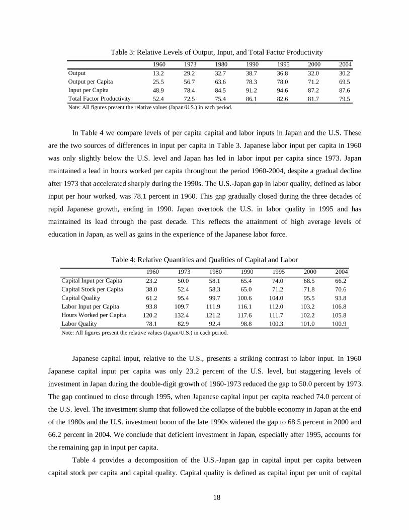
In Table 4 we compare levels of per capita capital and labor inputs in Japan and the U.S. These

are the two sources of differences in input per capita in Table 3. Japanese labor input per capita in 1960

was only slightly below the U.S. level and Japan has led in labor input per capita since 1973. Japan

maintained a lead in hours worked per capita throughout the period 1960-2004, despite a gradual decline

after 1973 that accelerated sharply during the 1990s. The U.S.-Japan gap in labor quality, defined as labor

input per hour worked, was 78.1 percent in 1960. This gap gradually closed during the three decades of

rapid Japanese growth, ending in 1990. Japan overtook the U.S. in labor quality in 1995 and has

maintained its lead through the past decade. This reflects the attainment of high average levels of

education in Japan, as well as gains in the experience of the Japanese labor force.

Table 4: Relative Quantities and Qualities of Capital and Labor 1960 1973 1980 1990 1995 2000 2004

Capital Input per Capita 23.2 50.0 58.1 65.4 74.0 68.5 66.2Capital Stock per Capita 38.0 52.4 58.3 65.0 71.2 71.8 70.6Capital Quality 61.2 95.4 99.7 100.6 104.0 95.5 93.8Labor Input per Capita 93.8 109.7 111.9 116.1 112.0 103.2 106.8Hours Worked per Capita 120.2 132.4 121.2 117.6 111.7 102.2 105.8Labor Quality 78.1 82.9 92.4 98.8 100.3 101.0 100.9Note: All figures present the relative values (Japan/U.S.) in each period.

Japanese capital input, relative to the U.S., presents a striking contrast to labor input. In 1960

Japanese capital input per capita was only 23.2 percent of the U.S. level, but staggering levels of

investment in Japan during the double-digit growth of 1960-1973 reduced the gap to 50.0 percent by 1973.

The gap continued to close through 1995, when Japanese capital input per capita reached 74.0 percent of

the U.S. level. The investment slump that followed the collapse of the bubble economy in Japan at the end

of the 1980s and the U.S. investment boom of the late 1990s widened the gap to 68.5 percent in 2000 and

66.2 percent in 2004. We conclude that deficient investment in Japan, especially after 1995, accounts for

the remaining gap in input per capita.

Table 4 provides a decomposition of the U.S.-Japan gap in capital input per capita between

capital stock per capita and capital quality. Capital quality is defined as capital input per unit of capital

19

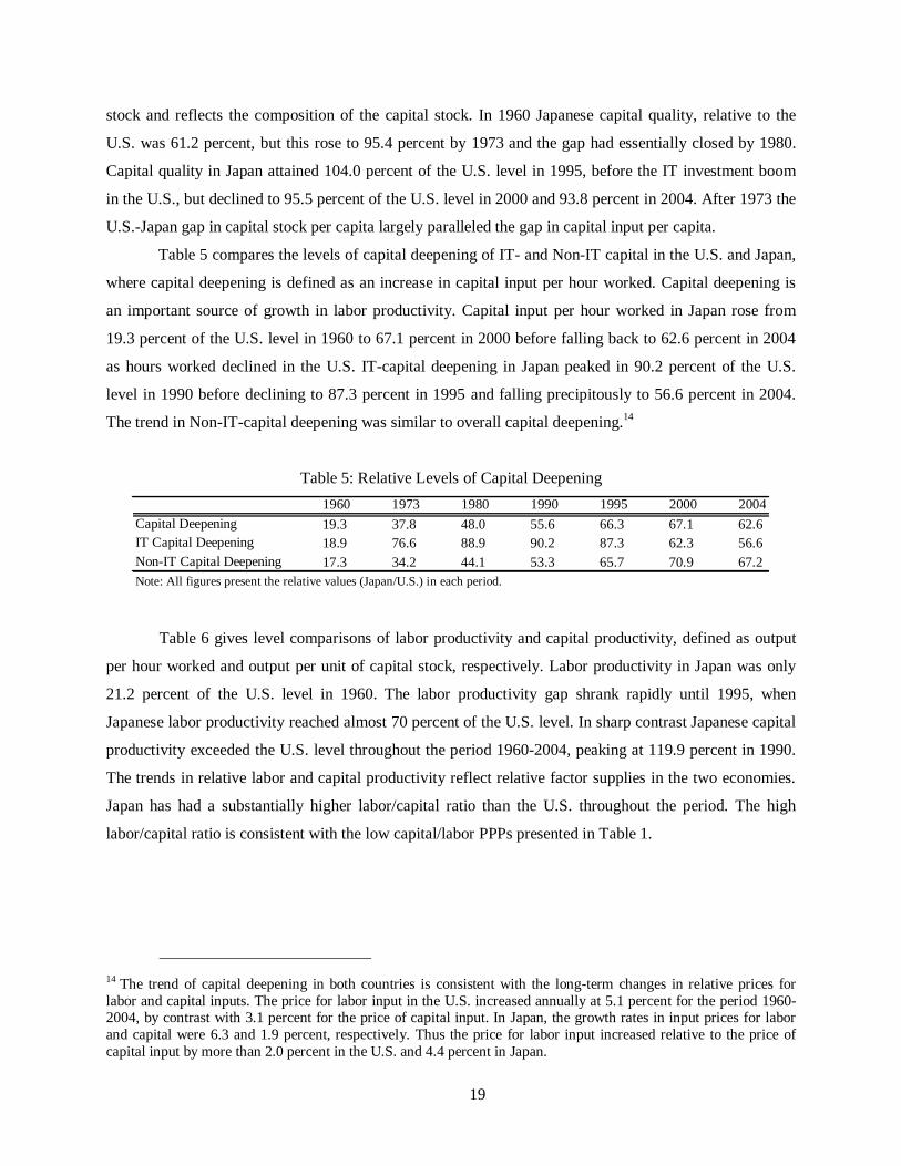
stock and reflects the composition of the capital stock. In 1960 Japanese capital quality, relative to the

U.S. was 61.2 percent, but this rose to 95.4 percent by 1973 and the gap had essentially closed by 1980.

Capital quality in Japan attained 104.0 percent of the U.S. level in 1995, before the IT investment boom

in the U.S., but declined to 95.5 percent of the U.S. level in 2000 and 93.8 percent in 2004. After 1973 the

U.S.-Japan gap in capital stock per capita largely paralleled the gap in capital input per capita.

Table 5 compares the levels of capital deepening of IT- and Non-IT capital in the U.S. and Japan,

where capital deepening is defined as an increase in capital input per hour worked. Capital deepening is

an important source of growth in labor productivity. Capital input per hour worked in Japan rose from

19.3 percent of the U.S. level in 1960 to 67.1 percent in 2000 before falling back to 62.6 percent in 2004

as hours worked declined in the U.S. IT-capital deepening in Japan peaked in 90.2 percent of the U.S.

level in 1990 before declining to 87.3 percent in 1995 and falling precipitously to 56.6 percent in 2004.

The trend in Non-IT-capital deepening was similar to overall capital deepening.14

Table 5: Relative Levels of Capital Deepening 1960 1973 1980 1990 1995 2000 2004

Capital Deepening 19.3 37.8 48.0 55.6 66.3 67.1 62.6IT Capital Deepening 18.9 76.6 88.9 90.2 87.3 62.3 56.6Non-IT Capital Deepening 17.3 34.2 44.1 53.3 65.7 70.9 67.2Note: All figures present the relative values (Japan/U.S.) in each period.

Table 6 gives level comparisons of labor productivity and capital productivity, defined as output

per hour worked and output per unit of capital stock, respectively. Labor productivity in Japan was only

21.2 percent of the U.S. level in 1960. The labor productivity gap shrank rapidly until 1995, when

Japanese labor productivity reached almost 70 percent of the U.S. level. In sharp contrast Japanese capital

productivity exceeded the U.S. level throughout the period 1960-2004, peaking at 119.9 percent in 1990.

The trends in relative labor and capital productivity reflect relative factor supplies in the two economies.

Japan has had a substantially higher labor/capital ratio than the U.S. throughout the period. The high

labor/capital ratio is consistent with the low capital/labor PPPs presented in Table 1.

14 The trend of capital deepening in both countries is consistent with the long-term changes in relative prices for labor and capital inputs. The price for labor input in the U.S. increased annually at 5.1 percent for the period 1960-2004, by contrast with 3.1 percent for the price of capital input. In Japan, the growth rates in input prices for labor and capital were 6.3 and 1.9 percent, respectively. Thus the price for labor input increased relative to the price of capital input by more than 2.0 percent in the U.S. and 4.4 percent in Japan.

20

Table 6: Relative Levels of Labor Productivity and Capital Productivity 1960 1973 1980 1990 1995 2000 2004

Labor Productivity 21.2 42.8 52.5 66.6 69.9 69.7 65.7Capital Productivity 109.8 113.2 109.4 119.9 105.4 103.9 104.9Note: All figures present the relative values (Japan/U.S.) in each period.

The sources of U.S.-Japan labor productivity gap are shown in Figure 5. The y-axis gives the

logarithm of the relative productivity level. In 1960 lower Non-IT-capital deepening in Japan explained

50.1 percent of the U.S.-Japan labor productivity gap, while lower Japanese TFP explained 40.4 percent.

The lower quality of labor input and lower IT-capital deepening contributed 8.8 percent and 0.7 percent,

respectively. As a consequence of rapid capital deepening in Japan, the TFP gap has been the major

source of lower labor productivity since the mid-1990s. Lower TFP explains 57.0 percent of the labor

productivity gap in 2004, while Non-IT-capital deepening accounts for 37.3 percent.

-1.6

-1.4

-1.2

-1.0

-0.8

-0.6

-0.4

-0.2

0.0

1960 1965 1970 1975 1980 1985 1990 1995 2000

IT Capital Deepening Non-IT Capital DeepeningLabor Quality TFP

Labor Productivity Gap

log (relative productivity level: Japan/US)

Figure 5: Sources of U.S.-Japan Labor Productivity Gap

iv. Industry Origins of the U.S.-Japan Productivity Gap

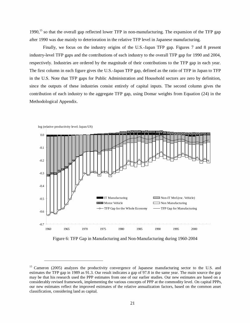
Figure 6 presents long-term trends of TFP gaps in manufacturing and non-manufacturing sectors.

In 1960 both gaps were very large. However, the TFP gap for manufacturing had almost disappeared by

21

1990,15 so that the overall gap reflected lower TFP in non-manufacturing. The expansion of the TFP gap

after 1990 was due mainly to deterioration in the relative TFP level in Japanese manufacturing.

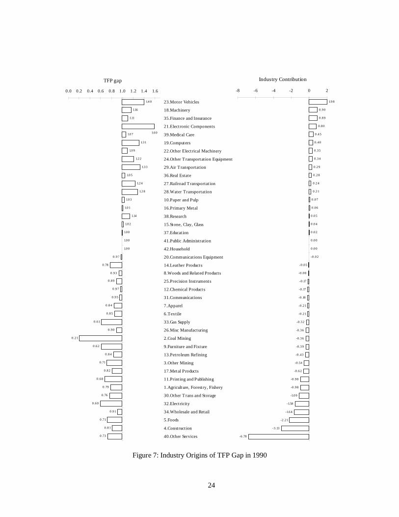
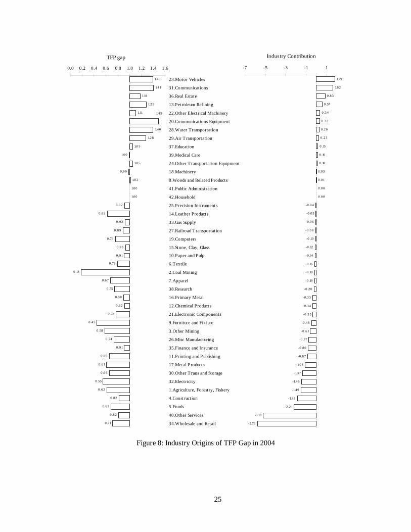
Finally, we focus on the industry origins of the U.S.-Japan TFP gap. Figures 7 and 8 present

industry-level TFP gaps and the contributions of each industry to the overall TFP gap for 1990 and 2004,

respectively. Industries are ordered by the magnitude of their contributions to the TFP gap in each year.

The first column in each figure gives the U.S.-Japan TFP gap, defined as the ratio of TFP in Japan to TFP

in the U.S. Note that TFP gaps for Public Administration and Household sectors are zero by definition,

since the outputs of these industries consist entirely of capital inputs. The second column gives the

contribution of each industry to the aggregate TFP gap, using Domar weights from Equation (24) in the

Methodological Appendix.

-0.7

-0.6

-0.5

-0.4

-0.3

-0.2

-0.1

0.0

1960 1965 1970 1975 1980 1985 1990 1995 2000

IT Manufacturing Non-IT Mnf.(exc. Vehicle)Motor Vehicle Non Manufacturing

TFP Gap for the Whole Economy TFP Gap for Manufacturing

log (relative productivity level: Japan/US)

Figure 6: TFP Gap in Manufacturing and Non-Manufacturing during 1960-2004

15 Cameron (2005) analyzes the productivity convergence of Japanese manufacturing sector to the U.S. and estimates the TFP gap in 1989 as 91.3. Our result indicates a gap of 97.8 in the same year. The main source the gap may be that his research used the PPP estimates from one of our earlier studies. Our new estimates are based on a considerably revised framework, implementing the various concepts of PPP at the commodity level. On capital PPPs, our new estimates reflect the improved estimates of the relative annualization factors, based on the common asset classification, considering land as capital.

22

In 1990 the U.S.-Japan productivity gap reached a minimum for the period 1960-2004. Japanese

TFP exceeded that in the U.S. for 17 of 40 industries, led by Motor Vehicles. Substantial positive

contributions to Japanese TFP, relative to the U.S., were also made by Machinery, Finance and Insurance,

and Electronic Components. Other Services accounted for nearly half of the overall TFP gap in 1990.

Construction, Foods, Wholesale and Retail Trade and Electricity, all domestically oriented industries in

Japan, also made sizable contributions to the overall TFP gap in 1990.

In 2004 Motor Vehicles continued to make the largest contributions to Japanese TFP, relative to

the U.S. Communications and Real Estate emerged as major contributors. The lagging industries in 1990

retained their places at the bottom in 2004 with Agriculture, Forestry, and Fisheries. Wholesale and Retail

Trade and Other Services, two industries largely sheltered from international competition, account for

25.1 and 22.5 percent, respectively, of the lower TFP level of the Japanese economy.

Figure 9 depicts the long-term trends in TFP levels in the U.S. and Japan for twelve particularly

important industries. Productivity levels in each industry are normalized by the U.S. productivity level in

1960. In 1960 the TFP level in Agriculture, Forestry, and Fishery was only slightly inferior to the U.S.,

but the TFP gap widened after 1973, reflecting large differences in the scale of individual production

units, as well as massive public investments in new agricultural technology in the U.S. Construction

showed declining productivity trends in both economies with the U.S.-Japan TFP gap gradually closing.

We next consider three IT-producing sectors – Computers, Communications Equipment, and

Electronic Components. The Japanese computer industry led its U.S. counterpart until the early 1990s,

when U.S. TFP growth accelerated sharply. This was followed five years later by a similar acceleration in

Japanese TFP growth. The deceleration of TFP growth in the U.S. industry after 2000 has reduced, but

not eliminated, the U.S.-Japan gap. The Japanese telecommunications equipment industry achieved parity

with the U.S. industry in the late 1970s but underwent a substantial acceleration in the mid-1990s and

emerged with a sizable lead by 2004. The U.S. electronic components industry lagged behind the

Japanese industry until the mid-1990s, but gained a substantial lead in the late 1990s that has shrunk but

not entirely disappeared since the dot-com crash of 2000.

The U.S. started with an early lead in Other Electrical Machinery but the Japanese industry

achieved parity by 1973. Relative productivity levels have been very similar over the following three

decades with Japan emerging with a slight lead in 2004. The Japanese Motor Vehicles industry has led its

U.S. counterpart since the early 1970s. However, the TFP gap has been fairly constant since the 1980s.

The Japanese Communications industry first achieved parity with the U.S. industry around 1973, but

established a sizable lead beginning in the early 1990s. All three industries experienced substantial gains

in productivity throughout the period 1960-2004.

23

Finally, Wholesale and Retail Trade has contributed to the U.S. lead in overall TFP since 1960.

The TFP gap has widened dramatically since the end of the 1990s, due to a slump in TFP growth in Japan

and an acceleration of TFP growth in the U.S. The U.S. had a large productivity advantage over Japan in

Finance and Insurance in 1960, but this shrank dramatically from 1960-1973 and then more gradually

until the mid-1980s, when Japan emerged with an advantage for the first time. Both economies

experienced a sharp acceleration in TFP growth in this industry, beginning in the late 1990s. Other

Services has undergone a steady decline in TFP in both economies, but the U.S. has maintained an edge.

24

1.9 8

0 .90

0 .89

0 .80

0 .45

0 .40

0 .35

0 .34

0 .29

0 .28

0 .24

0 .21

0 .07

0 .06

0 .05

0 .04

0 .02

0 .00

0 .00

-0 .02

-0 .05

-0 .08

-0 .17

-0 .17

-0 .18

-0 .21

-0 .21

-0 .32

-0 .36

-0 .36

-0 .39

-0 .43

-0 .54

-0 .62

-0 .98

-0 .98

-1.09

-1.58

-1.64

-2 .21

-3 .13

-6 .78

-8 -6 -4 -2 0 2


1.4 0

1.16

1.11

1.07

1.31

1.09

1.22

1.33

1.05

1.24

1.28

1.03

1.01

1.14

1.02

1.00

1.00

1.00

0 .97

0 .78

0 .93

0 .89

0 .97

0 .95

0 .84

0 .85

0 .61

0 .90

0 .21

0 .62

0 .84

0 .71

0 .82

0 .68

0 .79

0 .76

0 .60

0 .91

0 .71

0 .81

0 .73

1.60

0.0 0.2 0.4 0.6 0.8 1.0 1.2 1.4 1.6

23.Motor Vehicles

18.Machinery



39.Medical Care

19.Computers




36.Real Estate



10.Paper and Pulp

16.Primary Metal

38.Research


37.Educat ion


42.Household


14.Leather Products




31.Communicat ions

7.Apparel

6.Textile

33.Gas Supply


2.Coal Mining



3.Other Mining

17.Metal Products




32.Elect ricity


5.Foods

4.Const ruct ion

40.Other Services

TFP gap

Figure 7: Industry Origins of TFP Gap in 1990

25

1.79

1.62

0 .83

0 .57

0 .34

0 .32

0 .26

0 .23

0 .15

0 .10

0 .10

0 .03

0 .01

0 .00

0 .00

-0 .04

-0 .05

-0 .06

-0 .08

-0 .10

-0 .12

-0 .14

-0 .16

-0 .18

-0 .19

-0 .20

-0 .33

-0 .34

-0 .35

-0 .48

-0 .61

-0 .77

-0 .80

-0 .87

-1.08

-1.37

-1.46

-1.49

-1.86

-2 .21

-5.18

-5.76

-7 -5 -3 -1 1


1.40

1.41

1.18

1.2 9

1.11

1.40

1.28

1.0 5

1.00

1.0 5

0 .99

1.0 2

1.00

1.00

0 .92

0 .63

0 .92

0 .89

0 .76

0 .93

0 .91

0 .79

0 .18

0 .67

0 .75

0 .90

0 .92

0 .78

0 .45

0 .58

0 .74

0 .91

0 .66

0 .61

0 .66

0 .55

0 .62

0 .82

0 .69

0 .82

0 .71

1.49

0.0 0.2 0.4 0.6 0.8 1.0 1.2 1.4 1.6

23.Motor Vehicles

31.Communicat ions

36.Real Estate






37.Educat ion

39.Medical Care


18.Machinery



42.Household


14.Leather Products

33.Gas Supply


19.Computers


10.Paper and Pulp

6.Textile

2.Coal Mining

7.Apparel

38.Research

16.Primary Metal




3.Other Mining




17.Metal Products


32.Elect ricity


4.Const ruct ion

5.Foods

40.Other Services


TFP gap

Figure 8: Industry Origins of TFP Gap in 2004

26

0.0

0.2

0.4

0.6

0.8

1.0

1.2

1.4

1.6

1.8

1960 1970 1980 1990 2000

23.M otor Vehicles

0.0

0.2

0.4

0.6

0.8

1.0

1.2

1.4

1.6

1.8

1960 1970 1980 1990 2000

34. Wholesale and Retail

0.0

0.2

0.4

0.6

0.8

1.0

1.2

1.4

1960 1970 1980 1990 2000

18.Machinery

0

5

10

15

20

25

30

35

1960 1970 1980 1990 2000

21. Electronic Components

0.0

0.5

1.0

1.5

2.0

2.5

1960 1970 1980 1990 2000

31.Communications

0.0

0.2

0.4

0.6

0.8

1.0

1.2

1960 1970 1980 1990 2000


01020304050

60708090

100

1960 1970 1980 1990 2000

19.Computers

0.00.20.40.60.81.01.21.41.61.82.0

1960 1970 1980 1990 2000

22. Other Electrical Machinery

0.0

0.2

0.4

0.6

0.8

1.0

1.2

1960 1970 1980 1990 2000

4.Construction

0.0

0.2

0.4

0.6

0.8

1.0

1.2

1.4

1.6

1.8

1960 1970 1980 1990 2000

40. Other Service

0.00.20.40.60.81.01.21.41.61.82.0

1960 1970 1980 1990 2000

1.Agriculture, Forestry, Fishery

(US)

(Japan)

(Productitivy Level in the U.S. in 1960=1.0)

0.0

0.5

1.0

1.5

2.0

2.5

1960 1970 1980 1990 2000

20.Communications Equipment

Figure 9: TFP Level Comparison in Selected Industries during 1960-2004

27

IV. Conclusion

A number of persistent differences between the U.S. and Japanese economies have emerged from

our international comparisons, including substantial gaps in total factor productivity, defined as output per

unit of input. Allocating the U.S.-Japan productivity gap to its origins at the level of individual industries

is the first step in formulating policies to reduce or eliminate this gap. Both input per capita and total

factor productivity are important sources of differences in output per capita between the U.S. and Japan.

Japan has led the U.S. in hours worked per capita throughout the period 1960-2004 and now leads in

labor quality, defined as labor input per hour worked, as well.

Capital input presents a sharp contrast with labor input in U.S.-Japan comparisons. Japan began

with a very low level of capital input per capita, relative to the U.S. in 1960, but made substantial

progress in closing the gap through 1995. At that point the Japanese economy was still suffering from the

aftereffects of the collapse of the bubble economy of the 1980s, while the U.S. was beginning a massive

investment boom in IT equipment and software. Japan has lost considerable ground in capital input per

capita, relative to the U.S., after 1995, eventually reverting to the relative levels of the mid-1980s.

Japan has overcome the impact of the very substantial over-valuation of the yen that followed the

Plaza Accord of 1985. However, this has required a decade of domestic deflation, accompanied by

depressed investment levels and, especially, by insufficient investment in IT equipment and software.

Japanese TFP growth has revived, but continues to lag behind the U.S. Japan has been very successful in

exploiting new information technology in Communications equipment and Communications services. The

impressive rebound of TFP growth in the Japanese Computer and Electronic components industries will

continue to stimulate high levels of investment in information technology equipment and software by IT-

using industries in Japan.

Finally, Japan succeeded in raising its relative level of TFP from 52.4 percent of the U.S. level in

1960 to 86.1 percent in 1990. At that point seventeen of the 40 industries included in our U.S.-Japan

comparisons had higher levels of TFP in Japan and the Japanese manufacturing sector as a whole had

achieved parity with its U.S. counterpart. Japan’s TFP growth stalled during the decade 1990-2000. U.S.

TFP increased rapidly during the period 1995-2000 and then accelerated sharply from 2000-2004, as

Japan’s TFP growth began to revive. By 2004 only twelve Japanese industries had higher TFP than their

U.S. counterparts. Wholesale and Retail Trade and Other Services, two industries largely sheltered from

international competition, stand out as opportunities for substantial improvement in Japanese TFP,

relative to the U.S.

28

Methodological Appendix

i. Relative Price, Quantity, and Quality

(a) Elementary Level

We start with the definition of value, price, and quantity for output and inputs of capital, labor,

energy, and materials (K,L,E,M) at the elementary level. The nominal value cijtV ,q of industry j in country

c, evaluated by own-currency unit in each country, is defined as follows:

(3) cijt

cijt

cijt

cijt

cijt XPXPV ,,,,, ˆˆ qqqqq == ,

where cijtP ,q is the price index ( 0.1, =c

ijTPq as of a base year T) and cijtX ,q is the quantity index. The suffix

i represents a subscript for the elementary components in each category ),,,,( MELKY=q . For

example, in the case of labor input ( L=q ), the subscript i stands for categories cross-classified by sex,

age, education, and class of worker. Although the categories are different for each q , we use the same

subscript for simplicity.16 In comparing economies the industry classification j and elementary categories

i are assumed to be identical, reflecting the common classifications we have established for the U.S. and

Japan.

The last term in Equation (3) defines measures of price and quantity, cijtP ,ˆ q and c

ijtX ,ˆ q , which are

based on the same units in each economy. To clarify this we define the elementary quality cijQ ,q from the

quantities and prices as follows:

(4) cijt

cij

cijt XQX ,,, ˆ qqq = ,

(5) cijt

cij

cijt PQP ,,,ˆ qqq = .

At the elementary level the quality cijQ ,q represents a base-year unit price with constant quality between

the two economies, evaluated in terms of the currency units in each economy. This can be defined as the

quantity purchased by one unit of the currency of the base economy in a base year. For example, let the

U.S. be the base economy and “one-dollar’s worth” be the quantity unit, equivalent to the base-year value

of one dollar in the U.S. This provides the physical unit for each element of i applied to both economies.

The cost of purchasing one-dollar’s worth in each economy provides the unit price, cijtP ,ˆ q . Although the

quantity, cijtX ,q , is not directly comparable between the two economies, the quality-adjusted quantity, c

ijtX ,ˆ q ,

29

provides a comparable quantity measure. Also, cijtP ,ˆ q and c

ijQ ,q provide comparable measures of the

quality-adjusted unit price and quality with taking the exchange rates between currencies into account.17

For bilateral comparisons between the U.S. (c=U) and Japan (c=J), we define the quality-

adjusted quantity and price in Japan, using the U.S. quality for each element i. Equations (3)-(5) in Japan

are redefined as follows:

(6) Jijt

UJijt

UJijt

UJijt

UJijt XPXPV ,|,|,|,|, ˆˆ qqqqq == ,

(7) Jijt

Uij

UJijt XQX ,,|, ˆ qqq = ,

(8) UJijt

Uij

UJijt PQP |,,|,ˆ qqq = ,

where tJ

ijtUJ

ijt eVV ,|, qq = and tJ

ijtUJ

ijt ePP ,|, ˆˆ qq = , using the annual average exchange rate te (Japanese

yen per U.S. dollar). Equation (7) represents the quality-adjusted quantity measure in Japan, UJijtX |,q ,

which is directly comparable to the U.S. quantity measure, UijtX ,q , applying U.S. quality U

ijQ ,q . Equation

(8) represents the quality-adjusted price measure in Japan, UJijtP |,q , which is comparable to the U.S. price

index, UijtP ,q , adjusting for the US-Japan differences in quality and the exchange rate.

We define relative indexes for value, price, quantity, and quality between the U.S. and Japan as:

(9) Uijt

UJijt

ijt VV

RV ,

|,

q

qq = , U

ijt

UJijt

ijt PP

RP ,

|,

q

qq = ,

Uijt

UJijt

ijt PP

PR,

|,

ˆ

ˆˆ

q

qq = ,

Uijt

UJijt

ijt XX

RX ,

|,

q

qq = ,

Uijt

Jijt

ijt XX

XR,

,

ˆ

ˆˆ

q

qq = , U

ij

UJij

ij QQ

RQ ,

|,

q

qq = ,

where TJ

ijUJ

ij eQQ ,|, qq = , using the base-year exchange rate. At the elementary level the two measures

for relative price and quantity coincide, qqijtijt PRRP ˆ= and qq

ijtijt XRRX ˆ= , and the relative quality, qijRQ ,

is constant over time periods. The relative value, qijtRV , is identical with qq

ijtijt RXRP and qqijtijt XRPR ˆˆ .

The purchasing power parities for output and KLEM inputs at the elementary level are defined as

follows:

16 As described in Section II, the number of elementary categories, commonly defined for the U.S. and Japan, is 33 for capital inputs (K), 1596 for labor inputs (L), and 164 for intermediate inputs (E, M). 17 If we use one-dollar’s worth as an unit of quantity, then quality in the U.S., U

ijQ ,q , is identical to one for all i of

q . In the case of labor input, we assume hours worked provide an appropriate unit for one-dollar’s worth for labor

30

(10) U

ijt

Jijt

ijttijt PP

RPePPP,

,

ˆ

ˆq

qqq == .

Although the relative price depends on the exchange rate, the purchasing power parity (PPP) is

independent of it. The PPP can be interpreted as the relative cost of purchasing the one-dollar’s worth in

each economy. If qijtPPP in each category MELKY ,,,,=q is less than the exchange rate, that is, its

bilateral relative price, qijtRP , is less than one, the price in Japan is lower than the price in the U.S. As of

the base year T, the relative price coincides with the relative quality at the elementary level, qqijijT RQRP = .

Thus the quality-adjusted quantity measure in Japan in Equation (7) is measured using the base-year PPP:

(11) q

qq

ijT

JijtUJ

ijt PPPX

X,

|, = .

(b) Industry Level

We move to the industry-level formulation by aggregating elementary components. The value c

jtV ,q in j is described as the sum of elementary categories in MELKY ,,,,=q , evaluated in the

currency of each economy:

(12) å===i

cijt

cijt

cjt

cjt

cjt

cjt

cjt XPXPXPV ,,,,,,, ˆˆ qqqqqqq .

For output and KLEM inputs the industry-level translog quantity cjtX ,q and unweighted-sum c

jtX ,ˆ q are

defined as:

(13) cijt

i

cijt

cjt XvX ,,, lnln qqq D=D å ,

(14) å=i

cijt

cjt XX ,, ˆˆ qq ,

where the weights cijtv ,q are the two-period average shares of the elementary components in the nominal

value for each economy. For the base-year T the translog quantity index, cjTX ,q , is set equal to c

jTV ,q .

Next, to define comparable measures between the two economies at the industry level, we define

bilateral relative measures for price, quantity, and quality. The industry-level PPP for each q is assumed

to be a translog index of the elementary level PPPs, as follows:

(15) åºi

ijtijtjt PPPwPPP qqq lnln ,

input at the elementary level, as described later; then quality is defined by base-year labor compensation per hour

31

where the weights qijtw are the two-country average shares of the elementary components in the nominal

value for each q . The industry-level relative price is defined as tjtjt ePPPRP qq = . Using the base-year

industry-level PPP, we define quantity in Japan, UJjtX |,q , which is comparable to the U.S. industry-level

quantity, UjtX ,q , as follows:

(16) q

qq

jT

JjtUJ

jt PPPX

X,

|, = .

Using the quantity index, UJjtX |,q , we redefine the nominal value in Equation (12) and the

industry-level quality measure in Japan as follows:

(17) Jjt

UJjt

UJjt

UJjt

UJjt XPXPV ,|,|,|,|, ˆˆ qqqqq == ,

(18) Jjt

UJjt

UJjt XQX ,|,|, ˆ qqq = ,

(19) UJjt

UJjt

UJjt PQP |,|,|,ˆ qqq = ,

where tJ

jtUJ

jt eVV ,|, qq = .

The two measures of price in Japan, UJjtP |,q and UJ

jtP |,ˆ q , are comparable to the U.S. industry-level

prices, UjtP ,q and U

jtP ,ˆ q , respectively. These measures are defined in Equation (19) to be consistent with

the corresponding quantities, UJjtX |,q in (16) and J

jtX ,ˆ q in (14), respectively. Equations (18) and (19)

provide the industry-level quality index in Japan, UJjtQ |,q , which is comparable to the U.S. quality,

UjtQ ,q .18 The elementary-level quality defined in Equations (7) and (8) is constant over periods, but the

industry-level quality can change because of changes in composition.

At the industry level relative indexes for value, price, quantity, and quality between the U.S. and

Japan are defined as follows:

evaluated in the currency of each economy. 18 The Japan’s quality, UJ

jtQ |,q , is also written as qqjT

Jjt PPPQ , , where J

jtQ ,q is defined by Jjt

Jjt XX ,, ˆ qq . If we

define one-dollar’s worth for all i as a unit of quantity, the U.S. industry-level quality in the U.S., UjTQ ,q , is identical

to one in the base year T.

32

(20) Ujt

UJjt

jt VV

RV ,

|,

q

qq = , U

jt

UJjt

jt PP

RP ,

|,

q

qq = ,

Ujt

UJjt

jt PP

PR,

|,

ˆ

ˆˆ

q

qq = ,

Ujt

UJjt

jt XX

RX ,

|,

q

qq = ,

Ujt

Jjt

jt XX

XR,

,

ˆ

ˆˆ

q

qq = , U

jt

UJjt

jt QQ

RQ ,

|,

q

qq = ,

The relative value qjtRV is identical to qq

jtjt RXRP and qqjtjt XRPR ˆˆ . The two elementary-level measures for

price and quantity coincide as qqijtijt PRRP ˆ= and qq

ijtijt XRRX ˆ= , but the two measures for industry-level

relative price and quantity are not identical. They are written as:

(21) qqqjtjtjt XRRQRX ˆ= ,

(22) qqqjtjtjt RPRQPR =ˆ .

Only in the special case of equal PPPs across all elementary categories in each q , the relative quality qjtRQ is unity and the two measures for industry-level relative price and quantity coincide.

ii. Relative Productivity

Finally, we formulate the productivity gap, using relative quantities in Equation (20). Under the

assumptions of constant returns to scale and competitive markets in both countries, the relative measure

of total factor productivity (TFP) between the U.S. and Japan is defined as a translog index:

(23) Yjtjt

KLEMjtjt

KLEMjt

Yjtjt RPRPwRXwRXRT lnlnlnln -=-º åå

==

q

q

qq

q

q ,

where the weights, qjtw , are the average, two-country shares of KLEM inputs in the value of output,

which is assumed to be equal to the total compensation for all four KLEM inputs. The key to defining the

productivity gap is the base-year PPPs for output and the KLEM inputs, defined in Equation (16). We define the aggregate TFP gap as the Domar-weighted industry-level TFP gap:

(24) jtj

jtt RTdRT åº ln ,

where jtd weights are the average, two-country shares of the Domar weights. These weights multiply

industry productivity growth by the share of industry value added in GDP and divide by the share of

industry value added in industry output. These weights capture the relative importance of the industry in

33

GDP and the relative importance of value added in the industry’s output.19 Equation (24) provides the

framework for quantifying the industry origins of the productivity gap between the U.S. and Japan.

References

Ark, Bart van and Dirk Pilat (1993) “Productivity Levels in Germany, Japan, and the United States* Differences and Causes,” Brookings Papers on Economic Activity, Microeconomics, 1-48.

Cameron, Gavin (2005), “The Sun Also Rises: Productivity Convergence Between Japan and the USA, Journal of Economic Growth, 10, 387-408.

Inklaar, Robert and Marcel P. Timmer (2007), “International Comparisons of Industry Output, Inputs, and Productivity Levels: Methodology and New Results,” Economic Systems Research, this issue.

Jorgenson, Dale W., Mun S. Ho, and Kevin J. Stiroh (2005). Information Technology and the American Growth Resurgence, Cambridge, The MIT Press.

Jorgenson, Dale W., Mun S. Ho, Jon D. Samuels, and Kevin J. Stiroh (2007), “Industry Origins of the American Growth Resurgence,” Economic Systems Research, this issue.

Jorgenson, Dale W., and Masahiro Kuroda (1990). “Productivity and International Competitiveness in Japan and the United States, 1960-1985,” in C.R. Hulten, eds., Productivity Growth in Japan and the United States, University of Chicago Press, 29-55.

Jorgenson, Dale W., Masahiro Kuroda, and Mieko Nishimizu (1987), “Japan-U.S. Industry-Level Productivity Comparison, 1960-1979,” Journal of the Japanese and International Economies, 1, 1-30.

Jorgenson, Dale W., and Koji Nomura (2005). “The Industry Origins of Japanese Economic Growth,” Journal of the Japanese and International Economies, 19, 482-542.

Kuroda, Masahiro and Koji Nomura (1999). “Productivity Comparison and International Competitiveness,” Journal of Applied Input-Output Analysis, 5, 1-37.

Nomura, Koji (2004). Measurement of Capital and Productivity in Japan, Tokyo, Keio University Press, (in Japanese).

Nomura, Koji and Kozo Miyagawa (1999). “Measurement of US-Japan Relative Prices of Commodities,” Keizai Tokei Kenkyu (Research on Economic Statistics), Vol.27, No.3. (in Japanese).

Nomura, Koji and Jon D. Samuels (2003). “Wage Differentials and Structure in the U.S. and Japan, 1960-2000: Purchasing Power Parities for Labor Input,” RCGW Discussion Paper, Development Bank of Japan.

19 For further discussion of Domar weights, see Jorgenson and Nomura (2005), Section V.

The Industry Origins of the US-Japan Productivity Gap...KEO Discussion Paper No. 105 The Industry...

Documents

Transcript of The Industry Origins of the US-Japan Productivity Gap...KEO Discussion Paper No. 105 The Industry...