The individual life cycle and economic growth: An essay … · The individual life cycle and...
31
The individual life cycle and economic growth: An essay on demographic macroeconomics * Ben J. Heijdra ♯ University of Groningen; IHS (Vienna); CESifo; Netspar Jochen O. Mierau ‡ University of Groningen; Netspar October 2010 Abstract We develop a demographic macroeconomic model that captures the salient life-cycle fea- tures at the individual level and, at the same time, allows us to pinpoint the main mech- anisms at play at the aggregate level. At the individual level the model features both age-dependent mortality and productivity and allows for less-than-perfect annuity mar- kets. At the aggregate level the model gives rise to single-sector endogenous growth and includes a Pay-As-You-Go pension system. We show that ageing generally promotes eco- nomic growth due to a strong savings response. Under a defined benefit system the growth effect is still positive but lower than under a defined contribution system. Surprisingly, we find that an increase in the retirement age dampens the economic growth expansion following a longevity shock. JEL codes: D52, D91, E10, J20. Keywords: Annuity markets, pensions, retirement, endogenous growth, overlapping gen- erations, demography. ∗ We thank Jan van Ours and Laurie Reijnders for helpful comments and remarks. This paper was written during the second author’s visit to the Department of Economics of the University of Washington. The department’s hospitality is gracefully acknowledged. ♯ Corresponding author. Faculty of Economics and Business, University of Groningen, P.O. Box 800, 9700 AV Groningen, The Netherlands. Phone: +31-50-363-7303, Fax: +31-50-363-7337, E-mail: [email protected]. ‡ Faculty of Economics and Business, University of Groningen, P.O. Box 800, 9700 AV Groningen, The Netherlands. Phone: +31-50-363-8534, Fax: +31-50-363-7337, E-mail: [email protected]. 1
Transcript of The individual life cycle and economic growth: An essay … · The individual life cycle and...

The individual life cycle and economic growth: An essay on
demographic macroeconomics∗
Ben J. Heijdra♯
University of Groningen;
IHS (Vienna); CESifo; Netspar
Jochen O. Mierau‡
University of Groningen;
Netspar
October 2010
Abstract
We develop a demographic macroeconomic model that captures the salient life-cycle fea-
tures at the individual level and, at the same time, allows us to pinpoint the main mech-
anisms at play at the aggregate level. At the individual level the model features both
age-dependent mortality and productivity and allows for less-than-perfect annuity mar-
kets. At the aggregate level the model gives rise to single-sector endogenous growth and
includes a Pay-As-You-Go pension system. We show that ageing generally promotes eco-
nomic growth due to a strong savings response. Under a defined benefit system the growth
effect is still positive but lower than under a defined contribution system. Surprisingly,
we find that an increase in the retirement age dampens the economic growth expansion
following a longevity shock.
JEL codes: D52, D91, E10, J20.
Keywords: Annuity markets, pensions, retirement, endogenous growth, overlapping gen-
erations, demography.
∗We thank Jan van Ours and Laurie Reijnders for helpful comments and remarks. This paper was written
during the second author’s visit to the Department of Economics of the University of Washington. The
department’s hospitality is gracefully acknowledged.♯Corresponding author. Faculty of Economics and Business, University of Groningen, P.O. Box
800, 9700 AV Groningen, The Netherlands. Phone: +31-50-363-7303, Fax: +31-50-363-7337, E-mail:
[email protected].‡Faculty of Economics and Business, University of Groningen, P.O. Box 800, 9700 AV Groningen, The
Netherlands. Phone: +31-50-363-8534, Fax: +31-50-363-7337, E-mail: [email protected].
1

1 Introduction
In contrast to its Keynesian counterpart, neoclassical macroeconomics prides itself that it is
rigorously derived from solid microeconomic foundations. Indeed, the canonical neoclassical
macro model is typically based on the aggregate behaviour of infinitely-lived rational agents
maximizing their life-time utility. But, really, how micro-founded are these models? Is it
proper to suppose that the aggregate economy acts as though it were one agent? Is it proper
to assume that individuals live forever? The commonplace reaction to these questions is, of
course, to ignore them under the Friedman norm that if the model is able to replicate reality
then it must be fine.
The neoclassical model, however, is not able to replicate reality. This simple observation
induced a long line of research trying to incorporate features into large macroeconomic models
that would bring them closer to reality. To no avail it seems, for Sims (1980) went so far as to
argue that macroeconomics is so out of touch with reality that a simple “measurement without
theory” approach seemed to outperform the most sophisticated models. Measurement without
theory, however, also implies outcomes without policy implications. For the mechanisms at
play remain hidden from view.
In a seminal contribution Blanchard (1985) introduced the most basic of human features
into an otherwise standard macroeconomic model and came to a surprising conclusion. If non-
altruistic individuals are finitely lived, then one of the key theorems of neoclassical thought
– the Ricardian equivalence theorem – no longer holds. Innovative as it was, the Blanchard
model still suffers from serious shortcomings. For instance, it assumes that individuals have a
mortality rate that is independent of their age. That is, a 10-year old child and a 969-year old
Methuselah have the same probability of dying (indeed in Blanchard’s model there is not even
an upper limit for the age of individuals). Furthermore, it assumes that perfect life-insurance
markets exist so that, from the point of view of the individual, mortality hardly matters much
at all.
In reaction to Blanchard’s analysis, a huge body of literature evolved introducing addi-
tional features aimed at improving the description of the life-cycle behaviour of the individual
who stands at the core of the model. As computing power became more readily available, the
so-called computable general equilibrium (CGE) approach was close to follow.1 The outward
1The classic reference in this area is Auerbach and Kotlikoff (1987). For a recent survey of stochastic CGE
2

shift in the computational technology frontier made ever more complex models feasible but
Sims’ (1980) critique seemed to have had a short echo for within foreseeable time these models
had again become so complex that the mechanisms translating microeconomic behaviour into
macroeconomic outcomes were lost in aggregation and details of the solution algorithm.
The challenge thus remains to construct macroeconomic models that, on the one hand,
are solidly founded in the microeconomic environment of the individual agent and, on the
other hand, are able to show to the analyst which main mechanisms are at play. In this paper
we contribute our part to this challenge. That is, we construct a tractable macroeconomic
model that can replicate basic facts of the individual life-cycle and, at the same time, clearly
shows which mechanisms drive the two-way interaction between microeconomic behaviour
and macroeconomic outcomes.
The advantage of our approach over the Blanchard (1985) framework is that we can
replicate the most important life-cycle choices that an individual makes. In earlier work
(Heijdra and Mierau, 2009) we show that conclusions concerning credit market imperfections
may be grossly out of line if such life-cycle features are ignored. The advantage of our approach
over the CGE framework is that we retain the flexibility necessary to analyze which factors are
driving the relationship between individuals and their macroeconomic environment. Although
CGE models can account for numerous institutional traits that are beyond our model, such
models fare worse at identifying which mechanisms are at play.
In order to incorporate longevity risk in our model we make use of the demographic
macroeconomic framework developed in Heijdra and Romp (2008) and Heijdra and Mierau
(2009, 2010).2 We assume that annuity markets are imperfect. This leads individuals to
discount future felicity by their mortality rate which is increasing in age. Hence, individuals
have a hump-shaped consumption profile over their life-cycle. The empirically observed hump-
shaped consumption profile for individuals is further studied for the Netherlands by Alessie
and de Ree (2009). In contrast to our earlier work we assume that labour supply and the
retirement age are exogenous.
At the aggregate level our model builds on the insights of Romer (1989) and postulates
the existence of strong inter-firm investment externalities. These externalities act as the
overlapping generations models, see Fehr (2010).2In addition to the above mentioned references important recent contributions to the field of demographic
macroeconomics have been, inter alia, by Boucekkine et al. (2002) and d’Albis (2007).
3

engine behind the endogenous growth mechanism. Furthermore, we introduce a government
pension system in order to study the role of institutional arrangements on the relationship
between ageing and economic growth. In particular we study a Pay-As-You-Go system that
may be either financed on a defined benefit or a defined contribution basis. In addition the
government may use the retirement age as a policy variable.
We use this model to study how ageing relates to economic growth and what role there is
for government policy. We find that, in principle, ageing is good for economic growth because
it increases the incentive for individuals to save. However, if a defined benefit system is in
place the higher contributions necessary to finance the additional pensioners will reduce indi-
vidual savings and thereby dampen the growth increase following a longevity shock. In order
to circumvent this reduction in growth the government could opt to introduce a defined con-
tribution system in which the benefits are adjusted downward to accommodate the increased
dependency ratio. Surprisingly, we find that if the government increases the retirement age
such that the old age dependency ratio remains constant economic growth drops compared
to both the defined benefit and the defined contribution system. This is due to an adverse
savings effect following from the shortened retirement period. We study the robustness of our
results to accommodate different assumptions concerning future mortality and we allow for a
broader definition of the pension system that also incorporates health care costs.
The remainder of the paper is set-up as follows. The next section introduces the model and
discusses how we feed in a realistic life-cycle. Section 3 analyses the steady-state consequences
of ageing and provides some policy recommendations. The final section concludes.
2 Model
Our model makes use of the insights developed in Heijdra and Mierau (2009, 2010). We
extend our earlier analysis by incorporating a simple PAYG pension system but we simplify
it by assuming that labour supply and the retirement age are exogenous. In the remainder
of this section we discuss the main features of the model. For details the interested reader is
referred to our earlier papers.
On the production side the model features inter-firm externalities which constitute the
foundation for the endogenous growth mechanism. On the consumption side, the model
features age-dependent mortality and labour productivity and allows for imperfections in the
4

annuity market. In combination, these features ensure that the model can capture realistic
life-cycle aspects of the consumer-worker’s behaviour. Throughout the paper we restrict
attention to the steady-state.
2.1 Firms
The production side of the model makes use of the insights of Romer (1989, pp. 89-90) and
postulates the existence of sufficiently strong external effects operating between private firms
in the economy. There is a large and fixed number, N , of identical, perfectly competitive
firms. The technology available to firm i is given by:
Yi (t) = Ω (t)Ki (t)ε Ni (t)
1−ε , 0 < ε < 1, (1)
where Yi (t) is output, Ki (t) is capital use, Ni (t) is the labour input in efficiency units, and
Ω (t) represents the general level of factor productivity which is taken as given by individual
firms. The competitive firm hires factors of production according to the following marginal
productivity conditions:
w (t) = (1 − ε) Ω (t) κi (t)ε , (2)
r (t) + δ = εΩ(t)κi (t)ε−1 , (3)
where κi (t) ≡ Ki (t) /Ni (t) is the capital intensity. The rental rate on each factor is the
same for all firms, i.e. they all choose the same capital intensity and κi (t) = κ (t) for all
i = 1, · · · ,N . This is a very useful property of the model because it enables us to aggregate
the microeconomic relations to the macroeconomic level.
Generalizing the insights Romer (1989) to a growing population, we assume that the
inter-firm externality takes the following form:
Ω (t) = Ω0 · κ (t)1−ε , (4)
where Ω0 is a positive constant, κ (t) ≡ K (t) /N (t) is the economy-wide capital intensity,
K (t) ≡∑
i Ki (t) is the aggregate capital stock, and N (t) ≡∑
i Ni (t) is aggregate employ-
ment in efficiency units. According to (4), total factor productivity depends positively on
the aggregate capital intensity, i.e. if an individual firm i raises its capital intensity, then all
firms in the economy benefit somewhat as a result because the general productivity indicator
rises for all of them.
5

Using (4), equations (1)–(3) can now be rewritten in aggregate terms:
Y (t) = Ω0K (t) , (5)
w (t)N (t) = (1 − ε)Y (t) , (6)
r (t) = r = εΩ0 − δ, (7)
where Y (t) ≡∑
i Yi (t) is aggregate output and we assume that capital is sufficiently pro-
ductive, i.e. r > π, where π is the rate of population growth (see below). The aggregate
technology is linear in the capital stock and the interest is constant.
2.2 Consumers
2.2.1 Individual behaviour
We develop the individual’s decision rules from the perspective of birth. Expected lifetime
utility of an individual born at time v is given by:
EΛ (v, v) ≡
∫ v+D
v
C(v, τ)1−1/σ − 1
1 − 1/σ· e−ρ(τ−v)−M(τ−v)dτ, (8)
where C (v, τ) is consumption, σ is the intertemporal substitution elasticity (σ > 0), ρ is the
pure rate of time preference (ρ > 0), D is the maximum attainable age for the agent, and
e−M(τ−v) is the probability that the agent is still alive at some future time τ (≥ v). Here,
M(τ−v) ≡∫ τ−v0 µ(s)ds stands for the cumulative mortality rate and µ (s) is the instantaneous
mortality rate of an agent of age s.
The agent’s budget identity is given by:
A(v, τ) = rA (τ − v)A(v, τ) + w(v, τ)L (v, τ) − C(v, τ) + PR (v, τ) + TR (v, τ) , (9)
where A (v, τ) is the stock of financial assets, rA (τ − v) is the age-dependent annuity rate of
interest rate, w (v, τ) ≡ E (τ − v) w (τ) is the age-dependent wage rate, E (τ − v) is exogenous
labour productivity, L (v, τ) is labour supply, PR(v, τ) are payments received from the public
pension system, and TR (v, τ) are lump-sum transfers (see below). Labour supply is exogenous
and mandatory retirement takes place at age R. Since the time endowment is unity, we thus
find:
L (v, τ) =
1 for 0 ≤ τ − v < R
0 for R ≤ τ − v < D
. (10)
6

Along the balanced growth path, labour productivity grows at a constant exponential rate,
g (determined endogenously below), and as a result individual agents face the following path
for real wages during their active period (for 0 ≤ τ − v ≤ R):
w (v, τ) = w (v) E (τ − v) eg(τ−v). (11)
The wage is thus multiplicatively separable in vintage v and in age τ − v. The wage at birth
acts as an important initial condition facing an individual.
There is a simple PAYG pension system which taxes workers and provides benefits to
retirees:
PR (v, τ) =
−θw (v, τ) for 0 ≤ τ − v < R
ζw (τ) for R ≤ τ − v < D
(12)
where θ (0 < θ < 1) is the contribution rate and ζ is the benefit rate (ζ > 0). Under a
defined contribution (DC) system, θ is exogenous and ζ adjusts to balance the budget (see
below). The opposite holds under a defined benefit (DB) system. Finally, we postulate that
lump-sum transfers are age-independent:
TR (v, τ) = z · w (τ) , (13)
where z is endogenously determined via the balanced budget requirement of the redistribution
scheme (see below).
Like Yaari (1965), we postulate the existence of annuity markets, but unlike Yaari we
allow the annuities to be less than actuarially fair. Since the agent is subject to lifetime
uncertainty and has no bequest motive, he/she will fully annuitize so that the annuity rate
of interest facing the agent is given by:
rA (τ − v) ≡ r + λµ (τ − v) , (for 0 ≤ τ − v < D), (14)
where r is the real interest rate (see (7)), and λ is a parameter (0 < λ ≤ 1). The case
of perfect, actuarially fair, annuities is obtained by setting λ = 1. One of the reasons why
λ may be strictly less than unity, however, is that annuity firms may possess some market
power allowing them to make a profit by offering a less than actuarially fair annuity rate. We
assume that the profits of annuity firms are taxed away by the government and redistributed
7

to households in a potentially age-dependent lump-sum fashion (see below). We shall refer
to 1 − λ as the degree of imperfection in the annuity market.3
The agent chooses time profiles for C (v, τ) and A (v, τ) (for v ≤ τ ≤ v + D) in order to
maximize (8), subject to (i) the budget identity (9), (ii) a NPG condition, limτ→∞ A (v, τ)
· e−r(τ−v)−λM(τ−v) = 0, and (iii) the initial asset position at birth, A (v, v) = 0. The optimal
consumption profile for a vintage-v individual of age u (0 ≤ u ≤ D) is fully characterized by
the following equations:
C(v, v + u) = C(v, v) · eσ[(r−ρ)u−(1−λ)M(u)], (15)
C (v, v)
w (v)=
1∫ D0 e(σ−1)[rs+λM(s)]−σ[ρs+M(s)]ds
·H (v, v)
w (v), (16)
H (v, v)
w (v)= (1 − θ)
∫ R
0E (s) e−(r−g)s−λM(s)ds + ζ
∫ D
Re−(r−g)s−λM(s)ds
+z
∫ D
0e−(r−g)s−λM(s)ds. (17)
The intuition behind these expressions is as follows. Equation (15) is best understood by
noting that the consumption Euler equation resulting from utility maximization takes the
following form:
C (v, τ)
C (v, τ)= σ · [r − ρ − (1 − λ) µ (τ − v)] . (18)
By using this expression, future consumption can be expressed in terms of consumption
at birth as in (15). In the absence of an annuity market imperfection (λ = 1), consumption
growth only depends on the gap between the interest rate and the pure rate of time preference.
In contrast, with imperfect annuities, individual consumption growth is negatively affected
by the mortality rate, a result first demonstrated for the case with λ = 0 by Yaari (1965, p.
143).
3Another explanation for the overpricing of annuities is adverse selection (Finkelstein and Poterba, 2002).
That is, agents with a low mortality rate are more likely to buy annuities than agents with high mortality
rates. However, because mortality is private information annuity firms “mis-price” annuities for low-mortality
agents, thus creating a load factor. Abel (1986) and Heijdra and Reijnders (2009) study this adverse selection
mechanism in a general equilibrium model featuring healthy and unhealthy people and with health status
constituting private information. The unhealthy get a less than actuarially fair annuity rate whilst the healthy
get a better than actuarially fair rate for part of life. An alternative source of imperfection may arise from the
way that the annuity market is structured. Yaari (1965) assumes that there is a continuous spot market for
annuities. In reality, however, investments in annuities are much lumpier. See Pissarides (1980) for an early
analysis of this issue.
8

Equation (16) shows that scaled consumption of a newborn is proportional to scaled human
wealth. Finally, equation (17) provides the definition of human wealth at birth. The first term
on the right-hand side represents the present value of the time endowment during working
life, using the growth-corrected annuity rate of interest for discounting. The second term
on the right-hand side denotes the present value of the pension received during retirement.
Finally, the third term on the right-hand side of (17) is just the present value of transfers
arising from the annuity market imperfection.
The asset profiles accompanying the optimal consumption plans are given for a working-
age individual (0 ≤ u < R) by:
A (v, v + u)
w (v)e−ru−λM(u) = (1 − θ)
∫ u
0E (s) e−(r−g)s−λM(s)ds + z
∫ u
0e−(r−g)s−λM(s)ds
−C(v, v)
w (v)
∫ u
0e(σ−1)[rs+λM(s)]−σ[ρs+M(s)]ds, (19)
and for a retiree (R ≤ u ≤ D) by:
A (v, v + u)
w (v)e−ru−λM(u) =
C(v, v)
w (v)
∫ D
ue(σ−1)[rs+λM(s)]−σ[ρs+M(s)]ds
− (ζ + z)
∫ D
ue−(r−g)s−λM(s)ds. (20)
2.2.2 Aggregate household behaviour
In this subsection we derive expressions for per-capita average consumption, labour supply,
and saving. As is shown in Heijdra and Romp (2008, p. 94), with age-dependent mortality
the demographic steady-state equilibrium has the following features:
1 = β
∫ D
0e−πs−M(s)ds, (21)
p (v, t) ≡P (v, t)
P (t)≡ βe−π(t−v)−M(t−v), (22)
where β is the crude birth rate, π is the growth rate of the population, p (v, t) and P (v, t) are,
respectively, the relative and absolute size of cohort v at time t ≥ v, and P (t) is the population
size at time t. For a given birth rate, equation (21) determines the unique population growth
rate consistent with the demographic steady state or vice versa. The average population-wide
mortality rate, µ, follows residually from the fact that π ≡ β − µ. Equation (22) shows the
two reasons why the relative size of a cohort falls over time, namely population growth and
mortality.
9
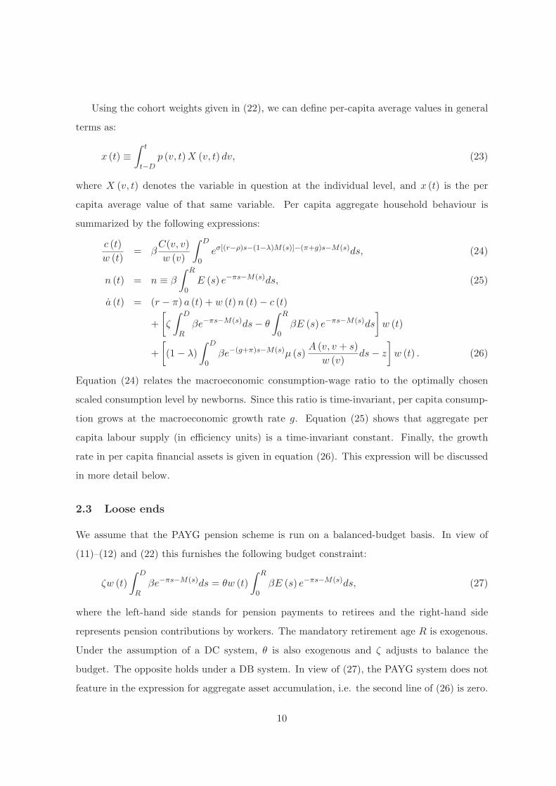
Using the cohort weights given in (22), we can define per-capita average values in general
terms as:
x (t) ≡
∫ t
t−Dp (v, t)X (v, t) dv, (23)
where X (v, t) denotes the variable in question at the individual level, and x (t) is the per
capita average value of that same variable. Per capita aggregate household behaviour is
summarized by the following expressions:
c (t)
w (t)= β
C(v, v)
w (v)
∫ D
0eσ[(r−ρ)s−(1−λ)M(s)]−(π+g)s−M(s)ds, (24)
n (t) = n ≡ β
∫ R
0E (s) e−πs−M(s)ds, (25)
a (t) = (r − π) a (t) + w (t)n (t) − c (t)
+
[
ζ
∫ D
Rβe−πs−M(s)ds − θ
∫ R
0βE (s) e−πs−M(s)ds
]
w (t)
+
[
(1 − λ)
∫ D
0βe−(g+π)s−M(s)µ (s)
A (v, v + s)
w (v)ds − z
]
w (t) . (26)
Equation (24) relates the macroeconomic consumption-wage ratio to the optimally chosen
scaled consumption level by newborns. Since this ratio is time-invariant, per capita consump-
tion grows at the macroeconomic growth rate g. Equation (25) shows that aggregate per
capita labour supply (in efficiency units) is a time-invariant constant. Finally, the growth
rate in per capita financial assets is given in equation (26). This expression will be discussed
in more detail below.
2.3 Loose ends
We assume that the PAYG pension scheme is run on a balanced-budget basis. In view of
(11)–(12) and (22) this furnishes the following budget constraint:
ζw (t)
∫ D
Rβe−πs−M(s)ds = θw (t)
∫ R
0βE (s) e−πs−M(s)ds, (27)
where the left-hand side stands for pension payments to retirees and the right-hand side
represents pension contributions by workers. The mandatory retirement age R is exogenous.
Under the assumption of a DC system, θ is also exogenous and ζ adjusts to balance the
budget. The opposite holds under a DB system. In view of (27), the PAYG system does not
feature in the expression for aggregate asset accumulation, i.e. the second line of (26) is zero.
10

Excess profits of annuity firms can be written as follows:
EP (v, t) ≡ (1 − λ)
∫ t
t−Dp (v, t)µ (t − v)A (v, t) dv. (28)
The integral on the right-hand side represents per capita annuitized assets of all individuals
that die in period t. This is the total revenue of annuity firms, of which only a fraction λ is
paid out to surviving annuitants. The remaining fraction, 1−λ, is excess profit which is taxed
away by the government and disbursed to all households in the form of lump-sum transfers,
i.e. EP (v, t) = TR (v, t). Using (13) and (28) we find the implied expression for z:
z = (1 − λ)
∫ D
0βe−(g+π)u−M(u)µ (u)
A (v, v + u)
w (v)du. (29)
Just as for the PAYG system, the redistribution of excess profits of annuity firms also debudget
from the asset accumulation equation, i.e. the third line in (26) is also zero.
In the absence of government bonds, the capital market equilibrium condition is given by
A (t) = K (t) or, in per capita average terms, by:
a (t) = k (t) , (30)
where k (t) ≡ K (t) /P (t) is the per capita stock of capital. From (5)–(6) we easily find:
y (t) = Ω0k (t) , (31)
w (t)n (t) = (1 − ε) y (t) , (32)
where y (t) ≡ Y (t) /P (t) is per capita output. From (26)–(27), (29) and (30) we can derive
the expression for the macroeconomic growth rate:
g ≡k (t)
k (t)= r − π +
[
n (t) −c (t)
w (t)
]
w (t)
k (t). (33)
For convenience, the key equations comprising the general equilibrium model have been
gathered in Table 1. Equations (T1.1)–(T1.2), (T1.3a)–(T1.3b), (T1.4)–(T1.6), (T1.8)–(T1.9)
restate, respectively, (16)–(17), (19)–(20), (27), (29), (33), (25), and (24). Equation (T1.7) is
obtained by combining (31) and (32) and noting (25).
The model features a two-way interaction between the microeconomic decisions and the
macroeconomic outcomes. Indeed, conditional on the macroeconomic variables, equations
(T1.1)–(T1.3) determine scaled newborn consumption and human wealth, C (v, v) /w (v) and
H (v, v) /w (v) as well as the age profile of scaled assets A (v, v + u) /w (v). Conditional on
11

these microeconomic variables, equations (T1.4)–(T1.9) determine equilibrium pension pay-
ments and transfers, ζ and z, the macroeconomic growth rate, g, the overall wage-capital
ratio, w (t) /k (t), aggregate labour supply, n, and the c (t) /w (t) ratio.
2.4 Adding empirical content
An important virtue of the analytical approach adopted here is that it allows one to pinpoint
the various places where life-cycle elements affect individual choices and aggregate outcomes.
The model contains three main mechanisms giving rise to life-cycle effects. First, the mortality
process is age-dependent, i.e. the instantaneous and cumulative hazard rates (µ (u) and
M (u)) both depend on age. Second, labour productivity (E (u)) depends on the worker’s
age. Third, the pension system and mandatory retirement age differentiates workers from
retirees. In the remainder of this section we add empirical content to the model by plausibly
calibrating the various life-cycle mechanisms.
To capture the demographic process we use the model suggested by Boucekkine et al.
(2002), which incorporates a finite maximum age. The surviving fraction up to age u (from
the perspective of birth) is given by:
e−M(u) ≡η0 − eη1u
η0 − 1, (34)
with η0 > 1 and η1 > 0. For this demographic process, D = (1/η1) ln η0 is the maximum
attainable age, whilst the instantaneous mortality rate at age u is given by:
µ (u) ≡η1e
η1u
η0 − eη1u. (35)
The mortality rate is increasing in age and becomes infinite at u = D.
In Heijdra and Mierau (2010) we use data from age 18 onward for the Dutch cohort that
was born in 1960. We denote the actual surviving fraction up until model age ui by Si, and
estimate the parameters of the parametric distribution function by means of non-linear least
squares. The model to be estimated is thus:
Si = 1 − Φ(ui) + εi = d (ui ≤ D) ·η0 − eη1ui
η0 − 1+ εi, (36)
where d (ui ≤ D) = 1 for ui ≤ D, and d (ui ≤ D) = 0 for ui > D, and εi is the stochastic error
term. We find the following estimates (with t-statistics in brackets): η0 = 122.643 (11.14),
12
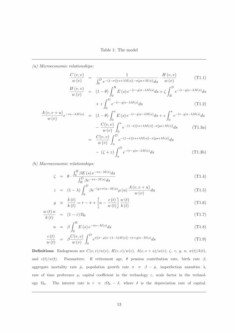
Table 1: The model
(a) Microeconomic relationships:
C (v, v)
w (v)=
1∫ D0 e−(1−σ)[rs+λM(s)]−σ[ρs+M(s)]ds
·H (v, v)
w (v)(T1.1)
H (v, v)
w (v)= (1 − θ)
∫ R
0E (s) e−(r−g)s−λM(s)ds + ζ
∫ D
Re−(r−g)s−λM(s)ds
+ z
∫ D
0e−(r−g)s−λM(s)ds (T1.2)
A (v, v + u)
w (v)e−ru−λM(u) = (1 − θ)
∫ u
0E (s) e−(r−g)s−λM(s)ds + z
∫ u
0e−(r−g)s−λM(s)ds
−C(v, v)
w (v)
∫ u
0e−(1−σ)[rs+λM(s)]−σ[ρs+M(s)]ds (T1.3a)
=C(v, v)
w (v)
∫ D
ue−(1−σ)[rs+λM(s)]−σ[ρs+M(s)]ds
− (ζ + z)
∫ D
ue−(r−g)s−λM(s)ds (T1.3b)
(b) Macroeconomic relationships:
ζ = θ ·
∫ R0 βE (s) e−πs−M(s)ds
∫ DR βe−πs−M(s)ds
(T1.4)
z = (1 − λ)
∫ D
0βe−(g+π)u−M(u)µ (u)
A (v, v + u)
w (v)du (T1.5)
g ≡k (t)
k (t)= r − π +
[
n −c (t)
w (t)
]
w (t)
k (t)(T1.6)
w (t)n
k (t)= (1 − ε) Ω0 (T1.7)
n = β
∫ R
0E (s) e−πs−M(s)ds (T1.8)
c (t)
w (t)= β
C(v, v)
w (v)
∫ D
0eσ[(r−ρ)s−(1−λ)M(s)]−(π+g)s−M(s)ds (T1.9)
Definitions: Endogenous are C(v, v)/w(v), H(v, v)/w(v), A(v, v + u)/w(v), ζ, z, g, n, w(t)/k(t),
and c(t)/w(t). Parameters: R retirement age, θ pension contribution rate, birth rate β,
aggregate mortality rate µ, population growth rate π ≡ β − µ, imperfection annuities λ,
rate of time preference ρ, capital coefficient in the technology ε, scale factor in the technol-
ogy Ω0. The interest rate is r ≡ εΩ0 − δ, where δ is the depreciation rate of capital.
13

η1 = 0.0680 (48.51). The standard error of the regression is σ = 0.02241, and the implied
estimate for D is 70.75 model years (i.e., the maximum age in biological years is 88.75).
Figure 1(a) depicts the actual and fitted survival rates with, respectively, solid and dashed
lines. Up to age 69, the model fits the data rather well. For higher ages the fit deteriorates
as the estimated model fails to capture the fact that some people are expected to live very
long lives in reality. Figure 1(b) depicts the implies instantaneous mortality rate. Mortality
is very low and virtually constant up to model age u = 50 (corresponding with biological age
68) but rises at an increasing rate thereafter. Finally, Figure 1(c) shows the implied relative
cohort sizes.
Several studies have argued that labour productivity is hump-shaped – see for example
Hansen (1993) and Rios-Rull (1996).4 An analytically convenient age profile for productivity
involves exponential terms:
E (u) = α0e−ζ0u − α1e
−ζ1u, (37)
where E (u) is labour productivity of a u-year old worker, and we assume that α0 > α1 > 0,
ζ1 > ζ0 > 0, and α1ζ1 > α0ζ0. We easily find that E (u) ≥ 0, E (0) = α0 − α1 > 0,
limu→∞ E (u) = 0, E′ (u) > 0 (for 0 ≤ u < u) and E′ (u) < 0 (for u ≥ u) where the peak
occurs at age u:
u =1
ζ1 − ζ0
ln
(
α1ζ1
α0ζ0
)
. (38)
Labour productivity is non-negative throughout life, starts out positive, is rising during the
first life phase, and declines thereafter. Using cross-section efficiency data for male workers
aged between 18 and 70 from Hansen (1993, p. 74) we find the solid pattern in Figure 1(d).
We interpolate these data by fitting equation (37) using non-linear least squares. We find
the following estimates (t-statistics in brackets): α0 = 4.494 (fixed), α1 = 4.010 (71.04),
ζ0 = 0.0231 (24.20), and ζ1 = 0.050 (17.81). The fitted productivity profile is illustrated with
dashed lines in Figure 1(d).
Finally, for the third life-cycle feature – the PAYG pension system – we assume that the
mandatory retirement age is set at R = 47 (corresponding with 65 in biological years) and
that the pension contribution rate is seven percent of wage income, i.e. θ = 0.07 which roughly
4The relationship between age and worker productivity is studied in a number of recent papers by Lallemand
and Rycx (2009) and van Ours (2009).
14

Figure 1: Life-cycle features
(a) mortality process (b) instantaneous mortality rate
e−M(u) µ(u)
20 30 40 50 60 70 80 90 1000
0.1
0.2
0.3
0.4
0.5
0.6
0.7
0.8
0.9
1
biological age (u+18)
DataEstimates
20 30 40 50 60 70 80 90 1000
0.05
0.1
0.15
0.2
0.25
0.3
0.35
0.4
biological age (u+18)
20102040
(c) relative cohort size (d) efficiency profile
βe−πu−M(u) E(u)
20 30 40 50 60 70 80 90 1000
0.005
0.01
0.015
0.02
0.025
biological age (u+18)
20102040
20 25 30 35 40 45 50 55 60 65 70 750
0.2
0.4
0.6
0.8
1
1.2
1.4
1.6
biological (u+18)
DataEstimates
Notes: u is the agent’s age, β is the crude birth rate, π is the population growth rate, M(u) is the
cumulative mortality factor, µ(u) is the instantaneous mortality rate, and E(u) is labour productivity
at age u. The maximum attainable age estimated with Dutch data is D = 70.75.
15

corresponds with the Dutch pension system. The implied pension benefit is determined in
general equilibrium.
The remainder of the core model is parameterized as follows. We postulate the existence
of perfect annuities (PA, with λ = 1). We assume that the rate of population growth is half
of one percent per annum (π = 0.005). For the estimated demographic process, equation
(21) yields a steady-state birth rate equal to β = 0.0204. Since µ ≡ β − π, this implies that
the average mortality rate is µ = 0.0154. The old-age dependency ratio equals 22.92%. We
model an economy with a steady-state capital-output ratio of 2.5, which is obtained by setting
Ω0 = 0.4. The interest rate is five percent per annum (r = 0.05), the capital depreciation
rate is seven percent per annum (δ = 0.07), and the efficiency parameter of capital is set at
ε = 0.3. The steady-state growth rate is set equal to two percent per annum (g = 0.02). For
the intertemporal substitution elasticity we use σ = 0.7, a value consistent with the estimates
reported by Attanasio and Weber (1995). The rate of pure time preference is used as a
calibration parameter, yielding a value of ρ = 0.0112.
Table 2(a) reports the main features of the initial steady-state growth path. With perfect
annuities, there are no excess profits of annuity firms and thus no transfers, i.e. z = 0 in
Table 2(a). Note also that at retirement age R a vintage-v agent receives ζw (v + R) in the
form of a pension whereas the last-received wage for this agent equals E (R) w (v + R). The
replacement rate is thus equal to ζ/E (R) = 0.3189.
We visualize the life-cycle profiles for a number a key variables in Figure 2. The solid lines
are associated with the core model featuring perfect annuities. For ease of interpretation, the
horizontal axes report biological age, u + 18. Figure 2(a) shows that with perfect longevity
insurance consumption rises monotonically over the life cycle. This counterfactual result
follows readily from (18) which for λ = 1 simplifies to C (v, τ) /C (v, τ) = σ (r − ρ). Figure
2(b) depicts the age profile of scaled financial assets. At first the agent is a net borrower,
i.e. a buyer of life-insured loans. Thereafter annuity purchases are positive and the profile
of assets is bell-shaped. In the absence of a bequest motive, the agent plans to run out of
financial assets at the maximum age D. Figure 2(c) shows the profile of scaled wages over
the life cycle. Despite the fact that individual labour productivity itself is bell-shaped (see
Figure 1(d)), wages increase monotonically as a result of ongoing economic growth. Finally,
in Figure 2(d) we illustrate the profile for scaled pension receipts. During the working career
16

Table 2: Quantitative effects
(a) (b) (c) (d) (e) (f) (g) (h)
Case: PA IA PA IA PA IA PA IA
Core cases DC DB RAC (v, v)
w (v)0.8534 0.8609 1.0784 1.0785 0.9078 0.9053 0.9329 0.9369
H (v, v)
w (v)26.5646 27.0207 36.0229 36.2942 30.3246 30.4653 31.1617 31.5282
g (%) 2.00 1.91 3.36 3.27 2.79 2.68 2.39 2.30
n 0.9675 0.9675 0.8212 0.8212 0.8212 0.8212 0.9589 0.9589
w (t)
k (t)0.2894 0.2894 0.3410 0.3410 0.3410 0.3410 0.2920 0.2920
c (t)
w (t)1.0538 1.0570 0.8692 0.8720 0.8861 0.8893 1.0482 1.0514
ζ 0.3632 0.3632 0.1824 0.1824 0.3632 0.3632 0.3632 0.3632
z 0.0200 0.0142 0.0131 0.0185
θ 0.1394 0.1394
R + 18 75.3 75.3
Notes. PA stands for perfect annuities (λ = 1) and IA denotes imperfect annuities (λ = 0.7).
Column (a) is the core model. Column (b) shows the effects of the annuity market imperfection in the
core model. Columns (c)–(d) show the effects of a demographic shock under a DC pension system.
Columns (e)–(f) show the effects under a DB system. In this scenario the tax rate θ adjusts to keep
ζ at its pre-shock level. Columns (g)–(h) show the effects under a retirement age (RA) scenario in
which θ and ζ are kept at their pre-shock levels and R is adjusted.
17
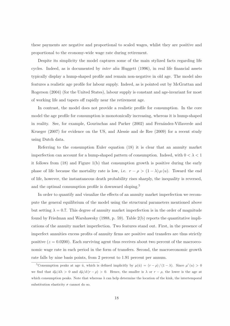
these payments are negative and proportional to scaled wages, whilst they are positive and
proportional to the economy-wide wage rate during retirement.
Despite its simplicity the model captures some of the main stylized facts regarding life
cycles. Indeed, as is documented by inter alia Huggett (1996), in real life financial assets
typically display a hump-shaped profile and remain non-negative in old age. The model also
features a realistic age profile for labour supply. Indeed, as is pointed out by McGrattan and
Rogerson (2004) (for the United States), labour supply is constant and age-invariant for most
of working life and tapers off rapidly near the retirement age.
In contrast, the model does not provide a realistic profile for consumption. In the core
model the age profile for consumption is monotonically increasing, whereas it is hump-shaped
in reality. See, for example, Gourinchas and Parker (2002) and Fernandez-Villaverde and
Krueger (2007) for evidence on the US, and Alessie and de Ree (2009) for a recent study
using Dutch data.
Referring to the consumption Euler equation (18) it is clear that an annuity market
imperfection can account for a hump-shaped pattern of consumption. Indeed, with 0 < λ < 1
it follows from (18) and Figure 1(b) that consumption growth is positive during the early
phase of life because the mortality rate is low, i.e. r − ρ > (1 − λ)µ (u). Toward the end
of life, however, the instantaneous death probability rises sharply, the inequality is reversed,
and the optimal consumption profile is downward sloping.5
In order to quantify and visualize the effects of an annuity market imperfection we recom-
pute the general equilibrium of the model using the structural parameters mentioned above
but setting λ = 0.7. This degree of annuity market imperfection is in the order of magnitude
found by Friedman and Warshawsky (1988, p. 59). Table 2(b) reports the quantitative impli-
cations of the annuity market imperfection. Two features stand out. First, in the presence of
imperfect annuities excess profits of annuity firms are positive and transfers are thus strictly
positive (z = 0.0200). Each surviving agent thus receives about two percent of the macroeco-
nomic wage rate in each period in the form of transfers. Second, the macroeconomic growth
rate falls by nine basis points, from 2 percent to 1.91 percent per annum.
5Consumption peaks at age u, which is defined implicitly by µ(u) = (r − ρ) / (1 − λ). Since µ′ (u) > 0
we find that dµ/dλ > 0 and dµ/d (r − ρ) > 0. Hence, the smaller is λ or r − ρ, the lower is the age at
which consumption peaks. Note that whereas λ can help determine the location of the kink, the intertemporal
substitution elasticity σ cannot do so.
18

The ultimate effect on newborn consumption of the change in λ depends on the interplay
between the human wealth effect and the propensity effect. Recall from (T1.1)–(T1.2) that
C (v, v) = ∆ · H (v, v) where the propensity to consume is defined as:
∆ ≡1
∫ D0 e−(1−σ)[rs+λM(s)]−σ[ρs+M(s)]ds
. (39)
It is easy to show that with 0 < σ < 1, the propensity to consume out of human wealth falls
as a result of the reduction in λ:
d∆
dλ= (1 − σ) ∆2 ·
∫ D
0M (s) e−(1−σ)[rs+λM(s)]−σ[ρs+M(s)]ds > 0. (40)
The partial derivative of scaled human wealth with respect to λ is given by:
∂
∂λ
H (v, v)
w (v)= − (1 − θ)
∫ R
0M (s) E (s) e−(r−g)s−λM(s)ds − ζ
∫ D
RM (s) e−(r−g)s−λM(s)ds
−z
∫ D
0M (s) e−(r−g)s−λM(s)ds < 0. (41)
A decrease in λ results in a reduction in the annuity rate of interest at all age levels and
thus an increase in human wealth due to less severe discounting of non-asset income streams.
Human wealth is also affected by two of the macroeconomic variables, namely transfers z
and the growth rate g (note that n, ζ, and w (t) /k (t) are not affected by λ). Scaled human
wealth is boosted as a result of the transfers:
∂
∂z
H (v, v)
w (v)=
∫ D
0e−(r−g)s−λM(s)ds > 0, (42)
but it is reduced by the decrease in the growth rate:
∂
∂g
H (v, v)
w (v)= (1 − θ)
∫ R
0sE (s) e−(r−g)s−λM(s)ds + ζ
∫ D
Rse−(r−g)s−λM(s)ds
+z
∫ D
0se−(r−g)s−λM(s)ds > 0. (43)
The results in Table 2(b) confirm that for our parameterization scaled consumption and
human wealth both increase, i.e. the effects in (41) and (42) dominate the combined propen-
sity effect (40) and growth effect (43).
In Figure 2 the dashed lines depict the life-cycle profiles associated with the model featur-
ing imperfect annuities. Scaled consumption is hump-shaped but peaks at a rather high age.6
6Butler (2001) and Hansen and Imrohoroglu (2008) also find that the hump occurs too late in life. Alessie
and de Ree (2009, p. 113) decompose Dutch consumption into durables and non-durables. They find that
non-durable consumption peaks at age 45 whereas durable consumption reaches its maximum at about age 41.
19

Figure 2: Life-cycle profiles and the role of annuity imperfections
(a) scaled consumption (b) scaled financial assets
C(v, v + u)
w(v)
A(v, v + u)
w(v)
20 30 40 50 60 70 800
1
2
3
4
5
6
biological age (u+18)
Perfect AnnuitiesImperfect Annuities
20 30 40 50 60 70 80−5
0
5
10
15
20
25
30
biological age (u+18)
Perfect AnnuitiesImperfect Annuities
(c) scaled wage rate (d) scaled pension receipts
w(v, v + u)
w(v)
PR(v, v + u)
w(v)
20 30 40 50 60 70 800
0.5
1
1.5
2
2.5
3
3.5
biological age (u+18)
Perfect AnnuitiesImperfect Annuities
20 30 40 50 60 70 80−0.4
−0.2
0
0.2
0.4
0.6
0.8
1
1.2
1.4
1.6
biological age (u+18)
Perfect AnnuitiesImperfect Annuities
20

The profiles for scaled financial assets, wages, and pension payments are all very similar to
the ones for the core model.7
3 Ageing: the big picture
In this section we put our model to work on the big policy issue of demographic change.
Population ageing remains one of the key issues in economic policy in the Netherlands. During
the 2010 Dutch parliamentary election campaign numerous parties went so far as to call future
policy on pensions and the retirement age a breaking point for the post-electoral coalition
scramble. In this section we look at the big picture and study the effect of ageing and
demographic change on the steady-state rate of economic growth of a country.8
We start our analysis with some stylized facts for the Netherlands.9 In the period 2005-10
the crude birth rate is about β = 1.13% per annum whereas for 2035-40 it is projected to
change to β = 1.05% per annum. The population growth rates are, respectively, π = 0.41%
per annum for 2005-10 and π = −0.01% per annum 2035-40. Finally, the old-age dependency
ratio is, respectively 23% in 2010 and 46% in 2040. We wish to simulate our model using
a demographic shock which captures the salient features of these stylized facts. Since we
restrict attention to steady-state comparisons in this paper, we make the strong assumption
that the country finds itself in a demographic steady state both at present and in 2040.
3.1 A demographic shock
The demographic shock that we study is as follows. First, we assume that the population
growth rate changes from π0 = 0.5% to π1 = 0% per annum. Second, we use our esti-
mated demographic process (34) but change the η1 parameter in such a way that an old-age
7We study the consequences of annuitization for economic growth and individual welfare in Heijdra and
Mierau (2009, 2010) and Heijdra, Mierau and Reijnders (2010). The latter paper demonstrates the existence
of a “tragedy of annuitization”. Although full annuitization of assets is privately optimal it may not be socially
beneficial due to adverse general equilibrium repercussions.8For an accessible survey of the literature on the topic of population ageing and economic growth, see
Bloom et al. (2008). Recent contributions using the endogenous growth framework include Fougere and
Merette (1999), Futagami and Nakajima (2001), Heijdra and Romp (2006), and Prettner (2009).9These figures are taken from United Nations, World Population Prospects: The 2008 Revision Population
Data Base, http://esa.un.org/unpp. We use data for the medium variant.
21

dependency ratio of 46% is obtained. Writing e−Mi(u) ≡ (η0 − eη1,iu) / (η0 − 1) the old-age
dependency ratio can be written as:
dr(
πi, η1,i
)
≡
∫ Di
47 e−πis−Mi(s)ds∫ 470 e−πis−Misds
, (44)
where Di ≡(
1/η1,i
)
ln η0. Using this expression we find that η1 changes from η1,0 = η1 =
0.0680 to η1,1 = 0.0581. The associated values for the crude birth rate are by imposing the
suitably modified demographic steady-state condition (21). We find that β changes in the
model from β0 = 0.0204 to β1 = 0.0151. Figure 1(b) shows that the new instantaneous
mortality profile shifts to the right. Figure 1(c) illustrates the change in the population
composition. In the new steady state, the population distribution features less mass at lower
ages and more at higher ages, i.e. the population pyramid becomes narrower and higher.
The effect on the economic growth rate of the demographic shock depends critically on
the type of pension system. We consider three scenarios. In the first scenario the pension
system is DC, the contribution rate and retirement age are kept constant (θ0 = 0.07 and
R0 = 47), pension payments to the elderly are reduced to balance the budget of the PAYG
system. Columns (c)–(d) in Table 2 report the results for the two cases with perfect (PA)
and imperfect annuities (PA). Since the effects are qualitatively the same for PA and IA,
we restrict attention to the latter case. Comparing columns (b) and (d) several features
stand out. First, the ageing shock has a large effect on the supply of (efficiency units of)
labour, i.e. n falls by more than fifteen percent. This is an obvious consequence of the fact
that the population proportion of working-age persons declines (see Figure 1(d)). Second,
the pension payments to retirees are almost halved. Third, notwithstanding the decrease in
pensions, scaled consumption and human wealth at birth both increase dramatically. More
people expect to survive into retirement and, once retired, the period of retirement is also
increased. Fourth, the macroeconomic growth rate increases dramatically, from 1.91% to
3.27% per annum. The intuition behind this strong growth effect can be explained with the
aid of Figure 3. The solid lines represents the core case of Table 2(b) and the dashed lines
illustrate the results from Table 2(d). Following the demographic shock scaled consumption is
uniformly higher and peaks at a later age. Scaled financial assets are somewhat lower during
youth but much higher thereafter. As Figure 3(b) shows there is a huge savings response
which explains the large increase in the macroeconomic growth rate. In conclusion, of the
22

main growth channels identified by Bloom et al. (2008, p. 2), labour supply falls (and thus
retards growth) but the capital accumulation effect is so strong as to lead to a strong positive
effect of longevity on economic growth.
In the second scenario the pension system is DB, the pension payments and retirement
age are kept constant (ζ0 = 0.3632 and R0 = 47), and pension contributions by the young are
increased to balance the budget of the PAYG system. Columns (e)–(f) in Table 2 give the
results for this case. Comparing columns (b), (d) and (f) the following features stand out.
First, the contribution rate increased is quite substantial, it almost doubles from θ0 = 0.07
to θ1 = 0.1394. Second, though scaled consumption, scaled human wealth, and the economic
growth rate are higher than in the base case, they are lower than under the DC scenario.
As Figure 3 shows, the capital accumulation effect of the longevity shock is substantially
dampened under a DB system. Intuitively, by taking from the young and giving to the old
the PAYG system redistributes from net savers to net dissavers.
Finally, in the third scenario both θ and ζ are kept at their pre-shock levels and the
retirement age is increased to balance the budget of the PAYG system. Columns (g)–(h)
in Table 2 give the results for this case. Comparing columns (b), (d), (f), and (h) the
following features stand out. First, under the retirement age (RA) scenario the longevity
shock necessitates an increase in the biological retirement age 65 to 75.3 years. i.e. the value
of R restoring budget balance changes from R0 = 47 to R1 = 57.3. Second, compared to the
DB and DC cases, labour supply increases strongly in the RA scenario. Third, the economic
growth rate, though still higher than in the base case, is slightly lower that under DB and
much lower than under DC. The intuition behind this result is clear from Figure 3(b) which
shows that the savings response following the longevity shock is lower than either DB or DC.
3.2 Robustness
The clear message emerging from the discussion so far is that the type of pension system in
place has a quantitatively large influence on the link between longevity and macroeconomic
growth. Indeed, the same longevity shock can either lead to a huge increase in growth (under
DC) or only a modest increase (under RA). But how robust are these conclusions? As is
pointed out by Bloom et al. (2008, p. 3), “population data are not sacrosanct” and UN
predictions are revised substantially over time. In short, our stylized demographic facts may
23

be more like “factoids”.10
We study the robustness issue in Table 3. We restrict attention to the case with imperfect
annuities, and column (a) in the table represents the base case. It coincides with the pre-shock
steady state reported in Table 2(b). Columns (b)–(c) in Table 3 report the results under the
DC scenario for alternative demographic shocks. In contrast, columns (d)-(e) show how a
much more broadly defined PAYG system reacts to the original demographic shock under
DC, DB, and RA.
In column (b) we assume that the old-age dependency ratio is 30% rather than 46% in 2040.
As in the original shock we continue to assume that π1 = 0% per annum. By using (44) we
obtain new values for the demographic parameters, i.e. η1,1 = 0.0662 and β1 = µ1 = 0.0172.
The alternative demographic shock causes a small increase in the economic growth rate.
Whereas the original demographic shock caused growth to increase from 1.91% to 3.27%
per annum (See Table 2, columns (b) and (d)), the alternative one only raises the growth
rate to 2.33% per annum. The alternative ageing shock is relatively small, and pensions are
reduced much less drastically than under the original demographic shock. The private savings
response is quite small as a result.
In column (c) we keep the dependency ratio at 46% but assume that the population growth
rate is 0.5% rather than 0% per annum in 2040. Under this assumption the demographic pa-
rameters are equal to η1,1 = 0.0540, β1 = 0.0168, and µ1 = 0.0118. This type of demographic
shock produces a huge increase in the macroeconomic growth rate. The intuition is the same
as before – see the discussion relating to Table 2(d) above. The large growth effect is all
the more surprising in view of the growth equation (T1.6) which directly features −π on the
right-hand side. So even though the demographic shock itself retards growth by 0.5% per
annum, the huge private savings response more than compensates for this effect.
In conclusion, the two alternative demographic shocks give rise to qualitatively the same
predictions as we obtained for the original shock. Under a DC system economic growth is
boosted because the labour supply effect is strongly dominated by the capital accumulation
effect.
As a final robustness check we investigate whether the size of the PAYG system influ-
10De Waegenaere et al. (2010) provide a survey of the recent literature on longevity risk (i.e. the risk that
mortality predictions turn out to be wrong). In accordance with Bloom et al. (2008) they show that estimates
on future mortality rates differ substantially and depend on a plethora of uncertain factors.
24

ences the relationship between longevity and economic growth. We return to the original
demographic shock featuring π1 = 0.05% per annum and an old-age dependency ratio of 46%
(η1,1 = 0.0581 and β1 = 0.0151). As was pointed out by Broer (2001, p. 89), “in an ageing
society, both the health insurance system and the pension system impose an increasing bur-
den on households. . . . Thus as the share of elderly in the population grows, the contribution
base [of the public health insurance system, HM] shrinks at the same time when demand for
health care increases.” In short, it can be argued that the public health insurance system
itself contains elements of a PAYG type, i.e. it taxes the young (and healthy) and provides
resources to the old (and infirm).
Whereas it is beyond the scope of the present paper to fully model the health insurance
system, we take from Broer’s analysis the idea that the PAYG system may be broader than
just the public pension system itself. We study the quantitative consequences of PAYG
system size in columns (d)–(g) in Table 3. Column (d) shows what happens to the initial
steady-state economy if the contribution rate is increased from θ0 = 0.07 to θ1 = 0.15. The
comparison between columns (a) and (d) reveals that there is a huge drop in the growth
rate, from g = 1.91% to g = 1.19% per annum. Intuitively the larger PAYG system takes
more from the young and gives more to the old. This chokes off private savings and retards
economic growth.
Columns (e)–(g) in Table 3 shows the effects of the original demographic shock under
DC, DB, and RA. The growth increases under all scenarios with the largest effect occurring
under the DC system. Interestingly, whereas the growth effect was smallest for the RA case
in the original model with the narrowly defined PAYG system, for a large PAYG system it is
smallest for the DB scenario.
3.3 Limitations
A few words of caution are in place when interpreting our conclusions. There are several
limitations. First, our analysis consists of steady-state comparisons and space considerations
prevent us from studying the transitional dynamics of a longevity shock. Although we find
that in the steady state a longevity shock has beneficial effects on growth, it need not be the
case that transition is monotonic. Second, we have merely analyzed growth but not individ-
ual welfare. However, as we assume exogenous labour supply higher growth automatically
25

Table 3: Alternative scenarios
Initial PAYG system Large PAYG system
(a) (b) (c) (d) (e) (f) (g)
DC DC DC DB RA
C (v, v)
w (v)0.8609 0.9268 1.0971 0.7047 0.8818 0.6109 0.7678
H (v, v)
w (v)27.0207 29.4510 38.0243 22.1187 29.6744 20.5594 25.8384
g (%) 1.91 2.33 3.43 1.19 2.59 1.51 1.71
n 0.9675 0.9217 0.8155 0.9675 0.8212 0.8212 0.9589
w (t)
k (t)0.2894 0.3038 0.3434 0.2894 0.3410 0.3410 0.2920
c (t)
w (t)1.0570 1.0094 0.8465 1.0817 0.8918 0.9236 1.0715
ζ 0.3632 0.2796 0.1812 0.7783 0.3910 0.7783 0.7783
z 0.0200 0.0200 0.0111 0.0174 0.0130 0.0120 0.0148
θ 0.2986
R + 18 75.3
Notes. Column (a) is the core model with imperfect annuities (column (b) in Table 2). Column
(b) dependency ratio in 2040 equal to 30% instead of 46%. Column (c) population growth rate in
2040 equal to 0.5% instead of 0% per annum. Column (d) bigger PAYG system (θ = 0.15). Columns
(e)–(f) show the effects of the original demographic shock for the large PAYG system under DC and
DB. Column (g) leaves θ and ζ unchanged and features a higher retirement age.
26

Figure 3: Life-cycle profiles before and after the demographic shock
(a) scaled consumption (b) scaled financial assets
C(v, v + u)
w(v)
A(v, v + u)
w(v)
20 30 40 50 60 70 80 90 1000
1
2
3
4
5
6
7
biological age (u+18)
20102040 (DC)2040 (DB)2040 (RA)
20 30 40 50 60 70 80 90 100−10
0
10
20
30
40
50
biological age (u+18)
20102040 (DC)2040 (DB)2040 (RA)
translates into higher welfare because discounted income of individuals increases. Third, we
have assumed that labour supply and the retirement age are exogenous. We have chosen this
approach here in order to keep the model as simple as possible. Indeed, endogenization of
both the hours decision over the life cycle and/or the retirement date is fairly straightforward
– see e.g. Heijdra and Romp (2009) and Heijdra and Mierau (2009, 2010). Fourth, we have
ignored aggregate risk and the risk-sharing properties of pension systems. The interested
reader is referred to Bovenberg and Uhlig (2008) who apply a two-period stochastic overlap-
ping generations model featuring endogenous growth to study the consequences of particular
pension systems on risk-sharing between generations. Finally, we have studied a closed econ-
omy. This is not a convincing representation of the Dutch economy which is extremely open
and small in world markets. However, aging is a global phenomenon. Hence, to model a
small open economy with fixed factor prices is equally unconvincing. Here we have chosen
the closed economy framework to zoom in on the global consequences of ageing on capital
accumulation and economic growth – the big picture.
27

4 Conclusions
We develop a macroeconomic model that is firmly grounded in the microeconomic environ-
ment of the individual. In contrast to the highly stylized models in the tradition of Blanchard
(1985) we are able to replicate individual profiles for both consumption and savings. In
addition, and in contrast to the very detailed computable general equilibrium models, we
are still able to clearly analyze the mechanisms that are at play in the interaction between
microeconomic behaviour and macroeconomic outcomes.
For the purpose at hand we have kept the model as simple as possible. The model, however,
is very flexible in its very nature. In earlier work we have used a more elaborate version of
the model to study issues relating to capital market imperfections (Heijdra and Mierau, 2009)
and taxation issues (Heijdra and Mierau, 2010). In future work we seek to further study the
nebulous relationship between aging and economic growth in a model where also the labour
market participation decision (concerning entry and retirement) is made endogenous.
With the current version of the model we study the relationship between aging and eco-
nomic growth and the mediating role that government policy has on this relationship. We
find that, in principle, aging increases the economic growth rate. However, if a defined benefit
system is in place the growth effect weakens somewhat because of the increase in the contribu-
tion rate necessary to finance the additional pensioners. In order to circumvent this adverse
effect on the growth rate the government might consider to switch to a defined contribution
system or to increase the retirement age. Surprisingly, we find that the latter policy option
has adverse effects on the economy. This is due to a weaker savings reaction to the shortened
retirement horizon.
28

References
Abel, A. B. (1986). Capital accumulation and uncertain lifetimes with adverse selection.
Econometrica, 54:1079–1098.
Alessie, R. and de Ree, J. (2009). Explaining the hump in life cycle consumption profiles. De
Economist, 157:107–120.
Attanasio, O. P. and Weber, G. (1995). Is consumption growth consistent with intertemporal
optimization? Evidence from the consumer expenditure survey. Journal of Political
Economy, 103:1121–1157.
Auerbach, A. J. and Kotlikoff, L. J. (1987). Dynamic Fiscal Policy. Cambridge University
Press, Cambridge.
Blanchard, O.-J. (1985). Debts, deficits, and finite horizons. Journal of Political Economy,
93:223–247.
Bloom, D. E., Canning, D., and Fink, G. (2008). Population aging and economic growth.
Working Paper 320, Commission on Growth and Development, Washington, DC.
Boucekkine, R., de la Croix, D., and Licandro, O. (2002). Vintage human capital, demographic
trends, and endogenous growth. Journal of Economic Theory, 104:340–375.
Bovenberg, A. L. and Uhlig, H. (2008). Pension systems and the allocation of macroeconomic
risk. NBER International Seminar on Macroeconomics 2006, pages 241–323.
Broer, D. P. (2001). Growth and welfare distribution in an ageing society: An applied general
equilibrium analysis for the Netherlands. De Economist, 149:81–114.
Butler, M. (2001). Neoclassical life-cycle consumption: A textbook example. Economic
Theory, 17:209–221.
d’Albis, H. (2007). Demographic structure and capital accumulation. Journal of Economic
Theory, 132:411–434.
De Waegenaere, A., Melenberg, B., and Stevens, R. (2010). Longevity risk. De Economist,
158:151–192.
29

Fehr, H. (2009). Computable stochastic equilibrium models and their use in pension- and
ageing research. De Economist, 157:359–416.
Fernandez-Villaverde, J. and Krueger, D. (2007). Consumption over the life cycle: Facts from
consumer expenditure survey data. Review of Economics and Statistics, 89:552–565.
Finkelstein, A. and Poterba, J. (2002). Selection effects in the United Kingdom individual
annuities market. Economic Journal, 112(476):28–50.
Fougere, M. and Merette, M. (1999). Population ageing and economic growth in seven OECD
countries. Economic Modelling, 16:411–427.
Friedman, B. M. and Warshawsky, M. J. (1988). Annuity prices and saving behavior in the
United States. In Bodie, Z., Shoven, J. B., and Wise, D. A., editors, Pensions in the U.S
Economy, pages 53–77. University of Chicago Press, Chicago.
Futagami, K. and Nakajima, T. (2001). Population aging and economic growth. Journal of
Macroeconomics, 23:31–44.
Gourinchas, P.-O. and Parker, J. A. (2002). Consumption over the life cycle. Econometrica,
70:47–89.
Hansen, G. D. (1993). The cyclical and secular behaviour of the labour input: Comparing
efficiency units and hours worked. Journal of Applied Econometrics, 8:71–80.
Hansen, G. D. and Imrohoroglu, S. (2008). Consumption over the life cycle: The role of
annuities. Review of Economic Dynamics, 11:566–583.
Heijdra, B. J. and Mierau, J. O. (2009). Annuity market imperfection, retirement and eco-
nomic growth. Working Paper 2717, CESifo, Munchen.
Heijdra, B. J. and Mierau, J. O. (2010). Growth effects of consumption and labour-income
taxation in an overlapping-generations life-cycle model. Macroeconomic Dynamics, 14.
Heijdra, B. J., Mierau, J. O., and Reijnders, L. S. M. (2010). The tragedy of annuitization.
Working Paper 3141, CESifo, Munchen.
Heijdra, B. J. and Reijnders, L. S. M. (2009). Economic growth and longevity risk with
adverse selection. Working Paper 2898, CESifo, Munchen.
30

Heijdra, B. J. and Romp, W. E. (2006). Ageing and growth in the small open economy.
Working Paper 1740, CESifo, Munchen.
Heijdra, B. J. and Romp, W. E. (2008). A life-cycle overlapping-generations model of the
small open economy. Oxford Economic Papers, 60:89–122.
Heijdra, B. J. and Romp, W. E. (2009). Retirement, pensions, and ageing. Journal of Public
Economics, 93:586–604.
Huggett, M. (1996). Wealth distribution in life-cycle economies. Journal of Monetary Eco-
nomics, 38:469–494.
Lallemand, T. and Rycx, F. (2009). Are older workers harmful for firm productivity? De
Economist, 157:273–292.
McGrattan, E. R. and Rogerson, R. (2004). Changes in hours worked, 1950-2000. Federal
Reserve Bank of Minneapolis Quarterly Review, 28:14–33.
Pissarides, C. A. (1980). The wealth-age relation with life insurance. Economica, 47:451–457.
Prettner, K. (2009). Population ageing and endogenous economic growth. Working Paper
8-2009, Vienna Institute of Demography, Vienna, Austria.
Rıos-Rull, J. V. (1996). Life-cycle economies and aggregate fluctuations. Review of Economic
Studies, 63:465–489.
Romer, P. M. (1989). Capital accumulation in the theory of long-run growth. In Barro, R. J.,
editor, Modern Business Cycle Theory, pages 51–127. Basil Blackwell, Oxford.
Sims, C. (1980). Macroeconomics and reality. Econometrica, 48(1):1–48.
van Ours, J. (2009). Will you still need me: When I’m 64? De Economist, 157:441–460.
Yaari, M. E. (1965). Uncertain lifetime, life insurance, and the theory of the consumer. Review
of Economic Studies, 32:137–150.
31