The importance of correcting for sampling bias in MaxEnt species ...

BIODIVERSITYRESEARCH

The importance of correcting forsampling bias in MaxEnt speciesdistribution modelsStephanie Kramer-Schadt1*, J€urgen Niedballa1, John D. Pilgrim2,

Boris Schr€oder3,4, Jana Lindenborn1, Vanessa Reinfelder1, Milena Stillfried1,

Ilja Heckmann1, Anne K. Scharf1, Dave M. Augeri5,6, Susan M. Cheyne7,8,

Andrew J. Hearn7, Joanna Ross7, David W. Macdonald7, John Mathai9†,

James Eaton10, Andrew J. Marshall11, Gono Semiadi12, Rustam Rustam13,

Henry Bernard14, Raymond Alfred15, Hiromitsu Samejima16,

J. W. Duckworth17, Christine Breitenmoser-Wuersten18,

Jerrold L. Belant19, Heribert Hofer1 and Andreas Wilting1*

1Leibniz Institute for Zoo and Wildlife

Research, Alfred-Kowalke-Straße 17, 10315,

Berlin, Germany, 2The Biodiversity

Consultancy, 3E King’s Parade, Cambridge,

CB2 1SJ, UK, 3Environmental Modelling

Group, Institute of Earth and Environmental

Science, University of Potsdam, Karl-

Liebknecht-Str. 24-25, 14476, Potsdam,

Germany, 4Landscape Ecology, Department

of Ecology and Ecosystem Management,

Technische Universit€at M€unchen, Emil-

Ramann-Str. 6, 85354, Freising-

Weihenstephan, Germany, 5College of

Natural Resources, Colorado State

University, Fort Collins, CO, USA,6Craighead Institute, Bozeman, MT, USA,7Wildlife Conservation Research Unit,

Department of Zoology, Oxford University,

The Recanati-Kaplan Centre, Tubney House,

Abingdon Road, Tubney, Abingdon,

Oxfordshire OX13 5QB, UK, 8Orangutan

Tropical Peatland Project, Jalan Semeru

No. 91, Bukit Hindu, Palangka Raya,

Indonesia, 9Wildlife Conservation Society

Malaysia Program, 7 Jalan Ridgeway, 93200

Kuching, Malaysia, 10A-3A-5, Casa Indah I,

Persiaran Surian, Petaling Jaya 47410,

Malaysia, 11Department of Anthropology,

University of California, One Shields

Avenue, Davis, CA 95616-8522, USA,12Puslit Biologi LIPI, Jl. Raya Jakarta-Bogor

Km. 46, Cibinong, 16911, Indonesia,13Faculty of Forestry, Mulawarman

University, Samarinda, 75123 East

Kalimantan, Indonesia, 14Institute for

Tropical Biology & Conservation, Universiti

Malaysia Sabah, Jalan UMS, 88400 Kota

Kinabalu, Sabah, Malaysia, 15Borneo

ABSTRACT

Aim Advancement in ecological methods predicting species distributions is a

crucial precondition for deriving sound management actions. Maximum

entropy (MaxEnt) models are a popular tool to predict species distributions,

as they are considered able to cope well with sparse, irregularly sampled data

and minor location errors. Although a fundamental assumption of MaxEnt is

that the entire area of interest has been systematically sampled, in practice,

MaxEnt models are usually built from occurrence records that are spatially

biased towards better-surveyed areas. Two common, yet not compared, strate-

gies to cope with uneven sampling effort are spatial filtering of occurrence

data and background manipulation using environmental data with the same

spatial bias as occurrence data. We tested these strategies using

simulated data and a recently collated dataset on Malay civet Viverra

tangalunga in Borneo.

Location Borneo, Southeast Asia.

Methods We collated 504 occurrence records of Malay civets from Borneo of

which 291 records were from 2001 to 2011 and used them in the MaxEnt analysis

(baseline scenario) together with 25 environmental input variables. We simulated

datasets for two virtual species (similar to a range-restricted highland and a low-

land species) using the same number of records for model building. As occurrence

records were biased towards north-eastern Borneo, we investigated the efficacy of

spatial filtering versus background manipulation to reduce overprediction or

underprediction in specific areas.

Results Spatial filtering minimized omission errors (false negatives) and

commission errors (false positives). We recommend that when sample size is

insufficient to allow spatial filtering, manipulation of the background dataset

is preferable to not correcting for sampling bias, although predictions were

comparatively weak and commission errors increased.

Main Conclusions We conclude that a substantial improvement in the

quality of model predictions can be achieved if uneven sampling effort is

taken into account, thereby improving the efficacy of species conservation

planning.

DOI: 10.1111/ddi.120961366 http://wileyonlinelibrary.com/journal/ddi ª 2013 John Wiley & Sons Ltd

Diversity and Distributions, (Diversity Distrib.) (2013) 19, 1366–1379A

Jou

rnal

of

Cons

erva

tion

Bio

geog

raph

yD

iver

sity

and

Dis

trib

utio

ns

Conservation Trust, 5th Floor, Block B,

Wisma MUIS, 88100, Kota Kinabalu,

Sabah, Malaysia, 16Center for Southeast

Asian Studies, Kyoto University, Kyoto,

Japan, 176 Stratton Road, Saltford, Bristol

BS31 3BS, UK, 18IUCN/SSC Cat Specialist

Group c/o KORA, Muri b. Bern,

Switzerland, 19Carnivore Ecology Laboratory,

Forest and Wildlife Research Center,

Mississippi State University, Box 9690,

MS, Mississippi 39762, USA

*Correspondence: Stephanie Kramer-Schadt

and Andreas Wilting, Leibniz Institute for

Zoo and Wildlife Research, Alfred-Kowalke-

Straße 17, 10315 Berlin, Germany.

E-mails: [email protected] and

[email protected]

†Present address: Institute of Biodiversity and

Environmental Conservation, Universiti

Malaysia Sarawak, 94300, Kota Samarahan,

Sarawak, Malaysia

Keywords

Borneo, carnivora, conservation planning, ecological niche modelling, maximum

entropy (MaxEnt), sampling bias, Southeast Asia, species distribution modelling,

viverridae.

INTRODUCTION

Species distribution models (SDMs) relate environmental

variables to species occurrence records to gain insight into

ecological or evolutionary drivers or to help predict habitat

suitability across large scales (Elith & Leathwick, 2009). A

diversity of modelling methods have been developed, ranging

from rule-based descriptions to complex statistical or

machine learning models (Franklin, 2009). Their accuracy

depends on the quality and quantity of the input data, from

incidental sampling of occurrence records to more accurate

presence–absence data (e.g. Baasch et al., 2010; Bateman

et al., 2011; G€uthlin et al., 2011).

In this context, maximum entropy (MaxEnt) models

(Phillips et al., 2006) have become an extremely popular tool

to model the potential distribution of rare or threatened

species of conservation concern (Wilting et al., 2010a;

Clements et al., 2012), to separate ecological niches (Kalkvik

et al., 2011) and to forecast future distributions under cli-

mate change (e.g. Hu & Jiang, 2011). MaxEnt uses the prin-

ciple of maximum entropy to relate presence-only data to

environmental variables to estimate a species’ niche and

potential geographical distribution (Phillips et al., 2006).

MaxEnt is popular because it is easy to use and considered

to produce robust results with sparse, irregularly sampled

data and minor location errors (Elith et al., 2006). Such con-

straints are common in location data for rare, elusive or

threatened species, in data from poorly accessible areas and

in museum data (e.g. Graham et al., 2008; Wisz et al., 2008).

MaxEnt has the advantage that it uses presence-only data,

thus not relying on or requiring data of confirmed absences

from specific areas (Li & Guo, 2011). Overall, these features

have led MaxEnt to be considered as one of the best species

distribution models in terms of its predictive performance

(Elith et al., 2006), especially for species that are rare or have

a restricted range (Hernandez et al., 2006; Pearson et al.,

2007).

One fundamental assumption of SDMs in general and

hence also MaxEnt models is that the entire area of interest

has been systematically or randomly sampled (Phillips et al.,

2009; Royle et al., 2012). In practice, MaxEnt models are

almost invariably built on occurrence records that are

spatially biased towards more easily accessed or better-sur-

veyed areas (Phillips et al., 2009; Ruiz-Gutierrez & Zipkin,

2011). Furthermore, the increased use of telemetry data in

combination with other data sources in MaxEnt SDMs (e.g.

Edren et al., 2010; Jennings & Veron, 2011) exacerbates

over-representation of some regions within a study area,

which can cause a severe spatial bias in the collected occur-

rence data. Spatial bias usually leads to environmental bias

because of the over-representation of certain environmental

features of the more accessible and extensively surveyed

areas. Thus, the difference between available occurrence

records and background sampling (i.e. data points taken ran-

domly from the study area) may lead to inaccurate models

that in turn may lead to inappropriate management deci-

sions (MacKenzie, 2005; Phillips et al., 2009). Spatial clump-

ing often results in autocorrelation of model residuals (i.e.

spatial autocorrelation [SAC]) and affects model quality by

inflating model accuracy (Veloz, 2009), leading to type I

errors (Dormann et al., 2007) and yielding misleading

parameter estimates (K€uhn, 2007). This means significance

may be assigned to environmental predictors in the SDMs

that are simply typical for the region of intensive survey, fur-

ther resulting in spatial extrapolation errors. These can be

omission errors (false negatives; a species is mistakenly

Diversity and Distributions, 19, 1366–1379, ª 2013 John Wiley & Sons Ltd 1367

Sampling bias in MaxEnt species distribution models

thought to be absent) or commission errors (false positives:

a species is mistakenly thought to be present) (Rondinini

et al., 2006). Such errors can have severe consequences for

conservation if SDMs are used to delineate areas of high

conservation priority (Reddy & Davalos, 2003; Kremen et al.,

2008; Sastre & Lobo, 2009).

Although sampling bias is a general problem in SDM, par-

ticularly in MaxEnt studies, the issue of correcting for this

bias has only recently been raised (e.g. Raes & ter Steege,

2007; Phillips, 2008), and little attention has been given to

the evaluation of strategies to correct for uneven sampling

effort or compare their efficacy. This is even more remark-

able, as recent statistical papers show the equivalence of

MaxEnt to point process models and logistic regression

(Warton & Shepherd, 2010; Renner & Warton, 2013). Thus,

accounting for the independence of the records is also a logi-

cal step in MaxEnt models. A recent article by Yackulic et al.

(2013) revealed that 87% of MaxEnt models were based on

data that were likely to suffer from sample selection bias.

Sampling bias can be addressed by reducing the number of

occurrence records in oversampled regions using spatial fil-

tering (Dormann et al., 2007; Phillips et al., 2009; Veloz,

2009). This method, however, increases the risk that the

number of occurrence records will become too few to build

statistically sound models. Alternatively, background data

can be manipulated (Phillips et al., 2009; Syfert et al., 2013):

Recent releases of MaxEnt allow the inclusion of so-called

bias files that allow the user to choose background data with

the same bias as occurrence data. This approach has been

found to improve model performance for a variety of SDM

approaches and species data (Phillips et al., 2009). So far,

these two approaches have not yet been compared. In partic-

ular, there is a need to understand situations where it is pref-

erable to reduce sampling bias by manipulating occurrence

data versus manipulating background data.

To help clarify these situations, we used simulated data

where we have full control over the modelled system as well

as an example from conservation practice, a recently com-

piled data from Borneo on Malay civet Viverra tangalunga, a

Southeast Asian small carnivore. This species occurs across

the island of Borneo, is relatively common compared with

other small carnivores and is frequently recorded in primary

(Colon, 2002; Brodie & Giordano, 2011) and disturbed for-

ests (Colon, 2002; Wilting et al., 2010b). Sightings of Malay

civets at the edges of oil palm plantations where plantations

abut forests have been reported (A. J Hearn, J. Ross & D. W.

Macdonald, unpublished data), but it is generally thought

that Malay civets only enter the plantations at night to hunt

and need the shelter of the forests during the day. Thus,

plantations without nearby forests are considered unsuitable

for the species (Augeri, 2005). Survey effort on Borneo is

strongly biased towards Sabah, the north-eastern Malaysian

state constituting 10% of Borneo, while large parts of the

Indonesian states of central, south, east and west Kalimantan

(comprising about two-thirds of Borneo) being little studied.

This large dataset thus provided an opportunity to assess the

effect of choosing different MaxEnt model thresholds of spa-

tial filtering (option 1) and manipulating background data

by introducing bias files for the unsampled background

(option 2) on the area predicted as suitable for Malay civets.

The simulated data thereby provided an independent means

of predictive performance assessment. Model complexity can

affect model performance (Reineking & Schr€oder, 2006)

especially when the number of input layers exceeds the num-

ber of occurrence records (Warren & Seifert, 2011), an effect

that is inherently increased by spatial filtering. We thus also

assessed the effect of overparameterization on model accu-

racy in relation to option 1 and option 2. We discuss our

results in terms of overpredicting and underpredicting

specific areas as a consequence of the different options

employed and the implications for conservation planning

and management.

METHODS

Species records

The study area was Borneo excluding small islands (Fig. 1). We

collated 504 occurrence records for Malay civet from over 40

international scientists, museum specimens and several hun-

dred scientific publications in the course of the 1st Borneo Car-

nivore Symposium 2011, Kota Kinabalu, Malaysia (http://www.

fwrc.msstate.edu/borneocarnivoresymposium). To account for

varying geographical precision of the records, we divided the

data into three categories of precision: (1) < 0.5 km, (2) 0.5–

< 2.0 km and (3) 2.0–< 5.0 km. We used the 291 occurrence

records dating from 2001 to 2011 to match the occurrence

record data with land-cover data used in the analysis (Table 1,

Fig. 1). This dataset provided the baseline scenario (Table 1);

over 60% of these records were from the Malaysian state of

Sabah.

We further simulated data for two species with the same

amount of records and geographical clumping in Sabah as

the Malay civet, but with different habitat requirements. The

first simulated species resembles a range-restricted species of

highland Borneo dwelling in undisturbed forests (similar to

the Hose’s civet Diplogale hosei; hereafter referred to as

DHOsim). We randomly placed the records in the large con-

nected upland forest (land-use categories 2, 3 and 4; see

below) using ArcGIS 9.3.1. The second simulated species is a

lowland species bound to wet forests, such as the flat-headed

cat (Prionailurus planiceps; hereafter referred to as PPLsim).

We randomly placed the records in lowland forest, peat

swamps and mangroves (land-use categories 1, 9 and 10; see

below). That means, both simulated species are specific in

their habitat needs; however, the range-restricted DHOsim

also occupies a narrow niche in many environmental predic-

tors (i.e. lower temperatures and higher precipitation corre-

lating with elevation), especially as we restricted the range to

the central highland block on Borneo and excluded highland

or montane forests in other parts of Borneo (range

restriction; see Fig. S2a in Supporting Information). In

1368 Diversity and Distributions, 19, 1366–1379, ª 2013 John Wiley & Sons Ltd

S. Kramer-Schadt et al.

contrast, PPLsim does not occupy a specific niche within

many of the environmental predictors, because lowland for-

ests, swamps and mangroves occur all over Borneo (see Fig.

S2b). Here, the discriminative property of the species’ range

is the land cover.

Environmental input variables

We selected environmental variables of potential biological rel-

evance for the distribution of Malay civets, such as climatic,

topographical or predictors indicating human impact

(Table 2). We used a set of 19 global climate data maps with

an interpolated spatial resolution of about 1 km2 (Hijmans

et al., 2005). In addition, we created topographical ruggedness

and distance to water course maps. Topographical heterogene-

ity influences the microclimate, local hiding place availability

and terrain inaccessibility (human hunters, predators) and

might be positively associated with species presence (e.g. Ku-

emmerle et al., 2010; Pedersen et al., 2007). Distance to water

may be essential in providing food resources (e.g. Wilting

et al., 2010a). The Topographic Ruggedness Index (TRI, Riley

et al., 1999) expresses the elevation difference between adja-

cent cells (all 8 first-order neighbours within a quadratic grid;

Moore neighbourhood) of a 90-m-resolution digital elevation

model (DEM; http://srtm.csi.cgiar.org) on a scale ranging from

1 (level) to 7 (extremely rugged). Distance to water courses

was calculated from the stream net that was based on a single-

flow-direction approach (Hydrologic Analysis in Spatial Ana-

lyst ArcView 9.3.1). We set resulting cut-offs to 5,000, 100,000

and 500,000 flow accumulation cells to include small perennial

river systems to primary rivers. Resulting water courses had

approximate catchment sizes of 42, 850 and 4250 km².We combined the three stream net layers with a layer of major

water bodies of Borneo (i.e. lakes and large rivers; country

120°E

120°E

118°E

118°E

116°E

116°E

114°E

114°E

112°E

112°E

110°E

110°E

108°E

108°E

8°N 8°N

6°N 6°N

4°N 4°N

2°N 2°N

0° 0°

2°S 2°S

4°S 4°S

Primary Forest

Secondary/Degraded Forest

Plantations and Crops

Water

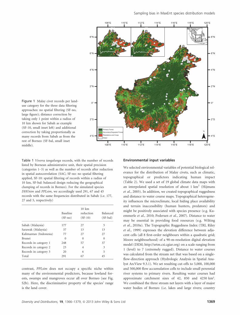
Figure 1 Malay civet records per land-

use category for the three data filtering

approaches: no spatial filtering (SF-no,

large figure); distance correction by

taking only 1 point within a radius of

10 km shown for Sabah as example

(SF-10, small inset left) and additional

correction by taking proportionally as

many records from Sabah as from the

rest of Borneo (SF-bal, small inset

middle).

Table 1 Viverra tangalunga records, with the number of records

listed by Bornean administrative unit, their spatial precision

(categories 1–3) as well as the number of records after reduction

in spatial autocorrelation (SAC; SF-no: no spatial filtering

applied, SF-10: spatial filtering of records within a radius of

10 km, SF-bal: balanced design reducing the geographical

clumping of records in Borneo). For the simulated species

DHOsim and PPLsim, we accordingly used 291, 67 and 45

records with the same frequencies distributed in Sabah (i.e. 177,

27 and 5, respectively)

Baseline

(SF-no)

10 km

reduction

(SF-10)

Balanced

(SF-bal)

Sabah (Malaysia) 177 27 5

Sarawak (Malaysia) 37 13 13

Kalimantan (Indonesia) 77 27 27

Brunei 0 0 0

Records in category 1 248 57 37



Total 291 67 45



inland water data of the Digital Chart of the World, www.

diva-gis.org) to create three ‘distance to water’ maps. For land

cover, we used the 50-m-resolution PALSAR land-cover map

validated for Borneo (Hoekman et al., 2009) from 2007 and

updated it with DEM data in 500-m elevation steps to obtain a

finer grain of land-cover classification, that is, forest cover was

classed into four different categories of lowland, upland, lower

montane and upper montane forests, as these classes might be

differently influenced by climate, human disturbance and rug-

gedness. The reclassified land-cover map had the following 17

land-cover classes: (1) lowland forest 0–500 m; (2) upland for-

est 501–1000 m; (3) lower montane forest 1001–1500 m; (4)

upper montane forest > 1500 m; (5) forest mosaics and frag-

mented or degraded forests 0–500 m; (6) forest mosaics and

fragmented or degraded forests 501–1000 m; (7) forest mosa-

ics and fragmented or degraded forests 1001–1500 m; (8) for-

est mosaics and fragmented or degraded forests > 1500 m; (9)

swamp forest; (10) mangrove; (11) old plantations; (12) young

plantations and crops; (13) burnt forest area; (14) mixed

crops; (15) water and fishponds; (16) water bodies; (17) no

data. Human population density data (LandScan 2007TM High

Resolution Global Population Data Set, Oak Ridge National

Laboratory, UT-Battelle, LLC) were also included, because

human presence may negatively impact carnivore presence

through forest fragmentation, disturbance and hunting (e.g.

Morueta-Holme et al., 2010).

Model scenarios

We generated systematic scenarios of species distribution

predictions by a stepwise combination of all possible options

specified below; that is, by spatial filtering and background

manipulation (SF and BM), we had three possibilities of

filtering or creating background files resulting in nine differ-

ent scenarios. These scenarios were repeated for the Malay

civet and the two simulated species. In addition, the two

options (SF and BM) were tested with the full set of environ-

mental input layers as well as a reduced number of uncorre-

lated input layers for the real dataset of the Malay civet,

resulting in 18 scenarios (cf. also results Table 3).

Option 1: Spatial filtering (SF)

We systematically assessed the consequences of spatial clump-

ing by first only using one record within a radius of 10 km

(Table 1, 10-km reduction scenario [SF-10]). This radius was

chosen because the mean home range size of individual Malay

civets is between 1 and 1.5 km2 (Colon, 2002; Jennings et al.,

2010), but home ranges were larger in logged forest compared

with primary forest (Colon, 2002). To account for different-

sized home ranges in different habitats and to ensure spatial

independence, we used a conservative approach with 10 km.

We retained the location with the greatest precision. Nonethe-

less, owing to the higher number of field studies from Sabah

compared with other Bornean regions, records were still heav-

ily geographically unbalanced, with Sabah containing > 50%

of all records despite covering only about 10% of the area of

Borneo. In a second stage, we thus further reduced the number

of records in Sabah by randomly selecting records to produce

a sample with the same density as outside of Sabah. As only 40

records were detected outside of Sabah (678,200 km²), we

included only five from Sabah (� 73,600 km²; Table 1,

balanced scenario [SF-bal]).

Option 2: Background manipulation with bias files (BM)

Generally, the background area for all scenarios was Borneo

(Fig. 1). We manipulated the background sampling effort with

two alternative species-specific ‘bias files’ representing the rela-

tive sampling effort or record density. Species records were

mapped on a 1-km² grid, and each cell was given a value of 1 if

it contained a record. We subsequently summed the number

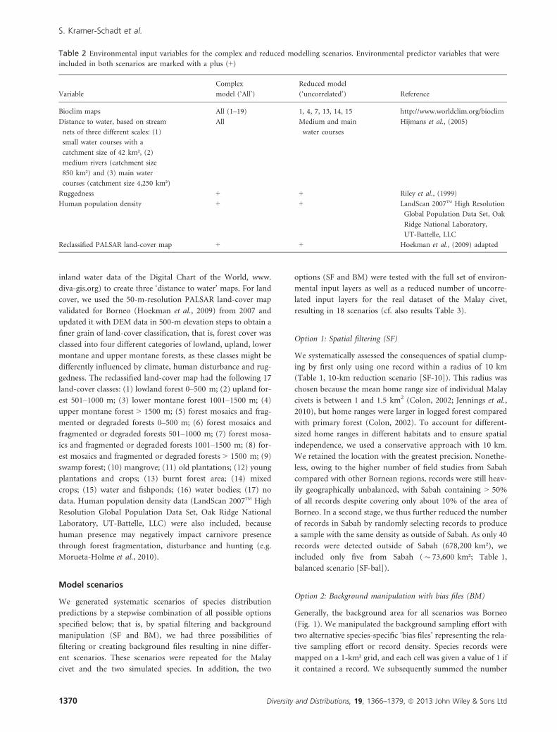
Table 2 Environmental input variables for the complex and reduced modelling scenarios. Environmental predictor variables that were

included in both scenarios are marked with a plus (+)

Variable

Complex

model (‘All’)

Reduced model

(‘uncorrelated’) Reference

Bioclim maps All (1–19) 1, 4, 7, 13, 14, 15 http://www.worldclim.org/bioclim

Distance to water, based on stream

nets of three different scales: (1)

small water courses with a

catchment size of 42 km², (2)

medium rivers (catchment size

850 km²) and (3) main water

courses (catchment size 4,250 km²)

All Medium and main

water courses

Hijmans et al., (2005)

Ruggedness + + Riley et al., (1999)

Human population density + + LandScan 2007TM High Resolution

Global Population Data Set, Oak

Ridge National Laboratory,

UT-Battelle, LLC

Reclassified PALSAR land-cover map + + Hoekman et al., (2009) adapted



Table

3OutcomeoftheMaxEntdistributionmodellingscenariosfortheMalay

civet(see

TableS3

forthesimulateddataDHOsim

andPPLsim).SF-no:nospatialfilteringapplied;SF-10:

reductionofrecordsin

aradiusof10

km;SF-bal:balanceddesign(see

maintext).BM-no:nobackgroundmanipulation,that

is,nobiasfile

used;BM-0.1:biasfile

with0.1backgroundfor

areaswithoutrecords.BM-0.01:

biasfile

with0.01

backgroundforareaswithoutrecords.Themodel

scenario

initalicswas

thebaselinescenario.

Modelledscenarios

ModelAUCs

Presence

thresholdsused

%Areaabove

threshold

Spatialfiltering(option1)

No.points

Backgroundmanipulationwithbiasfile(option2)

No.param

eters

TrainingAUC

TestAUC

10P

MTP

ETS

>0.5*

>10P

>MTP

>ETS

SF-no

291

BM-no

All

0.95

0.91

0.18

0.03

0.19

2.61

13.44

51.26

12.62

SF-10

67BM-no

All

0.88

0.74

0.26

0.13

0.17

8.8

33.33

56.33

47.96

SF-bal

45BM-no

All

0.86

0.67

0.41

0.12

0.22

18.21

30.21

75.35

57.82

SF-no

291

BM-0.1

All

0.94

0.90

0.47

0.13

0.4

11.32

13.35

59.82

19.2

SF-10

67BM-0.1

All

0.87

0.74

0.35

0.2

0.21

14.54

32.6

56.13

54.33

SF-bal

45BM-0.1

All

0.86

0.67

0.45

0.15

0.25

20.92

28.15

74.16

57.82

SF-no

291

BM-0.01

All

0.88

0.85

0.51

0.27

0.52

26.38

24.78

66.91

23.16

SF-10

67BM-0.01

All

0.85

0.74

0.47

0.36

0.37

27.77

33.68

55.29

53.36

SF-bal

45BM-0.01

All

0.82

0.67

0.48

0.25

0.39

30.03

34.4

75.18

52.25

SF-no

291

BM-no

Uncorrelated

0.92

0.87

0.16

0.04

0.21

3.37

27.13

6319.13

SF-10

67BM-no

Uncorrelated

0.83

0.69

0.25

0.14

0.21

10.42

48.53

69.15

56.44

SF-bal

45BM-no

Uncorrelated

0.83

0.64

0.43

0.08

0.26

22.16

33.62

90.03

61.19

SF-no

291

BM-0.1

Uncorrelated

0.92

0.87

0.42

0.21

0.42

13.82

24.78

61.96

24.78

SF-10

67BM-0.1

Uncorrelated

0.83

0.69

0.32

0.2

0.26

16.31

48.12

68.64

59.17

SF-bal

45BM-0.1

Uncorrelated

0.82

0.65

0.45

0.1

0.28

24.37

33.17

89.35

61.52

SF-no

291

BM-0.01

Uncorrelated

0.84

0.80

0.48

0.33

0.53

31.74

37.96

73.12

23.38

SF-10

67BM-0.01

Uncorrelated

0.82

0.70

0.45

0.33

0.38

31.61

45.86

70.77

61.62

SF-bal

45BM-0.01

Uncorrelated

0.79

0.65

0.47

0.2

0.37

32.64

40.31

87.36

61.79

*Fixed

threshold;MTP,minim

um

trainingpresence

logistic

threshold;10P,10th

percentile

trainingpresence

logistic

threshold;ETS,

equal

testsensitivity

andspecificity

logistic

threshold.



of records across the Moore neighbourhood of each cell to

produce a map of ‘sampling’ density. We used this width-

restricted moving window approach to ensure that only those

cells were included in the bias files where we were absolutely

sure that the species was sampled. If there was no record, a cell

was assigned the value 0.1, indicating a tenth of the sampling

effort of a value of 1 (bias scenario BM-0.1; see Fig. S1). We

further assessed the sensitivity of bias files by assigning values

of 0.01 to cells with no records (bias scenario BM-0.01) to

yield a scenario closer to non-sampling. Scenarios without

background manipulation were termed BM-no.

Reducing multicollinearity

As an alternative to a complex model including all environ-

mental variables (‘all’ scenario), we produced a reduced

version by eliminating correlating variables where Pearson’s

|r | > 0.75 (e.g. Dormann et al., 2012; Syfert et al., 2013)

(see Table S1). We retained the variable with the most cor-

relations with the other variables. This resulted in the inclu-

sion of only six climatic variables and two water maps

(Table 2, ‘uncorrelated’ scenario).

MaxEnt modelling and model evaluation

We ran MaxEnt version 3.3.3a (www.cs.princeton.edu/~schapire/

maxent; Phillips et al., 2006) with default settings as follows: ran-

dom test percentage = 25; regularization multiplier = 1; maxi-

mum number of background points = 10,000. We ran 10

replicates and used mean relative occurrence or suitability proba-

bilities predicted for further analyses. As measures of SDM accu-

racy or discriminative power, respectively, we used the

threshold-independent area under the curve (AUC) of the

receiver operating characteristic (ROC) plot (Fielding & Bell,

1997) produced by MaxEnt. Models with an AUC > 0.7 have

good discriminatory power (Hosmer & Lemeshow, 1989).

To aid model validation and interpretation and to check

for robustness of results, we compared four commonly used

MaxEnt thresholds to define the percentage of suitable habi-

tat (Liu et al., 2005; Jimenez-Valverde & Lobo, 2007): (1)

MaxEnt relative suitability probability > 0.5 as a fixed

threshold approach corresponding to a temporal and spatial

scale of sampling that results in a 50% chance of the species

being present in suitable areas (Elith et al., 2011), that is,

unlike true prevalence (Warton & Shepherd, 2010; Dorazio,

2012), (2) the minimum training presence logistic threshold

(MTP), (3) a 10th percentile training presence logistic

threshold (10P) and (4) an equal test sensitivity and specific-

ity logistic threshold (ETS).

We then selected three scenarios for model validation

(baseline: no background manipulation and no spatial filter-

ing [SF-no BM-no], only background manipulation: bias file

with 0.01 background but no spatial filtering [SF-no

BM-0.01] or a balanced design: no background manipula-

tion, but with spatial filtering [SF-bal BM-no]). In these

three scenarios, we assessed which scenario under-repre-

sented non-sampled areas (omission error or false negative,

that is, suitable area not correctly predicted) or overpredict-

ed the species range (commission error or false positive, that

is, wrongly predicted area that actually is not suitable). For

the field records of the Malay civet, we used the following

approach to evaluate model accuracy: To assess omission

error, we counted how many of the 67 records used in the

10-km reduction approach (Table 1) occurred in non-pre-

dicted areas separated by the widely used 10P threshold. We

could not assess commission errors without independent test

data; therefore, we used the predicted areas (10P threshold)

that occurred within oil palm plantations (reportedly unsuit-

able; Jennings et al., 2010) (land-cover classes 11 and 12, cf.

chapter ‘Environmental input variables’) as an optimistic

indicator of commission error. As an independent validation

of model accuracy, we used the simulated dataset where the

suitable range was predefined. Hence, the omission error is

the area defined as suitable but not predicted by the model.

In contrast, commission error is the predicted area that is

not suitable for the species (see Fig. S2).

RESULTS

Model scenarios

Option 1: Spatial filtering

Use of the full dataset for the Malay civet resulted in a strong

geographical clustering of predictions for areas (in our case

Sabah) where most records originated, that is, Sabah was

assigned the highest suitability (Fig. 2a–c; SF-no scenarios),

independent of the threshold used. Spatial filtering of the data-

set (SF-10 and SF-bal) resulted in greater representation of

non-surveyed areas outside Sabah (Fig. 2a–c). The degree of

increase in area predicted as suitable differed depending on

thresholds used: balancing the sampling design (SF-bal) dou-

bled the estimated suitable area for the 10P (from � 13% to

� 30%) and tripled the area for the ETS (from � 13% to

� 58%) threshold. The use of the predictive map with a fixed

threshold > 0.5 increased the estimated suitable area from

� 3% to 18%. Test AUCs were considerably reduced

(AUCs < 0.7) when using spatial filtering (Table 3); however,

the relative gain contribution (i.e. a goodness-of-fit measure)

of the most important variable increased (see Table S2). The

same results hold for the two simulated species (Tables S2 and

S3, Fig. S3). However, the AUC of the range-restricted species

DHOsim did not decrease with spatial filtering, which is due to

the narrow response range within the environmental predic-

tors (Table S3).

Option 2: Background manipulation with bias files

As with spatial filtering, background manipulation increased

the predicted distribution area for the Malay civet

independent of thresholds, but only if very low values (0.01)

were assigned to non-sampled areas (Table 3, Fig. 2a–c).



With background values of 0.1, the change in area predicted

was < 10% for all thresholds. The impact of bias files was

reduced in 10-km reduction scenarios, and background

manipulation almost had no further effect on balanced

model outcomes (Fig. 2, Table 3). Test AUCs were constant

(BM-0.1) or only slightly reduced by � 5% (BM-0.01,

Table 3). Using bias files also put more emphasis on the

explanatory power of single variables, that is, the relative

gain contribution increased (see Table S2). We observed the

same trend for the two simulated species (Tables S2 and S3,

Fig. S3).

Reducing multicollinearity

In contrast to the large effect of spatial filtering of records

on modelling results, we observed only minor differences

when correlated input variables were eliminated; differences

in predicted suitable habitat were slightly greater (2–5%) in

the reduced than the complex scenarios (Table 3, Fig. 2a–c

right side). These minor deviations were consistent across all

scenarios. Only in the models without spatial filtering

(SF-no) with the 10P threshold did the predicted distribution

area increase substantially (12–14%) in the parsimonious

scenario (Table 3 and Fig. 2b). In contrast, the predicted

suitable habitat in the balanced models [SF-bal] with the 10P

threshold appeared robust in terms of model complexity

(3–6%). In general, we observed a small decrease in AUC

values in parsimonious scenarios compared with complex

scenarios (2–5%). Due to reduction in environmental input

layers, the relative gain of the most important input variables

also increased (see Table S2).

In summary, spatial filtering, background manipulation

and reducing multicollinearity all increased the area predicted

as suitable habitat for the Malay Civet in Borneo as well as for

the simulated species. The choice of thresholds to define the

percentage of suitable habitat also heavily influenced model

results. However, the variation in important environmental

predictors was small, with only three predictors consistently

being the most important for 18 scenarios. Using a balanced

design consistently resulted in the same environmental predic-

tors (Table S2), indicating the robustness of this approach. In

the simulations of the range-restricted species DHOsim, the

underlying variable ‘land cover’ was never chosen as the most

important one due to the correlation of highland forest with

other environmental predictors. In contrast, PPLsim simula-

tions always revealed land cover as the most important one.

Model evaluation

Malay civet

Using the 67 occurrence records falling within the predicted

distribution area of the 10P threshold maps of the baseline

scenario (SF-no BM-no; Fig. 3a) and background manipula-

tion scenario with 0.01 bias file (SF-10 BM-0.01; Fig. 3b)

revealed very low omission errors for Sabah, the area with

(a) 50% fixed threshold‘All’ (complex) ‘Uncorrelated’ (pared down)BM-no BM-0.01 BM-no BM-0.01

[SF-no]

[SF-10]

[SF-bal]

10P threshold‘All’ (complex) ‘Uncorrelated’ (pared down)BM-no BM-0.01 BM-no BM-0.01

[SF-no]

[SF-10]

[SF-bal]

MTPthreshold‘All’ (complex) ‘Uncorrelated’ (pared down)BM-no BM-0.01 BM-no BM-0.01

[SF-no]

[SF-10]

[SF-bal]

(b)

(c)

Figure 2 MaxEnt spatial predictions for the Malay civet for

different scenarios of data filtering [SF-no, SF-10, SF-bal],

background manipulations [BM-no, BM-0.01], thresholds used

to separate the map into binary predictions (suitable: black

colour, unsuitable: grey colour) (a–c) and for varying model

complexity (left or right columns) (see Fig. S3 for simulated

datasets DHOsim and PPLsim).



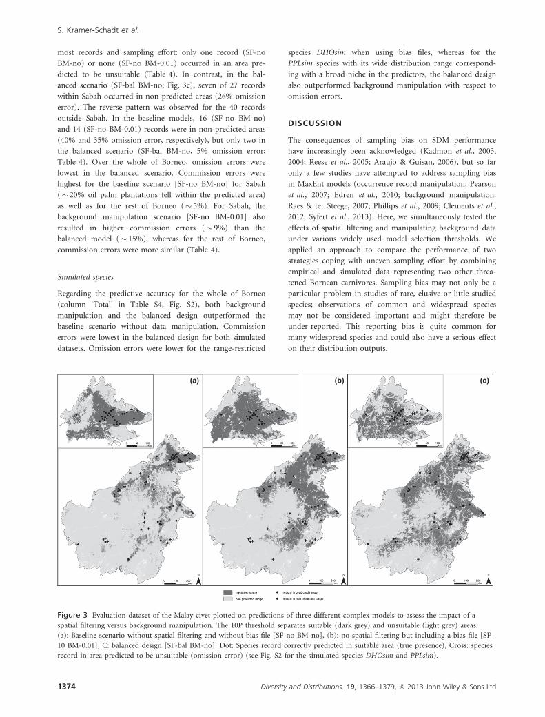
most records and sampling effort: only one record (SF-no

BM-no) or none (SF-no BM-0.01) occurred in an area pre-

dicted to be unsuitable (Table 4). In contrast, in the bal-

anced scenario (SF-bal BM-no; Fig. 3c), seven of 27 records

within Sabah occurred in non-predicted areas (26% omission

error). The reverse pattern was observed for the 40 records

outside Sabah. In the baseline models, 16 (SF-no BM-no)

and 14 (SF-no BM-0.01) records were in non-predicted areas

(40% and 35% omission error, respectively), but only two in

the balanced scenario (SF-bal BM-no, 5% omission error;

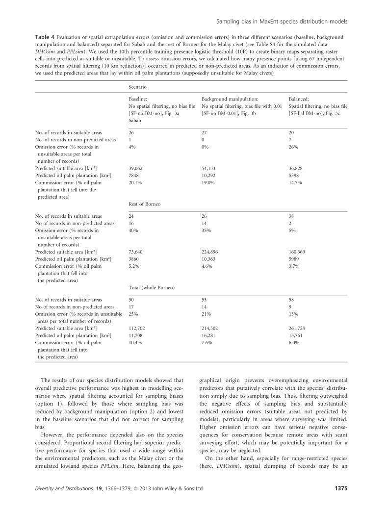
Table 4). Over the whole of Borneo, omission errors were

lowest in the balanced scenario. Commission errors were

highest for the baseline scenario [SF-no BM-no] for Sabah

(� 20% oil palm plantations fell within the predicted area)

as well as for the rest of Borneo (� 5%). For Sabah, the

background manipulation scenario [SF-no BM-0.01] also

resulted in higher commission errors (� 9%) than the

balanced model (� 15%), whereas for the rest of Borneo,

commission errors were more similar (Table 4).

Simulated species

Regarding the predictive accuracy for the whole of Borneo

(column ‘Total’ in Table S4, Fig. S2), both background

manipulation and the balanced design outperformed the

baseline scenario without data manipulation. Commission

errors were lowest in the balanced design for both simulated

datasets. Omission errors were lower for the range-restricted

species DHOsim when using bias files, whereas for the

PPLsim species with its wide distribution range correspond-

ing with a broad niche in the predictors, the balanced design

also outperformed background manipulation with respect to

omission errors.

DISCUSSION

The consequences of sampling bias on SDM performance

have increasingly been acknowledged (Kadmon et al., 2003,

2004; Reese et al., 2005; Araujo & Guisan, 2006), but so far

only a few studies have attempted to address sampling bias

in MaxEnt models (occurrence record manipulation: Pearson

et al., 2007; Edren et al., 2010; background manipulation:

Raes & ter Steege, 2007; Phillips et al., 2009; Clements et al.,

2012; Syfert et al., 2013). Here, we simultaneously tested the

effects of spatial filtering and manipulating background data

under various widely used model selection thresholds. We

applied an approach to compare the performance of two

strategies coping with uneven sampling effort by combining

empirical and simulated data representing two other threa-

tened Bornean carnivores. Sampling bias may not only be a

particular problem in studies of rare, elusive or little studied

species; observations of common and widespread species

may not be considered important and might therefore be

under-reported. This reporting bias is quite common for

many widespread species and could also have a serious effect

on their distribution outputs.

(a) (b) (c)

Figure 3 Evaluation dataset of the Malay civet plotted on predictions of three different complex models to assess the impact of a

spatial filtering versus background manipulation. The 10P threshold separates suitable (dark grey) and unsuitable (light grey) areas.

(a): Baseline scenario without spatial filtering and without bias file [SF-no BM-no], (b): no spatial filtering but including a bias file [SF-

10 BM-0.01], C: balanced design [SF-bal BM-no]. Dot: Species record correctly predicted in suitable area (true presence), Cross: species

record in area predicted to be unsuitable (omission error) (see Fig. S2 for the simulated species DHOsim and PPLsim).



The results of our species distribution models showed that

overall predictive performance was highest in modelling sce-

narios where spatial filtering accounted for sampling biases

(option 1), followed by those where sampling bias was

reduced by background manipulation (option 2) and lowest

in the baseline scenarios that did not correct for sampling

bias.

However, the performance depended also on the species

considered. Proportional record filtering had superior predic-

tive performance for species that used a wide range within

the environmental predictors, such as the Malay civet or the

simulated lowland species PPLsim. Here, balancing the geo-

graphical origin prevents overemphasizing environmental

predictors that putatively correlate with the species’ distribu-

tion simply due to sampling bias. Thus, filtering outweighed

the negative effects of sampling bias and substantially

reduced omission errors (suitable areas not predicted by

models), particularly in areas where surveying was limited.

Higher omission errors can have serious negative conse-

quences for conservation because remote areas with scant

surveying effort, which may be potentially important for a

species, may be neglected.

On the other hand, especially for range-restricted species

(here, DHOsim), spatial clumping of records may be an

Table 4 Evaluation of spatial extrapolation errors (omission and commission errors) in three different scenarios (baseline, background

manipulation and balanced) separated for Sabah and the rest of Borneo for the Malay civet (see Table S4 for the simulated data

DHOsim and PPLsim). We used the 10th percentile training presence logistic threshold (10P) to create binary maps separating raster

cells into predicted as suitable or unsuitable. To assess omission errors, we calculated how many presence points [using 67 independent

records from spatial filtering (10 km reduction)] occurred in predicted or non-predicted areas. As an indicator of commission errors,

we used the predicted areas that lay within oil palm plantations (supposedly unsuitable for Malay civets)

Scenario

Baseline: Background manipulation: Balanced:

No spatial filtering, no bias file No spatial filtering, bias file with 0.01 Spatial filtering, no bias file

[SF-no BM-no]; Fig. 3a [SF-no BM-0.01]; Fig. 3b [SF-bal BM-no]; Fig. 3c

Sabah

No. of records in suitable areas 26 27 20

No. of records in non-predicted areas 1 0 7

Omission error (% records in

unsuitable areas per total

number of records)

4% 0% 26%

Predicted suitable area [km²] 39,062 54,133 36,828

Predicted oil palm plantation [km²] 7848 10,292 5398

Commission error (% oil palm

plantation that fell into the

predicted area)

20.1% 19.0% 14.7%

Rest of Borneo


No of records in non-predicted areas 16 14 2

Omission error (% records in

unsuitable areas per total

number of records)

40% 35% 5%


Predicted oil palm plantation [km²] 3860 10,363 5989


plantation that fell into

the predicted area)

5.2% 4.6% 3.7%

Total (whole Borneo)


No of records in non-predicted areas 17 14 9

Omission error (% records in unsuitable

areas per total number of records)

25% 21% 13%


Predicted oil palm plantation [km²] 11,708 16,281 15,761


plantation that fell into

the predicted area)

10.4% 7.6% 6.0%



ecological signal (Dormann et al., 2007), and filtering the

records can weaken the prediction; in these cases, it would

be preferable to use a bias file. However, this implies prior

knowledge about the species’ distribution, which often is not

available. In the case of the Malay civet, use of a bias file

resulted in higher commission errors (areas mistakenly pre-

dicted to be suitable): Only a few records existed from oil

palm plantations (all in close vicinity to forests; cf. Jennings

et al., 2010), and thus, plantations were downweighted by

the bias files to rarely sampled areas, equally in and outside

Sabah. However, the concentration of records in Sabah led

to greater weight on distinct climatic variables such that oil

palm plantations in Sabah were predicted to be more suitable

than those outside Sabah. Commission errors may have par-

ticular negative consequences because they can create the

false assumption that a species occurs in protected areas or

intact habitat, potentially leading to parts of its range being

ignored by conservation efforts.

Our results clearly highlight that spatial filtering of

clumped records (balanced scenario) minimized both omis-

sion and commission errors for Borneo-wide predictions and

was robust in regard to consistently identifying the most

important predictor. Thus, accounting for sampling bias is

needed, and a conservative approach (balanced design) is

recommended, despite the putatively lower predictive perfor-

mance according to the test AUC values. It is worth men-

tioning that as a consequence of reducing the number of

input records to achieve a balanced design, the predictive

power of the model is reduced (Hernandez et al., 2006). In

this respect, the most commonly used metric for model qual-

ity (test AUC) can be misleading (Lobo et al., 2007) and can

poorly represent the underlying biology of the system being

studied (Warren & Seifert, 2011).

Another argument for recommending a balanced design,

rather than only background manipulation, is the arbitrary

values that have to be set for bias files and the arbitrary way

in which they are created when only presence records are

available. It is exactly the putative advantage of MaxEnt in

comparison with presence–absence or occupancy models that

redounds to its disadvantage when used without caution.

The values in the bias file (cf. see Option 2: Background

manipulation with bias files (BM) in the methods section)

have to match sampling effort, which is difficult to estimate

when dealing with records stemming from different spatio-

temporal scales or occasional sightings. Often, the distribu-

tion of records is set as a proxy for sampling effort. For

example, for the Malayan tapir Tapirus indicus, Clements

et al. (2012) used a weighted Gaussian distance kernel based

on presence records and tapir’s home range size and scaled

their bias file between 1 (non- or undersampled areas) and

100 (clumped presence records). We used a next-neighbour

approach assuming higher sampling effort around records,

resulting in at least ten (background value 0.1) or 100 (back-

ground value 0.01) times less sampling effort in non- or

undersampled areas. The comparison between our two back-

ground value scenarios (Table 3) showed that the arbitrary

estimate for sampling effort influenced model results. There

is scope to improve the precision with which bias files reflect

sampling effort, for example, by accounting for trap nights if

the records come predominantly from camera-trapping stud-

ies. However, when a dataset is composed of opportunistic

sightings and road kills alongside structured sampling (e.g.

typically from scientific studies), as investigations of little

known species typically are, it is effectively impossible to

obtain objective values for sampling effort in different areas.

We recommend further investigations of the effect of differ-

ently created bias files.

Increased model complexity may lead to overfitting, which

involves using too many environmental input variables with

too few occurrence records. For example, Warren & Seifert

(2011) found that overparameterization is generally less prob-

lematic than underparameterization. The exception occurred

when model complexity (in terms of the number of environ-

mental input variables) approached or exceeded the number

of records available for model construction, in which case less

complex models performed better (see also Reineking &

Schr€oder, 2006). In this study, we evaluated the impact of

model complexity and showed that the area predicted as suit-

able was less affected if occurrence records were spatially inde-

pendent and stratified throughout the area of inference

(balanced model). In contrast, the baseline model predictions

were more sensitive to model complexity, and bias in occur-

rence predictions increased with model complexity.

The selection of a threshold for assessing areas of poten-

tially suitable habitat is another crucial aspect of the assess-

ment of the output of SDMs (Liu et al., 2005) and is needed

for any model application, for example, in conservation. We

used several thresholds to assess whether spatial autocorrela-

tion of occurrence records, based on uneven sampling, was a

problem independent of the specific threshold selected.

Although great differences were observed in the percentage

of area predicted to be suitable, the overall effect was consis-

tent for all thresholds; that is, areas with a proportionally

greater number of records were overpredicted, and non-sur-

veyed areas were underpredicted, particularly if no correction

of sampling bias was applied (baseline models).

CONCLUSIONS

We recommend that in situations with a strong sampling

bias towards some regions or environmental features (e.g.

survey and therefore records mainly distributed in a certain

land-cover type), spatial clumping of records should be

reduced in datasets that are used for MaxEnt model calibra-

tion. If many occurrence records are available, our results

demonstrate that spatial filtering and balancing of occurrence

data are preferred relative to background manipulation. If

only few spatially clustered occurrence records are available

and spatial filtering is impossible, the manipulation of the

background dataset seems to be the second best option.

Background manipulation decreased the risk of omission

errors for the range-restricted species occupying a narrow



niche within many environmental predictors, but increased it

for the species with a generalist response in many predictors;

therefore, any conclusions regarding areas suitable for con-

servation ought to be made with caution. Our study

acknowledges the potential of MaxEnt as a powerful tool in

SDM and highlights the importance of accounting for sam-

pling bias to help reduce omission and commission errors

and thus enhances the accuracy of species conservation and

management.

ACKNOWLEDGEMENTS

We thank Gabriella Fredriksson, Jedediah Brodie, William

J. McShea, Tim van Berkel and the Heart of Borneo Pro-

ject, Rob Stuebing and Deni Wahyudi of the REA KalTim

Conservation Department for providing Malay Civet records

used for this study. Ana Rodrigues gave useful advice on

omission and commission errors. We thank Manuela

Fischer for support in the final GIS analyses. Further, we

thank all participants of the 1st Borneo Carnivore Sympo-

sium (BCS) 2011, Kota Kinabalu, Sabah, Malaysia, for the

insightful discussions on and after the symposium. We are

indebted to the Sabah Wildlife Department to co-organize

the BCS together with the Cat-, Small Carnivore- and

Otter-IUCN/SSC Specialist Groups and the Leibniz Institute

for Zoo and Wildlife Research. Financial support for the

BCS was provided by the following institutions: Benta Wa-

wasan Sdn Bhd; British Ecological Society; Chester Zoo –

The North England Zoological Society; Cleveland Metro-

parks; The Clouded Leopard Project; Columbus Zoo;

Department of Wildlife, Fisheries and Aquaculture, Flora

Blossom Sdn Bhd; Forest and Wildlife Research Center,

Mississippi State University; Houston Zoo; KTS Plantation

Sdn Bhd; Leibniz Institute for Zoo and Wildlife Research;

Malaysia Airlines; Nashville Zoo; Point Defiance Zoo and

Aquarium; Shared Earth Foundation; The Usitawi Network;

Wild Cat Club; WWF-Germany; WWF-Malaysia. DWM,

AJH and JR warmly acknowledge the support of the Reca-

nati-Kaplan Foundation and the Woodspring Trust.

REFERENCES

Araujo, M.B. & Guisan, A. (2006) Five (or so) challenges for

species distribution modelling. Journal of Biogeography, 33,

1677–1688.

Augeri, D.M.. 2005. On the biogeographic ecology of the Mala-

yan sun bear. Ph.D. Dissertation. School of Biological Sci-

ences, University of Cambridge, Cambridge, UK. 330 pp.

Baasch, D.M., Tyre, A.J., Millspaugh, J.J., Hygnstrom, S.E. &

Vercauterenm, K.C. (2010) An evaluation of three statisti-

cal methods used to model resource selection. Ecological

Modelling, 221, 565–574.

Bateman, B.L., VanDerWal, J. & Johnson, C.N. (2011) Nice

weather for bettongs: using weather events, not climate

means, in species distribution models. Ecography, 35, 306–

314.

Brodie, J. & Giordano, A. (2011) Small carnivores of the

Maliau Basin, Sabah, Borneo, including a new locality for

Hose’s Civet Diplogale hosei. Small Carnivore Conservation,

44, 1–6.

Clements, G.R., Rayan, D.M., Aziz, S.A., Kawanishi, K., Trae-

holt, C., Magintatn, D., Yazi, M.F.A. & Tingley, R. (2012)

Predicting the distribution of the Asian Tapir (Tapirus in-

dicus) in Peninsular Malaysia using maximum entropy

modelling. Integrative Zoology, 7, 400–406.

Colon, C.P. (2002) Ranging behaviour and activity of the

Malay civet (Viverra tangalunga) in a logged and an un-

logged forest in Danum Valley, East Malaysia. Journal of

Zoology, 257, 473–485.

Dorazio, R.M. (2012) Predicting the geographic distribution

of a species from presence-only data subject to detection

errors. Biometrics, 68, 1303–1312.

Dormann, C.F., McPherson, J.M., Araujo, M.B., Bivand,

R., Bolliger, J., Carl, G., Davies, R.G., Hirzel, A., Jetz, W.,

Kissling, W.D., Kuehn, I., Ohlemueller, R., Peres-Neto,

P.R., Reineking, B., Schroeder, B., Schurr, F.M. & Wilson,

R. (2007) Methods to account for spatial autocorrelation

in the analysis of species distributional data: a review.

Ecography, 30, 609–628.

Dormann, C.F., Elith, J., Bacher, S., Buchmann, C., Carl, G.,

Carre, G., Garcia Marquez, J.R., Gruber, B., Lafoourcade,

B., Leitao, P.J., M€unkem€uller, T., Mcclean, C., Osborne,

P.E., Reineking, B., Schr€oder, B., Skidmore, A.K., Zurell,

D. & Lautenbach, S. (2012) Collinearity: a review of meth-

ods to deal with it and a simulation study evaluating their

performance. Ecography, 35, 1–20.

Edren, S.M.C., Wisz, M.S., Teilmann, J., Dietz, R. & S€oderk-

vist, T. (2010) Modelling spatial patterns in harbour

porpoise satellite telemetry data using maximum entropy.

Ecography, 33, 698–708.

Elith, J. & Leathwick, J.R. (2009) Species distribution models:

ecological explanation and prediction across space and time.

Annual Review of Ecology and Systematics, 40, 677–697.

Elith, J., Graham, C.H., Anderson, R.P. et al. (2006) Novel

methods improve prediction of species’ distributions from

occurrence data. Ecography, 29, 129–151.

Elith, J., Phillips, S., Hastie, T., Dudik, M., Chee, Y.E. &

Yates, C.J. (2011) A statistical explanation of MaxEnt for

ecologists. Diversity and Distributions, 17, 43–57.

Fielding, A.H. & Bell, J.F. (1997) A review of methods for the

assessment of prediction errors in conservation presence/

absence models. Environmental Conservation, 24, 38–49.

Franklin, J. (2009) Mapping species distributions. spatial

inference and prediction. Cambridge University Press, New

York.

Graham, C.H., Elith, H.J., Hijmans, R.J., Guisan, A., Peter-

son, A.T., Loiselle, B.A. & The NCEAS Predicting Species

Distributions Working Group (2008) The influence of spa-

tial errors in species occurrence data used in distribution

models. Journal of Applied Ecology, 45, 239–247.

G€uthlin, D., Knauer, F., Kneib, T., K€uchenhoff, H., Kaczen-

sky, P., Rauer, G., Jonozovic, M., Mustoni, A. & Jerina, K.



(2011) Estimating habitat suitability and potential popula-

tion size for brown bears in the Eastern Alps. Biological

Conservation, 144, 1733–1741.

Hernandez, P.A., Graham, C.H., Master, L.L. & Albert, D.L.

(2006) The effect of sample size and species characteristics

on performance of different species distribution modeling

methods. Ecography, 29, 773–785.

Hijmans, R.J., Cameron, S.E., Parra, J.L., Jones, P.G. & Jarvis,

A. (2005) Very high resolution interpolated climate sur-

faces for global land areas. International Journal of Clima-

tology, 25, 1965–1978.

Hoekman, D., Vissers, M. & Wielaard, N. (2009) PALSAR

land cover mapping methodology validation study Borneo.

Wageningen University, The Netherlands. pp. 1–112.

Hosmer, D.W. & Lemeshow, S. (1989) Applied logistic regres-

sion. Wiley, New York.

Hu, J. & Jiang, Z. (2011) Climate change hastens the conser-

vation urgency of an endangered ungulate. PLoS ONE, 6,

e22873.

Jennings, A.P. & Veron, G. (2011) Predicted distributions

and ecological niches of 8 civet and mongoose species in

Southeast Asia. Journal of Mammalogy, 92, 316–327.

Jennings, A.P., Zubaid, A. & Veron, G. (2010) Ranging

behaviour, activity, habitat use, and morphology of the

Malay civet (Viverra tangalunga) on Peninsular Malaysia

and comparison with studies on Borneo and Sulawesi.

Mammalian Biology, 75, 437–446.

Jimenez-Valverde, A. & Lobo, J.M. (2007) Threshold criteria

for conversion of probability of species presence to either–

or presence–absence. Acta Oecologica, 31, 361–369.

Kadmon, R., Farber, O. & Danin, A. (2003) A systematic

analysis of factors affecting the performance of climatic

envelope models. Ecological Applications, 13, 853–867.

Kadmon, R., Farber, O. & Danin, A. (2004) Effect of road-

side bias on the accuracy of predictive maps produced by

bioclimatic models. Ecological Applications, 14, 401–413.

Kalkvik, H.M., Stout, I.J., Doonan, T.J. & Parkinson, C.L.

(2011) Investigating niche and lineage diversification in

widely distributed taxa: phylogeography and ecological

niche modeling of the Peromyscus maniculatus species

group. Ecography, 34, 1–11.

Kremen, C., Cameron, A., Moilanen, A. et al. (2008) Align-

ing conservation priorities across taxa in Madagascar with

high-resolution planning tools. Science, 320, 222–226.

K€uhn, I. (2007) Incorporating spatial autocorrelation may

invert observed patterns. Diversity and Distributions, 13,

66–69.

Kuemmerle, T., Perzanowski, K., Chaskovskyy, O., Ostapowicz,

K., Halada, L., Bashta, A.-T., Kruhlov, I., Hostert, P., Waller,

D.M. & Radeloff, V.C. (2010) European Bison habitat in the

Carpathian Mountains. Biological Conservation, 143, 908–

916.

Li, W. & Guo, Q.E.C. (2011) Can we model the probability

of presence of species without absence data? Ecography, 34,

1096–1105.

Liu, C., Berry, P.M., Dawson, T.P. & Pearson, R.G. (2005)

Selecting thresholds of occurrence in the prediction of spe-

cies distributions. Ecography, 28, 385–393.

Lobo, J.M., Jimenez-Valverde, A. & Real, R. (2007) AUC: a

misleading measure of the performance of predictive distri-

bution models. Global Ecology & Biogeography, 17, 145–

151.

MacKenzie, D.I. (2005) What are the issues with presence-

absence data for wildlife managers? Journal of Wildlife

Management, 63, 849–860.

Morueta-Holme, N., Flojgaard, C. & Svenning, J.C. (2010)

Climate change risks and conservation implications for a

threatened small-range mammal species. PLoS ONE, 5,

e10360.

Pearson, R.G., Raxworthy, C.J., Nakamura, M. & Peterson,

A.T. (2007) Predicting species distributions from small

numbers of occurrence records: a test case using cryptic

geckos in Madagascar. Journal of Biogeography, 34,

102–117.

Pedersen, A.O., Jepsen, J.U., Yoccoz, N.G. & Fuglei, E.

(2007) Climate Change Risks and Conservation Implica-

tions for a Threatened Small-Range Mammal Species.

Canadian Journal of Zoology, 85, 122–132.

Phillips, S.J. (2008) Transferability, sample selection bias and

background data in presence-only modelling: a response to

Peterson et al. (2007). Ecography, 31, 272–278.

Phillips, S.J., Anderson, R.P. & Schapire, R.E. (2006) Maxi-

mum entropy modeling of species geographic distributions.

Ecological Modelling, 190, 231–259.

Phillips, S.J., Dudik, M., Elith, J., Graham, C.H., Lehmann,

A., Leathwick, J. & Ferrier, S. (2009) Sample selection bias

and presence-only distribution models: implications for

background and pseudo-absence data. Ecological Applica-

tions, 19, 181–197.

Raes, N. & ter Steege, H. (2007) A null-model for signifi-

cance testing of presence-only species distribution models.

Ecography, 30, 727–736.

Reddy, S. & Davalos, L.M. (2003) Geographical sampling

bias and its implications for conservation priorities in

Africa. Journal of Biogeography, 30, 1719–1727.

Reese, G.C., Wilson, K.R., Hoeting, J.A. & Flather, C.H.

(2005) Factors affecting species distribution predictions: a

simulation modeling experiment. Ecological Applications,

15, 554–564.

Reineking, B. & Schr€oder, B. (2006) Constrain to perform:

regularization of habitat models. Ecological Modelling, 193,

675–690.

Renner, I.W. & Warton, D.I. (2013) Equivalence of MAX-

ENT and poisson point process models for species distri-

bution modeling in ecology. Biometrics, 69, 274–281.

Riley, S.J., De Gloria, S.D. & Elliot, R. (1999) A terrain

ruggedness that quantifies topographic heterogeneity.

Intermountain Journal of Science, 5, 23–27.

Rondinini, C., Wilson, K.A., Boitani, L., Grantham, H. &

Possingham, H.P. (2006) Tradeoffs of different types of



species occurrence data for use in systematic conservation

planning. Ecology Letters, 9, 1145.

Royle, J.A., Chandler, R.B., Yackulic, C. & Nichols, J.D.

(2012) Likelihood analysis of species occurrence probability

from presence-only data for modelling species distribu-

tions. Methods in Ecology and Evolution, 3, 545–554.

Ruiz-Gutierrez, V. & Zipkin, E.F. (2011) Detection

biases yield misleading patterns of species persistence

and colonization in fragmented landscapes. Ecosphere,

2, 1–14.

Sastre, P. & Lobo, J.M. (2009) Taxonomist survey biases and

the unveiling of biodiversity patterns. Biological Conserva-

tion, 142, 462–467.

Syfert, M.M., Smith, M.J. & Coomes, D.A. (2013) The effects

of sampling bias and model complexity on the predictive

performance of MaxEnt species distribution models. PLoS

ONE, 8, e55158.

Veloz, S.D. (2009) Spatially autocorrelated sampling falsely

inflates measures of accuracy for presence-only niche

models. Journal of Biogeography, 36, 2290–2299.

Warren, D.L. & Seifert, S.N. (2011) Ecological niche model-

ing in Maxent: the importance of model complexity and

the performance of model selection criteria. Ecological

Applications, 21, 335–342.

Warton, D.I. & Shepherd, L.C. (2010) Poisson point process

models solve the “pseudo-absence problem” for presence-

only data in ecology. The Annals of Applied Statistics, 4,

1383–1402.

Wilting, A., Cord, A., Hearn, A.J., Hesse, D., Mohamed, A.,

Traeholdt, C., Cheyne, S.M., Sunarto, S., Jayasilan, M.-A.,

Ross, J., Shapiro, A.C., Sebastian, A., Dech, S., Breitenmo-

ser, C., Sanderson, J., Duckworth, J.W. & Hofer, H.

(2010a) Modelling the species distribution of flat-headed

cats (Prionailurus planiceps), an endangered South-East

Asian small felid. PLoS ONE, 5, e9612.

Wilting, A., Samejima, H. & Mohamed, A. (2010b) Diversity

of Bornean viverrids and other small carnivores in Dera-

makot Forests Reserve, Sabah, Malaysia. Small Carnivore

Conservation, 42, 10–13.

Wisz, M.S., Hijmans, R.J., Li, J., Peterson, A.T., Graham,

C.H., Guisan, A. & The NCEAS Predicting Species Distri-

butions Working Group (2008) Effects of sample size on

the performance of species distribution models. Diversity

and Distribution, 14, 763–773.

Yackulic, C.B., Chandler, R., Zipkin, E.F., Royle, J.A.,

Nichols, J.D., Campbell Grant, E.H. & Veran, S. (2013)

Presence-only modelling using MAXENT: when can we

trust the inferences? Methods in Ecology and Evolution, 4,

236–243.

SUPPORTING INFORMATION

Additional Supporting Information may be found in the

online version of this article:

Table S1 Pearson’s product–moment correlation r matrix of

environmental input layers.

Table S2. Three most important variables and their relative

contributions (%) of the environmental variables to the

MaxEnt models.

Table S3. Outcome of the MaxEnt distribution models for

the simulated data DHOsim and PPLsim.

Table S4. Evaluation of spatial extrapolation errors (omis-

sion and commission errors) in three different scenarios

(baseline, background manipulation and balanced) for the

simulated data (DHOsim and PPLsim) separated for Sabah

and the rest of Borneo.

Figure S1. Example of bias file.

Figure S2. Predefined suitable areas of (a) a range-restricted

species occurring in mountainous forests (DHOsim) and (b)

a lowland species dwelling in peat swamps, mangroves and

lowland forests (PPLsim).

Figure S3. MaxEnt spatial predictions of the simulated

datasets DHOsim and PPLsim for the different scenarios.

BIOSKETCH

All authors of this manuscript are interested in the distribu-

tion and conservation of Bornean carnivores and in the

application of species distribution modelling as a tool to

improve the efficiency of conservation planning.

Authors’ contributions: S.K-S and A.W. conceived the ideas,

led the analysis and wrote the paper. J.N., J.L., V.R., M.L.,

I.H., B.S. and A.K.S. helped to perform the modelling and

GIS analyses. J.D.P., D.M.A., S.M.C., A.J.H., J.R, D.W.M.,

J.M., J.E., A.J.M., G.S., R.R., H.B., R.A., H.S., J.W.D., C.B-W.,

J.L.B. and H.H contributed to data collection and revised the

final manuscript.

Editor: Mark Robertson



The importance of correcting for sampling bias in MaxEnt species ...

Documents

Transcript of The importance of correcting for sampling bias in MaxEnt species ...