The Implied Futures Financing Rate∗

Nicholas L. Gunther† Robert M. Anderson‡ Lisa R. Goldberg§

Alex Papanicolau¶

February 20, 2021

∗We thank our present and former colleagues at the Center for Risk Management Research and theConsortium for Data Analytics in Risk for many interesting and stimulating discussions that enhanced thequality of this article.

†Department of Economics and Consortium for Data Analytics in Risk, University of California at Berke-ley, nlgunther@berkeley.edu.

‡Department of Economics and Consortium for Data Analytics in Risk, University of California at Berke-ley, robert.anderson@berkeley.edu.

§Departments of Economics and Statistics and Consortium for Data Analytics in Risk¶Consortium for Data Analytics in Risk, University of California at Berkeley,

1

Contents

1 Introduction. 3

2 Literature 4

3 Interest Rates Implied by Futures 5

3.1 General Case without Dividends . . . . . . . . . . . . . . . . . . . . . . . . . 5

3.2 The Expected Discount and the IFFR . . . . . . . . . . . . . . . . . . . . . 9

3.3 General Case with Dividends . . . . . . . . . . . . . . . . . . . . . . . . . . . 11

4 The Model of Stock and Interest Rates 13

4.1 Specification . . . . . . . . . . . . . . . . . . . . . . . . . . . . . . . . . . . . 14

4.2 Preliminary Results for Later Use . . . . . . . . . . . . . . . . . . . . . . . . 14

4.3 Canonical Coordinates for Brownian Diagonalization . . . . . . . . . . . . . 16

5 Estimating the Model 18

5.1 Objective and Methodology for Model Estimation . . . . . . . . . . . . . . . 18

5.2 Estimating (σr)2 . . . . . . . . . . . . . . . . . . . . . . . . . . . . . . . . . 20

5.3 Is the Estimate σ2|d Reasonable? . . . . . . . . . . . . . . . . . . . . . . . . 25

5.4 Estimating σS, ρ . . . . . . . . . . . . . . . . . . . . . . . . . . . . . . . . . . 26

5.5 Estimating the Convexity Adjustment . . . . . . . . . . . . . . . . . . . . . 30

6 Spread Analysis 31

7 Summary 34

1

The Implied Futures Financing Rate

Abstract

We explore the cost of implicit leverage associated with an S&P 500 Index futures contract

and derive an implied financing rate (the Futures-Implied Rate or FIR), based on a simple

model of stock and futures, without any explicit arbitrage or other relationship to market

interest rates. We develop new estimation methods for the FIR, including point and interval

estimates, with important advantages over existing methods, and extend our methods to

bivariate estimates of the FIR and equity volatility based on Wishart distributions. While our

resulting FIR estimates were often attractive relative to market rates on explicit financings,

the relationship between the implicit and explicit financing rates was volatile and varied

considerably based on legal and economic regimes. Among our significant findings was the

effectiveness of regulatory reform in reducing substantially the spreads between this FIR and

contemporaneous LIBOR and US Treasury rates. Other findings include estimates of the

convexity adjustment associated with the FIR, futures-based estimates of stock volatility

and stock-rate correlation, and new test statistics for the significance of these estimates.

2

1 Introduction.

What is the true financing cost of a levered equity investment strategy? Generally speaking,

an investor who wishes more exposure than her free cash permits has two choices: she can

borrow and add the debt proceeds to her cash investment, or, as discussed in this article,

she can obtain implicit leverage through the derivatives market.1 In this paper, we explore

the cost of implicit leverage associated with a prominent equity index futures contract. In

summary, our research shows that the related implicit financing rate has often been attractive

relative to market rates on explicit financing; however, the relationship between the implicit

and explicit financing rates has been volatile and varied considerably based on legal and

economic regimes.

The purchase of an S&P 500 Index2 futures contract3 results in exposure to a notional

amount of the underlying in exchange for a current payment much less than that notional

amount.4 Intuitively, this suggests financing; a levered purchase of the underlying equities

provides similar exposure and cash flows. In this paper, we consider a stock and two futures

contracts on the stock, from which we derive an implied forward financing rate (the futures

implied rate, or FIR). This rate represents the implicit cost of financing associated with

such an investment in a futures contract. The spread between this implied rate and market

interest rates evolved dynamically over a series of four regimes that we identified during

our total observation period from January 1996 to June 2019. The Commodity Futures

Modernization Act of 2000 (“CFMA”) reduced this spread; the 2008 financial crisis and the

subsequent recovery each altered it further.

1For an exploration of explicit leverage, see, e.g., Anderson et al. (2014).2The term ‘S&P 500 Index’ is a registered copyright of Standard & Poors, Inc.3Unless otherwise stated, the terms futures contract in this article refers to such an S&P 500 Index futures

contract. The terms of such futures contracts are specified by the Chicago Mercantile Exchange (CME ) forthe big (or floor) and the small (or E-mini) futures contracts traded through the CME. Current terms forsuch futures contracts are available on the CME’s website. The CME has other futures contracts relatedto the S&P 500 Index, including contracts that reflect dividends on the index components. These othercontracts lack the volume and the history of the traditional contract we choose.

4The payment required to execute a futures contract consists principally of initial and variational margin;leverage of 10:1 or higher is often possible. See footnote 3.

3

We begin our investigation of the FIR with few restrictions on the stock and futures price

processes, and then for more explicit results specialize to a simple model of stock and futures,

without any explicit arbitrage or other relationship to market interest rates.

2 Literature

The futures literature is extensive5 and the relationship between futures prices and interest

rates is well-studied in the customary context of no-arbitrage pricing.6 There is however,

little on that relationship outside that no-arbitrage context, where market rates and rates

implied by futures can be unequal.7 Recently, recognition that simple static models of

futures hedges are inadequate has appeared.8 Our current article investigates the interest

rate implied by S&P 500 futures prices determined independently from market interest rates,

to our knowledge for the first time.9

Anderson et al. (2014) analyze the cost of explicit financing in a levered equity investment

strategy; the current article provides a companion analysis of the cost of implicit financing.

5Dating back at least to, e.g., Black (1976).6See, e.g., Cox et al. (1981) (showing, inter alia, that futures and forward prices are equal if rates are

deterministic.)7For example, because, unlike forward contracts, as a result of variational margin (see footnote 4), hedges

between positions in the underlying physical stock and in futures contracts are dynamic and thus leaveresidual open risk.

8Contrast Dwyer et al. (1996) (using a simple static cost of carry model to explore the nonlinear relation-ship between the S&P 500 Futures and the underlying stock) with Hilliard et al. (2021) (using a ’short-livedarbitrage’ model proposed in (Otto, 2000) to compute minimum variance hedge ratios.)

9The futures literature discusses many other topics not relevant to the current investigation. See,e.g., Chen et al. (2016) (comparing price discovery in futures, index options and ETFs) and referencescited therein; Chan et al. (1991) (comparing volatility in the cash and index futures markets); Bali et al.(2008)(testing mean reversion in S&P 500 futures) and Lien (2004)(investigating the effect of cointegrationon hedging effectiveness.)

4

3 Interest Rates Implied by Futures

3.1 General Case without Dividends

The basic equations for futures and implied financing rates used in this paper come from the

well-known no-arbitrage relationship that relates the futures price F (t, T ) at the current time

t to the expected stock price S(T ) at the maturity date T of the relevant futures contract,

conditioned on the information at time t:

Theorem 3.1. Futures as Expectation

F (t, T ) = Et[S(T )] ≡ EQ[S(T )|t] ≡ EQ[S(T )|Ft] (1)

This result is true quite generally, independent of any particular model for the stock or

interest rates. The Computational Appendix contains a proof in continuous time.10

In Equation (1), EQ[S(T )|Ft] denotes the expectation of S(T) conditional on the informa-

tion available at an earlier time t under the risk neutral measure Q associated with riskless

investment in a money market account we denote by M(t0, t1), t0 < t1. We will assume there

is a short rate process r(t) associated with this riskless investment. The related (stochastic)

discount factor (or just discount) is also denoted by M but with time order reversed:

M(t0, t1) = e∫ t1t0r(s)ds, M(t1, t0) =

1

M(t0, t1)

We assume that rt is attainable11 from the stock, the near futures contract and the next

futures contract on the S&P 500 Index.12 Such a short rate process need not be equivalent to

10For a proof in the discrete case, see, e.g., (Anderson and Kercheval, 2010, Chapter 4).11A claim is attainable from other claims if there is a self-financing trading strategy in those other claims

that has the same payoffs as the first claim. See, e.g. (Anderson and Kercheval, 2010, Chapter 2.3).12These contracts are traded on the Chicago Mercantile Exchange. In market terminology, the near

contract is the one with the earliest possible maturity after the observation time, and the next contract isthe one with next earliest maturity. The difference in the maturity dates of two consecutive S&P 500 Indexfutures contracts, such as the near and the next, is typically approximately three months. In this research,

5

a market interest rate, where two rates are equivalent if they may be swapped into each other

at no cost.13 Instead, it is the rate of riskless investment attainable through a self-financing

portfolio in the stock and the futures, and as such represents the FIR.

We assume there is no arbitrage and, at first, also that S pays no dividends. Accord-

ingly S(t) equals its expected discounted future value under the standard Martingale Pricing

Formula (MPF ):14

S(t) = Et[S(T )M(T, t)], T > t (2)

Using this and the well-known relationship between the covariance and the expectation of

a product of two random variables, the inverse futures ratio (IFR) is given by:

IFR ≡ S(t)

F (t, T )=Et[S(T )M(T, t)]

F (t, T )

=Et[S(T )]Et [M(T, t)]

F (t, T )+

covt (S(T ),M(T, t))

F (t, T )(3)

= Et [M(T, t)] +covt (S(T ),M(T, t))

Et[S(T )](4)

= Et [M(T, t)] + covt

(S(T )

Et[S(T )],M(T, t)

)(5)

= Et [M(T, t)]

(1 + covt

(S(T

Et[S(T )],

M(T, t)

Et [M(T, t)]

))(6)

Equation (4) follows from Equation (3) by Equation (1). Equation (5) follows from Equation

we have used the big or floor contract because of its longer existence; in later years the volume of the E-miniis typically larger but the closing prices are almost always the same.

13Two equivalent rates are said in the market to have a zero basis between them. ‘Equivalence’ in thissense requires a static hedge, so that each rate is attainable from the other in a very simple way using marketinstruments. Compare Footnote 11 above. In the absence of arbitrage, two equivalent rates should differ bytheir credit risk, and as a result of variational margin and other credit mitigation features the risk associatedwith futures is extremely low. Were the FIR and a market rate equivalent, one would expect the FIR totrack closely the risk-free rate. Figure (1) does not support such equivalence.

14The MPF states that the current price of a security or other self-financing trading strategy equals theconditional expectation of its discounted future cash flows, including its terminal future value, discountingby the riskless investment or other numeraire. (Anderson and Kercheval, 2010, Chapter 3). In the absenceof dividends, the terminal future value is the only future cash flow, as in the equation in the text.

6

(4) since Et[S(T )] is known at time t. Finally, Equation (6) follows because Et [M(T, t)] is

also known at time t.

The IFR is the ratio of the current stock price to the futures price and thus measures

the discount implied by the futures. Equation (5) says simply that this measure equals the

expected discount plus a covariance term. The first term on the right in Equation (5) is the

expected term discount factor over [t, T ], corresponding to the FIR. The final term on the

right in Equation (5) equals the covariance of the stock price and the FIR discount factor at

time T around their expected values, viewed from time t.

It is instructive to compare Equation (5) with the analogous equation for a fair forward

contract with forward price ≡ Fo(t, T ). Since the price of a fair forward contract should be

zero, we have from the MPF:

S(t) = Fo(t, T )Et[M(T, t)]

or equivalently,

S(t)

Fo(t, T )= Et[M(T, t)] (7)

Comparing Equations (5), (6) and (7) and recalling the definition of the IFR, we see that

the covariance term may be thought of as a convexity adjustment.15

For empirical reasons,16 it is easier to work with two futures contracts, the near and the

15Lacking a covariance term, the determination of an implied financing rate from a forward appearssuperficially more appealing than the more complex determination from a futures contract. More basically,an equity forward on a stock has two cash flows: a current fixed cash payment and a future equity-linkedpayment on the notional amount at maturity. Because there are only two cash flows, the forward-impliedfinancing rate can be directly observed. By contrast, a futures contract has daily, often substantial cashflows in respect of variational margin, in effect marking the contract to market daily. Therefore determiningthe associated implied financing rate requires financial theory, as Equation (5) demonstrates. However, forcredit and other reasons, forwards are OTC, not exchange traded, illiquid and bespoke, and so the contractterms, from which financing rates could be directly observed, are private and not fungible.

16These reasons include high price volatility, asynchronicity between the close of the cash and the futuresmarkets, market segmentation and the substantial volume of daily transactions in both the spot and the

7

next,17 and the inverse forward futures ratio than the inverse futures ratio itself. We will

also need the forward discount M(T2, T1). We define the inverse forward futures ratio or

IFFR by:

IFFR ≡ F (t, T2, T1) ≡ F (t, T1)

F (t, T2),

where T2 > T1 are the maturities of the next and the near futures, respectively, and the final

quotient is the near contract futures price divided by the next contract futures price, in each

case observed at time t.

In this article, generally consistent with our data, we assume that

∆T ≡ T2 − T1 = 0.25 (A1)

T2 ≤ 0.5 (A2)

We measure time in years, so ∆T = 0.25 of one year, or one-quarter.18 By Assumption (A1),

Assumption (A2) is equivalent to assuming T1 ≤ 0.25.

futures markets. See generally Anderson et al. (2013). A more detailed description of our methodologyappears in the Computational Appendix.

17See Footnote 12 above.18Id. These assumptions come from the approximately quarterly calendar of futures contracts.

8

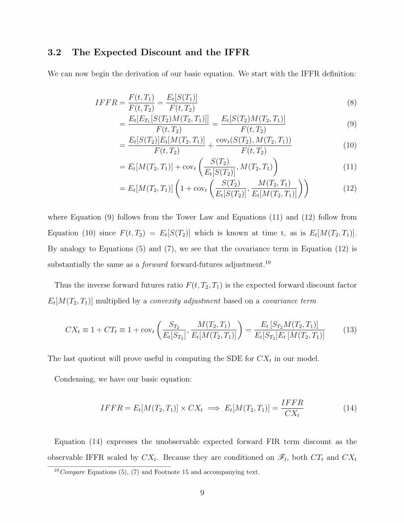
3.2 The Expected Discount and the IFFR

We can now begin the derivation of our basic equation. We start with the IFFR definition:

IFFR =F (t, T1)

F (t, T2)=Et[S(T1)]

F (t, T2)(8)

=Et[ET1 [S(T2)M(T2, T1)]]

F (t, T2)=Et[S(T2)M(T2, T1)]

F (t, T2)(9)

=Et[S(T2)]Et[M(T2, T1)]

F (t, T2)+

covt(S(T2),M(T2, T1))

F (t, T2)(10)

= Et[M(T2, T1)] + covt

(S(T2)

Et[S(T2)],M(T2, T1)

)(11)

= Et[M(T2, T1)]

(1 + covt

(S(T2)

Et[S(T2)],

M(T2, T1)

Et[M(T2, T1)]

))(12)

where Equation (9) follows from the Tower Law and Equations (11) and (12) follow from

Equation (10) since F (t, T2) = Et[S(T2)] which is known at time t, as is Et[M(T2, T1)].

By analogy to Equations (5) and (7), we see that the covariance term in Equation (12) is

substantially the same as a forward forward-futures adjustment.19

Thus the inverse forward futures ratio F (t, T2, T1) is the expected forward discount factor

Et[M(T2, T1)] multiplied by a convexity adjustment based on a covariance term

CXt ≡ 1 + CTt ≡ 1 + covt

(ST2

Et[ST2 ],

M(T2, T1)

Et[M(T2, T1)]

)=

Et [ST2M(T2, T1)]

Et[ST2 ]Et [M(T2, T1)](13)

The last quotient will prove useful in computing the SDE for CXt in our model.

Condensing, we have our basic equation:

IFFR = Et[M(T2, T1)]× CXt =⇒ Et[M(T2, T1)] =IFFR

CXt

(14)

Equation (14) expresses the unobservable expected forward FIR term discount as the

observable IFFR scaled by CXt. Because they are conditioned on Ft, both CTt and CXt

19Compare Equations (5), (7) and Footnote 15 and accompanying text.

9

are deterministic functions of t determined by the unknown parameters of the processes

M and S.

While S and IFRR are both observable,20 M is not, and therefore CXt is also unobservable.

Equation (14) thus expresses the unobservable (expected) FIR on the left-hand side in terms

of the unobservable CXt on the right-hand side, which also depends on the unobservable

M(T2, T1). The unobservable M(T2, T1) therefore appears on both sides of Equation (14),

creating an apparent circularity in the estimation expression we wish to use - to use Equation

(14) to estimate the FIR that appears by itself on the left-hand side, we must already know

it to determine the denominator (= CXt) on Equation (14)’s right-hand side.

Were these quantities simply unknown numbers, standard algebra might provide a solu-

tion, but instead they are time-dependent and determined from an unobservable stochastic

quantity (M(T2, T1)) with unknown parameters. In Section 5.5 below, we develop a new

calculus to resolve this circularity and provide an explicit estimate of CXt based on our

model.

CXt’s Effect Should be Insignificant We sketch a rough argument that on our data,

the effect of CXt is likely to be small and thus Et[M(T2, T1)] should equal the IFFR with

modest error. We then preview our later result that this error is in fact insignificant outside

a small minority of periods, making the FIR directly observable as a practical matter, with

negligible error. See Figures (7) and (8).

20But only imperfectly. The S&P 500 is the hypothetical portfolio of stocks underlying an index, observingwhich raises asynchronicity and other issues. For example, the index at each instant in time is a weightedaverage of the most recent trade prices of the constituent stocks. Since the S&P 500 stocks are relativelylarge and liquid, on most days there will be at least one trade of most or all of the stocks, but there maybe days on which some stocks do not trade at all, in which case the price information would be stale byat least 24 hours. The more common situation in these relatively large stocks is that the last trade occursseveral minutes or even several hours before the close; for example, there are occasional trading halts inspecific stocks. For different stocks, the time of the last trade may therefore differ. For another example,trading does not actually stop at the nominal close (4 pm). At the close, there will be some limit orders andbuy/sell on close orders that remain to be executed. These orders are crossed, with trading times up to tenminutes after the close. To that extent the closing price of each of the individual constituent stocks may notbe known at the close. See, e.g., Anderson et al. (2013)

10

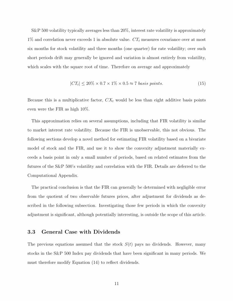
S&P 500 volatility typically averages less than 20%, interest rate volatility is approximately

1% and correlation never exceeds 1 in absolute value. CTt measures covariance over at most

six months for stock volatility and three months (one quarter) for rate volatility; over such

short periods drift may generally be ignored and variation is almost entirely from volatility,

which scales with the square root of time. Therefore on average and approximately

|CTt| ≤ 20%× 0.7× 1%× 0.5 ≈ 7 basis points. (15)

Because this is a multiplicative factor, CXt would be less than eight additive basis points

even were the FIR as high 10%.

This approximation relies on several assumptions, including that FIR volatility is similar

to market interest rate volatility. Because the FIR is unobservable, this not obvious. The

following sections develop a novel method for estimating FIR volatility based on a bivariate

model of stock and the FIR, and use it to show the convexity adjustment materially ex-

ceeds a basis point in only a small number of periods, based on related estimates from the

futures of the S&P 500’s volatility and correlation with the FIR. Details are deferred to the

Computational Appendix.

The practical conclusion is that the FIR can generally be determined with negligible error

from the quotient of two observable futures prices, after adjustment for dividends as de-

scribed in the following subsection. Investigating those few periods in which the convexity

adjustment is significant, although potentially interesting, is outside the scope of this article.

3.3 General Case with Dividends

The previous equations assumed that the stock S(t) pays no dividends. However, many

stocks in the S&P 500 Index pay dividends that have been significant in many periods. We

must therefore modify Equation (14) to reflect dividends.

11

We obtained implied dividend rates rdiv(t) on the S&P 500 from the option markets, based

on put-call parity.21 As derived in the Computational Appendix,22 the required modification

to Equation (14) is:

Et[M(T2, T1)] =kdiv(t)× IFFR

CXt

. (16)

where23

kdiv(t) = 1− rdiv(t)∆T.

The value kdiv(t) lies between 0 and 1.24 Thus in the presence of dividends the left-hand

side of Equation (14) decreases by kdiv(t). As a result of this formula, we can include the

effect of dividends by applying to the IFFR a discount of kdiv(t) (or equivalently increasing

the forward futures ratio by 1kdiv(t)

) and then computing as though there were no dividends.

Equation (16) can be written in identical form to Equation (14) if we replace IFFR with

kdiv(t) × IFFR; except where explicitly otherwise indicated, we will do so hereafter to

simplify notation.

Figure (1) shows the FIR determined from the IFFR as described at the end of Section 3.2,

adjusted for dividends but not convexity, expressed as a rate and appropriately annualized.

This graph, with US Treasury and LIBOR rates included for comparison, provides informal,

visual confirmation that the FIR behaves similarly to market interest rates, although it is

not equivalent to any of them. A more precise statement requires the model in the following

section.

21Wharton Research Data Services’ OptionMetrics contains a time series of estimated implied dividendrates rdiv(t) obtained from a regression with the property that the present value at time t of the implieddividends over (t, T ] equals rdiv(t)× S(t)× (T − t), where S(t) is the price of the associated stock at time t.See Ivy DB File and Data Reference Manual 30, Version 3.0, revised May 19, 2011.

22Computational Appendix [?? ??].23Time is measured in full years, so a six-month interval measures 0.5.24Since (1) ∆T is on the order of a quarter and (2) dividend rates on the S&P 500 have always been

positive but less than 400% (an extremely high rate).

12

4 The Model of Stock and Interest Rates

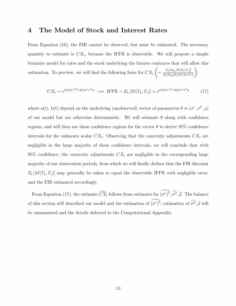
From Equation (16), the FIR cannot be observed, but must be estimated. The necessary

quantity to estimate is CXt, because the IFFR is observable. We will propose a simple

bivariate model for rates and the stock underlying the futures contracts that will allow this

estimation. To preview, we will find the following form for CXt

(=

Et[ST2M(T2,T1)]Et[ST2 ]Et[M(T2,T1)]

):

CXt = ea(t)(σr)2+b(t)σrσSρ =⇒ IFFR = Et [M(T2, T1)]× ea(t)(σr)2+b(t)σrσSρ (17)

where a(t), b(t) depend on the underlying (unobserved) vector of parameters θ ≡ (σr, σS, ρ)

of our model but are otherwise deterministic. We will estimate θ along with confidence

regions, and will then use these confidence regions for the vector θ to derive 95% confidence

intervals for the unknown scalar CXt. Observing that the convexity adjustments CXt are

negligible in the large majority of these confidence intervals, we will conclude that with

95% confidence, the convexity adjustments CXt are negligible in the corresponding large

majority of our observation periods, from which we will finally deduce that the FIR discount

Et [M(T2, T1)] may generally be taken to equal the observable IFFR with negligible error,

and the FIR estimated accordingly.

From Equation (17), the estimate CXt follows from estimates for (σr)2, σS, ρ. The balance

of this section will described our model and the estimation of (σr)2; estimation of σS, ρ will

be summarized and the details deferred to the Computational Appendix.

13

4.1 Specification

We rely on a Ho-Lee interest rate model and a standard stock lognormal model. In matrix

form, it is

drtdStSt

=

µrdt+ σrdBrt

rtdt+ σSdBSt

(18)

with dBt ≡(dBS

t , dBrt

)a two-dimensional Brownian motion with instantaneous correlation

ρ and rt ≡ FIR(t). The parameters µr, σr, σS, ρ are all constant.

4.2 Preliminary Results for Later Use

Restricting to our model, we have the following useful technical propositions. The proofs

are deferred to the Computational Appendix.

Let F(t,T) denote the futures price at time t under a futures contract on the stock St with

expiration at time T.

Proposition: 4.1. Stock Price Evolution

S(T ) = Ste

∫ Tt

(rs−σ

S2

2

)ds+

∫ Tt σSBSs

(19)

The next proposition, which follows from the first and Theorem (3.1), describes the futures

price evolution in our model.

Proposition: 4.2. Futures SDE:

dF (t, T )

F (t, T )= (T − t)σrdBr

t + σSdBSt (20)

The third proposition describes the FIR discount evolution in our model.

14

Proposition: 4.3. FIR Discount Evolution

dEt [M(T2, T1)]

Et [M(T2, T1)])= (t ∨ T1 − T2)σrdBr

t , T2 ≥ T1, t (21)

From Proposition 4.3, consistent with one’s intuition, Et [M(T2, T1)] continues to evolve

for T1 < t < T2, but with diminishing volatility.

The final proposition provides the explicit formula for CXt discussed at the beginning of

this section.

Proposition: 4.4. Convexity Evolution

Et[M(T2, T1)ST2 ] = Et [M(T2, T1)]Et[ST2 ]eU1(T2,θ)−U2(t,θ)

where U1(T2, θ)− U2(t, θ)

=(σr)2

4

1

2

(1

48− (T2 − t)2

)− σr

4σSρ

(T1 − t+

1

8

)≡ a(t) (σr)2 + b(t)σrσSρ

Proposition 4.4 follows from Propositions (4.1) and (4.3). Details are deferred to the

Computational Appendix.

It will be helpful to express Proposition 4.4 as a quadratic form:

U1(T2, θ)− U2(t, θ) =

[σr ρσS

]Q(t)

σrρσS

(22)

Q(t) ≡

18

(148− (T2 − t)2

)18

(T1 − t+ 1

8

)18

(T1 − t+ 1

8

)0

15

The form Q is deterministic and can be computed once, independent of the particular

(next, near) pair of futures for which the convexity term is estimated.

4.3 Canonical Coordinates for Brownian Diagonalization

Let Fi, i = 1, 2 be two futures (a futures pair) on the stock St with sequential maturities

(expiration dates) T1 < T2. From Proposition 4.2:

dFiFi

= (Ti − t)σrdBr + σSdBs, i = 1, 2

We wish to diagonalize these two SDEs in terms of the bivariate Brownian motion dBt.

Using a change of variables to isolate the Brownian motion in terms of stochastically-

integrable quantities

X =logF2 − logF1

T2 − T1

,

Y =T2 − tT2 − T1

logF1 −T1 − tT2 − T1

logF2

Note that X = 1T2−T1 × log

(F2

F1

)and so functions as a proxy for the IFFR. X, Y are both

observable and have the following SDEs:

dXdY

=

σrdBr + dg(t; θ)

σSdBs + dh(t; θ) +Xdt

(23)

where θ = (σr, σS, ρ), dBrdBs = ρ and

g(t; θ) = −1

2

∫ t

0

{(T2 − s)2 − (T1 − s)2

T2 − T1

(σr)2 + 2σrσSρ

}ds,

h(t; θ) =1

2

∫ t

0

{(T2 − s)(T1 − s) (σr)2 ds− (σS)2

}ds

g, h are deterministic but depend on θ.

16

Integrating Equation (23), rearranging and using the approximation25

∫Xdt ≈ 1

2(Xt+∆t +Xt)∆t ≡ XAvg∆t

we may discretize Equation (23):

∆X

∆Y

=

σr∆Brt − (σr)2 (T1 − t)∆t

σS∆BSt +XAvg∆t− 1

2(σr)2 ∆t (t− T1)(t− T2))

+

[c

](24)

where c is a (vector) constant depending on θ.26

We rewrite Equation (24) in terms of the Brownian motion increments:

σr∆Brt

σS∆BSt

=

∆X + (σr)2 (T1 − t)∆t

∆Y −XAvg∆t+ 12

(σr)2 ∆t (t− T1)(t− T2))

+

[c

](25)

Equation (25) illustrates, in the context of our model, the circularity referred to in Section

3.2 above. If we knew the unknown parameter (σr)2 we could determine the right-hand

side, up to the unknown constant, detrending the observations of ∆X and ∆Y and leaving

a series of fully-observed iid samples of the bivariate Brownian increments on the left-hand

side. We could then estimate the covariance matrix of the left-hand side with the usual

methods. However, the parameter (σr)2 we need to estimate the covariance matrix in this

manner is itself one of the entries the covariance matrix we wish to estimate. The next

section describes the modification required to the usual methods to resolve this circularity.

25Since we observe both Xt+∆t, Xt, X is based on a Brownian Bridge. [The Computational Appendix pro-vides further justification for this approximation.]

26Herein ‘c’ denotes a constant, generally differing based on the context.

17

5 Estimating the Model

5.1 Objective and Methodology for Model Estimation

Objective. Our basic equation for the FIR is Equation (17). In that equation, the IFFR is

observed directly, but from Proposition 4.4 and Equation (22) the convexity adjustment that

multiplies the IFFR to determine the FIR discount depends on the two unknown quantities,

a variance and a covariance (σr)2 , σrσSρ, with the observed deterministic coefficients given

in Proposition 4.4.

Equation (1) relies on the absence of arbitrage, as does our model at certain other points,

so the relevant variance and covariance derive from the risk-neutral measure. Instead, we

estimate these quantities in the physical (real-world) measure, for two reasons. First, the

FIR is not directly observable and so the traditional Breeden-Litzenberger framework does

not extend naturally to provide from a schedule of prices for options on S&P 500 futures

contracts an estimate of the underlying bivariate stock-rate distribution.27 Second, more

practically, options on the S&P 500 futures are illiquid at many strikes28 rendering the

Breeden-Litzenberger estimates unreliable.

By contrast, the S&P 500 futures trade liquidly in substantial volume and so we have

based our estimates on their closing prices.29

To estimate confidence intervals for the FIR thus requires confidence regions for these

two quantities, over which we may take the maximum and minimum of Equation (22) to

determine a confidence interval for the convexity adjustment. We will see empirically that

27Cf. Equation (18). The Breeden-Litzenberger framework was first described in Breeden-Litzenberger(1978).

28For example, the CME Volume and Open Interest report on December 5, 2020 showed the averageclosing volume over available strikes of the Dec 20 puts was less than 2% of the volume for the underlyingfutures contract. The average volume for the Dec 20 calls was significantly less than that of the puts.

29Although implied and realized volatility of course differ from each other, the former has been viewed aspredicting the latter. See, e.g., Poon and Granger (2003). In this article, we are concerned primarily withaverage levels of volatility and covariance over substantial periods, over which the two may reasonably beviewed as approximate surrogates for each other.

18

outside a small minority of periods the convexity adjustment is negligible with 95% confidence

across all futures pairs and periods; therefore the FIR may be estimated directly from the

observed IFFR with a high degree of confidence.

In the final sections of this article, we will use these estimates over our entire observa-

tion period, more than two decades long, to identify the four regimes mentioned in the

introduction.

Methodology. We proceed by (i) estimating, for each period and corresponding futures

pair, an associated confidence region for the three parameters in θ, and then (ii) finding the

corresponding confidence interval for the convexity adjustment by maximizing and minimiz-

ing that adjustment over the confidence region for the period.

In the following subsection, we start by deriving, again for each period and corresponding

futures pair, a point and confidence interval estimate for the associated FIR variance ≡

(σr)2 in that period. In the ensuing subsections, we use that point estimate (σr)2 to de-

trend Equation (25) and estimate a two-dimensional confidence region for σS, ρ | (σr)2

conditional on that point estimate, as the dependence of the drift term in Equation (25)

on the unknown parameter (σr)2 suggests. We then use Equation (22) and the previously-

computed30 matrices Q(t) at each time to maximize and minimize the convexity adjustment

over that conditional confidence region, deriving a conditional confidence interval for the

convexity adjustment supporting the conclusion that, conditional on the estimate (σr)2, the

convexity adjustment is typically negligible over our entire observation period with similar

confidence.

In the Computational Appendix, we vary the estimates (σr)2 over a (σr)2 confidence inter-

val to estimate unconditional maxima and minima for the convexity adjustment and show

that, outside a few periods, it remains negligible with a high degree of confidence.

30See the final paragraph in Section 4.2 supra.

19

5.2 Estimating (σr)2

Throughout this subsection Na, Nq denote the observations per year and per quarter, gener-

ally around 248 and 62, respectively.

The first row of Equation (24) implies:

∆X ∈ N

((σr)2 (t− T1)∆t+ c1,

(σr)2

Na

)

To derive iid random variables for estimation, we rewrite this as

∆X + (σr)2 (T1 − t)∆t ∈ N

(c1,

(σr)2

Na

)(26)

Taking the unbiased sample variance of the left-hand side of Equation (26),

Na × s2(∆X + (σr)2 (T1 − t)∆t

)∈ (σr)2 χ2

f (27)

where we annualize based on Na observations per year. We estimate quarterly using Nq

observations =⇒ f ≡ Nq − 1 degrees of freedom for the estimated variance of these iid

normal random variables with unknown means.

Equation (27) exhibits the circularity problem described previously: to estimate the sample

variance of the iid samples in Equation (26), we first need to detrend the observable series

∆X, to do which requires the variance we’re trying to estimate.

To express this circularity in more conventional statistical terms, define the conditional

sample variance estimate by

s2a,f |σ2 ≡ Na

f× s2

(∆X + σ2(T1 − t)∆t

)(28)

20

s2a,f |σ2 is thus the ordinary annualized sample variance estimate31 after detrending the time

series ∆X using (conditional on) σ2, the true variance. s2a,f |σ2 is not a statistic because of

its dependence on the unknown σ2; however, a simple modification of the usual methods

nonetheless provides a solution.

To simplify the notation in the remainder of this section, we will dispense with the super-

script denoting the FIR variance and set σ2 ≡ (σr)2. We divide both sides of Equation (27)

by σ2 to get a draw d from a standard sampling distribution:

d(σ2) ≡f × s2

a,f |σ2

σ2∈ χ2

f (29)

Here, σ2 is the true variance and Equation (29) is a conventional frequentist statement about

repeated samples ∆X. Letting σ2 = σ20 be a particular null hypothesis about the value of

σ2, the right-hand side of Equation (29) becomes a test statistic in the usual way:

T (σ20) ≡ d(σ2

0) =f × s2

a,f |σ20

σ20

∈ χ2f (30)

Using the sampling distribution χ2f we can as usual determine critical regions for any sig-

nificance level α and the p-value of the observed test static T (σ20) but we do not have a

conventional point estimate σ2 and so cannot determine confidence intervals in the conven-

tional manner. We can only construct such a point estimate conditional on a null value σ20 to

use for detrending, another manifestation of the circularity referred to in Section 3.2 above.

We now derive point estimates in a novel manner, using a method related to fiducial

inference.32 Note that s2a,f |σ2

0 is the ordinary annualized sample variance estimate after

detrending the time series ∆X using (conditional on) a particular hypothesized null value

31The ‘a’ subscript denotes annualization and reflects multiplication by Na, and the ’f’ subscript denotesthe number of observations Nq − 1. Although we know the true mean is 0, there is an unknown constant inEquation (25) to be estimated, implying Nq − 1 degrees of freedom, by which we must divide to determinethe sample estimate.

32Fisher (1935).

21

σ20. As previously remarked, we do not in our context have a single sample variance estimate

Naf× s2(); rather we have a continuum of estimates s2

a,f |σ20, each conditional on a different

null value σ2 = σ20 used to detrend the observations.

Letting the variable uσ2 represent the possible null values σ20, we may view T : R++ → R++

as a function T (uσ2) of a positive real variable uσ2 . In the Computational Appendix, we show

that this function T (uσ2) has a restricted inverse33 uσ2(d) ≡ T −1(d) : [Tmin,∞) ⊂ R++ →

(0, uσ2,argmin] ⊂ R++ (these domain and range intervals are defined in the Computational

Appendix) mapping values d ∈ [Tmin,∞) of the test statistic bijectively to (possible) null

values in its range.34

We will assume, and confirm empirically, that the intervals [Tmin,∞), (0, uσ2,argmin] are

large enough, meaning that the latter interval is likely to contain any reasonable hypotheses

(σr0)2 consistent with our data. For example, f > Tmin in all cases on our data, as will be

important for the point estimate below.

The standard χ2f distribution for the test statistic has distinguished values (such as the

mean, the mode and quantiles) by virtue of being a distribution, and each such value d

in the domain of T −1 then corresponds to a particular null value uσ2(d) that in turn gives

rise as described below to a particular conditional sample variance estimate given the test

statistic value d, which we will shorten to conditional estimate, σ2|d ≡ uσ2(d).35 In general,

σ2|d 6= s2a,f |uσ2(d); the sample estimate typically differs from the true value in conventional

33As used herein : means “such that”.34One could find an approximate inverse for a given d from Equation (??) by simple trial-and-error. In

the Computational Appendix we derive a closed-form solution. To see that some restriction on T is needed,note that T → ∞ as σ2

0 → 0,∞. Thus, T () is not univalent, but since T > 0, T has a global minimum Tminattained by a (σr)

20,argmin. T is univalent above and below (σr)

20,argmin. There is no a priori measure on

null values σ20 ∈ R+, but we can induce one (a pull-back measure) in a standard way from the χ2

f distributionvia T , once restricted to be univalent, under which T will preserve measure by construction: the pull-backmeasure is the push-forward measure associated with T −1. Details are left to the Computational Appendix.

35The notation is intended to emphasize that, rather than starting with a null hypothesis σ20 , we start

with a draw d ∈ χ2f and then treat the associated null hypothesis uσ2(d) as an estimate corresponding to

d. The pull-back measure on null values from Footnote 34 provides further motivation for constructingthese estimates; under this measure T is measure-preserving by construction, and the significance levels ofconventional confidence intervals are determined by their pull-back measure in a natural way.

22

statistics, and the same is true in our context.

A Point Estimate. The mean of a χ2f variable is f, which treated as a draw d = f

from χ2f corresponds to the estimate σ2|f ≡ uσ2(f) ≡ T −1(f). From Equation (??) with

σ20 = uσ2(f), T (uσ2(f)) = f ⇐⇒ σ2|f ≡ uσ2(f) = s2

a,f |uσ2(f). Thus, the estimate σ2|f

corresponds to a conditional sample variance estimate s2a,f |uσ2(f) that itself equals that σ2|f ,

which we can therefore think of as a fixed point estimate. An equivalent description of this

fixed point estimate that generalizes well to the multivariate case is to think of it as the

zero error estimate, explained as follows. We may think of the quantitys2a,f |uσ2uσ2

− 1 as a

measure of the error (the null error)36 in our sample variance estimate s2a,f |uσ2 relative to a

hypothesized null value uσ2 .

In the conventional case where the sample variance estimate does not depend on the null

value and we have simply

∆X ∈ N

(c1,

(σr)2

Na

)=⇒ s2

a,f |uσ2 =Na

f× s2 (∆X) ≡ σ2

independent of any null hypothesis (equivalently, independent of any choice for the value for

uσ2). The zero error estimate is then just the (conventional) sample variance estimate itself:

s2a,f |uσ2 (f)

uσ2 (f)− 1 ≡ σ2

uσ2 (f)− 1 = 0 ⇐⇒ uσ2(f) = σ2.

σ2|f , which can be defined quite generally, thus reduces to the conventional sample variance

estimate in the conventional case. This observation is the intuition behind viewing σ2|f as

a generalization of the conventional sample variance estimate to more general contexts, such

as the one in this article.37

36The null error varies generally with the p-value from statistics, and thus adds intuitive content to theprobability measure on null values constructed abstractly in Footnote 34.

37This observation also applies to σ2|d,∀d ∈ χ2f . For another example of a conditional estimate, the

mode of a χ2f distribution is the draw d = f - 2, which from Equation (??) corresponds to the estimate

s2a,f |uσ2(f − 2) = f−2

f × uσ2 (f − 2), an estimate with (nonzero) errors2a,f |uσ2 (f−2)

uσ2 (f−2) − 1 = − 2f . In this

manner, every draw from the sampling distribution χ2f corresponds to a different estimate of σ2 with a

different error.

23

Remark. To reduce the possibility of confusion, σ2|d means in words “given d ∈ χ2f , σ

2|d

is the (unique) value for σ2 such that, when it is used both to detrend and to divide in

Equation (29), the resulting test statistic (i.e., the quotient) equals d.” The “hat” means

that it is an estimate, as discussed above; however, as mentioned above, it generally will not

equal the conditional sample variance estimate s2a,f |(σ2|d

). Indeed, σ2|d = s2

a,f |(σ2|d

)if

and only if d = f ; that is to say, only for the zero error estimate. It is an estimate, not a

null value, but, when taken as a null value, the resulting test statistic from Equation (??)

equals d, by construction.

Interval Estimates. The zero error estimate σ2|f above provides a distinguished point

estimate. For interval estimates, given a (null) hypothesis σ2 = σ20 and further a significance

level α, the test statistic in Equation (30) determines, through a modification of the usual

methods, an interval in which the true value of sigma is likely to lie with the corresponding

significance. The Computational Appendix describes the needed modification.

In broad overview, the standard (1− α) χ2f confidence interval for the quotient T (σ2

0) on

the right-hand side of Equation (30) is Idα ≡ [Qχ2f(α

2), Qχ2

f(1− α

2)], where Q ≡ the quantile

function. (For notational convenience, references to these intervals omit the multiplier f×

where the context makes it clear.) The preimage T −1(Idα) of Idα under T ()

Iσ2

α ≡ {σ20 : T (σ2

0) ∈ Idα}

defines the corresponding confidence interval38 for σ2. Because the median of χ2f is approx-

imately its mean, σ2(f) ∈ Iσ2

α for reasonably small significance levels α. Details are left to

the Computational Appendix.

Standard Confidence Interval. In Section 5.4 below, we will be interested in a three-

38If an inverse exists, the preimage is the image under that inverse. By construction, T preserves measurewith the pull-back measure on its domain ⊂ R++, so the measure of a confidence interval is equivalent toits significance. See Footnote 34.

24

dimensional confidence region for all of θ ≡ σr, σS, ρ with measure 95% < (98.4%)3. A

standard confidence interval0Id ≡ Id1.6% will therefore be of particular interest to us. We

standardize39 f ≡ number of observations - 1 = 60 =⇒ 0Id ≡ [0.84, 1.41], following the

convention that the interval’s halves around its center at 1 should have equal weight.40 We

then have the associated standard confidence interval for σ2 :0Iσ

2 ≡ T −1(

0Id)

.

5.3 Is the Estimate σ2|d Reasonable?

We have provided a theoretical construction of new estimates {σ2|d, d ∈ χ2f}. Does this

construction produce reasonable estimates in practice?

The answer in the context of our futures data is a qualified “yes”. As discussed below, the

new zero error estimate agrees closely with the conventional MLE estimate from our data,

as well as a naive estimate that assumes the drift is small enough to be ignored. The latter

observation raises the qualification, since when applied to our data the new estimate cannot

therefore be shown to be definitively superior to that naive estimate.

MLE. Maximum likelihood estimation (MLE ) offers a different, more conventional method

for estimating the three unknown parameters σr, σS, ρ jointly.41 The Computational Ap-

pendix has some details of our MLE of these parameters. As shown in Figure (2), our

zero error estimate (σr)2|f is close to the bivariate maximum likelihood estimate σrMLE,

but typically exceeds σrMLE when they differ. Following convention we graph volatilities not

variances. Using estimates of σS, ρ from the next subsection, Figure (3) extends this compar-

ison to all of θ. The similarity of these two different estimates provides some corroboration

of our estimate (σr)2|f .

39An idealized quarter with three months of 20 trading days each, plus one additional trading day.40As discussed above, we choose this confidence interval because there are three parameters to estimate

and 98.4%3 > 95%.

41MLE is significantly more computationally expensive than our method (σr)2|f described in the text. In

our context, MLE is computationally-tractable only because (X,Y) in our model are jointly Markov, as is X,but not Y, alone.

25

Figure (4) shows the zero error and MLE estimates inside a 98.4% confidence interval for

the FIR vol σr computed using our methods.42 The width of the confidence interval averaged

36 basis points over our observation period.

Driftless Approximation. Another confirmation of the reasonableness of (σr)2|f is pro-

vided by near-equality of (σr)2|f and the conventional driftless estimate Naf× s2(∆X), as

discussed in the Computational Appendix. As mentioned above, this confirms the variation

in ∆X exceeds the effect of the associated trend by a sufficient order of magnitude that the

trend may be ignored.

5.4 Estimating σS, ρ

We estimate σS, ρ in a similar way to estimating σr. Specifically, we will extend the estima-

tion methods of Section 5.2 to all of θ, and the resulting vector estimation will return the

(σr)2 estimates of Section 5.2 as one entry in an estimated covariance matrix.

Extending Equation (26) via Equation (25), we have

∆X + (σr)2 (T1 − t)∆t

∆Y −XAvg∆t+ 12

(σr)2 ∆t(t− T1)(t− T2)

∈ Nc1

c2

, 1

Na

Σ ≡

(σr)2 ρσrσS

ρσrσS(σS)2

(31)

with iid observations on the left-hand side.

Taking the unbiased sample vector covariance of the left-hand side we extend Equation

(27):

Na × S2

∆X + (σr)2 (T1 − t)∆t

∆Y −XAvg∆t+ 12

(σr)2 ∆t(t− T1)(t− T2)

∈ W2(Σ, f) (32)

42Such confidence intervals are computed exactly in constant time. By contrast, MLE confidence intervalsmust be bootstrapped or determined asymptotically, neither of which are sufficiently accurate in this context.

26

where the right-hand side is a draw from a Wishart distribution with (scale) parameter Σ,

dimension 2 and f degrees of freedom. We have used an upper-case S to indicate a standard

vector sample covariance estimate on the left-hand side.

Given a bivariate null hypothesis on the covariance matrix Σ = Σ0, the left-hand side of

Equation (32) depends on Σ0 only through (σr0)2 = Σ0[0, 0]. We generalize the definition of

s2a,f |σ2

0 in Equation (28) by defining

S2a,f | Σ0 ≡

Na

f× S2(∆X,∆Y,XAvg, (σ

r0)2),

so we may write Equation (32) subject to the null as

(f × S2

a,f | Σ0

)∈ W2 (Σ0, f) . (33)

To standardize the sampling distribution we pre- and post-multiply by the factors of the

Cholesky decomposition43 of Σ0 ≡ LΣ0 to get

D(Σ0) ≡ f × L−1Σ0

(S2a,f | Σ0

)L−TΣ0

∈ W2 (11(2), f) (34)

L−T ≡(L−1

)T=(LT)−1

In Equation (34), 2T (Σ0) ≡ D(Σ0) is a bivariate test statistic generalizing the univariate

test statistic in Equation (30). We follow our practice of naming the particular draw from

the standard sampling distribution that our data represents, in this case with an upper-

case D. Because of our choice of the Cholesky decomposition as matrix square root, this

43The Cholesky decomposition of a real, symmetric and positive definite matrix ≡ M ∈ S2+ is a lower-

triangular matrix LM such that LMLTM = M , i.e. LM is a lower-triangular square root of M. Any squareroot of Σ0 will standardize the sample covariance in the same manner; the Cholesky decomposition fitsparticularly well with our prior estimation of (σr)

2, as shown below.

27

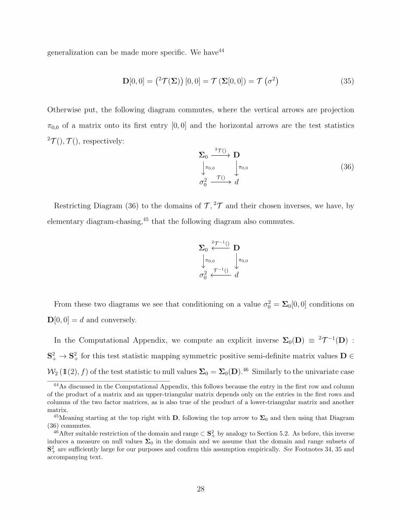
generalization can be made more specific. We have44

D[0, 0] =(

2T (Σ))

[0, 0] = T (Σ[0, 0]) = T(σ2)

(35)

Otherwise put, the following diagram commutes, where the vertical arrows are projection

π0,0 of a matrix onto its first entry [0, 0] and the horizontal arrows are the test statistics

2T (), T (), respectively:

Σ0 D

σ20 d

π0,0

2T ()

π0,0

T ()

(36)

Restricting Diagram (36) to the domains of T , 2T and their chosen inverses, we have, by

elementary diagram-chasing,45 that the following diagram also commutes.

Σ0 D

σ20 d

π0,0 π0,0

2T −1()

T −1()

From these two diagrams we see that conditioning on a value σ20 = Σ0[0, 0] conditions on

D[0, 0] = d and conversely.

In the Computational Appendix, we compute an explicit inverse Σ0(D) ≡ 2T −1(D) :

S2+ → S2

+ for this test statistic mapping symmetric positive semi-definite matrix values D ∈

W2 (11(2), f) of the test statistic to null values Σ0 = Σ0(D).46 Similarly to the univariate case

44As discussed in the Computational Appendix, this follows because the entry in the first row and columnof the product of a matrix and an upper-triangular matrix depends only on the entries in the first rows andcolumns of the two factor matrices, as is also true of the product of a lower-triangular matrix and anothermatrix.

45Meaning starting at the top right with D, following the top arrow to Σ0 and then using that Diagram(36) commutes.

46After suitable restriction of the domain and range ⊂ S2+ by analogy to Section 5.2. As before, this inverse

induces a measure on null values Σ0 in the domain and we assume that the domain and range subsets ofS2

+ are sufficiently large for our purposes and confirm this assumption empirically. See Footnotes 34, 35 andaccompanying text.

28

discussed above, the standardW2 (11(2), f) distribution for the test statistic has distinguished

values and each such value D then corresponds to a particular null value Σ0(D), providing a

conditional sample covariance estimate given the test statistic value D, which we will shorten

to conditional estimate, Σ | D.

A Point Estimate. The mean of the standard WishartW2 (11(2), f) equals f × 11(2), and

therefore choosing Df ≡ f × 11(2) yields the bivariate zero error estimate Σ | Df by analogy

to σ2|f in the univariate case. From Equation (35) above,(Σ | Df

)[0, 0] = (σr)2|f .

Region Estimates. From Equation (34), if RDα 3 Df is a confidence region forW2 (11(2), f)

with significance α, then RΣα ≡ Σ0

(RDα

)= 2T −1

(RDα

)3 Σ0 (Df ) is a confidence region for

Σ | Df with the same significance.47

As shown in the Computational Appendix, the density for a W2 (11(2), f) is a product

of three densities: two χ2f densities corresponding to the two variances of the associated

bivariate Gaussian, and a density ≡ Dρ, up to a normalization factor, of the form p(ρ) =

(1− ρ2)f−32 corresponding to their correlation.48 We may therefore choose for our standard

W2 (11(2), f) confidence region ≡ 0RD

5% a rectangular solid equal to a product of three I1.6%

confidence intervals corresponding to each of (i) the FIR variance, (ii) the stock variance and

(iii) their correlation.49

As we did with the interval estimate for (σr)2, we seek the three-dimensional confidence

region RΣ5% ≡

2T −1(

0RD

5%

). Because de-trending the bivariate series in Equation (32)

requires only a univariate hypothesis (σr0)2, for mechanical ease and efficiency, and simple

2D visualization, we start with our standard (σr)2 confidence interval 0I(σr)2 as before and

47By construction of the pullback measure described in Footnote 34.48In our context the first two of these densities correspond to the FIR and stock variances.49As previously stated, we choose these confidence intervals because there are three parameters to estimate

and (100%− 1.6%)3 = 98.4%3 = 95.3% > 95%. A significance level of 1.6% is thus a conservative cube root

for a significance level of 5%:0RD

5% ≡0I(σr)2 × 0I(σS)

2

× 0Iρ ≈ [0.84, 1.41] × [0.84, 1.41] × [−0.3, 0.3]. Wehave followed the convention that the intervals should be symmetric (after weighting) about their center, 1in the case of χ2

f and 0 in the case of Dρ. See Standard Confidence Interval at the end of Section 5.2.

29

then, conditional on a particular (σr0)2 in this interval, estimate a two-dimensional cross-

sectional confidence region for ρ,(σS)2

: ≡(

Rρ,(σS)

2

3.2% | (σr0)2

)⊂ RΣ

5%. We recover the full

confidence region RΣ5% disjointly from the cross-sections:

RΣ5% =

⋃(σr0)

2∈0I(σr)2

Rρ,(σS)

2

3.2% | (σr0)2 .

Details are left to the Computational Appendix. Conditioned on FIR volatility zero error

estimates (σr)20 ≡ (σr)2|f , Figure (5) shows for ten selected futures pairs the associated

0Rρ,(σS)

2

3.2% , defined as the indicated two-dimensional confidence regions for stock volatility

and stock-FIR correlation at the 3.2% significance level, conditional on the associated zero

error estimate (σr)20 for (σr)2. In Figure (5), each region’s color indicates the associated

level of (σr)20. Figure (6) shows all confidence regions associated with the ninety-five futures

pairs. The Computational Appendix provides details, including similar confidence regions

conditioned on other estimates (σr)2|d ∈0I(σr)2 .

5.5 Estimating the Convexity Adjustment

We restrict the discussion to the confidence regions 0Rρ,(σS)

2

3.2% ≡ Rρ,(σS)

2

3.2% | (σr)20 described

in the prior subsection and leave the general case to the Computational Appendix.

The confidence regions from the prior section are interesting in their own right. In addition,

they imply, via Proposition 4.4, confidence intervals for the FIR convexity adjustment ≡

c(t) = eU1(T2,θ)−U2(t,θ), in which the exponent can be written as a quadratic form defined on

these regions via Equation (22).

Figure (7) contains a graph of the maximum, minimum and average of the convexity

exponent U1(T2, θ)−U2(t, θ) over a 95% confidence interval in each quarterly futures period,

together with a graph of the unadjusted FIR (without any convexity adjustment, based solely

on the IFFR) and contemporaneous market (forward) rates. A quick look at this convexity

30

graph reveals that the average adjustment rarely exceeds a basis point and never exceeds

six basis points. The average convexity adjustment histogram in Figure (8) confirms this

conclusion.

On this basis we conclude that the convexity adjustment is typically negligible at the data

frequencies and time horizons we consider, outside of a small number of periods we will treat

as atypical.

Thus, we take as our estimate of the FIR the unadjusted FIR in the top graph of Figure

(7) and Figure (1).

6 Spread Analysis

Our primary objective in this paper has been to understand the implicit financing cost of

futures investment, which we have addressed above, and its relationship to market rates on

explicit financing, to which we now turn, and which can be expressed through spreads. Our

FIR estimates from the last section permit an estimate of the spreads50 between the FIR

and market rates. To match the FIR terms we take contemporaneous forward Treasury rates

and LIBOR, respectively, as representative of risk-free and financial institution borrowing

rates.51

Figure (9) shows a graph of the estimated FIR-LIBOR and FIR-Treasury spreads with

four regimes superimposed. These regimes are based on a visual review suggesting three

shifts in the behavior of the two spreads over our total observation period: a tightening of

the spreads near the start of 2001, an increase in spread volatility and divergence between

the two spreads midway through 2007, and a reduction in volatility and convergence of the

spreads in 2009.

50The spread equals the FIR minus the indicated contemporaneous market rate. Section [•] of the Compu-tational Appendix describes the methodology we used the determine the forward market rates and associatedFIR spreads. See also the text accompanying Footnote 16 for a general indication of our methodology.

51Id.

31

Motivated by this visual review, we defined the following four separate regimes, generally

determined by reference to the passage of the Commodity Futures Modernization Act of

2000 (“CFMA”) and the 2008 financial crisis:

1. From 1996 until the passage of the CFMA, which we set at the end of 2000.

2. After the CFMA but before the financial crisis, which we treated as beginning in July

of 2007, the month in which “Bear Stearns disclosed that ... two [of its] subprime hedge

funds had lost nearly all of their value amid a rapid decline in the market for subprime

mortgages.”52

3. The financial crisis, which we treated as ending in March 2009, and

4. Recovery from the financial crisis.

The spreads series remained in a range between positive and negative three percent, sug-

gesting mean-reversion. An AR(1) fit (shown in dotted red in Figure (10))) supports mean-

reversion as well.

We therefore treat the spreads series in each regime as Ornstein-Uhlenbeck (OU ) processes,

which we estimate as AR(1) processes,53 viewed as a discrete OU processes, allowing us, for

example, to test hypotheses that the AR(1) reversion mean54 of a spread in a particular

regime was greater, or less, than zero at a specified confidence interval.55

Figure (11) shows the block bootstrapped distribution of the AR(1) means of the two

spread series in each regime and over the entire observation period (last boxplot).56 The col-

ored regions represent block bootstrapped 95% confidence regions for those means, while the

52“Bear Stearns.” Wikipedia: The Free Encyclopedia. Wikimedia Foundation, Inc. September 4, 2016.Web. October 17, 2016.

53First order autoregressive processes.54For an AR(1) of the form xt+1 = c+ bxt + aεt, the reversion mean is defined by µ = c

1−b , equal to thelong-term equilibrium determined by setting εt ≡ 0.

55Equivalently, was the difference between the FIR and the LIBOR or Treasury rate statistically significantin that regime?

56We used a procedure with 10,000 (block) bootstrapped (re)samples and a block length of 20 for eachsubseries. The bootstrap procedure addressed the remaining serial correlation in the AR(1) residuals, butdid not address the possibility that the volatility of the AR(1) residuals varied. Further research couldinclude fitting AR(1) + GARCH(1,1) models to reflect this possibility.

32

Average FIR Spread (bps)

Period LIBOR Rate Treasury Rate

Total (1996 to 2019/6) (6) 38BCI (10)-(1) 34-431996 to 2000 (pre-CFMA) 26 75BCI 18-32 68-812001 to 2007/6 (post-CFMA) (7) 15BCI (15)-2 6-252007/7 to 2009/3 (financial crisis) (73) 56BCI (97)-(37) 29-772009/4 to 2019/6 (recovery) (11) 30BCI (15)-(7) 27-33

Table 1. Forward FIR Spreads to Two Market Rates in Four Regimes with ConfidenceIntervals Based on Block Bootstraps

notches represent those confidence regions determined by conventional bootstraps, showing

the importance of serial correlation to estimation. With the sole exception of the LIBOR

spread in the second regime, each mean is nonzero at the 95% confidence level. The Treasury

spread mean is consistently positive, while the LIBOR spread mean’s sign is positive before

the CFMA but negative thereafter. The associated numeric data appears in Table (1) above,

from which we can see that, excluding the final Treasury spread, the means in consecutive

regimes differ at the 90% significance level.

In this regard, our analysis provides three main findings. First, the mean spreads decreased

after the CFMA’s passage, and this decrease was significant. Second, the mean spreads in

consecutive regimes differed, and this difference was generally significant. Third, over the

entire observation period the mean spread to LIBOR (respectively, the Treasury rate) was

generally negative (resp., consistently positive), but the spread, and in the case of LIBOR

its sign, varied considerably over time and regime.

We can therefore conclude in broad terms that over most of our twenty-four year obser-

vation periods the FIR was above the Treasury rate but below LIBOR, though with many

33

exceptions, some large. Because LIBOR is a market rate associated with unsecured finan-

cial financing, we further conclude in turn that the FIR was generally attractive relative to

unsecured explicit financing available to large financial institutions.

In margin lending, however, the financing is collateralized by purchased securities. The

associated rates vary considerably, but can be close to, or even below, the risk free rate,

particularly if the securities are on ”special”.57

Putting all this together, we conclude that, since the FIR was generally significantly above

the Treasury rate, the evidence from our observation period showed no meaningful systematic

advantage or disadvantage for the FIR relative to the rates on explicit financings, including

margin. On any given date, the FIR could be, and during the observation period was, above

or below the explicit financing rate.

7 Summary

We explored the cost of implicit leverage associated with the S&P 500 equity index futures

contract. We showed that the related implicit financing rate has often been attractive relative

to market rates on explicit financing; however, the relationship between the implicit and

explicit financing rates has been volatile and varied considerably based on legal and economic

regimes. Only rarely was the FIR below the Treasury rate.

These findings depended on accurate estimates of the FIR, which depended in turn on

estimates of the FIR convexity term. We developed new estimation methods for these

purposes with strong similarities to fiducial inference, including point and interval estimates.

57Securities that are hard to borrow are said to be ”on special” and can be lent on favorable terms.Since margin agreements often permit the lender to lend the hypothecated securities, the associated lendingrevenue can reduce the margin rate. Geczy et al. (2002). Each margin lender sets its own margin rate, andhistorical data on a market margin rate level is accordingly difficult to obtain. The broker call money rate isthe rate lenders charge to brokers on loans to finance the brokers’ margin loans to customer. This rate hasbeen observed to be around 1.5 points above the Federal Funds rate. Fortune (2000). From this we see thatmargin lending rates vary considerably and exceed Treasury rates absent unusual circumstances. By way ofcomparison, in our observation period LIBOR exceeded the Treasury rate by 44 basis points on average.

34

In order to estimate the FIR convexity term, we extended our methods to bivariate estimates

of the FIR and equity volatility, Our estimates showed the convexity term could be treated

as insignificant in all but a small number of cases, allowing us to estimate the FIR simply

from the observable futures ratio, adjusted for dividends.

References

Anderson, G. and Kercheval, A. N. (2010). Lectures on Financial Mathematics: Discrete

Asset Pricing. Synthesis Lectures on Mathematics and Statistics. Morgan and Claypool

Publishers.

Anderson, R. M., Bianchi, S. W., and Goldberg, L. R. (2012). Will my risk parity strategy

outperform? Financial Analysts Journal, 68(6):75–93.

Anderson, R. M., Bianchi, S. W., and Goldberg, L. R. (2014). Determinants of levered

portfolio performance Financial Analysts Journal, 70(5):53–72.

Anderson, R. M., Eom, K. S., Hahn, S. B. and Park, J. H. (2013). Autocorrelation and

partial price adjustment Journal of Empirical Finance, 24:78–93.

Bali, T. G. and Demirtas,K. 0. (2008) Testing Mean Reversion In Financial Market Volatility:

Evidence From S&P 500 Index Futures The Journal of Futures Markets, 28(1): 1–33

Black, F. (1976) The Pricing of Commodity Contracts Journal of Financial Economics, 3:

167-175

Breeden, D. T. and Litzenberger, R. H. (1978) Prices of State-contingent Claims Implicit in

Option Prices Journal of Business, 51(4): 621–51

Chan, K., Chan, K. C. and Karolyi,G. A. (1991) Intraday Volatility in the Stock Index and

Stock Index Futures Markets The Review of Financial Studies, 4(4): 657-684

35

Chen, W. P., Chung, H. and Lien, D. (2016) Price discovery in the S&P 500 index derivatives

markets, International Review of Economics and Finance, 45: 438–452

Cox, J., Ingersoll, J. and Ross,S. (1981) The Relation Between Forward Prices and Futures

Prices Journal of Financial Economics, 9: 321-347

Dwyer, G., Locke, P. and Yu, W. (1996). Index Arbitrage and Nonlinear Dynamics Between

the S&P 500 Futures and Cash The Review of Financial Studies, 9(1):301-332

Fisher, R. A. (1935). The Fiducial Argument In Statistical Inference Annals of Eugenics,

6:391-98

Fortune, P. (2000). Margin Requirements, Margin Loans, and Margin Rates: Principles and

Practice New England Economic Review, 20 (September/October):31

Geczy, C. et al., (2002). Stocks are Special Too: An Analysis of the Equity Lending Market

Journal of Financial Economics, 66, 241-269, (10.1016/S0304-405X(02)00225-8)

Hilliard, J. E., Hilliard, J. and Ni, Y. (2021). Using the short-lived arbitrage model to

compute minimum variance hedge ratios: application to indices, stocks and commodities

Quantitative Finance 21:1, 125-142, available at:https://www.tandfonline.com/loi/rquf20

Jegadeesh, N. and Pennacch, b. (1996). The Behavior of Interest Rates Implied by the Term

Structure of Eurodollar Futures Journal of Money, Credit, and Banking 28(3/2):426-46

Kenourgios, K. Samitas, A. and Droso, P. (2000). Hedge ratio estimation and hedging

effectiveness: the case of the S&P 500 stock index futures contract International Journal

of Risk Assessment and Management 9(1/2):121-34

Lien, D. (2004). Cointegration and the optimal hedge ratio: the general case The Quarterly

Review of Economics and Finance 44: 654–658

Otto, M. (2000) Stochastic relaxational dynamics applied to finance: Towards non-

equilibrium option pricing theory. Eur. Phys. J. B. 14:383–394

36

Poon, S. and Granger, C. (2003) Forecasting Volatility in Financial Markets: A Review

Journal of Economic Literature 41(2): 478-539.

37

Fig

ure

1.

Unad

just

edF

IRE

stim

ates

vs

Mar

ket

Rat

es

38

Fig

ure

2.

(σr)2|f

vs

ML

EE

stim

ates

39

Fig

ure

3.θ|f

vs

ML

EE

stim

ates

40

Fig

ure

4.

(σr)2|f

Est

imat

esw

ith

98.4

%C

onfiden

ceIn

terv

als

41

Fig

ure

5.

Sel

ect

Con

fiden

ceR

egio

ns

42

Fig

ure

6.

All

Con

fiden

ceR

egio

ns

43

Fig

ure

7.

Unad

just

edF

IR,

Mar

ket

Rat

esan

dC

onve

xit

yA

dju

stm

ent

95%

CIs

44

Fig

ure

8.

His

togr

amof

Ave

rage

Con

vexit

yA

dju

stm

ent

over

95%

CIs

45

Fig

ure

9.

FIR

Spre

adM

ean

Rev

ersi

onin

Fou

rR

egim

es

46

Fig

ure

10.

FIR

Spre

adA

R(1

)F

its

47

Fig

ure

11.

FIR

Spre

adA

R(1

)M

eans

48