The impacts of duct design on life cycle costs of central...

Accepted Manuscript

Title: The impacts of duct design on life cycle costs of centralresidential heating and air-conditioning systems

Author: Brent Stephens

PII: S0378-7788(14)00594-5DOI: http://dx.doi.org/doi:10.1016/j.enbuild.2014.07.054Reference: ENB 5206

To appear in: ENB

Received date: 18-4-2014Accepted date: 24-7-2014

Please cite this article as: B. Stephens, The impacts of duct design on life cycle costs ofcentral residential heating and air-conditioning systems, Energy and Buildings (2014),http://dx.doi.org/10.1016/j.enbuild.2014.07.054

This is a PDF file of an unedited manuscript that has been accepted for publication.As a service to our customers we are providing this early version of the manuscript.The manuscript will undergo copyediting, typesetting, and review of the resulting proofbefore it is published in its final form. Please note that during the production processerrors may be discovered which could affect the content, and all legal disclaimers thatapply to the journal pertain.

http://dx.doi.org/doi:10.1016/j.enbuild.2014.07.054

http://dx.doi.org/10.1016/j.enbuild.2014.07.054

of 46

Accep

ted M

anus

cript

1

The impacts of duct design on life cycle costs of central residential heating and air-conditioning systems Brent Stephens, PhD1,* 1Department of Civil, Architectural and Environmental Engineering, Illinois Institute of Technology, Chicago, IL USA *Corresponding author: Brent Stephens, Ph.D. Assistant Professor Department of Civil, Architectural and Environmental Engineering Illinois Institute of Technology Alumni Memorial Hall Room 212 3201 South Dearborn Street Chicago, IL 60616 Phone: (312) 567-3356 Email: [email protected]

of 46

Accep

ted M

anus

cript

2

The impacts of duct design on life cycle costs of central residential heating and air-conditioning systems Brent Stephens, PhD1,* 1Department of Civil, Architectural and Environmental Engineering, Illinois Institute of Technology, Chicago, IL USA *Corresponding author: [email protected]

Abstract

Many central residential HVAC systems in the U.S. operate at high external static

pressures due to a combination of system restrictions. Undersized and constricted ductwork are

thought to be key culprits that lead to excess external static pressures in many systems, although

the magnitude of energy impacts associated with restrictive ductwork and the costs or benefits

associated with addressing the problem are not well known. Therefore, this work uses annual

energy simulations of two new single-family homes in two separate climates in the United States

(Austin, TX and Chicago, IL) to predict the impacts of low, medium, and high external static

pressure ductwork designs from independent HVAC contractors (using both flexible and rigid

sheet metal ductwork materials) on annual space conditioning energy use. Results from the

simulations are combined with estimates of the initial installation costs of each duct design made

by each contractor to evaluate the total life cycle costs or savings of using lower pressure duct

designs in the two homes over a 15-year life cycle. Lower pressure ductwork systems generally

yielded life cycle cost savings, particularly in homes with PSC blowers and particularly when

making comparisons with constant ductwork materials (i.e., comparing flex only or rigid only).

Keywords: HVAC, EnergyPlus, BEopt, energy simulation, air-conditioning, static pressures

of 46

Accep

ted M

anus

cript

3

1. Introduction

Many central residential heating, ventilating, and air-conditioning (HVAC) systems in the

U.S. have substantially higher external static pressures than specified by most standardized test

procedures [1] due to a combination of common system restrictions, including high pressure drop

filters, cooling coils, heating elements, ductwork, and fittings [2–8]. Among these restrictions,

undersized and constricted ductwork is thought to be a key culprit that leads to excess external

static pressures that a system must overcome, particularly for compressible flexible ductwork

materials [9]. Excess static pressures can have negative energy impacts depending on the type of

blower motor used in the air handling unit (AHU) and the level of excess static pressure [10,11].

Increasing diameters in duct designs and specifying low-resistance duct materials can reduce

system pressures [12] but may also increase the surface area for heat transfer to occur across

ductwork installed in unconditioned spaces [13]. Consequently, the combined impacts of duct

design details and external static pressures on energy consumption are complex, as the

relationships between pressure, fan efficiency, fan power draw, airflow rates, and heating and

cooling capacities are not straightforward and depend on the type of blower motor used in the

AHU. Additionally, there is a lack of information on the overall life cycle cost implications of

lower static pressure duct designs for central residential HVAC systems. Therefore, this work

summarizes the potential impacts of high pressure duct designs on factors influencing central

residential HVAC energy consumption and uses a combination of energy modeling and life cycle

cost analysis to simulate the net life cycle impacts of lower pressure duct designs in residences.

2. Background

The energy impacts of varied external static pressures can be categorized generally into

(1) direct power draw requirements of the AHU fan, and (2) more complex and indirect

of 46

Accep

ted M

anus

cript

4

relationships between pressure, airflow, delivered sensible and latent capacities, system runtimes,

and heat transfer across ductwork surfaces (if ductwork is installed in unconditioned spaces). For

direct energy impacts, the fan power draw requirements of any AHU blower are determined by

system pressure, airflow rates, and fan and motor efficiencies as shown in Equation 1.

(1)

where Wfan = power draw of the fan (W); ǻPsystem = external system pressure (Pa); Qfan = airflow

rate (m3 s-1); Șfan = efficiency of the fan (-); and Șmotor = the efficiency of the fan motor (-).

Depending on the type of blower motor used, the airflow rate (Qfan) and the overall efficiency

(Șfan×Șmotor) will respond differently to a specific external static pressure (ǻPsystem) and thus will

have different impacts on fan power draw.

Permanent split capacitor (PSC) motors have traditionally been the most widely used

technology in residential AHU blowers in the U.S. with a market share of approximately 90% as

of 2002 [14], although the share has decreased some in recent years. PSC blowers do not

incorporate controls to maintain airflow rates at constant rates. Therefore, when excess system

pressures are introduced, airflow rates typically decrease [7,8,11]. For most parts along the fan

curve, increasing the external static pressure and decreasing airflow rates will reduce the power

draw of a PSC blower, although the direction and magnitude of changes in fan power draw also

depend on the location along the fan efficiency curve [7].

The overall energy impacts of reduced airflows are more complex. Reducing system

airflow rates in systems with PSC blowers will decrease the cooling capacity of vapor

compression air-conditioning systems, although changes in sensible and latent capacity are

typically nonlinear with flow reductions [11,15]. Decreased sensible capacity will lead to

increased energy consumption for space conditioning by increasing the length of system runtime,

of 46

Accep

ted M

anus

cript

5

although very few measurements of these impacts have been made in actual homes. Capturing

these effects is important; because the power draw of outdoor compressor-condenser units is

typically much larger than the power draw of AHU fans [7,8], even a small increase in system

runtime may overwhelm any savings in fan power draw. Complicating things further, reduced

airflow rates have also been shown to reduce compressor power draw [11,15], which may offset

some of the energy impacts of increased runtimes, depending on the magnitude of each change.

For heat pumps, lower airflow rates will generally decrease both heating and cooling capacity as

well, although the power draw of outdoor units will typically increase [16].

Electronically commutated motors (ECMs), also known as brushless permanent magnet

motors (BPMs), utilize variable speed motors and drives that are designed to maintain constant

or near-constant airflow rates across a wide range of external static pressures [17]. ECM blowers

typically also have a much higher electric conversion efficiency than PSC blowers across a wider

range of airflow rates [3,18–20]. In these systems, an increase in system pressure will generally

result in an increase in fan power draw and thus fan energy consumption in order to maintain the

same (or nearly the same) airflow rate [21], depending on the sophistication of control systems

utilized [22]. The absolute magnitude of power draw will still usually be lower than a PSC motor

because of typically higher efficiencies at most airflow rates, depending on the magnitude of the

pressure increase. Because ECM blowers adjust to maintain airflow rates, altering duct system

pressures will not drastically impact indirect energy consumption by altering system runtimes;

energy impacts are primarily derived from direct fan power impacts. However, overall space

conditioning energy impacts can still be more complex and may vary by climate. For example, at

higher fan power draws at higher pressures, more excess heat will be rejected into the airstream,

of 46

Accep

ted M

anus

cript

6

which may increase cooling energy requirements but may also decrease heating energy

requirements [23].

Given the complexity of these relationships between external static pressure, airflow

rates, fan power draws, fan efficiencies, sensible and latent capacities, system runtimes, and the

combined impacts on space conditioning energy consumption, we have conducted a modeling

effort to explore the overall impacts on energy consumption and life cycle costs of various duct

designs in two typical single-family homes in both hot and cold U.S. climates: Chicago, IL, and

Austin, TX. Three external static pressures (ǻPsystem) were initially specified as design targets

(low, medium, and high) in each home and independent HVAC contractors provided ductwork

designs and cost estimates for each duct system in each home as if they were to actually perform

the design and installation. Details of the duct designs and system configurations (including two

types of ductwork materials, rigid and flex) at the various external pressures were combined with

typical fan and system curves for equipment to provide inputs for whole building energy analysis

in order to explore these complex relationships in the two model homes.

3. Methodology

The following sections describe the selection of model homes; determinations of inputs

for target system pressures, airflow rates, and fan power draws; estimation of duct UA values

from the contractors’ designs; the energy simulation procedures; and methods for conducting life

cycle cost analyses. More details are described in the full project report [24].

3.1 Model home selection

House plans for (i) a typical one-story single-family home with an unconditioned

basement in the Midwestern U.S. (Chicago, IL) and (ii) a typical one-story slab-on-grade single-

family home in the Southern U.S. (Austin, TX) were first identified by an independent

of 46

Accep

ted M

anus

cript

7

residential HVAC contractor in each location. The homes were designed to meet or exceed most

minimum energy code requirements in both locations according to the 2009 International Energy

Conservation Code (IECC). Relevant building characteristics are described in detail in Table 1.

These homes are considered to be generally consistent with new residential construction

practices in each location.

Table 1. Baseline characteristics of each IECC 2009 compliant home in each location Austin, TX Chicago, IL Floor area (m2) 293 195 Orientation Front door faces southeast Front door faces east

Floor construction Slab on grade Full unconditioned basement R-SI 5.28 floor insulation

Number of bedrooms 3 3 Number of bathrooms 2 2 Exterior materials Stucco and stone exterior Brick veneer Wall insulation (m²·K/W) R-SI 3.35 in 5x15 cm studs R-SI 3.70 in 5x15 cm studs Attic insulation (m²·K/W) R-SI 6.69 in roof deck R-SI 6.69 in roof deck Window U-value (W/m²·K) 2.0 2.0 Window SHGC 0.30 0.55 Window area, F B L R (m2) 8.3, 18.6, 11.1, 3.3 4.5, 10.4, 0.8, 1.1 Duct/AHU location Unconditioned attic Unfinished basement Duct insulation (m²·K/W) R-SI 1.06 R-SI 1.06 Duct leakage (%) 10% 10% Envelope airtightness 7 ACH50 7 ACH50

Modeled HVAC equipment 1-stage heat pump

4.76 rated COP cooling 3.91 rated COP heating

1-stage DX AC unit 4.76 rated COP cooling

92.5% AFUE gas furnace Nominal AHU airflow rate (m3 hr-1) 2040 @ 125 Pa 2720 @ 125 Pa Nominal cooling capacity (kW)* 14.1 kW (SHR = 0.74) 10.6 kW (SHR = 0.74) Nominal heating capacity (kW)* 14.1 kW (+ 2.93 kW suppl.) 19.9 kW *Model system capacities reflect values modeled at the nominal (highest) airflow rate assumed for each home.

3.2 Pressure, airflow, and fan power determinations

The smaller Chicago home was chosen to have a nominal airflow rate of 2040 m3 hr-1

with ducts installed in the unconditioned basement and the larger Austin home had a nominal

airflow rate of 2720 m3 hr-1 with ducts installed in the unconditioned attic. We then specified a

range of three target external static pressures (ǻPsystem) to explore based on the size of each

system, defined as “low,” “medium,” and “high” static pressures herein. These pressures were

chosen to accurately reflect a wide, albeit realistic, range observed in real homes in the field and

of 46

Accep

ted M

anus

cript

8

to represent the total pressure introduced by a combination of ductwork, coils, filters, supply

registers, and return grilles. Table 2 summarizes the total external static pressures associated with

each targeted design: 125 Pa, 200 Pa, and 275 Pa were used as the low, medium, and high

pressures in the Chicago home and 138 Pa, 213 Pa, and 288 Pa were used in the larger Austin

home. Table 2 also shows the external static pressures introduced by ducts alone after assuming

87 Pa is introduced by the combination of filters (25 Pa), coils (40 Pa), registers (8 Pa), and

grilles (8 Pa). These assumptions are widely used in ACCA Manual D calculations [25].

Although the system pressures identified in Table 2 are higher than standard industry

assumptions and test conditions [1], they actually compare very well with existing measurements

of pressures in real homes across the U.S. For example, in a study of 60 new homes in

California, total external pressures during cooling periods ranged from ~75 Pa to ~300 Pa [26].

Similarly high static pressures were also measured in other recent field studies [6–8,27,28]. Thus

our target design pressures for low, medium, and high static pressure duct designs are considered

realistic across the U.S. residential building stock.

The specified pressures and home plans were then used by each of the independent

HVAC contractors in performing ACCA Manual D calculations to size and specify different

ductwork designs to achieve each external pressure in each home [25]. Each contractor provided

their designs along with a cost estimate for the design and installation of each duct system in

each homes as if they were to actually perform the installation. Duct designs were also made for

each target pressure using two different duct materials: (1) flex ductwork and (2) rigid sheet

metal ductwork. Both contractors performed duct designs and cost estimates for each home;

therefore, their results capture regional variations in material selections, labor costs, and

construction practices for both homes. Each contractor provided a total of 12 duct designs and

of 46

Accep

ted M

anus

cript

9

cost estimates covering the two homes, each with three pressures and two duct materials. These

designs captured real life variability in duct diameters, layouts, lengths, and materials that real

contractors would use to achieve the target low, medium, or high external static pressures.

The low, medium, and high external static pressures were then used to estimate the

impacts of system pressures on fan airflow rates, fan efficiencies, and fan power draws in each

home, treating PSC and ECM blowers separately, which were then used as inputs to annual

building energy simulations in EnergyPlus [29]. Data were selected for these inputs to be as

widely representative of residential HVAC equipment as possible by relying on “virtual models”

from a large summary of manufacturer fan data provided in Appendix 7-F of the Technical

Support Document for the Energy Efficiency Program for Consumer Products: Residential

Central Air Conditioners, Heat Pumps, and Furnaces [21].

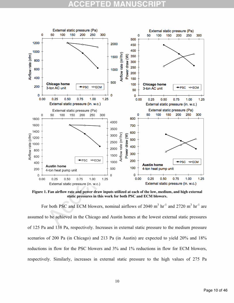
Representative fan curves (airflow vs. pressure) and fan power curves (power vs.

pressure) for a range of single-stage virtual model furnaces with both PSC and ECM blowers are

shown in Figure 1. The target low, medium, and high static pressures are marked on each graph

for both homes. These virtual models show that excess static pressures decrease airflow rates

with PSC blowers and that fan efficiency (in units of W cfm-1) remains largely constant until

pressures in excess of ~190 Pa, meaning that fan power draw will generally decrease with

decreases in fan flow. Conversely, the representative ECM blowers respond to excess pressure

by maintaining near-constant flows, with fan power draw increasing almost linearly with airflow.

Curve fits to the data in the technical support document were used to extend the range of external

pressures beyond the scale shown in the original figures.

of 46

Accep

ted M

anus

cript

10

Figure 1. Fan airflow rate and power draw inputs utilized at each of the low, medium, and high external static pressures in this work for both PSC and ECM blowers.

For both PSC and ECM blowers, nominal airflows of 2040 m3 hr-1 and 2720 m3 hr-1 are

assumed to be achieved in the Chicago and Austin homes at the lowest external static pressures

of 125 Pa and 138 Pa, respectively. Increases in external static pressure to the medium pressure

scenarios of 200 Pa (in Chicago) and 213 Pa (in Austin) are expected to yield 20% and 18%

reductions in flow for the PSC blowers and 3% and 1% reductions in flow for ECM blowers,

respectively. Similarly, increases in external static pressure to the high values of 275 Pa

of 46

Accep

ted M

anus

cript

11

(Chicago) and 288 Pa (Austin) yield 48% and 43% reductions in flow for PSC blowers and 8%

and 2% reductions in flow for ECM blowers, relative to the low pressure cases.

For the Chicago home, these flow changes correspond to as much as a 41% reduction in

fan power draw (PSC) and as much as a 42% increase in fan power draw (ECM) at the highest

pressure relative to the lowest pressure. At the highest pressure the PSC blower will actually

draw less power than the ECM blower. Similarly for the Austin home, the highest pressure yields

a 36% decrease in fan power draw by the PSC blower and a 55% increase in fan power draw by

the ECM blower relative to the lowest pressure scenario; power draw is approximately equal for

both blowers at the highest pressure. These pressure, flow, and power draw changes are

generally consistent not only with manufacturer data but with data from other laboratory and

field tests [7,8,11,20,27], and thus should be considered generally representative of the range of

equipment and operational conditions observed in homes across the country. The absolute values

of the full range of pressure, airflow, fan power draw, and fan efficiency inputs for each

simulation case in both homes are shown in Table 2. Once airflow and fan power draw impacts

in response to the defined target static pressures were identified, those data were then used as

inputs to EnergyPlus, which utilized built-in polynomial functions that calculate heating and

cooling capacity, COP (which is the inverse of the energy input ratio, EIR), and outdoor unit

power draw as a function airflow rates using generic air-conditioning, heat pump, and furnace

models.

3.3 Duct UA values

Duct surface areas and duct UA values were also estimated for each modeled scenario

based on the contractor duct designs to capture indirect energy impacts of heat transfer across

ducts installed in unconditioned spaces [13,30,31]. Although duct insulation values were

of 46

Accep

ted M

anus

cript

12

constant in both homes and in all scenarios (R-SI 1.06 m²·K/W), the surface areas of supply and

return ductwork varied according to each duct design, which affects the overall UA values for

ductwork. Supply and return ductwork surface areas of each ductwork design were estimated

manually based on the size and shape of ductwork provided by the contractors (i.e., by

calculating the surface area of a cylinder of the same length and diameter as each duct run).

Those values were converted into UA values for each scenario based on ductwork with U = 0.94

W/m²·K.

The ductwork designs for lower external static pressures from the contractors generally

utilized greater diameter ductwork that was typically running similar lengths (the greater

diameter allows for lower resistance for an equivalent length). Therefore, the external surface

area of ductwork was typically higher for the lower static pressure designs, although there was

considerable variability between the two contractors’ designs. Designs by the Chicago contractor

resulted in UA values for ductwork that were typically 20-30% higher for the lower pressure

(larger diameter) duct systems relative to the highest pressure (smaller diameter) duct systems;

designs by the Austin contractor resulted in UA values that were between 2% and 15% higher for

the lower pressure systems. Additionally, the Austin contractor tended to use more efficient duct

designs in terms of material; their duct UA values were often 20-40% lower than the Chicago

contractors. For example, the Austin contractor relied on flexible duct trunks and branches to

achieve the desired pressure for each scenario while the Chicago contractor utilized a radial flex

duct design where each branch began at the AHU (this is often referred to “ductopus”

configuration as the branches resemble the tentacles of a cephalopod).

of 46

Accep

ted M

anus

cript

13

Table 2. Summary of pressure, flow, fan efficiency, fan power, and duct UA inputs for the EnergyPlus simulations

Duct UA (W/K) Chicago

contractor Austin

contractor Home Duct type

Blower type

Duct pressure

(Pa)

Total pressure

(Pa)

Airflow rate

(m3 hr-1)

Fan efficiency

(%)

Fan power draw (W) Supply Return Supply Return

38 125 2040 0.16 449 119 59 87 0.7 113 200 1638 0.25 369 90 48 70 0.3 PSC 188 275 1056 0.30 265 85 44 76 0.3 38 125 2040 0.27 260 119 59 87 0.7

113 200 1975 0.33 330 90 48 70 0.3

Flex

ECM 188 275 1875 0.39 369 85 44 76 0.3 38 125 2040 0.16 449 74 35 61 0.3

113 200 1638 0.25 369 58 27 60 0.3 PSC 188 275 1056 0.30 265 57 27 60 0.3 38 125 2040 0.27 260 74 35 61 0.3

113 200 1975 0.33 330 58 27 60 0.3

Chicago home

Ducts in basement

2040 m3 hr-1

airflow nominal

10.6 kW AC

unit

19.9 kW Gas furnace

Rigid Metal

ECM 188 275 1875 0.39 369 57 27 60 0.3 50 138 2720 0.18 573 171 58 105 22

125 213 2236 0.27 482 139 57 100 20 PSC 200 288 1557 0.34 369 137 57 97 20 50 138 2720 0.32 329 171 58 105 22

125 213 2701 0.37 427 139 57 100 20

Flex

ECM 200 288 2660 0.42 510 137 57 97 20 50 138 2720 0.18 573 83 49 108 0.9

125 213 2236 0.27 482 71 45 98 0.9 PSC 200 288 1557 0.34 369 66 44 97 0.9 50 138 2720 0.32 329 83 49 108 0.9

125 213 2701 0.37 427 71 45 98 0.9

Austin home

Ducts in attic

2720 m3 hr-1 airflow nominal

14.1 kW heat

pump Rigid Metal

ECM 200 288 2660 0.42 510 66 44 97 0.9

3.4 Energy simulation procedures

A total of 48 annual energy simulations were performed in EnergyPlus Version 8.1.0

using the appropriate (Chicago and Austin) typical meteorological year (TMY3) data and all of

the combinations of input scenarios covering the two contractors’ duct designs and UA values,

three levels of external static pressure, two types of AHU blowers, and the two homes in the two

climates. BEopt Version 2.1.0.0 was first used to generate EnergyPlus input files (IDF files) for

of 46

Accep

ted M

anus

cript

14

each of the two homes based on geometry and the basic inputs from Table 1. All inputs related to

occupant activity, such as natural ventilation (i.e., window opening) during mild weather and

appliance, lighting, and miscellaneous load profiles, were chosen as the default values in BEopt,

which relies on the well-established inputs in the Building America House Simulation Protocols.

Once all available inputs were selected in BEopt, a single simulation for each home was

run in order to generate an EnergyPlus input (IDF) file. The IDF file was copied for each home

and the results of the initial simulation were discarded because not all inputs were accurate at this

stage. The IDF file was then directly edited using a simple text editor to vary input parameters to

reflect each simulation case. Rated airflow rates for HVAC equipment and duct sizes were kept

at the maximum (nominal, or lowest pressure) value for each simulation case, but the design and

specified airflow rates were adjusted in each case (and capacities and EIR were adjusted

automatically within EnergyPlus using built-in algorithms). Airflow rates were changed in each

of the following sections of the IDF files: AirLoopHVAC:UnitaryHeatCool, Fan:OnOff,

AirTerminal:SingleDuct:Uncontrolled, and Branch. Fan pressure and efficiency were

also changed for each case (in the Fan:OnOff section of the IDF file), which governs fan power

draw in the simulations. Finally, duct UA values were adjusted for each case in a separate section

of the IDF file that is created by BEopt (EnergyManagementSystem:Program).

The homes were modeled without a dedicated outdoor air supply or heat recovery system.

Thermostat set points were 24.4°C in the summer and 21.1°C in the winter. The same airflow

rates were assumed for both heating and cooling modes for simplicity. Important EnergyPlus

outputs for the Chicago home included annual electric use for the AHU fan and outdoor

condenser-compressor unit, as well as annual natural gas usage for the furnace. Similar annual

outputs for the Austin home included electric use for the AHU fan and heat pump during both

of 46

Accep

ted M

anus

cript

15

heating and cooling modes. In this work, “cooling energy” refers to the energy used by the

compressor unit; “heating energy” refers to energy used by either the furnace or the heat pump

unit during heating mode; “fan energy” refers to the total amount of energy used by the AHU fan

during both heating and cooling modes; and total “HVAC energy” refers to the combination of

fan, compressor, and furnace energy use. These annual outputs were first used to explore impacts

of blower types and duct designs on total HVAC energy use and costs on an annual basis using

baseline energy cost estimates. The same results were also used to explore life cycle costs, using

methods described below.

3.5 Life cycle cost estimation

Estimates of annual HVAC energy consumption and costs were summed over an

assumed 15-year lifetime of the HVAC equipment to determine the estimated total lifetime

HVAC energy consumption of each configuration. A 15-year lifetime was chosen as the life

cycle length because although ductwork materials should last much longer, the actual systems

modeled herein (and all of their associated capacity and efficiency inputs) are likely to be

replaced within 15 years. However, a 30-year lifespan was also later considered to explore

sensitivity to this assumption, although it still does not include equipment replacement costs

because the efficiency and capital costs of equipment available 15 years from now are unknown.

National average residential electricity rates and natural gas costs were used in both homes.

Natural gas costs were assumed to remain constant at the 10-year residential average of $11 USD

per GJ, primarily because of recent decreases in gas costs that disrupt any clear trend in costs and

because of historical difficulty in accurately forecasting natural gas prices [32]. Nominal

electricity costs were assumed to be $0.118 USD per kWh in the present year [33], increasing at

a nominal rate of 2.0% per year, or 0.3% in real (2011) dollars [34].

of 46

Accep

ted M

anus

cript

16

To explore the upfront costs and life cycle operational costs or benefits of each duct

design scenario, we first compared differences in upfront costs between each duct design to

differences in cumulative energy costs summed over 15 years of life, accounting for both

increases in energy costs and inflation. This allowed for a comparison between the excess costs

of a design to any added benefit (in terms of operational energy cost savings) or added cost (in

terms of additional operational energy costs required) over the assumed lifespan of 15 years. The

highest pressure (i.e., 275 Pa or 288 Pa) ductwork design was first used as the reference case for

other scenarios to compare to, treating rigid and flex ductwork materials separately. The analysis

was performed separately for PSC and ECM fans because we have not attempted to capture

differences in initial costs for these fan types. An additional comparison was also made across

both flex and metal ductwork to capture the costs and benefits of using different pressure

ductwork designs with different materials, although this analysis is somewhat limited as

described in a later section.

The results from the cost-benefit analysis above were also converted into a net present

value (NPV) as another way to compare life cycle costs and benefits associated with investment

in the various ductwork designs. The annual NPV was estimated for each scenario according to

Equation 2, which follows a procedure outlined in the 2012 Supplement to NIST Handbook 135

Life-Cycle Costing Manual for the Federal Energy Management Program [35].

(2)

where ǻCn = the difference in annual energy cost for space conditioning between a particular

duct design configuration and the baseline configuration in year n; d = the discount rate

(assumed 3.5% based on a 3.0% real rate excluding inflation and a 0.5% long-term average

of 46

Accep

ted M

anus

cript

17

inflation rate, as described in Rushing et al. [35]); and n = the year of analysis. The total NPV

over the course of a 15-year life cycle was then estimated according to Equation 3.

(3)

where NPVlifecycle is the sum of the NPVn for each of the 15 assumed years of the design life

cycle, including the cost of implementation of ductwork in year 0. This yields the total NPV,

which can be used to evaluate whether or not an investment will be beneficial or costly over its

lifetime compared to a reference scenario. In this work, a positive life cycle NPV describes an

investment in which life cycle benefits exceed costs relative to the highest pressure reference

scenarios (i.e., positive NPV = savings). Conversely, a negative NPV describes an investment in

which costs exceed benefits over the duration of the design life cycle (i.e., negative NPV =

excess costs).

4. Results

4.1 Initial costs of duct designs

Table 3 shows the initial design and installation cost estimates for each duct design and

installation in each home from both HVAC contractors. These estimates provide the starting

point for differences in installation costs to which differences in annual energy savings (or excess

costs) are compared for each configuration. For both the Austin and Chicago home duct designs

by the Chicago contractor, lower pressure ducts were consistently more expensive than higher

pressure duct designs. For example, the lowest pressure flex duct would cost approximately $150

USD more than the highest pressure flex duct (~3% higher) in the Chicago home; the same

comparison yields an excess cost of $1250 in the Austin home (~26% higher costs). Similarly,

the lowest pressure sheet metal duct was estimated to cost $1650 more than the highest pressure

of 46

Accep

ted M

anus

cript

18

metal duct (~19% higher) in the Chicago home and $900 more (~8% higher) in the Austin home.

These differences are attributed to both differences in ductwork material (between flex and rigid)

and labor to perform the installations.

For both the Austin and Chicago home duct designs by the Austin contractor, differences

between lower pressure and higher pressure duct costs were not as straightforward. For example,

the lowest pressure flex duct would cost approximately $119 less than the highest pressure flex

duct in the Chicago home; the same comparison yields an excess cost of only $68 in the Austin

home. The medium pressure duct design even had the highest cost in one set of designs.

Similarly, the lowest pressure sheet metal duct was estimated to cost only $9 more than the

highest pressure metal duct in the Chicago home and only $192 more in the Austin home. These

differences are attributed to a combination of differences in ductwork material (between flex and

rigid), the design diameters of ductwork runs, and the labor requirements for installation.

Obviously the two contractors delivered very different designs and cost estimates to meet

the same goals, which is important to capture in the analysis herein. Overall, duct design and

installation is estimated to cost less for the smaller Chicago home according to both contractors,

which is intuitive for the smaller amount of materials involved. Also, for both contractors, rigid

sheet metal ductwork is estimated to cost substantially more than flex duct for all scenarios, as

much as $6000 more for some equivalent configurations. This large excess initial cost is due not

only to differences in materials but in estimates of the more intensive level of labor required to

install rigid ductwork relative to flexible ductwork. Finally, it is important to note that the design

and installation estimates from the Austin contractor were consistently lower for all

configurations, primarily reflecting differences in labor and material costs between Austin, TX

and Chicago, IL.

of 46

Accep

ted M

anus

cript

19

Table 3. Duct design and installation cost estimates from the hired contractors Initial design and installation cost

Chicago contractor Austin contractor Duct material Duct pressure (Pa)

Total external static pressure (Pa) Chicago home

38 125 $4,970 $3,784 113 200 $4,870 $3,665 Flex duct 188 275 $4,820 $3,903 38 125 $10,470 $7,370

113 200 $8,970 $7,423 Rigid sheet metal 188 275 $8,820 $7,361

Austin home 50 138 $6,110 $4,182

125 213 $5,360 $4,160 Flex duct 200 288 $4,860 $4,114 50 138 $11,410 $7,324

125 213 $10,910 $7,160 Rigid sheet metal 200 288 $10,510 $7,132

4.2 Annual energy simulation results

A full table of results from all 48 simulations for both homes with duct designs from both

contractors is shown in Table 4. Results are limited to annual energy use for space conditioning

(i.e., “HVAC energy”), including heating, cooling, and fan energy in each case. Other non-

HVAC energy consumption is excluded from these results because they are unaffected by the

input variables used herein, although it should be noted that heating energy accounted for ~68-

73% of the total amount of predicted natural gas usage in the Chicago home, on average, while

fan and cooling energy accounted for only ~8% and ~6% of total electricity usage, respectively,

across all scenarios and duct designs by both contractors. Space conditioning energy use

accounted for only 36-47% of the total amount of predicted electricity usage in the Austin home,

depending on configuration.

of 46

Accep

ted M

anus

cript

20

Table 4. Annual energy simulation results for both homes using both contractors’ designs

Chicago contractor Austin contractor

Home Duct type

Blower type

Total pressure

(Pa)

Airflow rate

(m3 hr-1)

Coolingenergy (kWh)

Fan energy(kWh)

Heating energy (GJ)

Cooling energy (kWh)

Fan energy (kWh)

Heating energy (GJ)

125 2040 631 556 66.45 619 542 64.31 200 1638 672 539 66.06 661 531 64.28 PSC 275 1056 792 603 68.49 786 600 67.22 125 2040 622 328 67.10 611 319 64.94 200 1975 622 417 65.34 614 411 63.80

Flex

ECM 275 1875 633 481 65.11 631 478 64.21 125 2040 614 536 63.84 611 531 62.80 200 1638 656 522 63.70 656 525 63.57 PSC 275 1056 767 578 65.62 769 583 65.59 125 2040 606 317 64.46 603 314 63.41 200 1975 608 406 63.31 611 406 63.19

Chicago home

Ducts in basement


10.6 kW AC unit

19.9 kW

Gas furnace Metal

ECM 275 1875 622 469 63.26 625 472 63.20

Chicago contractor Austin contractor

Total pressure

(Pa)

Airflow rate

(m3 hr-1)

Coolingenergy (kWh)

Fan energy(kWh)

Heatingenergy (kWh)

Cooling energy (kWh)

Fan energy (kWh)

Heating energy (kWh)

138 2720 2797 964 2261 2342 808 1822 213 2236 2789 817 2369 2461 722 2042 PSC 288 1557 3183 719 3244 2753 622 2722 138 2720 2747 539 2311 2303 453 1856 213 2701 2578 672 2100 2294 597 1819

Flex

ECM 288 2660 2594 789 2094 2303 700 1808 138 2720 2267 786 1756 2325 803 1803 213 2236 2325 683 1906 2417 708 1997 PSC 288 1557 2717 617 2697 2717 617 2697 138 2720 2231 442 1789 2286 450 1836 213 2701 2183 569 1717 2256 586 1778

Austin home

Ducts in attic


14.1 kW heat

pump Metal

ECM 288 2660 2178 664 1694 2272 692 1778

4.2.1 Chicago home energy simulation results

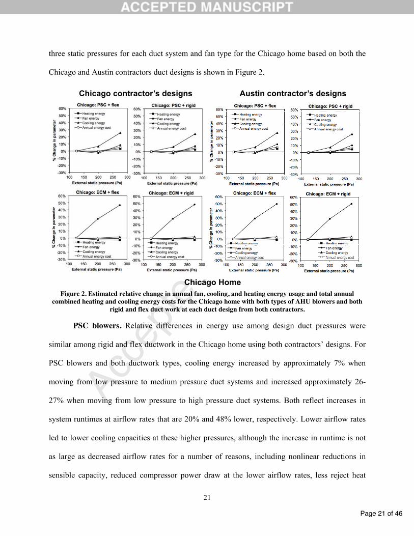
The relative comparison of annual (i) heating energy, (ii) fan energy, (iii) cooling energy,

and (iv) total HVAC energy costs estimated for the baseline (present) year between each of the

of 46

Accep

ted M

anus

cript

21

three static pressures for each duct system and fan type for the Chicago home based on both the

Chicago and Austin contractors duct designs is shown in Figure 2.

Austin contractor’s designs Chicago contractor’s designs

Figure 2. Estimated relative change in annual fan, cooling, and heating energy usage and total annual

combined heating and cooling energy costs for the Chicago home with both types of AHU blowers and both rigid and flex duct work at each duct design from both contractors.

PSC blowers. Relative differences in energy use among design duct pressures were

similar among rigid and flex ductwork in the Chicago home using both contractors’ designs. For

PSC blowers and both ductwork types, cooling energy increased by approximately 7% when

moving from low pressure to medium pressure duct systems and increased approximately 26-

27% when moving from low pressure to high pressure duct systems. Both reflect increases in

system runtimes at airflow rates that are 20% and 48% lower, respectively. Lower airflow rates

led to lower cooling capacities at these higher pressures, although the increase in runtime is not

as large as decreased airflow rates for a number of reasons, including nonlinear reductions in

sensible capacity, reduced compressor power draw at the lower airflow rates, less reject heat

Chicago Home

of 46

Accep

ted M

anus

cript

22

added to the airstream for the PSC blowers, and lower conductive losses through ductwork with

typically lower surface areas and thus lower UA values.

Annual fan energy did not change when moving from low to medium pressure scenarios

with the Chicago contractor’s duct designs but decreased 2% with the Austin contractor’s

designs. Annual fan energy then increased by 11-14% when moving to the highest pressure

PSC+flex system, suggesting that any reductions in fan power draw observed at moderately

increased static pressures were overwhelmed by longer system runtimes. Similar changes of -1%

and +10-11% were also predicted for the PSC+rigid system. Annual heating energy increased 3-

5% for both PSC+flex and PSC+rigid systems at the highest pressures using both contractors’

designs; changes in heating energy were negligible for the medium pressure systems.

Total HVAC energy costs in the baseline year were estimated to be between ~0.2% lower

and 0.4% higher for each of the PSC+flex scenarios with medium pressure ducts compared to

low pressure ducts (the same medium pressure comparison resulted in baseline HVAC energy

costs between 0.2% and 1.6% higher for PSC+rigid scenarios, depending on contractor design).

Total HVAC energy costs in the baseline year for the high pressure PSC+flex duct systems were

estimated to be between 5.4% and 6.9% higher compared to the low pressure systems (again

depending on contractor design), and between 5.1% and 6.7% higher for the high pressure

PSC+rigid systems. Overall, these results suggest that for PSC blowers in this home, the use of

the lowest pressure duct designs could likely save approximately 5-7% in total annual HVAC

energy costs relative to the highest pressure designs.

ECM blowers. For the ECM+flex system, there were only small increases in cooling

energy consumption of 0% and +2-3% at medium and high pressures relative to low pressures,

respectively, which is generally appropriate for very small changes in airflow rates and cooling

of 46

Accep

ted M

anus

cript

23

capacities (from Table 2). The slight increase in cooling energy at the highest pressure may be

explained by an increase in heat rejected into the airstream by the ECM blowers using more

power. There was a 27-29% and 47-50% increase in fan energy consumption for the two higher

pressures, respectively, using both contractors’ designs with ECM+flex combinations, due

primarily to greater power draw of the ECM blowers at higher pressures. There was also a 1-3%

reduction in heating energy at these higher pressures, likely due to the combination of increased

reject heat from the fans as they drew more power at higher pressures, as well as a small

reduction in conductive losses through lower UA ducts (particularly for the Chicago contractor’s

designs). Similarly for the ECM+rigid systems, cooling energy increased 0-1% and 3-4% at

medium and high pressures relative to the low pressure designs; fan energy increased 28-29%

and 48-50%, and heating energy decreased as much as 2% (Chicago contractor) or as little as 0%

(Austin contractor) at each of the same pressures. This difference is likely due to the fact that for

the Chicago home, the average total duct UA values across all scenarios was approximately 73%

greater with the Chicago contractor’s duct designs than the Austin contractor’s designs (average

of 120 W/K vs. 70 W/K).

Differences in HVAC energy costs in the baseline year for the ECM scenarios were

smaller than the PSC scenarios. Total HVAC energy costs were 0.2-1% lower for the medium

pressure ECM+flex systems and between 0.2% lower and 1.2% higher for the medium pressure

ECM+rigid systems, depending on contractor design. Total HVAC energy costs were between

0.3% lower and 1.6% higher for the high pressure ECM+flex combinations and 0.8-2.4% higher

in the high pressure ECM+rigid combinations.

of 46

Accep

ted M

anus

cript

24

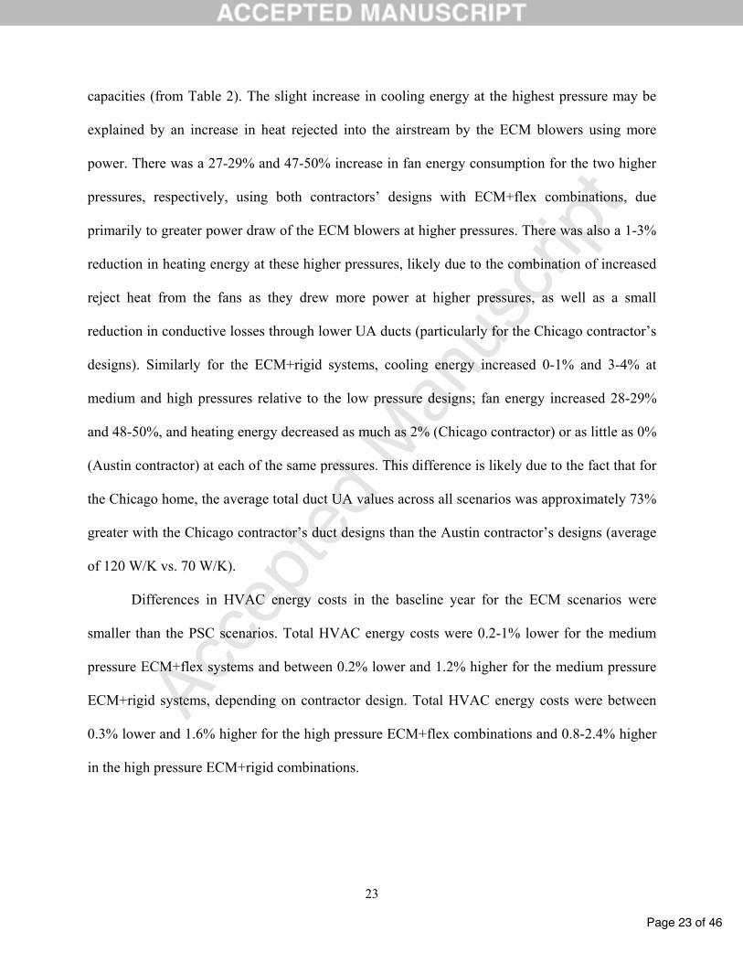
4.2.2 Austin home energy simulations

The relative comparison of annual (i) heating energy, (ii) fan energy, (iii) cooling energy,

and (iv) total HVAC energy costs in the baseline year between each of the three static pressures

for each duct system and fan type for the Austin home based on both the Chicago and Austin

contractors duct designs is similarly shown in Figure 3.

Austin contractor’s designs Chicago contractor’s designs

Figure 3. Estimated relative change in annual fan, cooling, and heating energy usage and total annual

combined heating and cooling energy costs for the Austin home with both types of AHU blowers and both rigid and flex duct work at each duct design from both contractors.

PSC blowers. In the Austin home with PSC blowers and flexible ductwork materials,

cooling energy slightly decreased by 0.3% when moving from low pressure to medium pressure

designs by the Chicago contractor but increased ~5% using the Austin contractor’s designs.

Again the difference stems from large differences in duct UA values in unconditioned space,

which varied highly between the two contractors. When moving from low pressure to high

Austin Home

of 46

Accep

ted M

anus

cript

25

pressure duct designs with PSC+flex systems, cooling energy increased by 14% to 18%,

depending on contractor designs. The same impacts were greater in magnitude for the PSC+rigid

combinations: cooling energy increased 3-4% at medium pressures and increased 17-20% at high

pressures. Again, increases in cooling energy were due to a combination of longer system

runtimes mitigated in part by a lower fan power draw (which rejects less heat into the airstream),

lower compressor power draw, and reduced heat transfer across ductwork surfaces at the higher

pressure designs.

Annual fan energy decreased 15% and 11% with PSC+flex combinations when moving

from low to medium pressure with the Chicago and Austin contractors’ designs, respectively.

Annual fan energy decreased 23-25% with the same combination when moving from the low to

high pressure designs, depending on contractor design. Results were similar for the PSC+rigid

systems (12-13% reductions for medium pressures and 22-23% for the lowest pressures). Annual

heating energy consumption increased 5-9% and 11-12% for both PSC+flex and PSC+rigid

systems at the medium pressures using the Chicago and Austin contractors’ designs,

respectively. More substantially, annual heating energy consumption increased 43-54% with the

highest pressure Chicago contractor’s PSC+flex and PSC+rigid designs and 49-50% with the

highest pressure Austin contractor’s PSC+flex and PSC+rigid designs.

Total HVAC energy costs in the baseline year were 1% lower and 19% higher for the

medium and high pressure PSC+flex combinations compared to their low pressure counterparts,

respectively, and 2% and 25% higher for the medium and high pressure PSC+rigid

combinations, respectively, all with the Chicago contractor’s designs. Similarly, total HVAC

energy costs in the baseline year were 5% higher and 23% higher for the medium and high

pressure PSC+flex combinations compared to low pressure designs, respectively, and 4% and

of 46

Accep

ted M

anus

cript

26

22% higher for the medium and high pressure PSC+rigid combinations, respectively, when using

the Austin contractor’s designs in the Austin home. Therefore, the lowest pressure duct designs

in this home with a PSC blower could lead to substantial reductions in HVAC energy costs (as

much as 22-25%) relative to those encountered using the highest pressure duct designs. Moderate

pressure designs had a smaller impact, but still led to 2-5% higher heating and cooling energy

consumption relative to the lowest pressures.

ECM blowers. For the ECM+flex systems using the Chicago contractor’s designs, there

was a 6% increase in cooling energy consumption at both medium and high pressures, which

captures the combined effects of excess heat rejected to the airstream by the AHU blowers

drawing more power at greater pressures offset some by lower duct UA values. However, there

was no observable change in cooling energy consumption at either pressure with the ECM+flex

systems using the Austin contractor’s designs, likely due to small changes in duct UA values

with their designs. Annual fan energy increased by 25-32% and 46-55% for the medium and high

pressure ECM+flex designs, respectively, depending on contractor designs. There was also a 9%

and 2-3% reduction in heating energy at both of these higher pressures with the Chicago and

Austin contractor designs, respectively, most likely due to the combined effects of reduced heat

transfer across the lower UA ductwork designs in the unconditioned attic and the addition of

excess reject heat from the fans drawing higher power at higher pressures. Similarly for the

ECM+rigid systems, cooling energy decreased by 1-2% at both medium and high pressures

relative to the lowest pressure; fan energy increased 29-30% and 50-54%; and heating energy

decreased 3-5% at each of the same pressures, depending on contractor designs. Again,

differences in total HVAC energy costs in the baseline year for the ECM scenarios were smaller

than the PSC scenarios.

of 46

Accep

ted M

anus

cript

27

4.3 Life cycle cost analysis

Although the single-year annual simulation results above are helpful for interpreting

energy usage and operational cost impacts of each duct design and blower combination, a life

cycle analysis was also conducted to determine the true cost-benefit relationship between

differences in initial costs among duct configurations and subsequent increases or decreases in

HVAC energy costs. The NPV estimates are explored first by comparing both the medium and

low system pressure conditions against the highest-pressure condition for each house and blower

type and treating (1) flex duct systems and (2) rigid duct systems separately. Blower types and

results from the Chicago and Austin contractors’ duct designs and cost estimates are also treated

separately. Flex and rigid duct systems are treated separately to limit the cost comparisons to the

impacts of duct pressures alone (which is the main focus of this study). Additionally,

comparisons across ductwork types are not always appropriate. For example, in the City of

Chicago, flexible nonmetallic ductwork is not permitted in residential units per the building

code, §18-28-603. In other settings, it may be standard industry practice for contractors to rely

exclusively on flexible ductwork and thus rigid duct designs may seldom be used. However, one

final comparison involved exploring the same data and the same division of blower types but

also comparing the medium and low pressure systems with both flex duct and rigid sheet metal

duct materials to the highest-pressure flex condition in each case. This procedure allows for a life

cycle cost comparison across duct materials (i.e., of flex vs. rigid), although it is limited to

several important assumptions and limitations outlined in the accompanying text in that section.

4.3.1 NPV analysis assuming 15-year life cycle: Flex duct only

In the NPV calculation procedure, we assumed that the entire cost of duct design and

installation was incurred in the initial year (year 0). Subsequently, the total annual electricity

of 46

Accep

ted M

anus

cript

28

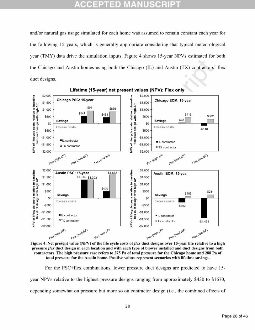
and/or natural gas usage simulated for each home was assumed to remain constant each year for

the following 15 years, which is generally appropriate considering that typical meteorological

year (TMY) data drive the simulation inputs. Figure 4 shows 15-year NPVs estimated for both

the Chicago and Austin homes using both the Chicago (IL) and Austin (TX) contractors’ flex

duct designs.

$541 $431

$911 $836

-$2,000

-$1,500

-$1,000

-$500

$0

$500

$1,000

$1,500

$2,000

Flex (high ǻP)

Flex (med ǻP)

Flex (low ǻP)

NP

V o

f life

cycl

e co

sts

rela

tive

to b

asel

ine

flex

duct

des

ign

with

hig

h ǻ

P

Chicago PSC: 15-year

IL contractor

TX contractor

$37

-$148

$419 $302

-$2,000

-$1,500

-$1,000

-$500

$0

$500

$1,000

$1,500

$2,000

Flex (high ǻP)

Flex (med ǻP)

Flex (low ǻP)

NP

V o

f life

cycl

e co

sts

rela

tive

to b

asel

ine

flex

duct

des

ign

with

hig

h ǻ

P

Chicago ECM: 15-year

IL contractor

TX contractor

$1,314

$490

$1,303

$1,672

-$2,000

-$1,500

-$1,000

-$500

$0

$500

$1,000

$1,500

$2,000

Flex (high ǻP)

Flex (med ǻP)

Flex (low ǻP)

NP

V of

life

cycl

e co

sts

rela

tive

to b

asel

ine

flex

duct

des

ign

with

hig

h ǻ

P

Austin PSC: 15-year

IL contractor

TX contractor

-$302

-$1,435

$109 $241

-$2,000

-$1,500

-$1,000

-$500

$0

$500

$1,000

$1,500

$2,000

Flex (high ǻP)

Flex (med ǻP)

Flex (low ǻP)

NP

V of

life

cycl

e co

sts

rela

tive

to b

asel

ine

flex

duct

des

ign

with

hig

h ǻ

P

Austin ECM: 15-year

IL contractor

TX contractor

Excess costs Savings




Lifetime (15-year) net present values (NPV): Flex only

Figure 4. Net present value (NPV) of the life cycle costs of flex duct designs over 15-year life relative to a high pressure flex duct design in each location and with each type of blower installed and duct designs from both

contractors. The high pressure case refers to 275 Pa of total pressure for the Chicago home and 288 Pa of total pressure for the Austin home. Positive values represent scenarios with lifetime savings.

For the PSC+flex combinations, lower pressure duct designs are predicted to have 15-

year NPVs relative to the highest pressure designs ranging from approximately $430 to $1670,

depending somewhat on pressure but more so on contractor design (i.e., the combined effects of

of 46

Accep

ted M

anus

cript

29

initial cost estimates and duct UA values based on individual designs). For the Chicago

contractor’s designs, the medium pressure PSC+flex combination yielded the highest NPV; for

the Austin contractor’s PSC+flex combinations, the lowest pressure PSC+flex combination

yielded the highest NPV in the Austin home and was similar to the medium pressure results in

the Chicago home.

For ECM+flex systems, 15-year NPVs of lower pressure scenarios ranged from a savings

of $37 to an excess cost of $1435 with the Chicago contractor’s designs. The Austin contractor’s

designs yielded savings in all lower pressure scenarios ranging from $109 to $419, again with the

medium pressure duct system in the Chicago home having a higher NPV than the low pressure

system and vice versa in the Austin home. These results suggest that within flexible duct systems

only, both medium and low pressure duct systems can generally yield life cycle costs savings

over a 15-year period, particularly for PSC systems and often for ECM systems, although the

savings are not as large as with PSC blowers and may vary depending on actual duct designs and

costs.

To provide a more concise summary of these results, Table 5 also summarizes these

results using a simple nomenclature, whereby a positive NPV for a scenario (i.e., a scenario with

life cycle cost savings) is marked with a positive sign (+) and scenarios with excess life cycle

costs are marked with a negative sign (-).

Table 5. Summary of 15-year NPV analysis for flex ducts only 15-year NPV relative to high pressure flex1 Home Contractor Blower Flex low Flex medium

PSC + + IL ECM - + PSC + + Chicago

TX ECM + + PSC + + IL ECM - - PSC + + Austin

TX ECM + + Number of scenarios w/ savings: 6/8 7/8

of 46

Accep

ted M

anus

cript

30

1Positive signs (+) reflect life cycle cost savings. Negative signs (-) reflect excess life cycle costs.

According to Table 5, the lower pressure flex duct designs reflect life cycle cost savings

over the high pressure flex designs in most of the modeled scenarios: six out of eight scenarios

for the lowest pressure flex systems and seven out of eight scenarios for the medium pressure

flex duct systems.

4.3.2 NPV analysis assuming 15-year life cycle: Rigid ducts only

Similar to the analysis for flex duct designs only above, Figure 5 shows 15-year NPVs of

lower pressure designs relative to the highest pressure designs estimated for the Chicago and

Austin homes using both the Chicago (IL) and Austin (TX) contractors’ rigid duct designs. Table

6 also summarizes these same data using the simplified “+/-” nomenclature used in the previous

summaries.

of 46

Accep

ted M

anus

cript

31

$351

-$1,124

$460 $671

-$2,000

-$1,500

-$1,000

-$500

$0

$500

$1,000

$1,500

$2,000

Flex (high ǻP)

Flex (med ǻP)

Flex (low ǻP)

NPV

of l

ifecy

cle

cost

s re

lativ

e to

bas

elin

e fle

x du

ct d

esig

n w

ith h

igh ǻ

P


IL contractor

TX contractor

-$36

-$1,540

$64 $244

-$2,000

-$1,500

-$1,000

-$500

$0

$500

$1,000

$1,500

$2,000

Flex (high ǻP)

Flex (med ǻP)

Flex (low ǻP)

NPV

of l

ifecy

cle

cost

s re

lativ

e to

bas

elin

e fle

x du

ct d

esig

n w

ith h

igh ǻ

P


IL contractor

TX contractor

$1,328

$991

$1,377 $1,510

-$2,000

-$1,500

-$1,000

-$500

$0

$500

$1,000

$1,500

$2,000

Flex (high ǻP)

Flex (med ǻP)

Flex (low ǻP)

NP

V of

life

cycl

e co

sts

rela

tive

to b

asel

ine

flex

duct

des

ign

with

hig

h ǻ

P

Austin PSC: 15-year

IL contractor

TX contractor

-$297

-$784

$161 $70

-$2,000

-$1,500

-$1,000

-$500

$0

$500

$1,000

$1,500

$2,000

Flex (high ǻP)

Flex (med ǻP)

Flex (low ǻP)

NP

V of

life

cycl

e co

sts

rela

tive

to b

asel

ine

flex

duct

des

ign

with

hig

h ǻ

P

Austin ECM: 15-year

IL contractor

TX contractor

Lifetime (15-year) net present values (NPV): Rigid only





Figure 5. Net present value (NPV) of the life cycle costs of rigid duct designs over 15-year life relative to a

high pressure rigid duct design in each location and with each type of blower installed and duct designs from both contractors. The high pressure case refers to 275 Pa of total pressure for the Chicago home and 288 Pa

of total pressure for the Austin home. Positive values represent scenarios with lifetime savings. Table 6. Summary of 15-year NPV analysis for rigid ducts only

15-year NPV relative to high pressure rigid1 Home Contractor Blower Rigid low Rigid medium

PSC - + IL ECM - - PSC + + Chicago

TX ECM + + PSC + + IL ECM - - PSC + + Austin

TX ECM + + Number of scenarios w/ savings: 5/8 6/8

1Positive signs (+) reflect life cycle cost savings. Negative signs (-) reflect excess life cycle costs.

Limiting life cycle cost comparisons to within rigid systems alone, the lower pressure

rigid duct designs also reflect life cycle cost savings over the high pressure rigid designs in the

of 46

Accep

ted M

anus

cript

32

majority of modeled scenarios: five out of eight scenarios for the lowest pressure rigid systems

and six out of eight scenarios for the medium pressure rigid duct systems. This is particularly

true for PSC blowers, but also for some ECM scenarios. However, the magnitude (and

sometimes direction) of savings changed depending on blower type, level of pressure, and details

of individual contractor duct designs and initial cost estimates. For example, all of the lower

pressure duct designs from the Austin contractor yielded life cycle cost savings (ranging from

$460 to $1510 for PSC+rigid combinations and from $64 to $244 for ECM+rigid combinations).

The only scenarios that did not yield life cycle savings were those using the Chicago contractor’s

designs and estimates. ECM scenarios using the Chicago contractor’s designs yielded excess life

cycle costs in both homes and only one PSC scenario (low pressure in the Chicago home with

the Chicago contractor’s designs) is expected to yield excess life cycle costs. This was due to a

combination of excess ductwork costs and higher duct UA values using only the Chicago

contractor’s designs; the Austin contractor’s designs did not reflect such dramatic changes in

upfront costs or duct UA. Details of individual contractor designs thus can have a very large

impact on the economics of lower pressure duct systems in residences.

Overall, these results suggest that within the constraints of using rigid duct materials, low

pressure duct systems can generally yield life cycle cost savings in systems with PSC blowers

(i.e., up to ~$1500), depending on contractor design characteristics and upfront costs. In systems

with ECM blowers, lower pressure duct systems can either yield slight life cycle cost savings or

as much as ~$1500 in excess life cycle costs in these two homes, depending primarily on

contractor cost estimates and design characteristics.

of 46

Accep

ted M

anus

cript

33

4.3.3 15-year NPV analysis: Comparing both flex and rigid duct scenarios

There are also cases where one may have the option to select either flexible or rigid metal

duct materials. Therefore, we have provided an additional life cycle cost comparison of each of

the modeled scenarios comparing across both flex and rigid duct materials, all referenced to what

was originally expected to be the least expensive initial cost scenario: the highest pressure flex

condition. Figure 6 and Figure 7 show 15-year NPVs calculated for each of the Chicago and

Austin contractors’ duct designs and cost estimates, respectively. Both the medium and low

pressure flex designs, as well as the low, medium, and high pressure rigid designs, are compared

to the highest pressure flex duct design in this analysis. Positive values again indicate scenarios

that yield net savings over an assumed 15-year lifetime. Importantly, this analysis assumes that

each duct type is equally capable of achieving the target pressures specified. In reality, flexible

ductwork materials are much more likely to be constricted during construction due to installation

with excessive compression, excessive sag, or being pinched by wires and cables. Therefore

these results should be interpreted with some caution.

of 46

Accep

ted M

anus

cript

34

0 $541 $431

-$3,559 -$3,208

-$4,683

-$8,000

-$6,000

-$4,000

-$2,000

$0

$2,000

$4,000

Flex (high ǻP)

Flex (med ǻP)

Flex (low ǻP)

Metal (high ǻP)

Metal (med ǻP)

Metal (low ǻP)

NPV

of l

ifecy

cle

cost

s re

lativ

e to

bas

elin

e fle

x du

ct d

esig

n w

ith h

igh ǻ

P


0 $37

-$148

-$3,746 -$3,788

-$5,293

-$8,000

-$6,000

-$4,000

-$2,000

$0

$2,000

$4,000

Flex (high ǻP)

Flex (med ǻP)

Flex (low ǻP)

Metal (high ǻP)

Metal (med ǻP)

Metal (low ǻP)

NPV

of l

ifecy

cle

cost

s re

lativ

e to

bas

elin

e fle

x du

ct d

esig

n w

ith h

igh ǻ

P


0

$1,314 $490

-$3,922

-$2,595 -$2,932

-$8,000

-$6,000

-$4,000

-$2,000

$0

$2,000

$4,000

Flex (high ǻP)

Flex (med ǻP)

Flex (low ǻP)

Metal (high ǻP)

Metal (med ǻP)

Metal (low ǻP)

NPV

of l

ifecy

cle

cost

s re

lativ

e to

bas

elin

e fle

x du

ct d

esig

n w

ith h

igh ǻ

P

Austin PSC: 15-year

0

-$302

-$1,435

-$4,193 -$4,490 -$4,977

-$8,000

-$6,000

-$4,000

-$2,000

$0

$2,000

$4,000

Flex (high ǻP)

Flex (med ǻP)

Flex (low ǻP)

Metal (high ǻP)

Metal (med ǻP)

Metal (low ǻP)

NPV

of l

ifecy

cle

cost

s re

lativ

e to

bas

elin

e fle

x du

ct d

esig

n w

ith h

igh ǻ

P

Austin ECM: 15-year

Lifetime (15-year) net present values (NPV) using the Chicago contractor’s duct designs

Excess costs

Savings

Excess costs

Savings

Excess costs

Savings

Excess costs

Savings

Figure 6. Net present value (NPV) of the life cycle costs of both flex and rigid duct designs over 15-year life relative to the high pressure flex duct condition in each location and with each type of blower installed. Duct

designs are limited only to the Chicago contractor’s for clarity. The high pressure case refers to 275 Pa of total pressure for the Chicago home and 288 Pa of total pressure for the Austin home. Positive values

represent scenarios with life cycle cost savings.

of 46

Accep

ted M

anus

cript

35

0 $911 $836

-$3,200 -$2,740 -$2,529

-$8,000

-$6,000

-$4,000

-$2,000

$0

$2,000

$4,000

Flex (high ǻP)

Flex (med ǻP)

Flex (low ǻP)

Metal (high ǻP)

Metal (med ǻP)

Metal (low ǻP)

NPV

of l

ifecy

cle

cost

s re

lativ

e to

bas

elin

e fle

x du

ct d

esig

n w

ith h

igh ǻ

P


0 $419 $302

-$3,321 -$3,264 -$3,092

-$8,000

-$6,000

-$4,000

-$2,000

$0

$2,000

$4,000

Flex (high ǻP)

Flex (med ǻP)

Flex (low ǻP)

Metal (high ǻP)

Metal (med ǻP)

Metal (low ǻP)

NPV

of l

ifecy

cle

cost

s re

lativ

e to

bas

elin

e fle

x du

ct d

esig

n w

ith h

igh ǻ

P


0

$1,303 $1,672

-$2,915

-$1,538 -$1,405

-$8,000

-$6,000

-$4,000

-$2,000

$0

$2,000

$4,000

Flex (high ǻP)

Flex (med ǻP)

Flex (low ǻP)

Metal (high ǻP)

Metal (med ǻP)

Metal (low ǻP)

NPV

of l

ifecy

cle

cost

s re

lativ

e to

bas

elin

e fle

x du

ct d

esig

n w

ith h

igh ǻ

P

Austin PSC: 15-year

0 $109 $241

-$2,911 -$2,749 -$2,840

-$8,000

-$6,000

-$4,000

-$2,000

$0

$2,000

$4,000

Flex (high ǻP)

Flex (med ǻP)

Flex (low ǻP)

Metal (high ǻP)

Metal (med ǻP)

Metal (low ǻP)

NPV

of l

ifecy

cle

cost

s re

lativ

e to

bas

elin

e fle

x du

ct d

esig

n w

ith h

igh ǻ

P

Austin ECM: 15-year

Lifetime (15-year) net present values (NPV) using the Austin contractor’s duct designs

Excess costs

Savings

Excess costs

Savings

Excess costs

Savings

Excess costs

Savings

Figure 7. Net present value (NPV) of the life cycle costs of both flex and rigid duct designs over 15-year life relative to the high pressure flex duct condition in each location and with each type of blower installed. Duct designs are limited only to the Austin contractor’s for clarity. The high pressure case refers to 275 Pa of total

pressure for the Chicago home and 288 Pa of total pressure for the Austin home. Positive values represent scenarios with life cycle cost savings.

Table 7 summarizes these results comparing both ductwork materials for both homes

with designs from both contractors using the same simple nomenclature as in previous sections.

Again, most of the medium and low pressure flex duct designs are predicted to yield life cycle

cost savings relative to the high pressure flex designs across both homes and both contractor

designs. Six out of eight low pressure flex duct scenarios are expected to yield life cycle cost

savings while seven out of eight medium pressure flex duct scenarios are expected to yield

Excess costs

of 46

Accep

ted M

anus

cript

36

savings. These results are the same as the flex only section above. However, in this analysis none

of the rigid duct scenarios are expected to yield life cycle savings; their initial cost estimates

from both contractors are too high relative to any expected annual HVAC energy cost savings.

These results suggest that for this particular home in this particular climate and under the

assumptions described herein, lower pressure duct designs yield 15-year life cycle savings only

for flexible ductwork. Switching to rigid ductwork and assuming that the target pressures can be

met does not yield life cycle cost savings because of very high upfront costs. However, as

mentioned, this analysis is limited to the assumption that both ductwork materials are equally

likely to achieve the desired pressures.

Table 7. Summary of 15-year NPV analysis for both flex and rigid ductwork 15-year NPV relative to high pressure flex1

Home Contractor Blow

er Flex low

Flex medium

Rigid low

Rigid medium

Rigid high

PSC + + - - - Chicago

ECM - + - - - PSC + + - - -

Chicago Austin

ECM + + - - - PSC + + - - -

Chicago ECM - - - - - PSC + + - - -

Austin Austin

ECM + + - - - Number of scenarios w/ savings: 6/8 7/8 0/8 0/8 0/8

1Positive signs (+) reflect positive NPVs (i.e., life cycle cost savings). Negative signs (-) reflect excess life cycle costs.

5. Discussion

There were a total of 48 scenarios modeled herein, which complete a simulation matrix

comprising two contractors’ duct designs, two model homes, two types of blowers, two types of

duct materials, and three levels of duct pressures. If flexible and rigid duct materials are treated

separately, sixteen of these simulations represent baseline highest pressure duct designs, leaving

a total of 32 lower pressure comparison scenarios. In the Chicago home with flexible ductwork,

of 46

Accep

ted M

anus

cript

37

the lower pressure scenario that provided the greatest life cycle cost savings (highest NPV)

relative to the highest pressure scenario was that with a PSC blower operating at medium

pressure using the Austin contractor’s designs ($911). The lowest pressure PSC scenario with the

Austin contractor’s designs yielded the next largest cost savings ($836). In the same home with

rigid ductwork, the lowest pressure PSC scenario with the Austin contractor’s designs yielded

the greatest life cycle cost savings (highest NPV) ($671). Three of the four lower pressure PSC

scenarios using the Chicago contractor’s designs actually yielded excess life cycle costs (as

much as $1540 more), suggesting again that design details and cost estimates play an important

role in the life cycle cost impacts of lower pressure duct designs.

In the Austin home with flexible ductwork, the lower pressure scenario that provided the

greatest life cycle cost savings relative to the highest pressure scenario was that with a PSC

blower operating at the lowest pressure using the Austin contractor’s designs ($1672). The

medium pressure PSC scenarios with either contractor’s designs provided the next largest

savings (around $1300). Again, results of lower pressure scenarios with the Chicago contractor’s

designs and cost estimates were more variable, sometimes providing savings (as much as $1300)

and sometimes yielding excess life cycle costs (as much as $1400). In the same home with rigid

sheet metal ductwork, the lowest pressure PSC scenario with the Austin contractor’s designs

again yielded the greatest life cycle cost savings ($1510), with the medium pressure scenario and

the Austin contractor’s designs not far behind ($1377). Results with the Chicago contractor’s

estimates were again more variable, with savings as large as $1328 and excess life cycle costs as

high as $784.

Taken together, these results suggest that either medium or low pressure flex duct

systems are generally preferred from a life cycle cost perspective in these two homes with either

of 46

Accep

ted M

anus

cript

38

contractor’s designs, particularly if a PSC blower is installed, and that the magnitude (and

sometimes direction) of savings will depend mostly on individual contractor duct designs and

cost estimates. These savings are predicted primarily because the lower pressure designs allow

for the HVAC systems to maintain adequate airflow rates and operate for shorter periods of time

over the course of a year.

5.1 Sensitivity

Changes in a number of assumptions in this work may have led to very different results

and conclusions. For example, changes in assumptions for future energy costs, duct leakage

fractions, ductwork insulation values, thermostat set points, envelope thermal performance,

HVAC equipment efficiency (i.e., SEER for both air-conditioning units, AFUE for the furnace,

and HSPF for the heat pump), HVAC equipment and ductwork lifespans, and the location of the

ductwork (i.e., moving inside to conditioned space), can all have a large impact on the simulation

results. However, it was beyond the scope of this project to systematically vary each parameter

individually as would be appropriate for a large suite of Monte Carlo simulations, so we rely

primarily on a qualitative discussion of the sensitivity to these important parameters with some

quantitative approximations of one particular influence.

For one, if future energy costs for either natural gas or electricity were to increase at a

greater rate than what is modeled herein, the predicted annual savings in energy costs for each of

the lower pressure duct scenarios would be larger and would thus yield larger life cycle savings

relative to the baseline high pressure flex conditions. Depending on the increase in energy costs

this could potentially increase the number of scenarios with life cycle cost savings. Similar

impacts would be seen if other inputs that affect the absolute amount of energy used for space

conditioning were also varied, including higher thermostat settings in the winter, lower

of 46

Accep

ted M

anus

cript

39

thermostat settings in the summer, decreased envelope performance, and decreased HVAC

equipment efficiency. Conversely, lower thermostat settings in the winter, higher thermostat

settings in the summer, improved envelope performance, increased HVAC equipment efficiency,

and moving ducts into conditioned space would all work to decrease annual energy demands and

thus make differences between scenarios even smaller, which could potentially decrease the

number of scenarios in which positive NPVs are observed.

As an example of the potential of these effects, we explored how the results may vary

with one particularly important set of input parameters: HVAC equipment efficiency. The

modeled homes relied on SEER 15 air-conditioning units (both homes), a heat pump with 8.5

HSPF (Austin), and a gas furnace with 92.5 AFUE (Chicago). If the efficiency of the air-

conditioning units was decreased to SEER 13, the HSPF was decreased to 7.7, and the furnace

was decreased to AFUE 80, which are each more in line with code minimums in most locations,

then the modeled homes would be expected to use approximately 15% more energy for cooling

in both homes and 10% and 16% more energy for heating in the Austin and Chicago homes,

respectively, using a simple comparison of nominal COP values. Systems would not run longer

because the loads would not change; only the amount of energy required to meet the same loads

would change at each time step. This simple linear approximation was verified using only one

altered simulation case. Using these simple differences, although the magnitude of savings

changed by as much as about $250 in terms of 15-year NPV, the number of simulation cases

resulting in life cycle cost savings did not change, suggesting that the summary of results herein

is not impacted significantly by these assumptions for input parameters. Other variations in input

parameters may have different impacts but are not explored in this work.

of 46

Accep

ted M

anus

cript

40

A final important assumption to explore is the use of a 15-year life cycle in our NPV

calculations. A 15-year timeline was used because although duct systems are expected to last

much longer, these simulations rely on accurate assumptions for HVAC equipment efficiency.

Typical HVAC equipment lifespans are in the range of 15 years, so it is very likely that in the

lifespan of a duct system, some or all HVAC equipment components would be replaced.

However, there is no way of knowing what efficiency equipment will be available on the market

15 years from now, let alone what their upfront costs may be. Therefore, we simply explored the

sensitivity of our results to the assumption of life cycle length by repeating our analyses with a

30-year life cycle. Importantly, adjusting to a 30-year lifespan did not drastically change the

direction of most results herein. In fact, only one scenario (the PSC+rigid medium pressure

design in the Chicago home using the Chicago contractor’s designs) moved from a net excess

cost to a slight net savings. The magnitude of savings did however increase over time for most

scenarios. These results suggest that the assumed timeframe does not have a large impact on this

analysis in these homes and under all of the underlying assumptions used herein.

5.2 Limitations

There are a number of important limitations to this work that should be mentioned. For

one, this work was limited to the particular homes, climates, duct designs, cost estimates, and

choices of input parameters used herein. Results may not be extrapolated directly to other

environments. Second, this work did not capture any changes in system pressures over time;

pressures were assumed constant throughout the year. Third, this work assumed that both

flexible and rigid sheet metal ductwork have the same likelihood of being installed according to

industry quality standards and therefore can meet the specified design pressures. In reality,

flexible ductwork materials are more likely to be constricted during construction due to

of 46

Accep

ted M

anus

cript

41

installation with excessive compression, excessive sag, or being pinched by wires and cables.

However, these impacts were not captured herein. Fourth, this work focused only on energy

consumption impacts and did not explore other factors such as air distribution effectiveness,

occupant comfort, indoor air quality, or noise. Finally, this work did not explore differences in

equipment reliability and maintenance that may differ across the ductwork materials used or

between the two blower types. For example, blower motors may need to be replaced more often

when subjected to excessive static pressures, but we are not aware of accurate ways to estimate

replacement times under different operational conditions and thus these impacts remain beyond

the scope of this study. Future work should systematically explore the sensitivity of these results

and conclusions to deviations from a number of important input parameters and assumptions

used herein.

6. Conclusions

It is commonly assumed that lower pressure duct systems are preferred for use in central

residential heating and air-conditioning systems because they will result in greater airflow rates

and cooling and heating capacities with PSC blowers and lower fan power draws with ECM

blowers. Results from the 48 annual building energy simulations and life cycle cost analyses

using a number of blower types, ductwork materials, and duct designs meeting a range of

specified external static pressures in the two model homes described herein suggest the

following:

1. Lower airflow rates and heating and cooling capacities caused by excessive system

pressures (e.g., total external static pressures of 275-288 Pa) introduced by duct designs

with high static pressures in the model homes with PSC blowers yielded substantial

of 46

Accep

ted M

anus

cript

42

increases in HVAC energy use compared to the same systems operating with lower

pressure duct designs (e.g., total external static pressures of 125-138 Pa).

2. HVAC energy impacts of the same systems using ECM blowers were not as large as

those using PSC blowers because although ECM blowers draw more power to maintain

nearly constant airflow rates and heating and cooling capacities at higher pressure drops,

fan power was a small portion of the overall HVAC energy use.

3. When the initial costs of lower pressure duct designs were taken into account over a 15-

year or 30-year life cycle, lower pressure duct designs generally yielded life cycle cost

savings relative to the highest pressure duct systems, particularly in homes with PSC

blowers and particularly when making comparisons with constant ductwork materials

(i.e., comparing flex only or rigid only).

4. Lower pressure duct designs combined with ECM blowers can also yield life cycle cost

savings over the highest pressure duct designs, although the magnitude of savings was

typically lower than with PSC blowers and varied depending on specific duct design

details and contractor cost estimates.

5. Specific details in contractor duct designs and cost estimates intended to meet specific

external static pressures can have a large influence on the impacts that ductwork designs

can have on HVAC energy consumption and total life cycle costs in residences.

Acknowledgements

This work was funded by the Air-Conditioning, Heating, and Refrigeration Institute

(AHRI Project No. 8002). We are grateful for the AHRI project monitoring committee for their

helpful comments throughout the project and for Jon Lemmond and Xudong Wang for their

work as project facilitators within AHRI. I would also like to acknowledge Zeineb El Orch for

of 46

Accep

ted M

anus

cript

43

her tireless efforts in performing much of the energy simulations and cost analyses herein and

Hailey Kunkel for her work translating duct designs into a format for use in the energy modeling.

Finally, I would also like to acknowledge the work of Robert Doornbos at Doornbos Heating and

Air Conditioning in Chicago, IL and Chris Henderson and staff at Austin Air Conditioning, Inc.,

in Austin TX for their work on the duct designs and cost estimates used herein.

References

[1] DOE, Test Procedure for Residential Central Air Conditioners and Heat Pumps: Final Rule, Federal Register 70 (195), 59122-59180, Part II. 10 CFR Part 430, Energy Conservation Program for Consumer Products, 2005.

[2] ASHRAE, Chapter 16: Duct Construction, in: 2004 ASHRAE Handbook—HVAC Systems and Equipment, American Society of Heating, Refrigerating and Air-Conditioning Engineers, Inc, Atlanta, GA, 2004.

[3] J. Lutz, V. Franco, A. Lekov, G. Wong-Parodi, BPM Motors in Residential Gas Furnaces: What are the Savings?, in: Proceedings of the 2006 ACEEE Summer Study on Energy Efficiency in Buildings, 2006.

[4] C. Neme, J. Proctor, S. Nadel, Energy Savings Potential From Addressing Residential Air-conditioner and Heat Pump Installation Problems, (1999).

[5] J. Proctor, D. Parker, Hidden power drains: residential heating and cooling fan power demand, in: Proceedings of the 2000 ACEEE Summer Study on Energy Efficiency in Buildings, 2000: pp. 225–234.

[6] J. Proctor, R. Chitwood, B. Wilcox, Efficiency characteristics and opportunities for new California homes, California Energy Commission, 2011.

[7] B. Stephens, A. Novoselac, J.A. Siegel, The effects of filtration on pressure drop and energy consumption in residential HVAC systems, HVAC&R Research. 16 (2010) 273–294.

[8] B. Stephens, J.A. Siegel, A. Novoselac, Energy implications of filtration in residential and light-commercial buildings (RP-1299), ASHRAE Transactions. 116 (2010) 346–357.

[9] B. Abushakra, I.H. Walker, M.H. Sherman, A study of pressure losses in residential air distribution systems, in: Proceedings of the 2002 ACEEE Summer Study on Energy Efficiency in Buildings, 2002.

[10] A.G. Rodriguez, D. O’Neal, M. Davis, S. Kondepudi, Effect of reduced evaporator airflow on the high temperature performance of air conditioners, Energy and Buildings. 24 (1996) 195–201. doi:doi: 10.1016/S0378-7788(96)00976-0.

[11] D.S. Parker, J.R. Sherwin, R.A. Raustad, D.B. Shirey, Impact of evaporator coil airflow in residential air-conditioning systems, ASHRAE Transactions. 103 (1997) 395–405.

[12] A. Burdick, Advanced Strategy Guideline: Air Distribution Basics and Duct Design, Prepared for: Building America Building Technologies Program Office of Energy Efficiency and Renewable Energy U.S. Department of Energy, 2011.

of 46

Accep

ted M

anus

cript

44

[13] D. Parker, P. Fairey, L. Gu, Simulation of the effects of duct leakage and heat transfer on residential space-cooling energy use, Energy and Buildings. 20 (1993) 97–113. doi:10.1016/0378-7788(93)90001-B.

[14] H. Sachs, T. Kubo, S. Smith, K. Scott, Residential HVAC fans and motors are bigger than refrigerators, in: Proceedings of the 2002 ACEEE Summer Study on Energy Efficiency in Buildings, 2002: pp. 261–272.

[15] M. Zaatari, A. Novoselac, J. Siegel, The relationship between filter pressure drop, indoor air quality, and energy consumption in rooftop HVAC units, Building and Environment. 73 (2014) 151–161. doi:10.1016/j.buildenv.2013.12.010.

[16] B. Shen, J.E. Braun, E.A. Groll, The Impact of Refrigerant Charge, Airflow, and Expansion Devices on the Measured Performance of an Air-Source Heat Pump—Part I, ASHRAE Transactions. 117 (2011) ML–11–006.

[17] D.M. Ionel, High-efficiency variable-speed electric motor drive technologies for energy savings in the US residential sector, in: IEEE, 2010: pp. 1403–1414. doi:10.1109/OPTIM.2010.5510481.

[18] V. Franco, J. Lutz, A. Lekov, L. Gu, Furnace Blower Electricity: National and Regional Savings Potential, in: Proceedings of the 2008 ACEEE Summer Study on Energy Efficiency in Buildings, 2008.

[19] J. Lutz, C. Dunham-Whitehead, A. Lekov, J. McMahon, Modeling Energy Consumption of Residential Furnaces and Boilers in U.S. Homes, Lawrence Berkeley National Laboratory, 2004.

[20] I.S. Walker, Residential Furnace Blower Performance, Lawrence Berkeley National Laboratory, 2006.

[21] DOE, Technical Support Document: Energy Efficiency Program for Consumer Products: Residential Central Air Conditioners, Heat Pumps, and Furnaces. Appendix 7-F: Calculation of furnace blower fan energy consumption, (2011).

[22] Genteq, From E to Z: The ECM Textbook, (2010). [23] I.S. Walker, D.J. Dickerhoff, D. Faulkner, W.J.N. Turner, Energy Implications of In--Line

Filtration in California, Lawrence Berkeley National Laboratory, Berkeley, CA, 2012. [24] B. Stephens, The Impact of Duct Design on Life Cycle Costs of Central Residential

Heating and Air-conditioning Systems, Air-conditioning, Heating, and Refrigeration Institute (AHRI), 2014.

[25] ANSI/ACCA, ANSI/ACCA Manual D: Residential Duct Systems, (2011). [26] B. Wilcox, J. Proctor, R. Chitwood, K. Nittler, Furnace Fan Watt Draw and Air Flow in

Cooling and Air Distribution Modes, 2008 California Building Energy Efficiency Standards, 2006.

[27] B. Stephens, J. Siegel, A. Novoselac, Energy implications of filtration in residential and light-commercial construction. ASHRAE Research Project-1299, American Society of Heating, Refrigerating, and Air-Conditioning Engineers, 2010.

[28] B. Stephens, J.A. Siegel, A. Novoselac, Operational characteristics of residential and light-commercial air-conditioning systems in a hot and humid climate zone, Build. Environ. 46 (2011) 1972–1983. doi:doi: 10.1016/j.buildenv.2011.04.005.

[29] D.B. Crawley, L.K. Lawrie, F.C. Winkelmann, W.F. Buhl, Y.J. Huang, C.O. Pedersen, et al., EnergyPlus: creating a new-generation building energy simulation program, Energy and Buildings. 33 (2001) 319–331. doi:10.1016/S0378-7788(00)00114-6.

of 46

Accep

ted M

anus

cript

45

[30] P. Francisco, L. Palmiter, B. Davis, Modeling the thermal distribution efficiency of ducts: comparisons to measured results, Energy and Buildings. 28 (1998) 287–97.

[31] ASHRAE, ASHRAE Standard 152: Method of Test for Determining the Design and Seasonal Efficiencies of Residential Thermal Distribution Systems, (2004).

[32] D.R. Sanders, M.R. Manfredo, K. Boris, Accuracy and efficiency in the U.S. Department of Energy’s short-term supply forecasts, Energy Economics. 30 (2008) 1192–1207. doi:10.1016/j.eneco.2007.01.011.

[33] US EIA, Short-term energy outlook, US Energy Information Administration. (2013). [34] EIA, Annual Energy Outlook 2013. Table A8: Electricity supply, disposition, prices, and

emissions, (2013). [35] A.S. Rushing, J.D. Kneifel, B.C. Lippiatt, Energy Price Indices and Discount Factors for

Life-Cycle Cost Analysis – 2012: Annual Supplement to NIST Handbook 135 and NBS Special Publication 709, National Institute of Standards and Technology (NIST), 2012.

of 46

Accep

ted M

anus

cript

46

Highlights x� Undersized and constricted ductwork lead to excess external static pressures in central

HVAC systems x� The impacts of various pressure ductwork designs on energy use and life cycle costs in

homes are predicted x� Lower pressure ductwork systems generally yielded life cycle cost savings, particularly in

homes with PSC blowers

The impacts of duct design on life cycle costs of central...

Documents

Transcript of The impacts of duct design on life cycle costs of central...