The Impact of Trade Openness on Economic Growth in ...
31
Iran. Econ. Rev. Vol. 24, No. 3, 2020. pp. 675-705 The Impact of Trade Openness on Economic Growth in Pakistan; ARDL Bounds Testing Approach to Co-integration Khalid Mahmood Zafar* 1 Received: 2018, December 18 Accepted: 2019, March 2 Abstract he main objective of this paper was the investigation of the impact of the trade openness on economic growth in Pakistan. We have been employed both the Johensen and Autoregressive Distributed Lag (ARDL) Co-integration together with ECM Techniques for the period 1975-2016. The empirical estimated results are the sound evidence that there exists a short-run and long-run positive and stable cointegration among the variables. Our empirical findings further depict that trade openness and foreign direct investment has a significant positive impact on economic growth in Pakistan. Moreover, the Granger causality test also confirms the bidirectional causality between trade openness and economic growth. It is, therefore, concluded that trade openness can play a key role as the economic growth of Pakistan is concerned. Keywords: Economic Growth, Trade Openness, ARDL, Causality, Pakistan. JEL Classification: E01, F13, F21. 1. Introduction Today we see that most of the developed and developing nations of the world are on the path of Economic growth and development only because of multilateral trade. Trade Openness is beneficial to a developing country like Pakistan to not only foster foreign investment and technology transfer but also to reduce poverty and child labor and to encourage human capital accumulation. There is considerable research work that has been concluded that trade openness has been played a pivotal and key role in promoting the economic growth of all those nations who have been recognized the importance of 1. SDM Education Department, Dera Ismail Khan District, Pakistan (Corresponding Author: [email protected]). T
Transcript of The Impact of Trade Openness on Economic Growth in ...

Iran. Econ. Rev. Vol. 24, No. 3, 2020. pp. 675-705
The Impact of Trade Openness on Economic Growth in
Pakistan; ARDL Bounds Testing Approach to Co-integration
Khalid Mahmood Zafar*1
Received: 2018, December 18 Accepted: 2019, March 2
Abstract he main objective of this paper was the investigation of the impact
of the trade openness on economic growth in Pakistan. We have
been employed both the Johensen and Autoregressive Distributed Lag
(ARDL) Co-integration together with ECM Techniques for the period
1975-2016. The empirical estimated results are the sound evidence that
there exists a short-run and long-run positive and stable cointegration
among the variables. Our empirical findings further depict that trade
openness and foreign direct investment has a significant positive impact
on economic growth in Pakistan. Moreover, the Granger causality test
also confirms the bidirectional causality between trade openness and
economic growth. It is, therefore, concluded that trade openness can
play a key role as the economic growth of Pakistan is concerned.
Keywords: Economic Growth, Trade Openness, ARDL, Causality,
Pakistan.
JEL Classification: E01, F13, F21.
1. Introduction
Today we see that most of the developed and developing nations of
the world are on the path of Economic growth and development only
because of multilateral trade. Trade Openness is beneficial to a
developing country like Pakistan to not only foster foreign investment
and technology transfer but also to reduce poverty and child labor and
to encourage human capital accumulation. There is considerable
research work that has been concluded that trade openness has been
played a pivotal and key role in promoting the economic growth of all
those nations who have been recognized the importance of
1. SDM Education Department, Dera Ismail Khan District, Pakistan (Corresponding Author: [email protected]).
T

676/ The Impact of Trade Openness on Economic Growth in …
international trade and have also been involved in multilateral trade. A
substantial number of Economists have been declared that trade
liberalization and openness have been put the nations on the way of
economic progress and growth, among them (Yanikkaya, 2003)
believed that trade openness is an important indicator of economic
growth of a country. Trade openness has been a prominent component
of policy advice to developing countries for the last few decades.
Trade openness is considered an important element of globalization,
which has been mostly described as the increasing interaction, or
integration of national economic systems with the help of growth in
international trade and other socio-economic variables. It is connected
with the growing internationalization of production, marketing of
goods and services, and the associated growing production and
commercial activities. Trade openness involves the dismantling of all
forms of tariff structures like import and export duties, quotas and
tariffs, and other restrictions to the free flow of goods and services
across countries (Faiza, 2014).
Trade liberalization is a system that minimizes the hedges to make
the mobility of goods and services across the globe easy and more
comfortable. Trade liberalization transforms the world into a global
village by reducing the obstructions, which gives birth to dynamic
changes in the economic activities at national and international level;
ultimately, the meaning of distance and living standard has been
changed among the people of nations (Zafar et al., 2015).
The relationship between trade openness and economic growth has
been a key debate in the development literature for most of the second
half of the twentieth century. In the post-world war period, many
economists have concluded that protective trade policies stimulated
growth and, therefore, import substitution policies were widely
adopted by developing countries.
From 1980 and thereafter the results of empirical studies had
demonstrated the failure of the import substitution approach and
consequently, the export-oriented policies were widely adapted (Gorgi
and Alipourian, 2008). The debate relating to the import substitution
and export promotion is found in development economic literature
pros and cons have been argued on it. The big push theory, import
substitution theory, and protection of domestic industry were the
Iran. Econ. Rev. Vol. 24, No. 3, 2020 /677
challenging issues in the 1950s and 1960s as important factors of
economic growth and development (Muhammad et al., 2012).
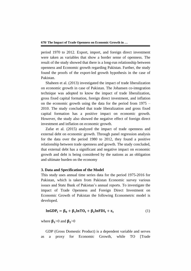
After taking into consideration the importance of the trade
openness for the promotion of economic growth of particularly,
developing nations, I decided to research the impact of trade openness
on the economic growth in case of Pakistan, therefore, rest of the
research paper is designed as follows: Section 2 will discuss the
literature review, in section 3 data and specification of the model is
described, section 4 explains the methodology, section 5 provides the
Estimation and Interpretation of Empirical Results and finally,
Conclusion and policy implications will end up the paper in section 6.
2. Literature Review
Wacziarg (2001) investigated the relationship between trade policy
and Economic Growth. He took 57 nations and used the data for the
period from 1970 to 1989. He adopted a fully specified empirical
model with the help of three trade policy variables namely, tariff
barriers and a dummy variable of liberalization, he developed an
openness index. He concluded that trade openness affects growth
mainly by raising the ratio of domestic investment to GDP and by
FDI.
Afzal (2009) investigated the impact of trade openness on
Economic Growth in the case of Pakistan, using the data over the
period 1960 – 2009. He applied the Johnson co-integration approach
and concluded that there exists a positive association among the trade
openness, financial integration, and financial growth variables.
Atif et al. (2010) investigated the impact of financial development
and trade openness on GDP growth in Pakistan using annual data over
the period 1980 – 2009. They employed the bounds testing approach
to co-integration and confirmed the validity of trade-led growth and
financial growth hypothesis in Pakistan. Aco-integration relationship
between economic growth, trade openness, and financial development
was noticed in both the long-run and short-run. Further, the analysis
showed that trade openness and financial development Granger-
Cause Economic growth in the period of study.
Muhammad et al. (2012) investigated the relationship between
openness and Economic growth in case of Pakistan using data over the
678/ The Impact of Trade Openness on Economic Growth in …
period 1970 to 2012. Export, import, and foreign direct investment
were taken as variables that show a border sense of openness. The
result of the study showed that there is a long-run relationship between
openness and Economic growth regarding Pakistan. Further, the study
found the proofs of the export-led growth hypothesis in the case of
Pakistan.
Shaheen et al. (2013) investigated the impact of trade liberalization
on economic growth in case of Pakistan. The Johansen co-integration
technique was adopted to know the impact of trade liberalization,
gross fixed capital formation, foreign direct investment, and inflation
on the economic growth using the data for the period from 1975 –
2010. The study concluded that trade liberalization and gross fixed
capital formation has a positive impact on economic growth.
However, the study also showed the negative effect of foreign direct
investment and inflation on economic growth.
Zafar et al. (2015) analyzed the impact of trade openness and
external debt on economic growth. Through panel regression analysis
for the data over the period 1980 to 2012, they found a positive
relationship between trade openness and growth. The study concluded,
that external debt has a significant and negative impact on economic
growth and debt is being considered by the nations as an obligation
and ultimate burden on the economy
3. Data and Specification of the Model
This study uses annual time series data for the period 1975-2016 for
Pakistan, which is taken from Pakistan Economic survey various
issues and State Bank of Pakistan’s annual reports. To investigate the
impact of Trade Openness and Foreign Direct Investment on
Economic Growth of Pakistan the following Econometric model is
developed.
(1)
where >0 and >0
GDP (Gross Domestic Product) is a dependent variable and serves
as a proxy for Economic Growth, while TO [Trade
Iran. Econ. Rev. Vol. 24, No. 3, 2020 /679
Openness=(X+M/GDP*100)] and FDI (Foreign Direct Investment)
are independent variables. All variables are in natural logs.
where X stands for Exports and M stands for
Imports.
is the
white noise error term, ln= natural logarithm, and t = time.
4. Methodology
We will apply both the Johnson and Autoregressive Distributed Lag
approach to co-integration. Equation (1) represents only the long-run
equilibrium relationship and may form a cointegration set provided all
the variables are integrated of order 1(1) in the case of Johansen
technique and 0 and 1, i.e. I(0) and I(1) for ARDL approach.
4.1 Unit Root Test
Almost all time - series data are found to be non-stationary and due to
this issue, we have to face the problem of spurious regression. A time-
series which have a unit root is said to be non-stationary. Therefore, to
conduct a meaningful statistical analysis one should assess the
stationary of the involved time series. A non-stationary time series yt
that is stationary in the first difference is said to be integrated of order
one and is denoted byyt I(1). In general, if a non-stationary series
must be differenced d times before becoming stationary the series is
said to be integrated of order d and is denoted by I(d). If the series is
stationary at level e.g. yt (non-differenced) it is denoted byyt I(0)
(Brooks, 2014).To test the time series data for stationary a common
method is to apply an Augmented Dickey-Fuller test (ADF) (Dickey
& Fuller, 1979) to test for a unit root. Keeping in view the error term
which is found to be white noise, Dickey and Fuller made some
modifications in their test procedure and introduced an augmented
version of the test, to overcome the problem of autocorrelation in the
test equation by including the extra lagged terms of the dependent
variable hence, this test is now known as ADF test. We, therefore,
apply the ADF test to test the unit root in time series data. The ADF
test examines the null hypothesis that a series is non-stationary by
calculating a t-statistic for δ = 0 in the following regression.

680/ The Impact of Trade Openness on Economic Growth in …
∑
where and are the deterministic elements, Yt is a variable at time
t, and is the disturbance term.
4.2 Johansen Approach to cointegration
Johansen (1988) and Johansen and Juselius (1990) have been
introduced a new co-integration technique for the long run and short-
run correlations for the multivariate equation. They proposed 4 steps
for reliable results which are as follows.
1- In the first step, we have to test the order of integration of all
variables.
2- In the second step, we should set the appropriate lag length of
the model.
3- Selection of the appropriate model keeping in view the
deterministic components in the multivariate system.
4- In the final step, the researcher should determine the rank of Пor
the number of cointegrating vectors. We use the eigenvalue
statistics and trace statistics in step four (4) to find out the
number of cointegrating equations and relationships as well as
for the values of coefficients and standard errors for the
econometric model. If we come to know that variables are
integrated of order one i.e. I(1) then, we will run the Johansen
cointegration test. Moreover, if we will also find that the
variables under study (GDP, TO and FDI) are cointegrated,
then, we will be in a position to run the VECM to examine both
the short-run as well as the long-run dynamics of the series.
The conventional ECM for cointegrated series is as follows:
∑ ∑
where Z is the ECT and is the OLS (ordinary least square) residuals
from the following long-run cointegrating regression:
and is defined as:

Iran. Econ. Rev. Vol. 24, No. 3, 2020 /681
As the coefficient of ECT measures the speed of adjustment, at
which Y returns to equilibrium after a change in X, therefore, it is,
known as the speed of adjustment.
4.3 Specifications of the ARDL Model
To empirically investigate the long-run co-integration and dynamic
interactions among the variables under consideration, we employ the
most recently introduced autoregressive distributed lag (ARDL)
approach to cointegration, developed by Pesaran et al. (2001). This
procedure is adopted for the following three reasons. Firstly, the
bounds test procedure is simple. As opposed to other multivariate
cointegration techniques such as Johanson and Juelius (1990), it
allows the cointegration relationship to be estimated by OLS once the
lag order of the model is identified. Secondly, the bounds testing
procedure does not require the pre-testing of the variables included in
the model for unit roots unlike other techniques such as the Johansen
approach. It is applicable irrespective of whether the underlying
regressors in the model are purely 1(0), 1(1), or fractionally/mutually
cointegrated. Thirdly, the test is relatively more efficient in small or
finite sample data sizes as is the case in this study. The procedure will
however crash in the presence of 1(2) series (Fosu and Magnus, 2006:
2080).
The ARDL bounds testing approach is given as follows:
∑ ∑
1
where α0 is the drift component and are white noise errors.
Based on equation (2), unres tricted error correction version of the
ARDL model is given by:
1. Note: p describes the lag of dependent variable, while q demonstrates the lag of independent variables.

682/ The Impact of Trade Openness on Economic Growth in …
∑ ∑
∑
The long-run dynamics of the model are revealed in the first part.
where the short-run effects/relationships are shown in the second part
with summation sign; while ∆ is the first difference operator; where λi
is the long-run multipliers, is the Drift, and t are white noise errors.
4.4 Bounds Testing Procedure
According to (Fosu and Magnus, 2006: 2081 )The first step in the
ARDL bounds testing approach is to estimate equation (3) by ordinary
least squares (OLS) to test for the existence of a long-run relationship
among the variables by conducting an F-test for the joint significance
of the coefficients of the lagged levels of the variables, i.e., H0: λ1 =
λ2= λ3=0 (no long-run relationship) against the alternative H1: λ1 ≠ λ2
≠λ3 ≠ 0(long-run relationship exists). We denote the test which
normalizes GDP by F GDP(GDP \TO, FDI). Two asymptotic critical
values bounds provide a cointegration test when the independent
variable is I(d) (where 0 ≤ d ≥ 1): a lower value assuming the
regressors are I(0), and an upper value assuming purely I(1)
regressors. If the F-statistic is above the upper critical value, the null
hypothesis of no long-run relationship can be rejected irrespective of
the order of integration for the time series. Conversely, if the test
statistic falls below the lower critical value the null hypothesis cannot
be rejected. Finally, if the statistic falls between the lower and upper
critical values, the result is inconclusive. The approximate critical
values for the F and t-tests were obtained from Pesaran et al. (2001).
In the next step, once cointegration is estimated, the conditional
ARDL (p, q1, q2) long-run model derives from the following equation:
∑ ∑ 1
∑
1. Note: In ARDL approach, the log of TO is not taken.

Iran. Econ. Rev. Vol. 24, No. 3, 2020 /683
where all variables under consideration have already been explained
and defined. We use the Akaike information criteria (AIC) to select
the order of the ARDL (p, q1, q2,) model in the three variables. In the
third and final step, to get the short-run dynamic parameters we
estimate the error correction model. We specify it as under:
∑ ∑
∑
Here α, β, are the short-run dynamic coefficients of the
model’s convergence to equilibrium and 𝜼 is the speed of adjustment,
where ECM is the error correction term and is defined as:
∑ ∑
∑
4.5 Granger Causality Test
To ascertain the direction of causation between the series, we use the
Granger Causality test proposed by Granger (1969, 1988). The
Granger Causality equations are specified as follows:
∑ ∑
∑ ∑
where it is assumed that both and are uncorrelated white noise
error terms.
684/ The Impact of Trade Openness on Economic Growth in …
∑ ∑
Then trade openness (TO) does not Granger cause Economic
Growth /(GDP) in equation (7), and Economic growth (GDP) does not
Granger cause Trade Openness (TO) in equation (8). It then follows
that Trade Openness (TO) and (GDP) / Economic growth are
independent, otherwise both series could be interpreted as a cause to
each other.
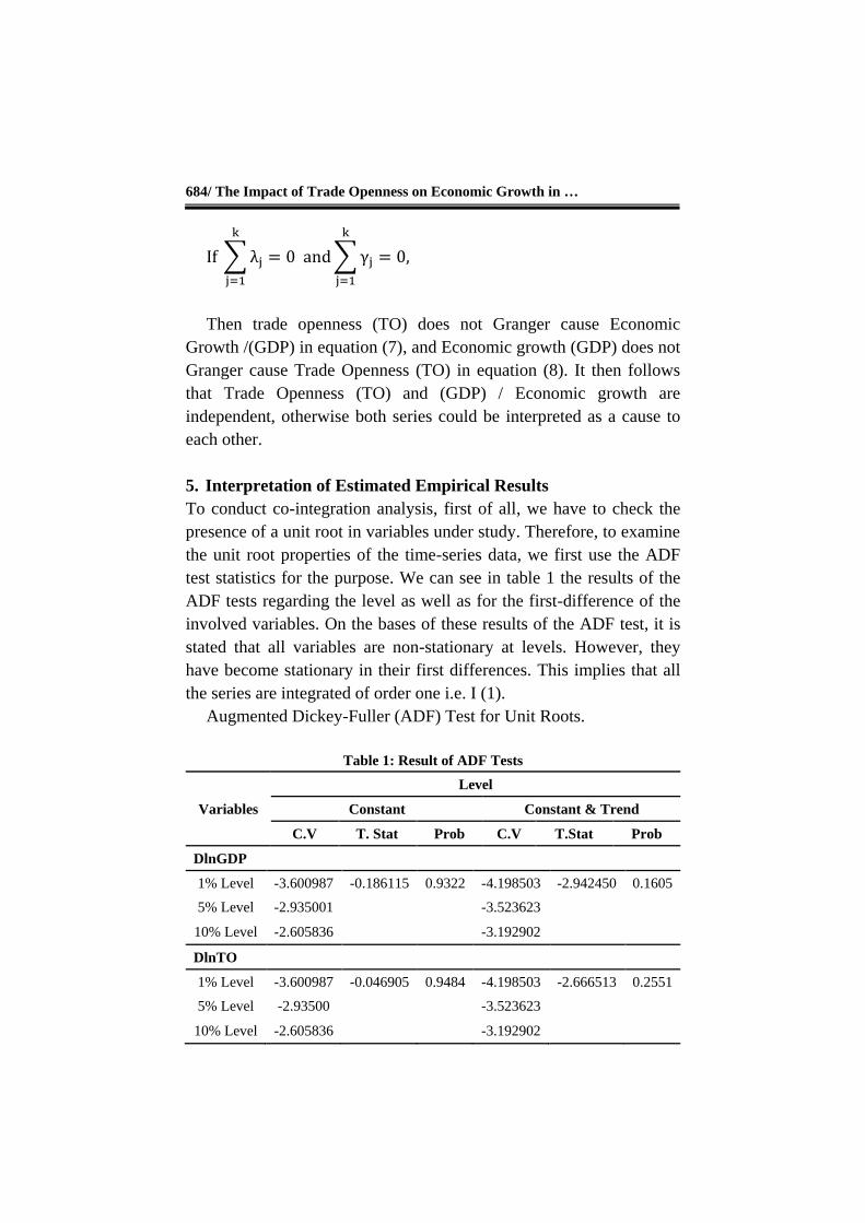
5. Interpretation of Estimated Empirical Results
To conduct co-integration analysis, first of all, we have to check the
presence of a unit root in variables under study. Therefore, to examine
the unit root properties of the time-series data, we first use the ADF
test statistics for the purpose. We can see in table 1 the results of the
ADF tests regarding the level as well as for the first-difference of the
involved variables. On the bases of these results of the ADF test, it is
stated that all variables are non-stationary at levels. However, they
have become stationary in their first differences. This implies that all
the series are integrated of order one i.e. I (1).
Augmented Dickey-Fuller (ADF) Test for Unit Roots.
Table 1: Result of ADF Tests
Variables
Level
Constant Constant & Trend
C.V T. Stat Prob C.V T.Stat Prob
DlnGDP
1% Level -3.600987 -0.186115 0.9322 -4.198503 -2.942450 0.1605
5% Level -2.935001
-3.523623
10% Level -2.605836
-3.192902
DlnTO
1% Level -3.600987 -0.046905 0.9484 -4.198503 -2.666513 0.2551
5% Level -2.93500
-3.523623
10% Level -2.605836
-3.192902

Iran. Econ. Rev. Vol. 24, No. 3, 2020 /685
Variables
Level
Constant Constant & Trend
C.V T. Stat Prob C.V T.Stat Prob
DlnFDI
1% Level -3.600987 -1.768131 0.3906 -4.198503 -2.007237 0.5801
5% Level -2.935001
-3.523623
10% Level -2.605836
-3.192902
Variables
First Difference
Constant Constant & Trend
C.V T.Stat Prob C.V T.Stat Prob
DlnGDP
1% Level -3.605593 -6.316443 0.0000 -4.205004 -6.242977 0.0000
5% Level -2.936942
-3.526609
10% Level -2.606857
-3.194611
DlnTO
1% Level -3.605593 -5.226404 0.0001 -4.205004 -5.285597 0.0005
5% Level -2.936942
-3.526609
10% Level -2.606857
-3.194611
DlnFDI
1% Level -3.605593 -7.230589 0.0000 -4.205004 -7.327092 0.0000
5% Level -2.936942
-3.526609
10% Level -2.60685
-3.194611
Source: Research findings and calculations (Eviews 9).
Lag Length Selection Process
To follow the Johansen cointegration approach, we have to determine
the appropriate lag length. So in the second step, we do the selection
of appropriate lag length by using different well-known information
criteria. The results are reported in Table 2.

686/ The Impact of Trade Openness on Economic Growth in …
Table 2: VAR (Vector Regression) Lag Order Selection Criteria
Endogenous variables: D(lnGDP)
Exogenous variables: C D(lnTO) D(lnFDI)
Sample: 1975 – 2016
Included observations: 33
Lag LogL LR FPE AIC SC HQ
0 29.61994 NA 0.011670 -1.613329 -1.477283* -1.567554
1 29.70788 0.154574 0.012342 -1.558054 -1.376659 -1.497020
2 30.24906 0.918361 0.012705 -1.530246 -1.303503 -1.453954
3 30.29403 0.073590 0.013485 -1.472366 -1.200273 -1.380815
4 30.88899 0.937507 0.013854 -1.447817 -1.130376 -1.341008
5 30.95231 0.095937 0.014712 -1.391049 -1.028259 -1.268981
6 37.52814 9.564846* 0.010539* -1.728978* -1.320840 -1.591652*
7 37.56257 0.047990 0.011235 -1.670459 -1.216971 -1.517874
8 37.56295 0.000512 0.012019 -1.609876 -1.111040 -1.442033
Source: Research findings and calculations (Eviews 9).
Notes: * indicates lag order selected by the criterion
LR: sequential modified LR test statistic (each test at 5% level)
FPE: Final prediction error
AIC: Akaike information criterion
SC: Schwarz information criterion
HQ: Hannan-Quinn information criterion
Johansen’s Cointegration Analysis
Johansen’s test in table 3 reports and indicates that there exists one co-
integration relation among Economic Growth (GDP), Trade Openness
(TO), and Foreign Direct Investment (FDI). Since the trace statistic
shown in table 3 is greater than the five percent critical value (50.89>
42.91) so the null hypothesis of no cointegration is rejected. However,
we cannot reject the null hypothesis which describes that there is at
most one cointegrating vector because (23.80 < 25.87).

Iran. Econ. Rev. Vol. 24, No. 3, 2020 /687
Table 3: Unrestricted Cointegration Rank Test, Trace, and Maximum
Eigenvalue Statistics
Hypothesized No. of CE(s)
Eigen value
Trace Statistic
Max-Eigen Statistic
0.05Critical Value Trace
Statistic
0.05 Critical Value Max-
Eigen Statistic
Prob.** Trace
Statistic
Prob.** Max-Eigen
Statistic None* 0.538802 50.89038 27.08746 42.91525 25.82321 0.0066 0.0339
At most 1 0.346913 23.80292 14.91155 25.87211 19.38704 0.0885 0.1985
At most 2 0.224338 8.891364 8.891364 12.51798 12.51798 0.1871 0.1871
Source: Research findings and calculations (Eviews 9).
Notes:
There are six lags in the VAR model. Both tests indicate 1 cointegrating equation at
the 0.05 level.
*denotes rejection of the null hypothesis at the 0.05 level.
**MacKinnon-Haug-Michelis (1999) p-values.
The maximum eigenvalue test is shown in table 3 also reports the
same result and confirms the existence of the only one cointegration
relationship among the variables under study. Thus the null hypothesis
of no co-integration is once again rejected on the bases of the fact that
the maximum eigenvalue statistic is greater than 5% critical value
(27.0874 >25.8232). However, the null hypothesis, which describes
that there is at most one co-integration vector is not rejected because
(14.9115 < 19.3870).

688/ The Impact of Trade Openness on Economic Growth in …
Table 4: Cointegrating Equation / (Long–run Model)
Sample (adjusted): 1982 –2016
Included observations: 35 after adjustments
Standard errors in ( ) & t-statistics in [ ]
Cointegrating Eq CointEq1
lnGDP(-1) 1.000000
lnTO(-1) 0.695367
(0.48703)
[ 1.42777]
lnFDI(-1) 0.315998
(0.19288)
[ 1.63831]
@TREND(75) -0.127326
(0.04313)
[-2.95241]
C -13.50627
Source: Research findings and calculations (Eviews 9).
Table 5: Vector Error Correction Estimates/Model
Error Correction: D(lnGDP) D(lnTO) D(lnFDI)
CointEq1 -0.422713 0.353814 -0.598824
(0.10128) (0.18562) (0.50834)
[-4.17390] [ 1.90614] [-1.17801]
D(lnGDP(-1)) -0.264030 0.567665 1.942103
(0.21985) (0.40295) (1.10352)
[-1.20094] [ 1.40878] [ 1.75991]
D(lnGDP(-2)) -0.241968 0.314295 1.602652
(0.21609) (0.39606) (1.08465)
[-1.11974] [ 0.79356] [ 1.47757]
D(lnGDP(-3)) 0.279585 -0.008865 1.404417
(0.20672) (0.37888) (1.03760)
[ 1.35249] [-0.02340] [ 1.35353]
D(lnGDP(-4)) 0.469146 -0.613672 -1.579342
(0.21932) (0.40198) (1.10086)
[ 2.13907] [-1.52664] [-1.43465]

Iran. Econ. Rev. Vol. 24, No. 3, 2020 /689
Error Correction: D(lnGDP) D(lnTO) D(lnFDI)
D(lnGDP(-5)) 0.716970 -0.648577 0.508937
(0.23276) (0.42660) (1.16828)
[ 3.08036] [-1.52035] [ 0.43563]
D(lnGDP(-6)) 0.306130 -1.143148 -1.880475
(0.24283) (0.44505) (1.21884)
[ 1.26069] [-2.56856] [-1.54285]
D(lnTO(-1)) -0.083959 0.177501 1.476782
(0.17133) (0.31401) (0.85995)
[-0.49005] [ 0.56527] [ 1.71728]
D(lnTO(-2)) 0.135226 -0.037942 0.426647
(0.17835) (0.32688) (0.89520)
[ 0.75821] [-0.11607] [ 0.47659]
D(lnTO(-3)) 0.401112 -0.038745 1.262118
(0.17909) (0.32824) (0.89892)
[ 2.23972] [-0.11804] [ 1.40404]
D(lnTO(-4)) 0.363774 -0.737984 -1.702031
(0.18823) (0.34500) (0.94481)
[ 1.93257] [-2.13911] [-1.80145]
D(lnTO(-5)) 0.429774 -0.483400 0.262186
(0.19986) (0.36630) (1.00316)
[ 2.15040] [-1.31968] [ 0.26136]
D(lnTO(-6)) 0.541848 -1.226322 -1.673755
(0.21010) (0.38508) (1.05459)
[ 2.57894] [-3.18458] [-1.58711]
D(lnFDI(-1)) 0.130967 0.027828 0.125291
(0.05587) (0.10241) (0.28045)
[ 2.34399] [ 0.27174] [ 0.44675]
D(lnFDI(-2)) 0.129793 -0.203137 -0.157894
(0.04121) (0.07553) (0.20684)
[ 3.14969] [-2.68961] [-0.76337]
D(lnFDI(-3)) -0.032034 -0.024692 0.190488
(0.04199) (0.07696) (0.21076)
[-0.76292] [-0.32086] [ 0.90384]

690/ The Impact of Trade Openness on Economic Growth in …
Error Correction: D(lnGDP) D(lnTO) D(lnFDI)
D(lnFDI(-4)) 0.087942 -0.007741 0.166255
(0.04500) (0.08248) (0.22588)
[ 1.95424] [-0.09386] [ 0.73604]
D(lnFDI(-5)) 0.080896 0.038316 -0.200595
(0.04132) (0.07574) (0.20742)
[ 1.95762] [ 0.50590] [-0.96711]
D(lnFDI(-6)) 0.098546 0.065254 0.226771
(0.04245) (0.07780) (0.21307)
[ 2.32143] [ 0.83870] [ 1.06428]
C 0.044883 -0.037508 -0.242977
(0.06797) (0.12457) (0.34115)
[ 0.66037] [-0.30110] [-0.71224]
R-squared 0.904968 0.776757 0.732548
Adj. R-squared 0.784593 0.493982 0.393776
Sum sq. resids 0.077407 0.260023 1.950180
S.E. equation 0.071836 0.131662 0.360572
F-statistic 7.517943 2.746907 2.162364
Source: Research findings and calculations (Eviews 9).
Estimated VECM with GDP as Target Variable
GDP = -0.422 ECTt-1 – 0.264 GDPt-1-0.241 GDPt-2 + 0.279GDPt-3 +
0.469 GDPt-4 + 0.716 GDPt-5+ 0.306 GDPt-6 – 0.0839 TOt-1+ 0.1352 TOt-2
+ 0.4011 TO t -3+ 0.363 TOt-4 + 0.429TOt-5+ 0.541 TOt-6 + 0.130 FDI +t-1+
0.129 FDIt-2 – 0.032 FDIt-3+ 0.087 FDIt-4 + 0.080 FDIt-5+ 0.098 FDIt-6 +
0.0448.
Cointegrating Equation: Since the variables are cointegrated, the
estimated long-run cointegrating equation using Vector Error
Correction is presented below.
Z t-1 = ECTt-1 = yt-1-βo-β1 Xt-1 (Long-run Model)
ECTt-1 = 1.000000lnGDPt-1 + 0.695367InTOt-1 + 0.315998ln FDIt-1 –
0.127326

Iran. Econ. Rev. Vol. 24, No. 3, 2020 /691
The above long-run model estimates have been proved a positive
long-run stable correlation among the variables under study. Though
the estimated coefficient for TO is not statistically highly significant,
it is positive. The positive coefficient of TO indicates that a 1%
increase in TO will cause the GDP to increase by 0.695%. The
estimated coefficient of FDI is also positive indicating that a unit
increase in FDI will lead to a 0.315% increase in Economic Growth in
Pakistan. The results are consistent with earlier findings of (Anorou
and Ahmad 1999) investigated the relationship between trade
openness and economic growth for five Asian countries and found the
evidence of long-run cointegration between openness and economic
growth for all the nations under consideration.
Wald Test of Short-run Causality
On the bases of VECM, we have three (3) error correction models. So
out of these three, I shall choose the 1st one D(lnGDP) to perform the
Wald test, because in table 5 D(lnGDP) [D(lnGDP) = C (1)* (Error
correction model for GDP)] is my target variable. The following is my
error correction model in table 6, while GDP is the dependent
variable. As C(1)* is the coefficient of the Co-integrating model
/equation and from this cointegrating equation, I am taking the
residuals and after taking those residuals that will be error correction
term so, that is under C(1)* coefficient1.
1. C(1)* = C(1)*( lnGDP(-1) + 0.695366710747*LNTO(-1) +0.315997889218*lnFDI(-1) - 0.127326436528*@TREND(75) -13.506274853 ) see table 6. Notes: In Table 5 we can see that all three models have no p-value,so in order to know the p-value for each variable I have been used the system equation .Now, we can see the p - value of each variable and p-value of F-statistic in table 6. System equation= D(LNGDP) = C(1)*( LNGDP(-1) + 0.695366710747*LNTO(-1) + 0.315997889218*LNFDI(-1) - 0.127326436528*@TREND(75) - 13.506274853 ) + C(2)*D(LNGDP(-1)) + C(3)*D(LNTO(-1)) + C(4)*D(LNFDI(-1)) + C(5)*D(LNGDP(-2)) + C(6)*D(LNTO(-2)) + C(7)*D(LNFDI(-2)) + C(8)*D(LNGDP(-3)) + C(9)*D(LNTO(-3)) + C(10)*D(LNFDI(-3)) + C(11)*D(LNGDP(-4)) + C(12)*D(LNTO(-4)) + C(13)*D(LNFDI(-4)) + C(14)*D(LNGDP(-5)) + C(15)*D(LNTO(-5)) + C(16)*D(LNFDI(-5)) + C(17)*D(LNGDP(-6)) + C(18)*D(LNTO(-6)) + C(19)*D(LNFDI(-6)) + C(20)

692/ The Impact of Trade Openness on Economic Growth in …
Table6: Error Correction Model
Dependent Variable: D(lnGDP)
Method: Least Squares (Gauss-Newton / Marquardt steps)
Sample (adjusted): 1982 – 2016
Included observations: 35 after adjustments
D(lnGDP) = C(1)*( lnGDP(-1) + 0.695366710747*LNTO(-1) +
0.315997889218*lnFDI(-1) - 0.127326436528*@TREND(75) -
13.506274853) + C(2)*D(lnGDP(-1)) + C(3)*D(lnTO(-1)) + C(4)
*D(lnFDI(-1)) + C(5)*D(lnGDP(-2)) + C(6)*D(lnTO(-2)) + C(7)
*D(lnFDI(-2)) + C(8)*D(lnGDP(-3)) + C(9)*D(lnTO(-3)) + C(10)
*D(lnFDI(-3)) + C(11)*D(lnGDP(-4)) + C(12)*D(lnTO(-4)) +
C(13)*D(lnFDI(-4)) + C(14)*D(lnGDP(-5)) + C(15)*D(lnTO(-5)) +
C(16)*D(lnFDI(-5)) + C(17)*D(lnGDP(-6)) + C(18)*D(lnTO(-6)) +
C(19)*D(lnFDI(-6)) + C(20)]
Coefficient Std. Error t-Statistic Prob.
C(1) -0.422713 0.101275 -4.173898 0.0008
C(2) -0.264030 0.219853 -1.200938 0.2484
C(3) -0.083959 0.171327 -0.490049 0.6312
C(4) 0.130967 0.055874 2.343989 0.0333
C(5) -0.241968 0.216093 -1.119738 0.2804
C(6) 0.135226 0.178350 0.758207 0.4601
C(7) 0.129793 0.041208 3.149688 0.0066
C(8) 0.279585 0.206719 1.352491 0.1963
C(9) 0.401112 0.179091 2.239716 0.0407
C(10) -0.032034 0.041989 -0.762919 0.4573
C(11) 0.469146 0.219322 2.139068 0.0493
C(12) 0.363774 0.188233 1.932572 0.0724
C(13) 0.087942 0.045001 1.954235 0.0696
C(14) 0.716970 0.232755 3.080355 0.0076
C(15) 0.429774 0.199857 2.150403 0.0482
C(16) 0.080896 0.041323 1.957620 0.0691
C(17) 0.306130 0.242827 1.260694 0.2267
C(18) 0.541848 0.210105 2.578944 0.0210
C(19) 0.098546 0.042451 2.321433 0.0348
C(20) 0.044883 0.067966 0.660370 0.5190
R-squared 0.904968
Adj R-squared 0.784593
F-statistic 7.517943
Prob (F-Statistic) 0.000129
Source: Research Findings and calculations (Eviews 9).

Iran. Econ. Rev. Vol. 24, No. 3, 2020 /693
C(1) -0.422 is the residual of the one-period lag residual of the
cointegrating vector among the GDP, TO, FDI. The C(1) - 0.422 is
negative and it is also highly significant because P-value (0.0008) is
less than a 5% level of significance. It means that TO and FDI have a
long-run causality on GDP.
Short Run Causality
To check the short-run causality from TO and FDI to GDP, I shall use
the chi-square value of Wald statistics. We know, that the coefficient
from C(3) to C(18) are the coefficients of Trade openness. We,
therefore, first Check that whether or not the coefficients [C(3) to
C(18) for TO] and [C(4) to C(19) for FDI] jointly influence the GDP.
From Table 7, It is concluded that the chi-square probability is less
than a 5% level of significance on the bases of which I reject the Null
hypothesis and conclude that there is a short-run causality from TO
and FDI to GDP.
Table 7: Short-run Causality between Trade Openness (TO) and GDP
Short Run Causality between Trade Openness (TO) and (GDP)
Wald Test:
Test Statistic Value Df Probability
F-statistic 2.669760 (6, 15) 0.0575
Chi-square 16.01856 6 0.0137
Null Hypothesis: C(3)=C(6)=C(9)=C(12)=C(15)=C(18)=0
Null Hypothesis Summary:
Normalized Restriction (= 0) Value Std. Err.
C(3) -0.083959 0.171327
C(6) 0.135226 0.178350
C(9) 0.401112 0.179091
C(12) 0.363774 0.188233
C(15) 0.429774 0.199857
C(18) 0.541848 0.210105

694/ The Impact of Trade Openness on Economic Growth in …
Short-run Causality between Foreign Direct Investment (FDI) and GDP
Wald Test:
Test Statistic Value Df Probability
F-statistic 4.490569 (6, 15) 0.0085
Chi-square 26.94342 6 0.0001
Null Hypothesis: C(4)=C(7)=C(10)=C(13)=C(16)=C(19)=0
Null Hypothesis Summary:
Normalized Restriction (= 0) Value Std. Err.
C(4) 0.130967 0.055874
C(7) 0.129793 0.041208
C(10) -0.032034 0.041989
C(13) 0.087942 0.045001
C(16) 0.080896 0.041323
C(19) 0.098546 0.042451
Source: Research findings and calculations (Eviews 9).
Estimated Result Based on ARDL (6, 6, 5) Model
Where the ARDL model approach allows us to proceed, irrespective
of whether the underlying regressors are I(1), I(0), or fractionally
integrated, it also imposes some restrictions that the series must not be
integrated of order two i.e., I(2). Therefore, to confirm that variables
are not integrated of order two, we have already been used the
Augmented Dickey-Fuller test (See Table 1) with maximum lag and
found that all the variables are integrated of order one i.e. 1(1). Then,
since neither of our series is 1(2) we can now apply the
Autoregressive Distributed Lag (ARDL) bounds testing approach to
estimate the impact of TO and FDI on the Economic growth of
Pakistan.
Furthermore, before the adoption of (ARDL) bounds test to co-
integration, we have been selected the appropriate lag length by using
Akaike information criteria [(AIC=-2(1/T)+2(K/T) ].
Iran. Econ. Rev. Vol. 24, No. 3, 2020 /695
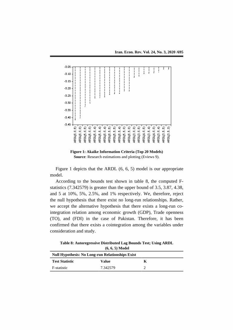
Figure 1: Akaike Information Criteria (Top 20 Models)
Source: Research estimations and plotting (Eviews 9).
Figure 1 depicts that the ARDL (6, 6, 5) model is our appropriate
model.
According to the bounds test shown in table 8, the computed F-
statistics (7.342579) is greater than the upper bound of 3.5, 3.87, 4.38,
and 5 at 10%, 5%, 2.5%, and 1% respectively. We, therefore, reject
the null hypothesis that there exist no long-run relationships. Rather,
we accept the alternative hypothesis that there exists a long-run co-
integration relation among economic growth (GDP), Trade openness
(TO), and (FDI) in the case of Pakistan. Therefore, it has been
confirmed that there exists a cointegration among the variables under
consideration and study.
Table 8: Autoregressive Distributed Lag Bounds Test; Using ARDL
(6, 6, 5) Model
Null Hypothesis: No Long-run Relationships Exist
Test Statistic Value K
F-statistic 7.342579 2
696/ The Impact of Trade Openness on Economic Growth in …
Critical Value Bounds
AwqSignificance Lower Bound Upper Bound
10% 2.63 3.35
5% 3.1 3.87
2.5% 3.55 4.38
1% 4.13 5
Source: Research findings and calculations (Eviews 9).
Table 9 reveals that the estimated long-run coefficients of the
selected ARDL (6, 6, 5) model are significant at a 5% level of
significance possessing expected signs.
The coefficient of trade openness (TO) is positive and significant at
a 5% level of significance, thus supporting the contention that trade
openness (TO) carries a perceptible influence on the economic growth
in Pakistan. The positive coefficient of TO of 0.368 indicates that in
long run a unit increase in trade openness will lead to a 37 percent
increase in economic growth/GDP, all things being the same.
Moreover, the coefficient of foreign direct investment is also positive
and highly significant at a five percent level of significance
demonstrating that in the long-run, a unit increase in FDI will bring an
increase of 168 percent in the economic growth of Pakistan. Our
results are consistent with those of Afzal(2009), Darrat (1999), Jawaid
(2014), Piazolo (1995), Shabbir 2006), Shaheen and Kauser (2013),
Siddiqui 2005) and Wacziarg (2001) They found a positive
relationship between trade openness and economic growth.
Table 9: Estimated Long-run Coefficients; Using ARDL (6, 6, 5) Model
Dependent Variable: ln GDP
Variable Coefficient Std. Error t-Statistic Prob.
TO 0.368803 0.145732 2.530697 0.0223
LnFDI 1.682512 0.161301 10.430873 0.0000
C 7.865287 0.703995 11.172369 0.0000
Source: Research findings and calculations (Eviews 9).
The short-run dynamics coefficients of the estimated ARDL (6, 6,
5) model are being shown in table 10, where the lag is selected by
Akaike information criteria.

Iran. Econ. Rev. Vol. 24, No. 3, 2020 /697
Ttable10 shows that the estimated lagged error correction term
ECM(-1)/ECt-1, is -0.135943 which is highly significant at 5% level of
significance and negative (ranges between zero and one) as was
expected having probability value less than 5%, level of significance
which is 0.0000. These results support the short-run relationship / co-
integration among the variables represented by Equation 1. The
feedback coefficient is -0.135943, which suggests that
approximately13.5% disequilibrium from the previous year’s shocks
in Equation 5 converge back to the long-run equilibrium and is
corrected in the current year.
Table10: Error Correction Estimation for Estimated ARDL (6, 6, 5) Model
Dependent Variable: lnGDP
Selected Model: ARDL(6, 6, 5)
Sample: 1975– 2016
Included observations: 36
Cointegrating Form
Variable Coefficient Std. Error t-Statistic Prob.
D(lnGDP(-1)) -0.549173 0.210313 -2.611224 0.0189
D(lnGDP(-2)) -1.088791 0.164353 -6.624726 0.0000
D(lnGDP(-3)) -0.730450 0.244326 -2.989647 0.0087
D(lnGDP(-4)) -0.485372 0.130549 -3.717920 0.0019
D(lnGDP(-5)) -0.263182 0.138361 -1.902138 0.0753
D(TO) -0.155489 0.021593 -7.200909 0.0000
D(TO(-1)) -0.101315 0.051451 -1.969149 0.0665
D(TO(-2)) -0.201054 0.039633 -5.072948 0.0001
D(TO(-3)) -0.129927 0.050685 -2.563409 0.0208
D(TO(-4)) -0.115068 0.028741 -4.003613 0.0010
D(TO(-5)) -0.076906 0.033061 -2.326207 0.0335
D(lnFDI) 0.076901 0.017156 4.482423 0.0004
D(lnFDI(-1)) -0.171859 0.030695 -5.599011 0.0000
D(lnFDI(-2)) -0.122338 0.032862 -3.722772 0.0019
D(lnFDI(-3)) -0.129707 0.027575 -4.703883 0.0002
D(lnFDI(-4)) -0.062381 0.025305 -2.465150 0.0254
ECM (-1) -0.135943 0.023019 -5.905697 0.0000
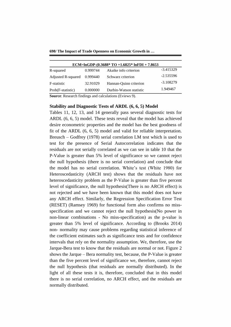
698/ The Impact of Trade Openness on Economic Growth in …
ECM=lnGDP-(0.3688* TO +1.6825* lnFDI + 7.8653
R-squared 0.999744 Akaike info criterion -3.415329
Adjusted R-squared 0.999440 Schwarz criterion -2.535596
F-statistic 32.91029 Hannan-Quinn criterion -3.108279
Prob(F-statistic) 0.000000 Durbin-Watson statistic 1.949467
Source: Research findings and calculations (Eviews 9).
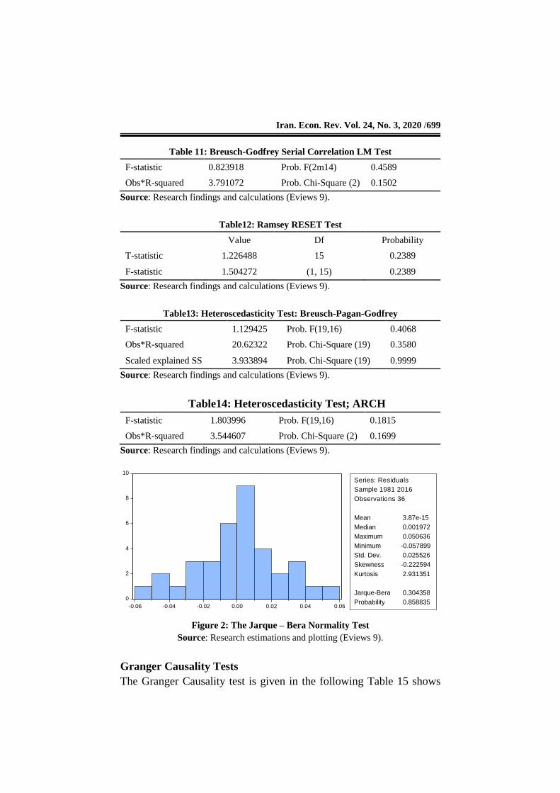
Stability and Diagnostic Tests of ARDL (6, 6, 5) Model
Tables 11, 12, 13, and 14 generally pass several diagnostic tests for
ARDL (6, 6, 5) model. These tests reveal that the model has achieved
desire econometric properties and the model has the best goodness of
fit of the ARDL (6, 6, 5) model and valid for reliable interpretation.
Breusch – Godfrey (1978) serial correlation LM test which is used to
test for the presence of Serial Autocorrelation indicates that the
residuals are not serially correlated as we can see in table 10 that the
P-Value is greater than 5% level of significance so we cannot reject
the null hypothesis (there is no serial correlation) and conclude that
the model has no serial correlation. White’s test (White 1980) for
Heteroscedasticity (ARCH test) shows that the residuals have not
heteroscedasticity problem as the P-Value is greater than five percent
level of significance, the null hypothesis(There is no ARCH effect) is
not rejected and we have been known that this model does not have
any ARCH effect. Similarly, the Regression Specification Error Test
(RESET) (Ramsey 1969) for functional form also confirms no miss-
specification and we cannot reject the null hypothesis(No power in
non-linear combinations - No miss-specification) as the p-value is
greater than 5% level of significance. According to (Brooks 2014)
non- normality may cause problems regarding statistical inference of
the coefficient estimates such as significance tests and for confidence
intervals that rely on the normality assumption. We, therefore, use the
Jarque-Bera test to know that the residuals are normal or not. Figure 2
shows the Jarque – Bera normality test, because, the P-Value is greater
than the five percent level of significance we, therefore, cannot reject
the null hypothesis (that residuals are normally distributed). In the
light of all these tests it is, therefore, concluded that in this model
there is no serial correlation, no ARCH effect, and the residuals are
normally distributed.
Iran. Econ. Rev. Vol. 24, No. 3, 2020 /699
Table 11: Breusch-Godfrey Serial Correlation LM Test
F-statistic 0.823918 Prob. F(2m14) 0.4589
Obs*R-squared 3.791072 Prob. Chi-Square (2) 0.1502
Source: Research findings and calculations (Eviews 9).
Table12: Ramsey RESET Test
Value Df Probability
T-statistic 1.226488 15 0.2389
F-statistic 1.504272 (1, 15) 0.2389
Source: Research findings and calculations (Eviews 9).
Table13: Heteroscedasticity Test: Breusch-Pagan-Godfrey
F-statistic 1.129425 Prob. F(19,16) 0.4068
Obs*R-squared 20.62322 Prob. Chi-Square (19) 0.3580
Scaled explained SS 3.933894 Prob. Chi-Square (19) 0.9999
Source: Research findings and calculations (Eviews 9).
Table14: Heteroscedasticity Test; ARCH
F-statistic 1.803996 Prob. F(19,16) 0.1815
Obs*R-squared 3.544607 Prob. Chi-Square (2) 0.1699
Source: Research findings and calculations (Eviews 9).
Figure 2: The Jarque – Bera Normality Test
Source: Research estimations and plotting (Eviews 9).
Granger Causality Tests
The Granger Causality test is given in the following Table 15 shows
0
2
4
6
8
10
-0.06 -0.04 -0.02 0.00 0.02 0.04 0.06
S e r i e s : R e s i d u a l s
S a m p l e 1 9 8 1 2 0 1 6
O b s e r v a t i o n s 3 6
Mean 3.87e-15 Median 0.001972 Maximum 0.050636 Minimum -0.057899 Std. Dev. 0.025526 Skewness -0.222594 Kurtosis 2.931351
Jarque-Bera 0.304358 Probability 0.858835
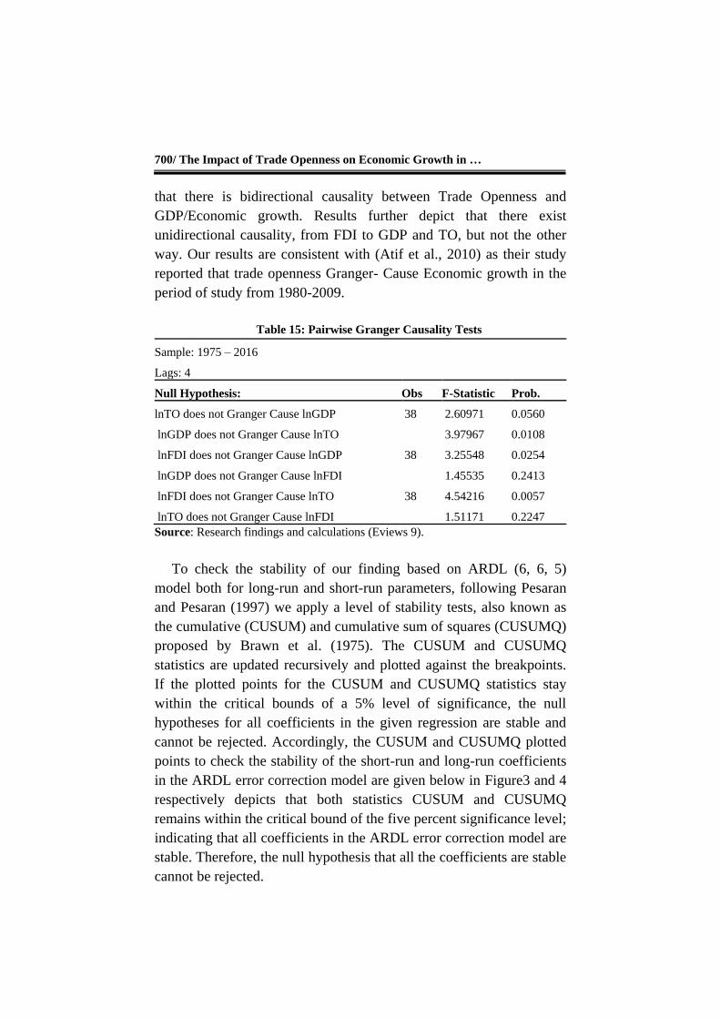
700/ The Impact of Trade Openness on Economic Growth in …
that there is bidirectional causality between Trade Openness and
GDP/Economic growth. Results further depict that there exist
unidirectional causality, from FDI to GDP and TO, but not the other
way. Our results are consistent with (Atif et al., 2010) as their study
reported that trade openness Granger- Cause Economic growth in the
period of study from 1980-2009.
Table 15: Pairwise Granger Causality Tests
Sample: 1975 – 2016
Lags: 4
Null Hypothesis: Obs F-Statistic Prob.
lnTO does not Granger Cause lnGDP 38 2.60971 0.0560
lnGDP does not Granger Cause lnTO 3.97967 0.0108
lnFDI does not Granger Cause lnGDP 38 3.25548 0.0254
lnGDP does not Granger Cause lnFDI 1.45535 0.2413
lnFDI does not Granger Cause lnTO 38 4.54216 0.0057
lnTO does not Granger Cause lnFDI 1.51171 0.2247
Source: Research findings and calculations (Eviews 9).
To check the stability of our finding based on ARDL (6, 6, 5)
model both for long-run and short-run parameters, following Pesaran
and Pesaran (1997) we apply a level of stability tests, also known as
the cumulative (CUSUM) and cumulative sum of squares (CUSUMQ)
proposed by Brawn et al. (1975). The CUSUM and CUSUMQ
statistics are updated recursively and plotted against the breakpoints.
If the plotted points for the CUSUM and CUSUMQ statistics stay
within the critical bounds of a 5% level of significance, the null
hypotheses for all coefficients in the given regression are stable and
cannot be rejected. Accordingly, the CUSUM and CUSUMQ plotted
points to check the stability of the short-run and long-run coefficients
in the ARDL error correction model are given below in Figure3 and 4
respectively depicts that both statistics CUSUM and CUSUMQ
remains within the critical bound of the five percent significance level;
indicating that all coefficients in the ARDL error correction model are
stable. Therefore, the null hypothesis that all the coefficients are stable
cannot be rejected.

Iran. Econ. Rev. Vol. 24, No. 3, 2020 /701
-12
-8
-4
0
4
8
12
01 02 03 04 05 06 07 08 09 10 11 12 13 14 15 16
CUSUM 5% Significance Figure 3: Plot of Cumulative Sum of Recursive Residuals
-0.4
0.0
0.4
0.8
1.2
1.6
01 02 03 04 05 06 07 08 09 10 11 12 13 14 15 16
CUSUM of Squares 5% Significance Figure 4: Plot of Cumulative Sum of Squares of Recursive Residuals
6. Conclusion and Policy Implications
The main objective of this study was the investigation of the impact of
the trade openness on economic growth in Pakistan. This study has

702/ The Impact of Trade Openness on Economic Growth in …
been empirically examined the impact of trade openness on the
economic growth of Pakistan using annual time series data for the
period 1975 – 2016. We have been employed both the Johensen and
Autoregressive Distributed Lag (ARDL) approach to cointegration.
The empirical estimated results are the sound evidence that there
exists a short-run and long-run positive and stable cointegration
among the variables. Our empirical findings further depict that trade
openness and foreign direct investment has a significant positive
impact on economic growth in Pakistan. Moreover, the Granger
causality test also confirms the bidirectional causality between trade
openness and economic growth. It is, therefore, concluded that trade
openness can play a key role as the economic growth of Pakistan is
concerned.
This study has some important policy implications, the government
should take some appropriate measures that are proved conducive to
enhance international trade, through which we can get a comparative
advantage. The following steps are suggested which the government
must adopt.
1- The government should support entrepreneurship
2- The government should make and ensure the optimal use of
natural resources.
3- Trade development authority of Pakistan must also undertake
various export promotion activities through trade exhibitions to
enhance the trade.
4- The government should do a regional trade agreement and
strategic trade policy framework.
5- The government should ensure the diversification of products
and markets. 6- Pakistan should move towards higher value-
added in exports and must establish export-processing zones.
References
Afzal, M. (2009). Impact of Trade Liberalization on Economic
Growth of Pakistan. Pakistan Development Review, 7, 68-79.
Anorou, E., & Ahmad, Y. (1999). Openness and Economic Growth:
Evidence from Selected Asian Countries. Indian Economic Journal,
47(3), 110-117.

Iran. Econ. Rev. Vol. 24, No. 3, 2020 /703
Atif, R. M., Jadoon, A., Zaman, K., Ismail, A., & Seemab, R.
(2010).Trade Liberalization, Financial Development, and Economic
Growth: Evidence from Pakistan (1980-2009). Journal of
International Academic Research, 10(2), 30-37.
Brooks, C. (2014). Introductory Econometrics for Finance. New
York: Cambridge University Press.
Darrat, A. F. (1999). Are Financial Deepening and Economic Growth
Causality Related? Another Look at the Evidence. International
Economic Journal, 13(3), 19-35.
Dickey, D. A., & Fuller, W. A. (1979). Distribution of the Estimators
for Autoregressive Time Series with a Unit Root. Journal of the
American Statistical Association, 74(366a), 427- 431.
Fosu, O. E., & Magnus, F. J. (2006). Bounds Testing Approach to
Cointegration: An Examination of Foreign Direct Investment, Trade,
and Growth Relationships. American Journal of Applied Sciences,
3(11), 2079-2085.
Godfrey, L. G. (1978). Testing Against General Autoregressive and
Moving Average Error Models when the Regressors Include Lagged
Dependent Variables. Econometrica: Journal of the Econometric
Society, 46(6), 1293-1301.
Gorgi, E., & Alipourian, M. (2008). Trade Openness and Economic
Growth in Iran, and Some OPEC Nations. Iranian Economic Review,
13(22), 31-40.
Granger, C. W. J. (1988). Some Recent Developments in the Concept
of Causality. Journal of Econometrics, 39, 199- 211.
Jawaid, S. T. (2014). Trade Openness and Economic Growth A
Lesson from Pakistan. Foreign Trade Review, 49(2), 193 -212.
Johansen, S. (1988). Statistical Analysis of Cointegration Vectors.
Journal of Economic Dynamics and Control, 12(6), 231 - 254.

704/ The Impact of Trade Openness on Economic Growth in …
Johansen, S., & Juselius, K. (1990). Maximum likelihood Estimation
and Inference on Cointegration with Applications to the Demand for
Money. Oxford Bulletin of Economics, 52(2), 169 -210.
Muhammad, S. D., Hussain, A., & Ali, S. (2012). The Causal
Relationship between Openness and Economic Growth: Empirical
Evidence in the Case of Pakistan. Pakistan Journal of Commerce and
Social Sciences (PJCSS), 6(2), 382- 391.
Pesaran, H. M., & Pesaran, B. (1997). Working with Microfit 4.0: An
Introduction to Econometrics. London: Oxford University Press.
Pesaran, M. H., Shin, Y., & Smith, R. J. (2001). Bounds Testing
Approach to the Analysis of Level Relationships. Journal of Applied
Econometrics, 16(3), 289 -326.
Ramsey, J. B. (1969). Tests for Specification Errors in Classical
Linear Least-Squares Regression Analysis. Journal of the Royal
Statistical Society, Series B (Methodological), 350- 371.
Shabbir, A. N. (2006). Trade Openness and Economic Growth.
Pakistan Economic and Social Review, XLIV(1), 137-154.
Shaheen, S., & Kauser, M. M. (2013). Impact of Trade Liberalization
on Economic Growth in Pakistan. Interdisciplinary Journal of
Contemporary Research in Business, 5(5), 228 -240.
Siddiqui, A. H. (2005). Impact of Trade Openness on Output Growth
for Pakistan: An Empirical Investigation. The Journal of Market
Forces, 1(1), 3 -10.
Wacziarg, R. (2001). Measuring the Dynamic Gains from Trade.
World Bank Economic Review, 15(3), 393-429.
White, H. (1980). A Heteroscedasticity-consistent Covariance Matrix
Estimator and a Direct Test for Heteroscedasticity. Econometrica:
Journal of the Econometric Society, 48(4), 817- 838.

Iran. Econ. Rev. Vol. 24, No. 3, 2020 /705
Yanikkaya, H. (2003). Trade Openness and Economic Growth: A
Cross-country Empirical Investigation. Journal of Development
Economics, 72(1), 57- 89.
Zafar, M., Sabri, P. S. U., Ilyas, M., & Kousar, S. (2015). The Impact
of Trade Openness and External Debt on Economic Growth: New
Evidence from South Asia; East Asia and the Middle East. Science
International, 27(1), 509- 516.