
The Impact of Thermal Imaging Camera Display Quality on Fire
154
NIST GCR 09-926 The Impact of Thermal Imaging Camera Display Quality on Fire Fighter Task Performance Justin Lawrence Rowe Department of Fire Protection Engineering University of Maryland College Park, MD 20742
Transcript of The Impact of Thermal Imaging Camera Display Quality on Fire

NIST GCR 09-926
The Impact of Thermal Imaging Camera Display Quality on Fire
Fighter Task Performance
Justin Lawrence Rowe Department of Fire Protection Engineering
University of Maryland College Park, MD 20742


NIST GCR 09-926
The Impact of Thermal Imaging Camera Display Quality on Fire
Fighter Task Performance
Prepared for U.S. Department of Commerce
Building and Fire Research Laboratory National Institute of Standards and Technology
Gaithersburg, MD 20899-8661
By Justin Lawrence Rowe
Department of Fire Protection Engineering University of Maryland
College Park, MD 20742
June 2009
U.S. Department of Commerce
Gary Locke, Secretary
National Institute of Standards and Technology Patrick D. Gallagher, Deputy Director

Notice
This report was prepared for the Building and Fire Research Laboratory of the National Institute of Standards and Technology under Grant number 70NANB7H6005. The statement and conclusions contained in this report are those of the authors and do not necessarily reflect the views of the National Institute of Standards and Technology or the Building and Fire Research Laboratory.

ABSTRACT
Title of Document: THE IMPACT OF THERMAL IMAGING
CAMERA DISPLAY QUALITY ON FIRE
FIGHTER TASK PERFORMANCE
Justin Lawrence Rowe, Master of Science, 2008
Directed By: Associate Professor Dr. Frederick W. Mowrer,
Department of Fire Protection Engineering
Thermal imaging cameras (TIC) have become a vital fire fighting tool for the first
responder community but there are currently no standardized quality control
regulations. The purpose of the study was to understand the impact of TIC display
image quality on a fire fighter’s ability to perform a hazard recognition task. Test
subjects were asked to identify a fire hazard by observing infrared images. The
image matrix considered the interactions of several image characteristics including
contrast, brightness, spatial resolution, and noise. The results were used to create a
model function to predict the effect of image quality on user performance. This
model was recommended to be incorporated in image quality test methods in
development at the National Institute of Standards and Technology. These
recommendations will also be provided to the National Fire Protection Association
for use in an upcoming standard on fire fighting TIC.

THE IMPACT OF THERMAL IMAGING CAMERA DISPLAY QUALITY ON
FIRE FIGHTER TASK PERFORMANCE.
By
Justin Lawrence Rowe
Thesis submitted to the Faculty of the Graduate School of the
University of Maryland, College Park, in partial fulfillment
of the requirements for the degree of
Master of Science
2008
Advisory Committee:
Associate Professor Dr. Frederick W. Mowrer, Chair
Professor Dr. James A. Milke
Assistant Professor Dr. Peter B. Sunderland

ii
Acknowledgements
The contributions and efforts of many individuals deserve recognition for the
production of this work. I would like to thank my thesis advisor Dr. Frederick
Mowrer for his assistance on obtaining the grant to fund this project and helping me
to obtain my Master of Science degree. I would like to thank Dr. Francine Amon
from the National Institute of Standards and Technology (NIST) for bringing me onto
the thermal imaging project as an undergraduate student. She has been a mentor to
me. I am grateful for the time and energy she devoted to this project and her help
with the completion of this paper. I would also like to thank Dennis Leber of NIST
for his assistance particularly on the statistics portion of this work. A great deal of
time was spent meeting with Francine and Dennis over the past year and this project
would not have taken shape the way it did without them. I would also like to thank
others from NIST including Jay McElroy and Roy McLane for their help with the
construction work and fellow researchers Josh Dinaburg, Aykut Yilmaz, Andrew
Lock and Jed Kurry who were around to discuss and help with any issues. I would
like to thank Army’s Night Vision Laboratories, in particular, John Hixson and Jim
Thomas for allowing NIST to use their perception laboratory and for their support
with data collection. I would also like to thank Kelly Campbell and Alexandra Ford
for their graphic design assistance, and Jennifer Davis for her editorial reviews.
Finally, I would like to thank the members of my thesis committee, Dr. James Milke
and Dr. Peter Sunderland, and the Fire Protection Engineering Program at the
University of Maryland for their help in furthering my academic career.

iii
Table of Contents
Acknowledgements ....................................................................................................... ii
Table of Contents ......................................................................................................... iii
List of Tables ................................................................................................................ v
List of Figures .............................................................................................................. vi
Chapter 1: TIC Overview.............................................................................................. 1
1.1 Introduction to TIC for First Responders............................................................ 1
1. 2 TIC Background................................................................................................. 2
1.2.1 Basic Function ............................................................................................. 2
1.2.1.1 Infrared Optics ...................................................................................... 4
1.2.1.2 Detector Designs ................................................................................... 5
1.2.2 Applications for Fire Service ....................................................................... 8
1.3 Development of NFPA 1801 .............................................................................. 9
1.3.1 NIST Involvement ....................................................................................... 9
1.3.2 Bench-Scale Test Methods Developed by NIST ....................................... 11
1. 4 Project Goals .................................................................................................... 14
Chapter 2: Image Processing ...................................................................................... 16
2. 1 Introduction to Image Processing .................................................................... 16
2.2 Histograms ........................................................................................................ 16
2. 3 Image Quality Characteristics .......................................................................... 17
2.3.1 Contrast ...................................................................................................... 18
2.3.2 Brightness .................................................................................................. 21
2.3.3 Spatial Resolution ...................................................................................... 23
2.3.4 Nonuniformity and Noise .......................................................................... 28
2.4 Image Processing Techniques ........................................................................... 36
2.4.1. Processing in the Spatial Domain ............................................................. 36
2.4.1.1 Point Processing .................................................................................. 37
2.4.1.2 Histogram Equalization ...................................................................... 41
2.4.1.3 Convolution in the Spatial Domain..................................................... 44
2.4.2 Image Processing in Frequency Domain ................................................... 51
2.4.2.1 Fourier Transforms ............................................................................. 51
4.2.4.1.1 The 1-D Fourier Transform ......................................................... 52
4.2.4.1.2 The 2-D Fourier Transform ......................................................... 55
2.4.2.2 Spatial Frequency Filtering ................................................................. 58
2.4.2.2.1 Filtering Techniques .................................................................... 60
Chapter 3: Human Perception Experimental Design .................................................. 69
3.1 Approach ........................................................................................................... 69
3.2 Night Vision Laboratory (NVL) ....................................................................... 70
3.3 Image Production .............................................................................................. 71
3.3.1 Hazards ...................................................................................................... 71
3.3.2 Scene .......................................................................................................... 74
3.3.3 Image Capturing......................................................................................... 77
3.4 Defining the Scenario Criteria .......................................................................... 78
3.4.1 Robustness Factors..................................................................................... 78
iv
3.4.2 Primary Factors .......................................................................................... 80
3.5 Defining the Image Set ..................................................................................... 82
3.5.1 Restrictions ................................................................................................ 82
3.5.2 Pristine Image Set ...................................................................................... 82
3.5.3 Primary Factor Design Points .................................................................... 83
3.5.4 Calculations................................................................................................ 85
3.5.4.1 Contrast and Brightness ...................................................................... 85
3.5.4.2 Spatial Resolution ............................................................................... 85
3.5.4.3 Noise and Nonuniformity ................................................................... 88
3.6 Image Processing .............................................................................................. 89
Chapter 4: Modeling Human Perception .................................................................... 94
4.1 Objective ........................................................................................................... 94
4.2 Test Subjects ..................................................................................................... 94
4.3 Experiment ........................................................................................................ 95
4. 4 Data .................................................................................................................. 96
4. 5 Logistic Regression Model .............................................................................. 97
4.6 Cross Validation................................................................................................ 98
4.7 Model Deviance and Partial Deviance ............................................................ 103
4.8 Informal Goodness of Fit Test ........................................................................ 104
4.9 Chi-Square Goodness of Fit Test .................................................................... 107
4.10 Deviance Goodness of Fit Test ..................................................................... 108
4.11 Fitted Values and Confidence Intervals ........................................................ 109
Chapter 5: Summary and Conclusions ...................................................................... 112
5.1 Summary of Model Fit .................................................................................... 112
5.2 Recommendation for Model Use in NFPA 1801 ............................................ 112
5.3 Future Work .................................................................................................... 114
Appendices ................................................................................................................ 116
Appendix A ........................................................................................................... 116
Appendix B Image Processing Program ............................................................... 121
Appendix C Test Subject Background .................................................................. 135
Appendix D Example of Design Point.................................................................. 136
Bibliography ............................................................................................................. 141

v
List of Tables
Table 1- 1TIC Applications .......................................................................................... 8
Table 3- 1 Robustness Definitions .............................................................................. 79
Table 3- 2 Primary Factor Definitions ........................................................................ 81
Table 3- 3 Design Points ............................................................................................. 84
Table 4- 1Primary Factors .......................................................................................... 97
Table 4- 2 Multiple logistic regression coefficients ................................................... 98
Table 4- 3 Informal Goodness of Fit Test with 5 Classes......................................... 105
Table 4- 4 Informal Goodness of Fit Test using 7 Classes ....................................... 106
Table 4- 5 Goodness of Fit Test ................................................................................ 108

vi
List of Figures
Figure 1- 1 Transmissivity of common combustion products as a function of
wavelength for a one meter pathlength (Grosshandler 1993) ....................................... 3
Figure 1- 2 Spatial Resolution Source Target, NFPA 1801-F09-ROP ....................... 12
Figure 2- 1 IR image of an office work station ........................................................... 17
Figure 2- 2 Image histogram of Figure 2- 1 ................................................................ 18
Figure 2- 3 Image with low contrast ........................................................................... 19
Figure 2- 4 Image histogram of Figure 2- 3. ............................................................... 19
Figure 2- 5 Image of office with high brightness ....................................................... 21
Figure 2- 6 Histogram of Figure 2- 5 .......................................................................... 22
Figure 2- 7 Image with low brightness ....................................................................... 22
Figure 2- 8 Histogram of Figure 2- 7 .......................................................................... 23
Figure 2- 9 MTF for a generic imaging system .......................................................... 25
Figure 2- 10 Generic MTFA ....................................................................................... 27
Figure 2- 11 Generic Comparison of MTF curves...................................................... 28
Figure 2- 12 Probability Distribution Histogram of Uniform Noise .......................... 30
Figure 2- 13 Probability Distribution Histogram of Gaussian Distributed Noise ...... 31
Figure 2- 14 Probability Distribution Histogram of Salt and Pepper Noise ............... 33
Figure 2- 15 Image degraded by Gaussian distributed noise ...................................... 33
Figure 2- 16 Image histogram ..................................................................................... 34
Figure 2- 17 Image degraded by salt and pepper noise .............................................. 35
Figure 2- 18 Image histogram ..................................................................................... 35
Figure 2- 19 Linear Mapping ...................................................................................... 38
Figure 2- 20 Image degraded using point processing ................................................. 39
Figure 2- 21 Image Histogram .................................................................................... 40
Figure 2- 22 Point processing using nonlinear transfer functions .............................. 41
Figure 2- 23 Original Image ....................................................................................... 43
Figure 2- 24 Image histogram of Figure 2- 23 ............................................................ 43
Figure 2- 25 Image after histogram equalization ........................................................ 43
Figure 2- 26 Image histogram after equalization ........................................................ 44
Figure 2- 27 Schematic of kernel operations .............................................................. 45
Figure 2- 28 Neighborhood averaging kernel ............................................................. 47
Figure 2- 29 Image corrupt with noise ........................................................................ 48
Figure 2- 30 Image processed using associated kernel shown in Figure 2- 31........... 49
Figure 2- 31 Gaussian kernel ...................................................................................... 49
Figure 2- 32 Image processing used associated kernel shown in Figure 2- 33........... 49
Figure 2- 33 Gaussian Kernel ..................................................................................... 50
Figure 2- 34 Image processing used Gaussian kernel shown in Figure 2- 35 ............ 50
Figure 2- 35 Gaussian Kernel ..................................................................................... 50
Figure 2- 36 Image of a circle ..................................................................................... 56
Figure 2- 37 Frequency Magnitude Spectrum of Figure 2- 36 ................................... 57
Figure 2- 38 Image of square ...................................................................................... 57
Figure 2- 39 Frequency Magnitude Spectrum of Figure 2- 38 ................................... 57
Figure 2- 40 Flow chart of frequency filtering of images ........................................... 59
Figure 2- 41 One-dimensional low pass filter............................................................. 61
Figure 2- 42 Two-dimensional low pass filter ............................................................ 61

vii
Figure 2- 43 Example of ringing artifacts ................................................................... 62
Figure 2- 44 Butterworth filter curves with varying cutoff frequencies ..................... 64
Figure 2- 45 Butterworth filter curves with varying function orders.......................... 64
Figure 2- 46 Magnitude spectrum of 2-D Butterworth filter ...................................... 65
Figure 2- 47 Original Image ....................................................................................... 65
Figure 2- 48 Image modified using Butterworth filter ................................................ 66
Figure 2- 49 High Pass 2-D Butterworth filter ........................................................... 67
Figure 2- 50 Image processed with high pass Butterworth filter ................................ 67
Figure 3- 1 Overheated electrical outlets .................................................................... 71
Figure 3- 2 Crushed wire under table leg .................................................................... 72
Figure 3- 3 Buried hotspot in chair ............................................................................. 72
Figure 3- 4 Living room scene .................................................................................... 75
Figure 3- 5 Living room scene .................................................................................... 76
Figure 3- 6 Office scene .............................................................................................. 76
Figure 3- 7 Office scene .............................................................................................. 77
Figure 3- 8 Hazard location divisions ......................................................................... 79
Figure 3- 9 Thermal clutter ......................................................................................... 80
Figure 3- 10 Flowchart of image processing .............................................................. 92
Figure 4- 1 Average response for design points ......................................................... 96
Figure 4- 2 Formation of modeling and validating datasets ....................................... 99
Figure 4- 3 Main effects only.................................................................................... 100
Figure 4- 4 Main effects + all two term interactions ................................................ 100
Figure 4- 5 Main effects + all two term interactions - contrast/spatial resolution
interaction ................................................................................................................. 101
Figure 4- 6 Main effects +all two term interactions ................................................. 101
Figure 4- 7 Average deviation from observed values ............................................... 102
Figure 4- 8 Diagnostic plot of estimated proportions with 5 classes ........................ 105
Figure 4- 9 Diagnostic plot of estimated proportions using 7 classes ...................... 106

1
Chapter 1: TIC Overview
1.1 Introduction to TIC for First Responders
Thermal imaging cameras (TIC)1 are becoming an integral tool to the first responder
community, particularly firefighters, law enforcement officers, and hazardous material
personnel, by enhancing visibility in operating conditions such as harsh structural fire
scenarios and in situations where the only indication of a material is surface temperature
and/or differences in emissivity (e.g. hazardous gas or liquid materials). In particular,
fire fighters applying TIC for search and rescue, structural navigation, hose stream
directing, locating hot spots during overhaul, and fire size-up operations among others.
TIC are improving first responder’s ability to effectively perform their jobs by decreasing
response time in hazardous situations and thus improving safety and reducing overall fire
losses.
Currently, there are no standards or performance regulations TIC for fire fighting, as
there are for other first responder equipment such as clothing, helmets, SCBA apparatus,
and PASS devices. Adoption of standardized TIC performance testing methods will
benefit first responders by providing objective test results to compare the different
camera models and technologies for deciding the most cost effective purchase while still
providing adequate performance. Standardized test methods also provide a way for TIC
manufacturers to evaluate existing cameras and drive the development of newer
technologies to create better fire fighting tools.
1 TIC is used as an acronym for both the singular and plural forms of thermal imaging camera(s),
whichever form is applicable to the context of the sentence.

2
1. 2 TIC Background
1.2.1 Basic Function
Handheld TIC take advantage of infrared (IR) radiative heat transfer by focusing the net
radiation from an object whether emitted or reflected onto the thermal detector array
inducing an increase in material temperature which triggers a proportional signal output.
Radiation is transmitted through the atmosphere in the form of electromagnetic waves at
specific frequencies. The intensity of the radiation at each frequency is a function of the
temperature and surface properties. As the temperature of an object increases, the
wavelength of peak intensity decreases as described by Planck’s formula in Equation1-1
(Theory of Thermography 2007).
( )
2
5 /
2
1b hc kT
hcW
eλ λ
π
λ=
− 1-1
where Wλb is the blackbody spectral radiant emittance at wavelength λ, c is 3 x 10⁸ m/s
(speed of light), h is 6.6 x 10⁻³⁴
, k is 1.4 x 10⁻²³
(Boltzmann’s constant), T is the absolute
temperature (K) of a blackbody, and λ is the wavelength (µm).
By integrating Planck’s formula in Equation 1-1 over all frequencies, the total radiant
emittance of a blackbody becomes the Stefan-Boltzmann Law shown in Equation1-2.
4
bW Tσ= 1-2
Real objects almost never act as a perfect blackbody over an extended range of
wavelengths and therefore the emissivity of a surface is used to describe the ratio of the
spectral radiant power from the object to that from a blackbody at the same temperature
and wavelength (Theory of Thermography 2007). The radiant emittance of real world

objects is shown in the modified S
account for the emissivity of a surface.
where ε is the emissivity.
TIC detect radiation in the IR
there is a high transmittance of
for the fire service are tailored to
range, IR waves are less susceptible to
particulates in the atmosphere
Figure 1- 1 Transmissivity of common combustion products as a functi
for a one meter pathlength (Grosshandler 1993)
3
shown in the modified Stefan-Boltzmann Law shown in Equation
account for the emissivity of a surface.
4W Tεσ=
is the emissivity.
tect radiation in the IR spectral band of the electromagnetic spectrum because
there is a high transmittance of IR waves through fire related atmosphere
for the fire service are tailored to focus on the 8-14 µm wavelengths because within this
IR waves are less susceptible to diffraction or scattering from water
particulates in the atmosphere as shown in Figure 1- 1.
Transmissivity of common combustion products as a function of wavelength
for a one meter pathlength (Grosshandler 1993)
shown in Equation 1-3 to
1-3
spectral band of the electromagnetic spectrum because
atmospheres. TIC designed
because within this
water vapor or
on of wavelength

4
IR waves transmit extremely well through carbon monoxide, carbon dioxide and water
and relatively well through smoke. The transmittance at the near visible band, less than 1
µm, is almost completely blocked by smoke which illustrates the ineffectiveness of the
human eye and other visual optical systems in smoky combustion environments and
emphasizes the need for TIC in the fire service.
Incident radiative transfer onto the detector array is not the only important form of heat
transfer. The radiative heat lost from the detector pixels to the surroundings acts to cool
the detector pixel, increasing the response time of the TIC. Heat loss also occurs through
conduction. Each detector pixel is attached to a substrate by supporting legs. Heat is lost
through conduction from the detector pixel down the supporting leg to the substrate. In
some detector designs such as the hybrid layout discussed in more detail in the following
sections, conduction also occurs when heat transfers from one detector pixel to a
neighboring pixel. This process, known as thermal spreading, is critical to avoid when
designing thermal arrays because it affects the resolution [Kruse 1997].
1.2.1.1 Infrared Optics
TIC for the fire service are designed with IR optics to focus the radiation onto an array of
thermal detectors. The IR optics are similar to that of any optical system except for the
materials used for the lens and optic focal lengths. A standard transparent lens transmits
electromagnetic waves in the visual spectrum but not at the IR wavelengths so TIC use
materials that transmit well in the 8-14 µm wavelengths, such as Zinc Selenide and
Germanium. The optics of TIC also have a wide field of view (FOV) and a far focusing

5
distance. Fire fighters need the ability to see a wide FOV to survey a scene more rapidly.
Typically, TIC for the fire service are designed with a FOV between 40-60º. The
focusing distance ranges from 1 m out to infinity with no manual focusing options. The
FOV and minimum 1 m focal length makes the TIC hard to perform testing in a bench
scale lab because large targets and ample space are required to fill the FOV of the
camera’s with thermal targets and measuring equipment. Finally, the optics are designed
to avoid narcissus and glare. Narcissus occurs when there is a reflection in the optic
components in which the detectors see themselves (Holst 1998). Coatings are applied to
the optics to avoid internal reflections.
1.2.1.2 Detector Designs
The development of uncooled IR imaging arrays in the 1980’s offered a substantial
advantage over cooled IR detectors in that they did not have be cryogenically cooled.
TIC could therefore be produced at low cost and designed to be lightweight to be used for
countless applications for the military and civilian sectors, including fire fighting.
Handheld TIC utilize IR arrays that operate using thermal detectors because they do not
require cooling systems and large power supplies (Dinaburg 2007).
Thermal IR detectors utilize a sensitive material that has some measureable property that
changes dramatically with temperature. The most common detection mechanisms used
for handheld TIC are the resistive microbolometer and pyroelectric detectors (Holst
2000). The microbolometer detectors utilize a material with a temperature-dependent
resistance to measure a change in resistance of each detector pixel due to the absorption
of the IR radiation (Kruse 1997). The two most common materials used in
6
microbolometers are vanadium oxide (VOx) and amorphous silicon. Both of these
materials have high temperature coefficients of resistance (TCR), one of the most
important properties in determining the voltage response of a detector because the TCR is
directly proportional to the voltage response (Muralt 2001).
Pyroelectric detectors utilize the ability of certain materials to change in polarization due
to a change in temperature or otherwise known as the pyroelectric effect. When a
material is heated (or cooled) positive and negative charges migrate to opposite faces of
the sensor creating polarization. The change in surface charge is measured during the
transient temperature change resulting from the incoming radiation. Because pyroelectric
detectors measure transient temperature changes, they require a chopper to continuously
reference the temperature of each pixel to ambient. The detectors are usually made from
materials that have very low thermal mass so the temperature change is rapid (Tsai and
Young 2003). The most common material used in TIC is a ferroelectric material called
barium strontium titanate (BST). Ferroelectic materials offer an additional advantage
because with the application of an external electric field, the pyroelectric coefficient is
increased. The pyroelectric coefficient is directly proportional to the change in charge of
the material. This phenomenon is known as the field-enhanced pyroelectric effect
(Muralt 2001).
In either type of detector design, the detector array is attached to a readout integration
circuit (ROIC) which functions to read in and format the detector’s signal output. Due to
the sensitivity of the thermal detector’s response to small temperature changes and the
heat transfer physics, thermal isolation is critical to the quality of the TIC. Because of the

7
importance of thermal isolation the primary methods for attaching the thermal detector
array to the ROIC will be discussed.
The support structure provides three main functions; mechanical support, and a thermal
and electrically conducting path. One of the most important aspects of the design of the
supporting structure is to minimize the thermal conductance of the supporting legs that
are attached to the detector pixels to increase response time. The detector pixels must
also be thermally isolated to avoid thermal spreading. The two main approaches for
providing the support are the monolithic and hybrid design. In the hybrid approach the
detector pixel layer is separated from a silicon substrate layer which typically
incorporates the ROIC. The two layers are joined by a bump bond at two supporting legs
which provides the mechanical support as well as the high electrical conduction and low
thermal conduction. The monolithic approach is to have the sensor and electronic
elements on the same layer.
There are advantages and disadvantages to both types of support structures. The
monolithic design sacrifices image quality for a relatively lower cost to manufacture than
the hybrid design. Because the detector pixel, supporting structure, and read-out
electronics are on the same layer, the detector pixels must be placed farther away from
each other. The layout is beneficial to minimize thermal spreading because the substrate
acts as a heat sink. However, this also produces a poor fill factor. The two layer hybrid
design typically use a laser scribed technique to separate the detector pixels creating a
better fill factor and image quality but at a greater cost to manufacturer.

8
1.2.2 Applications for Fire Service
A workshop entitled “Thermal Imaging Research Needs for First Responders” was
hosted by Amon et al. to gain input from the first responder community as well as TIC
manufacturers and other stakeholders on how TIC are being used in the field. The
knowledge gained from this workshop and other TIC manufacturing literature on TIC
applications is listed in Table 1- 1 [Amon 2005].
Table 1- 1 TIC Applications
First Responder Applications for Thermal Imaging Cameras
Application Description
Search and Rescue Locate heat sources, such as victims or fallen fire fighters.
Hazard Assessment Locate and assess the severity of a fire. A TIC can be used
to find hot spots and a potential threat to adjoining
structures.
Building Assessment Analyze the integrity of a structure by identifying hazards
such as holes in the floor, hanging wires, and the failure of
load bearing structural elements.
Navigation Doors, windows, and other escape points can be located for
quick egress. TIC can distinguish furniture and other objects
that could block a path.
Fire Attack
Directing hose streams
Identify potential flashover or back draft conditions. Find
ventilation locations, direct hose streams, analyze the
effectiveness of the hose stream and access the severity of
the upper layer temperature.
Over-haul Quickly scan for remaining hot spots and embers that lead to
rekindling. Over-haul can be carried out more rapidly and
with minimal damage to the structure.
Wild land Fires TIC can be used on the ground or in the air to locate hot
spots in vegetation and root systems. Useful for determining
fire fighting strategies and identifying animals, people, and
nearby buildings that may be in danger.
Incident
Control/Command
Fire fighter activity can be monitored by sending images
from TIC back to the incident commander. The images can
be used to account for fire fighters, as well as make
decisions as to the tactics used to extinguish the fire. This
application can be particularly helpful in high-rise building
fires where fire fighter coordination is more difficult.
Hazardous Materials Help identify the level of liquid in hazardous material

9
containers and track the movement of hazardous material
after spillages. Fire fighters can make more accurate
decisions as to where barriers may need to be positioned,
how much hazardous material has been spilled, and the
potential risks to the nearby area.
Post-incident
Investigation
Identify the source of a fire and how the fire spreads. A TIC
can capture images of a scene while a fire is occurring. The
images can later be used as evidence for understanding and
verifying the progress of the fire situation.
The applications listed in Table 1- 1 demonstrate the exposure of TIC to a variety of
thermal targets and operating temperatures. As more fire departments are equipped with
TIC and the technologies become more advance, additional ways to utilize a TIC will be
discovered. The knowledge gained from the BFRL workshop was incorporated into the
design of the images used in this study to represent a typical TIC operating environment.
1.3 Development of NFPA 1801
1.3.1 NIST Involvement
The National Fire Protection Association (NFPA) Technical Committee of Electronic
Safety Equipment is developing a standard to govern the design, performance, testing,
and certification requirements for TIC used by first responders. The standard is currently
being created by NIST in collaboration with committees formed by users, manufacturers,
technical experts, and the public. NIST provides unbiased science-based research and
experience in fire testing including the evaluation of fire fighter personal protective
equipment. The suggestions made about the content of the standard provided by NIST
will be taken into consideration by the NFPA for use in NFPA 1801, Standard on
Thermal Imagers for the Fire Service.

10
The research at NIST, headed by Dr. Francine Amon in the Fire Fighting Technology
Group in BFRL, is focused on TIC overall system performance requirements, specifically
the output of the display screens. The requirements specified in NFPA 1801, Section 7.1,
Thermal Imager Performance Requirements, include a range of performance testing on
ingress protection, electromagnetic emissions and immunity, resistance to vibration,
impact-acceleration resistance, corrosion resistance, viewing surface abrasion resistance,
resistance to heat and flame, product label durability, cable pullout test, and most
importantly, display image quality.
The performance test methods designed by NIST treat the TIC as a “black box” to focus
on the entire system as the TIC would be used by the fire service and not the various
components separately. The display quality is of upmost importance because it is the
primary mechanism for relaying information to the user. The display image of a TIC is
influenced by a large number of factors due to the number of components involved in
converting IR radiation into a formidable image on the display screen. There are
numerous component packages available on commercial TIC which includes a variety of
detector technologies, signal processing algorithms, gain settings, optics, electronics, and
displays. However, there are very few manual adjustments to the display image that can
be performed by the user. Typically, there is only an on/off switch and maybe one more
specialty button depending on the brand of TIC. All adjustments to focus, gain,
sensitivity and other image enhancements are all automatically done by the interior
functions of the TIC. Each manufacturer has complex (and secret) algorithms to post
process the signal output of the detector array to the image formed on the display screen.

11
Every manufacturer has different techniques to improve the quality of the image and
testing each subsystem of every camera would be cumbersome and unnecessary.
Section 7.2, Imaging Performance Requirements, of NFPA 1801 applies specifically to
the quality of the display image. The test methods designed by NIST measure various
aspects of the display image quality including contrast, overall brightness, spatial
resolution, and image nonuniformity (noise). For a more detailed description of display
measurement techniques refer to the Video Electronics Standards Association (VESA)
Flat Panel Display Measurements Standard [VESA 2001]
1.3.2 Bench-Scale Test Methods Developed by NIST
The methods described in NFPA 1801, Section 8.1.6, Spatial Resolution Procedure,
incorporate measurements of image contrast, overall brightness, and spatial resolution.
The procedures require the TIC under testing to be centered one meter (the minimum
focusing distance of a TIC) from a spatial resolution target, shown in Figure 1- 2. The
TIC is required to have a line of sight perpendicular to the target.
12
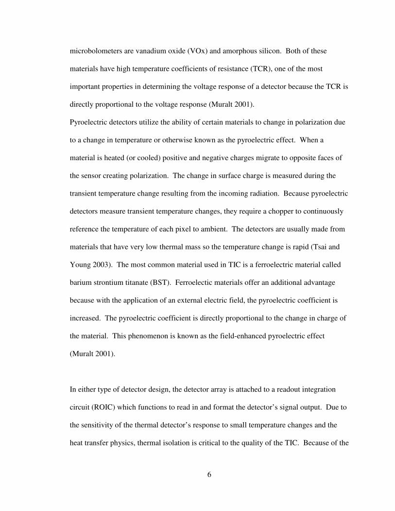
Figure 1- 2 Spatial Resolution Source Target, NFPA 1801-F09-ROP
The target design was an adaptation from a portion of the ISO 12233 test chart (ISO
12233). The target and a black backdrop are required to fill the TIC field of view (FOV).
The spatial resolution target is set to 28 C ± 0.5 C. A black shroud is placed over the
view path of the camera to block out any glare incident on display.
A calibrated luminance meter is positioned as close as possible to the TIC to capture the
FOV of the display screen. A minimum of 100 uncompressed images at a minimum 16-
bit depth are captured with the luminance meter.

13
Using the captured images, contrast, brightness, and spatial resolution calculations are
performed at each baseline index (shown in Figure 1- 2) which corresponds to a specific
spatial frequency. The contrast is calculated according to NFPA 1801 Section 8.1.6.11 at
each indexed baseline using the standard deviation of an equal amount of pixel intensities
from the heated target and backdrop. Brightness is calculated in NFPA 1801 according
to section 8.1.5.13a as the mean pixel intensity over the same region. The spatial
resolution is measured using the Modulation Transfer Function (MTF) which is
calculated using a Contrast Threshold Function (CTF) as described in the NFPA 1801
Section 8.1.6.10. The spatial resolution target utilizes essentially a square bar target to
represent spatial frequencies instead of a sinusoidal target because it is easier to
manufacturer. The CTF is defined in Equation 1-4 as
max min
max min
I ICTF
I I
−=
+ 1-4
where I is the pixel intensity at a point of interest. The CTF is defined by the ratio of the
difference between the maximum and minimum pixel intensities. The MTF and CTF can
be related mathematically through the square and sine wave relationship.
4
MTF CTFπ
= 1-5
A more detailed description of the MTF is described in Chapter 2 of this work.
The nonuniformity is calculated using the procedure described in Section 8.1.5 of NFPA
1801. The TIC is positioned near the nonuniformity target to fill the entire FOV of the
TIC. The nonuniformity target is a blackbody required to stabilize at a temperature
within 0.02 C at temperatures below 160 C and 0.05 at temperature up to 260 C. The
luminance meter is positioned again so that the TIC display fills the FOV and placed

14
under a black shroud to eliminate glare from surrounding light sources. A minimum of
100 uncompressed images are taken with the nonuniformity target at set point
temperatures of 1 C, 30 C, 100 C, 160 C, and 260 C. The standard deviation and mean
pixel intensity are calculating according NFPA 1801 Equation 8.1.5.13a and 8.1.5.13b.
The nonuniformity is defined as the ratio of the standard deviation of the pixel intensities
over the mean.
Nonuniformityσ
µ= 1-6
The maximum nonuniformity at any of the set point temperatures is deemed the
nonuniformity of the imaging system as a conservative estimate.
The calculations for contrast, brightness, spatial resolution, at each baseline index and the
maximum nonuniformity are then used as the image quality input parameters for the
logistic regression model created by the work done in this study to predict if the TIC
meets standard requirements for image quality. A complete detailed description of the
model is outlined in Chapter 4 of this work.
1. 4 Project Goals
The goal of this study was to determine the effect TIC display image quality has a fire
fighter’s ability to perform a task typically accomplished using a TIC and complement
the image quality performance test methods established at NIST by creating a model to
predict the probability of identifying a fire hazard based on the following image quality
parameters: contrast, brightness, spatial resolution, and nonuniformity (noise).

15
To accomplish the goals of this study, a perception experiment was conducted where test
subjects, who were a representative group of fire fighters that regularly use TIC, were
given a task to identify a fire hazard by observing IR images. Although there are a wide
range of tasks a fire fighter could potentially encounter and the type of images that are
displayed on the TIC could vary dramatically, hazard recognition is among the most
important TIC application and therefore was the focus of this study.

16
Chapter 2: Image Processing
2. 1 Introduction to Image Processing
Image processing includes a collection of techniques used to manipulate the visual
appearance of an image. The fundamentals needed to execute these tools to enhance or
degrade the quality of images are the focus of this chapter. Image processing can be
accomplished in both the spatial and frequency domains. Although many of the
processes are equivalent, processing in both domains will be discussed because there is
sometimes value for choosing one over the other. Color will not be included because
most TIC display images are composed of only grayscale values. In addition, color is not
accounted for in the TIC performance test methods at NIST.
2.2 Histograms
Image histograms are valuable for image processing because they display the distribution
of graylevels within an image. Histograms are essentially bar charts that show the
number of pixels of an image that have a particular pixel intensity or brightness value.
For an 8-bit image, there are 256 different possible pixel values that are usually displayed
on the x-axis of a histogram. Each pixel of an image is then placed in one of the 256
categories also known as bins. Peaks in a histogram indicate common pixel intensities
within the image while valleys show less common values. Histograms are useful for
enhancing the brightness and contrast of an image through a technique called histogram
equalization as discussed in Section 2.4.1.2 Histogram Equalization.

17
2. 3 Image Quality Characteristics
Contrast and brightness are closely related concepts because by definition they are
associated directly to the graylevel intensity value of the pixels of an image and have
common image processing techniques. It is easiest to explain these concepts visually
with images and their corresponding histograms as well as quantitatively in their
definition. For this discussion, consider an 8-bit infrared image of an office work station
shown in Figure 2- 1.
Figure 2- 1 IR image of an office work station

18
Figure 2- 2 Image histogram of Figure 2- 1
The histogram shown in Figure 2- 2 illustrates the image utilizes the full range of
graylevels of an 8-bit image from 0 to 255.
2.3.1 Contrast
The contrast of an image is the range of graylevels used to represent the scene. There are
a possible 256 shades of gray for an 8-bit imaging system. Typically, the more
graylevels an imaging system uses the higher the contrast. For a TIC, insufficient
contrast within a display image reduces the details of objects that have very similar
emitted or reflected IR radiation. In a low contrast image, more pixels in the display
image are using the same graylevel to depict different levels of radiation in a
corresponding object. Consider Figure 2- 3 and the corresponding graylevel histogram in
Figure 2- 4.

19
Figure 2- 3 Image with low contrast
Figure 2- 4 Image histogram of Figure 2- 3.
Figure 2- 3 has a lower contrast than Figure 2- 1 because fewer graylevels are being
utilized. The total number of pixels has been spread over a smaller range of graylevels.
As a result, some of the details such as the power cords and other small items on the desk
that are visible in Figure 2- 1, are indistinguishable in Figure 2- 3.

20
An image with perfect contrast is subjective and dependent on the scene the imaging
system is representing. There is no one value used to define the perfect contrast for an
image but there are several methods of quantifying the overall contrast of an image. One
method is to measure the average variation in graylevels otherwise known as the standard
deviation of graylevels [Weeks 1996]. For an N x M image, the contrast is
[ ]1 1
2
0 0
1( , )
M N
y x
contrast I x y BNM
− −
= =
= −∑ ∑ 2-1
where B is the average pixel intensity. The highest possible contrast for an 8-bit image
for example, is half the number of total graylevels or 128.
Another common method of defining contrast is
max min
max min
I Icontrast
I I
−=
+ 2-2
where the overall maximum and minimum pixel intensity of the entire image are used.
This definition of contrast is normalized from 0 to 1.
Equation 2-1 is a better definition for the contrast of an entire image than Equation 2-2.
Using Equation 2-2, two images by definition could have the same contrast but appear
very different. An 8-bit image with one pixel at a graylevel intensity of 255 and one pixel
at 0 would yield a perfect contrast of 1 even if every other pixel within the image was
128. A second image with many pixels at 0 and 255 would also yield a contrast of 1 but
a different perceived look. Equation 2-2 is a well know definition for the CTF
calculation at a specific frequency and is typically used as a measure of spatial resolution
as described in Section 1.3.2 Bench-Scale Test Methods Developed by NIST

21
2.3.2 Brightness
Brightness is the overall perceived darkness or lightness of an image. For an 8-bit image,
0 and 255 correspond to black and white and every other pixel intensity corresponds to
some shade of gray. For an N x M image I(x,y), brightness is simply defined as the
average pixel intensity within the image [Weeks 1996].
1 1
0 0
1( , )
M N
y x
brightness B I x yNM
− −
= =
= = ∑ ∑ 2-3
Compare Figure 2- 5 with an overall brightness value of 198 to the original image in
Figure 2- 1 with a brightness of 107. As the brightness increases or decreases the pixels
saturate at a 0 or 255 intensity as evident by the loss of details of the computer shown in
the lower left corner of Figure 2- 5.
Figure 2- 5 Image of office with high brightness

22
Figure 2- 6 Histogram of Figure 2- 5
Figure 2- 7 has a brightness value of 22. The image is saturated at 0 as shown in the
histogram in Figure 2- 8.
Figure 2- 7 Image with low brightness

23
Figure 2- 8 Histogram of Figure 2- 7
2.3.3 Spatial Resolution
The resolution of an imaging system is defined as the separation of two discrete targets
necessary to discern these targets on a display image. A classical method of quantifying
the spatial resolution of an imaging system is the Modulation Transfer Function (MTF).
The MTF is a measure of the ability of an imaging system to recreate the modulation of a
target to an image for a range of spatial frequencies. The overall system MTF is the
result of many subsystems such as the optics, scanners, detectors, electronics, signal
processors, and displays. MTF also applies to any one of these subsystems individual
such as display luminance value or the voltage signal of the detector array from an
infrared camera [Boreman 2001]. The NIST test methods treat the TIC as a “black box”
and focus on the evaluation of the display screen, the final product of the entire system.
Modulation is defined in Equation 2-4 as the amplitude of the pixel intensity variations
normalized by the bias level at a given frequency [Boreman 2001].

24
max min
max min
I IModulation M
I I
−= =
+ 2-4
The MTF is the ratio of modulation in the image to the object as a function of spatial
frequency described in Equation 2-5.
( )
( )( )
image
object
MMTF
M
γγ
γ= 2-5
Due to the inherent limitation in TIC system components such as the resolution of the
display and the detector cell spacing and fill factor, the reduction in the modulation of a
signal is frequency dependent. As the spatial frequency of an object increases, the
modulation depth of the image decreases and therefore the MTF decreases. Figure 2- 9
illustrates the concept of MTF for a generic imaging system.

25
Figure 2- 9 MTF for a generic imaging system
Object Intensity
Position
Image Intensity
Position
0
1
MTF
Spatial Frequency
26
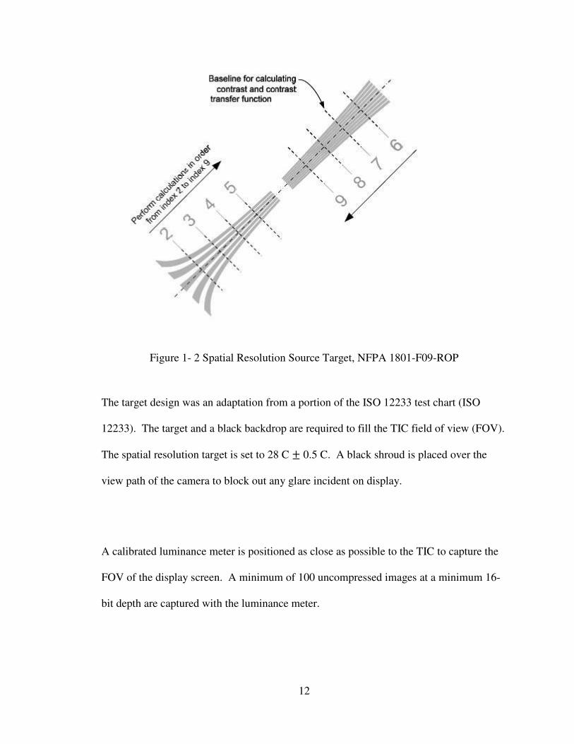
At high spatial frequencies as the MTF approaches zero, the modulation is typically no
longer due to the imaging of the target but the random modulation of random in pixel
output, known as a type of noise. The noise-equivalent modulation (NEM) characterizes
the noise in a TIC in terms of the MTF and is defined as the amount of image modulation
necessary to yield a signal to noise ratio (SNR) of unity [Boreman 2001]. This value is
also measured using the Nonuniformity calculation shown in Section 8.1.5 of NFPA 1801
[NFPA 1801 2008].
The limiting resolution of an imaging system is the location where the NEM dominates
the MTF. Any point on the MTF curve greater than the intersection of these two points is
a corrupted signal and not a testament to the resolution of the imaging system.
While the MTF provides a more complete description of image quality at all spatial
frequencies it is common to specify a single value for spatial resolution. A common
definition of the overall spatial resolution of an imaging system is integration of the MTF
curve between 0 and the spatial frequency at the intersection between the NEM and MTF
known as the MTF area (MTFA). A larger MTFA indicate better spatial resolution.
Figure 2- 10 illustrates the definition of spatial resolution.

27
Figure 2- 10 Generic MTFA
The fundamental difficulty in defining spatial resolution using the MTFA is that two
imaging systems with the same MTFA but different NEM could have a very different
performance in a particular range of spatial frequencies. Consider the two imaging
systems MTF curves in Figure 2- 11. Both imagers have the same MTFA but different
responses to spatial frequencies.

28
Figure 2- 11 Generic Comparison of MTF curves
TIC A has a higher MTF in the lower frequencies than Imager B. In the mid-range
spatial frequencies TIC B is better than TIC A
2.3.4 Nonuniformity and Noise
An undesired deviation from an ideal signal is defined as noise. Noise is typically either
a constant amplitude over all signal levels or increases with signal level resulting in more
noise in brighter areas than darker areas of an image [Smith 2007]. Noise is inherent in
all electro-optical imaging systems in all processes from the optics used to capture the
scene to the production of the display image. Detector sensors, amplifiers and cabling are
a few of the system processes sources of noise. A wide range of external factors also
influence noise, including environmental conditions, radiation, and the instability of a
light source. The most common noise that occurs in all imaging systems is detector noise
from the counting statistics of the incident photons on a detector pixel due to the discrete
nature of radiation [Russ 2002].

29
Noise is generally thought of in two main categories: uncorrelated (independent) noise
and correlated (dependent) noise. Uncorrelated noise is defined as the random graylevel
variations within an image that have no dependency on the graylevels of neighboring
pixels [Weeks 1997]. Noise is generated in images as both additive and multiplicative
noise. Our discussion is limited to uncorrelated additive noise where a recorded image
),( jiR can be defined as
( , ) ( , ) ( , )R i j T i j n i j= + 2-6
where ),( jiT is the pixel intensities of the noise free image and ),( jin is the intensity of
the noise.
Noise is generally classified by the probability distribution or the discrete histogram for
digitalized images in terms of the mean, M, and the variance σ2. The mean is defined as
max
0
G
i
i
mean M i n=
= = •∑ 2-7
where in is the probability of the noise at each graylevel i from 0 to Gmax. The variance is
defined as
max
2 2 2
0
G
i
i
i n Mσ=
= ∗ −∑ 2-8
The standard deviation can be obtained from the variance as
max
1/2
2 2
0
G
i
i
i n Mσ=
= ∗ − ∑ 2-9
A uniform distribution of noise produces random noise values with equal probability in a
range of pixel intensities.

30
1,
( )
0,
for K i JJ Kn i
otherwise
≤ ≤ −=
2-10
Figure 2- 12 displays a uniform noise histogram.
Figure 2- 12 Probability Distribution Histogram of Uniform Noise
Additive uniform noise is then the summation of the random noise value with the original
pixel value only for pixel values from KJ → .
Noise is often modeled by an additive Gaussian distributed noise because by the central
limit theorem, a large number of additive independent noise sources approaches a
Gaussian distribution [Smith 2007]. The Gaussian distribution also describes detector
noise which is one of the largest sources of noise in electro-optical imaging systems due
to the nature of radiation and the limited time and space for the detector arrays to count
the incident photons [Russ 2002].

31
Gaussian noise is expressed as
2
2
( )
2
( )2
i M
en i
σ
σ π
− −
= 2-11
and by the probability distribution histogram as
Figure 2- 13 Probability Distribution Histogram of Gaussian Distributed Noise
which has a peak at the mean. Most Gaussian distributed noise is applied to images with
a mean of 0. In other words, the highest probability of an occurrence of Gaussian noise
has a noise value of zero. The probability of the Gaussian noise decreases as the intensity
of the noise increases the farther the graylevels are from the mean. As with any statistical
Gaussian or normal distribution, 68% of the noise values lie within one standard

32
deviation, 95% within two, and 99.7% within three standard deviations. The variance
specifies the thickness of the bell shaped curve. A higher variance would create a greater
magnitude in noise intensity for more pixels.
Another common form of noise in electro-optical systems is salt-and-pepper noise where
the noise values are generally outliers that deviate far from the expected pixel intensity.
In electronic cameras, errors in data transmission generally produce saturated pixels or
white and black graylevel intensities. Salt-and-pepper noise can also occur from dust or
lint on the optics of the camera during data acquisition. Generally, salt-and-pepper noise
takes on two discrete values and occurs at a percentage of the total pixels within the
image as defined in Equation 2-12.
( )
( ) ( )
0
p pepper i J
n i p salt i K
otherwise
=
= =
2-12
The histogram of salt-and-pepper noise is
33
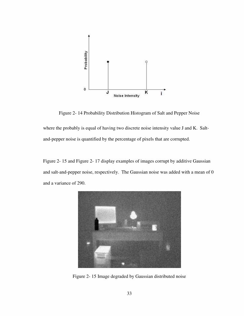
Figure 2- 14 Probability Distribution Histogram of Salt and Pepper Noise
where the probably is equal of having two discrete noise intensity value J and K. Salt-
and-pepper noise is quantified by the percentage of pixels that are corrupted.
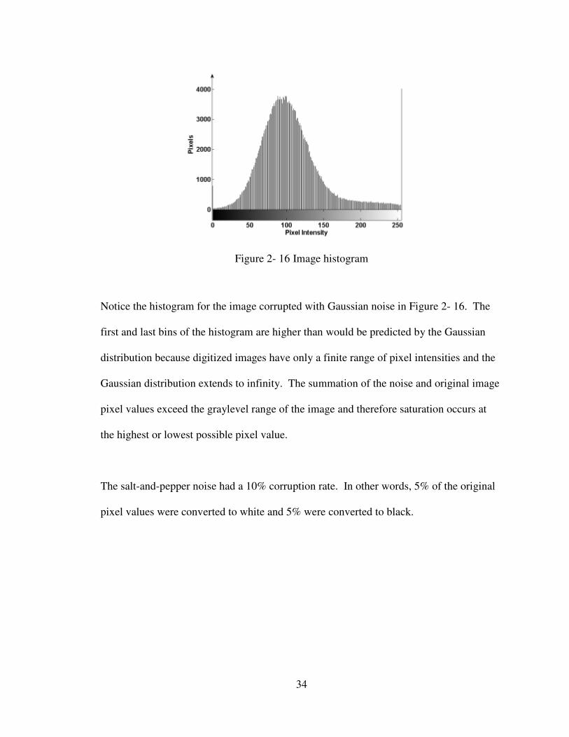
Figure 2- 15 and Figure 2- 17 display examples of images corrupt by additive Gaussian
and salt-and-pepper noise, respectively. The Gaussian noise was added with a mean of 0
and a variance of 290.
Figure 2- 15 Image degraded by Gaussian distributed noise
34
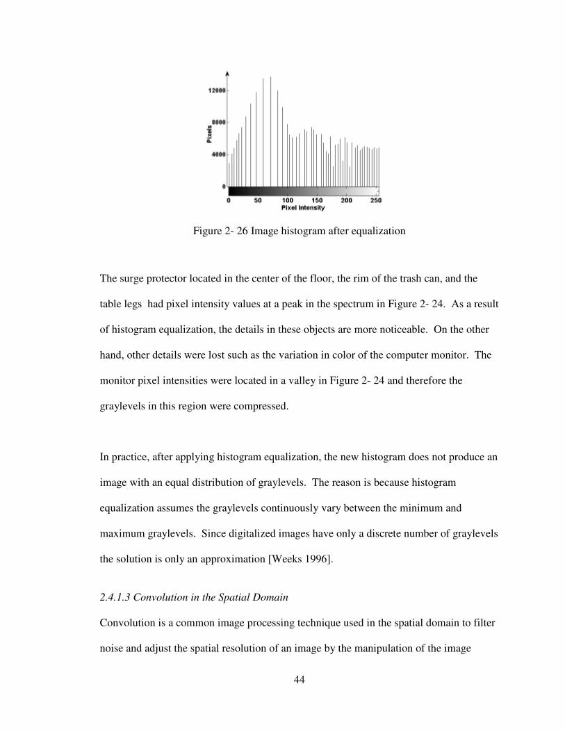
Figure 2- 16 Image histogram
Notice the histogram for the image corrupted with Gaussian noise in Figure 2- 16. The
first and last bins of the histogram are higher than would be predicted by the Gaussian
distribution because digitized images have only a finite range of pixel intensities and the
Gaussian distribution extends to infinity. The summation of the noise and original image
pixel values exceed the graylevel range of the image and therefore saturation occurs at
the highest or lowest possible pixel value.
The salt-and-pepper noise had a 10% corruption rate. In other words, 5% of the original
pixel values were converted to white and 5% were converted to black.

35
Figure 2- 17 Image degraded by salt and pepper noise
Figure 2- 18 Image histogram

36
The histogram for the salt-and-pepper noise corrupted image is as expected. The first and
last bins are higher than the original image histogram because 10% of the pixels were
converted to black and white.
The impact of noise within an image is often defined by the signal to noise ratio. For
most applications of SNR, the signal is a distinct or known value, like a DC voltage, with
respect to time. The noise is the random unwanted fluctuations in that signal. For this
discussion, the SNR is the ratio of the noise free image pixel intensities over the intensity
due to noise as function of pixel location within the image. The SNR is quantified as the
ratio of the standard deviation over all the pixels in an image such that
T
N
SNRσ
σ= 2-13
where Tσ is the standard deviation of the pixel intensities of the noise-free image and Nσ
is the standard deviation of the noise [Fisher 2003]. A high SNR would indicate that the
pixel intensities of the noise free image dominate the noise intensities causing very little
degradation to the corrupted image. In the same way, a low SNR would indicate the
noise values of the corrupted image dominate those of the original image. As the SNR
decreases the noise begins to dominate over the signal and the original image is lost.
2.4 Image Processing Techniques
2.4.1. Processing in the Spatial Domain
Processing images in the spatial domain implies modifications or operations are
performed directly to the pixel intensity values of each pixel location of the original
image. These modifications are made to each pixel value independently, known as local

37
or point processing, or these adjustments can depend on the combination or comparison
of a pixel location with its surrounding pixels, known as neighborhood processing.
Image processing in the spatial domain is less computationally demanding than
processing in the frequency domain because the images are not transformed into
frequency space and therefore advanced mathematics or processing programs are not
required. Modifications are applied directly to the image by scanning each pixel value
and performing some operation.
2.4.1.1 Point Processing
Contrast and brightness are two images characteristics that are processed in the spatial
domain by the manipulation of an image’s graylevels. Some transfer function, linear or
non-linear, is applied to the original pixel graylevel values to map these values to a new
set of graylevels.
Linear transfer functions include addition (subtraction) and multiplication (division).
Each original pixel within an image is multiplied and/or added to a constant value to
create a new pixel value. Generally, these two functions can be combined as described in
Equation 2-14.
k kP m O d= ∗ + 2-14
In Equation 2-14, m describes the slope and d describes the offset. Each original pixel,
kO is then modified by this transfer function to create a new pixel value, kP for all image
pixels, k . Figure 2- 19 illustrates the concept of linear mapping.

38
Figure 2- 19 Linear Mapping
The linear mapping of graylevels to new values is only valid within the range of the
graylevel scale which is based on the bit depth of the image. An output value exceeding
the range of the grayscale is set to the limits of that scale. For an 8-bit image, an output
value of greater than 255 would be mapped to 255 and an output value less than 0 would
be mapped to 0. The linear transfer function in Figure 2- 19 created a saturation line at
the maximum possible graylevel.
The slope of the linear transfer function in Equation 2-14 changes both the contrast and
the brightness of an image and the offset alters only the brightness. To separate the
adjustments for contrast and brightness, Equation 2-14 is rewritten as
( ) ( )k kP m O B B d= ∗ + + 2-15
where B is the average brightness of the image as defined in Equation 2-3. The variable
m changes only the contrast and the offset d changes only the brightness [Weeks 1996].

39
A slope of one and an offset of 0 in the transfer function would take each original pixel
value and map it to the same value in the modified image. If the transfer function had a
slope value greater than one than a smaller range of graylevels in the original image is
linearly spread over a larger range of graylevels in the modified image known as contrast
expansion. This is used for image enhancement to expand an image that does not utilize
the full range of graylevels available for a particular bit depth to the full range of
graylevels. This greatly improves the contrast of an image and enhances detail.
Similarly, a slope value of less than one can be used to degrade the contrast of an image.
A slope of less than one linearly decreases the amount of graylevels in the output image
that are utilized in the original image. A positive offset value would increase the overall
brightness of an image and a negative value would produce a darker image. Figure 2- 20
illustrates the use of Equation 2-15 to modify the brightness and contrast of an image
using point processing. A slope, m , value of 0.3 and an offset, d , value of 80 was used.
Figure 2- 20 Image degraded using point processing

40
Figure 2- 21 Image Histogram
Figure 2- 20 essentially has a contrast of 30% of the original image shown in Figure 2- 1
and an average overall brightness 80 graylevels higher than the original image.
Non-linear transfer functions operate in a similar fashion to linear functions with the
exception that the output pixel value will be dependent on the value of the input pixel.
Non-linear functions are typically used to enhance dark or light regions of an image that
are of interest to an observer. A non-linear transfer function can expand some portions of
grayscale range while compressing others depending on an observer’s needs. Several of
the most common types of non-linear transfer functions are the exponential and
logarithmic among others presented in Figure 2- 22.

41
Figure 2- 22 Point processing using nonlinear transfer functions
Figure 2- 22 displays the original image pixel value on the x-axis and the modified pixel
value on the y-axis after the application of a transfer function. The exponential or
squared transfer function increases the contrast of the light areas of an image while
reducing the contrast of dark areas. The logarithmic and square root transfer function
have the opposite effect. The inverse function reverses the pixel values and the identity
function leaves the image unchanged.
Transfer functions, either linear or non-linear, are an important part of image processing
because a reproducible quantitative modification can be applied to a series of images and
to create the same effect.
2.4.1.2 Histogram Equalization
Histogram equalization is used to modify the contrast and brightness of an image by
modifying the image histogram. The goal is to redistribute the graylevels of an image so

42
each graylevel has an equal probability of occurring while retaining the brightness order
of the pixels (See Figure 2- 26). In other words, the new histogram has uniformly
distributed pixel intensities but relative intensities remain in the same order as the
original image. Peaks in the histogram are spread out over a larger range of graylevels
while the valleys are compressed into fewer graylevels creating visibility in minor pixel
variations for a greater number of pixels.
For a discrete image, the process of histogram equalization can be described as
0
j
i
i
Nk
T=
=∑ 2-16
where the sum counts the total number of pixels within an image with original brightness
equal to or less than, ,j and T is the total number of pixels [Russ 2002]. For each
original brightness level, ,j the new assigned value is .k
Figure 2- 23 show an original image with its histogram as well as an image using
histogram equalization. After histogram equalization, some features in the new image
became more apparent and other details were lost.

43
Figure 2- 23 Original Image
Figure 2- 24 Image histogram of Figure 2- 23
Figure 2- 25 Image after histogram equalization
44
Figure 2- 26 Image histogram after equalization
The surge protector located in the center of the floor, the rim of the trash can, and the
table legs had pixel intensity values at a peak in the spectrum in Figure 2- 24. As a result
of histogram equalization, the details in these objects are more noticeable. On the other
hand, other details were lost such as the variation in color of the computer monitor. The
monitor pixel intensities were located in a valley in Figure 2- 24 and therefore the
graylevels in this region were compressed.
In practice, after applying histogram equalization, the new histogram does not produce an
image with an equal distribution of graylevels. The reason is because histogram
equalization assumes the graylevels continuously vary between the minimum and
maximum graylevels. Since digitalized images have only a discrete number of graylevels
the solution is only an approximation [Weeks 1996].
2.4.1.3 Convolution in the Spatial Domain
Convolution is a common image processing technique used in the spatial domain to filter
noise and adjust the spatial resolution of an image by the manipulation of the image

45
graylevels. Convolution is the replacement of a pixel value with a weighted average of
itself and the neighboring pixels using an array of integer weights known as a kernel. A
kernel is essentially a filter with an impulse response given by the kernel weights that is
applied pixel by pixel to an entire image. Each location in the kernel array corresponds
to a pixel location relative to the pixel being processed. The integer weights in the kernel
are multiplied by their corresponding pixel value and the average of these values is used
to replace the original pixel value. A kernel is typically square with odd dimensions
(3x3, 5x5, 7x7, etc.) so it can be symmetrical about a central pixel. To illustrate, consider
an original image with a pixel location ),( yxf and a 3 x 3 filter kernel ),( yxh with
weights kw .
Figure 2- 27 Schematic of kernel operations
The center of the kernel is defined by the coordinate (0, 0) and exists over the range
1,0,1, −∈yx . The new pixel value ),( yxg after convolution by ),( yxh with weights kW
can be described as

46
2 2
( 3 )
0 0
2 2
( 3 )
0 0
( 1 , 1 )
( , )
W j i
i j
W j i
i j
f x j y i h
g x y
h
+= =
+= =
− + − + ⋅
=
∑∑
∑ ∑ 2-17
The summation of the central and neighborhood pixels multiplied by the kernel weight
and then normalized by the sum of the weights produces the new pixel value.
Applying a kernel around a central pixel creates a problem at the border of an image. At
pixel location )0,0(f in Figure 2- 27, five of the nine kernel weights do not apply to any
neighboring pixel. There are several approaches to deal with this problem. The first
approach is to simply not process the edges of the images where some kernel weights
would not exist. This is not a major limitation for small kernel sizes because typically
edges do not contain the most important details of an image. A second approach is to
mirror the edge pixels as if they extended beyond the image. Finally, the kernel could
wrap around the image and take the pixel values from the opposite size of the image as if
they image was continuous. When using small kernels this problem is not a major
limitation. However, when dealing with larger kernel sizes the problem could be
significant. The convolution process would not be uniform throughout the image.
The impulse response (the values of the kernel weights) and the size of the kernel dictate
the effect of convolution on the image. The most common convolution process is a
simple neighborhood averaging kernel where the weight of each location within the
kernel is equal. This type of filter is beneficial for reducing noise by removing high

47
frequencies from an image. Figure 2- 28 illustrates a 3 x 3 kernel array for simple
neighborhood averaging.
Figure 2- 28 Neighborhood averaging kernel
The random noise pixel values are reduced because of the contribution of true image
pixel values from neighborhood pixels. In general, the larger the kernel size, the more
noise is filtered out of an image. Convolution also reduces the spatial resolution by
blurring edges and boundaries of objects in the image. In fact, convolution in the spatial
domain can be a useful tool not only for reducing noise but also for image degradation to
reduce the spatial resolution of an image.
To reduce the amount of blurring for a desired amount of noise reduction, the weight
values of the kernel can be adjusted to add a greater emphasis on the original pixel value
and the contribution of neighborhood pixels diminishes the farther away from the central
pixel. The weight values could be chosen somewhat arbitrarily depending on an
observer’s opinion when the convolution process has created a desired result. However,
it is useful to use standardized numbers for weight values so the same kernel can be
applied to multiple images for comparison.

48
The most common weighted kernel is the Gaussian kernel. This type of kernel is an
approximation of the Gaussian function along every row, column, and diagonal through
the center of the kernel [Russ 2002]. The actual numbers used in the kernel vary
particularly in the smaller kernels because discrete values are used to approximate a
smooth continuous function. The Gaussian kernel is typically described by the standard
deviation which is defined as the radius (in pixels) from the center of the filter containing
68% of the integrated magnitude of the coefficients [Russ 2002]. Consider Figure 2- 29
of an image corrupted with noise.
Figure 2- 29 Image corrupt with noise
Figure 2- 30 shows the convolution of Figure 2- 29 using several size Gaussian kernels.
Kernel size increases with standard deviation.

49
Figure 2- 30 Image processed using associated kernel shown in Figure 2- 31
Figure 2- 31 Gaussian kernel (3x3)
Figure 2- 32 Image processing used associated kernel shown in Figure 2- 33

50
Figure 2- 33 Gaussian Kernel (9 x 9)
Figure 2- 34 Image processing used Gaussian kernel shown in Figure 2- 35
Figure 2- 35 Gaussian Kernel (15 x 15)

51
As the Gaussian kernel size increases, the visibility of the noise present in the image
decreases but the sharpness of the image also decreases.
The use of neighborhood averaging kernels such as the Gaussian kernel in a convolution
process reduces the blurring effect for a given amount of noise reduction but does not
completely eliminate the reduction in spatial resolution. Neighborhood averaging kernels
operate based on the assumption that every pixel within the kernel size belongs to the
same feature in the image. Because this is not true at edges and boundaries there will
always be some reduction in the spatial resolution of an image.
To sharpen a blurry image, negative weight values can be given to a kernel for the
neighborhood pixels and a positive weight to the central pixels. The intensity of the
central pixel is magnified, sharpening edges and creating greater contrast. The process is
limited to images with small amounts of noise; otherwise, noise pixels would be
magnified and defeat the purpose of sharpening edges.
2.4.2 Image Processing in Frequency Domain
2.4.2.1 Fourier Transforms
The Fourier transform is the most common transform used for image processing in the
frequency domain because of the availability of an efficient algorithm for computing it,
known as the fast Fourier Transform [Cooley and Tukey, 1965; Bracewell, 1989].
Performing image measurements and processing operations in the frequency domain
offers some advantage over the kernel operations in the spatial domain. In many cases, it
is desired to filter out a particular spatial frequency of an image such as the removal of a
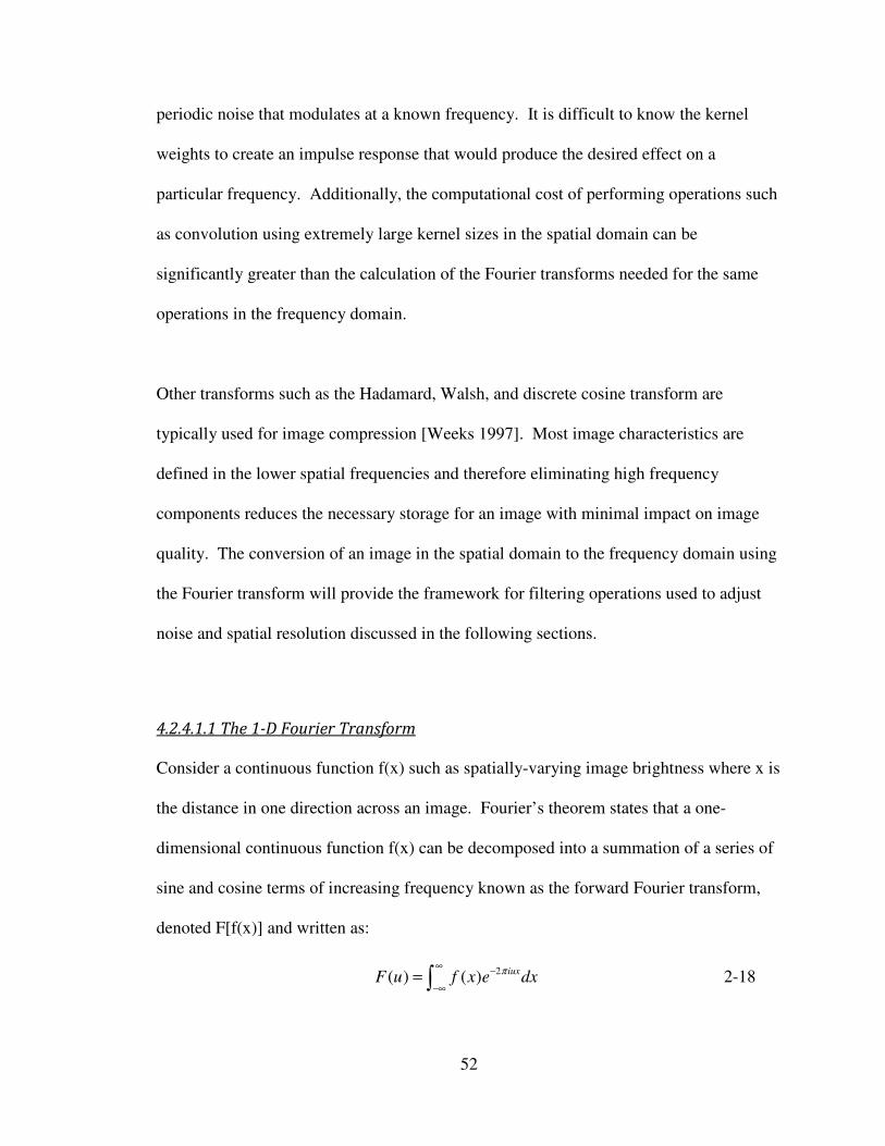
52
periodic noise that modulates at a known frequency. It is difficult to know the kernel
weights to create an impulse response that would produce the desired effect on a
particular frequency. Additionally, the computational cost of performing operations such
as convolution using extremely large kernel sizes in the spatial domain can be
significantly greater than the calculation of the Fourier transforms needed for the same
operations in the frequency domain.
Other transforms such as the Hadamard, Walsh, and discrete cosine transform are
typically used for image compression [Weeks 1997]. Most image characteristics are
defined in the lower spatial frequencies and therefore eliminating high frequency
components reduces the necessary storage for an image with minimal impact on image
quality. The conversion of an image in the spatial domain to the frequency domain using
the Fourier transform will provide the framework for filtering operations used to adjust
noise and spatial resolution discussed in the following sections.
4.2.4.1.1 The 1-D Fourier Transform
Consider a continuous function f(x) such as spatially-varying image brightness where x is
the distance in one direction across an image. Fourier’s theorem states that a one-
dimensional continuous function f(x) can be decomposed into a summation of a series of
sine and cosine terms of increasing frequency known as the forward Fourier transform,
denoted F[f(x)] and written as:
2( ) ( ) iuxF u f x e dx
π∞
−
−∞= ∫ 2-18

53
where 1−=i . Using Euler’s formula to expand Equation 2-18, the Fourier transform,
F(u), can be separated into real and imaginary components.
( ) ( ) ( )F u R u iI u= + 2-19
where )(uR is the real part of )(uF and is defined as
( ) ( ) cos(2 )R u f x ux dxπ∞
−∞
= ∫ 2-20
and )(uI is the imaginary part of )(uF
( ) ( ) sin(2 )I u f x ux dxπ∞
−∞
= − ∫ 2-21
Each sinusoidal term in the Fourier series corresponds to a spatial frequency or
specifically for this demonstration, a frequency where the brightness of the image
modulates. The Fourier frequency components can be written in terms of magnitude
otherwise known as the magnitude spectrum,
2 2( ) ( ) ( )F u R u I u= + 2-22
and phase also known as the phase spectrum,
1 ( )( ) tan
( )
I uu
R uφ −
=
2-23
The magnitude is essentially the amplitude of the brightness modulation and the phase
represents the shift in the sinusoid relative to the origin [Weeks 1996].
The Fourier Transform encodes a series of sinusoids for a range of spatial frequencies
from zero or no modulation (the average brightness of the image) to the highest spatial

54
frequency. Up until now we have considered a continuous function and the highest
spatial frequency would be dependent on the function f(x). However, digital images have
discrete brightness values at each pixel location. The integrals shown in Equations 2-20
and 2-21 are evaluated from minus to plus infinity. The discrete forward Fourier
transform for a digital image would be limited by the finite spacing of the pixels and can
be written as
1
2 /
0
1( ) ( )
Ni ux N
x
F u f x eN
π−
=
= ⋅∑ 2-24
where N depends on the number of pixels in the X-direction. The summation is
performed over terms up to one-half the dimension of the image in pixels. The final
frequency term is known as the nyquist frequency and is defined as the highest spatial
frequency that can be encoded in a digital image. The nyquist frequency is one half the
total pixels in a dimension because it requires a minimum of two pixel brightness values
to define a frequency. Because each frequency component has a real and imaginary part,
the total number of values produced by the Fourier Transform is the same as the total
number of pixels in the x-direction [Russ 2002].
One of the most important aspects of the Fourier Transform is that given )(uF , the
original spatial domain function f(x) can be recovered using the same technique.
2( ) ( ) iuxf x F u e du
π∞
−
−∞= ∫ 2-25
or in the discrete case
1
2 /
0
( ) ( )N
i ux N
u
f x F u eπ
−
=
= ⋅∑ 2-26

55
This property of Fourier transform is extremely important when using linear filtering
techniques to modification the spatial frequencies present within an image.
4.2.4.1.2 The 2-D Fourier Transform
Expanding the properties of the one-dimensional Fourier transform into two-dimensions,
entire images can be decomposed into frequency space where each pixel corresponds to a
complex value representing a magnitude and phase component. The 2-dimensional
Fourier Transform is
2 ( )1( , ) ( , ) i vx wy
F v w f x y e dxdyNM
π∞
− +
−∞
= ∫ ∫ 2-27
and its inverse as
2 ( )1( , ) ( , ) i vx wy
f x y F v w e dvdwNM
π∞
− +
−∞
= ∫ ∫ 2-28
where v and w are the frequencies in the x and y directions. For an N x M finite size
image the discrete 2-dimensional Fourier transform is
1 1
2 ( / / )
0 0
1( , ) ( , )
M Nj nx N my M
y x
F n m f x y eNM
π− −
− +
= =
= ⋅∑∑ 2-29
and its inverse as
1 1
2 ( / / )
0 0
( , ) ( , )M N
j nx N my M
m n
f x y F n m eπ
− −+
= =
= ⋅∑∑ 2-30
The terms in the Fourier series are independent of each other. Most of the image
characteristics are described in the first few terms of the series. Adding higher and higher
frequency terms improves the quality of the image, sharpening edges and providing the

56
fine details. Performing the transform at higher and higher frequencies does not alter the
previous terms.
Images in frequency space are commonly represented based on only the magnitude
values of the sinusoids called the magnitude spectrum. Sometimes the square of the
magnitude or the power is used. An image is created from the magnitude spectrum by
simply scaling the values to coincide with the graylevel range based on the bit depth of
the image (0 to 255 for an 8-bit image). The distance from the origin of the magnitude
spectrum corresponds to an increase in spatial frequency. The origin is the zero
frequency component otherwise known as the DC level (no modulation or the average
pixel intensity). The magnitude spectrum is commonly represented with the origin in the
center and increasing frequency with the radius. The orientation depends on the angle.
Figure 2- 36 and Figure 2- 38 are real images of two shapes. Figure 2- 37 and Figure 2-
39 are the representations of the corresponding magnitude spectrum.
Figure 2- 36 Image of a circle

57
Figure 2- 37 Frequency Magnitude Spectrum of Figure 2- 36
Figure 2- 38 Image of square
Figure 2- 39 Frequency Magnitude Spectrum of Figure 2- 38
Notice most of the image in frequency space is located near the origin or at the lowest
spatial frequencies. The magnitudes of the lowest frequencies are high creating bright
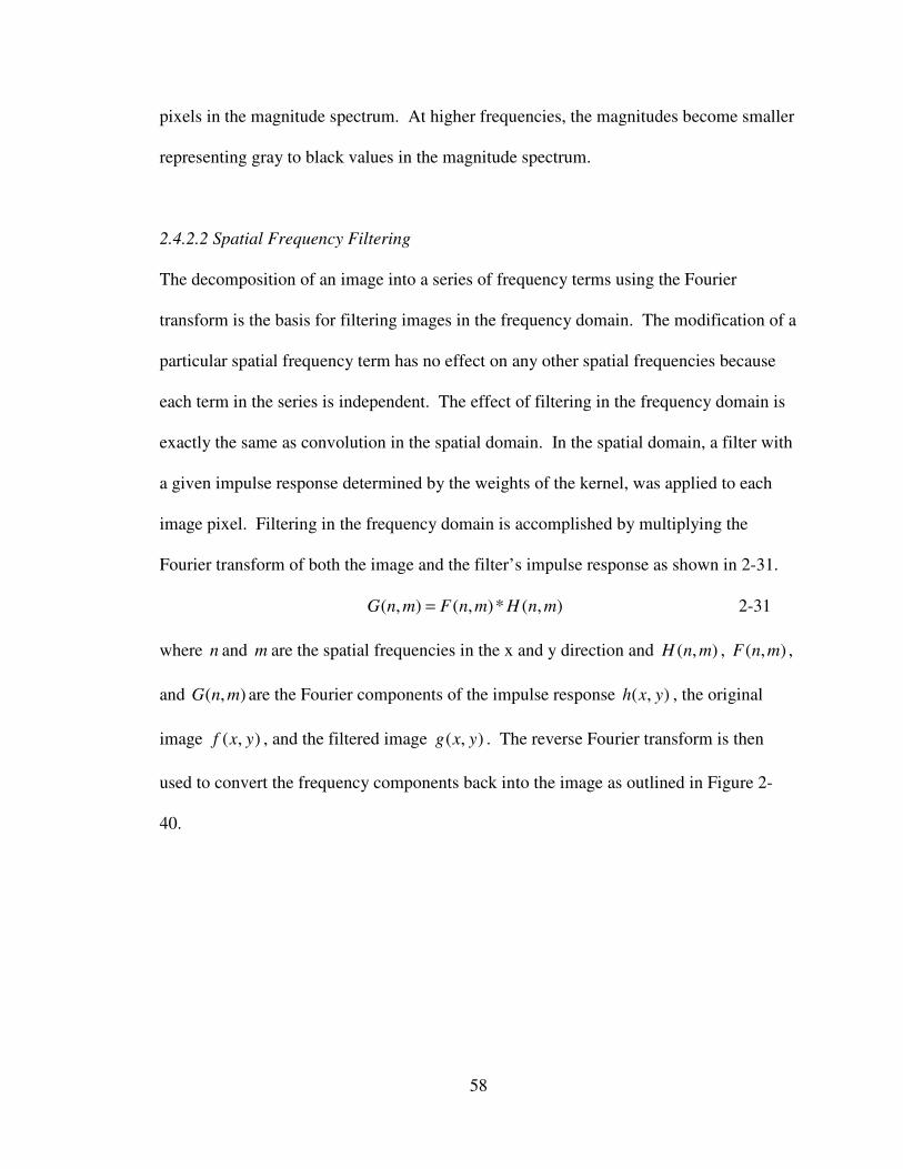
58
pixels in the magnitude spectrum. At higher frequencies, the magnitudes become smaller
representing gray to black values in the magnitude spectrum.
2.4.2.2 Spatial Frequency Filtering
The decomposition of an image into a series of frequency terms using the Fourier
transform is the basis for filtering images in the frequency domain. The modification of a
particular spatial frequency term has no effect on any other spatial frequencies because
each term in the series is independent. The effect of filtering in the frequency domain is
exactly the same as convolution in the spatial domain. In the spatial domain, a filter with
a given impulse response determined by the weights of the kernel, was applied to each
image pixel. Filtering in the frequency domain is accomplished by multiplying the
Fourier transform of both the image and the filter’s impulse response as shown in 2-31.
( , ) ( , )* ( , )G n m F n m H n m= 2-31
where n and m are the spatial frequencies in the x and y direction and ),( mnH , ),( mnF ,
and ),( mnG are the Fourier components of the impulse response ),( yxh , the original
image ),( yxf , and the filtered image ),( yxg . The reverse Fourier transform is then
used to convert the frequency components back into the image as outlined in Figure 2-
40.
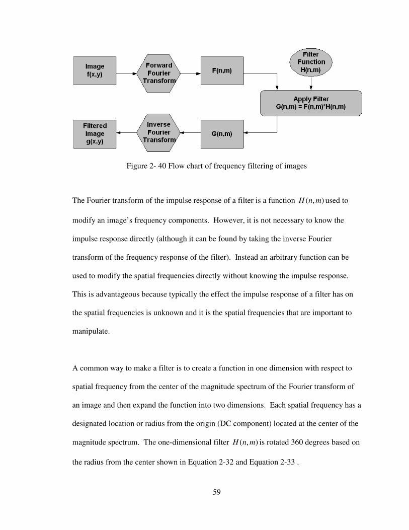
59
Figure 2- 40 Flow chart of frequency filtering of images
The Fourier transform of the impulse response of a filter is a function ),( mnH used to
modify an image’s frequency components. However, it is not necessary to know the
impulse response directly (although it can be found by taking the inverse Fourier
transform of the frequency response of the filter). Instead an arbitrary function can be
used to modify the spatial frequencies directly without knowing the impulse response.
This is advantageous because typically the effect the impulse response of a filter has on
the spatial frequencies is unknown and it is the spatial frequencies that are important to
manipulate.
A common way to make a filter is to create a function in one dimension with respect to
spatial frequency from the center of the magnitude spectrum of the Fourier transform of
an image and then expand the function into two dimensions. Each spatial frequency has a
designated location or radius from the origin (DC component) located at the center of the
magnitude spectrum. The one-dimensional filter ),( mnH is rotated 360 degrees based on
the radius from the center shown in Equation 2-32 and Equation 2-33 .

60
( , ) ( )H n m H ρ= 2-32
where
2 2 2n mρ = + 2-33
to create a circular filter. The phase components of the frequency terms must be
preserved in order to ensure an inverse Fourier transform can transform the image in the
frequency domain back to the spatial domain. The only requirement to be a phase
preserving filter is that the values of ),( mnH must be real. The filter values are
multiplied by both the real and imaginary parts of the Fourier Transform corresponding
to spatial frequency component. The circular property of the filter ensures that the same
filter value is applied to all phase components at a given spatial frequency.
The filter function typically ranges from 0 to 1 over the range of spatial frequencies
present in the image (DC component or zero frequency to the Nyquist frequency). If the
filter function has a value of zero, this essentially changes the magnitude at the
corresponding spatial frequency to zero or no modulation. If the filter function has a
value of 1, the modified magnitude at the corresponding frequency is equal to the original
magnitude.
2.4.2.2.1 Filtering Techniques
The most common filters are low-pass, high-pass, and band-pass. A low-pass filter
attenuates high frequencies while passing low frequencies. The effect of low-pass filters
is the same as convolution in the spatial domain with simple averaging kernel weights.
The image loses sharp edges and fine details and essentially blurs the image because the
higher frequency information is subtracted from the image. The most common filter is

61
the ideal low-pass filter where frequencies below a cutoff frequency cf are allowed to
pass and the frequencies above cf are blocked. The ideal low-pass filter has no transition
period from passing to attenuation of frequencies and can be described for the one and
two dimensional cases in Equation 2-34.
2 2
2 2
1 1( ) ( , )
0 0
c c
c c
for f f for n m fH f H n m
for f f for n m f
≤ + ≤
= → = > + >
2-34
Figure 2- 41 shows the magnitude spectrum of a one dimensional ideal low-pass filter
and Figure 2- 42 shows the one dimensional filter rotated 360 degrees about n and m in
the x and y directions to create a two dimensional filter for an image size of 640 x 480.
Figure 2- 41 One-dimensional low pass filter
Figure 2- 42 Two-dimensional low pass filter

62
The magnitude spectrum of the two dimensional filter is designed to coincide with the
magnitude spectrum of Fourier transform of the image which is commonly displayed
with the DC component in the center and distance from the center corresponding to an
increase in spatial frequency. The ideal low-pass filter starts at 1 at the lowest frequency
and drops to 0 at a desired frequency cf .
Ideal low-pass filters create a finite discontinuity in the magnitude spectrum and therefore
create a finite discontinuity in the Fourier transformed image. The truncation of the
Fourier spectral components at the cutoff frequency introduce artifacts commonly called
ringing when the filtered image is transformed back into the spatial domain [Weeks
1997]. To illustrate the concept of ringing an ideal low pass filter was applied to Figure
2- 1 to create Figure 2- 43.
Figure 2- 43 Example of ringing artifacts
An ideal low pass filter was applied to Figure 2- 1 to produce the artifacts that appear in
Figure 2- 43.

63
To circumvent the effect of ringing at sharp discontinuities a smooth edge can be applied
at the transition point of the low-pass filter. There are several common filter functions
used in digital image processing such as a parabolic or cosine function. The most
appropriate function is the Gaussian shape because the filter never drops to zero but
leaves a long tail beyond the cutoff frequency. The inverse Fourier transform of the
Gaussian filter is another Gaussian filter which would eliminate the effect of ringing. It
is also common to use the discrete approximation to the Gaussian filter known as the
Butterworth filter to produce the same effect. It is important to note that only the
magnitude spectrums of these filters can be used in image processing due to the phase
preserving requirements.
The magnitude of the Butterworth filter is described by Equation 2-35:
12
( ) 1
n
c
DH D C
D
− = +
2-35
where D is the distance from the center of the filter or the zero frequency to a particular
frequency and cD is the distance to the nominal filter cutoff value cf . Again, ultimately
this distance corresponds to a specific spatial frequency. The constant C is commonly set
to 1 or 0.414 to set the magnitude of the filter at the nominal filter cutoff value to 50% or
21 respectively. The integer n is the order of the filter commonly 1 or 2. The higher
the function order, the steeper the filter profile. Figure 2- 44 displays three Butterworth
filter curves with common cutoff distances (frequencies) and Figure 2- 45 displays
different function orders.
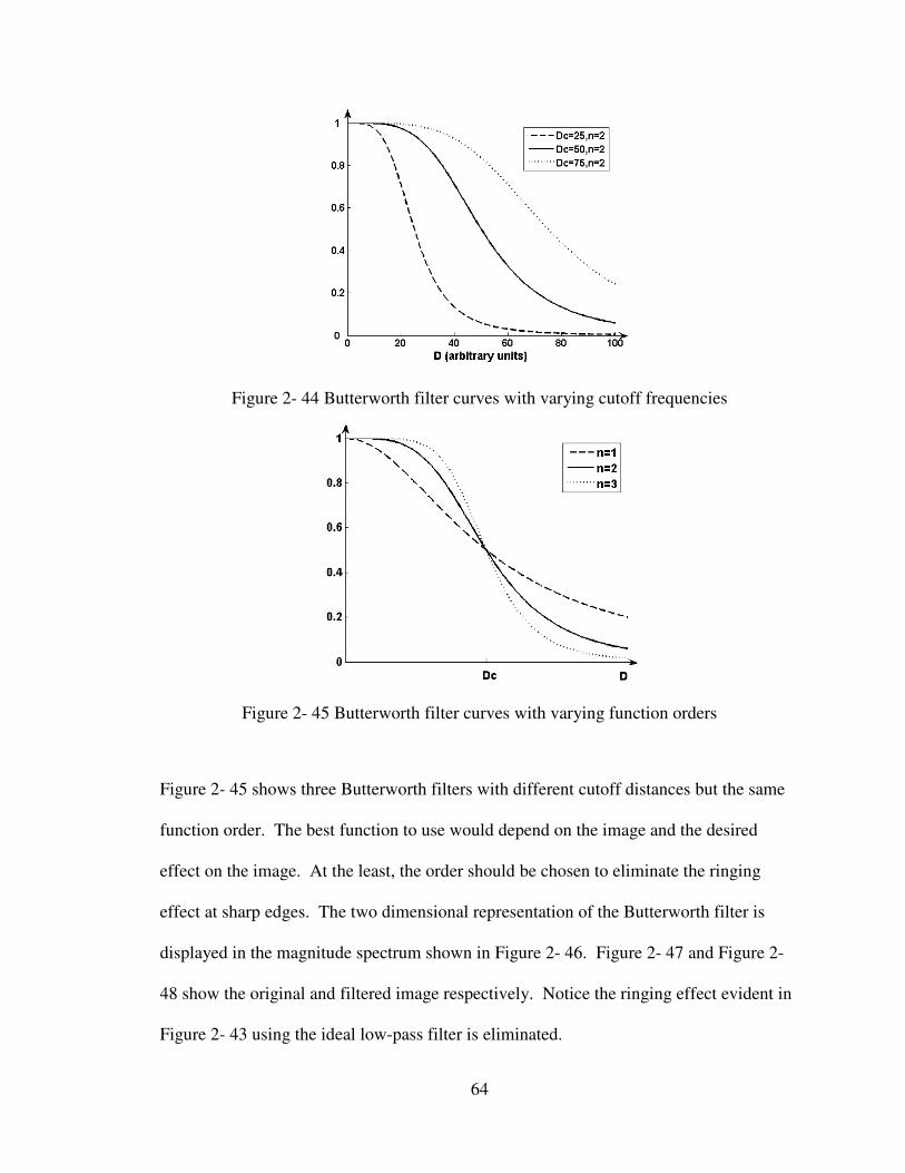
64
Figure 2- 44 Butterworth filter curves with varying cutoff frequencies
Figure 2- 45 Butterworth filter curves with varying function orders
Figure 2- 45 shows three Butterworth filters with different cutoff distances but the same
function order. The best function to use would depend on the image and the desired
effect on the image. At the least, the order should be chosen to eliminate the ringing
effect at sharp edges. The two dimensional representation of the Butterworth filter is
displayed in the magnitude spectrum shown in Figure 2- 46. Figure 2- 47 and Figure 2-
48 show the original and filtered image respectively. Notice the ringing effect evident in
Figure 2- 43 using the ideal low-pass filter is eliminated.

65
Figure 2- 46 Magnitude spectrum of 2-D Butterworth filter
Figure 2- 47 Original Image

66
Figure 2- 48 Image modified using Butterworth filter
High-pass filters pass high frequency information and attenuate low frequency
information. The filters previously discussed for low-pass can be modified to create high
pass filters. When applying a high-pass filter, the edges of image features are retained
but the overall detail of the image is lost. To illustrate the effect of a high-pass filter,
consider a high-pass Butterworth filter described by Equation 2-36.
12
( ) 1
n
cDH D C
D
−
= +
2-36
and represented in two dimensions in Figure 2- 49.

67
Figure 2- 49 High Pass 2-D Butterworth filter
The result of applying this filter to Figure 2- 47 is shown in Figure 2- 50.
Figure 2- 50 Image processed with high pass Butterworth filter
Notice the edges at sharp brightness differences are retained in the filtered images shown
by the outline in components such as the computer screen, PCU, and the lamp. It is

68
important to note that when using high pass filters the average overall brightness of an
image is usually kept the same. Therefore the filter magnitude at the DC level is left
unchanged.
Finally, band-pass filters are used to attenuate or pass a particular band of spatial
frequencies of interest. A common procedure for noise removal is to analyze the
magnitude spectrum for peaks at frequencies where there is periodic or unwanted noise.
These frequencies can simply be subtracted from an image by applying a filter function
that equals zero at these frequencies. The filter functions used for band-pass filters are
equivalent to those used for low and high pass filters. The edges of the bands can be
sharp like the ideal filter or smooth like Gaussian or Butterworth filter.

69
Chapter 3: Human Perception Experimental Design
3.1 Approach
To understand the effect TIC display quality has on human perception, fire fighters were
given a typical TIC task: identifying a fire hazard by observing an IR image. A series of
images were presented to the test subjects, which were a representative sample of fire
fighters that regularly use TIC, on well-characterized computer screens in an
ergonomically designed perception laboratory. The images were adjusted to
quantitatively degrade image contrast, brightness, noise level, and spatial resolution.
These image quality parameters were labeled the primary factors. Robustness factors,
such as the amount of thermal clutter, the type of thermal scene, the shape and relative
location of the fire hazards within the image were added to the image test matrix to
control for variables that could potentially affect the results. The matrix of images
presented to the test subjects was statistically constructed using a Taguichi experimental
design so that it was possible to deconvolve the results to understand the interactions of
the primary factors and their weighted effect on perception. Using the results of this
study, a model was developed to predict a fire fighter’s probability of successfully
completing the recognition task given the key primary factors. A pilot study, using NIST
personnel, was conducted as a proof of concept and to aid in the design of the full scale
test.
The project was investigated through the collaboration between the National Institute of
Standards and Technology (NIST), the Fire Protection Engineering Program at the
University of Maryland, and the Army’s Night Vision Laboratory (NVL).

70
3.2 Night Vision Laboratory (NVL)
NVL is a military laboratory at Fort Belvoir in Virginia that is dedicated to the research
and development of night vision technology for military applications. As part of NVL’s
mission, a perception lab is devoted to testing soldiers’ ability to identify and recognize
targets based on the information gained from a thermal image. NVL evaluates military
tasks such as recognizing and identifying ships, weapons, explosives and video clips of
threatening human movements based on thermal imaging of the scenario.
Because of NVL’s experience in human testing and data collection methods, NVL’s
ergonomically designed perception lab was an ideal environment to conduct the testing
on fire fighter task performance. The lab included ten test stations with 12-bit cathode
ray tube (CRT) monitors that differentiate 4096 levels of gray, far greater than a standard
monitor that distinguish only 256 gray levels. The CRT grid was also more fine then the
grid of the TIC system. Therefore the CRT grid adequately sampled the image and
therefore any impact of resolution was not due to the screens at NVL but the resolution of
the imaging system. Sampling is critical to avoid aliasing artifacts. For a more detailed
discussion of the sampling of system resolution refer to work done by Boreman
[Boreman 2001].
Each station was equipped with sufficient lighting, comfortable chairs and temperature
control to create an ideal comfortable atmosphere and windowless to avoid glare issues.

71
3.3 Image Production
3.3.1 Hazards
The study was designed to investigate the ability to identify fire hazards in office and
living room scenes that fire fighters are trained to understand and accustomed to viewing
with a TIC. Hazards such as hotspots in walls, overheated electrical equipment, hot
wires, and buried hot spots in furniture were used to simulate a smoldering or flaming fire
in early stages where there would be no visual evidence of a flame or the origin of smoke.
According to fire fighters trained in TIC, one of the most common reasons fire
department are called to a scene is because building occupants smell smoke but cannot
determine the origin. Fire fighters use TIC to scan the room.
One hazard type that was used for this study was a faulty connection in an electrical
system that caused a low-resistance connection such as a wire, to carry a large amount of
current to a source not equipped to handle the voltage. Figure 3- 1 displays infrared
images of overheated electrical outlets.
Figure 3- 1 Overheated electrical outlets

72
Overheated wiring or devices could occur for various reasons such as lightning strikes
sending current through an electrical system, poor connections, or uninsulated wiring.
Another common occurrence of overheated wires occurs when a table or desk leg crushes
a wire and causes a considerable amount of resistance heating as shown Figure 3- 2.
Figure 3- 2 Crushed wire under table leg
Other hazards used for this study included buried hot spots in trash cans and furniture as
shown in Figure 3- 3.
Figure 3- 3 Buried hotspot in chair

73
Buried hazards were used to represent a cigarette or match that was thrown away or
dropped which has the potential to be slow developing and could elude a building
occupant of the origin of the burning.
Although this experiment focused on one of the most common applications of TIC, it is
important to note that TIC are used in a dynamic range of environments and applications.
Due to a number of limiting factors, other scenarios and uses of TIC were beyond the
scope of this work.
As an alternative to physically creating wall fires, buried hazards and short circuiting
electrical devices, external heat sources were used to simulate the effect the radiation
from the actual hazards would have on the TIC detectors. Heat rope and heat tape, which
are essentially high resistance wires, were used to reproduce over heated wires and
receptacles. To reproduce a generic hot spot, a high intensity halogen lamp and heat guns
were used. The intent of this work was only to replicate the radiation emitted from a real
hazard on a TIC display screen and not to reproduce the hazards.
A balance between the realism of the hazards and a controlled experiment was necessary.
Fire fighters must be able to positively identify realistic fire hazards and at the same time
create controlled images to focus the experiment on image quality parameters and
conditions that could influence detection probability. To ensure the validity of the
thermal images and the type of hazards, the images were sent to fire fighters who train
others on the applications and techniques used for TIC in the field. In addition, the

74
feedback from the pilot study images was used to tweak the types of images used for the
real perception experiment.
3.3.2 Scene
A small one compartment structure was constructed to be a representative room or office
a fire fighter could encounter. A 12’ by 12’ room was built from gypsum wallboard
backed by 2 x 4 constructional lumber at 16” on center spacing. Electrical outlets,
overhead lights, wall lamps, and carpet were installed in the room.
The room was furnished with living room furniture on two walls and office equipment on
the other two walls to capture two scenes with one room to reduce construction costs.
Figure 3- 4 and Figure 3- 5 displays the living room scene assembled on two walls and
Figure 3- 6 and Figure 3- 7 displays the office work station.

75
Figure 3- 4 Living room scene

76
Figure 3- 5 Living room scene
Figure 3- 6 Office scene

77
Figure 3- 7 Office scene
Common living furniture such as tables, chairs, and standing lamps were added to the
living room scene. Other items such as candles, lamps, plants, coffee cups, etc were also
added as thermal clutter. The office work station included desks and computer chairs as
well as computers, monitors, coffee makers, surge protectors, battery chargers among
other electronic equipment.
3.3.3 Image Capturing
The images were captured using a FLIR Systems ThermaCam P640 commercial infrared
camera. The display image quality of the FLIR P640 was chosen because it had far better
display image quality than any fire fighting TIC available on the market. Most
commercial fire fighting TIC have detectors with 320 x 240 or 160 x 120 pixel arrays.

78
The ThermaCam P640 has a detector pixel array of 640 x 480, four times the resolution
of fire fighting TIC. Each detector pixel can distinguish 16-bit of information. In other
words, the image produced on the display considers 65536 different intensity values or
graylevels to create the image. A fire fighting TIC typically uses an 8-bit or 256
graylevel scale.
3.4 Defining the Scenario Criteria
3.4.1 Robustness Factors
Robustness factors were included in the test design to ensure the conclusions of the study
would apply to a broad range of scenarios. There were a total of four robustness factors
that included, hazard position, hazard type, thermal clutter, and scene type which were
considered the most important factors that may influence the results according to pilot
study results. The number of levels associated with each hazard and the definition of
these levels are shown in Table 3- 1 .

Robustness Factor
1 Target Position
2 Hazard Type
3 Amount of Clutter
4 Scene
One hazard type was used in each image (except for images with no hazard) in one of
five locations as shown in
79
Table 3- 1 Robustness Definitions
Robustness Factor Number
of Levels Level Definition
6 Center
Upper Left
Upper Right
Lower Left
Lower Right
No Target
5 1 Overheated receptacle
2 Overheated wire
3 Buried hotspot in furniture/ trash
can
4 Small hotspot in wall
5 Large hotspot in wall
2 Small: 2-5 thermal objects
Large: 8-10 thermal objects
2 Office work station
Living room
One hazard type was used in each image (except for images with no hazard) in one of
locations as shown in Figure 3- 8.
Figure 3- 8 Hazard location divisions
Level Definition
1 Overheated receptacle
3 Buried hotspot in furniture/ trash
wall
5 Large hotspot in wall
5 thermal objects
10 thermal objects
One hazard type was used in each image (except for images with no hazard) in one of
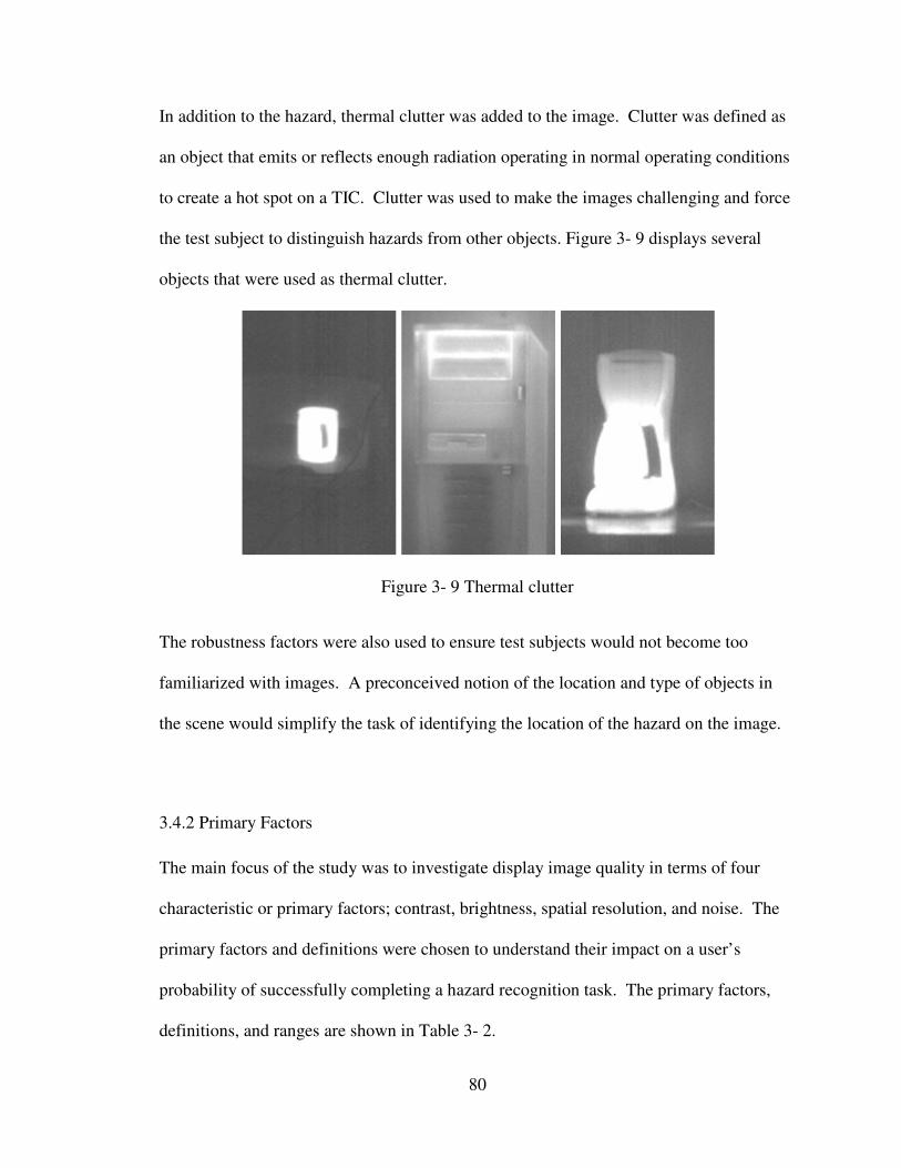
80
In addition to the hazard, thermal clutter was added to the image. Clutter was defined as
an object that emits or reflects enough radiation operating in normal operating conditions
to create a hot spot on a TIC. Clutter was used to make the images challenging and force
the test subject to distinguish hazards from other objects. Figure 3- 9 displays several
objects that were used as thermal clutter.
Figure 3- 9 Thermal clutter
The robustness factors were also used to ensure test subjects would not become too
familiarized with images. A preconceived notion of the location and type of objects in
the scene would simplify the task of identifying the location of the hazard on the image.
3.4.2 Primary Factors
The main focus of the study was to investigate display image quality in terms of four
characteristic or primary factors; contrast, brightness, spatial resolution, and noise. The
primary factors and definitions were chosen to understand their impact on a user’s
probability of successfully completing a hazard recognition task. The primary factors,
definitions, and ranges are shown in Table 3- 2.

81
Table 3- 2 Primary Factor Definitions
Image
Characteristic
Definition Range
Min Max
Contrast anceluContrast minσ= 0 ∞
Brightness anceluBrightness minµ= 0 ∞
Spatial
Resolution
)(0
NEMMTFSRA
curve −= ∫ where A= intersection of
MTF and NEM
0 pixelcycles
f nyquist 5.0=
Noise µ
σ noiseityNonuniform = 0 ∞
The results of this study must have a connection to the NIST test methods to establish the
minimum requirements for the image quality parameters in NFPA 1801, Standard for
Thermal Imagers for the Fire Service. Conceptually, the perception experiment was
designed to find the minimum image quality for a user to perform a task and the NIST
test methods evaluate a TIC ability to reproduce an equivalent image quality. The
definitions used to quantify image quality in terms of contrast, brightness, spatial
resolution, and noise are equivalent in both cases but these parameters are evaluated on
dissimilar images. However, conceptually we are still evaluating the same principal; the
ability of a TIC to distinguish relatively hot and cold objects and the ability of a user to
distinguish relatively light and dark objects.
As discussed in Section 1.3.2 Bench-Scale Test Methods Developed by NIST, contrast,
brightness, and spatial resolution are evaluated using a controlled thermal image of a
heated bar target over an ambient background. In the perception experiment, the
parameters are evaluated over images of heated realistic objects in an ambient scene. In a
similar fashion, nonuniformity is evaluated in the NIST test method as the random

82
fluxuations of pixel intensities from a uniform blackbody. In the perception experiment,
random fluxuations were simply added to the images to produce similar false variations
in pixel intensity. The perception experiment makes the connection between the user and
the image while the NIST test methods make the connection from the image to the TIC
resulting in a relationship between the user and the TIC.
3.5 Defining the Image Set
3.5.1 Restrictions
An image matrix was methodically constructed to ensure that each image contained a
combination of the primary and robustness factors and so that statistically it was possible
to extract the interactions between the factors and determine the weighted effect of each
factor on detection probability. The number of observations that could be completed in
one day was deemed to be 1250 according to recommendations made by the staff at NVL
that have experience conducting similar experiments that took a period of days. 1250
observations per day minimized the fatigue and boredom, human factors that could
influence test results. The total number of images or “observations” was restricted to
5,000 so that the test could be completed in four day window (1250 observations per day
* 4 days) to maximum the number of fire fighters and thus increasing the sample size for
more valid statistical data.
3.5.2 Pristine Image Set
All combinations of the robustness factors were considered in a full factorial matrix to
create a “pristine” image set that did not include image degradation from the primary

83
factors. From Table 3- 1, multiplying the number of levels for each robustness factor
leads to 6 x 5 x 2 x 2 or 120 settings. In addition to a full factorial, one half of the images
were “replicated”, for a total of 180 images. Replication for this experiment did not
mean identical images but rather the replicated images had the same robustness settings.
The 180 pristine images were created from the FLIR ThermaCam. The detailed image
set is shown in Appendix A.
3.5.3 Primary Factor Design Points
A subset of an mk Factorial Grid was driven by a Taguchi L25 Orthogonal Design to
create the combinations (design points) of primary factors. A total of approximately 27
design points were possibly to satisfy the 5,000 image constraint (5000 total images / 180
pristine images~ 27 design points). A 54 grid design or five levels at each of the four
primary factors consists of 625 design points. The Taguichi L25 Orthogonal subset of
the grid consists of only 25 design points, meeting the 27 point restriction while retaining
orthogonality. Orthogonality is important to ensure no correlation between any two
factors and therefore each design point is independent providing different information
improving the efficiency of the results (Sanchez 2007).
The 25 design points are shown in Table 3- 3.

84
Table 3- 3 Design Points
Factor Settings
Design
Point Contrast Brightness
Spatial
Resolution Noise
1 0.4000 0.5015 0.0284 0.3333
2 0.4000 3.6339 0.0522 0.2000
3 0.4000 6.7696 0.0760 0.1429
4 0.4000 9.9021 0.0998 0.1111
5 0.4000 13.0346 0.1234 0.0909
6 0.9330 0.5015 0.0522 0.1429
7 0.9330 3.6339 0.0760 0.1111
8 0.9330 6.7696 0.0998 0.0909
9 0.9330 9.9021 0.1234 0.3333
10 0.9330 13.0346 0.0284 0.2000
11 1.4669 0.5015 0.0760 0.0909
12 1.4669 3.6339 0.0998 0.3333
13 1.4669 6.7696 0.1234 0.2000
14 1.4669 9.9021 0.0284 0.1429
15 1.4669 13.0346 0.0522 0.1111
16 1.9993 0.5015 0.0998 0.2000
17 1.9993 3.6339 0.1234 0.1429
18 1.9993 6.7696 0.0284 0.1111
19 1.9993 9.9021 0.0522 0.0909
20 1.9993 13.0346 0.0760 0.3333
21 2.5317 0.5015 0.1234 0.1111
22 2.5317 3.6339 0.0284 0.0909
23 2.5317 6.7696 0.0522 0.3333
24 2.5317 9.9021 0.0760 0.2000
25 2.5317 13.0346 0.0998 0.1429
A pilot study was conducted using NIST personnel to get an idea of the amount of image
degradation in terms of the four primary factors was necessary to impact the hazard
detection probability. The TIC display quality test methods in NFPA 1801 require the
TIC to produce an image that would yield a detection probability of 95% [NFPA 1801].
Using the results of the pilot study, the 25 design points were chosen to fine tune the
settings of the images to capture a high probability of hazard detection ranging between

85
50-95%. Using a focused range of image settings, more data could be collected within
the range of interest.
3.5.4 Calculations
3.5.4.1 Contrast and Brightness
Contrast is the standard deviation of the 640 x 480 2-D luminance array of the image
captured with the FLIR Thermacam corresponding to the image as it would be seen on
the monitors at NVL.
[ ]1 1
2
0 0
1( , )
M N
y x
contrast c f x y BNM
− −
= =
= = −∑∑ 3-1
where B is the brightness or mean luminance as
1 1
0 0
1( , )
M N
y x
brightness B f x yNM
− −
= =
= = ∑∑ 3-2
and N and M are 640 and 480 respectively.
3.5.4.2 Spatial Resolution
The spatial resolution of an imaging system over all spatial frequencies from 0 (DC or
zero modulation) to the nyquist frequency (the highest spatial frequency that can encoded
in a digital image) is defined by the MTF as described in Chapter 2 Section
2.3.3 Spatial Resolution. The MTFA, a single number value to describe the spatial
resolution of an imaging system is found by integrating the area under the MTF curve
between the MTF and the NEM of the imaging system.

86
To generate an MTF or a known frequency response for the images used in this study, a
low-pass Butterworth filter (a discrete approximation to the Gaussian filter) was applied
to the 2-D Fourier Transforms of the pristine images. The Butterworth filter was chosen
because it offered the ability to control the attenuation rate of the filter for increasing
frequency components. In addition, the filter changes from the pass band to the
attenuation band without producing ringing artifacts in the filter image as common in
other filters such as the ideal lowpass filter.
The Butterworth filter reduces the modulation depth at increasing spatial frequencies of
each pristine image according to specified slope properties as described in
Section2.4.2.2.1 Filtering Techniques. The design points for spatial resolution used for
this study were dependent on the nominal cutoff frequency (Dc) of the low-pass
Butterworth filter. For design points 1, 10, 14, 18 and 22 the nominal cutoff frequency
was set to 0.02 ������
���� . The constant C was set to 1 to adjust the magnitude of the
filter at the nominal filter cutoff value to 50%. The integer n was set to 2. The
magnitude of the Butterworth filter H(D) which when multiplied by the pristine image to
create the MTF of the degraded image is shown in Equation 3-3.
1 12 4
( ) 1 ( ) 10.02
n
c
D fH D C MTF f
D
− − = + → = +
3-3
To calculate the MTFA, the NEM is also required. The NEM was calculated using the
methods described in NFPA 1801 section 8.1.5 specifically for the FLIR camera used to
capture the IR images in this study. The dimensionless value is 0.02861. The final step

87
is to define the bounds of the integration for the MTFA by calculating the intersection of
the MTF and the line created by the NEM as described in Section
2.3.3 Spatial Resolution. To find the intersection, both equations were set to be equal to
each other and solved for the frequency.
14
1 0.02861 0.0482780.02
f cyclesf
pixel
−
+ = → =
3-4
The MTFA is then
140.048278
0
140.048278 0.048278
0 0
( ) 1 0.028610.02
1 0.02861 0.02030.02
fMTFA f
f cyclespixel
−
−
= + − =
+ − =
∫
∫ ∫
3-5
The MTFA must then be converted from cycles/pixel to a universal unit of frequency,
cycles/mrad because cycles/pixel is dependent on the imaging system’s detector array.
The detector array typically does not fill the enter cell or pixel area. The ratio of the
active detector element to the actual cell is known as the fill factor. A finite fill factor
affects the resolution of the imaging system [Lloyd 1979]. If the frequency of target is
high enough to fit between the active detector elements there will be no output from the
imaging system.
Although cycles/mrad is a universal frequency unit, the conversion factor from
cycles/pixel to cycles/mrad is unique to a specific camera at a specific distance away
from the target. To calculate the conversion factor for the FLIR camera used for this
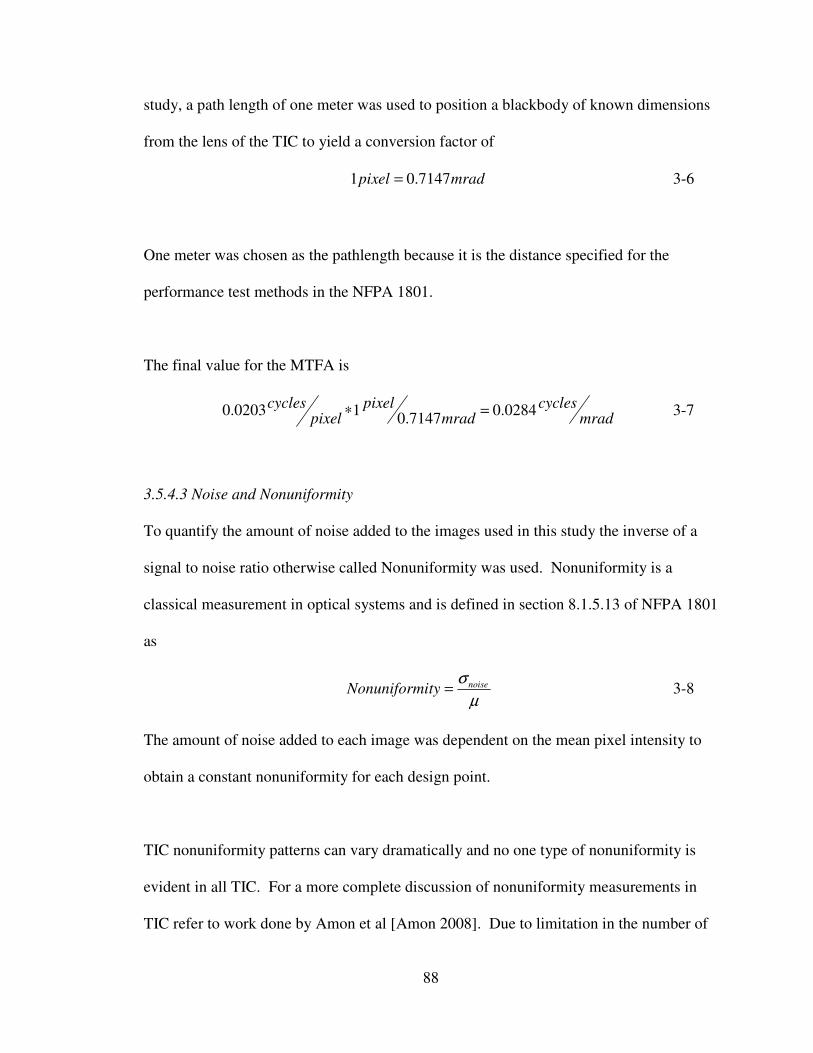
88
study, a path length of one meter was used to position a blackbody of known dimensions
from the lens of the TIC to yield a conversion factor of
1 0.7147pixel mrad= 3-6
One meter was chosen as the pathlength because it is the distance specified for the
performance test methods in the NFPA 1801.
The final value for the MTFA is
0.0203 1 0.02840.7147
cycles pixel cyclespixel mrad mrad
∗ = 3-7
3.5.4.3 Noise and Nonuniformity
To quantify the amount of noise added to the images used in this study the inverse of a
signal to noise ratio otherwise called Nonuniformity was used. Nonuniformity is a
classical measurement in optical systems and is defined in section 8.1.5.13 of NFPA 1801
as
noiseNonuniformityσ
µ= 3-8
The amount of noise added to each image was dependent on the mean pixel intensity to
obtain a constant nonuniformity for each design point.
TIC nonuniformity patterns can vary dramatically and no one type of nonuniformity is
evident in all TIC. For a more complete discussion of nonuniformity measurements in
TIC refer to work done by Amon et al [Amon 2008]. Due to limitation in the number of

89
images and factors that could be included in this study, all types of nonuniformity where
not investigated. A Gaussian distributed noise was added to the pristine image to act as a
general nonuniformity.
A Gaussian distribution was chosen because it was the most common type of electronic
noise present in cameras and sensors (Weeks 1996). It is often also used to model
unknown additive noise sources from different parts of the image system. By the central
limit theorem, the sum of a large number of independent noise sources approaches
Gaussian distributed noise [Smith 2007].
3.6 Image Processing
Due to the interactions of the image degradation techniques used to manipulate each of
the primary factors to create an image with specific values for contrast, brightness, spatial
resolution and noise, the order of image processing was critical. Image processing is
typically used to improve not degrade the quality of images. Techniques such as
frequency filtering effect many image characteristics, specifically contrast and noise.
While a low-pass filter such as the Butterworth was used in this study to reduce and
remove the higher frequency components to blur the images and generate a frequency
response (MTF) of the image, the filter also decreased the contrast and adjusted the noise
of an image.
Low pass filtering limits the span of graylevels used to create the image. Blurring
reduces sharp edges and therefore the contrast [Russ 2002]. Sharp distinctions in
graylevels between objects in an image correspond to a high contrast. As the image

90
becomes blurry due to a low pass filter, the span of graylevels used to create the objects
in the images shrink, reducing contrast.
To circumvent the interactions of contrast and filtering for this study an iterative
approach was use to find a balance that would create an image that met the design points
for both the contrast and spatial resolution as shown in Figure 3- 10. The contrast and
brightness of the images were adjusted first to meet their design points. The low pass
Butterworth filter was then applied to the image to adjust the MTF of the image. The
contrast and brightness were then readjusted so that at the end of the process each
primary factor met the desired design point. Up until this point in the image processing
program, noise was not introduced into the image.
The quantity of noise in the final images was assumed to only be a result of the additive
Gaussian noise. Although all images have noise, the amount of noise present in the
images before the application of noise was assumed to be negligible to the amount of
desired Gaussian noise added. Noise is hard to quantify unless there are obvious spikes
in the magnitude spectrum of the Fourier transform of the image that do not contribute to
the quality of the image but random fluxuations in the image signal.
To further justify this assumption, the application of the low-pass Butterworth filter
removed the high frequency signal components. At higher spatial frequencies the
magnitude of the frequency response is not due to the quality of the camera but the
random pixel to pixel variations associated with noise [Russ 2002]. The Butterworth

91
filter eliminated the high frequencies in particular the frequencies above the intersection
of the MTF and the NEM. Any frequency response of the image above the NEM is due
to noise and not the quality of the image. For these reasons, noise was the last
component added to the image set. A flow chart of the image processing is shown in
Figure 3- 10.

92
Figure 3- 10 Flowchart of image processing

93
To implement the degradation process outlined in Figure 3- 10, Matlab R2006b Version
7.3.0 was used to write a program to manipulate the pristine images to meet each of the
25 design points. The complete custom made program can be found in Appendix B
Image Processing Program. An example of how this program manipulated one of the
images from the pristine image set to meet each of the 25 design points can be found in
Appendix D.

94
Chapter 4: Modeling Human Perception
4.1 Objective
Create a model to predict the probability of a fire fighter successfully completing a
hazard recognition task with the aid of only an IR image.
4.2 Test Subjects
A group of sixteen TIC users of varying age, fire fighting experience, TIC experience and
skill level were used to capture data from a representative portion of the fire fighting
community to help identify any bias in the test results that could link test subject
performance with experience. A list of fire fighter backgrounds can be seen in Appendix
C Test Subject Background.
The test subjects were required to attend an informative session which included a Power
Point presentation followed by a hazard training exercise on the NVL testing program.
The Power Point presentation described the project goals as well as the types of scenes,
thermal clutter, and hazards that would be seen in the images. Because of the diversity of
the fire fighter’s training backgrounds, to avoid possible confusion, test subjects were
given a training exercise that included pristine images similar to the types of scenes that
would be seen in the actual study. The test subjects were required to select the hazard in
each of the training images. Only test subjects who scored a 100% on the training
exercise were allowed to proceed to the real study to ensure any wrong answers could be
attributed to the image quality and not the definition of a hazard. The training program

95
also familiarized the test subjects on how to navigate through the images and select the
hazards using NVL’s testing program.
4.3 Experiment
The test was conducted in NVL’s ergonomically designed perception laboratory using
their testing system as well their procedures to avoid any impact on a test subject’s
performance that could not be attributed to the image quality. The experiment included
4500 images split up into 25 sessions containing 180 images each. The images were
presented in a strategic order by progressively improving the quality of the images to
minimize the effect of learning during the tests. The ranking of design point order was
chosen based on pilot study results.
Time limitation was not a variable. Each image was presented on the screen for an
unlimited amount of time until a selection was made. A five minute break was required
between each of the sessions to avoid fatigue and boredom which could potentially
influence their alertness and performance on the study.
The test subjects were asked to view each of the images and located the hazard via a
mouse click on the screen. A “No Hazard” selection box was also incorporated on the
test screen for images without a hazard. The user’s mouse click location was compared
to the actual hazard location. If the mouse click was within the coordinates of the hazard
a correct answer was registered by NVL’s program. A ‘1’ indicated a correct answer and
a ‘0’ represented incorrect. The program automatically consolidated each test subject’s
test results in a comma delimited text file that included the test subject ID, the mouse

96
click coordinates on the screen, the result of the selection, and the time to make the
decision.
4. 4 Data
Several of the 16 user’s were unable to complete the entire test, therefore, rather than
4,500 x 16 = 72,000 data points, only 54,540 points were recorded. These data points
were binary; either a 1 for correct response or 0 for incorrect response. Each data point
corresponded to a design point (1-25) for contrast, brightness, spatial resolution, and
nonuniformity. The average probability of successfully identifying a fire hazard for each
design points is summarized in Figure 4- 1.
Figure 4- 1 Average response for design points
It is important to note that the design points were not ranked based on difficulty.
1 2 3 4 5 6 7 8 9 10 11 12 13 14 15 16 17 18 19 20 21 22 23 24 25
Design Point/Image Setting
0.0
0.2
0.4
0.6
0.8
1.0
Ave
rag
e R
esp
on
se

97
4. 5 Logistic Regression Model
When the response variable is binary, the response function often follows the shape of a
logistic regression function. This model is typically sigmoidal and monotonic having a
stretched “S” (increasing) or reverse “S” (decreasing) shaped response with asymptotes at
0 and 1 and takes on the following form (Agresti, 1990).
exp( ' )
1 exp( ' )
Xp
X
β
β
∧
=+
4-1
The probability of success is predicted based on X which can be any number of input
parameters. X in this study corresponded to the primary factors to define image quality:
contrast, brightness, spatial resolution, and nonuniformity. Several versions of the model
were considered including the primary factors only, the primary factors plus two terms
interactions, and primary factors plus all interactions. The primary factors are shown in
Table 4- 1.
Table 4- 1Primary Factors
Variable Description
X1 Contrast
X2 Brightness
X3 Spatial Resolution
X4 Nonuniformity (noise)
Based on the diagnostics discussed later in this section, a modification to the primary
factors plus two term interaction multiple logistic regression model was chosen. The
coefficients of each parameter, β , are regression coefficients typically calculated using
computer-intensive numerical search procedures. For a more detailed description of how

98
the coefficient values are produced refer to work done by Neter et al (Neter, Kutner,
Nachtsheim, &Wasserman, 1996). The calculated regression coefficients are shown in
Table 4- 2.
Table 4- 2 Multiple logistic regression coefficients
Coefficient Description Value Std. Error t-value
β0 Intercept -1.030 0.140 -7.346
β1 Contrast 0.076 0.040 1.929
β2 Brightness -0.172 0.008 -20.220
β3 Spatial Resolution 0.991 0.343 2.893
β4 Noise 44.510 2.238 19.885
β5 Contrast-Brightness Interaction 0.169 0.005 36.195
β6 Contrast-Noise Interaction -12.350 0.708 -17.449
β7 Brightness-Spatial Resolution Interaction -0.216 0.027 -7.975
β8 Brightness-Noise Interaction -1.597 0.108 -14.753
β9 Spatial Resolution-Noise Interaction -16.935 3.947 -4.291
Expanding Equation 4-1 to account for two term interactions
1 2 3 4
1 2 1 4 2 3 2 4 3 4
1 2 3 4
1 2 1 4 2 3 2 4 3 4
exp( 1.030 0.076 0.172 0.991 44.510
0.169 12.350 0.216 1.597 16.935 )
1 exp( 1.030 0.076 0.172 0.991 44.510
0.169 12.350 0.216 1.597 16.935 )
X X X X
X X X X X X X X X Xp
X X X X
X X X X X X X X X X
∧
− + − + +
+ − − − −=
+ − + − + +
+ − − − −
4-2
Given constant values for the primary factors X1, X2, X3, and X4, the probability of
successfully identifying the target in the images is predicted by p∧
.
4.6 Cross Validation
A cross validation study was used to compare the performance of various versions of the
logistic regression model. From the original dataset of 54,540 points, two thirds of the
records from each image set was randomly selected to create the modeling dataset, and

99
the remaining one third of the records from each design point was used as a validation
dataset. The process is displayed in Figure 4- 2.
Figure 4- 2 Formation of modeling and validating datasets
Using the modeling dataset, several model structures were considered including primary
factors only, primary factors with two term interactions minus the contrast-spatial
resolution, primary factors with all two term interactions, and primary factors with all
interactions. Each model was used to get an estimate of the probability of successfully
completing the recognition task of the validating dataset. The difference between the
empirical value and the predicted values are calculated at each image setting. The
process was repeated 100 times and the results are shown in Figure 4- 3 through Figure 4-
6 and summarized in Figure 4- 7.

100
Figure 4- 3 Main effects only
Figure 4- 4 Main effects + all two term interactions
-0.3
-0.25
-0.2
-0.15
-0.1
-0.05
0
0.05
0.1
0.15
0.2
0 5 10 15 20 25
Em
pir
ica
l V
alu
e -
Pre
dic
ted
Va
lue
Image Setting
-0.2
-0.15
-0.1
-0.05
0
0.05
0.1
0.15
0 5 10 15 20 25
Em
pir
ica
l V
alu
e -
Pre
dic
ted
Va
lue
Image Setting
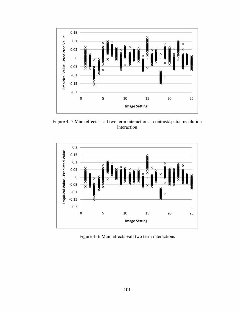
101
Figure 4- 5 Main effects + all two term interactions - contrast/spatial resolution
interaction
Figure 4- 6 Main effects +all two term interactions
-0.2
-0.15
-0.1
-0.05
0
0.05
0.1
0.15
0 5 10 15 20 25
Em
pir
ica
l V
alu
e -
Pre
dic
ted
Va
lue
Image Setting
-0.2
-0.15
-0.1
-0.05
0
0.05
0.1
0.15
0.2
0 5 10 15 20 25
Em
pir
ica
l V
alu
e -
Pre
dic
ted
Va
lue
Image Setting

102
Figure 4- 7 Average deviation from observed values
The main effect plus 2 term interactions as well as subsequent models with additional
parameters show significant improvement upon the main effect only model. The average
greatest deviation over 100 trials from the observed data and the model incorporating
main effects plus two term interactions was 11.3%. The data also shows that the main
effect plus all interaction model had an average greatest deviation of 10.8%. Since the
model with additional terms did not offer a substantial gain over models with less
parameters, it was discarded.
-0.25
-0.2
-0.15
-0.1
-0.05
0
0.05
0.1
0.15
0.2
0 5 10 15 20 25
Av
era
ge
( E
mp
iric
al
Va
lue
-P
red
icte
d V
alu
e)
Image Setting
Main Effects Only
Main Effect + 2 term int
Main Effect + 2 term int - contrast/spatial res
Main Effect + all ints

103
4.7 Model Deviance and Partial Deviance
When creating a logistical regression model, the model deviance and partial deviance can
be informative tests in determining the number factors contributing to the model fit. The
deviance of a fitted model determines the relationship of the fitted model to the model
that fits all n observations perfectly, otherwise known as the saturated model (Neter,
Kutner, Nachtsheim, & Wasserman, 1996). The partial deviance is the difference
between the model deviances for two fitted models and is used to determine if a reduced
fitted model is comparable to a larger model. When the partial deviance is small, the
reduced parameter model provides a similar fit to that of the larger model (Neter, Kutner,
Nachtsheim, & Wasserman, 1996). When the number of data points, n, is reasonably
large, as in our case, the partial deviance follows approximately a chi-squared distribution
with p-q degrees of freedom; where p is the number of parameters in the larger model,
and q the number of parameters in the subset model.
The first test is to determine if the any of the primary factors Xi, do not contribute to the
model fit; or in other words, do βq = βq+1 = … = βp-1 = 0? A partial deviance test was
conducted between the null model, a model that simply relies on a constant, to the
expanded modeling incorporating the primary factors.
The selected model, shown in Equation 4-2, incorporated all the primary factors plus two
term interactions less contrast- spatial resolution interactions.
� ����, �� , … , ��� = 68,979.70

104
Comparing this model deviance, in a partial deviance test, to that of the null model where
� ����� = 73,057.14, we can see a significant improvement to the model fit.
� ���� , … , ��|��� = 73,057.14 − 68,979.70 = 4,077.44
With a chi-square critical value of %.�&;�( = 16.92, we can strongly reject the null
hypothesis that β1 = β2 = … = β9 = 0.
A further look at the partial deviance between the model with primary factors plus all two
term interactions versus the subset model used in this study shows the additional contrast-
spatial resolution interaction term, corresponding to the coefficient β10 , does not provide
additional improvement on the model fit.
� �����|��, �� , … , ��� = 68,979.70 − 68,979.70 = 0
With a chi-square critical value of %.�&;�( = 3.84, we can accept the null hypothesis that
β10 =0.
4.8 Informal Goodness of Fit Test
For a fitted multiple logistic regression model to be appropriate, the shape of the
estimated response function must be monotonic and sigmoidal; key properties of a
logistic response function. To perform an Informal Goodness of Fit Examination records
with similar fitted values,π∧
, are grouped into a number of classes (typically between 5
and 10) with approximately the same number of n observations. Within each class, the
estimated proportion of 1s, denoted by pj, is calculated for all n. These values are then
plotted against the midpoint of the fitted values for each class. Table 4- 3 and Figure 4- 8

105
display the Informal Goodness of Fit data, using five classes, for the selected human
perception model.
Table 4- 3 Informal Goodness of Fit Test with 5 Classes
Class j *+ Interval Midpoint nj pj
1 0.222 , 0.507 0.364 10912 0.409
2 0.507 , 0.562 0.534 10904 0.532
3 0.562 , 0.671 0.617 10908 0.612
4 0.671 , 0.724 0.698 10916 0.736
5 0.724 , 0.779 0.751 10900 0.749
Figure 4- 8 Diagnostic plot of estimated proportions with 5 classes
Figure 4- 8 clearly indicates the model is monotonic, and sigmoidal in nature. Expanding
the Informal Goodness of Fit Test to seven classes yields the following result shown in
Table 4- 4 and Figure 4- 9.
0.0
0.2
0.4
0.6
0.8
1.0
0.0 0.2 0.4 0.6 0.8 1.0
p
Fitted Value

106
Table 4- 4 Informal Goodness of Fit Test using 7 Classes
Class j *+ Interval Midpoint nj pj
1 0.222 , 0.486 0.354 7798 0.380
2 0.486 , 0.546 0.516 7790 0.522
3 0.546 , 0.570 0.558 7792 0.536
4 0.570 , 0.671 0.621 7796 0.593
5 0.671 , 0.719 0.695 7784 0.735
6 0.719 , 0.736 0.727 7792 0.738
7 0.736 , 0.779 0.757 7788 0.750
Figure 4- 9 Diagnostic plot of estimated proportions using 7 classes
Again, Figure 4- 9 suggests that a monotonic, sigmoidal relationship is tenable.
0.000
0.100
0.200
0.300
0.400
0.500
0.600
0.700
0.800
0.900
1.000
0.000 0.200 0.400 0.600 0.800 1.000
p
Fitted Values

107
4.9 Chi-Square Goodness of Fit Test
The Informal Goodness of Fit Test can be extended into a formal Chi-Square Goodness
of Fit Test provided the observations are independent and the sample size is large. This
test provides the ability to detect large departures from the logistic response function.
Similarly, to the Informal Goodness of Fit Test, the records are again divided into classes
of approximately equal size with similar fitted values,π∧
. The number of observed
successes (1’s) and failures (0’s) are denoted by Oj1 and Oj0, respectively. If the logistic
response function is appropriate, the expected number of successes within a class will be
equal to the sum of the fitted values for that class; likewise, the number of failures will be
equal to the sum of 1 − ,- . This leads to the Chi-Square Goodness of Fit Test statistic:
( )
21
2
1 0
cjk jk
i k jk
O E
Eχ
= =
−=∑ ∑ 4-3
with decision rules:
If �( ≤ %(�1 − /; � − 2�, conclude H0 , logistic response appropriate
If �( > %(�1 − /; � − 2�, conclude Ha , logistic response not appropriate
The classes, observed and expected number of successes and failures for the calculation
of the test statistic are displayed in Table 4- 5.

108
Table 4- 5 Goodness of Fit Test
Class
j *+ Interval nj
Number of Failures Number of Successes
Observed
Oj0
Expected
1 2 − *+
Observed
Oj1
Expected
1 *+
1 0.222 , 0.507 10912 6447 6426.54 4465 4485.46
2 0.507 , 0.562 10904 5101 5004.68 5803 5899.32
3 0.562 , 0.671 10908 4230 4098.98 6678 6809.02
4 0.671 , 0.724 10916 2878 3139.85 8038 7776.16
5 0.724 , 0.779 10900 2739 2724.96 8161 8175.04
The test statistic for the selected human perception model is calculated as:
�( = �6447 − 6426.54�(
6426.54 + �4465 − 4485.46�(
4485.46 + ∙∙∙ + �2739 − 2724.96�(
2724.96
+ �8161 − 8175.04�(
8175.04 = 41.04
The critical value is found to be %.�&;5( = 7.81, thus the null hypothesis of the logistic
response function being appropriate is rejected. The associated p-value with this test is
6.40 x 10⁻⁹
.
4.10 Deviance Goodness of Fit Test
Given a large sample size, n, the model deviance, � �6��, �� , … , �78�9, will follow
approximately a chi-square distribution with n – p degrees of freedom if the logistic
response function is correct. The decision rules for the deviance goodness of fit test are:
If � �6��, �� , … , �78�9 ≤ %(�1 − /; : − ��, conclude H0 , logistic response
appropriate
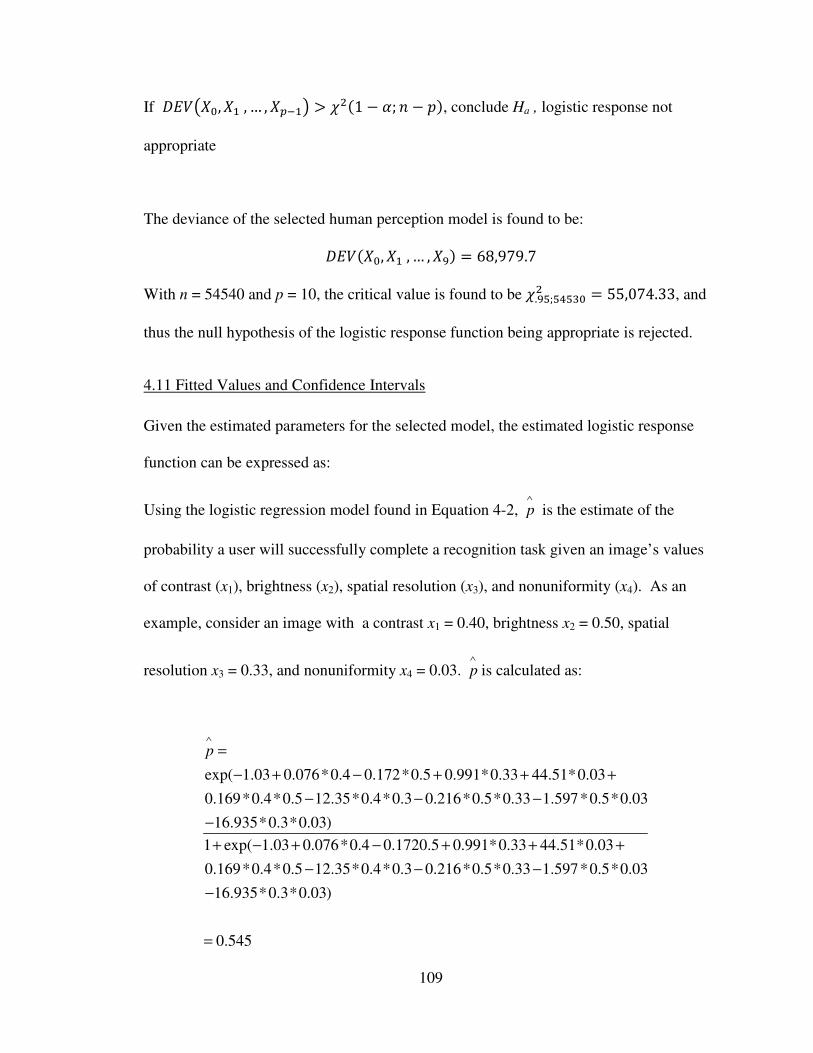
109
If � �6��, �� , … , �78�9 > %(�1 − /; : − ��, conclude Ha , logistic response not
appropriate
The deviance of the selected human perception model is found to be:
� ����, �� , … , ��� = 68,979.7
With n = 54540 and p = 10, the critical value is found to be %.�&;&;&5�( = 55,074.33, and
thus the null hypothesis of the logistic response function being appropriate is rejected.
4.11 Fitted Values and Confidence Intervals
Given the estimated parameters for the selected model, the estimated logistic response
function can be expressed as:
Using the logistic regression model found in Equation 4-2, p∧
is the estimate of the
probability a user will successfully complete a recognition task given an image’s values
of contrast (x1), brightness (x2), spatial resolution (x3), and nonuniformity (x4). As an
example, consider an image with a contrast x1 = 0.40, brightness x2 = 0.50, spatial
resolution x3 = 0.33, and nonuniformity x4 = 0.03. p∧
is calculated as:
exp( 1.03 0.076*0.4 0.172*0.5 0.991*0.33 44.51*0.03
0.169*0.4*0.5 12.35*0.4*0.3 0.216*0.5*0.33 1.597*0.5*0.03
16.935*0.3*0.03)
1 exp( 1.03 0.076*0.4 0.1720.5 0.991*0.33 44.51*0.03
0.169*0.4*0.5 12.3
p∧
=
− + − + + +
− − −
−
+ − + − + + +
− 5*0.4*0.3 0.216*0.5*0.33 1.597*0.5*0.03
16.935*0.3*0.03)
0.545
− −
−
=

110
With an estimated regression function there is uncertainty in the parameters. This
uncertainty leads to uncertainty in the fitted value, p∧
. One way to capture this
uncertainty is in the form of a confidence interval about the fitted value. The lower, L,
and upper, U, (1 – α)% confidence interval values for p∧
are found by:
{ }
{ }
' ' 2
(1 /2)
' ' 2
(1 /2)
exp( )
1 exp( )
b X z X s b XL
b X z X s b X
α
α
−
−
−=
+ − 4-4
{ }
{ }
' ' 2
(1 /2)
' ' 2
(1 /2)
exp( )
1 exp( )
b X z X s b XU
b X z X s b X
α
α
−
−
+=
+ + 4-5
where b is the vector of regression coefficients provided in Table 4- 2;
X is the vector of predictor variable terms, to include interactions terms:
{1, x1, x2, x3, x4, x1x2, x1x4, x2x3, x2x4, x3x4, };
z6�8= (� 9 is the inverse of the standard normal cumulative distribution at 61 −α 2� 9%;
and @ABCD is the variance-covariance matrix for the regression parameters found
to be:
@ABCD =
0.020 -0.004 -0.001 -0.041 -0.280 0.000 0.082 0.001 0.011 0.370
-0.004 0.002 0.000 0.008 0.051 0.000 -0.020 0.000 -0.001 -0.068
-0.001 0.000 0.000 0.001 0.002 0.000 0.000 0.000 0.000 0.003
-0.041 0.008 0.001 0.117 0.521 0.000 -0.135 -0.003 -0.018 -1.038
-0.280 0.051 0.002 0.521 5.010 0.008 -1.472 0.000 -0.207 -6.288
0.000 0.000 0.000 0.000 0.008 0.000 -0.002 0.000 0.000 -0.006
0.082 -0.020 0.000 -0.135 -1.472 -0.002 0.501 0.001 0.058 1.510
0.001 0.000 0.000 -0.003 0.000 0.000 0.001 0.001 0.000 -0.030
0.011 -0.001 0.000 -0.018 -0.207 0.000 0.058 0.000 0.012 0.173
0.370 -0.068 0.003 -1.038 -6.288 -0.006 1.510 -0.030 0.173 15.577

111
The variance-covariance matrix is calculated using statistical computer programs and will
not be discussed further here. Please refer to work by Neter et al (Neter, Kutner,
Nachtsheim, &Wasserman, 1996).
For the considered example of contrast x1 = 0.40, brightness x2 = 0.50, spatial resolution
x3 = 0.33, and nonuniformity x4 = 0.03, the lower and upper 95% confidence bounds for
p∧ = 0.545 can be calculated as:
CEF =
GHHHHHHHHI −1.03
0.076−0.1720.991
44.5100.169
−12.350−0.216−1.597
−16.935JKKKKKKKKL
E
GHHHHHHHHI 10.400.500.330.030.200.010.170.010.01J
KKKKKKKKL
= 0.1835; FE@ABCDF =
GHHHHHHHHI 10.400.500.330.030.200.010.170.010.01J
KKKKKKKKL
E
@ABCD
GHHHHHHHHI 10.400.500.330.030.200.010.170.010.01J
KKKKKKKKL
= 0.0015;
z6�8�.�& (� 9 = z��.�M&� = 1.96;
Hence:
N = exp60.1835 − 1.96√0.001591 + exp60.1835 − 1.96√0.00159 = 0.526 and
V = exp60.1835 + 1.96√0.001591 + exp60.1835 + 1.96√0.00159 = 0.565

112
Chapter 5: Summary and Conclusions
5.1 Summary of Model Fit
The chosen model function to estimate the probability of successfully identifying the
target utilizes the main effects (contrast, brightness, spatial resolution, and noise) plus
two term interactions less the spatial resolution/contrast interaction term. Through a
cross validation study, this model’s prediction never deviated more than approximately
11% from the observed data. A more complex model, utilizing all interaction terms, only
improved the model fit by less than 1%.
Of all the models compared in this study, the selected model was chosen because it was
the simplest form (least amount of terms) while offering the most accurate results. The
selected function showed significant improvement over a constant model as indicated by
the partial deviance test. In addition, the Informal Goodness of Fit test suggests that the
response function follows a sigmoidal and monotonic shape, key indicators of the validity
of using a logistic response function to model binary response data. Although further
diagnostic testing, using the Chi-Squared Goodness of Fit Test and the Deviance
Goodness of Fit test, debunk the use of a logistic response function to characterize the
data, there is no one statistical test that offers concrete evidence. With the use of
confidence intervals, the uncertainty in the model can be characterized and therefore the
failed goodness of fit tests should not be justification to eliminate the model.
5.2 Recommendation for Model Use in NFPA 1801
One of the most important findings of this study was that the interactions between
contrast, spatial resolution, brightness, and noise in an image have a greater effect on

113
human perception than any one variable by itself. When considering test methods to
adequately characterize the ability of a TIC to produce a quality image, interactions must
be accounted for.
The predictions made by the fitted model will be more conservative when using the
lowest primary factors measurements in the NIST test methods. As discussed in 1.3.2
Bench-Scale Test Methods Developed by NIST, contrast, brightness, spatial resolution,
and nonuniformity (noise) are calculated from many images captured, from thermal
targets over a range of temperatures, and the measurements will vary. Since the test
methods are designed to investigate temperatures indicative of actual scenarios, the TIC
must be required to provide adequate image quality over the entire range. The method by
which the model should be used is outlined below. For additional details on these
procedures refer to the draft of NFPA 1801 [NFPA 1801 2008].
1. Perform Image Recognition Test (spatial resolution). Calculate the contrast and
CTF at each numbered step (predetermined bar frequency), from lowest to highest
step number, on the spatial resolution target shown in Figure 1- 2. Also, calculate
the average brightness of the pixels used in the contrast calculation.
a. The contrast calculated at step 2 is X1 and is held constant.
b. The brightness calculated at step 2 is X2 and is held constant.
c. Convert the CTF measurement, using the bar frequency at each step, to the
MTF as defined by the procedures outlined in this work in Table 3- 2. The
result is the spatial resolution, X3 and will vary in value from step to step.

114
2. The nonuniformity test is independent. It is calculated over a temperature range
from 0 to 260C. The maximum nonuniformity at any of the set point
temperatures is deemed the nonuniformity of the imaging system as a
conservative estimate for X4 in the model. This value is held constant.
3. For the above data collected at each numbered step on the Image Recognition
Test target, plug in the values for contrast (X1), brightness (X2), spatial resolution
(X3), and noise (X4).
a. Use the model to calculate p∧
at each numbered step.
4. Note that the Nonuniformity Test in step 2 need be conducted only one time. The
noise value (X4), can be used in all further image quality testing.
These procedures, as outlined in the draft form of NFPA 1801, are conducted over a
range of temperatures. NIST and the NFPA technical committee will have to make a
decision as to what value for p∧
indicates acceptable performance by a TIC.
5.3 Future Work
This study was the first attempt at trying to model the relationship between TIC image
quality and fire fighter task performance and therefore there is an extensive list of future
possibilities to further improve the model. One suggestion would be to create a more
diverse set of images expanding further into the TIC applications such as images
incorporating flames, water mist, steam, and smoke. Expanding from still images, three
dimensional images of a scene could provide a user interactive test offering the ability of
the test subjects to scan a 3-D image. Incorporating dynamic motion videos, could
further the realism of the imagery set.

115
The statistical analysis of the dataset could also be expanded. The logistic regression
model used to fit the data found in the perception experiment is a class of generalized
linear models. This approach transforms the response by use of a link function, which
relates the linear combination of the predictor variables to the mean response. One may
consider an approach using a generalized additive model. The generalized additive
model also considers a link function, but rather than a linear combination of the predictor
values, it considers a linear combination of functions of the predictor values.
Although the user and robustness factors were not considered in the creation of this
model, as they cannot be controlled in real-world scenarios, their impact and the
improvement they may bring to the model could be investigated. Such an investigation
may lead to insights and improvements in system use and training.

116
Appendices
Appendix A
Robustness Factors - (Levels)
Pristine
ID
Target Position
(6)
Hazard
Type (5) Clutter (2) Scene (2)
1 Center (C) 1 Small Office
2 Upper Left (UL) 1 Small Office
3 Upper Right (UR) 1 Small Office
4 Lower Left (LL) 1 Small Office
5 Lower Right (LR) 1 Small Office
6 No Target (N) 1 Small Office
7 Center (C) 2 Small Office
8 Upper Left (UL) 2 Small Office
9 Upper Right (UR) 2 Small Office
10 Lower Left (LL) 2 Small Office
11 Lower Right (LR) 2 Small Office
12 No Target (N) 2 Small Office
13 Center (C) 3 Small Office
14 Upper Left (UL) 3 Small Office
15 Upper Right (UR) 3 Small Office
16 Lower Left (LL) 3 Small Office
17 Lower Right (LR) 3 Small Office
18 No Target (N) 3 Small Office
19 Center (C) 4 Small Office
20 Upper Left (UL) 4 Small Office
21 Upper Right (UR) 4 Small Office
22 Lower Left (LL) 4 Small Office
23 Lower Right (LR) 4 Small Office
24 No Target (N) 4 Small Office
25 Center (C) 5 Small Office
26 Upper Left (UL) 5 Small Office
27 Upper Right (UR) 5 Small Office
28 Lower Left (LL) 5 Small Office
29 Lower Right (LR) 5 Small Office
30 No Target (N) 5 Small Office
31 Center (C) 1 Large Office
32 Upper Left (UL) 1 Large Office
33 Upper Right (UR) 1 Large Office
34 Lower Left (LL) 1 Large Office
35 Lower Right (LR) 1 Large Office
36 No Target (N) 1 Large Office
37 Center (C) 2 Large Office

117
38 Upper Left (UL) 2 Large Office
39 Upper Right (UR) 2 Large Office
40 Lower Left (LL) 2 Large Office
41 Lower Right (LR) 2 Large Office
42 No Target (N) 2 Large Office
43 Center (C) 3 Large Office
44 Upper Left (UL) 3 Large Office
45 Upper Right (UR) 3 Large Office
46 Lower Left (LL) 3 Large Office
47 Lower Right (LR) 3 Large Office
48 No Target (N) 3 Large Office
49 Center (C) 4 Large Office
50 Upper Left (UL) 4 Large Office
51 Upper Right (UR) 4 Large Office
52 Lower Left (LL) 4 Large Office
53 Lower Right (LR) 4 Large Office
54 No Target (N) 4 Large Office
55 Center (C) 5 Large Office
56 Upper Left (UL) 5 Large Office
57 Upper Right (UR) 5 Large Office
58 Lower Left (LL) 5 Large Office
59 Lower Right (LR) 5 Large Office
60 No Target (N) 5 Large Office
61 Center (C) 1 Small Living
62 Upper Left (UL) 1 Small Living
63 Upper Right (UR) 1 Small Living
64 Lower Left (LL) 1 Small Living
65 Lower Right (LR) 1 Small Living
66 No Target (N) 1 Small Living
67 Center (C) 2 Small Living
68 Upper Left (UL) 2 Small Living
69 Upper Right (UR) 2 Small Living
70 Lower Left (LL) 2 Small Living
71 Lower Right (LR) 2 Small Living
72 No Target (N) 2 Small Living
73 Center (C) 3 Small Living
74 Upper Left (UL) 3 Small Living
75 Upper Right (UR) 3 Small Living
76 Lower Left (LL) 3 Small Living
77 Lower Right (LR) 3 Small Living
78 No Target (N) 3 Small Living
79 Center (C) 4 Small Living
80 Upper Left (UL) 4 Small Living
81 Upper Right (UR) 4 Small Living
82 Lower Left (LL) 4 Small Living
83 Lower Right (LR) 4 Small Living

118
84 No Target (N) 4 Small Living
85 Center (C) 5 Small Living
86 Upper Left (UL) 5 Small Living
87 Upper Right (UR) 5 Small Living
88 Lower Left (LL) 5 Small Living
89 Lower Right (LR) 5 Small Living
90 No Target (N) 5 Small Living
91 Center (C) 1 Large Living
92 Upper Left (UL) 1 Large Living
93 Upper Right (UR) 1 Large Living
94 Lower Left (LL) 1 Large Living
95 Lower Right (LR) 1 Large Living
96 No Target (N) 1 Large Living
97 Center (C) 2 Large Living
98 Upper Left (UL) 2 Large Living
99 Upper Right (UR) 2 Large Living
100 Lower Left (LL) 2 Large Living
101 Lower Right (LR) 2 Large Living
102 No Target (N) 2 Large Living
103 Center (C) 3 Large Living
104 Upper Left (UL) 3 Large Living
105 Upper Right (UR) 3 Large Living
106 Lower Left (LL) 3 Large Living
107 Lower Right (LR) 3 Large Living
108 No Target (N) 3 Large Living
109 Center (C) 4 Large Living
110 Upper Left (UL) 4 Large Living
111 Upper Right (UR) 4 Large Living
112 Lower Left (LL) 4 Large Living
113 Lower Right (LR) 4 Large Living
114 No Target (N) 4 Large Living
115 Center (C) 5 Large Living
116 Upper Left (UL) 5 Large Living
117 Upper Right (UR) 5 Large Living
118 Lower Left (LL) 5 Large Living
119 Lower Right (LR) 5 Large Living
120 No Target (N) 5 Large Living
121 Upper Left (UL) 1 Small Office
122 Upper Right (UR) 1 Small Office
123 Lower Right (LR) 1 Small Office
124 Center (C) 2 Small Office
125 Upper Left (UL) 2 Small Office
126 Lower Left (LL) 2 Small Office
127 Center (C) 3 Small Office
128 Lower Right (LR) 3 Small Office
129 No Target (N) 3 Small Office

119
130 Center (C) 4 Small Office
131 Lower Left (LL) 4 Small Office
132 No Target (N) 4 Small Office
133 Upper Left (UL) 5 Small Office
134 Upper Right (UR) 5 Small Office
135 Lower Right (LR) 5 Small Office
136 Center (C) 1 Large Office
137 Lower Left (LL) 1 Large Office
138 No Target (N) 1 Large Office
139 Upper Right (UR) 2 Large Office
140 Lower Right (LR) 2 Large Office
141 No Target (N) 2 Large Office
142 Upper Left (UL) 3 Large Office
143 Upper Right (UR) 3 Large Office
144 Lower Left (LL) 3 Large Office
145 Upper Left (UL) 4 Large Office
146 Upper Right (UR) 4 Large Office
147 Lower Right (LR) 4 Large Office
148 Center (C) 5 Large Office
149 Lower Left (LL) 5 Large Office
150 No Target (N) 5 Large Office
151 Center (C) 1 Small Living
152 Lower Left (LL) 1 Small Living
153 No Target (N) 1 Small Living
154 Upper Right (UR) 2 Small Living
155 Lower Right (LR) 2 Small Living
156 No Target (N) 2 Small Living
157 Upper Left (UL) 3 Small Living
158 Upper Right (UR) 3 Small Living
159 Lower Left (LL) 3 Small Living
160 Upper Left (UL) 4 Small Living
161 Upper Right (UR) 4 Small Living
162 Lower Right (LR) 4 Small Living
163 Center (C) 5 Small Living
164 Lower Left (LL) 5 Small Living
165 No Target (N) 5 Small Living
166 Upper Left (UL) 1 Large Living
167 Upper Right (UR) 1 Large Living
168 Lower Right (LR) 1 Large Living
169 Center (C) 2 Large Living
170 Upper Left (UL) 2 Large Living
171 Lower Left (LL) 2 Large Living
172 Center (C) 3 Large Living
173 Lower Right (LR) 3 Large Living
174 No Target (N) 3 Large Living
175 Center (C) 4 Large Living

120
176 Lower Left (LL) 4 Large Living
177 No Target (N) 4 Large Living
178 Upper Left (UL) 5 Large Living
179 Upper Right (UR) 5 Large Living
180 Lower Right (LR) 5 Large Living

121
Appendix B Image Processing Program
Main Programs
%This program converts the temperature output (.mat) file from the %FLIR ThermaCam P640 to a 16-bit uncompressed image close all clear all
%Input a .mat file into Matlab im=input('What file would you like to load?\n'); im1=strcat(im,'.mat'); load(im1);
im2=input('What image you want to convert?No file extension\n');
%Find image size [ymax xmax]=size(im2);
%Find minimum and maximum temperature in file minimum=min(im2); minval=min(minimum); maximum=max(im2); maxval=max(maximum);
%Enter temperature range that produces best quality image temp1=input('What is the minimum temp\n'); temp2=input('What is the max temp\n');
image1=zeros(ymax, xmax);
%Normalize temperature data for i=1:xmax for j=1:ymax image1(j,i)=(im2(j,i)-minval)/(maxval-minval); end end
image2=zeros(ymax,xmax);
%Create a 16-bit grayscale with temperature data for q=1:i for r=1:j image2(r,q)=image1(r,q)*65535; end end
%Solve for variables needed to adjust image to correct grayscale p=((temp1+273.15)-minval)/(maxval-minval); xkcd=0; if p<0 p=0; xkcd=(minval-(273.15+temp1))/(temp2-temp1); end

122
z=((temp2+273.15)-minval)/(maxval-minval);
%Create 16 bit image from temperature data image3=uint16(image2);
%Adjust image to match desired gray-scale image4=imadjust(image3,[p,z],[xkcd,1]);
%Verify image is appropriate imshow(image4)
%Create filename filename = strcat(im,'.png');
%Save image as 16-bit uncompressed .png file imwrite(image4,filename,'png','BitDepth',16) %-------------------------------------------------------------------
%ImagePro is an image processing program to adjust the contrast, %brightness, spatial resolution, and noise of an image to meet the
% 25 design points clear all close all fprintf('Beginning LumImageProLoop')
%Image Counter ii=1; %Design Point Counter iii=1;
%Allocate memory conarray=zeros(4500,1); brightarray=zeros(4500,1); spatialarray=zeros(4500,1); noisearray=zeros(4500,1);
%Start outerloop to loop through 180 pristine images (image filenames
are %numerical labeled from 1 to 180)
while ii<=180
%Input Image name=num2str(ii); name1=strcat('image',name,'.png'); im = imread(name1);
%Convert the image to an array of numbers to manipulate im2=double(im);
%Find the size of the array [M N]=size(im2);
%Create an array of luminance data to describe the image as it will
appear

123
%on the test monitors at NVL lumimage=zeros(M,N); for j=1:M for k=1:N if im2(j,k)>8192 lumimage(j,k)=((1*10^-8)*((im2(j,k))^2))-
(0.0002*(im2(j,k)))+1.6159; elseif im2(j,k)<=8192 lumimage(j,k) = (3*(10^(-05)))*im2(j,k)+0.0266; else fprintf('ERROR\n') end end end
%Find the brightness of the original image in pixel intensity bright = round(mean(mean(im2))); %Find the corresponding luminance on NVL displays lumbright=round(mean(mean(lumimage)));
%Find the contrast of the original image in pixel intensity values=zeros(M,N); for j=1:M for k=1:N values(j,k)=((im2(j,k)-bright)^2); end end contrast=sqrt(mean(mean(values))); %Find the corresponding contrast on NVL display lumvalues=zeros(M,N); for j=1:M for k=1:N lumvalues(j,k)=((lumimage(j,k)-lumbright)^2); end end lumcontrast=sqrt(mean(mean(lumvalues)));
%Loop through all 25 design points counter=1; while counter<=25
%Input design point parameters if counter==1 stdcon=900; lumstdcon=0.4; newbright=12800; lumnewbright=0.5015; Wn=0.02; SNR=15.0; LumSNR=3.0;
elseif counter==2 stdcon=900; lumstdcon=0.4; newbright=27200; lumnewbright=3.6339;

124
Wn=0.0366; SNR=20.0; LumSNR=5.0;
elseif counter==3 stdcon=900; lumstdcon=0.4; newbright=33600; lumnewbright=6.7696; Wn=0.0533; SNR=25.0; LumSNR=7.0; elseif counter ==4 stdcon=900; lumstdcon=0.4; newbright=40000; lumnewbright=9.9021; Wn=0.07; SNR=30.0; LumSNR=9.0; elseif counter ==5 stdcon=900; lumstdcon=0.4; newbright=43200; lumnewbright=13.0346; Wn=0.0866; SNR=35.0; LumSNR=11.0; elseif counter ==6 stdcon=1500; lumstdcon=0.933; newbright=12800; lumnewbright=0.5015; Wn=0.0366; SNR=25.0; LumSNR=7.0; elseif counter ==7 stdcon=1500; lumstdcon=0.933; newbright=27200; lumnewbright=3.6339; Wn=0.0533; SNR=30.0; LumSNR=9.0; elseif counter ==8 stdcon=1500; lumstdcon=0.933; newbright=33600; lumnewbright=6.7696; Wn=0.07; SNR=35.0; LumSNR=11.0; elseif counter ==9 stdcon=1500; lumstdcon=0.933; newbright=40000; lumnewbright=9.9021;

125
Wn=0.0866; SNR=15.0; LumSNR=3.0; elseif counter ==10 stdcon=1500; lumstdcon=0.933; newbright=43200; lumnewbright=13.0346; Wn=0.02; SNR=20.0; LumSNR=5.0; elseif counter ==11 stdcon=2000; lumstdcon=1.4669; newbright=12800; lumnewbright=0.5015; Wn=0.0533; SNR=35.0; LumSNR=11.0; elseif counter ==12 stdcon=2000; lumstdcon=1.4669; newbright=27200; lumnewbright=3.6339; Wn=0.07; SNR=15.0; LumSNR=3.0; elseif counter ==13 stdcon=2000; lumstdcon=1.4669; newbright=33600; lumnewbright=6.7696; Wn=0.0866; SNR=20.0; LumSNR=5.0; elseif counter ==14 stdcon=2000; lumstdcon=1.4669; newbright=40000; lumnewbright=9.9021; Wn=0.02; SNR=25.0; LumSNR=7.0; elseif counter ==15 stdcon=2000; lumstdcon=1.4669; newbright=43200; lumnewbright=13.0346; Wn=0.0366; SNR=30.0; LumSNR=9.0; elseif counter ==16 stdcon=2500; lumstdcon=1.9993; newbright=12800; lumnewbright=0.5015; Wn=0.07;

126
SNR=20.0; LumSNR=5.0; elseif counter ==17 stdcon=2500; lumstdcon=1.9993; newbright=27200; lumnewbright=3.6339; Wn=0.0866; SNR=25.0; LumSNR=7.0; elseif counter ==18 stdcon=2500; lumstdcon=1.9993; newbright=33600; lumnewbright=6.7696; Wn=0.02; SNR=30.0; LumSNR=9.0; elseif counter ==19 stdcon=2500; lumstdcon=1.9993; newbright=40000; lumnewbright=9.9021; Wn=0.0366; SNR=35.0; LumSNR=11.0; elseif counter ==20 stdcon=2500; lumstdcon=1.9993; newbright=43200; lumnewbright=13.0346; Wn=0.0533; SNR=15.0; LumSNR=3.0; elseif counter ==21 stdcon=3000; lumstdcon=2.5317; newbright=12800; lumnewbright=0.5015; Wn=0.0866; SNR=30.0; LumSNR=9.0; elseif counter ==22 stdcon=3000; lumstdcon=2.5317; newbright=27200; lumnewbright=3.6339; Wn=0.02; SNR=35.0; LumSNR=11.0; elseif counter ==23 stdcon=3000; lumstdcon=2.5317; newbright=33600; lumnewbright=6.7696; Wn=0.0366; SNR=15.0;

127
LumSNR=3.0; elseif counter ==24 stdcon=3000; lumstdcon=2.5317; newbright=40000; lumnewbright=9.9021; Wn=0.0533; SNR=20.0; LumSNR=5.0; elseif counter ==25 stdcon=3000; lumstdcon=2.5317; newbright=43200; lumnewbright=13.0346; Wn=0.07; SNR=25.0; LumSNR=7.0; end
%Finding an initial guess for slope of linear point processing for
contrast slope=stdcon/contrast;
%Finding the y-intercept d as initial guess for the amount of increase
in %brightness d=newbright-bright;
%Wn is the nominal cutoff frequency used in a butterworth filter Wn = Wn*sqrt(M.^2+N.^2); %n defines the order of the butterworth equation of the slope of the
filter n=2;
countername=num2str(counter);
%fminsearch varies the values for the slope and d so that after the
spatial %resolution test all three parameters of the degraded image are as
desired
slopei = slope; %Initial guess for point processing of contrast and brightness X0 = [slopei,d];
options=optimset('TolX',1e+00,'Tolfun',1e+00); X = fminsearch(@Lumsearchfile, X0, options, im2, newbright, Wn, n,
contrast, bright,stdcon,lumbright,lumcontrast,lumstdcon,lumnewbright);
%Final slope and intercept values for contrast and brightness slope=X(1); d=X(2); %......................................................................
...

128
%ConBrighta manipulates contrast/brightness [contrastimage]= LumConbrighta(im2,slope,d,bright);
%Spatialresa adjusts the spatial resolution of the image using a
butterworth %filter in the frequency domain. [freqimage,Fplot,Gplot,newbright3,SR,contrastf, lumnewbright3,
lumcontrastf, Dmax]=LumSpatialresa(contrastimage,im2,Wn,n);
%fprintf('Your adjusted image has the following parameters\n') %fprintf('Your new contrast is %g\n',2*lumcontrastf/32.562) %fprintf('Your new brightness is %g\n',lumnewbright3/32.562) %fprintf('Your spatial resolution is %g\n', SR)
%Getting the desired nonuniformity by adding noise
%Find the amount of noise necessary to create the desired nonuniformity %Based on brightness DevVar1=newbright3/SNR; LumDevVar1=lumnewbright3/LumSNR;
%First guess Vari = 0.01; X0 = [Vari]; options=optimset('Tolfun',1e-06,'TolX',1e-06); X = fminbnd(@LumNoisesearch,0,0.1,options,
freqimage,DevVar1,LumDevVar1);
%Var is the final variance needed to reach the desired nonuniformity Var=X(1);
[noiseimage,lumDevNoise,lumnoisy]=LumNoise(freqimage,Var);
%Final Nonuniformity LumSNR1=lumnewbright3/lumDevNoise;
% fprintf('You deviation of noise is %g\n',DevNoise)
%Minor adjustment to get image back to 640x 480 %Add one more col and row noiseimage1=double(noiseimage); [q,p]=size(noiseimage1); toprow = noiseimage1(1,:); finalimage1 = [toprow;noiseimage1]; [q,p]=size(finalimage1); lastcol = finalimage1(:,p); finalimage = [finalimage1, lastcol];
%Put numbers back into 16-bit image finalimage=uint16(finalimage);

129
%Variable Output Names Wn1=num2str(Wn/sqrt(M.^2+N.^2)); n1=num2str(n);
Lumnewbright31=num2str(lumnewbright3); SR1=num2str(SR); LumDevNoise1=num2str(lumDevNoise);
Lumcontrastf1=num2str(lumcontrastf);
finalimage(:,:,2) = finalimage(:,:); finalimage(:,:,3) = finalimage(:,:,1);
%Write the file as a .tif 16-bit gray scale image with NO Compression imwrite(finalimage,finalname,'tif','Compression','none')
conarray(iii,1)=(2*lumcontrastf)/32.562; brightarray(iii,1)=lumnewbright3/32.562; spatialarray(iii,1)=SR; noisearray(iii,1)=LumSNR1;
iii=iii+1; counter=counter+1; end
ii=ii+1; fprintf('Image %g\n',ii)
end %-------------------------------------------------------------------
%Find slope and intercept values needed to adjust contrast and
brightness %to desired levels function Y = Lumsearchfile(X, im2,newbright, Wn, n, contrast, bright,
stdcon, lumbright, lumcontrast, lumstdcon, lumnewbright)
slope = X(1); d = X(2);
%Manipulates contrast/brightness [contrastimage]= LumConbrighta(im2,slope,d,bright);
%Adjusts the spatial resolution of the image using a butterworth
filter. [freqimage,Fplot,Gplot,newbright3,SR,contrastf, lumnewbright3,
lumcontrastf, Dmax]=LumSpatialresa(contrastimage,im2,Wn,n);
%Calculate error and minimize with fminsearch Y = (lumcontrastf-lumstdcon)^2 + (lumnewbright - lumnewbright3)^2;

130
end
%-------------------------------------------------------------------
%Use linear point processing to adjust contrast and brightness function [contrastimage]= LumConbrighta(im2,slope,d,bright)
%Adjust contrast and brightness and output image [M N]=size(im2); im3=zeros(M,N); for j=1:M for k=1:N im3(j,k)=(slope*(im2(j,k)-bright))+(bright+d); end end
%Convert contrast/brightness adjusted pixels back into an image contrastimage=uint16(im3); %-------------------------------------------------------------------
%Butterworth filter is multiplied by the forward Fourier Transform of
image function [freqimage,Fplot,Gplot,newbright3,SR,contrastf, lumnewbright3,
lumcontrastf, Dmax]=LumSpatialresa(contrastimage,im2,Wn,n)
%Convert image to grayscale numbers im5 = double(contrastimage);
%Find size of image [M1,N1] = size(im5);
%Subtrast 1 row and 1 column to create 2-d array with odd dimensions Mlogic = ceil(M1/2); Nlogic = ceil(N1/2); if Mlogic==M1/2 im5 = im5(1:M1-1,:); end if Nlogic==N1/2 im5 = im5(:,1:N1-1); end
%Find size of new image [M,N] = size(im5);
%Take 2-D fourier transform of the image F = fft2(im5);
% Rearrange the quadrants so zero frequency is located at the center % Need for plotting magnitude spectrum and applying filter F1=fftshift(F);
%Plot magnitude spectrum of frequencies Fplot = uint16(F1);
%Create a array of numbers for mapping 2-d space for applying filter

131
u = 0:(M-1); % Create a vector u from zero to M-1 v = 0:(N-1); % Create a vector v from zero to N-1
%The fourier transform is symmetrical about the nyquist frequency, or
M/2 %the second half is often considered to be the response of negative %frequencies, thus the following steps create these negative values
idx=find(u>M/2); % Create a vector that is the index(position) of the
second half of the vector u u(idx)=u(idx)-(M-1); % Replace the second half of u with negative
values idy=find(v>N/2); % create a vector that is the index of the second half
of the vector v v(idy)=v(idy)-(N-1); % Replace the second half of v with negative
values
% Create a 2-D map of all possible combinations of u and v. %This map of numbers will be used to identify the distance from the
zero %frequency to apply filter [V,U]=meshgrid(v,u);
% Solve for D which is essentially the radius of a point in the fourier % transform D=sqrt(U.^2+V.^2); Dmax=max(max(D));
%Create filter H = 1./(1+(D./Wn).^(2*n)); %Apply filter by multiplying by fourier transform of image G = H.*F;
%Calculate the MTFA of the butterworth filter SR = quad(@(x)Lumfiltercurve(x,Wn,n),0,Dmax)./(2*Dmax);
%Find inverse fourier transform of image image=real(ifft2(double(G)));
%convert the filtered fourier back into an image freqimage=uint16(image);
%Plot magnitude spectrum of filtered image G1=fftshift(G); Gplot=uint16(G1);
newfreq=double(freqimage);
%Create Luminance array to recalculate contrast and brightness lumnewfreq=zeros(M,N);
for j=1:M for k=1:N

132
if newfreq(j,k)>8192 lumnewfreq(j,k)=((1*10^-8)*((newfreq(j,k))^2))-
(0.0002*(newfreq(j,k)))+1.6159; elseif newfreq(j,k)<=8192 lumnewfreq(j,k) = (3*(10^(-05)))*newfreq(j,k)+0.0266; else fprintf('ERROR\n') end end end
%Repeat contrast and brightness measurements
newbright3=mean(mean(newfreq)); lumnewbright3=mean(mean(lumnewfreq));
values=zeros(M,N); for j=1:M for k=1:N values(j,k)=((newfreq(j,k)-newbright3)^2); end end contrastf=sqrt(mean(mean(values)));
lumvalues=zeros(M,N);
for j=1:M for k=1:N lumvalues(j,k)=((lumnewfreq(j,k)-lumnewbright3)^2); end end lumcontrastf=sqrt(mean(mean(lumvalues)));
%-------------------------------------------------------------------
%Function finds the amount of noise needed to create desired
nonuniformity function Y = LumNoisesearch(X, freqimage,DevVar1, LumDevVar1)
Var = X(1);
[noiseimage,LumDevNoise,noisy]=LumNoise(freqimage,Var);
Y = (LumDevNoise-LumDevVar1)^2;
end %------------------------------------------------------------------- %Adds noise to image function [noiseimage,LumDevNoise,lumnoisy]=LumNoise(freqimage,Var) [X,Z] = size(freqimage);
freqimage1=double(freqimage);
lumfreqimage1=zeros(X,Z); %Calculate luminance array as seen on NVL displays

133
for j=1:X for k=1:Z if freqimage1(j,k)>8192 lumfreqimage1(j,k)=((1*10^-8)*((freqimage1(j,k))^2))-
(0.0002*(freqimage1(j,k)))+1.6159; elseif freqimage1(j,k)<=8192 lumfreqimage1(j,k) = (3*(10^(-05)))*freqimage1(j,k)+0.0266; else fprintf('ERROR\n') end end end
%Add Noise to the contrast/brightness/spatial resolution adjusted image noiseimage=imnoise(freqimage,'Gaussian',0,Var); noiseimage1=double(noiseimage);
lumnoiseimage1=zeros(X,Z);
for j=1:X for k=1:Z if noiseimage1(j,k)>8192 lumnoiseimage1(j,k)=((1*10^-8)*((noiseimage1(j,k))^2))-
(0.0002*(noiseimage1(j,k)))+1.6159; elseif noiseimage1(j,k)<=8192 lumnoiseimage1(j,k) = (3*(10^(-
05)))*noiseimage1(j,k)+0.0266; else fprintf('ERROR\n') end end end
%Calculating the noise added lumnoisy=zeros(X,Z); for j=1:X for k=1:Z lumnoisy(j,k)=(lumfreqimage1(j,k)-lumnoiseimage1(j,k)); end end
%Calculating actual standard deviation of noise fullarray = [];
for i = 1:Z fullarray = [fullarray;lumnoisy(:,i)]; end
LumDevNoise = std(fullarray,1); %-------------------------------------------------------------------
%Integration of butterworth filter function y = Lumfiltercurve(x,Wn, n) y =1./(1+(x./Wn).^(2*n));
%-------------------------------------------------------------------

134
%tif2arf %This script takes 16-bit tiff images and converts them to 12-bit
ARF's. It %reads in all tiff files in a driectory and writes them out to a new %directory with the same filename but different extension.
tifDir = 'F:\Images\'; %Directory containing the tiff files newDir = 'F:\Thesis\PerceptionExp_08\TIC_PerceptionTest_08\Images\';
%Directory to write the new images to tifFiles = dir([tifDir '*.tif']); index = size(tifFiles,1); for ii=1:index filename = tifFiles(ii).name; pathname = [tifDir filename]; outfile = [newDir filename(1:end-4) '.arf'];
%Read in the tiff image and shift it so that the mean is at 2048
(4096/2) tifImg = imread(pathname,'tif'); tifImg = tifImg(:,:,1); sizeImg = size(tifImg);
imagetif=double(tifImg); [M,N]=size(imagetif);
for j=1:M for k=1:N if imagetif(j,k)>65520 imagetif(j,k)=65520; end end end
shiftedImage= round(imagetif/16);
%-------------------------------------------------------------------

135
Appendix C Test Subject Background
Person Age
Years using
TIC Eyesight
A 49 8 20/20
B 51 3 20/20
C 21 3 20/20
D 43 18 20/20
E 51 4 20/70
F 24 3.5 20/20
G 41 8 20/20
H 37 9 20/20
I 45 15 20/20
J 44 7 20/30

Appendix D Example of Design Point
Design Point 1
Design Point 3
Design Point 5
136
Example of Design Point
Design Point 1 Design Point 2
Design Point 3 Design Point 4
Design Point 5 Design Point 6
Design Point 2
Design Point 4
Design Point 6

Design Point 7
Design Point 9
Design Point 11
137
Design Point 7 Design Point 8
Design Point 9 Design Point 10
Design Point 11 Design Point 12
Design Point 8
Design Point 10
Design Point 12
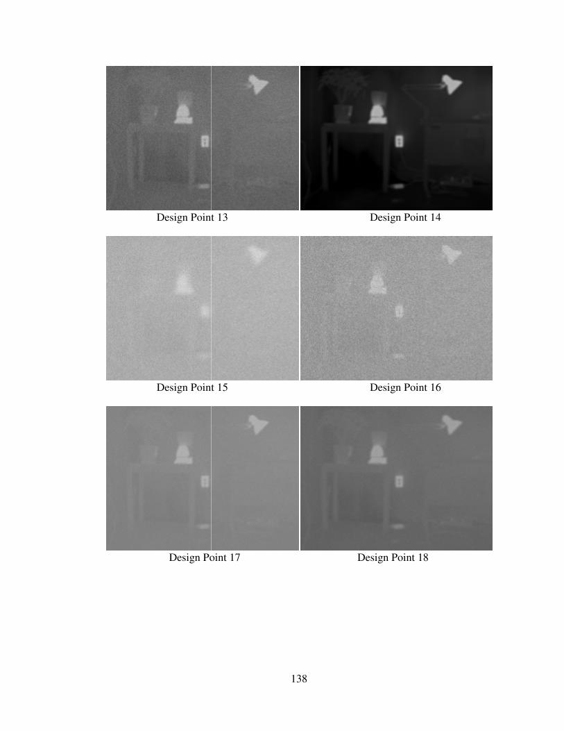
Design Point 13
Design Point 15
Design Point 17
138
Design Point 13 Design Point 14
Design Point 15 Design Point 16
Design Point 17 Design Point 18
Design Point 14
Design Point 16
Design Point 18
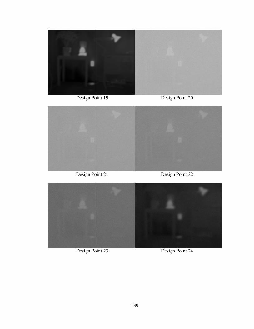
Design Point 19
Design Point 21
Design Point 23
139
Design Point 19 Design Point 20
Design Point 21 Design Point 22
Design Point 23 Design Point 24
Design Point 20
nt 22
Design Point 24

Design Point 25
140
Design Point 25

141
Bibliography
Agresti, A. (1990). Categorical Data Analysis. New York: John Wiley & Sons.
Amon, F.K.; Bryner, N.P.; Hamins, A., (2005) NIST Special Publication 1040
Amon, F. K.; Bryner, N. P.; Hamins, A. (2005) NIST SP 1040; NIST Special Publication
1040.Thermal Imaging Research Needs for First Responders: Workshop Proceedings.
December 9-10, 2004, Gaithersburg, MD, 70 pp, 2005.
Amon, F.K,Bryner, N.P., Hamins, A., Lock, A., (2008) NIST Technical Note 1499
Amon, F.K, Lock, A.; Bryner, N.P.; “Suite of proposed Imaging Performance Metrics
and Test Methods for Fire Service Thermal Imaging Cameras.”National Institute of
Standards and Technology.
Bracewell, R.N. (1989). “The Fourier Transform”. Scientific American, June 1989
Boreman, G.D. (2001). Modulation Transfer Function in Optical and ElecroOptical
Systems., SPIE – The International Society for Optical Engineers, Bellingham, W.A.
Cooley, J.W. and Tukey, J.W. (1965). An Algorithm for the machine calculation of
complex Fourier series. Mathematics of Computation.
Dobson, A.J. (1990) An Introduction to Generalize Linear Models, Great Britain: TJ
Press Ltd.
Grosshandler, W. L. (1993) “RADCAL: A Narrow-Band Model for Radiation
Calculations in a Combustion Environment, NIST Technical Note 1402.” National
Institute of Standards and Technology.
Holst, G.C. (1998). Testing and Evaluation of Infrared Imaging Systems., SPIE Optical
Engineering Press and JCD Publishing, Winter Park, FL.
Holst, G. C. (2000). Common Sense Approach to Thermal Imaging., SPIE Press and JCD
Publishing, Winter Park, FL.
Kruse, P.W. (1997). “Principles of Uncooled Infrared Focal Plane Arrays.” In: Uncooled
Infrared Imaging Arrays and Systems, P.W. Kruse, and D.D. Skatrud, eds., Academic
Press, San Diego.
ISO 12233, (2000). “Photography – Electronic still-picture cameras-Resolution
measurements,” International Standards Organization, Geneva, Switzerland

142
Lehar, S. An Intuitive Explanation of Fourier Theory
Lloyd, J.M. (1979). “Thermal Imaging Systems.” Plenum, New York.
Muralt, P. (2001). “Micromachined infrared detectors based on pyroelectric thin films.”
Reports on Progress in Physics, 64(10), 1339-1388.
Neter, J., Kutner, M., Nachtsheim, C., & Wasserman, W. (1996). Applied Linear
Statistics Models, Fourth Edition. Boston: McGraw-Hill
NFPA 1801, (2008). “Proposed NFPA 1801 Standard on Thermal Imagers for the Fire
Service, 2009 Edition”, National Fire Protection Association
Russ, J.C. (2002) The Image Processing Handbook Fourth Edition. CRC Press, Boca
Raton, Florida
Sanchez, S.M. (2007) Work Smarter, Not Harder: Guidelines for Designing Simulation
Experiments, Operations Research Department and Graduate School of Business &
Public Policy Naval Postgraduate School, Montery, CA
Smith, S.W. (2007) The Science and Engineering Guide to Digital Signal Processing,
California Technical, California
Theory of Thermography (2007). FLIR Systems User’s Manual 249-258
Tsai, C. F., and Young, M. S. (2003). “Pyroelectric infrared sensor-based thermometer
for monitoring indoor objects.” Review of Scientific Instruments, 72(12), 5267-5273
Video Electronics Standards Association Display Metrology Committee (2001). “Flat
Panel Display Measurements Standard Version 2.0”.
Weeks, A.R. (1996). Fundamentals of Electronic Image Processing., SPIE – The
International Society for Optical Engineers, Bellingham, WA.


![arXiv:2003.04857v1 [cs.CV] 10 Mar 2020 · Under-Display Camera 1 Introduction Under-display Camera (UDC) is a new imaging system that mounts display screen on top of a traditional](https://static.fdocuments.in/doc/165x107/5f4c26b7b44c764d7a4d605f/arxiv200304857v1-cscv-10-mar-2020-under-display-camera-1-introduction-under-display.jpg)