Policy Research Working Paper 8434

The Impact of Positive Agricultural Income Shocks on Rural Chinese Households

Jessica Leight

Development Economics Vice PresidencyStrategy and Operations TeamApril 2018

WPS8434P

ublic

Dis

clos

ure

Aut

horiz

edP

ublic

Dis

clos

ure

Aut

horiz

edP

ublic

Dis

clos

ure

Aut

horiz

edP

ublic

Dis

clos

ure

Aut

horiz

ed

Produced by the Research Support Team

Abstract

The Policy Research Working Paper Series disseminates the findings of work in progress to encourage the exchange of ideas about development issues. An objective of the series is to get the findings out quickly, even if the presentations are less than fully polished. The papers carry the names of the authors and should be cited accordingly. The findings, interpretations, and conclusions expressed in this paper are entirely those of the authors. They do not necessarily represent the views of the International Bank for Reconstruction and Development/World Bank and its affiliated organizations, or those of the Executive Directors of the World Bank or the governments they represent.

Policy Research Working Paper 8434

This paper is a product of the Strategy and Operations Team, Development Economics Vice Presidency. It is part of a larger effort by the World Bank to provide open access to its research and make a contribution to development policy discussions around the world. Policy Research Working Papers are also posted on the Web at http://www.worldbank.org/research. The author may be contacted at eight@american.edu.

In the post-collectivization period, rural Chinese house-holds were required to sell part of their grain output to the state at a below-market price; however, increases in this quota price beginning in 1993 generated substantial positive income shocks. These income shocks also varied cross-sectionally in accordance with crop composition given that quotas were systematically larger for rice-pro-ducing households, generating a quasi-random source of variation in the size of the shock driven by climatic varia-tion in suitability for rice cultivation. Households induced

to experience relatively larger income shocks show evi-dence of decreased agricultural investment, increased investment in non-agricultural businesses, and increased migration as households gain increased income, consis-tent with the hypothesis that credit constraints may have constrained some households from entering non-agricul-tural production ex ante. In addition, there is evidence that these households were concentrated among house-holds who had not previously diversified out of agriculture.

The impact of positive agricultural income shocks onrural Chinese households∗

Jessica Leight

∗Jessica Leight (corresponding author) is a professor at American University, Washington, D.C.,U.S.; her email address is leight@american.edu. The author thanks Abhijit Banerjee, Loren Brandt,Esther Duflo, William Gentry, Doug Gollin, Rohini Pande, Albert Park, and Xiaobo Zhang for detailedfeedback and seminar participants at the MIT political economy breakfast, Williams, Cornell, IFPRI,Beijing University, the Chinese Center for Agricultural Policy, and the Hong Kong University of Scienceand Technology for comments.

1 Introduction

A large literature in development economics has sought to analyze the effects of both

positive and negative income shocks on poor households, and in particular to probe

whether such shocks lead to any systematic shifts in the allocation of productive activities.

In China, rural households in the post-1983 period were required to sell a fixed quota of

grain to the state at a below-market price as part of the so-called Household Responsibility

System implemented following decollectivization. However, the central government began

to raise this price gradually in the mid-1990s (Huang and Rozelle, 2002). This shift was

equivalent to a reduction in the size of the lump-sum tax imposed on rural households

(Huang, 1998), or conversely, a positive income shock; moreover, given that grain quota

prices remained high thereafter, the shock was plausibly viewed as an increase in both

current and future expected income.

This paper estimates the impact of this policy-driven shock on investment in agricul-

tural and non-agricultural production, seeking to identify whether a lump-sum increase

in income leads to a reallocation of productive activities. Crucially, the size of this shock

varied systematically as a function of the crop cultivated, given the stark difference in the

treatment of different crops under the quota system (Huang, Rozelle, Ha and Li, 2002).

Predominantly rice-growing areas systematically experienced larger income shocks, given

that they were subject to larger mandatory quota quantities than predominantly wheat-

growing areas. The identification strategy here exploits this cross-sectional variation in

conjunction with shocks to the quota price over time. While cultivation of rice is an

endogenous household decision, the specification of interest analyzes the impact of in-

creasing quota income for areas that have a greater propensity to cultivate rice based on

their climatic conditions, conditional on village and province-year fixed effects.

The results suggest that in an instrumental variables specification in which income

is predicted by the interaction of the propensity to cultivate rice and quota price, an

increase in quota income leads to a decrease in agricultural investment and an increase in

1

non-agricultural investment and migration. Households experiencing increases in quota

income also show evidence of a higher probability of accessing a non-zero amount of credit,

and increased consumption of non-staple goods. While the results should be interpreted

cautiously, the observed pattern is consistent with the hypothesis that credit constraints

may have been binding ex ante for some households, limiting their diversification into

non-agricultural productive activities. The positive income shock generated by the quota

price increase relaxes this constraint.

The results are also robust to a series of specification checks. The effects of the

quota shocks are observed primarily for households that have not diversified into non-

agricultural production ex ante, i.e., those that are plausibly constrained. There is no

evidence that these patterns reflect differential trends in areas with different climatic

conditions, or differential shocks in policy or other output prices correlated with the

quota price. There is also little evidence that variations in quota policy are endogenously

driven by varying conditions in the local economy.

This paper contributes to several related literatures. First, a large literature has

analyzed the effects of income shocks, both negative and positive, on developing coun-

try households’ pattern of asset-holdings and livelihood diversification. A number of

papers provide evidence that households facing negative shocks derived from adverse

weather outcomes or natural disasters experience asset disinvestment as well as con-

sumption declines, and these effects are particularly salient for poor households (Carter,

Little, Mogues and Negatu, 2007; Carter and Lybbert, 2002; Janzen and Carter, 2013;

Hoddinott, 2006). In analyzing positive shocks, by contrast, Barrett et al. (2001) evalu-

ate the effects of exchange rate and food aid shocks on household diversification in Cote

d’Ivoire and Kenya. Gertler, Martinez and Rubio-Codina (2012) and Sadoulet, de Janvry

and Davis (2001) find that households benefiting from cash transfer programs in Mexico

invest transfers in productive assets, resulting in a long-term increase in consumption;

Gilligan, Hoddinott and Taffesse (2008) find similar results examining a government assis-

tance program in Ethiopia. Blattman, Fiala and Martinez (2014) find that cash transfers

2

to young adults for non-agricultural activities lead to increases in assets and income.1

Second, a number of papers have analyzed how households respond to evolution in

the rate of return on agricultural investments. Foster and Rosenzweig (2004) estimate

the impact of shocks to the returns to agriculture in India induced by the adoption of

Green Revolution technology and find that industrial growth is fastest in areas where

agricultural growth is lagging. Jedwab (2011) finds that positive price shocks to cocoa

during cocoa booms in Ghana and the Ivory Coast lead to an increase in urbanization.

Kaboski and Townsend (2011) evaluate the impact of a government-sponsored microcredit

program as a major income shock in rural Thailand on consumption and investment.

Most recently, Bustos et al. (2016) present evidence that the introduction of genetically

engineered soybean seeds in Brazil leads to industrial growth.

Third, this paper contributes to the body of work focused on analyzing the grain

quota system as it operated in China. Lu (1999) describes broad trends in the operation

of the quota system over time, and Rozelle et al. (2000) describe reform over the decade

of the 1990s, particularly the backlash following early attempts at liberalization. Huang,

Rozelle and Wang (2006) evaluate the quota system as part of a broader analysis of

capital flows in and out of the agricultural sector. Further discussion of existing work

describing the grain quota system can be found in Section 2.2.

More recently, a broader literature in macroeconomics has documented large gaps in

labor productivity between the agricultural and non-agricultural sectors in developing

countries, and relatedly, a large gap in labor productivity comparing the agricultural

sector in developing and developed countries (Gollin, Lagakos and Waugh, 2014; Lagakos

and Waugh, 2013). While this paper does not directly analyze productivity gaps across

sectors, the suggestive evidence of constraints on exit from agriculture is consistent with

1While this empirical analysis does not directly address the question of poverty dynamics in ruralhouseholds, and focuses instead on dynamics in sectoral allocation over time, there is also a large literatureanalyzing the presence or absence of poverty traps in developing country contexts. Kraay and McKenzie(2014) provide a useful overview. In particular, it may be useful to highlight that the evidence of steadilyincreasing income and substantial sectoral mobility for rural households in China renders this contextdistinct from many other developing countries, particularly in sub-Saharan Africa, where there is moreevidence of income stagnation and/or structural immobility (Giesbert and Schindler, 2012; Kwak andSmith, 2013; Naschold, 2012, 2013; Quisumbing and Baulch, 2013).

3

the presence of a large and relatively unproductive agricultural sector.

Relative to the existing literature, this paper provides new evidence about the effect

of a quasi-exogenous income shock on productive diversification for rural households, and

has the advantage of exploiting a plausibly permanent income shock. It is also one of the

first papers to analyze the impact of variation in quota policy in China on investment in

non-agricultural production. The paper proceeds as follows. Section 2 describes the data

and institutional background, and Section 3 presents the identification strategy. Section

4 presents results and robustness checks, and Section 5 concludes.

2 Data and institutional background

This section briefly summarizes the data employed, provides an institutional overview of

the grain quota system, and describes the information available in the dataset about the

quota system.

2.1 Overview of data sources

The data employed here is the China Research Center for the Rural Economy panel

dataset, collected in a sample of 206 villages in 13 provinces in China between 1986

and 2001, excluding 1992 and 1994.2 Provinces observed include Shanxi, Jilin, Jiangsu,

Zhejiang, Anhui, Henan, Hunan, Sichuan and Gansu. The surveys prior to 1993 were

considerably briefer, and thus the primary analysis is restricted to the post-1993 panel;

1993 is identified as the baseline year.

In addition, the analysis employs two climatic or agronomic data sets. The first is

monthly climatic data from a network of weather stations in China collected by the

Carbon Dioxide Information Analysis Center (CDIAC). Using data on the latitude and

longitude of the county centroid, climatic measurements for each county and year are

2A randomly selected sample of households in each surveyed village forms the panel; the mean numberof households in a village-year cell is 69.

4

constructed by interpolating using the inverse distance weighting method.3 The second

is an index of climatic suitability for rice cultivation generated by the FAO, incorporat-

ing precipitation and temperature as well as other soil and topographic features. More

specifically, the analysis utilizes the FAO’s index of suitability for high input-level irri-

gated rice, given that Chinese agriculture is characterized by a relatively high level of

input use and irrigation, and estimate the mean index value within the county in which

each sampled village lies (IIASA and FAO, 2012). More details on how these indices are

used in the analysis are provided in Section 3.

2.2 Grain policy in China

Prior to 1978, agricultural production in China was highly collectivized. The primary

unit of production was the production team, a cluster of 20 to 30 households that jointly

farmed agricultural land and sold the resulting output. After the death of Mao Ze-

dong, however, major changes in agricultural policy were introduced. The household was

reinstated as the primary unit of production under a system known as the Household

Responsibility System. Each household was provided with an allocation of land for its

own use, while land title continued to be held by the village (Brandt et al., 2002).

In addition, households were mandated to deliver a fixed amount of quota grain to

the state at a preset price. Excess production could be sold to the state at a higher,

above-quota price, or at rural markets (Lin, 1992). Grain thus sold to the state was

primarily funneled via official grain bureaus to urban consumers, who were entitled to

purchase staple consumption goods at subsidized prices (Lu, 1999; Rozelle et al., 2000).

This mandatory grain procurement by the state, widely known as the grain quota

system, remained a key dimension of agricultural policy through the early post-2000

period. The volume of grain quotas did decline after 1995 relative to earlier in the

3Each interpolation employs only data from stations within 150 kilometers of the county centroid.The average number of stations employed to construct climatic data for a county is three. While county-level weather data reported directly by counties to provincial weather bureaus is also available, usingweather station data has the advantage of ensuring consistency of data quality and reporting methodsacross the sample.

5

decade; subsequent surveys have found that state procurement accounts for 25–30% of

rural households’ grain output, though in this sample, quota sales constitute only around

10% of grain production on average (Wang et al., 2003; Sicular, 1995).4

More importantly, there was a substantial increase in quota prices beginning in 1993.

The primary analysis in this paper will focus on the period 1993 to 2002; evidence in

this sample suggests that at the beginning of the period, the quota price was 30% lower

than the market price. In some years later in the period, however, the prices were nearly

equal. This change is equivalent to a large reduction in the magnitude of the lump-sum

tax imposed on farmers via the mandatory quota system (Huang, 1998). More recently,

grain quotas have been widely eliminated. The timing of this change varied, but generally

occurred post–2002, after the period of interest here (Huang, Wu and Rozelle, 2009).

It is also useful to note that the quota system treated different grain crops very dif-

ferently, and rice was consistently the crop most heavily penalized. Procurement prices

for rice were lower, and rose more slowly. In addition, the quota quantity constituted a

higher proportion of total production for rice producers than for wheat producers (Huang,

Rozelle, Ha and Li, 2002). The identification strategy in this paper will exploit the sys-

tematic cross-sectional variation in quota quantity that is correlated with cross-sectional

variation in the propensity to cultivate rice, in conjunction with these fluctuations in the

quota price over time, in order to identify variation in quota income.

In terms of the implementation of the quota system, Wang et al. (2003) provide a de-

tailed analysis of the system’s operation during the period examined here. Quota prices

were set by the central government and were constant at the national or provincial level,

while quota quantities in the form of grain deliverable per household were generally set

4Sicular (1995) reports aggregate statistics on the percentage of farm output sold as quota salesbetween around 1985 and 1993; grain quotas fall rapidly in this period, accounting for the fact that thepercentage of total output constituted by the quota in this sample, observed between 1993 and 2002,is lower. Wang et al. (2003) report data on the operation of the grain quota system assembled fromsecondary data sources (i.e., not household surveys) in 25 counties in Zhejiang, Jiangsu and Sichuan forthe years 1980 to 1999. They report that the share of the quota in total output is less than 25% after1995. Given that two of the three provinces included in the survey are relatively high-income, high-productivity provinces, the fact that quota sales constitute a relatively higher percentage of output maybe unsurprising; there is in general a positive correlation between the level of agricultural productionand the proportion of total output sold as quota sales.

6

by county leaders for all villages within their jurisdiction, and varied with village charac-

teristics. Wealthier, more productive, and more agricultural villages were assigned higher

quotas. Given that these analyses employ secondary data that report county- or village-

level averages for quota quantity, there is no analysis of intra-village variation in quota

quantity. Furthermore, quota quantities for a given village changed only incrementally

once set by county leaders. By contrast, the central government had discretion over the

grain quota price and would change it annually (Rozelle et al., 2000; Lin, 1991).

2.3 Descriptive statistics around quota income

This section provides an overview of the quota and market price over time, and describes

the key sources of variation in the quota price.

Quota and market price over time The RCRE household data used in this analysis

provides information on the price for both mandatory grain quota sales and market sales,

as well as the volume of grain quota sales at the household level.5 Figures 1a and 1b

report the mean market and quota price of grain by year between 1986 and 2002, and

additionally capture spatial variation in prices, showing in each year the 5th and 95th

percentile of the within-year, cross-village distribution of prices; Figure 1a shows the

cross-village variation in market prices, and Figure 1b shows the cross-village variation

in quota prices.6 Prior to 1991, both prices are low and stable. The market price begins

to dramatically increase after 1991, and the quota price likewise increases, though more

slowly. Cross-village variation in quota price is relatively limited, while the cross-village

5After they have fulfilled their grain quota, rural households also have the option to sell their excessproduction to the government at a higher, negotiated procurement price. Huang, Rozelle, Ha and Li(2002) show that these negotiated procurement prices are generally intermediate between the quota priceand the wholesale market price. In this data, negotiated procurement prices are not reported, and nodistinction is made between these two types of sales, as both represent the price that the rural producerwould face for the marginal unit of production. The market price is thus used to denote the price formarginal grain sales.

6Price data is constructed at the household level for households that report market or quota sales,but a large number of observations are missing, corresponding to cases in which households do not reportmarket sales in particular year. Accordingly, price data is collapsed to the village-year level, as everycell has sufficient data to estimate a market price and a quota price. Observations corresponding to thetop and bottom 1% of observed prices across villages are trimmed to avoid undue influence of outliers.

7

variation in market price is more substantial.

Figure 1c shows mean income from quota sales at the household level (reported in

hundreds of yuan) by year, again reporting the 5th and 95th percentile; the 5th percentile

is uniformly zero, corresponding to households that report no quota sales. In addition,

it is useful to estimate the magnitude of the implicit quota tax, defined as the difference

between the market and quota price multiplied by the quota quantity, as a percentage

of total income. The evolution of the quota tax is summarized in Figure 1d; it peaks in

1995, at around 5% of income, and is lowest in 1998 and 1999, where it is nearly zero for

all households.

In order to highlight the difference between the cross-household and cross-village

distributions, Figures S1a and S1b in the appendix reproduce these figures, but also

add the corresponding 5th and 95th percentiles of the within-year distribution of village-

level means of the quota income and the quota tax. (It is evident that the majority

of the variation is cross-village, rather than cross-household and within-village. This is

consistent with the evidence from the literature that the primary determinants of quota

policy vary at the village level.

Focusing on the quota tax, there is clearly considerable variation in the implicit tax

rate posed by the quota, with some households reporting rates of up to 10%, or even higher

in 1995. In addition, this tax rate is systematically higher for lower-income households;

given that there is relatively little within-village variation in quota quantity, the quota

tax is regressive. More specifically, the implicit tax posed by the quota system is always

close to zero for households in the top quantile of income, but it averages 2% of income

for households outside the top income quantile, and 5% of income for households outside

the top income quantile prior to 1996.7

7Previous papers in the literature have analyzed shocks that varied in size. Gilligan et al. (2008) intheir analysis of an Ethiopian safety net program do not provide an estimate of the transfer’s size relativeto income, bur rather focus on measures of caloric intake. Blattman et al. (2014) analyze a much largershock in northern Uganda, equal to approximately 100% of the participants’ annual income; however,this paper also reports much larger effects than will be observed here. Barrett et al. (2001) analyzed afood-for-work program implemented in Kenya that provided wages equal to approximately 15% of annualincome, and Gertler et al. (2012) analyze transfers provided by Progresa, for which there is substantialvariation in the relative size of the payment depending on household structure. In general, the shock

8

Finally, it is useful to highlight while the market price is fluctuating during this period,

it is primarily shifts in the quota price that serve to close the gap between the two prices.

In particular, the quota price is consistently below the market price in the early part of

the period, but it converges upward to the market price after 1996. This convergence

generates a positive income shock that is also plausibly expected to be permanent, given

that quota prices subsequently remain high.

Defining an alternative quota price measure P̃ The graphical evidence presented

here clearly suggests that some of the variation in the quota price is driven by variation in

the market price; more specifically, the quota price can be described as a linear function

of the market price, α+βPm+ε. The parameters α and β reflect the average relationship

between the market and quota price over time, and in general Pq < Pm.

Given that shifts in the market price can have many other complex effects, however,

this analysis will not exploit variation in the quota price that reflects underlying fluctua-

tions in the market price. Rather, the primary objective is to exploit variation in quota

policy in which the government sets a quota price that is abnormally high (or low) rela-

tive to the market price — that is, increases (decreases) in the quota price conditional

on the market price. A high quota price shock is characterized as a positive ε, resulting

in the quota price exceeding the predicted quota price based on prevailing market prices.

There will correspondingly be years in which the quota price is lower than the predicted

quota price based on prevailing market prices, and ε is negative.

In order to generate estimates of these shocks, the mean quota price in each village

v in province p in year t is regressed on the corresponding market price in the following

equation, conditional on village fixed effects λvp.

P qvpt = βPm

vpt + λvp + εvpt (1)

The residual from this equation is then constructed, denoted P̃vpt. By construction,

analyzed here is somewhat smaller in magnitude, but also differs in that it was plausibly permanent.

9

the residual is uncorrelated with the market price, and all subsequent analysis of the

quota price will employ this variable P̃vpt. Further specifications presented in Section

4.1 demonstrate that the primary results are robust to re-defining the quota price. The

hypothesis that fluctuations in P̃vpt may be correlated with other observable covariates is

explored further in the appendix.8

Variation in quota quantity and price across time and space In the primary

analysis, the quota price variable P̃vpt will be interacted with a cross-sectional climatic

index and employed as an instrument for quota income, defined as the income received by

households from their grain quota sales. The empirical strategy seeks to exploit variation

across villages in quota quantity and variation over time in quota price given that the

institutional background suggests these are the primary dimensions of variation for each

variable. However, this hypothesis can also be confirmed in the data.

If quota quantity is regressed on village fixed effects and year fixed effects, village

fixed effects account for around 35% of the variation in quota quantity, while year fixed

effects account for only 7% of variation. If household fixed effects are included instead of

village fixed effects, the R-squared increases to 67%.9 For the quota price, the pattern is

inverted. If the quota price variable is regressed on year fixed effects, the R-squared is

around 50%; if year fixed effects are replaced by province-year fixed effects, the R-squared

again increases to 70%.

Accordingly, quota income is decomposed as the product of a quota price P̃ that is

time-varying but does not systematically vary by village, and a quota quantity Q that

varies across localities (and to a limited extent within them), but is approximately con-

stant over time. Importantly, quota quantity not only varies across localities, but varies

systematically, and will generally be higher for richer and more agriculturally productive

8These results can be found in Section S6.2.9This is consistent with the hypothesis that there is some within-village variation in quota quantity,

in addition to the cross-village variation discussed in Wang et al. (2003). Again, previous analyses ofquota quantity have primarily employed secondary data reported at the village or county level, and thushave been unable to analyze within-village variation in quotas.

10

villages; this comparative static will also be confirmed in the data.

3 Identification strategy

This section first identifies the key identifying variation in quota quantity that will be

exploited, and then reports the first stage.

3.1 Endogeneity of quota quantity

As already noted, quota quantity is endogenous, correlated with many observable and

unobservable local characteristics. My objective here is to identify a time-invariant,

cross-sectional variable correlated with quota quantity and interact it with the price in

order to generate an instrument for quota income. Given the widespread analysis in

the literature of the systematic cross-sectional differences in quota policy implementation

that correspond to variation in crop composition, variation in the propensity to cultivate

rice will be the key source of variation this analysis will exploit.

To demonstrate the robustness of this relationship and increase precision in the pri-

mary two-stage least squares results, the analysis will utilize two different variables cap-

turing the propensity to cultivate rice based on agronomic and climatic conditions. The

first measure is constructed directly from climatic data (referred to thereafter as the “cli-

matic index”); the second measure is drawn from an index generated by the Food and

Agriculture Organization (referred to as the “FAO index”).

First, in China, as in other countries, the suitability of a region for rice cultivation is

partially determined by temperature and precipitation. “Total temperature” is defined

as the total accumulated temperature over a year for days with temperatures above 10

degrees Celsius; the agronomic literature suggests the total temperature must exceed 2000

degrees to cultivate rice in China (Shao et al., 2001). Similarly, “seasonal precipitation”

is defined as mean precipitation observed between May and October, the key cultivation

months for rice (Tang et al., 2010). For both variables, the mean total temperature or

11

seasonal precipitation observed in each county over the period of interest is calculatde

to generate a time-invariant climatic variable. The climatic index is constructed as the

mean of both variables, and denote this index Climvp for village v in province p.10

Second, the analysis utilizes a FAO-generated index of agronomic suitability for high-

input irrigated rice. This index is time-invariant, and is calculated for each sampled

locality as the mean value observed within the borders of the county in which the locality

lies, denoted FAOvp.

It is important to clarify the level at which both indices vary. The variables of interest

(Climvp and FAOvp) are constructed using the geographic coordinates reported for the

county in which each village lies, given that this is the lowest level at which linkable

geographic indicators are reported for this dataset; village-level geocoding information is

not publicly available. However, in this sample, cross-county heterogeneity is virtually

equivalent to cross-village heterogeneity, as only one village is sampled per county.11 The

underlying variation for the climatic index is drawn from geo-coded data reported by 730

weather stations across China. To take into account spatial correlation in climatic charac-

teristics, the standard errors in all subsequent specifications will be estimated employing

two-way clustering at the province and year level, to allow for arbitrary correlation in the

climatic index across observations in the same province.12

The relationship of interest between climatic conditions and quota quantity can be

estimated by regressing quota quantity on these climatic indices, conditional on province-

year fixed effects; in addition, the direct correlation between quota quantity and rice area

is estimated. Quota quantity for household i in village v, province p, and year t is denoted

Qivpt; area cultivated in rice is denoted Aivpt; and province-year fixed effects are denoted

10Precipitation is re-scaled to have the same mean as total temperature. The top and bottom 2% ofclimatic index observations are trimmed to minimize the effects of outliers.

11There are two pairs of villages located in the same county in the core sample.12More specifically, standard errors are estimated employing the ivreg2 command in Stata and the

two-way clustering option.

12

νpt. The equations of interest are thus written as follows:

Qivpt = βClimvp + νpt + εivpt (2)

Qivpt = βFAOvp + νpt + εivpt (3)

Qivpt = βAivpt + νpt + εivpt (4)

Columns (1) through (3) of Table 1 report the results, suggesting that a one standard

deviation increase in the propensity to cultivate rice increases the quota quantity by at

least 40% for localities within the same province and year.13 A one standard deviation

increase in rice area increases the quota quantity by 50%. This is an effect of substantial

magnitude, and it does not rely on the cross-provincial heterogeneity evident in China

between southern rice-cultivating and northern wheat-cultivating provinces.

3.2 First stage

Again, the objective of the identification strategy is to identify variation in quota quantity

that is correlated only with variation within a province in the propensity to cultivate

rice. This variation is then presumed to be uncorrelated with other economic or political

variables that enter into the county leader’s determination of quota quantity.

Accordingly, the two climatic indices are interacted with a time-varying measure of

quota price to generate instruments for quota income. Columns 4 and 5 of Table 1 report

the two specifications of interest, regressing quota income on the interaction of climatic

index and price conditional on village and province-year fixed effects. Standard errors are

estimated employing two-way clustering at the province and year level. The estimating

13It should be noted that the sample for these and all subsequent regressions is limited to household-year observations that report both quota quantity and climatic data. Less than 1% of household-yearobservations do not report the quantity of grain sold for the quota. About 13% of household-yearobservations are missing climatic data. This reflects villages located in counties for which only outdatedcounty codes are available, as the original county has since changed boundaries or dissolved; given thatit is not possible to ascertain in which successor county the village of interest lies, these localities havebeen dropped. There is no correlation between the probability a given village is missing climatic dataand the average quota quantity, quota price, or area reported cultivated in rice in that village.

13

equation is as follows, where Iivpt denotes quota income, and λvp and νpt are village and

province-year fixed effects, respectively; a parallel specification is estimated employing

the FAO index.

Iivpt = βClimvp × P̃vpt + λvp + νpt + Climvp × P sumivpt + ηclimvp × P g

ivp,t−1 + ηclimvp × γt

+ ηindvp × γt + εivpt (5)

The price variable employed is uncorrelated with the market price of grain by con-

struction, but controls are also included for the interaction of the climatic index and a

summary variable of other agricultural prices P sumivpt , and the interaction of dummy vari-

ables for quantiles of the overall climatic index ηclimvp with the lagged market price of

grain.14 Additional control variables include climate quantile fixed effects interacted with

year fixed effects and dummy variables corresponding to the quantiles of industrial em-

ployment in the village ηindvp interacted with year fixed effects to allow for varying trends

over time in areas of differing levels of industrialization.

The results indicate that a one standard deviation increase in the interacted instru-

ment leads to an increase in quota income of around 15%, and in both cases, the relation-

ship is precisely estimated and of comparable magnitude. The magnitude is calculated

by noting that a one standard deviation increase in the normalized instrument yields an

increase of approximately .3 in quota income measured in hundreds of yuan, relative to

a mean of 2.065.15 To reiterate, the exclusion restriction for these specifications requires

that an increase in the quota price has no differential impact across areas with varying

propensity to cultivate rice, other than a varying lump-sum income shock. The objective

is to capture the differential effect of an increase in the quota price on a locality where

the quota quantity is higher by virtue of its climatic suitability for rice cultivation.

Several assumptions are embodied in this specification. First, a shift in the quota price

14The summary price variable constructed is the mean of the market prices of the most commonagricultural products reported sold: rice, wheat, corn, soy, fruit, vegetables, and cotton.

15Unsurprisingly, the two instruments are highly correlated with each other (correlation coefficient of.88).

14

is assumed to represent an income shock, rather than a price shock. Second, the implicit

decomposition of quota income postulated is Q × P̃ , where Q is treated as time-fixed

and endogenous and P̃ as time-varying and exogenous. Third, it is assumed that shifts

in climate do not induce systematic changes in quota income other than those mediated

by changes in rice area cultivated. Fourth, it is assumed that yearly fluctuations in

climate are uncorrelated with shifts in the quota quantity. Evidence consistent with the

first assumption is presented here, as these results are essential to defining the primary

specification. Additional specification checks that suggest the secondary assumptions are

also valid are presented in Section S2 of the appendix.

There are two primary channels through which the assumption that a shift in the

quota price is an income effect rather than a price effect could be violated: substitution

in and out of agriculture, and substitution between crops.16 The first potential channel

is relevant if shifts in the quota price induce households to substitute in and out of

agriculture entirely. Households not cultivating grain are still required to provide grain

they have purchased or an equivalent cash payment (Brandt, Rozelle and Turner, 2004);

however, when they re-optimize their production decisions in the next year, the quota

price will be the price of the marginal unit of grain production. Complete exit from

grain cultivation is rare. Only 10% of households report even one year in which they

do not cultivate grain, and on average these households still report cultivation in about

half the years surveyed. For analytical clarity, however, all households that do not report

grain cultivation in every year have been dropped from the analysis. Importantly, the

probability that a household reports complete exit from grain cultivation is uncorrelated

with the propensity to cultivate rice, and thus, dropping these households does not create

differential patterns of selection into the sample in treatment and control areas.17

16The potential challenge of households for which quota production is equal to total production isdiscussed in the appendix.

17This strategy may pose a challenge for external validity, as the resulting estimates cannot be ex-trapolated to households for which exiting agriculture entirely is a meaningful counterfactual. However,given the extremely small number of households that show this pattern and the fact that a much morecommon empirical regularity – as will be elaborated further below – is households that simultaneouslypursue agricultural production, non-agricultural household production and/or employment outside thehousehold – this does not seem to be a major concern.

15

A second channel through which an income effect could be a price effect is if households

switch crops in response to changes in the quota price and begin selling a larger quantity

of rice as their mandated quota (rather than the smaller mandated quantity of wheat)

when the price increases. While this may not be optimal if the quota price remains below

the market price, as it does on average, it could be locally optimal if the quota price

is close to the market price in some village-years. In this case, if households have some

discretion over the quantity they sell, then a change in the quota price can no longer be

plausibly interpreted as a change in a lump-sum tax.

In order to test this hypothesis, villages are classified as heterogeneous or homoge-

neous in the primary grain crops of interest (rice or wheat) using a simple rule: any

village in which the total amount of both rice and wheat cultivated over all observations

exceeds zero are denoted as heterogeneous cultivators.18 The remaining villages (consti-

tuting approximately 60% of all observations) are classified as homogeneous cultivators.

Columns (6) and (7) of Table 1 show the results of estimating the following regression

to test whether quota quantity varies year-on-year with changes in quota price. This

equation is estimated for both homogeneous and heterogeneous villages, denoted “Hom”

and “Het,” respectively.

Qivpt = βP̃vpt + λvp + εivpt (6)

The results show that the relationship in homogeneous villages is close to zero and

insignificant, while the coefficient in heterogeneous villages is positive and significant.

This suggests either that households are crop-switching or there are other inconsistencies

in quota implementation in heterogeneous areas. For example, some households in het-

erogeneous production areas may be opting to produce a crop other than rice to avoid

the high rice quota. If this choice is costly, when the quota price increases, households

may opt to return to rice production.

Accordingly, the primary sample will be restricted to villages that are homogeneous

in grain production of rice or wheat; in these villages, there is no evidence that quota

18Observations reporting cultivation of less than .01 hectare rounded down to zero.

16

quantity is endogenously determined by the price. The specifications of interest reporting

the first stage in the restricted sample of homogeneous villages are presented in Columns

(8) and (9) of Table 1, and suggest a one standard deviation increase in the interacted

instrument leads to an increase in quota income of around 10%. The exclusion restriction

for this analysis requires that fluctuations in quota price are not correlated with any

other shocks that vary systematically across areas with varying propensity to cultivate

rice based on their climatic conditions. In other words, the only channel through which

an increase in the quota price differentially affects areas more and less likely to cultivate

rice is via the differential impact of a quota price increase on quota income.

4 Results

First, it is useful to briefly characterize the primary sample using the summary statistics

provided in Table 2. The average household consists of four individuals, cultivating

an area of around 1.4 hectares primarily in grain.19 90% of household-year observations

report ownership of at least one productive asset for use in agriculture (e.g., animals, tools

or machinery). 26% of household-year observations report ownership of non-agricultural

capital, and about 40% report that at least one household member is engaged in wage

labor outside the household.

The analysis will focus on the effect of increased quota income on investment in and

income derived from agriculture, investment in and income derived from non-agricultural

household businesses, outside employment, migration, borrowing, and consumption. For

two outcomes of interest – investment in agriculture, and investment in non-agricultural

businesses – the results are reported employing a summary variable constructed using

principal-component analysis, standardized to have mean zero and standard deviation

one, as well as disaggregated results for a number of separate variables. Additional details

about variable construction, particularly for agricultural income and consumption, are

19In China, mu is the traditional unit employed for land area; 1.4 hectares is equal to 21 mu.

17

reported in Section S1 of the appendix.

For agricultural investment, a summary variable is reported constructed employing

six variables: area sown, labor invested in days, value of fertilizer employed, value of seeds

employed, investment in animals, and investment in tools. Fertilizer, seeds and agricul-

tural investment are reported as expenditure in yuan, and deflated using a summary

price index for agricultural inputs published by the China National Bureau of Statistics.

Principal-component analysis is conducted on these six variables, and the first component

is employed as the summary index.

Agricultural income is calculated valuing all agricultural production (including live-

stock, fish, and forestry products) at the market price observed in each village-year cell;

the market price of each crop or product is calculated as a sales-weighted average of unit

prices reported by households. This income measure is then deflated using a weighted

Laspeyres price index constructed from the same prices, employing 1993 as the base year.

(Note this calculation abstracts from any variation introduced by quota policy itself, as

all production is valued at the market price rather than the quota price.)

To analyze non-agricultural production, results are again reported for variables captur-

ing non-agricultural investment and income. For non-agricultural investment, a summary

outcome measure is constructed using four variables: a dummy variable equal to one if

the household reports any new cash investment in a non-agricultural business, a dummy

variable equal to one if the household reports any labor invested in non-agricultural

machinery, and the amount of labor and cash investment reported in non-agricultural

businesses. It is important to note that both agricultural and non-agricultural invest-

ment as constructed here are flow measures: they capture new investments in the year

of interest. Again, the summary index is constructed via principal component analysis,

retaining the first component as the index of interest. Non-agricultural income is the sum

of income from non-agricultural household businesses and wage labor.

In order to deflate non-agricultural investment and income to constant prices, an index

of ex-factory prices for industrial products published by the National Bureau of Statistics

18

is employed. Unfortunately, the RCRE panel itself does not report disaggregated sales

for any non-agricultural product, and accordingly it is not possible to construct a price

index for non-agricultural inputs or outputs. The use of an index of factory prices may

not be ideal in the analysis of household-level businesses that may produce very different

products; this point will be addressed further in the discussion of the results below.

In addition, total income is constructed equal to the sum of agricultural and non-

agricultural income. Additional analysis reports a dummy variable for outside labor equal

to one if the household reports any days worked outside the household and associated

wage income; and a dummy variable for migration equal to one if the household reports

days worked outside the township. For borrowing, a dummy variable equal to one if

the household reports any access to credit (formal or informal) is utilized, as well as a

continuous variable equal to the amount borrowed.

Finally, results are reported for consumption of grain staples, non-grain consumption,

and total consumption. Grain consumption is the sum of expenditure on grain and the

imputed value of own-grain consumption, while non-staple consumption is the sum of

expenditure on all consumption items excluding staple grains (both food and non-food),

and the imputed value of consumption of own-farm non-grain products. Consumption

expenditure is deflated employing a province- and year-specific consumer price index

generated by Brandt and Holz (2006).

4.1 Two-stage least squares

The specification of interest can be written as follows, where Yivpt denotes economic

outcomes of interest and the primary independent variable is Iivp,t−1, lagged income from

grain quota sales. Standard errors are estimated employing two-way clustering at the

province and year level.

Yivpt = βIivp,t−1 + λvp + νpt + Climvp × P sumvpt + ηclimvp × P g

ivp,t−2 + ηclimvp × γt

+ ηindvp × γt + εivpt (7)

19

Again, the specification includes village and province-year fixed effects, the interaction

of industrial employment quantile dummies and year fixed effects, and the interaction of

climatic index quantile dummies and year fixed effects.20 Additional controls include the

interaction of the climatic index and the summary agricultural price variable, measured

contemporaneously, and the interaction of quantiles of the climatic index and the lagged

grain market price; as the market price of grain is lagged relative to the quota price, this

is a two-year lag relative to the outcomes of interest.

The results from estimating (16) are reported in Table S2, employing two instruments

for lagged quota income (the interaction of the climatic index and the quota price and

the interaction of the FAO index and the quota price); summary variables are reported

in Panels A and B, followed by disaggregated variables in Panels C and D, and all of the

dependent variables other than the dummy variables are standardized to have mean zero

and standard deviation one. (The ordinary least squares results are discussed in Section

S3 of the appendix.) For each specification in Table S2, the J statistic corresponding to

the Hansen test of overidentifying restrictions is reported. This test uniformly fails to

reject for the primary outcome variables.21

In Columns (1) and (2) of Panel A, we observe that the estimated coefficients for

agricultural investment and income are negative and significant: in other words, the

marginal complier household, induced to experience a larger increase in quota income

because of the climatic suitability of its land for rice, actually invests less in agriculture.

A 100-yuan increase in quota income in the prior year leads to a decline of around .2

standard deviations in agricultural inputs, and .1 standard deviations in agricultural

income. Disaggregated results for agricultural inputs reported in Panel C show a decline

in sown area of 15% that is not statistically significant, a 10% decline in labor, and a

20The fixed effects included are defined with respect to quantiles of the climate index constructedemploying temperature and rainfall; subsequent robustness checks will demonstrate that the primaryresults are robust to the addition of fixed effects defined using quantiles of the FAO index. The quantilesof the climatic index are identified within the subsample of homogeneous rice- or wheat-cultivatingvillages included in the analysis.

21The Kleibergen-Paap F statistic for the first stage is 5.4. The test of overidentifying restrictions failsfor one of the disaggregated variables: animal investment, as reported in Column (5) of Panel C.

20

large (more than 50%) decline in the value of seeds employed. There is no evidence of

significant shifts in the value of tools or animals.

By contrast, Column (3) of Panel A of Table S2 reports a positive effect of a quota

income shock on non-agricultural investment of around .2 standard deviations. The

disaggregated results in Panel D show increases in labor and cash investment in non-

agricultural businesses that are noisily estimated, and a significant increase in the prob-

ability of investing capital or labor in non-agricultural production. This suggests that

households are more likely to be establishing new non-agricultural businesses than ex-

panding existing businesses. There is no significant increase in non-agricultural income

(including income from non-agricultural businesses and wage labor), as reported in Col-

umn (4). If the same specification is estimated for income from non-agricultural busi-

nesses, however, there is a significant increase in income from this source of around .1

standard deviations. Given the differential effects for agricultural and non-agricultural

income, no significant effect is observed for total income, as reported in Column (5).22

In Column (6), we observe that there is no significant shift in the probability of en-

gaging in outside labor, though the coefficient of interest is positive. (The disaggregated

results in Panel D, Column (5) report the coefficient for the number of days worked outside

the household as a continuous variable, and again the estimated coefficient is insignifi-

cant.) There is, however, a significant increase in the probability of migration observed

in Column (7), suggesting that the positive income shock may also allow households to

fund migration costs.23

Finally, Panel B of the same table reports the results for credit access and consump-

tion. In Columns (1) and (2), we observe a significant increase in the probability of

22It is also useful to briefly return to the deflation of non-agricultural investment and income employingan index of ex farm prices. Given that the significant effects here are primarily observed for the dummyvariables for investment of cash or labor in a non-agricultural business, rather than the level of investment,the deflation of the level measures may not be of first-order importance. The reported results are alsoconsistent if the level measures are deflated using a consumer price index reported by Brandt and Holz(2006) — an approach that may be unsatisfactory given that this index also incorporates prices ofagricultural products — or if nominal values are employed.

23The mean value of the outside labor dummy is .40, and the mean value of the migration dummy is.20.

21

accessing credit of 10 percentage points on a base probability of around 20%, as well as

a significant increase in the amount of credit in levels, estimated at .3 standard devia-

tions. Unfortunately, the purpose of the loan accessed is not reported; however, if the

reported magnitude of loans accessed is compared to the reported magnitude of invest-

ments in non-agricultural businesses, the median loan accessed is in fact around 30%

higher than the median level of non-agricultural investment, suggesting that the increase

in credit access is large enough to fund the observed expansion in non-agricultural as-

sets. In Columns (3) through (5), there is evidence of a decrease in staple consumption

that is insignificant, and an increase in all other reported consumption as well as total

consumption.24 Non-staple and total consumption increase by .1 standard deviations.

In the appendix, additional results are reported for alternate measures of agricultural

investment and income, as well as simple measures of human capital investment. The

evidence suggests that the pattern for agricultural investment is quite consistent across

different variables employed. There is no evidence of any significant effect on household

human capital investment.25

Taken together, these results suggest that rural households in China that experience

income shocks show a clear pattern of behavior. They disinvest in agriculture – i.e., the

income effect for agriculture is negative – and increase investment in non-agricultural

household businesses. They also consume more non-staple goods, and access new sources

of credit. This evidence is broadly consistent with the hypothesis that households are

credit constrained at baseline, and the positive income shock relaxes this constraint,

allowing households to enter new sectors in which the return to investments may be

higher. Further evidence consistent with this pattern will be explored in the next section.

A number of alternate specifications are also explored. First, the climatic index is

re-constructed using only geographic information within 50 kilometers of the county cen-

24Previous research in Jensen and Miller (2008) presented evidence that rice and wheat are Giffengoods for households in poverty in urban areas in China, suggesting a negative income effect. Theseresults do not indicate a significant negative income effect, but it should be noted that the pattern maybe very different for rural vis-a-vis urban households.

25These results are discussed in Section S4 of the appendix.

22

troid, rather than 150 kilometres. Second, the specification is expanded to include addi-

tional controls for village-level migration as well as other village characteristics.26 Third,

an alternate quota price measure is constructed that is the linear difference between the

quota and market prices and interact this difference with the climatic indices to construct

the instruments. These specifications are reported in Table S4 of the appendix, and are

generally consistent; for concision, only the first set of outcome variables encompassing

agricultural and non-agricultural investment and income are reported.

Further secondary checks include restricting the sample to households in which quota

sales are unambiguously less than total grain sales; dropping any village-years in which

there is evidence of quota phase-out; adding interactions between climatic index quantile

fixed effects and the leads of the market price, rather than the lags; and adding the

interactions between quantile dummy variables defined using the FAO index of propensity

for rice cultivation and year fixed effects. Again, the primary results reported in Table

S5 of the appendix are consistent.

It is also useful to return to the primary sample restriction included in the main

results, in which the sample is limited to the sample of homogeneous rice-cultivating or

wheat-cultivating villages in which there is no evidence of quota manipulation. Given the

evidence that households are switching in and out of crops in heterogeneous cultivation

villages, it is plausible to believe that the quota price may be the price of the marginal unit

of production in these villages. In that case, the effect of a higher quota price is not merely

a positive income shock, but also a price shock for agriculture. This should generate

upward bias on measures of investment in agriculture, and downward bias on variables

capturing non-agricultural investment. In fact, this is exactly the pattern observed in the

sample of heterogeneous villages.27

26The village-level control variables include lagged controls for migration levels as a percentage ofpopulation as well as a number of additional village characteristics: the number of residents, the numberof village enterprises, the size of the village labor force, value of productive assets, the quantity of arableland, area sown in grain and cash crops, and total production of grain and cotton.

27Tabulations are reported in Panel E of Table S5 in the appendix.

23

4.2 Channels

The postulated channel for the observed effect is primarily the relaxation of ex ante credit

constraints. If non-agricultural investments are at least partly lumpy and households are

credit-constrained, they may be unable to diversify into new sectors ex ante; the positive

shock generated by the quota price increase then relaxes this constraint, facilitating di-

versification. In this case, the effects should be more salient for households that are more

plausibly constrained.

In order to further explore the channels through which the quota shock affects house-

hold economic behavior, it is useful to evaluate evidence of heterogeneous effects along

two dimensions. First, households that had diversified into non-agricultural production

prior to 1993 — households are prima facie unconstrained — are compared to households

that were purely agricultural at baseline. A diversified household is defined as one that

reports investment in non-agricultural assets in at least 25% of the observed years prior to

1993; at baseline, only 10% of households are already diversified employing this criteria.

Unsurprisingly, households that are already diversified are characterized by significantly

higher levels of total income at baseline, as well as greater baseline access to credit.

A second analysis evaluates evidence of a differential response for households in the

top income quantile, as calculated using average income observed prior to 1993. These

households are more likely to be already diversified. In addition, evidence has already

been presented that the implicit tax posed by the quota system, as a fraction of income,

is consistently low for these high-income households.

For ease of interpretation, the reduced form specification is utilized, defining a dummy

variable Nagriivp equal to one if the household reports any ownership of non-agricultural

assets in 1993 or in any preceding year, and zero otherwise. The following specification

24

is then estimated, interacting this dummy variable with the instrument of interest.28

Yivpt = β1Climvp × P̃vp,t−1 + β2Climvp × P̃vp,t−1 ×Nagriivp + β3Nagriivp (8)

+ λvp + νpt + Climvp × P sumvpt + ηclimvp × P g

ivp,t−2 + ηclimvp × γt + ηindvp × γt + εivpt

If the diversified households are less likely to be constrained, β2 should be of opposite

sign to β1 for measures of investment in agriculture and non-agricultural production.

The results of estimating equation (8) employing a dummy variable for already diversified

households are reported in Panel A of Table 4. Though the results are somewhat noisy, the

postulated pattern is observed for agricultural investment, total income and migration;

the interaction terms for non-agricultural investment and income are of the expected sign,

but insignificant. The final row of the panel reports the linear combination β1 + β2, and

we can observe that there is almost no evidence of significant effects of the quota price

shock on patterns of diversification for households that are already diversified ex ante.

In Panel B of Table 4, parallel results are reported employing a dummy variable

for households in the highest quantile of income at baseline; the quantile is calculated

employing the average income observed over the years in which a household appears

in the panel prior to 1993.29 Here, the interaction terms for agricultural variables are

counterintuitive in sign, but as expected there is no evidence of an increase in non-

agricultural investment, income or migration for higher-income households.

Taken together, these results suggest that the observed heterogeneity in the primary

effects is generally consistent with the hypothesis that the main channel for the observed

effects is a relaxation of credit constraints. The appendix also briefly explores the po-

tential relationship between the positive income shock and risk tolerance, as well as the

hypothesis that the shock stimulates exit from agriculture by households that are differ-

entially productive in non-agricultural production. There is no evidence that either of

28To increase precision, an additional 2% is trimmed from the top and bottom of the distribution ofthe climatic index times price instrument.

29The specification also includes the dummy variable and a linear control for average income at baseline.

25

these channels are relevant.30

4.3 Placebo tests

The fundamental identifying assumption of the main analysis requires that there is no un-

observed variable correlated with fluctuations in the quota price that also has a disparate

impact across areas with different climatic conditions. A useful test of this assumption is

to evaluate whether trends in major economic outcomes are parallel between those areas

in a period without major changes in the quota price.

Between 1986 and 1993, the quota price, again defined as the unexplained residual

in a regression of market on quota price, showed no major fluctuations; this is evident

in Figure 1b. Accordingly, it is feasible to evaluate whether parallel trends are observed

across areas with different climatic conditions in this period, using a more limited set of

outcomes reported in these earlier surveys.31

Two sources of evidence are presented on this point. First, the primary specification,

equation (16), is re-estimated using the earlier data. Referring to the years in which

the dependent variables are observed, the primary analysis examines the years 1995 to

2002, and the placebo analysis examines the years 1986 to 1993; again, quota income

is measured in the year prior to the dependent variables of interest. The results can be

found in Panel C of Table 4. It is evident that there is no significant first stage in the

pre-period, and the second-stage results are likewise small in magnitude and generally

statistically insignificant; in many cases, the coefficients are opposite in sign relative to

30These results are reported in Section S5 of the appendix.31In this analysis, agricultural investment is constructed using principal component analysis on a

restricted set of variables: sown area, agricultural labor, and the value of investment in animals andtools. Agricultural income is the value of grain and pork production. Non-agricultural investment isconstructed using principal component analysis on a restricted set of variables: a dummy variable equalto one if the household reports any new cash investment in non-agricultural assets, a dummy variableequal to one if the household reports any labor invested in non-agricultural businesses, and the amountof labor reported invested in non-agricultural businesses. Non-agricultural income is income from non-agricultural household businesses and wage income. Outside labor is not reported in this period; theother variables of interest are defined identically to the primary analysis. Given that only agriculturalincome from a restricted set of sources (grain and pork production) is reported, total income is notcalculated. In addition, given that non-grain consumption is not reported in this period, consumptionresults are omitted.

26

the coefficients for the main results reported in Panel C of Table S2.

Even in the absence of any significant correlation with the instrument, however, there

may be diverging trends over time in areas that are and are not favorable for rice cul-

tivation. In order to test this hypothesis, trends over time between 1986 and 1991 in

the economic outcomes of interest are evaluated, comparing villages where the average

propensity to cultivate rice is above or below the median.32 Given that data from 1992

and 1994 are missing, 1991 is employed as the endpoint in order to examine a continuous

period. The graphs are shown in Figure 2; the graphs capture trends over time in the

variables of interest standardized to have mean zero and standard deviation one. There

is no evidence of diverging trends that would be a systematic source of bias.

In addition, further robustness checks are reported in Section S6 of the appendix,

demonstrating that the quota price is not correlated with any other cross-sectional policy

variation that could be a source of bias. In addition, tests are conducted to explore

potential endogenous determination of the quota quantity and the quota price, and the

results suggest that lagged values of covariates do not predict cross-sectional variation in

either quota quantity or price.

5 Conclusion

This paper analyzes the evolution of an unusual institution in rural China, the grain quota

system, in order to estimate the impact of a gradual positive income shock on household

economic behavior. This system effectively imposed a lump-sum tax on rural households

that declined in magnitude over time as the quota price increased, and also varied in

magnitude for counties producing different crops. The identification strategy exploits

cross-sectional variation in the climatic suitability of different areas for rice cultivation in

conjunction with time variation in the quota price to generate a source of quasi-exogenous

variation in quota income.

32The median is defined using the average of the climatic index and the FAO index employed in themain analysis.

27

The results indicate that the effect of a positive income shock on investment in agri-

culture is negative, while there are positive effects on investment in non-agricultural

household businesses, migration, borrowing, and consumption of non-staple goods. These

effects are concentrated among households that are not diversified into non-agricultural

production at baseline, as well as relatively low-income households.

The empirical evidence is consistent with the hypothesis that households may be

credit-constrained ex ante, and face required initial investments in non-agricultural pro-

duction that are lumpy. Accordingly, an increase in agricultural income that is partic-

ularly large for low-income households allows households to invest in non-agricultural

activities for the first time. The implications of this shift for the long-run welfare of

Chinese rural households remains an interesting topic for future exploration.

28

References

Barrett, Christopher, Mesfin Bezuneh, and Abdillahi Aboud, “Income diversi-

fication, poverty traps and policy shocks in Cote d’Ivoire and Kenya,” Food Policy,

2001, 26, 367–384.

Blattman, Christopher, Nathan Fiala, and Sebastian Martinez, “Generating

skilled self-employment in developing countries: Experimental evidence from Uganda,”

Quarterly Journal of Economics, 2014, 129 (2), 697–752.

Brandt, Loren and Carsten Holz, “Spatial price differences in China: Estimates and

implications,” Economic Development and Cultural Change, 2006, 55 (1), 43–86.

, Jikun Huang, Guo Li, and Scott Rozelle, “Land rights in rural China: Facts,

fictions and issues,” The China Journal, 2002, 47, 67–97.

, Scott Rozelle, and Matthew Turner, “Local government behavior and property

rights formation in rural China,” Journal of Institutional and Theoretical Economics,

2004, 160 (4), 627–662.

Bustos, Paula, Bruno Caprettini, and Jacopo Ponticelli, “Agricultural productiv-

ity and structural transformation: Evidence from Brazil,” American Economic Review,

2016, 106 (6), 1320–65.

Carter, Michael R. and Travis J. Lybbert, “Consumption versus asset smoothing:

testing the implications of poverty trap theory in Burkina Faso,” Journal of Develop-

ment Economics, 2002, 99 (2), 255–264.

, Peter D. Little, Tewodaj Mogues, and Workneh Negatu, “Poverty traps

and natural disasters in Ethiopia and Honduras,” World Development, 2007, 35 (5),

835–856.

29

Foster, Andrew and Mark Rosenzweig, “Agricultural productivity growth, rural

economic diversity, and economic reforms: India, 1970–2000,” Economic Development

and Cultural Change, 2004, 52 (3), 509–542.

Gertler, Paul, Sebastian Martinez, and Marta Rubio-Codina, “Investing cash

transfers to raise long-term living standards,” American Economic Journal: Applied

Economics, 2012, 4 (1), 164–192.

Giesbert, Lena and Kati Schindler, “Assets, shocks, and poverty traps in Rural

Mozambique,” World Development, 2012, 40 (8), 1594–1609.

Gilligan, Daniel, John Hoddinott, and Seyoum Taffesse, “The impact of

Ethiopia’s productive safety net programme and its linkages,” Journal of Development

Studies, 2008, 45 (10), 1684–1706.

Gollin, Douglas, David Lagakos, and Michael Waugh, “The agricultural produc-

tivity gap,” Quarterly Journal of Economics, 2014, 129 (2), 939993.

Hoddinott, John, “Shocks and their consequences across and within households in rural

Zimbabwe,” The Journal of Development Studies, 2006, 42 (2), 301–321.

Huang, Jikuan, Scott Rozelle, and Honglin Wang, “Fostering or stripping rural

China: Modernizing agriculture and rural to urban capital flows,” The Developing

Economies, 2006, 44 (1), 1–26.

Huang, Jikun and Scott Rozelle, “The nature of distortions to agricultural incentives

in China and implications of WTO accession,” 2002.

, , Ruifa Ha, and Ninghui Li, “China’s rice economy and policy: Supply, demand

and trade in the 21st century,” in Mercedita Sombilla, Mahabub Hossain, and Bill

Hardy, eds., Developments in the Asian Rice Economy, Manila: International Rice

Research Institute, 2002.

30

, Yunhua Wu, and Scott Rozelle, “Moving off the farm and intensifying agricul-

tural production in Shandong: A case study of rural labor market linkages in China,”

Agricultural Economics, 2009, 40, 203–18.

Huang, Yipin, Agricultural reform in China: Getting institutions right, Cambridge

University Press, 1998.

IIASA and FAO, 2012. Global Agro-ecological Zones (GAEZ v3.0).

Janzen, Sarah A. and Michael R. Carter, “After the drought: The impact of mi-

croinsurance on consumption smoothing and asset protection,” 2013. NBER Working

Paper No. 19702.

Jedwab, Remi, “Cash crop windfalls and development: On cocoa and cities in Ivory

Coast and Ghana,” 2011.

Jensen, Robert and Nolan Miller, “Giffen behavior and subsistence consumption,”

American Economic Review, Sep. 2008, 98 (1), 1553–1577.

Kaboski, Joseph and Robert Townsend, “A structural evaluation of a large-scale

quasi-experimental microfinance initiative,” Econometrica, 2011, 79 (5), 1357–1406.

Kraay, Aart and David McKenzie, “Do poverty traps exist? Assessing the evidence,”

The Journal of Economic Perspectives, 2014, 28 (3), 127–148.

Kwak, Sungil and Stephen C. Smith, “Regional agricultural endowments and shifts

of poverty trap equilibria: Evidence from Ethiopian panel data,” The Journal of De-

velopment Studies, 2013, 49 (7), 955–975.

Lagakos, David and Michael Waugh, “Selection, agriculture, and cross-country pro-

ductivity differences,” American Economic Review, 2013, 103 (2), 948–80.

Lin, Justin Yifu, “The household responsibility system reform and the adoption of

hybrid rice in China,” Journal of Development Economics, 1991, 36, 353–372.

31

, “Rural reforms and agricultural growth in China,” American Economic Review, 1992,

82 (1), 34–51.

Lu, Feng, “Three grain surpluses: Evolution of China’s grain price and marketing poli-

cies,” 1999.

Naschold, Felix, “The poor stay poor: Household asset poverty traps in rural semi-arid

India,” World Development, 2012, 40 (10), 2033–2043.

, “Welfare dynamics in Pakistan and Ethiopia Does the estimation method matter?,”

The Journal of Development Studies, 2013, 49 (7), 936–954.

Quisumbing, Agnes R. and Bob Baulch, “Assets and poverty traps in rural

Bangladesh,” The Journal of Development Studies, 2013, 49 (7), 898–916.

Rozelle, Scott, Albert Park, Jikun Huang, and Hehui Jin, “Bureaucrat to en-

trepreneur: The changing role of the state in China’s grain economy,” Economic De-

velopment and Cultural Change, 2000, 48 (2), 227–252.

Sadoulet, Elizabeth, Alain de Janvry, and Benjamin Davis, “Cash transfer pro-

grams with income multipliers: PROCAMPO in Mexico,” World Development, 2001,

29 (6), 1043–1046.

Shao, Yun, Xiangtao Fan, Hao Liu, Jianhua Xiao, S. Ross, B. Brisco,

R. Brown, and G. Staples, “Rice monitoring and production estimation using mul-

titemporal RADARSAT,” Remote Sensing of Environment, 2001, 76, 310–25.

Sicular, Terry, “Redefining state, plan and market: China’s reforms in agricultural

commerce,” The China Quarterly, 1995, 144, 1020–1046.

Tang, Shengxiang, Li Ding, and Alain Bonjean, “Rice production and genetic

improvmeent in China,” in Zhonghu He and Alain Bonjean, eds., Cereals in China,

D.F., Mexico: CIMMYT, 2010, pp. 15–34.

32

Wang, Dewen, Jikun Huang, Daniel A. Sumner, and Scott D. Rozelle, “Quo-

tas and grain production in China,” in Scott Rozelle and Daniel A. Sumner, eds.,

Agricultural trade and policy in China, Burlington, VT: Ashgate, 2003, pp. 111–137.

33

6 Figures and Tables

Figure 1: Descriptive statistics: Grain quota

(a) Market price (b) Quota price

(c) Quota income (d) Quota tax

Notes: Figures 1a and 1b show the market price and the quota price of grain, measured in yuan per kilogram, between1986 and 2002; Figure 1a also shows the 5th and 95th percentile of the within-year, cross-village distribution of themarket price, and Figure 1b shows the same percentiles for the within-year, cross-village distribution of the quota price.Figure 1c shows mean household-level quota income by year in hundreds of yuan, as well as the 5th and 95th percentileacross households by year. Figure 1d shows the mean implicit tax posed by the quota system by year, calculated as thedifference between the market and the quota price multiplied by the quota quantity, as a percentage of total income;again, the 5th and 95th percentiles across households by year are also included.

Source: Data from the RCRE household panel analyzed by the author.

34

Figure 2: Pre-trends prior to quota price increase

(a) Agri. investment (b) Agri. income

(c) Non-agricultural inv. (d) Non-agricultural inc.

(e) Migration (f) Borrowing

Notes: These figures show trends over time in the primary economic outcomes of interest for villages above and below themedian of the climatic index capturing suitability for rice cultivation. In this analysis, agricultural investment isconstructed using principal component analysis on a restricted set of variables: sown area, agricultural labor, and thevalue of investment in animals and tools. Agricultural income is the value of grain and pork production. Non-agriculturalinvestment is constructed using principal component analysis on a restricted set of variables: a dummy variable equal toone if the household reports any new cash investment in non-agricultural assets, a dummy variable equal to one if thehousehold reports any labor invested in non-agricultural businesses, and the amount of labor reported invested innon-agricultural businesses. Non-agricultural income is income from non-agricultural household businesses and wageincome. The migration dummy is a dummy variable for any labor worked as a migrant, and borrowing is a dummyvariable equal to one if the household reports any access to credit. All variables are standardized to have mean zero andstandard deviation one.

Source: Data from the RCRE household panel analyzed by the author.

35

Table 1: First stage

(1) (2) (3) (4) (5) (6) (7) (8) (9)

Quota quan. Quota income Quota quan. Quota income

Clim. index 142.936(45.623)∗∗∗

FAO index 70.833(25.530)∗∗∗

Rice area 91.357(17.026)∗∗∗

Quota price -6.376 17.917(4.774) (7.791)∗∗

Clim. index x price .314 .190(.071)∗∗∗ (.049)∗∗∗

FAO index x price .321 .213(.092)∗∗∗ (.085)∗∗

Mean dep. var. 195.22 195.22 195.22 2.065 2.065 204.813 224.527 2.225 2.225Obs. 23558 23558 23511 27779 29009 16174 11539 16203 16203Fixed effects Prov.-year Village + prov.-year Village Village + prov.-yearSample selected Full Full Hom. Het. Hom.

Notes: The dependent variable is quota quantity in Columns (1) to (3) and Columns (6) to (7), and quota income inColumns (4) and (5) and Columns (8) and (9). The independent variables are the climatic indices for propensity tocultivate rice derived from weather data and from FAO data; the area cultivated in rice; the quota price; and bothclimatic indices interacted with the quota price. Fixed effects and clustering are as reported in the table. “Hom.” denotesvillages that are homogeneous in rice and wheat cultivation, while “Het.” denotes villages that are heterogeneous.Asterisks indicate significance at the ten, five, and one percent level, respectively.

Source: Data from the RCRE household panel analyzed by the author.

Table 2: Summary statistics

Variable Mean Standard deviation Obs.

Household size 4.093 1.31 15657Sown area 1.403 .92 16070Grain sown area 1.233 .816 16115Productive assets .909 .287 16203Non agri. assets .263 .44 16203Outside labor .388 .487 16203

Notes: Summary statistics are reported for variables of interest in the primary analysis sample, including only householdsin homogeneous cultivation villages. Sown area is measured in hectares. Productive assets is a dummy equal to one if thehousehold reports any agricultural assets (tools, animals or machinery). Non-agricultural assets is a dummy equal to oneif the household reports any non-agricultural assets. Outside labor is a dummy equal to one if the household reports anydays worked outside the household, and associated wage income.

Source: Data from the RCRE household panel analyzed by the author.

36

Table 3: Two-stage least squares results

(1) (2) (3) (4) (5) (6) (7)

Panel A: Agricultural and non-agricultural investment and income

Agri. input Agri inc. Non-agri. inv. Non-agri. inc. Tot. inc. Outside labor Migration

Quota income -.205 -.123 .197 .066 -.062 .053 .175(lagged) (.074)∗∗∗ (.071)∗ (.112)∗ (.058) (.043) (.057) (.089)∗∗

Hansen J-statistic .239 .056 .017 .935 .083 .007 .087Obs. 16203 16203 16203 16203 16203 16203 16203

Panel B: Credit and consumption

Credit dummy Amount borrowed Grain cons. Other cons. Total cons.

Quota income .099 .317 -.067 .136 .119(lagged) (.049)∗∗ (.188)∗ (.084) (.050)∗∗∗ (.044)∗∗∗

Hansen J-statistic .175 .002 .979 .263 .204Obs. 16203 16203 16201 16177 16201

Panel C: Agriculture investment

Sown area Labor Fertilizer value Seeds value Animal inv. Tools inv.

Quota income -.114 -9.714 -27.029 -25.946 25.717 -16.160(lagged) (.170) (2.034)∗∗∗ (52.041) (6.866)∗∗∗ (96.532) (14.318)

Mean dep. var. 1.59 188.42 570.88 87.630 -41.43 7.39Hansen J statistic .247 .322 .609 1.319 3.125 .801Obs. 16202 16177 16076 16203 15511 15941

Panel D: Non-agricultural investment

Non-agri. labor Labor dummy Inv. Inv. dummy Days workedoutside hh

Quota income 17.067 .080 2.412 .098 -9.032(lagged) (12.612) (.045)∗ (2.479) (.044)∗∗ (12.514)

Mean dep. var. 75.79 .41 2.98 .06 133.60Hansen J-statistic .001 .755 .374 .448 1.034Obs. 16203 16203 16201 16177 16104

Notes: All specifications include village and province-year fixed effects, the interaction of the climatic index and asummary measure of market prices, climatic index quantile fixed effects interacted with the two year lagged market price,climatic quantile index fixed effects interacted with year fixed effects, and industrial quantile fixed effects interacted withyear fixed effects. Standard errors are estimated employing two-way clustering at the province and year level. Theindependent variable is quota income, lagged, instrumented by the lagged interactions of two climatic indices of thepropensity to cultivate rice (derived from weather data and FAO data), interacted with the quota price. Asterisksindicate significance at the ten, five, and one percent level, respectively.

In Panel A, the dependent variable in Column (1) is a summary variable of agricultural investment, calculating usingprincipal component analysis on six variables (area sown, agricultural labor, value of fertilizer employed, value of seedsemployed, investment in animals, and investment in tools). The dependent variable in Column (2) is agricultural income.The dependent variable in Column (3) is a summary variable of non-agricultural investment, calculated using principalcomponent analysis on four variables (a dummy variable for any new cash investment in non-agricultural machinery, adummy variable for any labor invested in a non-agricultural business, and the amount of labor and cash investmentreported in non-agricultural businesses). The dependent variable in Column (4) is income from non-agriculturalhousehold businesses and wage labor, and the dependent variable in Column (5) is total income. The dependent variablein Column (6) is a dummy variable for any outside labor; the dependent variable in Column (7) is a dummy variable forany labor worked as a migrant. In Panel B, the dependent variable in Column (1) is a dummy variable if the householdreports any access to credit, and the dependent variable in Column (2) is the amount of credit. The dependent variablesin Columns (3) through (5) are consumption in yuan on non-staple and staple items, and total consumption. Allnon-dummy dependent variables are standardized to have mean zero and standard deviation one.

The dependent variables in Panel C include sown area in hectares; days reported worked in agriculture; value of fertilizerand seeds reported used, in yuan; and new investment in tools and animals, reported in yuan. Expenditure reported inyuan is deflated using deflators for agricultural inputs provided by the National Bureau of Statistics. The dependentvariables in Panel D include days worked in non-agricultural businesses; a dummy variable for working in anon-agricultural business; cash investment in a non-agricultural business; a dummy for positive cash investment; and daysworked outside the household. Cash investment is deflated using indices for factory output compiled by the NBS.

Source: Data from the RCRE household panel analyzed by the author.

Table 4: Channels and robustness checks

(1) (2) (3) (4) (5) (6) (7)

Agri. input Agri inc. Non-agri. inv. Non-agri. inc. Tot. inc. Outside labor Migration

Panel A: Heterogeneous effects for previously unconstrained households

Clim. index x price -.008 -.005 .004 .003 -.002 .003 .006(lagged) (.002)∗∗∗ (.005) (.003) (.001)∗ (.002) (.002) (.004)∗

Asset ownership int. .004 -.002 -.004 -.001 -.002 .002 -.002(.002)∗∗∗ (.001) (.005) (.001) (.0006)∗∗∗ (.001) (.0006)∗∗∗

β1 + β2 -.004 -.007 .000 .002 -.004 .005 .004(.003) (.005) (.005) (.001) (.002)∗ (.003) (.004)

Obs. 15118 15118 15118 15118 15118 14672 10791

Panel B: Heterogeneous effects for high-income households

Clim. index x price -.007 -.004 .004 .003 -.001 .003 .006(lagged) (.001)∗∗∗ (.006) (.003) (.001)∗ (.003) (.002) (.003)∗

Top quantile int. -.004 -.004 -.003 -.001 -.003 -.0004 -.001(.001)∗∗∗ (.003) (.001)∗∗ (.0004)∗∗ (.000) (.001) (.0008)∗

β1 + β2 -.010 -.008 .001 .002 -.004 .002 .004(.002)∗∗∗ (.006) (.003) (.001) (.002)∗∗ (.003) (.003)

Obs. 15118 15118 15118 15118 15118 14611 13290

Panel C: First stage and two-stage least squares, 1987–1993

Quota inc. Agri. input Agri inc. Non agri. inv. Non agri. inc. Migration Borrowing

Climatic index x price .145(.127)

Quota income -.085 -.125 -.073 -.024 .009 .036(lagged) (.134) (.078) (.106) (.063) (.027) (.109)

Obs. 16749 16106 16749 16748 16749 16749 16749

Notes: All specifications include village and province-year fixed effects, the interaction of the climatic index and asummary measure of market prices, climatic index quantile fixed effects interacted with the two year lagged market price,climatic quantile index fixed effects interacted with year fixed effects, and industrial quantile fixed effects interacted withyear fixed effects. Standard errors are estimated employing two-way clustering at the province and year level. Standarderrors are estimated employing two-way clustering at the province and year level. Asterisks indicate significance at theten, five, and one percent level, respectively. The dependent variables are defined in the notes to Table S2.

In Panels A and B, the independent variables include the climatic index-price interaction (employing the weather-derivedclimatic index), and the triple interaction including a dummy variable for households already owning non-agriculturalassets (in Panel A), or for a household identified as in the top income quantile pre-1993 (in Panel B). In Panels A and B,there are some cells defined by village, province-year and the dummy variable on the right hand side in which there is novariation in outside labor or migration; these cells are dropped, accounting for the lower number of observations.Additional controls include the non-agricultural assets dummy entering linearly in Panel A; and the high income dummyentering linearly in Panel B.

In Panel C, the first column shows the first stage, where the dependent variable is quota income; Columns (2) through (7)report the two-stage least squares specification for the subset of outcomes reported in the pre-1993 data.

Source: Data from the RCRE household panel analyzed by the author.

38

Appendix

S1 Data appendix

Again, the primary analysis seeks to estimate the effects of increased quota income on

investment in and income derived from agriculture, investment in and income derived

from non-agricultural household businesses, outside employment, migration, borrowing,

and consumption. I will provide more details here about the construction of agricultural

income and consumption.

Agricultural income is calculated valuing all agricultural production at the market

price observed in each village-year cell; the market price of each crop or product is calcu-

lated as a sales-weighted average of unit prices reported by households. The agricultural

products reported include wheat, rice, corn, soybeans, cotton, rapeseed, sugar, fiber, to-

bacco, fruit, silk, tea, herbs, vegetables, pork, beef and lamb, poultry, eggs, milk, fishery

products, lumber, bamboo and forestry products.

This income measure is then deflated using a weighted Laspeyres price index con-

structed from the same prices, employing 1993 as the base year. Algebraically, the

Laspeyres index can be written as follows, where i indices agricultural products of in-

terest.

Laspt =

∑Ni=1Qi,1993Pit∑N

i=1 Qi,1993Pi,1993

(9)

Qi,1993 is mean output of the good in 1993. Pit denotes the mean price observed for

the good in year t. Note the Laspeyres index does not vary across provinces.

In the robustness checks, I also demonstrate that the results are consistent when

a Paasche index is employed to deflate agricultural income, constructed using output

weights based on the final year (2002). The Paasche index can be constructed as follows.

Paaschet =

∑Ni=1Qi,2002Pit∑N

i=1Qi,2002Pi,2002

(10)

39

Consumption is reported as the value of non-staple consumption, including non-staple

foods and all other consumption, and staple (grain) consumption in yuan. Both con-

sumption variables are calculated as the sum of directly reported cash consumption and

consumption of own-farm output (of both grain and non-grain items).

In order to value own-consumption of farm output, I use data on the reported quanti-

ties of consumption of grain and non-grain food. Quantity consumed (though not prices

or expenditure) is reported for grain, vegetables, vegetable and animal oil, pork, beef

and lamb, milk, poultry, eggs, fish and shrimp, fruit and sugar. For grain, the quan-

tity purchased in the market is also reported, and thus I can calculate what proportion

of total consumption corresponds to own-output. Unfortunately, since this fraction is

not reported separately for other consumption goods, I impute this fraction for all other

goods reported in order to estimate the quantity of own-farm output consumed. This

quantity is then valued employing the market price for this good in the village-year cell,

calculated as the sales-weighted average of crop sales; data is not available on the local

prices of purchased food items.

Thus “grain consumption” is the sum of expenditure on grain and the imputed value

of own-grain consumption; “non-staple consumption” is the sum of expenditure on all

consumption items excluding staple grains (both food and non-food), and the imputed

value of consumption of own-farm non-grain products. Consumption is reported in yuan

and deflated employing a province- and year-specific consumer price index generated by

Brandt and Holz (2006).

S2 Specification checks on the first stage

In this section, I present additional specification checks on the first stage. Note that the

first stage results are presented in Section 3.2 of the paper in conjunction with speci-

fication checks that demonstrate that quota quantity is systematically correlated with

price in heterogeneous cultivation areas, but not in homogeneous cultivation areas. Ac-

40

cordingly, the sample for the primary analysis, including the robustness checks presented

here, is limited to homogeneous cultivation areas.

First, an additional channel through which the income effect of quota production

could become a price effect is if households are constrained in quota production. In other

words, quota-constrained households sell all their grain as quota sales. Only around 1%

of household-years in the relevant sample report grain production equal to quota sales.

Column (1) of Table S1 shows the results of the following regression, where Civpt is a

dummy for households that are constrained in quota production.

Civpt = βClimvp + νpt + εivpt (11)

The results show no evidence that there is a correlation between the probability that a

household is constrained in quota sales and the climatic index.33

Columns (2) through (4) of the same table show the results of three regressions that

test the decomposition of quota income. The objective is to check whether residual

variation in quantity over time and variation in quota price can be treated as exogenous

conditional on province-year fixed effects: i.e., to test whether there is a first stage in ∆Q

or P̃ . To do so, the following equations are estimated to test for a correlation between

the climatic index and two quantity residuals (Qresivpt and Qrice

ivpt), as well as quota price

(P̃vt). Qresivpt is defined as the residual from regressing the quota quantity Qivpt on village

fixed effects, and Qriceivpt is the residual from regressing the quota quantity on the area of

rice cultivated.

Qresivpt = βClimvp + νpt + εivpt (12)

Qriceivpt = βClimvp + νpt + εivpt (13)

P̃vpt = βClimvp + νpt + εvpt (14)

The results show coefficients that are small in magnitude relative to the standard

33The primary two-stage least squares results are also robust to dropping these households entirely.

41

deviation of the dependent variable and insignificant, confirming the hypothesis that the

only robust correlation is between mean quota quantity and the climate index.34 The

specification checks reported in Columns (2) through (4) are also consistent if they are

re-estimated employing the FAO index as the independent variable.

In Column (5), I generate a dummy variable equal to one if there is evidence of

quota phase-out in a particular community. There is very little evidence of quota phase-

out in general: only 8% of all village-year cells observed show any evidence of absent

grain quotas, and in some cases the number of households sampled is low. When the

phase-out dummy is regressed on the climatic index of interest, there is no evidence of

any relationship between the two. Finally, in Columns (6) and (7) the quota quantity

is regressed on variables capturing annual precipitation and temperature conditional on

village fixed effects, in order to test whether quota policy responds to annual climatic

fluctuations. The coefficients of interest are again insignificant.

S3 Ordinary least squares

In this section, I present the ordinary least squares results. This specification has a

clear source of bias: namely, the endogenous determination of quota quantity by county

leaders. As already noted, Wang et al. (2003) find in regressing quota quantity on a range

of explanatory variables at the village level that quota quantity is generally positively

correlated with both income and the relative salience of agriculture. Evidence on this

point can also be drawn from this dataset by regressing the economic outcomes of interest

Xivpt on quota quantity in 1993, Q1993ivp , including the same fixed effects employed in the

34This result may initially seem counterintuitive given the evidence in the literature cited above thatthe mean quota price is also generally lower for rice. In fact, this correlation is evident across provinces,but not within provinces. Residual price variation within a province-year is idiosyncratic.

42

primary specification

Yivpt = βQ1993ivp + λvp + νpt + Climvp × P sum

ivpt + ηclimvp × P givp,t−2 + ηclimvp × γt

+ ηindvp × γt + εivpt (15)

This regression captures whether households with greater quota quantities at the start of

the period in 1993 show differential trends in primary economic outcomes in subsequent

years, conditional on village and province-year fixed effects.35

The results are reported in Panel A of Table S2; note the dependent variables are

all standardized to have mean zero and standard deviation one, other than the dummy

variables. The estimated coefficients are all positive, and all are significant with the

exception of non-agricultural investment. This suggests that the OLS estimates can be

expected to show a strong upward bias relative to the two-stage least squares results.36

Panel B of Table S2 reports the OLS estimates, where quota income is measured in

hundreds of yuan. All the coefficients are positive and significant, with the exception

of the coefficients on non-agricultural household investment and borrowing. The magni-

tudes imply an increase in quota income of 100 yuan leads to an increase in agricultural

investment of .2 standard deviations, an increase in agricultural production of around .08

standard deviations, and increases in non-agricultural investment and income of between

.01 and .05 standard deviations. Consistent with the previous evidence, in general the

OLS estimates are upward biased relative to the two-stage least squares estimates for

agricultural investment and production.

35If households do not report quota quantity or do not appear in the panel in 1993, the quota quantityfrom the first year in which they appear prior to 1998 is employed as the independent variable. Householdsthat did not enter the panel prior to 1998 are omitted from this specification.

36The same results are found if the specification is re-estimated employing quota quantity in 1995 asthe measure of initial quota.

43

S4 Two-stage least squares: Additional variables

In order to test the robustness of the observed decline in agricultural investment, I re-

estimate the two-stage least squares specification (reproduced here for convenience) for

a number of additional variables.

Yivpt = βIivp,t−1 + λvp + νpt + Climvp × P sumvpt + ηclimvp × P g

ivp,t−2 + ηclimvp × γt

+ ηindvp × γt + εivpt

This includes the nominal value of expenditure on inputs (seeds, fertilizer, animals and

tools); the nominal value of agricultural output; and the value of agricultural output

adjusted employing a weighted Paasche index in which output in the final year (2002) is

employed to construct the weights. The results reported in Panel A of Table S3 are all

consistent.

By contrast, there is no robust data on human capital investment or attainment

in this dataset, and thus it is not possible to examine in great detail whether human

capital investments are responsive to the observed income shock. Data is available on

expenditure on medical care, tuition and cultural services, and the educational attainment

of the primary laborer. As reported in Panel B of Table S3, there is no evidence of a

significant impact of income shocks on any of these outcomes.

S5 Other channels

Given the evidence from the two-stage least squares results presented in Section 4.2 of

the main paper that positive income shocks lead to substitution into non-agricultural

production, it is also useful to briefly explore two other potential channels that would be

consistent with the observed pattern. There is a rich literature that analyzes risk-based

poverty traps: households required to maintain a minimum subsistence level of consump-

tion may fail to enter high-risk, high-return productive sectors due to the higher risk

44

associated with these productive activities, if access to consumption-smoothing mecha-

nisms is limited.

In this sample, evidence about the mean and variance of returns to labor and capital

in different sectors can be generated by estimating production functions for investment

in grain cultivation, cash crop cultivation, and each of the specified non-agricultural

sectors, and then evaluating the standard deviation of these returns across villages. For

both labor and capital, the variance of returns is lowest in grain cultivation, followed by

cash crop cultivation and non-agricultural production; the same is generally true for the

mean return.37 In this sample, however, there is no evidence of substitution from staple

to cash crop cultivation. In fact, if the primary two-stage least squares specification is

re-estimated employing cash crop income as a percentage of total agricultural income as a

dependent variable, the estimated coefficient is negative, though insignificant, as reported

in Column (7) of Table S3. The absence of any substitution from staple to cash crop

cultivation is suggestive evidence that the alleviation of a risk-based poverty trap is not

of first-order importance.

An additional potential channel could be a correlation between quota price shocks

and shifts in the returns to investment in agricultural and non-agricultural production.

Further evidence will be presented in the robustness checks that quota quantity and price

are generally uncorrelated with economic outcomes previously observed in the household

or village. However, if an increase in quota prices is associated with an (unobserved)

increase in the average local relative return to investment in non-agricultural production

vis-a-vis agricultural production, then households may exit agricultural production.

In this case, if there is any household-level heterogeneity in relative productivity in the

two sectors, exit would be concentrated among households expected to be relatively more

productive in non-agricultural production. This hypothesis can be tested by examining

heterogeneity with respect to the educational level of the primary worker in the household,

presumed to be correlated with relatively higher returns in non-agricultural production.

37Tabulations are not reported for concision, but are available upon request.

45

The reduced form can be re-estimated including an interaction term with this educational

variable, Educivpt, and additional controls for household educational attainment, denoted

Xivpt.38 This yields the following specification.

Yivpt = β1Climvp × P̃vp,t−1 + β2Climvp × P̃vp,t−1 × Educivpt +Xivpt (16)

+ λvp + νpt + Climvp × P sumvpt + ηclimvp × P g

ivp,t−2 + ηclimvp × γt + ηindvp × γt + εivpt

The results are reported in Table S6, and show no evidence of any heterogeneity in

the observed results with respect to education. (Some households do not report educa-

tional attainment, leading to a slightly smaller sample.) The absence of any variation in

substitution into non-agricultural production with respect to education suggests that the

quota price shock is not simply proxying for unobserved shifts in the relative returns to

investment in different sectors.

S6 Robustness checks

S6.1 Correlated shocks

The existence of other policy or price shocks correlated with changes in the quota price

that also exhibit systematic cross-sectional variation would also be problematic for the

identification strategy. In order to test whether there is evidence of this phenomenon, I

evaluate whether there is any correlation between the quota price shocks, indices of local

agricultural and non-agricultural prices, and variables capturing local policy variation:

the number of local officials recorded in the sample, the proportion of agricultural inputs

that are state-subsidized, and taxes and collective fees.

The method of calculating prices for agricultural output has been described in Section

38The control variables include a linear control for education, a dummy for education above primaryschool, both variables interacted with the climate-agricultural price interaction term, and an additionalcontrol variable for the household demographic structure (multi-generational household), closely corre-lated with education. The educational variable is de-meaned for ease of interpretation. While there isrelatively little variation in education over time, this variable is reported in each year and can vary ifthe identity of the primary laborer worker over time.

46

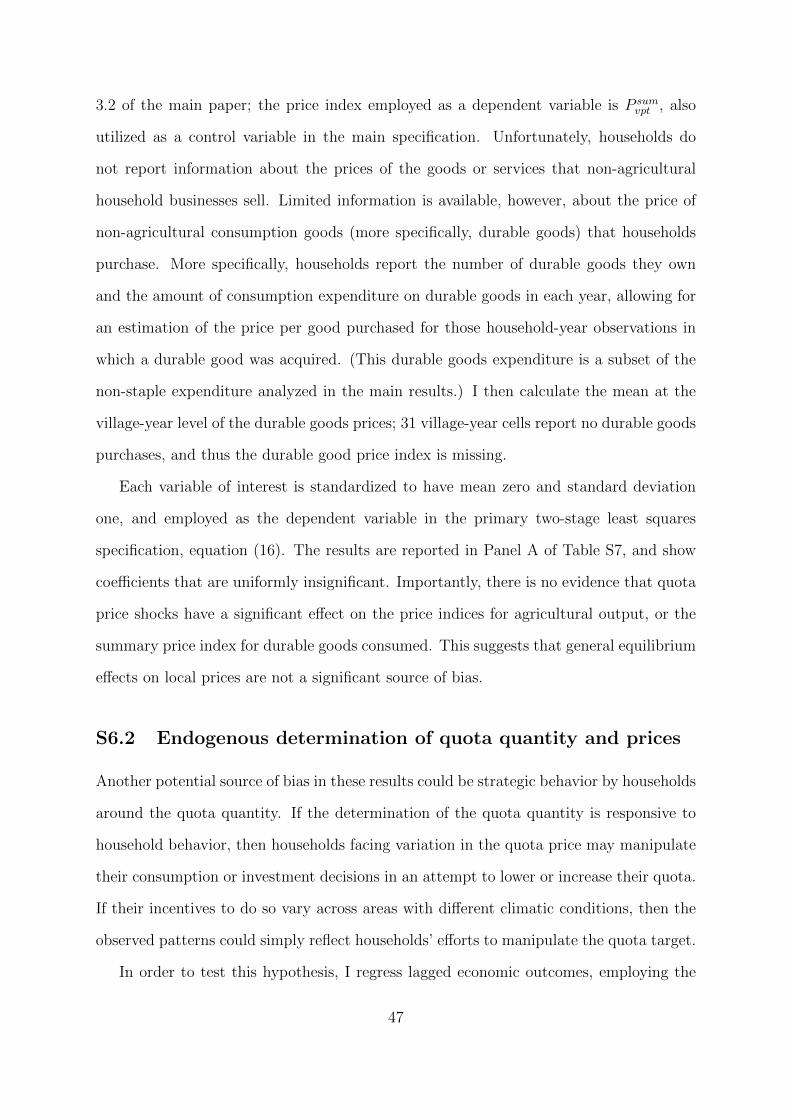
3.2 of the main paper; the price index employed as a dependent variable is P sumvpt , also

utilized as a control variable in the main specification. Unfortunately, households do

not report information about the prices of the goods or services that non-agricultural

household businesses sell. Limited information is available, however, about the price of

non-agricultural consumption goods (more specifically, durable goods) that households

purchase. More specifically, households report the number of durable goods they own

and the amount of consumption expenditure on durable goods in each year, allowing for

an estimation of the price per good purchased for those household-year observations in

which a durable good was acquired. (This durable goods expenditure is a subset of the

non-staple expenditure analyzed in the main results.) I then calculate the mean at the

village-year level of the durable goods prices; 31 village-year cells report no durable goods

purchases, and thus the durable good price index is missing.

Each variable of interest is standardized to have mean zero and standard deviation

one, and employed as the dependent variable in the primary two-stage least squares

specification, equation (16). The results are reported in Panel A of Table S7, and show

coefficients that are uniformly insignificant. Importantly, there is no evidence that quota

price shocks have a significant effect on the price indices for agricultural output, or the

summary price index for durable goods consumed. This suggests that general equilibrium

effects on local prices are not a significant source of bias.

S6.2 Endogenous determination of quota quantity and prices

Another potential source of bias in these results could be strategic behavior by households

around the quota quantity. If the determination of the quota quantity is responsive to

household behavior, then households facing variation in the quota price may manipulate

their consumption or investment decisions in an attempt to lower or increase their quota.

If their incentives to do so vary across areas with different climatic conditions, then the

observed patterns could simply reflect households’ efforts to manipulate the quota target.

In order to test this hypothesis, I regress lagged economic outcomes, employing the

47

same summary measures previously employed, on quota quantity and the interaction of

quantity with the climatic index, including household and province-year fixed effects.

Yivp,t−1 = β1Qivpt + β2Qivpt × Climvp + φivp + νpt + εivpt (17)

The objective is to test whether there is a pattern of reverse causality in which house-

holds’ economic decisions determine the quota quantity they face in a subsequent year,

and whether this relationship varies systematically across areas with different climatic

conditions. The results are shown in Panels B and C of Table S7; the independent vari-

ables are standardized to have mean zero and standard deviation one. The estimated

coefficients are uniformly insignificant.

In addition, it is important to evaluate whether the quota price observed is responsive

to local variation in economic conditions. The measure of quota price that I employ

varies only at the village-year level. Accordingly, I collapse the data to the village-year

level and estimate an equation analogous to equation (18), regressing lagged economic

outcomes on the price and the interaction of the price and the climatic index. This

specification includes 340 village-year cells. The equation of interest can be written as

follows, including village and province-year fixed effects.

Yvp,t−1 = β1P̃qvpt + P̃ q

vpt × Climvp + λvp + νpt + εvpt (18)

The results of estimating equation (18) are reported in Panel D and E of Table S7,

again employing the same summary measures of economic outcomes and standardizing

the explanatory variables to have mean zero and standard deviation one. There is little

evidence of systematic correlations between past economic outcomes and the quota price.

48

S6.3 Attrition

Given that the sample of interest is not a fully balanced panel, there is also the risk of bias

introduced by differential attrition. The core sample includes eight years, and the average

household in the sample is observed in six years. In order to evaluate differences in terms

of households’ duration in the panel, I estimate the following specification in which the

dependent variable is the number of observations for household i, and the independent

variable is the climatic index of interest at the village level. Standard errors are clustered

at the provincial level.

NumObsivp = βClimvp (19)

The results reported in Columns (1) and (2) of Table S8 demonstrate that there is no

systematic difference in the average duration of a household in the panel comparing across

areas with different propensity to cultivate rice.

In addition, I evaluate the hypothesis that the quota price itself predicts exit from the

sample. (This could be a concern if a high quota price generates exit from agriculture,

and non-agricultural households are more likely to exit from the panel.) Using the full

panel, I regress a dummy variable equal to one if the observation corresponds to the final

year in which a particular household is observed on the first, second and third lags of the

quota price, conditional on the same fixed effects employed in the primary specification.

The results reported in Columns (3) and (4) of the same table confirm that there is

no evidence that the first, second or third lags of quota income predict attrition from the

sample. This suggests that attrition is not systematically correlated with the variation

in quota income that is of interest here, and thus is unlikely to be a source of bias.

S6.4 Quota enforcement

In addition, I also evaluate whether quota enforcement differs systematically across areas

with different climatic conditions. Unfortunately, enforcement cannot be measured con-

temporaneously in the primary dataset, as households do not separately report the quota

49

quantity assigned and the quota quantity sold. Evidence from earlier surveys in the same

sample suggests that 95% of quota quantity contracted is delivered. Households that

fail to produce the quota quantity (including households that have exited agriculture)

may face the obligation either to purchase grain at the market price and resell it to the

government, or pay the equivalent in cash.39

In addition, some data is available that can shed some light on variable quota enforce-

ment. First, households report whether any member is a government employee, a village

cadre, or a party member. I can test whether quota income is significantly correlated

with these measures of political influence, and if the correlation varies across villages with

different climatic conditions, estimating the following specification.

Qivpt = β1Xivpt + β2Xivpt × Climvp + +λvp + νpt + Climvp × P sumvpt P

givp,t−2 + ηclimvp × γt

+ +ηclimvp × +ηindvp × γt + εivpt (20)

As reported in Columns (1) through (3) of Table S9, there is some evidence of lower quota

income for government employees, but the relationship does not significantly co-vary with

climatic conditions.40

Second, a separate survey of village leaders reports the total number of party mem-

bers, economic officials, and village officials in the village, a variable I interpret as a rough

measure of enforcement capacity. The survey also reports the quantity of quota grain

delivered relative to the amount contracted in the years 1990 and 1991. I regress these

variables on the climatic index conditional on province-year fixed effects, and find no evi-

dence that enforcement capacity or quota delivery is significantly correlated with climatic

39In this data, village leaders report in surveys in 1990, 1991 and 1993 what fraction of overall quotasales in their village were re-sales of purchase grain or cash payments by households that did not producethe grain themselves; these sales accounted for only 1.5% and 6% of total quota sales, respectively.Households also report in surveys between 1986 and 1991 what fraction of their quota sales correspondedto re-sales and cash payments, and the reported proportions are 1.4% and 1.7% of the total. It shouldbe noted that quota fulfillment in cash may be higher in years in which the quota constitutes a higherproportion of total grain production, in which case these numbers may be underestimates.

40These lower quotas may also reflect the fact that some government employees in rural areas are notallocated land, and thus are not expected to produce grain.

50

conditions. These results, reported in Columns (4) through (8) of Table S9, suggest that

variation in enforcement may be limited.

51

S7 Figures and Tables

Figure S1: Descriptive statistics: Grain quota

(a) Quota income (b) Quota tax

Notes: Figure S1a shows mean household-level quota income by year in hundreds of yuan, as well as the 95th percentileof the distribution of village-level means of quota income by year. Figure S1b shows the mean implicit tax posed by thequota system by year, calculated as the difference between the market and the quota price multiplied by the quotaquantity, as a percentage of total income; again, the 95th percentile of the distribution of village-level means by year isalso included.

Source: Data from the RCRE household panel analyzed by the author.

Table S1: Robustness checks on the first stage

Infra. dummy Quantity res. Quan. rice res. Quota price Quota dummy Quota quan.(1) (2) (3) (4) (5) (6) (7)

Clim. index -.002 -13.653 27.816 -.015 -.0001(.009) (10.960) (55.511) (.019) (.100)

Annual precip. 9.749(14.741)

Annual temp. 114.188(124.304)

Fixed effects Prov.-year Prov.-year Prov.-year Prov.-year Prov.-year VillageClustering Province Province Province Province Province Two-way clusteringObs. 16203 16174 16034 16194 16203 15522 13081F .047 1.416 .229 .608 1.73e-06 .381 .699

Notes: The dependent variable in Column (1) is a dummy variable equal to one if household grain production is equal toquota sales. In Columns (2) and (3) the dependent variables are the residual of quota quantity regressed on village fixedeffects and rice area, respectively; in Column (4), the dependent variable is quota price, and in Column (5) it is a dummyvariable equal to one if a village reports quota phase-out. For Columns (1) through (5), the independent variable is theclimatic index constructed using weather data and annual measures of precipitation and temperature, all normalized tohave mean zero and standard deviation one. In Columns (6) and (7), the dependent variable is quota quantity, and theindependent variables are annualized measurements of precipitation and temperature. Fixed effects and clustering are asreported in the table. Asterisks indicate significance at the ten, five, and one percent level, respectively.

Source: Data from the RCRE household panel analyzed by the author.

52

Table S2: Differential trends and OLS

(1) (2) (3) (4) (5) (6) (7)Agri. input Agri inc. Non-agri. inv. Non-agri. inc. Tot. inc. Outside labor Migration

Panel A: Quota quantity and differential trends

Quota index 1993 .312 .132 .012 .030 .068 .031 .022(.068)∗∗∗ (.029)∗∗∗ (.021) (.014)∗∗ (.021)∗∗∗ (.013)∗∗ (.012)∗

Obs. 15873 15873 15873 15873 15873 15873 15873

Panel B: Ordinary least squares

Quota income .167 .075 .002 .011 .043 .015 .010(lagged) (.026)∗∗∗ (.012)∗∗∗ (.004) (.002)∗∗∗ (.006)∗∗∗ (.003)∗∗∗ (.003)∗∗∗

Obs. 16203 16203 16203 16203 16203 16203 16203

Notes: All specifications include village and province-year fixed effects, the interaction of the climatic index and asummary measure of market prices, climatic index quantile fixed effects interacted with the two year lagged market price,climatic quantile index fixed effects interacted with year fixed effects, and industrial quantile fixed effects interactedwith year fixed effects. Standard errors are estimated employing two-way clustering at the province and year level. Theindependent variable in Panel A is quota quantity in 1993 or the first year in which a village is observed in the panel; theindependent variable in Panel B is quota income, lagged, in hundreds of yuan. Asterisks indicate significance at the ten,five, and one percent level, respectively.

The dependent variable in Column (1) is a summary variable of agricultural investment, calculating using princi-pal component analysis on six variables (area sown, agricultural labor, value of fertilizer employed, value of seedsemployed, investment in animals, and investment in tools). The dependent variable in Column (2) is agricultural income.The dependent variable in Column (3) is a summary variable of non-agricultural investment, calculated using principal com-ponent analysis on four variables (a dummy variable for any new cash investment in non-agricultural machinery, a dummyvariable for any labor invested in a non-agricultural business, and the amount of labor and cash investment reported in non-agricultural businesses). The dependent variable in Column (4) is income from non-agricultural household businesses andwage labor, and the dependent variable in Column (5) is total income. The dependent variable in Column (6) is a dummyvariable for any outside labor; the dependent variable in Column (7) is a dummy variable for any labor worked as a migrant.

Source: Data from the RCRE household panel analyzed by the author.

53

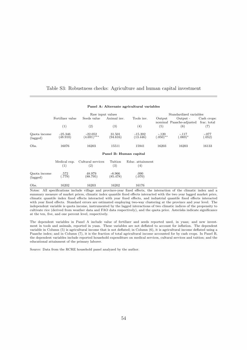
Table S3: Robustness checks: Agriculture and human capital investment

Panel A: Alternate agricultural variables

Raw input values Standardized variablesFertilizer value Seeds value Animal inv. Tools inv. Output Output - Cash crops:

nominal Paasche-adjusted frac. total(1) (2) (3) (4) (5) (6) (7)

Quota income -25.346 -22.052 31.501 -15.202 -.120 -.117 -.077(lagged) (48.910) (4.691)∗∗∗ (94.616) (13.446) (.050)∗∗ (.069)∗ (.052)

Obs. 16076 16203 15511 15941 16203 16203 16133

Panel B: Human capital

Medical exp. Cultural services Tuition Educ. attainment(1) (2) (3) (4)

Quota income .572 48.979 -8.966 .090(lagged) (.779) (88.795) (85.478) (.070)

Obs. 16202 16203 16202 16176

Notes: All specifications include village and province-year fixed effects, the interaction of the climatic index and asummary measure of market prices, climatic index quantile fixed effects interacted with the two year lagged market price,climatic quantile index fixed effects interacted with year fixed effects, and industrial quantile fixed effects interactedwith year fixed effects. Standard errors are estimated employing two-way clustering at the province and year level. Theindependent variable is quota income, instrumented by the lagged interactions of two climatic indices of the propensity tocultivate rice (derived from weather data and FAO data respectively), and the quota price. Asterisks indicate significanceat the ten, five, and one percent level, respectively.

The dependent variables in Panel A include value of fertilizer and seeds reported used, in yuan; and new invest-ment in tools and animals, reported in yuan. These variables are not deflated to account for inflation. The dependentvariable in Column (5) is agricultural income that is not deflated; in Column (6), it is agricultural income deflated using aPaasche index; and in Column (7), it is the fraction of total agricultural income accounted for by cash crops. In Panel B,the dependent variables include reported household expenditure on medical services, cultural services and tuition; and theeducational attainment of the primary laborer.

Source: Data from the RCRE household panel analyzed by the author.

54

Table S4: Alternate specifications

Agri. input Agri inc. Non-agri. inv. Non-agri. inc. Tot. inc. Outside labor Migration(1) (2) (3) (4) (5) (6) (7)

Panel A: Climatic index within 50-kilometer radius

Quota income -.190 -.122 .213 .056 -.053 .050 .173(lagged) (.082)∗∗ (.072)∗ (.115)∗ (.056) (.043) (.054) (.088)∗∗

Obs. 16203 16203 16203 16203 16203 16203 16203

Panel B: Migration and lagged village characteristics

Quota income -.113 -.139 .213 -.0005 -.098 -.048 .046(lagged) (.057)∗∗ (.133) (.144) (.048) (.047)∗∗ (.039) (.039)

Obs. 16145 16145 16145 16145 16145 16145 16145

Panel C: Alternate quota price measures

Quota income -.338 -.181 .216 .078 -.133 .096 .212(lagged) (.136)∗∗ (.064)∗∗∗ (.188) (.047)∗ (.036)∗∗∗ (.042)∗∗ (.086)∗∗

Obs. 16203 16203 16203 16203 16203 16203 16203

Notes: All specifications include village and province-year fixed effects, the interaction of the climatic index and asummary measure of market prices, climatic index quantile fixed effects interacted with the two year lagged market price,climatic quantile index fixed effects interacted with year fixed effects, and industrial quantile fixed effects interactedwith year fixed effects. Standard errors are estimated employing two-way clustering at the province and year level. Theindependent variable is quota income, instrumented by the lagged interactions of two climatic indices of the propensityto cultivate rice (derived from weather data and FAO data respectively), and the quota price. The dependent vari-ables are defined in the notes to Table S2. Asterisks indicate significance at the ten, five, and one percent level, respectively.

In Panel A, the climatic index constructed from precipitation and temperature uses a radius of 50 kilometersaround the county centroid. In Panel B, a range of additional lagged village-level controls (migration levels as a percentageof population, the number of village enterprises, the size of the village labor force, value of productive assets, the quantityof arable land, area sown in grain and cash crops, and total production of grain and cotton) are included. In Panel C, thelinear difference between the quota and market prices is employed as a measure of the quota price shock and interactedwith the climatic indices to construct the instruments.

Source: Data from the RCRE household panel analyzed by the author.

55

Table S5: Alternate specifications, cont.

Agri. input Agri inc. Non-agri. inv. Non-agri. inc. Tot. inc. Outside labor Migration(1) (2) (3) (4) (5) (6) (7)

Panel A: Sample excluding low grain production households

Quota income -.188 -.134 .201 .076 -.064 .050 .177(lagged) (.058)∗∗∗ (.077)∗ (.115)∗ (.059) (.046) (.058) (.090)∗∗

Obs. 16031 16031 16031 16031 16031 16031 16031

Panel B: Sample excluding cases of quota phase-out

Quota income -.260 -.219 .325 .140 -.057 -.004 .187(lagged) (.087)∗∗∗ (.105)∗∗ (.203) (.091) (.071) (.054) (.112)∗

Obs. 14910 14910 14910 14910 14910 14910 14910

Panel C: Sample including additional controls for leading grain market price

Quota income -.174 -.206 .172 .054 -.101 .037 .156(lagged) (.095)∗ (.041)∗∗∗ (.097)∗ (.041) (.034)∗∗∗ (.053) (.077)∗∗

Obs. 16203 16203 16203 16203 16203 16203 16203

Panel D: Sample including fixed effects constructed using FAO index

Quota income -.191 -.027 .204 .052 -.016 .080 .162(lagged) (.079)∗∗ (.099) (.073)∗∗∗ (.051) (.049) (.043)∗ (.068)∗∗

Obs. 16203 16203 16203 16203 16203 16203 16203

Panel E: Sample of heterogeneous cultivation villages

Quota income -.085 .019 .003 -.021 -.00004 .014 .033(lagged) (.102) (.040) (.067) (.036) (.053) (.039) (.021)

Obs. 11576 11576 11576 11576 11576 11576 11576

Notes: All specifications include village and province-year fixed effects, the interaction of the climatic index and asummary measure of market prices, climatic index quantile fixed effects interacted with the two year lagged market price,climatic quantile index fixed effects interacted with year fixed effects, and industrial quantile fixed effects interactedwith year fixed effects. Standard errors are estimated employing two-way clustering at the province and year level. Theindependent variable is quota income, instrumented by the lagged interactions of two climatic indices of the propensityto cultivate rice (derived from weather data and FAO data respectively), and the quota price. The dependent vari-ables are defined in the notes to Table S2. Asterisks indicate significance at the ten, five, and one percent level, respectively.

In Panel A, the sample is restricted to exclude households where quota sales are equal to total reported produc-tion of grain. In Panel B, the sample is restricted to exclude village-years where there is evidence of quota phase-out(no quota sales reported in that year or any subsequent year). In Panel C, interactions between climatic index quantileeffect and leads of the grain market price are included. In Panel D, fixed effects defined using the FAO index are added(quantile-year interactions and quantile-price interactions). In Panel E, the main specification is re-estimated using thesample of heterogeneous cultivation villages.

Source: Data from the RCRE household panel analyzed by the author.

56

Table S6: Additional evidence on channels

Agri. input Agri inc. Non-agri. inv. Non-agri. inc. Tot. inc. Outside labor Migration(1) (2) (3) (4) (5) (6) (7)

Clim. index x price -.004 -.003 .003 .002 -.001 .001 .003(lagged) (.002)∗∗ (.004) (.001)∗∗ (.001)∗ (.002) (.001) (.001)∗∗∗

Education int. .0009 -.001 .0009 -.0002 -.0003 -.0003 .0005(.000) (.001) (.0007) (.0007) (.0006) (.0004) (.0004)

Obs. 16176 16176 16176 16176 16176 16176 16176

Notes: All specifications include village and province-year fixed effects, the interaction of the climatic index and asummary measure of market prices, climatic index quantile fixed effects interacted with the two year lagged marketprice, climatic quantile index fixed effects interacted with year fixed effects, and industrial quantile fixed effectsinteracted with year fixed effects. Standard errors are estimated employing two-way clustering at the province and yearlevel. Standard errors are estimated employing two-way clustering at the province and year level. The dependent vari-ables are defined in the notes to Table S2. Asterisks indicate significance at the ten, five, and one percent level, respectively.

The independent variables include the climatic index-price interaction (employing the weather-derived climatic in-dex), and the triple interaction including a linear variable corresponding to the educational level of the primary laborer inthe household.

Source: Data from the RCRE household panel analyzed by the author.

57

Table S7: Robustness checks

Panel A: Correlated shocks

Ag. price Non ag. price Cadre Party State Taxes Coll. Fees Finesinputs levies

(1) (2) (3) (4) (5) (6) (7) (8) (9)

Quota income -.009 .084 .028 -.034 .062 -.028 .262 .509 -.069(lagged) (.051) (.259) (.046) (.051) (.057) (.212) (.207) (.435) (.312)

Obs. 16203 11978 16176 16195 16203 15832 16065 15992 15979

Panel B: Endogenous determination of quota quantity

Lagged Lagged Lagged Lagged Lagged Lagged LaggedAgri. input Agri inc. Non-agri. inv. Non-agri. inc. Tot. inc. Outside labor Migration

(1) (2) (3) (4) (5) (6) (7)

Quota quantity .112 .053 .086 .004 -.0007 -.010 .007(.153) (.084) (.102) (.031) (.083) (.049) (.038)

Quota quantity int. -.046 -.042 -.084 -.011 .017 .002 -.020(.146) (.066) (.086) (.022) (.067) (.043) (.040)

Obs. 16203 16203 16203 16203 16203 16203 16203

Panel C: Endogenous determination of quota quantity (GAEZ index)

Quota quantity -.075 -.030 .079 .005 -.023 -.039 .004(.069) (.033) (.068) (.029) (.030) (.021)∗ (.013)

Quota quantity int .195 .051 -.124 -.019 .060 .044 -.028(.097)∗∗ (.068) (.093) (.062) (.037) (.032) (.015)∗

Obs. 16203 16203 16203 16203 16203 16203 16203

Panel D: Endogenous determination of quota price

Quota price -.098 -.137 .006 .068 -.039 .053 -.006(.143) (.139) (.087) (.036)∗ (.082) (.054) (.033)

Quota price int. -.010 .102 .043 -.058 .030 -.073 -.010(.101) (.133) (.093) (.032)∗ (.076) (.057) (.037)

Obs. 340 284 340 340 284 340 340

Panel E: Endogenous determination of quota price (GAEZ index)

Quota price -.110 -.036 .052 .019 -.006 -.007 -.010(.066)∗ (.044) (.046) (.014) (.022) (.012) (.016)

Quota price int. .003 -.003 -.010 -.004 -.005 -.007 -.006(.017) (.045) (.031) (.014) (.021) (.021) (.024)

Obs. 340 284 340 340 284 340 340

Notes: In Panel A, the dependent variables are summary measures of prices for agricultural output and non-agricultural(durable) consumption goods, and policy measures measured in the local village and year; the independent variableis lagged quota income, instrumented by the two climatic indices of interest. All specifications include village andprovince-year fixed effects, the interaction of the climatic index and a summary measure of market prices, climatic indexquantile fixed effects interacted with the two year lagged market price, climatic quantile index fixed effects interacted withyear fixed effects, and industrial quantile fixed effects interacted with year fixed effects. Standard errors are estimatedemploying two-way clustering at the province and year level.

In Panels B through E, the dependent variables are lagged values of the primary outcomes of interest in themain analysis, defined in the notes to Table S2. The independent variables in Panels B and C are quota quantity and theinteraction of quota quantity with the climatic index, both standardized to have mean zero and standard deviation one;household and province-year fixed effects are included. The independent variables in Panel D and E are quota price andthe interaction of quota price with the climatic index, both standardized to have mean zero and standard deviation one;data at the village-year level is employed, and village and province-year fixed effects are included. Standard errors areestimated employing two-way clustering at the province and year level. Asterisks indicate significance at the ten, five, andone percent level, respectively.

Source: Data from the RCRE household panel analyzed by the author.

58

Table S8: Attrition

Number observations Final year(1) (2) (3) (4)

Climatic index .420(.390)

FAO index .150(.431)

Quota income lagged .003 -.062(.004) (.075)

Quota income lagged year 2 -.00004(.00003)

Quota income lagged year 3 -9.18e-06(.00006)

Obs. 3798 3798 14772 16203

Notes: In Columns (1) and (2), the dependent variable is the number of years a household is observed in the panel.The independent variables are the two climatic indices of propensity to cultivate rice employed in the main analysis,standardized to have mean zero and standard deviation one; standard errors are clustered at the province level. InColumns (3) and (4), the dependent variable is a dummy variable equal to one if it is the last year in which a householdappears in the panel. The independent variables are quota income lagged and quota income lagged by two and three years;both specifications include village and province-year fixed effects, the interaction of the climatic index and a summarymeasure of market prices, climatic index quantile fixed effects interacted with the two year lagged market price, climaticquantile index fixed effects interacted with year fixed effects, and industrial quantile fixed effects interacted with year fixedeffects. Standard errors are estimated employing two-way clustering at the province and year level. In Column (4), quotaincome is instrumented with the instruments constructed using climatic indices and price. Asterisks indicate significanceat the ten, five, and one percent level, respectively.

Source: Data from the RCRE household panel analyzed by the author.

Table S9: Quota enforcement

Quota quantity Party Economic Cadres Quota fulfilled(1) (2) (3) (4) (5) (6) (7) (8)

Government employee -41.230(11.932)∗∗∗

Employee int. .151(15.377)

Cadre 7.092(10.022)

Cadre int. -8.576(9.687)

Party member -3.031(7.531)

Party member int. -13.778(5.523)∗∗

Climatic index .202 -.117 1.138 -1.752 .003(.158) (.201) (1.831) (1.416) (.015)

Obs. 16128 16147 16155 397 397 396 814 136

Notes: The dependent variable in Columns (1) to (3) is quota quantity; the independent variables are dummy variablesfor a household including a government employee, a party cadre, or a party member, and these variables interacted withthe climatic index for propensity to cultivate rice. The dependent variables in Columns (4) through (8) are the numberof party members, administrative committee members, economic committee members, and cadres reported in the village,and the percentage of the assigned quota reported fulfilled. The quota reported fulfilled is only reported prior to 1993.The specifications in Columns (1) through (3) include village and province-year fixed effects, the interaction of the climaticindex and a summary measure of market prices, climatic index quantile fixed effects interacted with the two year laggedmarket price, climatic quantile index fixed effects interacted with year fixed effects, and industrial quantile fixed effectsinteracted with year fixed effects. Standard errors are estimated employing two-way clustering at the province and yearlevel. The specifications in Columns (4) through (8) include province-year fixed effects, and standard errors clustered atthe village level. Asterisks indicate significance at the ten, five, and one percent level, respectively.

Source: Data from the RCRE household panel analyzed by the author.

59

References

Barrett, Christopher, Mesfin Bezuneh, and Abdillahi Aboud, “Income diversi-

fication, poverty traps and policy shocks in Cote d’Ivoire and Kenya,” Food Policy,

2001, 26, 367–384.

Blattman, Christopher, Nathan Fiala, and Sebastian Martinez, “Generating

skilled self-employment in developing countries: Experimental evidence from Uganda,”

Quarterly Journal of Economics, 2014, 129 (2), 697–752.

Brandt, Loren and Carsten Holz, “Spatial price differences in China: Estimates and

implications,” Economic Development and Cultural Change, 2006, 55 (1), 43–86.

, Jikun Huang, Guo Li, and Scott Rozelle, “Land rights in rural China: Facts,

fictions and issues,” The China Journal, 2002, 47, 67–97.

, Scott Rozelle, and Matthew Turner, “Local government behavior and property

rights formation in rural China,” Journal of Institutional and Theoretical Economics,

2004, 160 (4), 627–662.

Bustos, Paula, Bruno Caprettini, and Jacopo Ponticelli, “Agricultural productiv-

ity and structural transformation: Evidence from Brazil,” American Economic Review,

2016, 106 (6), 1320–65.

Carter, Michael R. and Travis J. Lybbert, “Consumption versus asset smoothing:

testing the implications of poverty trap theory in Burkina Faso,” Journal of Develop-

ment Economics, 2002, 99 (2), 255–264.

, Peter D. Little, Tewodaj Mogues, and Workneh Negatu, “Poverty traps

and natural disasters in Ethiopia and Honduras,” World Development, 2007, 35 (5),

835–856.

60

Foster, Andrew and Mark Rosenzweig, “Agricultural productivity growth, rural

economic diversity, and economic reforms: India, 1970–2000,” Economic Development

and Cultural Change, 2004, 52 (3), 509–542.

Gertler, Paul, Sebastian Martinez, and Marta Rubio-Codina, “Investing cash

transfers to raise long-term living standards,” American Economic Journal: Applied

Economics, 2012, 4 (1), 164–192.

Giesbert, Lena and Kati Schindler, “Assets, shocks, and poverty traps in Rural

Mozambique,” World Development, 2012, 40 (8), 1594–1609.

Gilligan, Daniel, John Hoddinott, and Seyoum Taffesse, “The impact of

Ethiopia’s productive safety net programme and its linkages,” Journal of Development

Studies, 2008, 45 (10), 1684–1706.

Gollin, Douglas, David Lagakos, and Michael Waugh, “The agricultural produc-

tivity gap,” Quarterly Journal of Economics, 2014, 129 (2), 939993.

Hoddinott, John, “Shocks and their consequences across and within households in rural

Zimbabwe,” The Journal of Development Studies, 2006, 42 (2), 301–321.

Huang, Jikuan, Scott Rozelle, and Honglin Wang, “Fostering or stripping rural

China: Modernizing agriculture and rural to urban capital flows,” The Developing

Economies, 2006, 44 (1), 1–26.

Huang, Jikun and Scott Rozelle, “The nature of distortions to agricultural incentives

in China and implications of WTO accession,” 2002.

, , Ruifa Ha, and Ninghui Li, “China’s rice economy and policy: Supply, demand

and trade in the 21st century,” in Mercedita Sombilla, Mahabub Hossain, and Bill

Hardy, eds., Developments in the Asian Rice Economy, Manila: International Rice

Research Institute, 2002.

61

, Yunhua Wu, and Scott Rozelle, “Moving off the farm and intensifying agricul-

tural production in Shandong: A case study of rural labor market linkages in China,”

Agricultural Economics, 2009, 40, 203–18.

Huang, Yipin, Agricultural reform in China: Getting institutions right, Cambridge

University Press, 1998.

IIASA and FAO, 2012. Global Agro-ecological Zones (GAEZ v3.0).

Janzen, Sarah A. and Michael R. Carter, “After the drought: The impact of mi-

croinsurance on consumption smoothing and asset protection,” 2013. NBER Working

Paper No. 19702.

Jedwab, Remi, “Cash crop windfalls and development: On cocoa and cities in Ivory

Coast and Ghana,” 2011.

Jensen, Robert and Nolan Miller, “Giffen behavior and subsistence consumption,”

American Economic Review, Sep. 2008, 98 (1), 1553–1577.

Kaboski, Joseph and Robert Townsend, “A structural evaluation of a large-scale

quasi-experimental microfinance initiative,” Econometrica, 2011, 79 (5), 1357–1406.

Kraay, Aart and David McKenzie, “Do poverty traps exist? Assessing the evidence,”

The Journal of Economic Perspectives, 2014, 28 (3), 127–148.

Kwak, Sungil and Stephen C. Smith, “Regional agricultural endowments and shifts

of poverty trap equilibria: Evidence from Ethiopian panel data,” The Journal of De-

velopment Studies, 2013, 49 (7), 955–975.

Lagakos, David and Michael Waugh, “Selection, agriculture, and cross-country pro-

ductivity differences,” American Economic Review, 2013, 103 (2), 948–80.

Lin, Justin Yifu, “The household responsibility system reform and the adoption of

hybrid rice in China,” Journal of Development Economics, 1991, 36, 353–372.

62

, “Rural reforms and agricultural growth in China,” American Economic Review, 1992,

82 (1), 34–51.

Lu, Feng, “Three grain surpluses: Evolution of China’s grain price and marketing poli-

cies,” 1999.

Naschold, Felix, “The poor stay poor: Household asset poverty traps in rural semi-arid

India,” World Development, 2012, 40 (10), 2033–2043.

, “Welfare dynamics in Pakistan and Ethiopia Does the estimation method matter?,”

The Journal of Development Studies, 2013, 49 (7), 936–954.

Quisumbing, Agnes R. and Bob Baulch, “Assets and poverty traps in rural

Bangladesh,” The Journal of Development Studies, 2013, 49 (7), 898–916.

Rozelle, Scott, Albert Park, Jikun Huang, and Hehui Jin, “Bureaucrat to en-

trepreneur: The changing role of the state in China’s grain economy,” Economic De-

velopment and Cultural Change, 2000, 48 (2), 227–252.

Sadoulet, Elizabeth, Alain de Janvry, and Benjamin Davis, “Cash transfer pro-

grams with income multipliers: PROCAMPO in Mexico,” World Development, 2001,

29 (6), 1043–1046.

Shao, Yun, Xiangtao Fan, Hao Liu, Jianhua Xiao, S. Ross, B. Brisco,

R. Brown, and G. Staples, “Rice monitoring and production estimation using mul-

titemporal RADARSAT,” Remote Sensing of Environment, 2001, 76, 310–25.

Sicular, Terry, “Redefining state, plan and market: China’s reforms in agricultural

commerce,” The China Quarterly, 1995, 144, 1020–1046.

Tang, Shengxiang, Li Ding, and Alain Bonjean, “Rice production and genetic

improvmeent in China,” in Zhonghu He and Alain Bonjean, eds., Cereals in China,

D.F., Mexico: CIMMYT, 2010, pp. 15–34.

63

Wang, Dewen, Jikun Huang, Daniel A. Sumner, and Scott D. Rozelle, “Quo-

tas and grain production in China,” in Scott Rozelle and Daniel A. Sumner, eds.,

Agricultural trade and policy in China, Burlington, VT: Ashgate, 2003, pp. 111–137.

64