The Impact of Oil Price Shocks on the U.S. Stock Market

Lutz Kilian University of Michigan and CEPR

Cheolbeom Park

National University of Singapore

December 31, 2007 Abstract: While there is a strong presumption in the financial press that oil prices drive the stock market, the empirical evidence on the impact of oil price shocks on stock prices has been mixed. This paper shows that the response of aggregate U.S. real stock returns may differ greatly depending on whether the increase in the price of crude oil is driven by demand or supply shocks in the crude oil market. The conventional wisdom that higher oil prices necessarily cause lower stock prices is shown to apply only to oil-market specific demand shocks such as increases in the precautionary demand for crude oil that reflect concerns about future oil supply shortfalls. In contrast, positive shocks to the global demand for industrial commodities cause both higher real oil prices and higher stock prices, which helps explain the resilience of the U.S. stock market to the recent surge in the price of oil. Oil supply shocks have no significant effects on returns. Oil demand and oil supply shocks combined account for 22% of the long-run variation in U.S. real stock returns. The responses of industry-specific U.S. stock returns to demand and supply shocks in the crude oil market are consistent with accounts of the transmission of oil price shocks that emphasize the reduction in domestic final demand. Key Words: Stock returns; oil prices; oil demand shocks, oil supply shocks. JEL Classification: G12, Q43 Acknowledgments: The corresponding author is Lutz Kilian, University of Michigan, Department of Economics, 611 Tappan Street, Ann Arbor, MI 48109-1220, USA. Email: lkilian@umich.edu. We thank the editor and three anonymous referees as well as Ana-María Herrera for very helpful comments on an earlier draft of this paper.

1

1. Introduction

Changes in the price of crude oil are often considered an important factor for understanding

fluctuations in stock prices. For example, the Financial Times on August 21, 2006, attributed the

decline of the U.S. stock market to an increase in crude oil prices caused by concerns about the

political stability in the Middle East (including the Iranian nuclear program, the fragility of the

ceasefire in Lebanon, and terrorist attacks by Islamic militants). The same newspaper on October

12, 2006, argued that the strong rallies in global equity markets were due to a slide in crude oil

prices that same day. Notwithstanding such widely held views in the financial press, there is no

consensus about the relation between the price of oil and stock prices among economists. Kling

(1985), for example, concluded that crude oil price increases are associated with stock market

declines. Chen, Roll and Ross (1986), in contrast, suggested that oil price changes have no effect

on asset pricing. Jones and Kaul (1996) reported a stable negative relationship between oil price

changes and aggregate stock returns. Huang, Masulis, and Stoll (1996), however, found no

negative relationship between stock returns and changes in the price of oil futures, and Wei

(2003) concluded that the decline of U.S. stock prices in 1974 cannot be explained by the

1973/74 oil price increase.

In this paper, we take a fresh look at this question. One limitation of existing work on the

link between oil prices and stock prices is that the price of crude oil is often treated as exogenous

with respect to the economy. It has become widely accepted in recent years that the price of

crude oil since the 1970s has responded to some of the same economic forces that drive stock

prices, making it necessary to control for reverse causality (see Barsky and Kilian 2002, 2004;

Hamilton 2003, 2005; Kilian 2008a,b). This means that cause and effect are not well defined in

regressions of stock returns on oil price changes.

A second limitation of the existing literature is the presumption that it is possible to

2

assess the impact of higher crude oil prices without knowing the underlying causes of the oil

price increase. To the extent that different shocks in the crude oil market have very different

effects on the economy and on the real price of oil, as has been documented in Kilian (2007a,b),

and to the extent that the relative importance of these shocks evolves over time, regressions

relating stock returns to innovations in the price of oil will be biased toward finding no

significant statistical relationships and/or statistical relationships that are unstable over time (see,

e.g., Sadorsky 1999).

In this paper, we address both of these limitations by relating U.S. stock returns to

measures of demand and supply shocks in the global crude oil market, building on a structural

decomposition of fluctuations in the real price of oil. We find that the response of aggregate

stock returns may differ greatly depending on the cause of the oil price shock. The negative

response of stock prices to oil price shocks, often referred to in the financial press, is found only

when the oil price rises due to an oil-market specific demand shock such as an increase in

precautionary demand driven by concerns about future crude oil supply shortfalls. In contrast,

shocks to crude oil production have no significant effect on cumulative stock returns. Finally,

higher oil prices driven by an unanticipated global economic expansion have persistent positive

effects on cumulative stock returns within the first year of the expansionary shock. This result

arises because a positive innovation to the global business cycle will stimulate the U.S. economy

directly, while at the same time driving up the price of oil, thereby indirectly slowing U.S.

economic activity. Since the stimulating effect dominates in the short run, the U.S. stock market

may indeed thrive despite unexpectedly high oil prices. Given that recent increases in the price of

crude oil have been driven primarily by strong global demand for industrial commodities, as

shown below, this fact helps explain why the U.S. stock market so far has proved resilient to

higher oil prices. In contrast, conventional VAR model based on unanticipated oil price changes

3

would have predicted a significant stock market correction in response to the recent oil price

surge.

Our aggregate analysis implies that, on average, in the long run 22% of the variation in

aggregate stock returns during 1975-2006 can be attributed to the shocks that drive the crude oil

market, making oil market fundamentals an important determinant of U.S. stock returns. More

than two thirds of that contribution is driven by shocks to the demand for crude oil. Regardless of

the shock, the impact response of stock returns appears to be driven both by fluctuations in

expected real dividend growth and by fluctuations in expected returns associated with a time-

varying risk premium. We also show that only shocks to the precautionary demand for crude oil

provide an explanation for the negative association between stock returns and inflation found in

previous studies of the postwar period (see, e.g., Kaul and Seyhun 1990).

Of additional interest from an investor’s point of view is the response of industry-specific

stock returns to demand and supply shocks in the crude oil market. We document considerably

stronger and often more significant responses at the industry level to oil demand shocks than to

oil supply shocks, although the degree of sensitivity varied across industries. Our analysis

suggests that the appropriate portfolio adjustments in response to oil price shocks will depend on

the underlying cause of the oil price increase. For example, shares for the gold and silver mining

industry appreciate significantly in response to a positive oil-market specific demand shock,

whereas shares for the petroleum and natural gas stocks remain largely unaffected, and

automobile and the retail sector stocks depreciate persistently and significantly. In contrast, if the

same increase in oil prices is driven by innovations to global real economic activity, the share

prices of all four industries will increase within the first year, albeit to a different degree.

The responses of industry-level stock returns also shed light on the transmission of oil

demand and oil supply shocks to the U.S. stock market. We find evidence that the transmission is

4

driven not by domestic cost or productivity shocks, but by shifts in the final demand for goods

and services. Our results suggest that the total cost share of energy is not an important factor in

explaining differences in the responses of real stock returns across manufacturing industries,

which casts doubt on the interpretation of oil price shocks as aggregate productivity shocks.

Moreover, outside of the energy sector, some of the strongest responses to oil demand shocks are

found in the automotive industry, in the retail industry, in consumer goods, and in tourism-

related sectors such as restaurants and lodging, consistent with the view that oil price shocks are

primarily shocks to the demand for goods and services rather than supply shocks for the U.S.

economy (also see, e.g., Hamilton 1988; Dhawan and Jeske 2006; Edelstein and Kilian 2007a,b).

We also relate our analysis to studies emphasizing the endogenous monetary policy

response to oil price shocks (see, e.g., Bernanke, Gertler and Watson 1997). In particular, we

investigate the question of whether monetary policy responds to oil demand and supply shocks.

We show that the responses to oil demand shocks are statistically significant at the 10% level,

but the overall cumulative impact on changes in the Federal Funds rate is negligible. Finally, we

highlight implications of our analysis for dynamic stochastic general equilibrium (DSGE)

models of the link between oil prices and stock prices. The remainder of the paper is organized

as follows. Section 2 describes the empirical methodology. Section 3 contains the empirical

results. Section 4 focuses on industry-level stock returns and the nature of the transmission of

shocks in the crude oil market to the U.S. stock market. Section 5 contains concluding remarks.

2. Dynamics of Aggregate Stock Return Responses to Structural Oil Shocks

2.1. Data Description

Our data include a measure of the percent change in world crude oil production, the real price of

crude oil imported by the U.S., an indicator of the global business cycle in industrial commodity

markets, and selected U.S. stock market variables. All data used in this paper are monthly. The

5

sample period is 1973.1-2006.12. The starting date is dictated by the availability of the crude oil

production data.

We construct the percent change in global production of crude oil based on production

data from the U.S. Department of Energy. Our measure of the real price of oil is based on U.S.

refiner’s acquisition cost of crude oil, as reported by the U.S. Department of Energy for the

period starting in 1974.1, and has been extrapolated back to 1973.1 following Barsky and Kilian

(2002). The nominal price of oil was deflated by the U.S. consumer price index (CPI) available

from the BLS. Finally, we rely on a measure of monthly global real economic activity designed

to capture across-the board shifts in the global demand for industrial commodities.1 That measure

is constructed from an equal-weighted index of the percent growth rates obtained from a panel of

single voyage bulk dry cargo ocean shipping freight rates measured in dollars per metric ton. The

rationale of using this index is that increases in dry cargo ocean shipping rates, given a largely

inelastic supply of suitable ships, will be indicative of higher demand for shipping services

arising from increases in global real activity (see Kilian (2007a) for further discussion).

The underlying panel data set of shipping rates is based on Drewry’s Shipping Monthly,

Ltd. It includes shipping rates for dry cargoes such as iron ore, coal, grains, fertilizer, and scrap

metal for all major shipping routes in the world. The construction of the index controls for fixed

effects associated with shipping routes, ship sizes and types of cargo. The nominal index is

deflated using the U.S. CPI and subsequently linearly detrended to remove a secular trend in the

cost of shipping, resulting in a stationary index of fluctuations in global real activity.

One of the chief advantages of this monthly index based on bulk dry cargo ocean freight

rates is that it automatically incorporates the effects of increased real activity in newly emerging

1 The term real economic activity in this paper is understood to refer to real economic activity that affects industrial commodity markets rather than the usual broader concept of real economic activity underlying world real GDP. This distinction is necessary because an increase in value added in the service sector, for example, is likely to have a very different effect on global demand for industrial commodities than an increase in value added in manufacturing.

6

economies such as China or India, for which monthly industrial production data are not available.

In contrast, more conventional measures of monthly global real activity such as the OECD

industrial production index exclude real activity in China and India. Since much of the recent

surge in demand for industrial commodities (including crude oil) is thought to be driven by

increased demand from India and China, the use of a truly global measure of real activity and

one specifically geared toward industrial commodity markets is essential, although for other time

periods the choice of the index typically makes little difference, as discussed in Kilian (2007a).

The aggregate U.S. real stock return is constructed by subtracting the CPI inflation rate

from the log returns of the Center for Research in Security Prices (CRSP) value-weighted market

portfolio.2 The aggregate U.S. dividend-growth rate is constructed from monthly returns on the

CRSP value-weighted market portfolio with and without dividends following Torous, Valkanov,

and Yan (2005).

2.2. Empirical Methodology

Existing studies of the relationship between oil prices and real stock returns suffer from two

limitations. First, many previous empirical and theoretical models of the link between oil prices

and stock prices have been constructed under the premise that one can think of varying the price

of crude oil, while holding all other variables in the model constant (see, e.g., Wei 2003). In

other words, oil prices are treated as strictly exogenous with respect to the global economy. This

premise is not credible (see, e.g., Barsky and Kilian 2002, 2004; Hamilton 2003). There are good

theoretical reasons and there is strong empirical evidence that global macroeconomic

fluctuations have influenced the price of crude oil since the 1970s (see Kilian 2007a, 2008a). For

example, it is widely accepted that a global business cycle expansion (as in recent years) tends to

2 The CRSP data were obtained from http://wrds.wharton.upenn.edu.

7

raise the price of crude oil.3 The fact that the same economic shocks that drive macroeconomic

aggregates (and thus stock returns) may also drive the price of crude oil makes it difficult to

separate cause and effect in studying the relationship between oil prices and stock returns.

Second, even if we were to control for reverse causality, existing models postulate that

the effect of an exogenous increase in the price of oil is the same, regardless of which underlying

shock in the oil market is responsible for driving up the price of crude oil. Recent work by Kilian

(2007a) has shown that the effects of demand and supply shocks in the crude oil market on U.S.

macroeconomic aggregates are qualitatively and quantitatively different, depending on whether

the oil price increase is driven by oil production shortfalls, by a booming world economy, or by

shifts in precautionary demand for crude oil that reflect increased concerns about future oil

supply shortfalls. It is quite natural to expect similar differences in the effect of these shocks on

stock returns. Since major oil price shocks historically have been driven by varying combinations

of these demand and supply shocks, their effect on stock returns is bound to be different from

one episode to the next. In fact, to the extent that exogenous demand shocks in the crude oil

market have direct effects on the U.S. economy in addition to their indirect effects through the

real price of oil, it is not possible to think of an innovation to the real price of oil while holding

everything else constant.

In this paper, we address both of these limitations with the help of a structural VAR

model that relates U.S. stock market variables to measures of demand and supply shocks in the

global crude oil market. This model builds on a structural VAR decomposition of the real price

of crude oil proposed in Kilian (2007a). A similar approach has also been used in Kilian (2007b)

to study the evolution of U.S. gasoline prices. Specifically, we estimate a structural VAR model

based on monthly data for the vector time series tz , consisting of the percent change in global 3 As noted by Hamilton (2005), “it is clear … that demand increases rather than supply reductions have been the primary factor driving oil prices over the last several years.”

8

crude oil production, the measure of real activity in global industrial commodity markets

discussed above, the real price of crude oil, and the U.S. stock market variable of interest (say,

real stock returns) in the order given.

Given the possibility that some responses may be delayed by more than a year, the VAR

model allows for two years’ worth of lags. The structural representation of this VAR model is

(1) 24

01

t i t i ti

A z A zα ε−=

= + +∑ ,

where tε denotes the vector of serially and mutually uncorrelated structural innovations. Let te

denote the reduced form VAR innovations such that 10t te A ε−= . The structural innovations are

derived from the reduced form innovations by imposing exclusion restrictions on 10A− . Our

model imposes a block-recursive structure on the contemporaneous relationship between the

reduced-form disturbances and the underlying structural disturbances. The first block constitutes

a model of the global crude oil market. The second block consists of U.S. real stock returns.

2.2.1. Structural Shocks

In the oil market block, we attribute fluctuations in the real price of oil to three structural shocks:

1tε denotes shocks to the global supply of crude oil (henceforth “oil supply shock”); 2tε captures

shocks to the global demand for all industrial commodities (including crude oil) that are driven

by global real economic activity (“aggregate demand shock”); and 3tε denotes an oil-market

specific demand shock. The latter shock is designed to capture shifts in precautionary demand

for crude oil that reflect increased concerns about the availability of future oil supplies that are

by construction orthogonal to the other shocks (“oil-specific demand shock”).

Below we will use the terms oil-market specific demand shock and precautionary

demand shock interchangeably. Precautionary demand arises from the uncertainty about

9

shortfalls of expected supply relative to expected demand. It reflects the convenience yield from

having access to inventory holdings of oil that can serve as insurance against an interruption of

oil supplies (see Alquist and Kilian (2007) for a formal analysis). Such an interruption could

arise because of unexpected growth of demand, because of unexpected declines of supply or

because of both. One can interpret precautionary demand shocks as arising from a shift in the

conditional variance, as opposed to the conditional mean, of oil supply shortfalls. Such shifts in

uncertainty may arise even controlling for the global business cycle and the global supply of

crude oil.

Although fluctuations in 3tε potentially could reflect other oil-market specific demand

shocks, as discussed in Kilian (2007a) there are strong reasons to believe that this shock

effectively represents exogenous shifts in precautionary demand. First, there are no other

plausible candidates for exogenous oil-market specific demand shocks. Second, the large impact

effect of oil-market specific shocks documented in section 3.1 is difficult to reconcile with

shocks not driven by expectation shifts. Third, as documented below, the timing of these shocks

and the direction of their effects are consistent with the timing of exogenous events such as the

outbreak of the Persian Gulf War that would be expected to affect uncertainty about future oil

supply shortfalls on a priori grounds. Fourth, the overshooting of the price of oil in response to

oil-market specific demand shocks documented in section 3.1 coincides with the predictions of

theoretical models of precautionary demand shocks driven by increased uncertainty about future

oil supply shortfalls (see Alquist and Kilian 2007). Finally, the movements in the real price of oil

induced by this shock are highly correlated with independent measures of the precautionary

demand component of the real price of oil based on crude oil futures prices. Using oil futures

market data since 1989, Alquist and Kilian (2007) show that this correlation may be as high as

80% notwithstanding the use of a completely different data set and methodology.

10

In the U.S. stock market block, there is only one structural innovation. Whereas 1 2, ,t tε ε

and 3tε may be viewed as fully structural, 4tε is not a truly structural shock. We refer to the latter

shock as an innovation to real stock returns not driven by global crude oil demand or crude oil

supply shocks. We do not attempt to disentangle further the structural shocks driving stock

returns, since in this paper we are solely concerned with the impact of structural shocks in the

crude oil market on the U.S. stock market.

2.2.2. Identifying Assumptions

The model imposes the following identifying assumptions resulting in a recursively identified

structural model of the form:

(2)

supply111 1

21 222 2

31 32 333 3. .

41 42 43 444

0 0 00 0

0

global oil production oil shockt t

global real activity aggregate demand shockt t

t real price of oil oil specific dt t

U S stock returnst

aea ae

ea a aea a a ae

εεε

Δ

−

⎛ ⎞ ⎡ ⎤⎜ ⎟ ⎢ ⎥⎜ ⎟ ⎢ ⎥≡ =⎜ ⎟ ⎢ ⎥⎜ ⎟ ⎢ ⎥

⎣ ⎦⎝ ⎠ 4

emand shock

other shocks to stock returnstε

⎛ ⎞⎜ ⎟⎜ ⎟⎜ ⎟⎜ ⎟⎝ ⎠

The nature and origin of the identifying assumptions is discussed in more detail below.

Global Oil Market Block

The three exclusion restrictions in the first block of (2) are consistent with a vertical short-run

global supply curve of crude oil and a downward sloping demand curve. Shifts of the demand

curve driven by either of the two oil demand shocks result in an instantaneous change in the real

price of oil, as do unanticipated oil supply shocks that shift the vertical supply curve. Following

Kilian (2007a), these identifying restrictions may be motivated as follows: (1) crude oil supply

will not respond to oil demand shocks within the month, given the costs of adjusting oil

production and the uncertainty about the state of the crude oil market; (2) increases in the real

price of oil driven by shocks that are specific to the oil market will not lower global real

11

economic activity within the month; and (3) innovations to the real price of oil that cannot be

explained by oil supply shocks or shocks to the aggregate demand for industrial commodities

must be demand shocks that are specific to the oil market.

U.S. Stock Market Block

The second block consists of only one equation. The block-recursive structure of the model

implies that global crude oil production, global real activity and the real price of oil are treated as

predetermined with respect to U.S. real stock returns. Whereas U.S. real stock returns are

allowed to respond to all three oil demand and oil supply shocks on impact, the maintained

assumption is that 4tε does not affect global crude oil production, global real activity and the real

price of oil within a given month, but only with a delay of at least one month. This assumption is

implied by the standard approach of treating innovations to the price of oil as predetermined with

respect to the U.S. economy (see, e.g., Lee and Ni 2002). It implies the three exclusion

restrictions in the last column of 10 .A−

3. Structural VAR Estimates

3.1. The Effects of Crude Oil Demand and Supply Shocks on the Real Price of Oil

It is useful to review the responses of the real price of crude oil to the three structural shocks

, 1,2,3,jt jε = as reported in Figure 1, before turning to the effect of the same shocks on U.S. real

stock returns. The oil supply shock has been normalized to represent a negative one standard

deviation shock, while the aggregate demand shock and oil-market specific demand shock have

been normalized to represent positive shocks such that all three shocks would tend to raise the

real price of oil. One-standard error and two-standard error bands are indicated by dashed and

dotted lines. All intervals have been computed based on appropriate bootstrap methods. The

central result in Figure 1 is that these three shocks have very different effects on the real price of

12

oil. For example, an unexpected increase in precautionary demand for oil causes an immediate

and persistent increase in the real price of oil, followed by a gradual decline; an unexpected

increase in global demand for all industrial commodities causes a delayed, but sustained increase

in the real price of oil; whereas an unanticipated oil production disruption causes a transitory

increase in the real price of oil within the first year.

While impulse responses help us assess the timing and magnitude of the responses to

one-time demand or supply shocks in the crude oil market, historical episodes of oil price shocks

are not limited to a one-time shock. Rather they involve a vector sequence of shocks, often with

different signs at different points in time. If we want to understand the cumulative effect of such

a sequence of shocks, it becomes necessary to construct a historical decomposition of the effect

of each of these shocks on the real price of oil.4 The historical decomposition of fluctuations in

the real price of oil in Figure 2 suggests that oil price shocks historically have been driven

mainly by a combination of aggregate demand shocks and precautionary demand shocks, rather

than oil supply shocks. For example, the increase in the real price of oil after 1978 was primarily

driven by the superimposition of strong global demand and a sharp increase in precautionary

demand in 1979 with only minor contributions from oil supply shocks. Likewise the build-up in

the real price of oil after 2003 was driven almost entirely by the cumulative effects of positive

global demand shocks.5 We will return to this point below.

3.2. Responses and Variance Decomposition of U.S. Real Stock Returns

The upper panel of Figure 3 shows the cumulative impulse responses of the CRSP value-

weighted stock returns to each of the three demand and supply shocks in the crude oil market.

4 This may be accomplished by simulating the path of the real price of oil from model (1) under the counterfactual assumption that a given shock is zero throughout the sample period. The difference between this counterfactual path and the actual path of the real price of oil measures the cumulative effect of the shock at each point in time. 5 These results are broadly consistent with other evidence and theoretical accounts of the history of the crude oil market. For further discussion see Barsky and Kilian (2002, 2004) and Kilian (2007a, 2008a).

13

Figure 3 underscores the point that the responses of aggregate real stock returns may differ

substantially, depending on the underlying cause of the oil price increase. Figure 3 shows that

unanticipated disruptions of crude oil production do not have a significant effect on cumulative

U.S. stock returns at the 10% level. In contrast, an unexpected increase in the global demand for

industrial commodities driven by increased global real economic activity will cause a sustained

increase in U.S. stock returns that persists for 11 months and is partially statistically significant

at the 10% level for the first 7 months. Finally, an increase in the precautionary demand for oil

all else equal would cause persistently negative U.S. stock returns that are significant at the 10%

level for the first 6 months, as shown in the right panel.

The variance decomposition in Table 1 quantifies how important 1 2, ,t tε ε and 3tε have

been on average for U.S. stock returns. In the short-run, the effect of these three shocks is

negligible. On impact, only about 1% of the variation in U.S. real stock returns is associated with

shocks that drive the global crude oil market. The explanatory power quickly increases, as the

horizon is lengthened. In the long run, 22% of the variability in U.S. real stock returns is

accounted for by the three structural shocks that drive the global crude oil market, suggesting

that shocks in global oil markets are an important fundamental for the U.S. stock market. With

11% by far the largest contributor to the variability of returns are oil-market specific demand

shocks. This estimate reflects the importance of expectations-driven shifts in precautionary

demand for crude oil. Aggregate demand shocks account for about 5%. Oil supply shocks only

account for about 6% of the variability of returns. Overall, oil demand shocks in the crude oil

market account for 16%, whereas oil supply shocks only account for 6% of the long-run

variation in U.S. aggregate real stock returns.

3.3. Responses and Variance Decompositions of U.S. Real Dividend Growth

We also investigated the response of real dividend growth rates to demand and supply shocks in

14

the crude oil market. Rather than modeling the contemporaneous relationship between U.S. real

stock returns and U.S. real dividend growth, which is neither feasible nor necessary for our

purposes, we re-estimate model (1) with real dividend growth replacing real stock returns as the

last element of .tz The cumulative responses of the dividend-growth rate to each shock are

shown in the lower panel of Figure 3. Consistent with recent work by Lettau and Ludvigson

(2005) we find that expected dividend growth does not remain constant in response to oil

demand and oil supply shocks. Moreover, there is strong evidence that different shocks have

different effects on real dividends. Unanticipated oil supply disruptions lower real dividends. The

response is significantly negative at the 10% level after 5 months. Positive aggregate demand

shocks increase real dividends persistently. The response is significant at the 10% level at most

horizons. Finally, positive shocks to precautionary demand persistently lower real dividends. The

response is significant at the 10% level at all horizons. The variance decomposition in Table 2

shows that, in the long run, 23% of the variation in real dividend growth can be accounted for by

shocks that drive the crude oil market, more than two thirds of which is associated with oil

demand shocks. In contrast, the combined explanatory power of these shocks on impact is only

2%. These results are broadly similar to the earlier findings for real stock returns.

3.4. Broader Implications of the Impulse Response Analysis

The preceding analysis has several implications for the analysis of the effect of oil price shocks

on the U.S. stock market. First, it highlights serious limitations in conventional accounts of the

link between oil prices and stock returns. Second, our analysis explains why the dramatic surge

in oil prices in recent years has not caused a stock market decline so far. Third, it implies that

VAR models that relate U.S. stock returns to unanticipated changes in the price of oil are

valuable in characterizing average tendencies in the data, but can be very misleading when

discussing the effects of specific oil price shocks. Fourth, our analysis helps explain why

15

regressions of U.S. stock returns on the price of oil tend to be unstable. Fifth, our analysis

illustrates the point that the price of oil must not be treated as exogenous in the construction of

DSGE models of the link between oil prices and stock prices.

3.4.1. Why the Origin of Oil Price Shocks Matters

A striking result in Figure 3 is the fact that, even after 12 months, oil supply disruptions have no

significant effect on cumulative stock returns. The lack of a significant response of cumulative

returns is consistent with the weak response of the real price of oil shown in Figure 1; yet it

raises the question of what – if not adverse oil supply shocks – accounts for the anecdotal

evidence of large declines in stock prices associated with major political disturbances in the

Middle East. The answer lies in sharp increases in precautionary demand. As shifts in

precautionary demand are ultimately driven by expectations about the shortfalls of future oil

supplies and such expectations can change almost instantaneously in response to political events

in the Middle East, such shocks may trigger an immediate and sharp increase in precautionary

demand that is reflected in an immediate jump in the real price of oil (see Figure 1) as well as an

immediate drop in stock prices (see Figure 3).

The latter situation is consistent with the August 21, 2006, Financial Times quote used in

the introduction. However, this does not mean that higher oil prices will always be bad news for

the stock market. Specifically, an unexpected global aggregate demand expansion will cause

both cumulative real stock returns and the real price of crude oil to rise. This may be seen by

comparing the second panel of Figure 3 with the response of the real price of oil to the same

shock in Figure 1. Hence, the October 12 quote in the Financial Times, linking falling oil prices

to rising stock prices, is not obviously true. In fact, without knowing why oil prices fell that day,

we cannot attribute the rise in stock prices to the price of oil. If there had been a sudden influx of

good news about the Middle East that day, the Financial Times might have been on target. If the

16

observed fall in crude oil prices instead had reflected an unexpected slowdown of the global

economy (which seems not entirely unlikely given the slowdown of the U.S. economy around

this time), all else equal, Figure 3 would have predicted a decline in stock prices. In that case, the

true reason for the rise in stock prices that day would have been something else entirely. Thus,

there are no simple and stable rules linking oil prices and stock prices. The nature of this

relationship depends on which of the three shocks are driving the price of oil.

It may seem puzzling at first that an aggregate demand shock that after all tends to raise

the real price of oil (as shown in Figure 1) would be capable of generating a temporary

appreciation of U.S. stocks (as shown in Figure 3). This finding illustrates the dangers of

incorrectly invoking the ceteris paribus assumption in linking changes in the real price of oil to

stock market outcomes. As discussed in Kilian (2007a), an unanticipated increase in global

demand for industrial commodities has two effects on U.S. stock returns. One effect is a direct

stimulus for the U.S. economy and hence the U.S. stock market. The other effect is indirect. As

the global aggregate demand expansion raises the real price of oil, it slows U.S. economic

activity and depresses the U.S. stock market. The response estimate shown in Figure 3 shows

that the stimulating effect tends to dominate in the first year following this shock, whereas the

depressing effect reaches its full strength only with a delay.

3.4.2. Why the Stock Market Has Proved Resilient to Higher Oil Prices in Recent Years

Our approach provides a direct answer to the question of why the stock market in recent years

has proved surprisingly resilient to higher oil prices. As Figure 2 shows the increase in oil prices

in 2004-2006 was driven almost exclusively by unanticipated strong global demand for industrial

commodities, driven in important part by strong economic growth in Asia. Given the response

estimates for global aggregate demand shocks in Figure 3 we know that a series of positive

aggregate demand shocks could sustain the U.S. stock market for several years. The absence of a

17

stock market correction only seems puzzling when ignoring the direct stimulating effect of

positive aggregate demand shocks in global industrial commodity markets. As long as that

stimulus persists and there are no major precautionary demand shocks or adverse supply shocks,

oil price increases do not necessarily constitute a reason for stock prices to fall.

3.4.3. The Limitations of VAR Models of the Responses to Unanticipated Oil Price Changes

The standard approach in the literature is to estimate the responses of macroeconomic aggregates

to an unanticipated innovation in the price of crude oil (see, e.g., Lee and Ni (2002) for an

application to U.S. industrial production). In its simplest form this approach involves a

recursively identified VAR model for [ , . . ]t t tz real price of oil U S stock returns≡ of the form

(3) 24

01

t i t i ti

A z A zα ε−=

= + +∑ ,

where

(4) 111 1. .

21 222 2

0real price of oil real oil price shockt t

t U S stock returns other shocks to stock returnst t

aee

a aeεε

⎛ ⎞ ⎛ ⎞⎡ ⎤≡ =⎜ ⎟ ⎜ ⎟⎢ ⎥

⎣ ⎦⎝ ⎠ ⎝ ⎠.

The exclusion restriction reflects the fact that innovations to the price of oil are treated as

predetermined with respect to stock returns (and other domestic macroeconomic variables). This

assumption is standard in the literature. For our purposes, it is immaterial whether this model is

augmented to include additional variables, as long as the real price of oil is ordered first. While

this approach is valuable in characterizing average tendencies in the data (and indeed is logically

consistent with our approach given that innovations to the real price of oil can be expressed as a

weighted average of predetermined oil demand and oil supply shocks), it can be very misleading

when discussing the effects of specific oil price shock episodes.

A case in point is the surge in oil prices in 2004-2006. In fact, a researcher following the

18

conventional approach and relying on model (3) would have concluded that the stock price

should unambiguously fall in response to an unanticipated increase in the price of oil. Figure 4 is

based on a bivariate VAR model with the real price of oil ordered first. It shows the conventional

result that an unanticipated increase in the real price of oil causes cumulative stock returns to

fall.6 The decline is statistically significant one month after the shock. As we know, this decline

is not what happened following the oil price shocks in 2004-2006 because these specific shocks

had a composition that greatly differed from the average shock over the sample period. This

example illustrates that it is important to understand why oil prices have increased when

assessing the likely consequences of that increase. The same unanticipated increase in oil prices

can be consistent with a sharp decline or a temporary increase in stock prices, depending on the

composition of the underlying oil demand and oil supply shocks. Our methodology allows that

distinction, whereas the conventional approach used by Lee and Ni (2002) and others does not.

3.4.4. The Instability of Reduced-Form Regressions of Stock Returns on Oil Price Changes

The results in Figure 3 suggest caution in interpreting empirical results based on reduced form

regressions of real stock returns on oil price changes. Figure 2 shows that the relative importance

of any one shock in the crude oil market for the real price of oil tends to vary over time. Clearly,

if over a given sample period one of the three shocks is more prevalent, it will dominate the

average responses to the oil price increase estimated for that period. Whether or not one finds a

stable negative relationship in the data then really becomes a question of how important

aggregate demand shocks are for that period relative to precautionary demand shocks. This fact

helps explain in part why existing empirical evidence using reduced-form regressions has been

mixed, as noted in the introduction.

6 The qualitative results reported for the bivariate VAR model are not sensitive to the lag order.

19

3.4.5. Implications for DSGE Models of the Link from Oil Prices to Stock Prices

Our analysis also has important implications for the construction of DSGE models of the effect

of oil price shocks on stock markets. The standard approach in the DSGE literature, exemplified

by Wei (2003), is to postulate that oil prices follow an exogenous ARMA(1,1) process. That

assumption not only rules out feedback from the U.S. economy to the oil market, which seems

implausible in light of recent research, but it also specifically rules out direct effects from

unanticipated aggregate demand shocks on the U.S. economy. This fact makes it difficult to

interpret the theoretical results in Wei (2003). 7

Quite apart from these methodological differences, our analysis provides a potential

explanation for the difficulties Wei encountered in linking the stock market decline of 1974 to

the oil price increase of 1973/74. Since unanticipated aggregate demand shocks played a major

role in driving up the price of oil in 1973/74, as documented in Barsky and Kilian (2002) and in

Kilian (2008a), the empirical finding in Wei (2003) that higher oil prices apparently seem to

have had little impact on the stock market following the oil price shock of 1973/74 is not

surprising. This is what one would expect if positive aggregate demand shocks in global

industrial commodity markets offset the effects of negative oil supply shocks and positive

precautionary demand shocks. Thus, we tend to agree with the substance of Wei’s findings. In

fact, Barsky and Kilian (2002) made the case that the recession of 1974/75 (and the associated

decline in the stock prices) had little to do with the 1973/74 oil price shock and was driven

primarily by domestic economic policies. On the other hand, our analysis suggests that, contrary

to Wei’s finding, oil price shocks may indeed be associated with a sharp decline in stock market

values, provided the oil price shock is driven primarily by positive precautionary demand shocks.

7 Recent DSGE models by Bodenstein, Erceg and Guerrieri (2007) and Nakov and Pescatori (2007), building on the analysis in Kilian (2007a,b), have successfully endogenized the price of oil, but to date no such DSGE model exists for the U.S. stock market.

20

3.5. What Is Driving The Response of U.S. Real Stock Returns?

The cumulative return responses shown in the upper panel of Figure 3 imply that not all of the

adjustment of real stock returns in response to oil demand and oil supply shocks occurs on

impact. This finding, although at odds with early models of market efficiency based on the

counterfactual premise of constant expected returns, is fully consistent with modern models of

time-varying expected returns (see, e.g., Campbell, Lo and MacKinlay 1997, Cochrane 2005).

Building on the analysis in Campbell (1991), by construction, the impact response of stock

returns to a given oil demand or oil supply shock must reflect either variation in expected real

dividend growth or variation in expected returns (reflecting the evolution of the risk premium)

suitably discounted to the date of the shock. This fact allows us to construct a formal statistical

test of whether the impact response of stock returns is fully accounted for by either expected

returns or expected dividend growth. Following Campbell (1991), unexpected changes in log real

stock returns can be approximated by:

(5) 1 10 0

( ) i it t t t t i t t i

i i

r E r E d E dρ ρ∞ ∞

− + − += =

⎛ ⎞ ⎛ ⎞− = Δ − Δ⎜ ⎟ ⎜ ⎟⎝ ⎠ ⎝ ⎠∑ ∑ 1

1 1

i it t i t t i

i i

E r E rρ ρ∞ ∞

+ − += =

⎡ ⎤⎛ ⎞ ⎛ ⎞− −⎢ ⎥⎜ ⎟ ⎜ ⎟⎝ ⎠ ⎝ ⎠⎣ ⎦∑ ∑ ,

where tdΔ is the dividend-growth rate at time t, ρ ≡ + −1 1/ (log( exp( ))d p , and pd − is the

average log dividend-price ratio. Equation (5) states that unanticipated changes in real stock

return from period 1t − to period t must be due to revised expectations about future dividend

growth and/or revised expectations about future returns. Using reduced-form VAR methods,

Campbell (1991) concluded that real stock returns were more closely related to fluctuations in

expected returns than to fluctuations in expected dividend growth. In this paper, we focus on the

related, but different and more specific question of whether the responses of stock returns to

specific demand and supply shocks in the crude oil market are driven by fluctuations in expected

returns or by fluctuations in expected dividend growth.

21

This requires a reinterpretation of equation (5) in terms of the responses to unanticipated

disturbances in the crude oil market. Without loss of generality, suppose that we normalize all

expectations as of period 1t − in equation (5) to zero. Let iψ and iδ denote the responses of real

stock returns and real dividend growth, respectively, at horizon i to a given structural shock in

the crude oil market. These responses may be obtained from the two VAR models described

earlier. The response coefficients represent departures from the baseline induced by a given

shock. Hence, changes in expected returns and changes in expected dividend growth relative to

the baseline in response to an unexpected disturbance in the crude oil market can be written as:

0011 0)()()( ψψ =−=−=− −− ttttttt rErErEr ,

1( ) ( ) 0i i i it t i t t i i iE d E dρ ρ ρ δ ρ δ+ − +Δ − Δ = − = ,

1( ) ( ) 0i i i it t i t t i i iE r E rρ ρ ρψ ρψ+ − +− = − = .

Recall that 0ψ denotes the response of tr to a shock in the oil market in month ,t as measured by

the first element of the impulse response function of real stock returns. Similarly, the revisions of

the expected values of future real dividend growth and real stock returns are given by the

additional elements of the impulse response functions already estimated in sections 3.2 and 3.3.

This allows us to test formally whether the impact change in real stock returns arising from a

given demand or supply shock in the global crude oil market can be attributed in its entirety to

revisions of expected real dividend growth. This null hypothesis can be stated as:

0 :H 36

00 0

i ij ij ij

i i

ψ ρ δ ρ δ∞

= =

= ≈∑ ∑ ,

where ijδ denotes the response of real dividend growth to shock j in period ,i and ijψ the

corresponding response of real returns. The discount factor ρ ≡ + −1 1/ (log( exp( ))d p may be

22

estimated from the data. The infinite sum is truncated at horizon36. 8 In addition, we may test the

null hypothesis

0 :H36

01 1

i ij ij ij

i i

ψ ρψ ρψ∞

= =

= − ≈ −∑ ∑ .

which states that the impact response of real stock returns is fully explained by changes in

expected returns. Since time-varying expected returns are the consequence of a time-varying risk

premium in consumption-based asset pricing models such as Campbell and Cochrane (1999),

this test may also be viewed as a test of the hypothesis that fluctuations in the risk premium alone

explain the impact response.

Table 3 shows that the neither null hypothesis is rejected at the 10% significance levels

for any of the three shocks. These test results are consistent with the view that the response of

stock returns to disturbances in the crude oil market reflects in part changes in expected returns

and in part changes in expected dividend growth. That result differs sharply from the conclusion

of Jones and Kaul (1996) that the reaction of U.S. stock prices to oil shocks can be completely

accounted for by the impact of these shocks on real cash flows alone.9

Our inability to reject the null hypothesis that fluctuations in expected returns alone are

responsible for the impact response of real stock returns suggests that fluctuations in the risk

premium are an important driving force for the responses of real stock returns to oil demand and

oil supply shocks. While no previous studies have examined the response of stock returns to oil

demand and oil supply shocks, our findings are broadly consistent with Cochrane’s (2005)

assessment that most asset return and price variation comes from variation in risk premia, not

variation in expected cash flows or interest rates. On the other hand, our inability to reject the 8 The qualitative results are insensitive to increasing the horizon. 9 Analogous tests could be conducted for excess returns relative to the risk-free rate (which is commonly approximated by the short-term U.S. Treasury bill rate). In that case the impact response of excess returns may be due to variation in expected real dividend growth, expected excess returns or the expected real interest rate. Since the test results are very similar to the baseline results for real stock returns in Table 3, we do not report them.

23

null hypothesis that fluctuations in expected dividend growth alone are responsible for the

impact response of real stock returns is consistent with the conclusion of Lettau and Ludvigson

(2005) that expected dividend growth is time varying and that both expectations of real dividend

growth and of returns matter for predicting stock returns.10

3.6. Does the Oil Market Drive the Negative Relationship between Real Stock Returns and

Inflation?

It may seem natural to think that real stock returns should have no relation with inflation.

However, many studies have found a negative relation between real stock returns and inflation in

the postwar period (see, e.g., Jaffe and Mandelker 1976, Fama and Schwert 1977). To explain

this finding, it is common to appeal to real output shocks (see Fama 1981; Kaul 1987; Hess and

Lee 1999). Thus, a leading candidate for explaining this relationship is provided by disturbances

in the crude oil market (see Kaul and Seyhun 1990). In this subsection, we examine which – if

any – of the demand and supply shocks in the crude oil market cause negative comovement

between stock returns and inflation. We employ a statistical measure of the conditional

covariance based on Den Haan (2000) and Den Haan and Summer (2004):

imph

imphrhC π=)(

where imphr denotes the response of real stock returns at horizon h to a given shock, and imp

hπ

denotes the corresponding response of consumer price inflation. Falling stock prices and rising

consumer prices in response to shocks in the crude oil market will cause ( )C h to be negative.

The conditional covariance may be constructed from the estimates of imphr implied by model (1)

and estimates of imphπ from an analogous VAR model with CPI inflation ordered last instead of

10 Lettau and Ludvigson (2005) observe that dividend growth forecasts covary with forecasts of excess stock returns over business cycle frequencies. This covariation is important because positively correlated fluctuations in expected dividend growth and expected returns have offsetting effects on the log dividend–price ratio. Our methodology allows us to disentangle each of these effects since we estimate the impulse responses using separate VAR models.

24

stock returns. Figure 5 shows the point estimates of ( )C h together with 80% and 90% bootstrap

confidence intervals. The bootstrap procedure preserves the contemporaneous error correlations

across the two seemingly unrelated VAR models. The upper tails of the confidence intervals

correspond to a one-sided test with 10% and 5% rejection probabilities, respectively.

Figure 5 shows that oil-market specific demand shocks such as shocks to precautionary

demand will generate a significantly negative relationship between real stock returns and

inflation. That effect starts on impact and reaches a peak in the first month after the shock that is

significant even at the 5% level. In contrast, there is no evidence that aggregate demand or oil

supply shocks generate a negative covariance. This evidence once again illustrates the

importance of understanding the underlying causes of an oil price increase. The apparent

negative correlation between U.S. real stock returns and U.S. inflation indeed seems to be related

to oil market developments, but occurs only in response to precautionary demand shocks.

4. Differences in U.S. Real Stock Return Responses across Industries

This section examines how different the responses of stock returns are across industries. This

analysis helps address two distinct questions. The first question is whether the appropriate

portfolio adjustment of an investor depends on the nature of the disturbance in the crude oil

market. The second question is whether oil shocks act as adverse aggregate supply shocks (or

aggregate productivity shocks) or whether they are best viewed as adverse aggregate demand

shocks for an oil importing economy (for related work see, e.g., Lee and Ni 2002). This is a

long-standing problem in macroeconomics with immediate implications for the design of

macroeconomic models of the transmission of oil price shocks. We address both of these

questions below. Our analysis is based on the industry-level data made available by Kenneth

25

French.11 These data are constructed from CRSP database and hence consistent with our

aggregate stock return data. The sample period is 1975.1-2006.12. A detailed definition of the

industries in terms of their Standard Industry Classification Code (SIC) is provided in the not-

for-publication-appendix. Rather than reviewing all 49 industries considered by French we focus

on industries that a priori are most likely to respond to disturbances in the crude oil market. The

results below are based on running regression model (1) on selected industry-level stock returns.

4.1. Implications for Investors’ Portfolio Choice

Figure 6 focuses on four industries. A natural starting point is the petroleum and natural gas

industry. It is not clear a priori whether this industry would gain or lose from disturbances in the

oil market. In part, the answer will depend on the extent to which oil companies own crude oil

(or close substitutes) in addition to their other activities. In column 2, we consider the automotive

industry, which is widely thought to be highly susceptible to disturbances in the crude oil market.

We include the retail industry in column 3 because of a common perception in the popular and

financial press is that higher oil prices hurt the retail sector. In this view falling oil prices cause

stronger retail sales, as consumers have more money to spend on other items, because they will

be paying less for gasoline and heating oil (see, e.g., The New York Times, September 14, 2006).

Finally, we include the precious metals sector, given the widespread perception that investors in

times of political uncertainty increase their demand for precious metals such as gold or silver.

This suggests that the share prices of companies that produce gold or silver should increase when

political turmoil contributes to high oil prices. Likewise unanticipated global demand expansions

may be taken as signals of inflation risks, resulting in an appreciation of precious metals shares.

Figure 6 illustrates the point that investors need to understand the origins of a given crude

11 See http://mba.tuck.dartmouth.edu/pages/faculty/ken.french/data_library.html. We use the file containing 49 industry portfolios.

26

oil price increase because each shock may require different portfolio adjustments. For example,

shares in the gold and silver mining industry will appreciate in response to a positive oil-market

specific demand shock, while petroleum and natural gas shares will barely appreciate, and shares

in the automotive sector and the retail sector will experience a persistent and significantly

negative response to the same shock. In contrast, if the same increase in the price of crude oil

were driven by positive innovations to global real economic activity, the cumulative returns of

all four industries would increase in the first year, albeit to a different degree. The gains in

automotive stocks and retail stocks would be smaller and would be reversed after about one year.

Figure 6 also shows that a given oil price increase could be good, bad or largely

immaterial for the value of petroleum and gas stocks, depending on the cause of that oil price

increase. The relatively small increase in cumulative returns in response to precautionary

demand shocks and the ultimate decline in the price of petroleum and natural gas stocks in

response to oil supply disruptions further suggest that the share price of energy companies does

not benefit much from political disturbances in the Middle East, although it does benefit from

unanticipated increases in global demand, once again illustrating the importance of

distinguishing between different oil demand and supply shocks.

4.2. Do Global Oil Market Shocks Represent Demand Shocks or Supply Shocks for the U.S.

Economy?

An important question is how oil demand and oil supply shocks are transmitted to the U.S.

economy in general and to the U.S. stock market in particular. While a comprehensive answer to

this question is beyond the scope of this paper, our analysis of industry-level stock return

responses provides indirect evidence in favor of a transmission via shifts in the final demand for

goods and services, as discussed below. To conserve space, none of the response estimates are

shown. The reader is referred to the not-for-publication appendix.

27

A common (albeit by no means universal) view in the literature is that oil price increases

matter for the U.S. economy and hence the U.S. stock market through their effect on the cost of

producing energy-intensive goods (see, e.g., Wei 2003). Put differently, these shocks are viewed

as shifts of the U.S. production function. It is for this reason that stock returns of companies in

the chemical industry, for example, are often expected to be particularly sensitive to disturbances

in the crude oil market because they heavily rely on oil products as raw materials. Based on

input-output table data from the Survey of Current Business, the chemical industry ranks second

only to petroleum refineries both in terms of direct and total energy cost shares. The paper

industry ranks third, rubber and plastics ranks fourth and steel ranks only sixth (see Table 2 of

Lee and Ni 2002). Although typically there is little overlap between the industry classification in

input-output tables and that used by Fama and French, we were able to match approximately

these four high energy-intensity industries. This allows us to assess the evidence in favor of the

aggregate supply shock view based on stock return data.

We focus on industry-level responses to precautionary demand shocks. This avoids the

difficulty that global aggregate demand shocks may stimulate industries to a different degree and

thus helps isolate the effect of higher oil prices. We find that the aggregate supply shock view is

not supported by our data. There are three pieces of evidence. First, there is no sign that the

magnitude of the cumulative return responses among the four high-energy industries listed above

are increasing in the industry’s energy intensity. For example, returns for the rubber and plastic

industry are more sensitive to precautionary demand shocks than returns for the paper industry or

the chemical industry, although rubber and plastic producers have roughly the same energy

intensity as paper producers and much lower energy intensity than the chemical industry. Second,

the magnitude of the cumulative return responses for the four high-energy cost industries are

small to moderate and do not differ systematically from those for industries with low total energy

28

cost shares such as electrical equipment or machinery. Third, we find that industries such as

motor vehicles, retail trade, consumer goods, and travel and tourism that are particularly

vulnerable to a reduction in final demand are more susceptible to precautionary demand shocks

than other industries. The resulting declines are both large and precisely estimated.

In short, the industry-level response patterns are consistent with the view that shocks in

oil markets are primarily shocks to the demand for industries’ products rather than industry cost

shocks. This finding is consistent with informal evidence in Lee and Ni (2002) that firms in most

U.S. industries perceive oil price shocks to be shocks to the final demand for their products

rather than shocks to their costs of production. It is also consistent with related evidence based

on the responses of consumption and investment expenditures in Edelstein and Kilian (2007a,b),

and with evidence in Barsky and Kilian (2004) against the interpretation of oil price shocks as

aggregate supply or aggregate productivity shocks.12

Our evidence against the aggregate supply shock view has implications for the analysis in

Wei (2003) in particular. Wei treats oil price shocks as aggregate productivity shocks for the U.S.

economy. If these shocks are transmitted through the demand side of the economy instead, a

different class of theoretical models will be required for understanding the effects of these shocks.

Such a model would treat the price of oil as endogenous, would allow for demand as well as

supply shocks in the global crude oil market, would allow for direct as well as indirect effects of

these shocks on the U.S. economy, and would formalize the channels by which higher oil prices

reduce final demand (as in Dhawan and Jeske (2006), for example).

12 One reason for the popularity of the aggregate supply shock interpretation of oil price shocks in policy discussions has been the perception that aggregate supply shocks are required to explain stagflation in the form of rising inflation and excess unemployment in 1973-1975. As Barsky and Kilian (2004) show, stagflation in the U.S. data took the form of slow or negative economic growth along with high levels of inflation, making it unnecessary to appeal to special factors such as oil price shocks in explaining stagflation.

29

4.3. The Channel of Transmission from Oil Market Shocks to the Stock Market

The direct effects of oil demand and oil supply shocks on the supply of or final demand for

goods and services are not the only channel of transmission discussed in the literature.

There is another strand of the literature, associated with Bernanke, Gertler and Watson (1997),

that stresses the indirect effects of oil price shocks on the U.S. economy that arise from the

Federal Reserve’s policy reaction to higher oil prices. This reaction can be estimated based on a

VAR model in which monetary policy is allowed to react to unanticipated increases in oil prices.

The presumption is that the Federal Reserve will tend to increase nominal interest rates in

response to unanticipated oil price increases in an effort to preempt inflation, thereby indirectly

amplifying the recessionary consequences of higher oil prices.

This explanation does not always sit well with the timing of interest rate increases and oil

price increases. For example, in 1973 the Federal Reserve raised interest rates well in advance of

the increase in oil prices later that year in response to rapidly rising industrial commodity prices

(see Barsky and Kilian 2002). Indeed, Bernanke et al. concluded that the Fed policy response did

not contribute to the subsequent recession. At other times, it is more difficult to tell whether the

Fed was acting in response to higher oil prices or for other reasons. A case in point is the oil

price shock of 1979/80 that preceded the monetary policy shift under Paul Volcker. A

comprehensive and up-to-date analysis using the methodology proposed by Bernanke et al. is

provided in Herrera and Pesavento (2007). They document that, taking the Bernanke et al.

methodology at face value, the overall effect of the Fed policy response to oil price shocks on the

U.S. economy has tended to be quite moderate.

It is useful to discuss the relationship between the VAR methodology pioneered by

Bernanke et al. and the VAR methodology used in our paper. First, to the extent that the Fed

indeed responds systematically to oil price innovations, the methodology of our paper by

30

construction will incorporate these policy responses in the stock market response estimates.

Second, to the extent that innovations to the price of oil are driven by different structural shocks,

our methodology implies that the Federal Reserve should not be responding to oil price

innovations, but rather to the underlying oil demand and oil supply shocks. This point is

important. As Nakov and Pescatori (2007) illustrate, in a DSGE model that endogenizes the price

of oil, from a welfare point of view, the Federal Reserve should not respond to the price of oil

but to the relevant oil market state variable. Third, to the extent that the Federal Reserve did

respond to the relevant oil demand and oil supply shocks effectively, we can directly estimate

that response from a VAR of the form (1) with the change in the nominal Federal Funds rate

ordered last instead of the real stock returns. An endogenous policy reaction in this model would

imply a nonzero impact response of the change in interest rates. Figure 7 shows that none of the

impact responses is statistically significant at the 5% level, but there is some evidence of an

increase in nominal interest rates on impact in response to aggregate demand and oil-specific

demand shocks. Whereas the latter two shocks tend to be associated with sustained and highly

significant increases in interest rates within the first year, the response to an oil supply disruption

tends to be a largely insignificant decrease in interest rates. The positive response to an

unanticipated aggregate demand expansion in Figure 7 is consistent with the Fed’s responding to

demand-driven increases in industrial commodity prices. The negative response to oil supply

shocks is consistent with evidence in Kilian (2007a) that oil supply shocks do not appreciably

increase the price level, but cause a temporary decline in U.S. real GDP. In contrast, oil-specific

demand shocks tend to be both recessionary and inflationary. The response in Figure 7 suggests

that the Fed attaches greater importance to the inflation objective than to the output objective,

when faced with a trade-off.

31

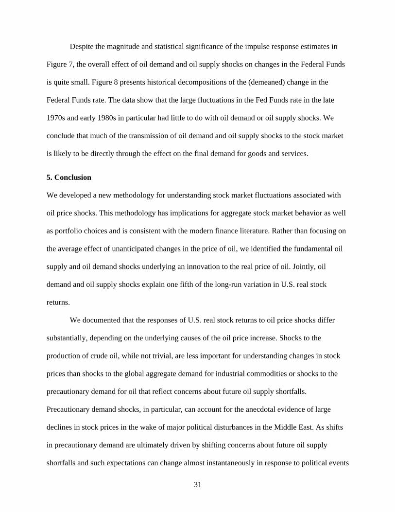
Despite the magnitude and statistical significance of the impulse response estimates in

Figure 7, the overall effect of oil demand and oil supply shocks on changes in the Federal Funds

is quite small. Figure 8 presents historical decompositions of the (demeaned) change in the

Federal Funds rate. The data show that the large fluctuations in the Fed Funds rate in the late

1970s and early 1980s in particular had little to do with oil demand or oil supply shocks. We

conclude that much of the transmission of oil demand and oil supply shocks to the stock market

is likely to be directly through the effect on the final demand for goods and services.

5. Conclusion

We developed a new methodology for understanding stock market fluctuations associated with

oil price shocks. This methodology has implications for aggregate stock market behavior as well

as portfolio choices and is consistent with the modern finance literature. Rather than focusing on

the average effect of unanticipated changes in the price of oil, we identified the fundamental oil

supply and oil demand shocks underlying an innovation to the real price of oil. Jointly, oil

demand and oil supply shocks explain one fifth of the long-run variation in U.S. real stock

returns.

We documented that the responses of U.S. real stock returns to oil price shocks differ

substantially, depending on the underlying causes of the oil price increase. Shocks to the

production of crude oil, while not trivial, are less important for understanding changes in stock

prices than shocks to the global aggregate demand for industrial commodities or shocks to the

precautionary demand for oil that reflect concerns about future oil supply shortfalls.

Precautionary demand shocks, in particular, can account for the anecdotal evidence of large

declines in stock prices in the wake of major political disturbances in the Middle East. As shifts

in precautionary demand are ultimately driven by shifting concerns about future oil supply

shortfalls and such expectations can change almost instantaneously in response to political events

32

in the Middle East, exogenous political disturbances may trigger an immediate and sharp

increase in precautionary demand that is reflected in an immediate jump in the real price of oil as

well as an immediate drop in stock prices. In contrast, if higher oil prices are driven by an

unanticipated global economic expansion, there will be persistent positive effects on cumulative

stock returns within the first year, as the stimulus emanating from a global business cycle

expansion initially outweighs the drag on the economy induced by higher oil prices. Our findings

both complement and reinforce the evidence in Kilian (2007a) about the response of U.S. real

GDP growth and consumer price inflation to demand and supply shocks in the crude oil market.

Our analysis suggests that the traditional approach to thinking about oil price changes and

stock prices must be rethought. An immediate implication of our analysis is that researchers have

to move beyond empirical and theoretical models that vary the price of oil while holding

everything else fixed. Relaxing this counterfactual ceteris paribus assumption helps resolve two

main puzzles in the related literature. First, it helps explain the apparent resilience of the U.S.

stock market to higher oil prices to date, given the evidence that recent increases in the price of

crude oil have been driven primarily by strong global demand for all industrial commodities. In

contrast, conventional VAR models based on unanticipated changes in the price of oil would

have mistakenly predicted a decline in the equity market in response to the most recent surge in

the price of oil. Second, our approach helps explain the apparent instability of regressions of

stock market variables on oil price changes. Such instabilities arise by construction from changes

in the composition of oil demand and oil supply shocks over time.

Using industry-level stock returns, we provided new evidence that the primary channel of

transmission of oil price shocks is a reduction in the final demand for goods and services. This

evidence is consistent with a growing body of evidence on the importance of the demand channel

(see, e.g., Lee and Ni 2002, Edelstein and Kilian 2007a,b). Our analysis has direct implications

33

for the construction of DSGE models of the link between oil prices and stock prices. We

highlighted the importance of, first, integrating the crude oil market into general equilibrium

models and, second, of modeling the U.S. and foreign demand for crude oil explicitly. This

contrasts sharply with the current generation of DSGE models such as Wei (2003) that postulate

an exogenous ARMA(1,1) process for oil prices and stress the effect of higher oil prices on

aggregate productivity.

References Alquist, R., and L. Kilian (2007), “What Do We Learn from the Price of Crude Oil Futures?” mimeo, Department of Economics, University of Michigan. Barsky, R. B., and L. Kilian (2002) “Do We Really Know that Oil Caused the Great Stagflation? A Monetary Alternative,” NBER Macroeconomics Annual 2001, 137-183. Barsky, R. B., and L. Kilian (2004) “Oil and the Macroeconomy since the 1970s,” Journal of Economic Perspectives, 18, 115-134. Bernanke, B.S., M. Gertler, and M.W. Watson (1997), “Systematic Monetary Policy and the

Effects of Oil Price Shocks,” Brookings Papers on Economic Activity, 1, 91-157. Bodenstein, M., C.J. Erceg, and L. Guerrieri (2007), “Oil Shocks and External Adjustment,”

mimeo, Federal Reserve Board.

Campbell, J.Y. (1991), “A Variance Decomposition for Stock Returns,” Economic Journal, 101, 157-179. Campbell, J.Y., and J.H. Cochrane (1999), “By Force of Habit: A Consumption-Based

Explanation of Aggregate Stock Market Behavior,” Journal of Political Economy, 107, 205-251.

Campbell, J.Y., Lo, A.W., and A.C. MacKinlay (1997), The Econometrics of Financial Markets, Princeton University Press: Princeton, NJ. Chen, N.-F., Roll, R., and S.A. Ross (1986), “Economic Forces and the Stock Market,” Journal of Business, 59, 383-403. Cochrane, J.H. (2005), Asset Pricing, 2nd ed., Princeton University Press: Princeton, NJ. Den Haan, W. J. (2000), “The Comovement between Output and Prices,” Journal of Monetary Economics, 46, 3-30.

34

Den Haan, W.J., and S.W. Summer (2004), “The Comovement between Real Activity and Prices in the G7,” European Economic Review, 48, 1333-1347. Dhawan, R., and K. Jeske (2006), “Energy Price Shocks and the Macroeconomy: The Role of

Consumer Durables,” Working Paper No. 2006-9, Federal Reserve Bank of Atlanta. Edelstein, P., and L. Kilian (2007a), “Retail Energy Prices and Consumer Expenditures,” mimeo, Department of Economics, University of Michigan. Edelstein, P., and L. Kilian (2007b), “The Response of Business Fixed Investment to Energy Price Changes: A Test of some Hypotheses about the Transmission of Energy Price Shocks,” B.E. Journal of Macroeconomics, 7 (Contributions), 1-39. Fama, E. F. (1981) “Stock Returns, Real Activity, Inflation and Money,” American Economic Review, 71, 545-565. Fama, E. F., and G. W. Schwert (1977) “Asset Returns and Inflation,” Journal of Financial Economics, 5, 115-146. Financial Times, “Equities Hit by Oil Rise and Geopolitical Angst”, August 21, 2006. Financial Times, “Oil Slide Spurs Global Equity Rally”, October 12, 2006. Gonçalves, S., and L. Kilian (2004), “Bootstrapping Autoregressions with Conditional Heteroskedasticity of Unknown Form,” Journal of Econometrics, 123, 89-120. Hamilton, J.D. (1988). “A Neoclassical Model of Unemployment and the Business Cycle,”

Journal of Political Economy. 96, 593-617. Hamilton, J.D. (2003) “What is an Oil Shock?” Journal of Econometrics, 113, 363-398. Hamilton, J.D. (2005), “Oil and the Macroeconomy,” forthcoming in: S. Durlauf and L. Blume

(eds.), The New Palgrave Dictionary of Economics, 2nd ed., London: Macmillan, 2006. Available at: http://dss.ucsd.edu/~jhamilto/JDH_palgrave_oil.pdf

Herrera, A.-M., and E. Pesavento (2007), “Oil Price Shocks, Systematic Monetary Policy, and the Great Moderation,” forthcoming: Macroeconomic Dynamics. Hess, P. J. and B. S. Lee (1999), “Stock Returns and Inflation with Supply and Demand Disturbances,” Review of Financial Studies, 12, 1203-1218. Huang, R., R. Masulis, and H. Stoll (1996), “Energy Shocks and Financial Markets,” Journal of Futures Markets, 16, 1-27. Jaffe, J. F., and G. Mandelker (1976), “The ‘Fisher Effect’ for Risky Assets: An Empirical

Investigation,” Journal of Finance, 31, 447-458. Jones, C., and G. Kaul (1996) “Oil and the Stock Markets,” Journal of Finance, 51, 463-491.

35

Kaul, G. (1987), “Stock Returns and Inflation: The Role of the Monetary sector,” Journal of Financial Economics, 18, 253-276. Kaul, G., and H.N. Seyhun (1990), “Relative Price Variability, Real Shocks and the

Stock Market,” Journal of Finance, 45, 479-496. Kilian, L. (2008a), “Exogenous Oil Supply Shocks: How Big Are They and How Much Do They Matter for the US Economy?” forthcoming: Review of Economics and Statistics.

Kilian, L. (2008b), “A Comparison of the Effects of Exogenous Oil Supply Shocks on Output And Inflation in the G7 Countries,” forthcoming: Journal of the European Economic Association. Kilian, L. (2007a) “Not All Oil Price Shocks Are Alike: Disentangling Demand and Supply Shocks in the Crude Oil Market,” mimeo, University of Michigan. Available at:

http://www-personal.umich.edu/~lkilian/paperlinks.html Kilian, L. (2007b), “The Economic Effects of Energy Price Shocks”, invited by the Journal of Economic Literature. Kling, J.L. (1985), “Oil Price Shocks and Stock-Market Behavior,” Journal of Portfolio

Management, 12, 34-39. Lee, K., and S. Ni (2002), “On the Dynamic Effects of Oil Price Shocks: A Study Using Industry Level Data,” Journal of Monetary Economics, 49, 823-852. Lettau, M., and S.C. Ludvigson (2005), “Expected Returns and Expected Dividend Growth,” Journal of Financial Economics, 76(3), 583-626. Nakov, A., and A. Pescatori (2007), “Inflation-Output Gap Trade-off with a Dominant Oil

Supplier,” mimeo, Federal Reserve Bank of Cleveland. New York Times, “Retail Sales Slow as Jobless Claims Drop”, September 14, 2006. Sadorsky, P. (1999), “Oil Price Shocks and Stock Market Activity,” Energy Economics, 21, 449- 469. Torous, W., R. Valkanov, and S. Yan (2005) “On Predicting Stock Returns with Nearly Integrated Explanatory variables,” Journal of Business, 77, 937-966. Wei, C. (2003) “Energy, the Stock Market, and the Putty-Clay Investment model,” American Economic Review, 93, 311-323.

Table 1: Percent Contribution of Demand and Supply Shocks in the Crude Oil Market to

the Overall Variability of U.S. Real Stock Returns

Horizon Oil Supply Shock

Aggregate Demand Shock

Oil-specific Demand Shock

Other Shocks

1 0.06 0.02 1.37 98.55 2 0.08 0.50 4.66 94.76 3 0.30 0.72 5.26 93.72 12 1.53 2.60 6.81 89.07 ∞ 6.40 5.13 10.51 77.96

NOTES: Based on variance decomposition of the structural VAR model (1).

Table 2: Percent Contribution of Demand and Supply Shocks in the Crude Oil Market to

the Overall Variability of U.S. Real Dividend Growth

Horizon Oil Supply

Shock Aggregate Demand Shock

Oil-specific Demand Shock

Other Shocks

1 0.20 0.16 1.69 97.95 2 0.55 0.36 2.09 97.00 3 0.76 0.48 2.12 96.64 12 2.80 6.83 4.53 85.84 ∞ 6.63 8.38 7.93 77.06

NOTES: Based on variance decomposition of the structural VAR model (1)

with U.S. real dividend growth included instead of U.S. real returns.

Table 3: Tests of the Impact Response of U.S. Real Stock Returns Wald test statistic

36

0 00

: , 1,2,3ij ij

i

H jψ ρ δ=

= =∑

p -value

Oil supply shocks 2.5017 0.1137 Aggregate demand shocks 1.6678 0.1966 Oil-market specific demand shocks

0.8888 0.3458

Wald test statistic

36

0 01

: , 1,2,3ij ij

i

H jψ ρψ=

= − =∑p -value

Oil supply shocks 0.0150 0.9024 Aggregate demand shocks 0.0935 0.7598 Oil-market specific demand shocks

1.2840 0.2572

Notes: ijψ denotes the response of real stock returns i periods after shock 1,2,3j = occurred.

ijδ denotes the corresponding response of real dividend growth. The first test is for the null

hypothesis that the contemporaneous return response is fully explained by changes in expected

dividend growth; the second test is for the null hypothesis that the contemporaneous return

response is fully explained by fluctuations in expected returns. All p-values were computed

based on a recursive-design wild bootstrap.

0 5 10 15-6

-4

-2

0

2

4

6

8

10

12Oil supply shock

Rea

l pric

e of

oil

Months0 5 10 15

-6

-4

-2

0

2

4

6

8

10

12Aggregate demand shock

Rea

l pric

e of

oil

Months0 5 10 15

-6

-4

-2

0

2

4

6

8

10

12Oil-specific demand shock

Rea

l pric

e of

oil

Months

Figure 1: Responses of the Real Price of Crude Oil to One-Standard Deviation Structural Shocks Point Estimates with One- and Two-Standard Error Bands

NOTES: Estimates based on the VAR model described in text. The confidence intervals were constructed using a recursive- design wild bootstrap (see Gonçalves and Kilian 2004).

1980 1985 1990 1995 2000 2005-100

-50

0

50

100Cumulative Effect of Oil Supply Shock on Real Price of Crude Oil

1980 1985 1990 1995 2000 2005-100

-50

0

50

100Cumulative Effect of Aggregate Demand Shock on Real Price of Crude Oil

1980 1985 1990 1995 2000 2005-100

-50

0

50

100Cumulative Effect of Oil-Market Specific Demand Shock on Real Price of Crude Oil

Figure 2: Historical Decomposition of Real Price of Oil 1975.1-2006.12

NOTES: Estimates based on VAR model described in text.

0 5 10 15-3

-2

-1

0

1

2

3Oil supply shock

Cum

ulat

ive

Rea

l Sto

ck R

etur

ns (P

erce

nt)

0 5 10 15-3

-2

-1

0

1

2

3Aggregate demand shock

Cum

ulat

ive

Rea

l Sto

ck R

etur

ns (P

erce

nt)

0 5 10 15-3

-2

-1

0

1

2

3Oil-specific demand shock

Cum

ulat

ive

Rea

l Sto

ck R

etur

ns (P

erce

nt)

0 5 10 15-3

-2

-1

0

1

2

3Oil supply shock

Cum

ulat

ive

Rea

l Div

iden

ds (P

erce

nt)

Months0 5 10 15

-3

-2

-1

0

1

2

3Aggregate demand shock

Cum

ulat

ive

Rea

l Div

iden

ds (P

erce

nt)

Months0 5 10 15

-3

-2

-1

0

1

2

3Oil-specific demand shock

Cum

ulat

ive

Rea

l Div

iden

ds (P

erce

nt)

Months

Figure 3: Cumulative Reponses of U.S. Real Stock Returns and Real Dividend Growth Point Estimates with One- and Two-Standard Error Bands

NOTES: Estimates based on the VAR model described in text. The confidence intervals were constructed using a recursive-design wild bootstrap (see Gonçalves and Kilian 2004).

0 5 10 15-3

-2

-1

0

1

2

3Real oil price shock

Cum

ulat

ive

Rea

l Sto

ck R

etur

ns (P

erce

nt)

Months

Figure 4: Cumulative Responses of U.S. Real Stock Returns to Real Oil Price Innovation Point Estimates with One- and Two-Standard Error Bands

NOTES: Estimates based on the VAR model described in text. The confidence intervals were constructed using a recursive- design wild bootstrap (see Gonçalves and Kilian 2004).

0 5 10 15-0.1

-0.08

-0.06

-0.04

-0.02

0

0.02

0.04

Oil supply shock

0 5 10 15-0.1

-0.08

-0.06

-0.04

-0.02

0

0.02

0.04

Aggregate demand shock

0 5 10 15-0.1

-0.08

-0.06

-0.04

-0.02

0

0.02

0.04

Oil-specific demand shock

Months

Figure 5: Conditional Covariance between Responses of U.S. Real Stock Returns and Inflation Point Estimates with 90% Confidence Bands

NOTES: Estimates based on VAR models described in text. The confidence intervals were constructed using a recursive-design wild bootstrap (see Gonçalves and Kilian 2004).

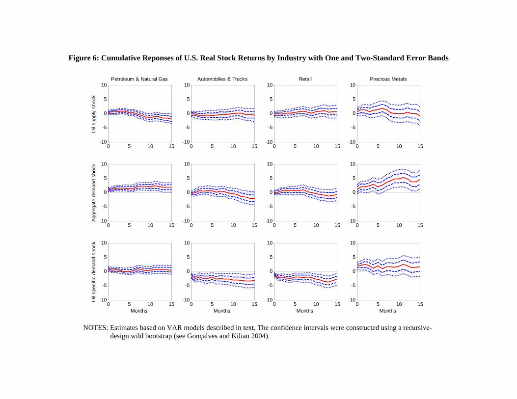
0 5 10 15-10

-5

0

5

10Petroleum & Natural Gas

Oil

supp

ly s

hock

0 5 10 15-10

-5

0

5

10

Agg

rega

te d

eman

d sh

ock

0 5 10 15-10

-5

0

5

10

Oil-

spec

ific

dem

and

shoc

k

Months

0 5 10 15-10

-5

0

5

10Automobiles & Trucks

0 5 10 15-10

-5

0

5

10

0 5 10 15-10

-5

0

5

10

Months

0 5 10 15-10

-5

0

5

10Retail

0 5 10 15-10

-5

0

5

10

0 5 10 15-10

-5

0

5

10

Months

0 5 10 15-10

-5

0

5

10Precious Metals

0 5 10 15-10

-5

0

5

10

0 5 10 15-10

-5

0

5

10

Months

Figure 6: Cumulative Reponses of U.S. Real Stock Returns by Industry with One and Two-Standard Error Bands

NOTES: Estimates based on VAR models described in text. The confidence intervals were constructed using a recursive- design wild bootstrap (see Gonçalves and Kilian 2004).

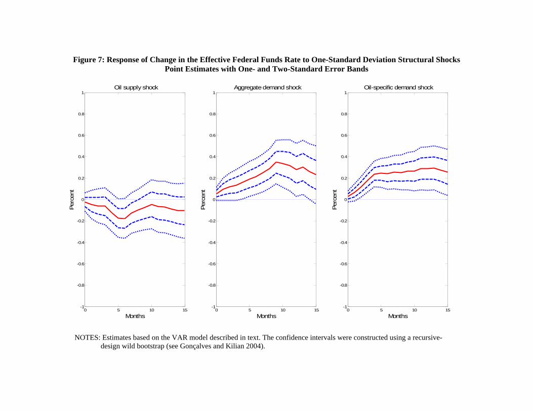
0 5 10 15-1

-0.8

-0.6

-0.4

-0.2

0

0.2

0.4

0.6

0.8

1Oil supply shock

Perc

ent

Months0 5 10 15

-1

-0.8

-0.6

-0.4

-0.2

0

0.2

0.4

0.6

0.8

1Aggregate demand shock

Perc

ent

Months0 5 10 15

-1

-0.8

-0.6

-0.4

-0.2

0

0.2

0.4

0.6

0.8

1Oil-specific demand shock

Perc

ent

Months

Figure 7: Response of Change in the Effective Federal Funds Rate to One-Standard Deviation Structural Shocks Point Estimates with One- and Two-Standard Error Bands

NOTES: Estimates based on the VAR model described in text. The confidence intervals were constructed using a recursive- design wild bootstrap (see Gonçalves and Kilian 2004).

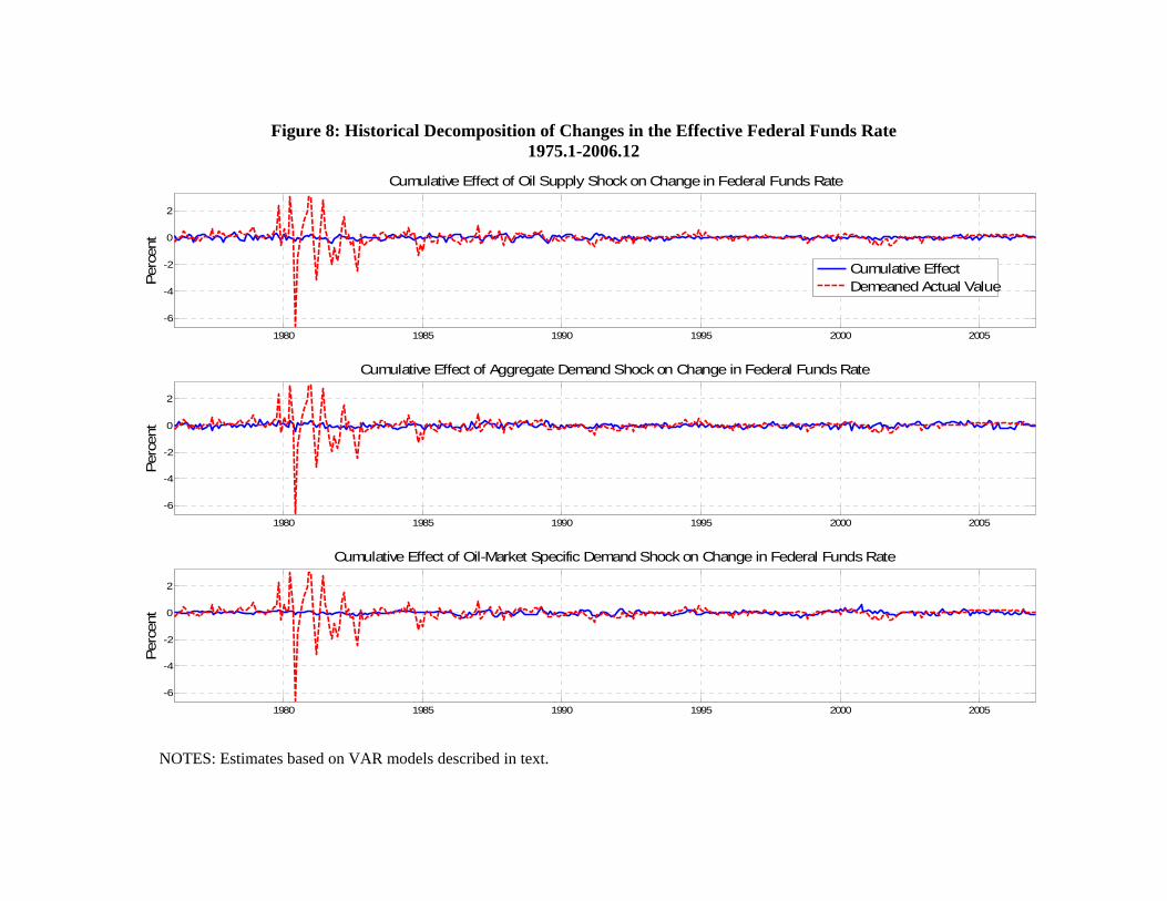
1980 1985 1990 1995 2000 2005

-6

-4

-2

0

2

Cumulative Effect of Oil Supply Shock on Change in Federal Funds Rate

Perc

ent

Cumulative EffectDemeaned Actual Value

1980 1985 1990 1995 2000 2005

-6

-4

-2

0

2

Cumulative Effect of Aggregate Demand Shock on Change in Federal Funds Rate

Perc

ent

1980 1985 1990 1995 2000 2005

-6

-4

-2

0

2

Cumulative Effect of Oil-Market Specific Demand Shock on Change in Federal Funds Rate

Perc

ent

Figure 8: Historical Decomposition of Changes in the Effective Federal Funds Rate 1975.1-2006.12

NOTES: Estimates based on VAR models described in text.