DI

SC

US

SI

ON

P

AP

ER

S

ER

IE

S

Forschungsinstitut zur Zukunft der ArbeitInstitute for the Study of Labor

The Impact of Non-Parental Child Care onChild Development: Evidence from theSummer Participation “Dip”

IZA DP No. 7039

November 2012

Chris M. Herbst

The Impact of Non-Parental Child Care on Child Development: Evidence from

the Summer Participation “Dip”

Chris M. Herbst Arizona State University

and IZA

Discussion Paper No. 7039 November 2012

IZA

P.O. Box 7240 53072 Bonn

Germany

Phone: +49-228-3894-0 Fax: +49-228-3894-180

E-mail: iza@iza.org

Any opinions expressed here are those of the author(s) and not those of IZA. Research published in this series may include views on policy, but the institute itself takes no institutional policy positions. The IZA research network is committed to the IZA Guiding Principles of Research Integrity. The Institute for the Study of Labor (IZA) in Bonn is a local and virtual international research center and a place of communication between science, politics and business. IZA is an independent nonprofit organization supported by Deutsche Post Foundation. The center is associated with the University of Bonn and offers a stimulating research environment through its international network, workshops and conferences, data service, project support, research visits and doctoral program. IZA engages in (i) original and internationally competitive research in all fields of labor economics, (ii) development of policy concepts, and (iii) dissemination of research results and concepts to the interested public. IZA Discussion Papers often represent preliminary work and are circulated to encourage discussion. Citation of such a paper should account for its provisional character. A revised version may be available directly from the author.

IZA Discussion Paper No. 7039 November 2012

ABSTRACT

The Impact of Non-Parental Child Care on Child Development: Evidence from the Summer Participation “Dip”1

Although a large literature examines the effect of non-parental child care on preschool-aged children’s cognitive development, few studies deal convincingly with the potential endogeneity of child care choices. Using a panel of infants and toddlers from the Birth cohort of the Early Childhood Longitudinal Study (ECLS-B), this paper attempts to provide causal estimates by leveraging heretofore unrecognized seasonal variation in child care participation. Child assessments in the ECLS-B were conducted on a rolling basis throughout the year, and I use the participation “dip” among those assessed during the summer as the basis for an instrumental variable. The summer participation “dip” is likely to be exogenous because ECLS-B administrators strictly controlled the mechanism by which children were assigned to assessment dates. The OLS results show that children utilizing non-parental arrangements score higher on tests of mental ability, a finding that holds after accounting for individual fixed effects. However, the instrumental variables estimates point to sizeable negative effects of non-parental care. The adverse effects are driven by participation in formal settings, and, contrary to previous research, I find that disadvantaged children do not benefit from exposure to non-parental child care settings. JEL Classification: J13 Keywords: child care, child development, maternal employment Corresponding author: Chris M. Herbst School of Public Affairs Arizona State University 411 N. Central Ave., Suite 480 Phoenix, AZ 85004-0687 USA E-mail: chris.herbst@asu.edu

1 I am grateful to participants at the 2012 meeting of the Association for Public Policy Analysis and Management and Southern Economic Association, as well as Joanna Lucio, Erdal Tekin, Bob Bradley, Greg Duncan, Spiro Maroulis, Anna Johnson, Nikki Forry, Melanie Guldi and Joseph Doyle for helpful comments and suggestions.

2

I. Introduction

Over the past few decades, there has been a sharp increase in the share of U.S. preschool-

aged children participating non-parental child care arrangements. Currently, two-thirds of young

children regularly attend some form of child care, with the average child spending 32 hours per week

in these settings (Laughlin, 2010). Moreover, the transition into non-parental care occurs rapidly after

childbirth. According to the NICHD Study of Early Child Care (1997a), the typical child first enters

child care at approximately three months. Within the first year of life, 80 percent experience regular

participation in non-parental arrangements, and over one-third have at least three distinct caregivers.

The most common child care setting for preschool-aged children is relative care (41 percent),

followed by center- (23 percent) and family-based (13 percent) arrangements (Laughlin, 2010).

Catalyzed by the finding that early childhood health (e.g., Almond & Currie, 2010; Case et

al., 2005) and educational experiences (e.g., Heckman & Materov, 2007; Karoly et al., 2005) may

have lasting effects on schooling and labor market success, developmental psychologists and

economists have devoted significant attention to studying the impact of various child care

arrangements on child development. Recent work examines a variety of outcomes, ranging from the

incidence of injury and infectious disease to cognitive and social-emotional functioning. Although

results from this work are quite mixed overall, two themes consistently emerge (Bradley & Vandell,

2007; Pianta et al., 2009). First, participation in center-based care has opposing effects child

development, producing small improvements in mental ability test scores while increasing behavior

problems. Second, higher-quality settings produce more favorable short- and long-run outcomes,

especially for economically disadvantaged children.

An important concern with much of this research is the insufficient attention paid to the

potential endogeneity of child care choices. Families using non-parental arrangements are likely to

differ from those that do not in ways that cannot be fully accounted for even in richly specified child

production functions. If these unobserved differences are correlated with measures of child

3

development, a classic case of omitted variable bias arises, in which the estimated effect of non-

parental care is confounded. To date, only a small number of U.S. studies attempt to handle these

identification issues. One paper makes use of value-added specifications (NICHD ECCRN &

Duncan, 2003), another three use fixed effects (Blau, 1999; Currie & Hotz, 2004; Gordon et al.,

2007), and one implements an instrumental variables strategy (Bernal & Keane, 2011).2 The latter

paper is noteworthy because it finds that increased child care time during the preschool years reduces

mental ability test scores, a result at odds with much of the OLS literature. Therefore, considerable

uncertainty remains over the implications of non-parental child care utilization for children’s

development.

Using a panel of infants and toddlers from the Birth cohort of the Early Childhood

Longitudinal Study (ECLS-B), this paper provides new evidence on the impact of non-parental child

care utilization on mental ability test scores. To distinguish between short- and longer-run effects, the

analysis considers two measures of child care utilization. It begins by examining an indicator of

current participation in any non-parental arrangement, followed by finer comparisons of formal and

informal arrangements as well as relative, non-relative, and center-based settings. It then focuses on

cumulative child care utilization, defined as the number of months a given focal child participated in

non-parental arrangements at each assessment point. The primary contribution of the paper is the use

of a novel empirical strategy to estimate the causal effect of non-parental care. Specifically, it

exploits heretofore unrecognized seasonal patterns in child care utilization to provide identifying

variation. During the first two waves of the ECLS-B, parental interviews and child assessments were

conducted on a rolling basis throughout the year, and I use the child care participation “dip” that

occurred among those assessed during the summer as the basis for an instrumental variable. The

2 Note that these papers explore the first-order question of the impact of various non-parental child care arrangements on child development. This topic is distinct from, although related to, the second-order question of the impact of various child care and early education policies (e.g., Child Care and Development Fund, Head Start, and pre-kindergarten) on child development. Generally speaking, obtaining credible identification strategies has been more difficult for studies pursuing the former question than the latter.

4

estimated summer-induced drop in utilization is strong in the first-stage equation, and it pervades

most demographic sub-groups, including working and non-working mothers.

I argue that the timing of ECLS-B assessments generates exogenous variation in child care

utilization because parents were not given the opportunity to choose an assessment date. Instead,

since the survey was designed to document age-specific developmental milestones, ECLS-B

administrators assigned parents to interview dates based on the focal child’s birthday. Interviews for

the first wave were initiated at the child’s 9-month birthday, while those for the second wave

occurred at 24- months. I show that families overwhelmingly complied with this assignment rule, and

I provide evidence that families interviewed during the summer are observationally equivalent to

their counterparts interviewed during other times of the year. Importantly, there is no indication that

parents’ employment status differs across the summer and non-summer months, nor is there evidence

of seasonality in the demand for child care quality, underlying child health, or maternal mental

health. Given that the assignment mechanism is based on the focal child’s birthday, one concern is

that unobserved family differences associated with season-of-birth might invalidate the summer

assessment instrument. Indeed, Buckles and Hungerman (2010) document strong seasonal patterns in

the socioeconomic characteristics of women giving birth throughout the year. Fortunately, the

identification strategy does not require quarter-of-birth to be excluded from the child production

function, and the instrumental variables estimates are robust to the inclusion of such controls.

The paper’s main findings can be summarized as follows. I first show that children attending

non-parental care are more economically advantaged than their peers in parent care. This positive

selection suggests that OLS estimates of child care utilization are likely to be biased upward. I then

recreate the standard OLS result in the literature that children attending non-parental care score

higher on tests of early mental ability, a result that holds when I account for individual fixed effects.

However, the instrumental variables estimates point to sizeable negative effects of non-parental child

care utilization. For example, baseline results for the measure of current child care participation

5

suggest that ability test scores are 8.5 percent to 9.5 percent lower for children in non-parental

settings, corresponding to an effect size of approximately 0.29 standard deviations. Contrary to

previous research, the negative effects are driven by participation in formal care—including center-

based and non-relative arrangements—and I show that disadvantaged children do not benefit from

exposure to non-parental settings.

The remainder of the paper proceeds as follows. The next section summarizes previous

research examining the relationship between early non-parental care and child development. Section

III introduces the key features of the ECLS-B analysis sample, and Section IV develops the

identification strategy. The estimation results are presented in Section V, while Section VI concludes

with a discussion of policy implications.

II. Relevant Literature

There is a voluminous literature in developmental psychology and, increasingly, economics

examining the relationship between non-parental child care arrangements and child development.3

The intent here is to provide an overview of the most relevant work, focusing on the short-run effects

of infant and toddler care on four of the most heavily studied outcomes: the mother-child

relationship, injuries and communicable illnesses, behavior problems, and mental ability.

The early mother-child relationship is widely considered the foundation of children’s later

psychological and mental development (Collins et al., 2000).4 Initial research therefore focused on

whether the early and intense use of non-parental care disrupts this relationship (Belsky & Steinberg,

1978). For example, it is possible that prolonged separation limits mothers’ ability respond

sensitively to the child, while reducing the child’s confidence in the availability and consistency of

maternal responsiveness. The most recent empirical evidence indicates that routine non-parental care,

3 Comprehensive reviews are found in Bernal and Keane (2011), Bradley and Vandell (2007), and Pianta et al. (2009). 4 Indeed, a range of parenting practices from spanking and psychological aggression to the level of maternal sensitivity are found to directly influence children’s cognitive and behavioral well-being (Gershoff, 2002; Ispa et al., 2002).

6

particularly in the first year of life, is associated with elevated rates of attachment insecurity (NICHD

ECCRN, 1997b; 2001a) and reduced maternal sensitivity (NICHD ECCRN, 1999).

Previous work also explores the link between non-parental care and rates of injury and

communicable illnesses. It is conceivable that early entry into child care, especially settings with

large group sizes, increases the likelihood of exposure to pathogens carried by other children. The net

effect of prolonged child care exposure could be zero, however, as children beginning non-parental

care early in life might develop immunities that prevent the onset of illness during the school-age

years. Nevertheless, given the large social costs of treating early childhood injury and illness

(Auinger et al., 2003), and the potential long-term impact of early health status (Case et al., 2002), a

number of studies examine whether certain child care arrangements are responsible for catalyzing

adverse health events. This work consistently finds that time spent in center-based, and to a lesser

extent family-based, settings is associated with a greater risk of contracting respiratory and ear

infections but not with incurring serious injuries (Gordon et al., 2007; NICHD ECCRN 2001b;

2003a). These effects largely disappear by the time children reach 36-months—indicative of the

immunizing effects of early exposure—and there are no detectable spillovers to other areas of child

development.

The third domain of research considers children’s behavioral development, including positive

peer interactions, self-control, and compliance. Such skills are critical to early school achievement

and are shown to have long-run implications for mental and behavioral functioning (Raver, 2002).

Results from the NICHD ECCRN (1998; 2001c; 2003b) reveal that non-parental care is associated

with poorer peer interactions and increased behavior problems, with earlier entry and more intense

exposure magnifying the negative effects and higher-quality settings mollifying them. Greater

exposure to center-based care in particular increases early disruptive behavior that persists

throughout childhood (Belsky et al., 2007). Similar results are evident in other U.S. datasets,

including the National Longitudinal Survey of Youth (NLSY) (Bernal & Keane, 2011).

7

The most relevant cluster of research focuses on the implications of early non-parental care

for children’s mental development. Overall, results from this work tend to find beneficial effects of

child care exposure (NICHD ECCRN, 2000), although some uncover neutral (Blau, 1999) or

negative effects (Bernal & Keane, 2011; NICHD ECCRN, 2004). There is a growing consensus,

however, that high-quality center-based settings produce favorable results (Hill et al., 2002; NICHD

ECCRN & Duncan, 2003; Peisner-Feinberg et al., 2001), especially when child care teachers engage

in cognitively stimulating interactions with children (NICHD ECCRN, 2000). The positive effects of

early center-based care tend to be larger for economically disadvantaged children (Loeb et al., 2004),

and they are found to persist throughout the school-aged years (Belsky et al., 2007).

Despite this extensive literature, most papers do not deal adequately with the potential

endogeneity of child care choices. The most common strategy is to estimate the child production

function using ordinary least squares (OLS) regression, conditioning on a rich set of observable

family characteristics. However, OLS estimates of child care utilization may still be inconsistent

because families using child care may differ from those that do not in ways that are difficult to

capture. For example, families using non-parental care may have stronger work preferences, face

fewer constraints on obtaining work and child care, or place a higher value on socializing children at

an early age. In addition, children exposed to non-parental care may have qualities that parents wish

to enhance (e.g., high mental ability) or ameliorate (e.g., disabilities). In other words, child well-

being could itself be a determinant of parental child care decisions. Failure to account for these

systematic differences across families and children will yield inconsistent estimates of the impact of

non-parental child care utilization.

To my knowledge, only a few studies attempt to handle these identification problems. One

paper makes use of value-added specifications (NICHD ECCRN & Duncan, 2003), another three use

fixed effects (Blau, 1999; Currie & Hotz, 2004; Gordon et al., 2007), and one implements an

8

instrumental variables (IV) strategy (Bernal & Keane, 2011).5 Identification in value-added models is

achieved by conditioning on pre-child-care-use (or lagged) mental ability, which is assumed to

capture the child’s ability endowment as well as unobserved historical inputs. However, as Todd and

Wolpin (2003) show, endogeneity problems arise when lagged mental ability is correlated with the

unobserved contemporaneous determinants of ability.6 The primary advantage of the individual fixed

effects model is that it compares a child’s mental ability in periods of child care exposure with the

ability of the same child in periods of non-exposure. Although this within-child estimator accounts

for time-invariant unobservables, a concern is that omitted time-varying inputs will still lead to

inconsistent estimates.

The paper by Bernal and Keane (2011) represents the only other attempt to use IV methods in

the child care-child development literature. The identification strategy uses 78 social policy variables

(e.g., welfare reform rules) to instrument for child care time in a sample of single mothers from the

NLSY. The paper’s main finding is that each year of child care exposure reduces preschool-aged

children’s mental ability test scores by 2.1 percent, with participation in informal care driving the

negative effects. Although the policy instruments are reasonably powerful in the first-stage equation

(F=14.7), it is possible that many of them are related to child development beyond their correlation

with child care time, thus potentially invalidating them as instruments.7 Another concern is that the

measure of child care time is derived from mothers’ employment history, making it difficult to

5 The claim that only one other child care paper utilizes an IV strategy should not be confused with the work of Gelbach (2002) and Herbst and Tekin (2010a; 2012). Gelbach instruments for kindergarten attendance, not child care arrangements per se, and explores maternal employment as the outcome. The Herbst and Tekin papers instrument for child care subsidy receipt, again not arrangements per se, but they do examine various measures of child health and development. The paper by Bernal and Keane (2011) represents the only other attempt to instrument for preschool non-parental child care arrangements, a task made very difficult because of a death of variation in child care decisions that is not correlated with maternal employment decisions. 6 For example, parents in the current period may engage in optimizing behavior in response to child well-being in previous periods. 7 For example, one of the authors’ instruments, state-level child enforcement expenditures, is likely to change the behavior of children’s biological fathers in ways that affect child well-being (e.g., through increased time investments). Welfare policies such as child-age-exemptions from work requirements may influence women’s fertility decisions, and therefore optimizing behavior regarding quality-quantity trade-offs in maternal investments. Moreover, welfare work requirements and time limits can conceivably influence family well-being in ways that are unrelated to child care and work decisions (e.g., through changes in the home environment). Finally, local labor market conditions are known to affect individual health through non-labor-market mechanisms (e.g., through changes in consumption and health-related behaviors).

9

separately identify the impact of child care exposure and maternal employment.8 The current paper

builds on Bernal and Keane (2011) by introducing a new instrument to produce credible estimates of

the impact of non-parental child care arrangements. The strategy developed here is advantageous

because it exploits the ECLS-B’s birthday-based assessment schedule, a design feature that is

replicated in other surveys of children’s early child care experiences (e.g., Fragile Families and Child

Well-Being Study). Thus, future work can exploit this identification strategy to examine other child

development outcomes.

III. Data

Data for this research are drawn from the Birth cohort of the Early Childhood Longitudinal

Study (ECLS-B), a nationally representative sample of approximately 11,000 children born in 2001.9

The survey was designed to track children’s early home and educational experiences by conducting

detailed parent and child care provider interviews and initiating a battery of child assessments at

various points between birth and kindergarten entry. The first wave of data collection occurred when

focal children were 9-months-old (2001-2002), with follow-up surveys implemented at 24-months

(2003), during the preschool year (2005-2006), and after kindergarten entry (2006-2007).

The analysis sample is a panel of children from the 9- and 24-month waves of data collection,

during which direct child assessments were administered and parents completed detailed

questionnaires. In particular, trained interviewers conducted a home visit on or near the focal child’s

9- and 24-month birthday. The home visit consisted of child mental and psychomotor assessments

and a 60-minute parent interview to ascertain information about demographic and labor market

8 Indeed, one of the reasons the authors are able to leverage reasonably good explanatory power in the first-stage is that the measure of child care time is closely linked to maternal employment, and polices such welfare reform and the EITC have had large effects on single mothers’ employment. This is problematic because early maternal employment itself has implications for child development (Brooks-Gunn et al., 2002; Ruhm, 2004; Morrill, 2011). 9 Children were sampled from birth registers from the National Center for Health Statistics (NCHS) vital statistics system. Births were sampled within a set of primary sampling units (PSUs) as well as secondary sampling units (SSUs). The original sample included approximately 14,000 births, 10,688 of whom had a completed assessment at the 9-month wave of data collection. The sampling frame included all births, with the following exceptions: children born to mothers less than 15 years-old; children who died prior to the 9-month assessment; and children who were adopted prior to the 9-month assessment. Several groups were oversampled, including low birth weight children, twins, and Native American children.

10

characteristics, the home environment, child and family health, and current child care utilization.10

Exclusions from the sample are made if a child is missing information on the month-of-assessment

(1,930) or the type of non-parental child care utilized (30). I retain children with at least one non-

missing mental ability test score from the 9- and 24-month assessments. The result is an unbalanced

panel of 10,477 children, providing 19,416 child-wave combinations.

The primary outcome is a measure of children’s early mental ability from the Bayley Short

Form—Research Edition (BSF-R) test. This instrument was designed specifically for the ECLS-B

and includes a subset of items from the full Bayley Scales of Infant Development—Second Edition

(BSID-II), a widely used measure of mental development from birth to preschool. Although the

original 178-item BSID-II was designed to be completed in a clinical setting, the BSF-R was

developed for ease of administration and completion in a home environment. The abbreviated 9- and

24-month BSF-R contains 31 and 33 mental items, respectively. The test assesses several dimensions

of early cognitive and language ability, including memory, preverbal communication, expressive and

receptive vocabulary, reasoning and problem solving, and concept attainment. Item response theory

(IRT) scale scores are used in the analysis.

This study examines two measures of non-parental child care utilization. To capture the

short-run effect of child care, I begin with a measure of current participation in any non-parental

arrangement. Specifically, I create a binary indicator that equals unity if a given child receives—at

the time of assessment—regular care from relatives (inside or outside the focal child’s home), non-

relatives (e.g., friends, neighborhoods, nannies, or family-based care inside or outside the focal

child’s home), and center-based services (e.g., nursery or preschools, for-profit centers, or non-profit

church organizations). Auxiliary analyses explore more nuanced measures of child care settings, in

particular, by comparing informal and formal child care arrangements as well as relative, non-

10 As stated in the text, parental interviews and child assessments were conducted at the same time during the home visit. For expositional ease, I will hereafter refer only to “child assessments” when discussing the bundle of family activities carried out by ECLS-B administrators during the home visit.

11

relative, and center-based settings.11 I then examine the longer-run effect of child care by

constructing a measure of cumulative participation in all non-parental arrangements, defined as the

total number of months of participation at each assessment date. To construct this measure, I

combine information on the age (in months) at which focal children began their first child care spell

with information on contemporaneous participation at the 9- and 24-month surveys.

The child production function also includes a rich set of child and family characteristics that

may be correlated with non-parental child care decisions and children’s mental ability. The vector of

child controls includes gender, age (up to a quartic polynomial), race and ethnicity (four dummy

variables), low birth weight (one dummy variable), premature birth (one dummy variable), and

weight (in kilograms). Parental skill and time inputs are proxied by mother’s age (up to a squared

polynomial), marital status (four dummy variables), maternal education (three dummy variables), the

presence of other children in the household (three dummy variables), maternal employment status

(three dummy variables), total household income (12 dummy variables), and urban residence (one

dummy variable).12 The model also includes state fixed effects.

Table 1 presents summary statistics for the analysis sample. Not surprisingly, the average

score on the BSF-R increases substantially from the 9- to the 24-month assessment (74.8 versus

125.5). Children receiving non-parental care at 9-months score one-point higher than their

counterparts in parent care, a test score gap that grows to approximately two-points by the 24-month

assessment. Tests of the null hypothesis of no test score differences are easily rejected at both

assessment points. Children in non-parental and parental care are equally likely to be male, white,

and classified as low birth weight or premature. However, a number of differences emerge across the

family characteristics. In particular, there is consistent evidence that children attending non-parental

11 Informal settings include relative care in any home and non-relative care in the focal child’s home. Formal settings are defined as non-relative care outside the child’s home (i.e., family-based services) and all forms of center-based care. In all cases, the omitted category includes children in parent care. 12 Missing data on child and family variables are retained by imputing zeroes for the missing values and creating dummy variables (that equal unity for the missing data) to account for the possibility of non-random imputation.

12

care are more advantaged than their peers in parent care. The former group is less likely to have

mothers who did not complete high school and more likely to have mothers who completed at least a

bachelor’s degree. Maternal employment rates are considerably higher among children attending

non-parental care, and household income is approximately 25 percent greater, on average. In

addition, children attending non-parental care are more likely to be an only-child, whereas those in

parent care are more likely to have three or more siblings (14.7 percent versus 8.1 percent,

respectively). Such comparisons are useful because they indicate the potential direction of the OLS

bias in the estimated effect of non-parental care. In particular, it appears that children receiving non-

parental care are positively selected, suggesting that the OLS estimates are biased upward.

Table 2 provides information on children’s participation in non-parental arrangements over

the infant and toddler years. Panel A shows the participation rate and weekly hours of participation

for the measure of current non-parental child care utilization; Panel B provides this information

disaggregated by informal and formal care; and Panel C shows data on cumulative participation.

Consistent with previous work, children in the ECLS-B experience intensive non-parental care early

in life: nearly half spend time in any arrangement as of the 9- and 24-month assessments, and they

are engaged in these settings for approximately 33 hours per week. The use of informal care becomes

less common as children age, while formal care becomes more common. Approximately 19 percent

of children experience a formal non-parental arrangement at 9-months, rising to 27 percent at 24-

months. The increased reliance on formal care is largely driven by growing participation in center-

based settings. Finally, Table 2 shows that children accumulate about four months of child care

exposure by their 9-month birthday, and 11 months of exposure by their 24-month birthday.

IV. Empirical Framework

Basic Estimation Strategy: OLS and Individual Fixed Effects Models

The empirical models described below are based on the Becker (1965) and Leibowitz (1974)

theoretical frameworks in which the household is assumed to be a productive unit that makes

13

decisions about the allocation of time and material resources. These decisions are aimed at

maximizing a household utility function of the form U(T, A, G; x1, x2,…,xn), where T represents

maternal time in leisure; A is a latent measure of child quality (or ability); G captures a set of goods

and services that enhance family well-being; and x is a series of exogenous preference shifters. This

study is concerned with the estimation of the household demand for child quality, A, which, in its

most general form, can be specified through the following cognitive ability production function:

(1) Ait = β1Tit + β2Cit + β3Git + Z′β + µit, where

T represents maternal time inputs (parental child care) for the ith child in each period, t; C is a

measure of time spent outside of maternal care (non-parental child care); Z′ is a matrix of observable

child and family characteristics related to the child’s ability endowment; and µ captures the

unobserved time invariant and time varying determinants of child ability. Note that maternal and

non-maternal time inputs, T and C, could enter the production function multiplicatively with quality,

such that the contribution of maternal and non-maternal time depends on the quality of that time.

As others note, a number of data and conceptual challenges make it infeasible to estimate

equation (1) in practice (e.g., Bernal & Keane, 2011; Todd & Wolpin, 2007). First, the inputs to child

ability are assumed to be measured in each period, and are thought to have period-specific effects on

the development pathway. To avoid the large number of variables necessary to support such a model,

most papers in the child development literature make the simplifying assumption inputs have

contemporaneous or cumulative effects on child ability. Another challenge is that maternal and non-

maternal time inputs are not measured directly in most survey datasets.13 A common approach is to

proxy for missing time inputs using indicator variables for maternal employment and non-parental

child care utilization. Such controls, however, do not account for the level of quality in maternal and

non-maternal time. Indeed, data exigencies preclude measuring the amount of time mothers spend 13 It is also the case G (e.g., the number of books in the home, access to cognitively stimulating toys and activities, access to and type of health insurance, and access to healthy food) are not observed directly in most survey datasets. To sidestep the problem, most studies enter household income into the production function. This variable is problematic for at least two reasons. First, it is endogenous. Second, it is a function of T and C, making it difficult to distinguish between the contribution of time inputs and material investments.

14

reading to the child or observing the quality of teacher-child interactions within the child care

environment. Therefore, represented by β1 and β2 are the commingled effects of the quantity and

quality of maternal and non-maternal time, respectively. Finally, using OLS regression will produce

inconsistent estimates of the child production function if the unobserved determinants of ability are

correlated with the time and goods inputs. Two sources of unobserved heterogeneity are of concern:

time invariant (e.g., environmental conditions at birth) and time varying (e.g., household income

shocks) unobservables. Most studies attempt to surmount the omitted variables problem by

incorporating a rich set of observable child and family characteristics in Z′.

Circumventing these data constraints leads to an estimable version of the baseline child

production function:

(2) ln(Aits) = αt + β1NPits + Z′β + υs + µits, where

i indexes children, t indexes time (i.e., survey wave), and s indexes state of residence; ln(A), the

natural logarithm of the child’s BSF-R score, is a proxy for latent mental ability; α is a binary

indicator that captures general time effects or survey design differences between the 9- and 24-month

assessment; NP is either the binary indictor of current non-parental child care utilization or the

continuous measure of cumulative participation; Z′ is a matrix of observable child and family

determinants of mental ability; υ is a set of state fixed effects aimed at capturing permanent

economic, policy, and cultural differences across jurisdictions that may influence child ability; and µ

represents the unobserved time invariant and time varying components of ability. The model also

includes interactions between the survey wave indicator, α, and two sets of variables: the family

inputs in Z′ and the state fixed effects. The interactions allow for the possibility that

contemporaneous family and environmental inputs have different effects on child ability at each

assessment point.

The model specified in equation (2) is estimated on the panel of ECLS-B children using OLS

regression. For the binary measure of NP, the coefficient of interest, β1, provides an estimate of the

15

average difference in BSF-R scores between infants and toddlers participating in non-parental child

care and those using parent care. Given that β1 is derived from relating BSF-R scores at time t to

child care utilization in the same period, the estimate may be interpreted as the short-run effect of

participating in non-parental arrangements. It should be noted, however, that children observed using

non-parental care at t are likely to have started their spells at different ages, thus leading to different

time horizons over which the child care effects can manifest. Nevertheless, to explicitly unpack the

longer-run implications of child care utilization, NP is also specified as cumulative participation, in

which case β1 is interpreted as the estimated effect on BSF-R scores of an additional month in non-

parental child care settings.

The coefficient β1 in equation (2) is identified through a cross-sectional comparison of BSF-

R scores between children utilizing non-parental and parental care. Although this empirical strategy

is the most common in the child development literature, estimates derived from this model are likely

to be inconsistent because of the omitted variables problem discussed earlier. Thus, I formulate a

more convincing identification strategy by exploiting the panel structure of the ECLS-B and

including individual fixed effects in the production function. Formally, the fixed effects model is

specified as follows:

(3) ln(Aits) = αt + β1NPits + Z′β + γi + µits, where

γ is a set of child-specific effects.14 The key advantage of the fixed effects is that they account for all

unobserved, time-invariant child- and family-level characteristics that are correlated with non-

parental child care utilization and child ability. Note that Z' now includes only time varying inputs

because all other determinants of ability are consumed by the fixed effects. The identification of β1

does not come from cross-sectional comparisons of different children, but rather from comparisons of

the same child over time. This method, however, is not without limitations. Importantly, it does not

14 Note that the individual fixed effects replace the state fixed effects in equation (3). This is done because there is very little within-child variation in state-of-residence between the 9- and 24-month assessments. Including the state fixed effects along with the child fixed effects, however, does not dramatically change the results reported here.

16

eliminate sources of time-varying heterogeneity. It is possible, for example, that parental tastes for

work and child care evolve over time, or that parental input choices respond to changes in the child’s

development pathway. If left unobserved such factors could bias β1 in the fixed effects model.

Instrumental Variables Strategy

To deal with the selection problems that arise in equations (2) and (3), an instrumental

variables (IV) approach may be appropriate in the absence of a research design that randomly assigns

children to parental and non-parental care. The IV method will produce consistent estimates of the

impact of non-parental child care utilization if at least one variable is found to satisfy two conditions:

(i) it is highly correlated with child care participation, and (ii) it is orthogonal to child ability except

through its relationship with child care participation. This paper leverages identifying variation

through seasonal patterns in child care utilization, in particular, by exploiting the participation “dip”

experienced by focal children assessed during the summer months.

During the first two waves of the ECLS-B, parental questionnaires and child assessments

were administered on a rolling basis throughout the year. This interview structure was necessary

because ECLS-B administrators sought to assess focal children and inquire about child care

participation (among other topics) as close to the 9- and 24-month birthday as possible.15 Table 3

provides information on the assessment schedule as well as the number of completed assessments

each month.16 The 9-month survey commenced in October of 2001 and was finished in December of

2002, while the 24-month survey was administered between January and December of 2003.17 A

reasonably consistent number of assessments were completed each month, including the summer

months, which, for the purposes of this study, are defined as June, July, August, and September. This 15 In contrast, the preschool and kindergarten waves were fielded largely in the fall of children’s entry into preschool and kindergarten in order to measure baseline development at the start of each school year and to enable researchers to examine changes in development in the year prior to kindergarten entry. 16 Although it might be preferable to have data on the precise day-of-assessment, only the month- and year-of-assessment are available in the ECLS-B. 17 Note that there were 16 assessments conducted in April of 2004. It was learned through personal correspondence with ECLS-B administrators that there are no irregularities associated with these cases. Apparently, these cases were simply late in allowing the interviewers to conduct the 24-month assessment. These cases are retained in the main analyses, although their exclusion does not change the results.

17

period is chosen to represent the summer months because it coincides with the summer vacation

schedule of most U.S. public school systems in the period under investigation (Council of Chief State

School Officers, 2002).18 Fully 29 states contained school districts that began the 2001-2002 school

year in September, and the mandated 180-day school-year indicates that June marked the start of

summer vacation for most children. This definition is consistent with other studies comparing child

care utilization during the summer and non-summer months (e.g., Capizzano et al., 2002). Therefore,

the instrument used in this study is a binary indicator that equals unity if a given 9- or 24-month child

assessment was conducted between June and September, and zero if the assessment occurred during

a non-summer month. In sensitivity checks, I alter the definition of the instrument to include June

through August assessments and July through September assessments. The results are robust to these

alternative definitions.

The Summer Child Care Participation “Dip”

There are several reasons to expect a summer participation “dip” in non-parental care among

preschool-aged children. Families are more likely to rearrange work schedules to accommodate

vacations and extended trips, especially those with school-aged children for whom school is no

longer in session. Teenage siblings—also no longer in school and potentially available to watch

younger children at various times throughout day—could be viewed by parents as a mechanism for

temporarily reducing child care expenses. In addition, many child care directors and teachers may

use the summer months to take their own vacation time. This may be particularly true among

informal providers, including babysitters and relatives, as well as family-based workers. As a result,

employment in the child care sector overall is likely to contract throughout the summer, leaving

parents of preschool-aged children with fewer options outside the home.

18 It is difficult to collect information on schools’ start and end dates, as there is typically a range of dates within a state on which schools begin the fall semester. In addition, there is variation across states in the mandated length of the school year, although most states mandate that the year contains 175 to 180 days of instruction. To my knowledge, the best available information on state-level school start and end dates comes from the semi-annual report entitled Key State Education Policies on PK-12 Education produced by the Council of Chief State School Officers.

18

To my knowledge, only two previous studies compare preschoolers’ child care utilization

across the summer and non-summer months, and both provide evidence of a summer participation

“dip.” Using the National Survey of America’s Families, Capizzano et al. (2002) find that

participation in center-based programs decreases from 32 percent during the school year to 23

percent in the summer and participation in relative care drops from 33 percent to 27 percent among

preschool-aged children of employed mothers. The observed rise in parent care—from 28 percent to

35 percent—almost fully explains these declines. A recent paper by Laughlin (2010), which uses the

Survey of Income and Program Participation, confirms this participation “dip” among working

mothers, and provides evidence that children of non-working mothers are also less likely to

participate in non-parental care. Interestingly, both papers find that the summer-induced drop in child

care utilization persists across the distribution of household income.

Seasonal patterns in the child care market are also evident on the supply-side. Figure 1

depicts the trend in the monthly number of child care employees between 1985 and 2012. These data

are drawn from the Bureau of Labor Statistics’ Current Employment Statistics (CES), an

establishment-level survey of non-farm employment and earnings. Although the data show a secular

rise in the number of child care employees over the past three decades, there are clear seasonal

patterns in employment. The child care sector begins to contract in June of each year, reaching a low

in July, before returning to pre-summer employment levels in October. The magnitude of this

seasonal pattern is fairly large. Since 2000, for example, child care establishments shed

approximately 32,000 workers, on average, between May and June and another 44,000 workers

between June and July. These losses represent 9.3 percent of the pre-summer child care workforce.19

Seasonality in non-parental child care utilization can be examined formally in the ECLS-B

through the following first-stage equation:

19 The reported reduction in the child care workforce is likely to be an underestimate of the true reduction because the BLS’s CES survey captures child care employees in the formal market (i.e., center- and family-based workers) and likely misses many workers in the informal market (i.e., relatives and babysitters), who tend to work for under-the-table (cash) payments.

19

(4) NPits = αt + ψ1SUMMERits + Z′β + υs + εits, where

NP is the measure of current or cumulative participation in non-parental child care arrangements; and

SUMMER is a binary indicator that equals unity if a given child was assessed (and the corresponding

parent was interviewed) during the summer. All other controls are identical to those appearing in

equation (2). The model is estimated on the pooled set of child-wave combinations from the 9- and

24-month surveys, and the standard errors are adjusted for within-child clustering.

To conserve space, Table 4 presents the first-stage estimates for the binary indicator of

current child care utilization; results for cumulative participation are presented in Table 11 and will

be discussed later. Columns (1) through (3) use the broad measure of NP as the dependent variable,

while columns (4) and (5) examine the binary indicators of informal and formal child care

arrangements, respectively. Column (1) includes the child and family controls, column (2) adds the

state fixed effects (with wave interactions), and column (3) adds a control for the child’s quarter-of-

birth.20 The state fixed effects account primarily for cross-state policy differences regarding school

start and end dates that may be correlated with the definition of the SUMMER instrument. Although

the model includes up to a quartic polynomial in the focal child’s age, the quarter-of-birth control

captures unobserved parental preferences for child care arrangements that vary with the focal child’s

season-of-birth.

It is clear from Table 4 that there are seasonal patterns in non-parental child care utilization.

In particular, children assessed during the summer experience a participation “dip” relative to their

counterparts interviewed during other times of the year. The coefficient on SUMMER in column (2),

which is considered the main first-stage equation, indicates that children assessed during the summer

are 2.7 percentage points less likely to participate in any non-parental arrangement. With an F-

statistic of 19.6, the SUMMER instrument is quite strong and should allow for precise estimates of

the endogenous variable, NP, in the production function. Inclusion of quarter-of-birth does not 20 The quarter-of-birth control is a binary indicator that equals unity if a given child was born in the fourth quarter of 2001.

20

substantially change the estimated effect of SUMMER, nor is the birth variable statistically

significant. The summer participation “dip” is also evident across narrower categorizations of non-

parental arrangements. Columns (4) and (5) show that children assessed during the summer are

equally less likely to participate in informal and formal arrangements than their counterparts assessed

during the non-summer months.21 In regressions not reported here, I estimate a version of equation

(4) that replaces the single SUMMER instrument with separate month-of-assessment indicators

(January is the omitted month). The seasonal pattern in child care utilization is evident in this

analysis. All four summer month dummies are negative and statistically significant (the magnitudes

range from -0.028 in June to -0.041 in September), while the remaining month-of-assessment

dummies are small in magnitude and never statistically significant.

As shown in Appendix Table 1, the summer-induced participation drop pervades most

demographic sub-groups. Each row reports the coefficient on SUMMER from equation (4) estimated

on different child and parent characteristics. Of particular note is that working and non-working

mothers and high- and low-SES families are about equally less likely to use non-parental care if they

were interviewed during the summer. The two exceptions are found at the bottom of the table, in

which first-stage regressions are estimated by the number of children and number of adults in the

household. The coefficient on SUMMER indicates that the participation “dip” exists only among

focal children with at least one sibling (as opposed to only-children) and among households with two

or more adults. These results seem reasonable in light of the discussion earlier that families with

multiple (older) children and adults are more likely to stop purchasing child care in the summer

because these individuals may be available to assist parents with the care of young children.

The finding that young children during the summer spend increased time in parental care

raises several important questions. First, it is useful to know whether the rise in parental care is offset

21 This pattern holds for (separate) regressions of relative, non-relative, and center-based arrangements (compared to parent care). In particular, the coefficient on SUMMER is negative and highly statistically significant in each model.

21

by a reduction in maternal employment or other changes in work behavior (e.g., shifting from full- to

part-time work, delaying a job search, or working from home). Second, it is important to determine

the types of activities in which children are engaged with parents, and in particular, whether parental

time investments increase during the summer. Such information will highlight the potential

mechanisms through which the summer-driven IV estimates operate. To conserve space, Appendix 1

and Appendix Tables 2 through 4 present detailed evidence on these issues. Briefly, four key findings

emerge: (i) mothers interviewed in the summer are equally likely to be employed, to be working full-

or part-time, and to be looking for work as their counterparts interviewed during the non-summer

months; (ii) the summer-induced reduction in child care use occurs primarily among mothers loosely

or not attached to the labor force as well as those with flexible work schedules (i.e., working from

home); (iii) time investments in the focal child increase substantially during the summer, as

evidenced by the increased frequency of several parent-child activities; and (iv) these investments are

made disproportionately by the same families experiencing the largest drops in summer child care

utilization. Therefore, the IV estimate of NP should not reflect the commingled effect of

simultaneous changes in maternal employment and child care use; rather, the estimate likely operates

through increased time investments by mothers with flexible work-family schedules.

The Validity of the Summer Assessment Instrument

In order for the summer assessment variable to serve as an identifying instrument for non-

parental child care utilization, it must be validly excluded from the child production function. The

most important concern is the possibility that the timing of ECLS-B assessments is correlated with

unobserved child characteristics or parental inputs that determine mental ability. This could have

occurred for two reasons. First, ECLS-B administrators assigned families to an assessment month

based on specific attributes of the focal child. Second, families selected into an assessment month for

reasons that are related to child ability. For example, parents in some occupations might have found

it convenient to choose a summer assessment date because work and child care schedules were easier

22

to rearrange after the school year ended. Alternatively, others may have requested a non-summer

assessment for their child because they were employed in seasonal positions that demanded

significant time investments throughout the summer. Regardless, if families systematically sorted

into assessment months, and the unobserved factors underlying this sorting are correlated with child

care decisions and mental ability, then the summer assessment instrument would be invalidated.

Fortunately, parents in the ECLS-B were not given an opportunity to choose an assessment

date. Instead, survey administrators linked the timing of assessments to a specific child characteristic,

and I observe this assignment “rule” in the data. Specifically, assessments in the first wave were

initiated at the focal child’s 9-month birthday, while those in the second wave occurred at the 24-

month birthday. The survey was structured in this manner to enable the ECLS-B to track age-specific

developmental milestones. In principle, as long as parents complied with this assignment rule, the

child’s age should be the only characteristic related to variation in the timing of assessments.

Conditioning on age in the production function would therefore enable the summer assessment

variable to serve as a valid instrument. On the other hand, if parents failed to comply with this

assignment rule, the child’s age may not fully explain the observed assessment date, as convenience

and other criteria could have been used to schedule the assessment.

I find that parents overwhelmingly complied with the birthday assignment rule. Fully 71

percent of children during the first wave were assessed in the month immediately prior to, the month

of, or the month immediately following the 9-month birthday (i.e., ages 8- to 10-months), and

approximately 90 percent of children during the second wave were assessed in the month

immediately prior to, the month of, or the month immediately following the 24-month birthday (i.e.,

ages 23- to 25-months).22 Nevertheless, I conduct a number of robustness checks to ensure that

22 In other words, 71 percent of children were between 8.0 and 10.9 months old when they were assessed in the first wave, and 90 percent of children were between 23.0 and 25.9 months old when they were assessed in the second wave. These figures are calculated by comparing the focal child’s date-of-birth with the month in which the assessment was conducted. Data on exact date-of-birth are available in the ECLS-B, and this was used to construct the child’s age (in chronological decimal months) at the time of assessment. However, data on the exact assessment date are not available; only the month-of-assessment is available. Presenting the figures in this

23

children assessed outside of these windows do not drive the results. I first add to the production

function an explicit control for the amount of “error” in the timing of each focal child’s assessment.

Assuming that children with a chronological age of exactly 9.0 and 24 months in the first and second

waves were assessed on their birthday (and hence there is no error in their assessment date), the error

variable is constructed by subtracting these numbers from each child’s age-at-assessment. Second, I

use this variable to restrict the analysis to children assessed within certain bandwidths of assessment

error. Specifically, I conduct an analysis that first omits children assessed one month earlier or later

than the 9- or 24-month birthday, followed by an analysis that omits children assessed three months

earlier or later than the set of birthdays. The IV results are robust to these specification checks.

Consistent with the high compliance rates, I find strong evidence that children and parents

interviewed during the summer months are observationally equivalent to their counterparts

interviewed during other times of the year. Figure 2 depicts trends in several child characteristics

over the 9- and 24-month survey periods, while Figure 3 displays a number of family characteristics.

The horizontal axis shows each month-of-assessment, and the vertical axis shows the sample

proportion with a given characteristic. None of the figures reveal evidence of strong seasonal patterns

in the child and family characteristics, and in particular, there are no discontinuous changes in these

characteristics at the beginning and end of the summer period.

Tables 5 and 6 formalize the raw trends through a series of regressions of each characteristic

on separate indicators for the months included in SUMMER. Panel A displays the unconditional

results, and Panel B conditions on the full set of controls outlined in equation (2). Several

observations are noteworthy. First, within a given characteristic, coefficients on the individual three-month window prevents “penalizing” children whose birthdays are at the beginning (or end) of the month, but who were assessed in the last few (or first few) days of the previous (or next) month. For example, consider two children who—because of their date-of-birth—were supposed to be assessed on December 1, 2001. One child was assessed one week prior to the 9-month birthday (in late-November), while the other child was assessed three weeks after the 9-month birthday (in late-December). Although the former child’s assessment was initiated closer to the 9-month birthday, only the latter would be included in an analysis that examined children who were assessed sometime during the month in which they turned 9-months old. In any case, “compliance” rates are still high using the stricter 9- or 24-month definition. Approximately one-third of children in the first wave were assessed sometime during the 9th-month (i.e., 9.0 to 9.9 months old), and 39 percent were assessed in the second wave sometime during the 24th-month (i.e., 24.0 to 24.9 months old).

24

summer month dummies are often positively and negatively signed, suggesting the absence of clear

seasonal patterns. In addition, very few of the individual summer dummies are statistically

significant, irrespective of whether controls are included: of the 80 individual summer-month

coefficients presented, only seven are significantly different from zero. Finally, the F-statistics

suggest that in only one case is the set of summer dummies jointly significant (the fraction of

families in the bottom SES quintile). However, it becomes insignificant when the full set of controls

is added.23 As a check on these results, Appendix Tables 5 and 6 reexamine the child and family

characteristics separately for families that complied with the birthday assignment rule (i.e., children

assessed in the month of the 9- or 24-month birthday) and families that did not comply (i.e., those

assessed in a month before or after the 9- or 24-month birthday). The findings once again suggest

that having a summer assessment is unrelated to the observable characteristics of children and

families. It is also reassuring that the characteristics of non-compliers are uncorrelated with the

instrument.

Seasonality in maternal employment deserves special attention. As previously stated, one

concern is that the summer-induced reduction in child care utilization catalyzed a series of changes to

maternal work behavior. If this is the case, the IV estimates of NP would represent the commingled

effect of non-parental care and maternal employment. Appendix Table 2 explores this in detail by

estimating regressions of various employment outcomes on the SUMMER instrument as well as the

full set of controls in equation (2). Each outcome represents a different work margin. I find no

evidence of seasonality in maternal employment at any work margin. The coefficients on SUMMER

are small in magnitude and never statistically significant, suggesting that maternal employment rates

are consistent across levels of the instrument. In results not reported here, a parallel set of analyses on

23 During the 9-month survey, parents completed a self-administered questionnaire, which included 12 items from the Center for Epidemiologic Studies Depression (CES-D) scale. The CES-D items inquire about the frequency (within the previous week) that respondents felt blue, depressed, and fearful; experienced decreased appetite, were less talkative and unusually bothered by things; among other experiences. I use the CES-D scale to explore seasonality in mental health, and in particular, differences between the summer and non-summer months. Regressions of the CES-D scale on the summer assessment dummies (as well as the full set of controls) reveal no differences in maternal depressive symptoms by month-of-assessment.

25

fathers’ employment shows that work behavior does not vary across the summer and non-summer

months. Thus, NP can be interpreted as the estimated effect of child care decisions independent of

parental employment decisions.

Another concern deals with the possibility of seasonal differences in the level of child care

quality to which focal children are exposed. For example, parental preferences regarding provider

characteristics might differ across the summer and non-summer months. It is also possible that

providers offer bundles of services and activities that change throughout the year. If seasonality in

child care quality corresponds to seasonality in utilization, the IV estimates of NP will confound a

quality effect with a participation effect. I examine several things to ensure that this is not the case.

First, I find that conditional on using any non-parental arrangement, participation rates in relative,

non-relative, and center-based settings are virtually identical across children assessed during the

summer and non-summer months. This indicates that parental preferences for different child care

modes are stable throughout the year. Second, I examine directly whether various features of child

care quality vary between the summer and non-summer months. During the 24-month survey, the

ECLS-B conducted interviews with the focal child’s primary non-parental caregiver and observed a

subset of center- and home-based settings to produce global ratings of structural and process

quality.24 Together, these data provide rich information on the primary non-parental care

environment to which focal children were exposed. Table 7 lists the set of child care characteristics

examined here, organized around the global measures of quality (Panel A), attributes of the center

director (Panel B), and attributes of the child’s caregiver (Panel C). Columns (1) and (2) show the

coefficient on SUMMER from regressions of each child care characteristic on the full set of 24-month

24 The observation measures of quality include the Infant/Toddler Environment Rating Scale (ITERS) (Cronbach’s alpha: 0.86), the Family Day Care Rating Scale (FDCRS) (Cronbach’s alpha: 0.88), and the Arnett Scale of Caregiver Behavior. The ITERS (29 items) and FDCRS (33 items) are classroom-level assessments of global child care quality, based on structural (e.g., child-teacher ratio) and process (e.g., caregiver interaction) features of the environment. The Arnett Scale assesses the nature of the interaction between a specific caregiver-child pair. These observations were conducted with a subsample of providers selected during the 24-month parent interview and who then completed the director and caregiver interviews. To be eligible for a child care observation, the focal child had to be attending a non-parental arrangement for 10 or more hours per week; had to be attending that arrangement for a 2.5 hour block; had a signed parental permission form; among other criteria.

26

child and family controls and state fixed effects.25 Overall, the estimates reveal few—and,

importantly, inconsistent—differences in the quality measures between the summer and non-summer

months. Of the 30 SUMMER coefficients presented, only five are significantly different from zero.

Thus, the IV estimates of NP should not reflect seasonal differences in the quality and characteristics

of the non-parental child care environment.

There is one final concern regarding the validity of the summer assessment instrument. Given

that the assignment rule is based on the focal child’s birthday, a mechanical relationship exists

between the month-of-assessment and season-of-birth. Table 8 depicts this relationship separately for

the 9- and 24-month surveys. Not surprisingly, it shows that children assessed in each subsequent

summer month were born deeper into 2001. For example, children assessed in June for the 9-month

survey were largely born in the second and third quarters of 2001 (92 percent), while those assessed

in July were largely born in the third and fourth quarters (84 percent). Children assessed during the

final summer month were overwhelmingly born in the fourth quarter (72 percent). The same pattern

exists in the 24-month wave. One concern is that unobserved family differences associated with

season-of-birth might invalidate the summer assessment instrument. Indeed, Buckles and Hungerman

(2010) document strong seasonal patterns in the socioeconomic characteristics of women giving birth

throughout the calendar year. Children born in the first quarter are more likely to have teenaged

mothers, mothers who are unmarried, and mothers who dropped out of high school. The authors

show that seasonality in birth characteristics is explained in part by maternal preferences and

anticipated conditions at conception and birth (e.g., weather), many of which are difficult to

measure.26

25 There are cases in which fairly long gaps exist between the timing of the parental interviews (when child care arrangement data were collected) and the timing of the child care interviews and observations. An obvious concern is that, for example, the parent interview was conducted during the summer, but the child care observation was delayed until after the summer. Therefore, all models include a control for the temporal gap between the parent interview and the child care quality data collection. 26 The Buckles and Hungerman (2010) paper criticizes the use of season-of-birth as an IV, which was first used by Angrist and Krueger (1991) and used subsequently in several other literatures, including the child care literature (Gelbach, 2002). These studies assume that season-of-birth is uncorrelated with other characteristics that determine schooling or labor market outcomes. See Cascio and Lewis (2006) for another example of a paper expressing skepticism over the use of season-of-birth. As stated in the text, the current paper does

27

I take a number of steps to ensure that seasonality in birth characteristics does not confound

the IV results. Although a correlation exists between the month-of-assessment and season-of-birth, as

confirmed in Table 8, the identification strategy does not require quarter-of-birth to be excluded from

the child production function. Therefore, I conduct a series of robustness checks that include explicit

controls for quarter- and month-of-birth in the production function. I also attempt to control for

environmental conditions at childbirth by replacing the contemporaneous state-of-residence fixed

effects with state-of-residence-at-birth fixed effects. Finally, I exploit the panel structure of the

ECLS-B and estimate IV fixed effects (IV FE) models, which yield within-child estimates of the

impact of non-parental child care utilization. Doing so effectively neutralizes concerns over the

unobserved between-child differences associated with season-of-birth. As discussed in the next

section, the baseline IV estimate is robust to all of these specification checks.

V. Estimation Results

OLS and Fixed Effects Estimates for Current Non-Parental Child Care Utilization

This section discusses results from the OLS and child fixed effects models examining the

relationship between current child care utilization and mental ability test scores. As shown in Table

9, the OLS results are presented in columns (1) through (4), while the fixed effects results are

presented in columns (5) and (6). Differences across the columns are related to the types of controls

added to the production function. Columns (4) and (6) represent the richest OLS and fixed effects

specifications, respectively. Each cell displays the coefficient and standard error (in parentheses) on

the indicator for non-parental child care utilization.

Looking at the OLS results, the evidence consistently points to a positive association between

current non-parental child care utilization and young children’s mental ability test scores, a result that

is consistent with much of the prior OLS literature. However, it appears that the estimate declines

not use season-of-birth as an IV. However, the IV used here is mechanically related to birth timing, and so similar concerns warrant careful attention to the issues raised by both papers. Among other robustness checks, I follow the general approach taken in Cascio and Lewis (2006) and allow quarter-of-birth to enter the production function.

28

substantially as controls are added to the production function. In a model that controls only for

survey wave [column (1)], use of any non-parental arrangement is associated with an increase in the

BSF-R score of 1.4 percent. This corresponds to an effect size of 0.05 standard deviations. This

effect is reduced to a 0.3 percent increase in the BSF-R (0.01 standard deviations) in the richest OLS

specification [column (4)]. Overall, the magnitude of the child care effect declines about five-fold

moving from the sparsest to the fullest model.

The estimates in columns (5) and (6) account for child fixed effects, an empirical strategy

used by only a small number of previous child care studies. Column (5) omits the time-varying child

and family controls, while column (6) adds them. In both cases, the estimated effect of non-parental

care continues to be positive, statistically significant, and of a magnitude similar to the OLS results.

Interestingly, inclusion of the time-varying controls reduces the magnitude of the child care effect by

about half, to a 0.4 percent increase in the BSF-R. This underscores the importance of the time-

varying determinants of mental ability, and raises the concern that the fixed effects estimator could

still be inconsistent if any such factors remain unobserved. It should also be pointed out that the

overall pattern of decreasing child care effects (as controls are added) is consistent with the

descriptive comparison of participants in parental and non-parental child care. In particular, given

that those using non-parental arrangements are positively selected, it is not surprising that the child

care coefficient becomes less positive (i.e., approaches zero) as more controls are added to the

production function.

Instrumental Variables Estimates for Current Non-Parental Child Care Utilization

Table 10 reports the reduced form and IV estimates of the impact of current child care

utilization. All models include the full set of child and family controls and, unless specified

otherwise, the state fixed effects with wave interactions. Column (1) depicts the first-stage estimate

of the effect of SUMMER, the instrument, on the endogenous variable, NP, the binary indicator of

current non-parental child care utilization. Column (2) reports the coefficient from the reduced form

29

regression, in which the outcome, BSF-R scores, is regressed on SUMMER. Columns (3) and (4)

report the IV estimates for NP, while columns (5) and (6) report the IV FE estimates. All of the IV

estimates are derived by two-stage least squares (2SLS) regression.

The first-stage estimate differs slightly from that presented in Table 4 because of the sample

construction. The initial estimate comes from the full sample of children, including those with

missing test score data. The estimate in Table 10 is derived from the sub-set of children with non-

missing test score data, a restriction that drops 345 children from the analysis. Nevertheless, with an

F-statistic approaching 18, the SUMMER instrument is highly correlated with NP. The reduced form

estimate, reported in column (2), is positive, suggesting that children assessed during the summer

score 0.3 percent higher on the BSF-R than children assessed during other times of the year. This

estimate is interesting because it provides insight into the direct relationship between being assigned

to a summer assessment and early mental ability test scores. The discussion of Appendix Tables 2

through 4 indicates that the mechanism for this reduced form effect is not likely to be through

changes in maternal employment. Rather, it appears that mothers with flexible work-family

schedules are less likely to use non-parental arrangements in the summer, and are more likely to

make high-quality time investments in their children.

Given the negative coefficient on SUMMER in the first-stage equation and its positive

coefficient in the reduced form equation, it is not surprising that the IV estimate on NP is negative in

the baseline IV regression [column (3)]. The coefficient indicates that infants and toddlers attending

non-parental arrangements score 9.4 percent lower on the BSF-R than children in parental care. This

result is striking especially when compared to the OLS and fixed effects estimates discussed earlier,

all of which imply positive effects of non-parental child care utilization. In addition, this result stands

in contrast to the bulk of previous work on this issue. A key exception is the recent paper by Bernal

and Keane (2011)—the only other IV paper in the child care-child development literature—which

also finds that increased child care time reduces mental ability test scores. The model in column (4)

30

is the first of several attempts to account explicitly for the potential seasonality in birth

characteristics. The model adds a control for quarter-of-birth, defined as a binary indicator that

equals unity if a given child was born in the fourth quarter of 2001.27 Adding quarter-of-birth reduces

only slightly the estimated effect of non-parental care, to an 8.5 percent reduction in BSF-R scores,

and the coefficient remains statistically significant. The IV estimates in columns (3) and (4) both

correspond to an effect size of approximately 0.29 standard deviations.

Columns (5) and (6) provide a more rigorous check on the potential implications of

seasonality in birth characteristics. The columns represent two versions of an IV FE model that

replaces the state fixed effects with individual fixed effects. All other controls are consistent across

the IV and IV FE models. Column (5) uses as the instrument the SUMMER variable used in the

previous IV regressions. It is reassuring that the point estimate on non-parental care is similar to

those from the IV models in columns (3) and (4). The key difference between the two results resides

with the standard error, which becomes nearly four times larger in the IV FE regression. Because a

non-trivial number of children are assessed in the summer of both the 9- and 24-month surveys, the

child fixed effects substantially reduce the amount of (within-child) variation in SUMMER,

decreasing the efficiency of the IV FE estimate relative to the baseline IV estimate. One way to

improve efficiency is to increase the number of identifying instruments, in this case by replacing the

single SUMMER variable with separate indicators for each summer month in which focal children

were assessed. Doing so increases the amount of within-child variation in the IVs because those with

summer assessments in both waves likely had the assessment completed in different months. Column

(6) reports the IV FE results based on this expanded set of four instruments. The coefficient implies a

27 As discussed in the previous section, the SUMMER instrument is fairly highly correlated with the quarter-of-birth dummies. For example, the correlation between SUMMER and the dummy for births in the fourth quarter (QOB-4) is 0.42. Nevertheless, as shown in Table 4, SUMMER still leverages enough explanatory power in NP to precisely identify its impact on BSF-R scores. The coefficient on QOB-4 in the child production function is positive, albeit small in magnitude, and marginally statistically significant. This result is consistent with previous work which finds that children born in the fourth quarter generally have more positive outcomes (e.g., Buckles & Hungerman, 2010). In a robustness check, I replace the QOB-4 dummy with a QOB-1 dummy. The results are qualitatively similar to those discussed in the text. The coefficient on QOB-1 is negative and imprecisely estimated.

31

9.2 percent reduction in BSF-R scores—similar in magnitude to the other IV estimates—and the

standard error decreases by nearly two-thirds relative to that reported in column (5). Overall, the

results in columns (4) through (6) suggest that unobserved seasonal patterns in birth characteristics

are not likely to be problematic in this analysis.

Estimates for Cumulative Non-Parental Child Care Utilization

The results to this point provide evidence on the short-run impact of non-parental child care

utilization. To explore the longer-run effect, Table 11 provides OLS, fixed effects, and IV estimates

of NP based on a measure of cumulative child care participation. Columns (1) and (2) show the first-

stage relationship between the SUMMER instrument and cumulative child care; columns (3) and (4)

present the OLS and fixed effects estimates, respectively; and columns (5) and (6) present the IV

results.

The first-stage estimates continue to reveal a strong relationship between the timing of

ECLS-B assessments and the measure of NP, cumulative child care participation. The coefficient on

SUMMER in column (1) indicates that children assessed during the summer participate about one-

half fewer months in non-parental arrangements than their counterparts assessed during other times

of the year. The F-statistic on SUMMER is over 16, and the inclusion of a control for quarter-of-birth

in column (2) does little to diminish the strength of the instrument. Consistent with the measure of

current child care utilization, the OLS estimate on cumulative care indicates a positive relationship

with mental ability, such that an additional month of non-parental arrangements is associated with a

0.04 percent increase in the BSF-R. Inclusion of the fixed effects increases the magnitude of this

positive relationship to a 0.1 percent increase in the BSF-R. Both estimates are highly statistically

significant.

The last two columns in Table 11 present the IV estimates for cumulative child care. Column

(5) excludes the control for season-of-birth, while column (6) includes it. In both cases, the

coefficient on NP is negative, suggesting that a greater number of months in non-parental care

32

reduces children’s mental ability test scores. In particular, a one-month increase in cumulative child

care results in a 0.7 percent to 0.8 percent reduction in the BSF-R. Both IV estimates are statistically

significant. Once again, the consistency of the estimates in columns (5) and (6) suggests that

unobserved seasonality in birth characteristics is not likely to be biasing the impact of NP. Overall,

there is remarkable consistency in the results emerging for the measures of current and cumulative

child care utilization: the OLS estimates point to small, positive associations between NP and early

mental ability; however, once the endogeneity of child care choices is fully accounted for, it appears

that more time spent in non-parental child care settings is detrimental to ability.

Robustness Checks

Table 12 presents results from a battery of specification tests intended to check the robustness

of the main IV estimates for current and cumulative child care. The first three rows control for

various dimensions of child health that may have a seasonal component and share a correlation with

early mental ability. First, if there are underlying seasonal differences in child well-being, one might

assume that they would be partially reflected in parents’ self-reports of overall child health. Row (1)

includes such a control in the model. Second, the controls in rows (2) and (3) account for a number of

specific dimensions of child health that potentially exhibit seasonal patterns and that could influence

mental ability test scores. In particular, row (2) adds indicators for recent asthma and ear infection

diagnoses, while row (3) controls for recent injuries. Inclusion of these additional child health

controls does alter the estimated effect of current or cumulative child care.

It is also possible that elements of maternal health and employment exhibit seasonal

patterns. Recall the evidence discussed earlier that maternal depressive symptoms do not vary across

the summer and non-summer months of the 9-month survey. However, given that the CES-D is not

available in the 24-month survey, it cannot be included in the model. Therefore, in row (4), I proxy

for underlying maternal physical and mental health by adding a measure of self-reported overall

health status. Row (5) adds a set of 23 binary indicators denoting various maternal occupational

33

categories. These controls account for the possible correlation between the SUMMER instrument and

mothers’ occupation. It is plausible, for example, that mothers employed in more flexible

occupational sectors, or sectors with reduced summertime hours, may be more likely to schedule

their child’s assessment during the summer. If these occupational choices are correlated with mental

ability, the SUMMER instrument would be invalidated. As shown in Table 12, inclusion of these

maternal health and occupation controls does not alter the estimated effect of non-parental child care

utilization.

Rows (6) through (8) experiment with other methods of accounting for potential seasonal

patterns in child birth characteristics. Row (6) replaces the quarter-of-birth control used in the

previous analyses with a month-of-birth indicator that equals unity for births that occurred in

January. Row (7) attempts to control for state-level conditions (e.g., weather) that existed at the time

of the focal child’s birth. It does so by replacing the contemporaneous state fixed effects with state-

of-birth fixed effects. Previous work finds that seasonality in birth characteristics is greater in

southern states (Lam & Miron, 1991). Therefore, row (8) estimates the IV model with children

residing in the South omitted. These alternative specifications consistently yield IV estimates of

current and cumulative child care that are similar to the baseline estimates.

The next four rows [rows (9) through (12)] experiment with alternative definitions of the

SUMMER instrument. Row (9) classifies June as a non-summer month instead of a summer month,

and row (10) omits from the analysis focal children who were assessed in June during the 9- or 24-

month survey. Rows (11) and (12) conduct the analogous exercises with September. Across all four

alternatives, the coefficient on NP remains negative and statistically significant. It is interesting to

note, however, that reclassifying June as a non-summer month leads to a smaller IV estimate (relative

to the baseline result), while reclassifying September as a non-summer month leads to a larger

estimate.

The final robustness checks in Table 12 appear in rows (13) and (14). Recall that the baseline

34

IV model includes controls for maternal employment status and household income. These variables

may be problematic, however, as they are likely to be endogenous. Regarding income, it is preferable

to omit only those income sources that change as a result of using non-parental child care

arrangements. Such information, however, is not available in the ECLS-B. Therefore, I omit total

income as well as the measure of maternal employment to assess whether the IV estimate of NP is

robust. Exclusion of these controls does not significantly change the estimated child care effects.

In robustness checks not presented here, I address the amount of error in the timing of ECLS-

B assessments. Recall that although parents largely complied with the ECLS-B’s birthday-based

assignment rule, compliance was not perfect. In other words, some children were assessed in months

before or after that containing the 9- and 24-month birthday. If this error is correlated with the use of

non-parental child care arrangements and mental ability, the SUMMER instrument would be

invalidated. Therefore, I add to the IV model a binary indicator that equals unity if a given child was

assessed in the same month containing the 9- or 24-month birthday, and zero if the child was

assessed before or after the birthday month. This variable is an explicit control for the amount of

error involved in complying with the assignment rule. In addition, I constrain the analysis sample to

children within specified bands of assessment error. I first omit children who were not assessed in the

month of the 9- or 24-month birthday, followed by an analysis omitting children who were not

assessed within three months of the 9- or 24-month birthday. The IV estimates are robust to these

specification and sample changes.

To this point, identification of NP has come from a single instrument, SUMMER. However,

as the previous discussion suggests, there are ways to alter the instrument set, for example, by over-

identifying the model. Increasing the number of instruments can allow one to examine several things.

First, it is useful to determine whether the IV estimates are sensitive to changes in the instrument set.

Second, with multiple instruments, one can test the exogeneity of the overidentifying restrictions.

Finally, IV estimates from an alternative estimator, limited information maximum likelihood

35

(LIML), can be compared to those from the 2SLS estimator. It has been shown that 2SLS estimates

tend to be biased toward the OLS estimates as the number of instruments increases (e.g., Bound et

al., 1995; Hansen, et al., 2008). LIML, on the other hand, corrects for this many-instruments bias,

thereby providing a way to assess the 2SLS estimates.

Table 13 examines these issues in the context of three alternative definitions of the

instrument set. Columns (1A) and (1B) construct two instruments: one binary indicator for summer

assessments at the 9-month survey and another for summer assessments at 24-months. Columns (2A)

and (2B) contain four instruments: one binary indicator for each summer month across the 9- and 24-

month waves. Finally, columns (3A) and (3B) examine eight instruments: one set of four summer-

month indicators for the 9-month wave and another set of four indicators for the 24-month wave.

Constraining the analyses to the measure of current child care utilization, several noteworthy

findings emerge. First, increasing the number of instruments does not substantially change the 2SLS

estimates. As shown in columns (1A), (2A), and (3A), the estimates of NP reside within a narrow

range, and are similar the baseline estimate reported in column (3) of Table 10. In addition, the

instruments consistently pass the exogeneity test. With p-values of 0.57, 0.54, and 0.21, Wooldridge

Score tests of the null hypothesis that the overidentifying instruments are valid are never rejected.

Finally, a general observation is that the 2SLS and LIML estimates tend to be similar, although the

LIML estimates are consistently larger, and the difference between the two estimates grows with the

number of instruments. This suggests that the 2SLS estimates may represent a lower-bound estimate

of the (negative) impact of non-parental child care utilization.

Informal Versus Formal Non-Parental Arrangements

To this point, the analysis of current child care utilization treats all non-parental

arrangements with a single variable. This masks potentially important heterogeneity in the impact of

individual child care settings. For example, it is conceivable that formal environments (e.g., center-

based care), in which teachers must meet state-specific education and training requirements, might

36

have more favorable effects on the mental development of infants and toddlers. On the other hand,

the comparatively large group sizes and higher child-teacher ratios found in centers may weaken the

ability of teachers to engage in stimulating interactions with children. Most previous research finds

that children attending formal care, especially family- and center-based services, perform better on

tests of early mental ability than their counterparts in informal settings.

Table 14 and Appendix Table 7 investigate heterogeneity in short-run child care effects

across different non-parental arrangements. Table 14 explores differences across informal and formal

providers, while Appendix Table 7 compares relative, non-relative, and center-based care.28 Column

(1) in both tables shows the OLS results, column (2) adds the fixed effects, and column (3)

implements the baseline IV strategy. Consistent with previous OLS studies, Table 14 shows that

children attending formal non-parental arrangements score statistically significantly higher on the

BSF-R than their counterparts in exclusively parent care, while children in informal arrangements

perform no differently from those in parent care. The finer categorization in Appendix Table 7

reveals that center-based care is the most beneficial setting for infants and toddlers. In fact, children

in relative and non-relative arrangements perform no differently on the BSF-R from those in parent

care. Thus, it appears that the positive effect of any non-parental arrangement discussed earlier is

driven almost exclusively by those in formal, center-based child care settings.

The story changes substantially once the fixed effects are introduced. The estimate on formal

care becomes smaller and imprecisely estimated, while that of informal care increases threefold and

becomes statistically significant. This pattern is also evident in Appendix Table 7: the introduction of

fixed effects reduces the coefficient on center-based care, rendering it imprecisely estimated, while

the coefficient on relative care more than doubles and becomes statistically significant. There is little

change in the coefficient on non-relative care. Such large changes in the estimates deserve careful

28 Recall that informal settings include relative care in any home and non-relative care in the focal child’s home. Formal settings are defined as non-relative care outside the child’s home (i.e., family-based services) and all forms of center-based care. In all cases, the omitted category includes children in parent care.

37

attention. One potential explanation is that families using formal care are positively selected—

imparting an upward bias on the corresponding OLS estimate—and families using informal care are

negatively selected—imparting a downward bias on the corresponding OLS estimate. Once the time-

invariant unobservables are accounted for, the impact of formal care becomes smaller and that of

informal becomes larger.29

The IV estimates magnify the pattern established by the fixed effects. As shown in Table 14,

the sign on informal and formal care flips from positive to negative, but the magnitude of the

negative effect is substantially larger for the latter. The IV estimates imply that children currently

attending formal care score a precisely estimated 13 percent lower on the BSF-R than their peers in

parent care, while those in informal care score an imprecisely estimated five percent lower. The IV

results in Appendix Table 7 reveal that children utilizing non-relative and center-based services

appear to be driving these negative effects. Indeed, such children are about equally worse off relative

to their counterparts in parent care. Children in relative settings also perform worse than those in

parent care, but the difference is much smaller in magnitude and not precisely estimated.30 To my

knowledge, no prior study has found that infants and toddlers attending center-based services

perform worse on tests of mental ability than those in virtually every other environment. It is also

noteworthy that they stand in contrast with the Bernal and Keane (2011) IV results, which find that

the negative impact of overall child care time is driven by time spent in informal arrangements.31

Heterogeneous Effects of Non-Parental Child Care Utilization

The results presented so far assume that non-parental arrangements have homogeneous

effects on early mental ability across different sub-groups of children and families. To explore

29 There is some descriptive evidence in the ECLS-B in support of this differential selection. Average household income is substantially higher among children in center-based settings ($60,378 compared to $47,010 for children in relative care), as is maternal education levels. Approximately 34 percent of mothers with children in center-based care have a BA degree or higher, compared to 21 percent among those with children in relative care. 30 As a robustness check, I estimate models that added the control for quarter-of-birth to the informal/formal care models as well as the relative/non-relative/center-based models. The results are consistent with those discussed in the text. 31 Time in formal services, on the other hand, increases children’s test scores, although the authors’ estimate is not statistically significant.

38

possible heterogeneity in short-run child care effects, I estimate the baseline IV model separately on

boys and girls, white and non-white children, married and unmarried mothers, and families at the low

and high end of the skills and SES distributions. Such analyses are potentially important, given that

previous maternal employment and child care studies find significant variation across these sub-

groups. For example, it appears that economically advantaged children tend to be more adversely

affected by early maternal work (Anderson et al., 2003) and child care policy reforms (Herbst &

Tekin, 2010a; 2012). A related stream of research finds that economically disadvantaged children

benefit substantially more from early exposure to non-parental care (Loeb et al., 2004).

Table 15 reports results from the sub-group analyses, based on the measure of current child

care utilization. Column (1) shows the OLS results, column (2) adds the fixed effects, and column (3)

implements the baseline IV strategy. Generally speaking, results from the OLS and fixed effects

regressions are consistent with previous studies showing that economically disadvantaged children

benefit from exposure to non-parental arrangements, and that these benefits exceed those accruing to

advantaged children. In particular, the fixed effects results in column (2) reveal that children of low-

skilled mothers and from low-SES families score higher on the BSF-R if they participate in any non-

parental arrangement. Furthermore, the magnitude of the positive child care effect is substantially

larger than that for the comparable set of advantaged children. The benefits of non-parental care are

four times larger for children of mothers with no more than a high school degree than it is for

children of mothers with more than a high school education. A similar gap exists between children at

the low and high ends of the household SES distribution.

The IV estimates reveal a different story in two respects. First, in no case do I find that non-

parental child care utilization has a positive impact on the BSF-R scores of disadvantaged children.

In fact, across all sub-sets of disadvantaged children, the coefficient on non-parental care implies

lower test scores on average than those in parent care, although the magnitude of the negative effect

is small and always imprecisely estimated. Second, exposure to non-parental arrangements among

39

advantaged children generates large and statistically significant negative effects on BSF-R scores. In

particular, white children, children of married mothers, and children in the top SES quintiles are

adversely affected by non-parental child care utilization. In sum, the IV estimates indicate that

economically disadvantaged children do not benefit from non-parental arrangements, a result that

stands in contrast to most previous research, while advantaged children in such arrangements

perform significantly worse than their peers in parent care.

Additional Child Development Outcomes

During the home visit of the 9- and 24-month surveys, ECLS-B interviewers conducted tests

of motor skills with the focal child. These tests, drawn from the BSF-R, included 35 items during the

9-month survey and 32 items during the 24-month survey that tapped various dimensions of fine and

gross motor abilities (e.g., picking up objects, stringing beads, and jumping of the floor), perceptual-

motor integration (e.g., physical imitation of others’ postures), and balance (standing on the right and

left foot). I combine these individual items into a unified scale score of motor skills, and estimate

OLS, fixed effects, and IV regressions of the log of the motor skills score on the measures of current

and cumulative non-parental child care.

As shown in Table 16, the OLS and fixed effects results imply no effect of current non-

parental child care utilization on infant and toddler motor skills. This pattern is consistent across the

separate indicators of informal and formal arrangements. Nevertheless, all of the OLS and fixed

effects estimates are positively signed. However, IV results suggest a large and statistically

significant negative effect of non-parental care. The coefficient in Panel A indicates that children

currently using such arrangements score 14 percent lower on the test of motor skills than children in

parent care. Consistent with the mental ability test results, the models in Panel B show that these

negative effects are driven by children’s current participation in formal arrangements. In fact, those

in informal settings do not appear to be adversely affected relative to their counterparts in parent

care. The results for cumulative child care, presented in Panel C, reveal a similar story, with the

40

exception that the fixed effects results are negative and statistically significant. The IV results

magnify this negative effect, suggesting that each one-month increase in non-parental child care

exposure reduces the motor skills scale score by 1.4 percent.

VI. Conclusion

Using a panel of infants and toddlers from the ECLS-B, this paper estimates the causal effect

of current and cumulative non-parental child care utilization by leveraging plausibly exogenous

seasonal variation in child care participation. In particular, children assessed during the summer of

the 9- and 24-month surveys are less likely to be observed participating in non-parental care, and I

use the summer participation “dip” as the basis for an identifying instrument. The participation “dip”

is likely to be orthogonal to the unobserved determinants of children’s mental ability test scores

because ECLS-B administrators controlled the mechanism by which children were assigned to

assessment dates. As previously stated, this paper represents only one of two attempts to use IV

methods to study the impact of non-parental child care arrangements on the mental ability of

preschool-aged children.

The paper’s main findings are as follows. I recreate the standard OLS result that children

attending non-parental care score higher on the BSF-R, a finding that holds when I account for

individual fixed effects. The IV results, however, suggest that the OLS and fixed effects estimates

suffer from severe upward bias. In particular, the baseline results suggest that ability test scores are

0.29 standard deviations lower for children currently attending non-parental arrangements. The

results for cumulative child care similarly indicate that an additional month in non-parental settings

reduces ability test scores by 0.8 percent. I also present evidence that the negative effects are driven

by participation in formal care, including center-based and non-relative arrangements. Finally,

contrary to previous research, disadvantaged children do not appear to benefit when they are exposed

to non-parental arrangements.

These results are important from a public policy perspective. In response to the growing

41

reliance on non-parental caregivers, policies to support families and providers have grown in scope,

magnitude, and delivery mechanism. Indeed, contemporary early care and education policy is

administered through a complex web of direct price subsidies to support parental employment (Child

Care and Development Fund, CCDF), tax credits to offset child care expenses (Child and Dependent

Care Tax Credit), and provider reimbursements for meals served in family- and center-based

environments (Child and Adult Care Food Program). In addition, federal and state governments fund

an array of education-based services through Head Start and pre-kindergarten.

The potential impact of these policies and programs on child development has been the

subject of growing scholarly interest. Herbst and Tekin (2010a; 2010b; 2012) find that CCDF child

care subsidies have negative effects on preschool-aged children, lowering cognitive ability test scores

and increasing a variety of behavior problems. On the other hand, studies of Head Start (e.g.,

Deming, 2009; Ludwig & Miller, 2007; U.S. Department of Health & Human Services, 2005; 2010)

and pre-kindergarten (e.g., Gormley & Gayer, 2005; Hustedt et al., 2007; 2008; Wong et al., 2008)

produce more favorable cognitive and social-emotional outcomes.

Drawing definitive conclusions from this policy research is complicated because the

programs rely on the existing child care market to deliver most of its services. As such, children are

exposed to extremely diverse non-parental child care environments with variable health and safety

regulations, teacher quality, and resource availability. For example, given that the CCDF is designed

to maximize parental choice in selecting child care providers, a large number of subsidized children

attend friend and relative arrangements in addition to formal services operating out of child care

centers.32 Children attending pre-kindergarten also experience a range of settings, many of which are

delivered through Head Start and are located in local public schools or for-profit child care centers

(Piana et al., 2009). In many respects, the varied care received by children in publicly-subsidized

32 In fact, recent estimates suggest that although subsidized children are served predominantly in licensed center- and family-based settings, nearly one-quarter of recipients attend unregulated informal care (Office of Child Care, 2010).

42

settings is representative of that within the broader preschool-aged population.

Therefore, it is crucial to produce credible evidence on the first-order question of the impact

of these diverse non-parental arrangements on child development. The primary advantage of such

evidence is that it will increase policymakers’ understanding of the mechanisms through which early

care and education policies operate. In particular, the research may help to explain why some policies

are found to have seemingly counterintuitive effects on children. Results from previous studies of

CCDF child care subsidies are illustrative of this point. Given that child care subsidies are largely

used to purchase center-based services, and, as discussed in the literature review, most prior studies

find that center-based care is particularly beneficial for low-income children, many assume that child

care subsidies should have positive developmental effects. As alluded to above, this assumption is

not borne out by existing research (Herbst & Tekin, 2010a; 2010b; 2012). Two results in this paper

may lend some clarity to the negative CCDF results. First, I find that children using formal, center-

based care—where most subsidized children are placed—experience the largest reductions in mental

ability test scores. Second, the group targeted by the CCDF—low-income children—does not

perform better when they participate in non-parental care.

Once a clearer understanding of these complex child care effects is obtained, program

administrators will be in a better position to make optimal funding and program design decisions. For

example, if some non-parental arrangements are found to be particularly beneficial for some groups

of children, while others are neutral or detrimental, such information can be used to direct quality

enhancement funds more efficiently or place targeted quality requirements on providers using public

funds. Such findings may also assist with parental decision-making regarding child care

arrangements. Assuming that parents care about child care quality and child well-being, increasing

access to information about the developmental effects of specific arrangements at specific ages can

improve decision-making by allowing parents to purchase the type of care best suited to meet the

needs of the child.

43

References

Almond, D. & Currie, J. (2010). Human capital development before age five. NBER Working Paper No. 15827. Cambridge, MA: National Bureau of Economic Research. Angrist, J. & Krueger, A. (1991). Does compulsory school attendance affect schooling and earnings? Quarterly Journal of Economics, 106, 979-1014. Auinger, P., B.P. Lanphear, H.J. Kalkwarf, & M.E. Mansour. (2003). Trends in otitis media among children in the United States. Pediatrics, 112, 514-520. Becker, G. (1965). A theory of the allocation of time. Economic Journal, 40, 493-508. Belsky, J & Steinberg, L. (1978). The effects of day-care: A critical review. Child Development, 49, 929-949. Belsky, J., Vandell, D. L., Burchinal, M., Clarke-Stewart, K. A., McCartney, K., Owen, M. T., et al. (2007). Are there long-term effects of early child care? Child Development, 78, 681–701. Bernal, R. & Keane, M. (2011). Child care choices and children’s cognitive achievement: The case of single mothers. Journal of Labor Economics, 29, 459-512. Blau, D. (1999). The effects of child care characteristics on child development. Journal of Human Resources, 34, 786-822. Bound, J., Jaeger, D., & Baker, R. (1995). Problems with instrumental variables estimation when the correlation between the instruments and the endogenous explanatory variable is weak. Journal of the American Statistical Association, 90, 443-450. Bradley, R. & Vandell D.L. (2007). Child care and the well-being of children. Arch Pediatr Adolesc Med, 161, 669-676. Brooks-Gunn, J., Han, W.-J., & Waldfogel, J. (2002). Maternal Employment and Child Cognitive Outcomes in the First Three Years of Life: The NICHD Study of Early Child Care. Child Development, 73, 1052-1072. Buckles, K. & Hungerman, D. (2010). Season of birth and later outcomes: Old questions, new answers. NBER Working Paper No. 14573. Cambridge, MA: National Bureau of Economic Research. Camilli, G., Vargas, S., Ryan, S., & Barnett, W.S. (2010). Metaanalysis of the effects of early education interventions on cognitive and social development. Teachers College Record, 112, Article 15440. Cascio, E. & Lewis, E. (2006). Schooling and the Armed Forces Qualifying Test. The Journal of Human Resources, XLI, 294-318. Case, A., D. Lubotsky, & C. Paxson. (2002). Economic Status and Health in Childhood: The Origins of the Gradient. American Economic Review, 92, 1308-34.

44

Case, A., Fertig, A., & Paxson, C. (2005). The lasting impact of childhood health and circumstance. Journal of Health Economics, 24, 365-389. Currie, J. & Hotz, V. J. (2004). Accidents will happen? Unintentional childhood injuries and the effects of child care regulations. Journal of Health Economics, 23, 25-59. Deming, D. (2009). Early childhood intervention and life-cycle skill development: Evidence from Head Start. American Economic Journal: Applied Economics, 1, 111-134. Gelbach, J. (2002). Public Schooling for Young Children and Maternal Labor Supply. American Economic Review, 92, 307-322. Gershoff, E. (2002). Corporal punishment by parents and associated child behaviors and experiences: A meta-analytic and theoretical review. Psychological Bulletin, 128, 530−579. Gordon, R., Kaestner, R., & Korenman, S. (2007). The effects of maternal employment on child injuries and infectious disease. Demography, 44, 307-333. Gormley, W., & Gayer, T. (2005). Promoting school readiness in Oklahoma: An evaluation of Tulsa’s pre-k program. Journal of Human Resources, 40, 533-558. Hansen, C., Hausman, J. & Newey, W. (2008). Estimation with many instrumental variables. Journal of Business and Economic Statistics, 26, 398–422. Herbst, C.M. & Tekin, E. (2010a). The impact of child care subsidies on child well-being: Evidence from geographic variation in the distance to social service agencies. NBER Working Paper No. 16250. Herbst, C., & Tekin, E. (2010b). Child care subsidies and child development. Economics of Education Review, 29, 618-638. Herbst, C.M. & Tekin, E. (2012). The geographic accessibility of child care subsidies and evidence on the impact of subsidy receipt on childhood obesity. Journal of Urban Economics, 1, 37-52. Hill, J., Waldfogel, J., & Brooks-Gunn, J. (2002). Differential effects of high quality child care. Journal of Policy Analysis and Management, 21, 601–627. Hustedt, J.T., Barnett, W.S., Jung, K., & Figueras, A. (2008). Impacts of New Mexico PreK on children’s school readiness at kindergarten entry: Results from the second year of a growing initiative. New Brunswick: Rutgers, The State University of New Jersey, National Institute for Early Education Research. Hustedt, J.T., Barnett, W.S., Jung, K., & Thomas, J. (2007). The effects of the Arkansas Better Chance Program on young children’s school readiness. New Brunswick: Rutgers, The State University of New Jersey, National Institute for Early Education Research.

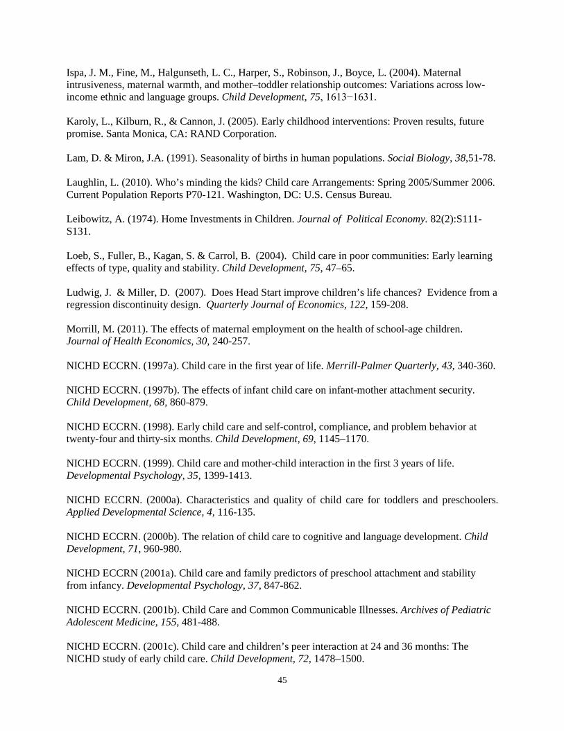
45

Ispa, J. M., Fine, M., Halgunseth, L. C., Harper, S., Robinson, J., Boyce, L. (2004). Maternal intrusiveness, maternal warmth, and mother–toddler relationship outcomes: Variations across low-income ethnic and language groups. Child Development, 75, 1613−1631. Karoly, L., Kilburn, R., & Cannon, J. (2005). Early childhood interventions: Proven results, future promise. Santa Monica, CA: RAND Corporation. Lam, D. & Miron, J.A. (1991). Seasonality of births in human populations. Social Biology, 38,51-78. Laughlin, L. (2010). Who’s minding the kids? Child care Arrangements: Spring 2005/Summer 2006. Current Population Reports P70-121. Washington, DC: U.S. Census Bureau. Leibowitz, A. (1974). Home Investments in Children. Journal of Political Economy. 82(2):S111-S131. Loeb, S., Fuller, B., Kagan, S. & Carrol, B. (2004). Child care in poor communities: Early learning effects of type, quality and stability. Child Development, 75, 47–65. Ludwig, J. & Miller, D. (2007). Does Head Start improve children’s life chances? Evidence from a regression discontinuity design. Quarterly Journal of Economics, 122, 159-208. Morrill, M. (2011). The effects of maternal employment on the health of school-age children. Journal of Health Economics, 30, 240-257. NICHD ECCRN. (1997a). Child care in the first year of life. Merrill-Palmer Quarterly, 43, 340-360. NICHD ECCRN. (1997b). The effects of infant child care on infant-mother attachment security. Child Development, 68, 860-879. NICHD ECCRN. (1998). Early child care and self-control, compliance, and problem behavior at twenty-four and thirty-six months. Child Development, 69, 1145–1170. NICHD ECCRN. (1999). Child care and mother-child interaction in the first 3 years of life. Developmental Psychology, 35, 1399-1413. NICHD ECCRN. (2000a). Characteristics and quality of child care for toddlers and preschoolers. Applied Developmental Science, 4, 116-135. NICHD ECCRN. (2000b). The relation of child care to cognitive and language development. Child Development, 71, 960-980. NICHD ECCRN (2001a). Child care and family predictors of preschool attachment and stability from infancy. Developmental Psychology, 37, 847-862. NICHD ECCRN. (2001b). Child Care and Common Communicable Illnesses. Archives of Pediatric Adolescent Medicine, 155, 481-488. NICHD ECCRN. (2001c). Child care and children’s peer interaction at 24 and 36 months: The NICHD study of early child care. Child Development, 72, 1478–1500.

46

NICHD ECCRN. (2003a). Child Care and Common Communicable Illnesses in Children Aged 37 to 54 Months. Archives of Pediatric Adolescent Medicine, 157, 196-200. NICHD ECCRN. (2003b). Does amount of time spent in child care predict socioemotional adjustment during the transition to kindergarten? Child Development, 74, 976–1005. NICHD ECCRN. (2004). Type of child care and children’s development at 54-months. Early Childhood Research Quarterly, 19, 203-230. NICHD ECCRN & Duncan, G. (2003). Modeling the impacts of child care quality on children’s preschool cognitive development. Child Development, 74, 1454-1475. Pianta, R., W. Steven Barnett, Margaret Burchinal, & Kathy R. Thornburg. (2009). The Effects of preschool education: What we know, how public policy is or is not aligned with the evidence base, and what we need to know. Psychological Science in the Public Interest, 10, 49–88. Peisner-Feinberg, E., Burchinal, M., Clifford, R., Culkin, M., Howes, C., Kagan, S., & Yazejian, N. (2001). The relation of preschool child-care quality to children’s cognitive and social development trajectories through second grade. Child Development, 72, 1534-1553. Raver, C. (2002). Emotions matter: Making the case for the role of young children’s emotional development for early school readiness. Social Policy Report of the Society for Research in Child Development, 16, 1–20. Ruhm, C. (2004). Parental employment and child cognitive development. Journal of Human Resources, 39, 155-192. U.S. Department of Health and Human Services, Administration for Children and Families. (2005). Head start impact study: First year findings. Washington, DC: U.S. Department of Health and Human Services. U.S. Department of Health and Human Services, Administration for Children and Families. (2010). Head start impact study: Final report. Washington, DC: U.S. Department of Health and Human Services. Todd, P. & Wolpin, K. (2003). On the specification and estimation of the production function for cognitive achievement. The Economic Journal, 113, F3-F33. Todd, P. & Wolpin, K. (2007). The production of cognitive achievement in children: Home, school, and racial test score gaps. Journal of Human Capital, 1, 91-136. Wong, V.C., Cook, T.D., Barnett, W.S., & Jung, K. (2008). An effectiveness-based evaluation of five state pre-kindergarten programs. Journal of Policy Analysis and Management, 27, 122–154.

48

0.1

0.2

0.3

0.4

0.5

0.6

0.7

0.8

0.9

1.0

Perc

ent

Oct-

01De

c-01

Feb-

02Ap

r-02

Jun-

02Au

g-02

Oct-

02De

c-02

Feb-

03Ap

r-03

Jun-

03Au

g-03

Oct-

03De

c-03

Month of Interview

9-month Wave 24-month Wave

Child is Male

0.1

0.2

0.3

0.4

0.5

0.6

0.7

0.8

0.9

1.0

Perc

ent

Oct-

01De

c-01

Feb-

02Ap

r-02

Jun-

02Au

g-02

Oct-

02De

c-02

Feb-

03Ap

r-03

Jun-

03Au

g-03

Oct-

03De

c-03

Month of Interview

9-month Wave 24-month Wave

Child is White

0.1

0.2

0.3

0.4

0.5

0.6

0.7

0.8

0.9

1.0

Perc

ent

Oct-

01De

c-01

Feb-

02Ap

r-02

Jun-

02Au

g-02

Oct-

02De

c-02

Feb-

03Ap

r-03

Jun-

03Au

g-03

Oct-

03De

c-03

Month of Interview

9-month Wave 24-month Wave

Low Birth Weight

0.1

0.20.3

0.40.5

0.6

0.70.8

0.9

1.0

Perc

ent

Oct-

01De

c-01

Feb-

02Ap

r-02

Jun-

02Au

g-02

Oct-

02De

c-02

Feb-

03Ap

r-03

Jun-

03Au

g-03

Oct-

03De

c-03

Month of Interview

9-month Wave 24-month Wave

Premature Birth

Figure 2: Child Characteristics by Month of ECLS-B Assessment

49

0.1

0.2

0.3

0.4

0.5

0.6

0.7

0.8

0.9

1.0

Perc

ent

Oct-

01De

c-01

Feb-

02Ap

r-02

Jun-

02Au

g-02

Oct-

02De

c-02

Feb-

03Ap

r-03

Jun-

03Au

g-03

Oct-

03De

c-03

Month of Interview

9-month Wave 24-month Wave

Mother is Single, Never Married

0.1

0.2

0.3

0.4

0.5

0.6

0.7

0.8

0.9

1.0

Perc

ent

Oct-

01De

c-01

Feb-

02Ap

r-02

Jun-

02Au

g-02

Oct-

02De

c-02

Feb-

03Ap

r-03

Jun-

03Au

g-03

Oct-

03De

c-03

Month of Interview

9-month Wave 24-month Wave

Mother is a High School Drop-Out

0.1

0.2

0.3

0.4

0.5

0.6

0.7

0.8

0.9

1.0

Perc

ent

Oct-

01De

c-01

Feb-

02Ap

r-02

Jun-

02Au

g-02

Oct-

02De

c-02

Feb-

03Ap

r-03

Jun-

03Au

g-03

Oct-

03De

c-03

Month of Interview

9-month Wave 24-month Wave

Mother is in 'Excellent'/'Very Good' Health

0.1

0.2

0.3

0.4

0.5

0.6

0.7

0.8

0.9

1.0

Per

cent

Oct-

01De

c-01

Feb-

02Ap

r-02

Jun-

02Au

g-02

Oct-

02De

c-02

Feb-

03Ap

r-03

Jun-

03Au

g-03

Oct-

03De

c-03

Month of Interview

9-month Wave 24-month Wave

Mother is Employed

0.1

0.2

0.3

0.4

0.5

0.6

0.7

0.8

0.9

1.0

Per

cent

Oct-

01De

c-01

Feb-

02Ap

r-02

Jun-

02Au

g-02

Oct-

02De

c-02

Feb-

03Ap

r-03

Jun-

03Au

g-03

Oct-

03De

c-03

Month of Interview

9-month Wave 24-month Wave

Household is in the Bottom SES Quintile

0.1

0.2

0.3

0.4

0.5

0.6

0.7

0.8

0.9

1.0

Per

cent

Oct

-01

Dec-

01Fe

b-02

Apr-0

2Ju

n-02

Aug-

02O

ct-0

2De

c-02

Feb-

03Ap

r-03

Jun-

03Au

g-03

Oct

-03

Dec-

03

Month of Interview

9-month Wave 24-month Wave

Household is in the Top SES Quintile

Figure 3: Family Characteristics by Month of ECLS-B Assessment

50

Table 1: Summary Statistics Variable

Full Sample

Non-Parental Child Care

Parental Child Care

Outcome Bailey Short Form mental test score (9-months) 74.84

(10.08) 75.34

(10.05) 74.34

(10.07) Bailey Short Form mental test score (24-months) 125.53

(10.99) 126.40 (11.05)

124.67 (10.87)

Child Characteristics Male (%) 0.511

(0.500) 0.512

(0.500) 0.510

(0.500) Age (months)

17.14 (7.14)

17.15 (7.13)

17.12 (7.14)

White (%)

0.421 (0.494)

0.409 (0.492)

0.432 (0.495)

Low birth weight (%)

0.263 (0.440)

0.262 (0.440)

0.264 (0.441)

Premature birth (%)

0.115 (0.319)

0.114 (0.318)

0.116 (0.320)

Weight (kilograms)

10.85 (2.44)

10.92 (2.42)

10.77 (2.45)

Family Characteristics Mother’s age (years)

29.17 (6.67)

29.11 (6.71)

29.23 (6.63)

Mother is single, never married (%)

0.266 (0.442)

0.294 (0.456)

0.238 (0.426)

Mother is married (%)

0.668 (0.471)

0.626 (0.484)

0.708 (0.455)

Mother is a high school drop-out (%)

0.179 (0.383)

0.129 (0.336)

0.227 (0.419)

Mother has a BA+ (%)

0.269 (0.443)

0.300 (0.458)

0.238 (0.426)

Mother is employed (%)

0.523 (0.500)

0.818 (0.386)

0.233 (0.423)

Household income ($/1,000)

51.558 (45.402)

57.317 (48.518)

45.871 (41.321)

Focal child is an only-child (%)

0.335 (0.472)

0.382 (0.486)

0.287 (0.453)

Urban residence (%)

0.847 (0.361)

0.842 (0.364)

0.851 (0.357)

Source: Author’s analysis of the 9- and 24-month waves of the ECLS-B. Notes: Standard deviations are displayed in parentheses. The means come from the pooled 9- and 24-month sample.

51

Table 2: Child Care Participation Profile at 9- and 24-Months Variable

Pooled Periods

9-Month Survey

24-Month Survey

Panel A: Primary Measure Non-parental child care (%)

0.497 (0.500)

0.499 (0.500)

0.494 (0.500)

Average weekly hours (no.)

32.68 (17.26)

32.15 (18.26)

33.28 (16.06)

Panel B: Alternative Measure Informal child care (%)

0.270 (0.444)

0.301 (0.462)

0.227 (0.419)

Average weekly hours (no.)

28.49 (16.72)

27.41 (16.96)

30.12 (16.23)

Formal child care (%)

0.224 (0.417)

0.186 (0.389)

0.265 (0.441)

Average weekly hours (no.)

32.20 (13.61)

32.12 (13.91)

32.26 (13.39)

Panel C: Alternative Measure Cumulative Child Care (no. months) 6.76

(8.09) 3.66

(3.96) 10.92

(10.09) Source: Author’s analysis of the 9- and 24-month waves of the ECLS-B. Notes: Standard deviations are displayed in parentheses. Informal care includes relative care in any home and non-relative care in the child’s home. Formal care includes non-relative care in another’s home and center-based care. The figures for average weekly hours in Panel A represent the sum of hours in non-parental child care over all arrangements. The analogous figures in Panel B represent the number of hours in informal or formal care for the arrangement in which the child spent the greatest number of hours. All hours of care calculations are based on the sub-set of children using non-parental child care.

52

Table 3: ECLS-B Assessment Schedule Month and Year of Assessment

Number of Assessments

Wave 1: 9-Month Survey Oct-01 97 Nov-01 934 Dec-01 685 Jan-02 954 Feb-02 911 Mar-02 551 Apr-02 900 May-02 826 Jun-02 816 July-02 865 Aug-02 935 Sep-02 813 Oct-02 538 Nov-02 289 Dec-02

66

Wave 2: 24-Month Survey Jan-03 237 Feb-03 994 Mar-03 1,047 Apr-03 925 May-03 837 Jun-03 740 Jul-03 822 Aug-03 831 Sep-03 795 Oct-03 822 Nov-03 704 Dec-03 466 Apr-04 16 Source: Author’s analysis of the 9- and 24-month waves of the ECLS-B

53

Table 4: First-Stage Estimates of the Relationship between ECLS-B Assessment Timing and Current Non-Parental Child Care Utilization

Non-Parental Care Informal Care Formal Care Variable (1) (2) (3) (4) (5) Summer assessment -0.026***

(0.006) -0.027***

(0.006) -0.027***

(0.006) -0.024***

(0.007) -0.023***

(0.007) F-statistic (p-value) 17.53

(0.000) 19.63

(0.000) 18.74

(0.000) 12.57

(0.000) 11.62

(0.000) Child characteristics Y Y Y Y Y Family characteristics Y Y Y Y Y Family characteristics × wave Y Y Y Y Y State fixed effects with wave interactions N Y Y Y Y Quarter-of-birth N N Y N N Number of observations 19,416 19,416 19,416 14,976 14,079 Source: Author’s analysis of the 9- and 24-month waves of the ECLS-B. Notes: Standard errors are displayed in parentheses and are adjusted for within-child clustering. The summer assessment variable is a binary indicator for whether a given child was assessed (and parents were interviewed) in the summer (i.e., June, July, August, or September) during the 9- or 24-month survey. The dependent variable in columns (1) through (3) is a binary indicator for participation in any non-parental child care arrangement. The dependent variable in column (4) is a binary indicator for participation in an informal arrangement (and equals zero for participation in parent care). The dependent variable in column (5) is a binary indicator for participation in a formal arrangement (and equals zero for participation in parent care). The child characteristics include gender, age (up to a quartic polynomial), race and ethnicity (four dummy variables), low birth weight (one dummy variable), premature birth (one dummy variable), and weight (in kilograms). The family controls include mother’s age (up to a squared polynomial), marital status (four dummy variables), mother’s education (three dummy variables), the presence of other siblings in the household (three dummy variables), mother’s employment status (three dummy variables), total household income (12 dummy variables), and urban residence (one dummy variable). All models include a binary indicator for wave. ***, **, * indicate statistical significance at the 0.01, 0.05, and 0.10 levels, respectively.

54

Table 5: Child Characteristics by Month of ECLS-B Assessment Month of Assessment

Male (1)

White (2)

LBW (3)

Premature (4)

Weight (5)

Panel A: No Controls June

-0.007 (0.014)

0.000 (0.014)

0.014 (0.012)

0.012 (0.009)

-0.036 (0.048)

July

-0.000 (0.013)

-0.019 (0.013)

0.017 (0.012)

0.009 (0.009)

-0.035 (0.049)

August

0.002 (0.013)

0.007 (0.013)

0.026** (0.012)

0.017* (0.009)

-0.050 (0.048)

September

-0.011 (0.014)

-0.011 (0.013)

0.020 (0.012)

0.008 (0.009)

0.036 (0.051)

F-statistic (p-value)

0.24 (0.918)

0.80 (0.527)

1.88 (0.111)

1.26 (0.285)

0.67 (0.615)

Panel B: Includes Controls June

-0.003 (0.014)

-0.002 (0.011)

-0.002 (0.010)

0.006 (0.007)

-0.053 (0.044)

July

0.002 (0.013)

-0.017 (0.011)

0.006 (0.010)

0.002 (0.007)

-0.065 (0.044)

August

0.004 (0.013)

-0.003 (0.011)

0.012 (0.009)

0.011 (0.007)

-0.025 (0.043)

September

-0.012 (0.014)

-0.007 (0.012)

0.012 (0.010)

-0.002 (0.007)

-0.004 (0.046)

F-statistic (p-value)

0.28 (0.894)

0.60 (0.662)

0.84 (0.502)

0.72 (0.581)

0.84 (0.501)

Number of observations 19,416 19,379 19,339 19,032 18,590 Source: Author’s analysis of the 9- and 24-month waves of the ECLS-B. Notes: Standard errors are displayed in parentheses and are adjusted for within-child clustering. LBW is low birth weight. See Table 4 for a list of the controls included in the models in Panel B. Panel B also includes state fixed effects with wave interactions. All models include a binary indicator for wave. ***, **, * indicate statistical significance at the 0.01, 0.05, and 0.10 levels, respectively.

55

Table 6: Family Characteristics by Month of ECLS-B Assessment Month of Assessment

Never Married

(1)

High School Drop-Out

(2)

Excell/VG Health

(3)

Bottom SES Quintile

(4)

Top SES Quintile

(5) Panel A: No Controls June

0.008 (0.012)

-0.023** (0.010)

-0.007 (0.013)

-0.028*** (0.010)

-0.002 (0.011)

July

0.008 (0.012)

0.001 (0.010)

0.006 (0.012)

0.009 (0.011)

-0.009 (0.011)

August

-0.001 (0.011)

-0.014 (0.010)

0.007 (0.012)

-0.001 (0.010)

0.012 (0.011)

September

0.017 (0.012)

-0.011 (0.010)

-0.010 (0.013)

0.003 (0.011)

0.003 (0.011)

F-statistic (p-value)

0.61 (0.652)

1.80 (0.126)

0.46 (0.765)

2.25 (0.061)

0.65 (0.628)

Panel B: Includes Controls June

0.005 (0.009)

-0.017* (0.009)

-0.007 (0.012)

-0.022** (0.009)

0.003 (0.010)

July

-0.002 (0.009)

-0.003 (0.009)

0.008 (0.012)

-0.001 (0.009)

-0.000 (0.009)

August

-0.001 (0.009)

-0.011 (0.009)

0.010 (0.012)

-0.003 (0.009)

0.018* (0.009)

September

0.005 (0.010)

-0.015 (0.009)

-0.011 (0.012)

-0.007 (0.009)

0.010 (0.010)

F-statistic (p-value)

0.17 (0.956)

1.47 (0.209)

0.66 (0.622)

1.50 (0.199)

1.12 (0.346)

Number of observations 19,215 19,353 19,414 19,416 19,416 Source: Author’s analysis of the 9- and 24-month waves of the ECLS-B. Notes: Standard errors are displayed in parentheses and are adjusted for within-child clustering. The outcomes in columns (1) through (3) relate to the focal child’s mother. The outcome in column (3) is a binary indicator for whether a given mother self-reports being in “excellent” or “very good” health. See Table 4 for a list of the controls included in the models in Panel B. Panel B also includes state fixed effects with wave interactions. All models include a binary indicator for wave. ***, **, * indicate statistical significance at the 0.01, 0.05, and 0.10 levels, respectively.

56

Table 7: Comparison of Non-Parental Child Care Environments across the Summer and Non-Summer Months, 24-Month Wave

Coefficient on Summer Assessment

Dependent Variable N Mean (1) (2) Panel A: Global Child Care Quality ITERS for center-based settings (range: 1-7)

596 4.163 0.003 (0.086)

-0.110 (0.086)

FDCRS for home-based settings (range: 1-7)

776 3.403 0.004 (0.079)

-0.011 (0.070)

Arnett Scale of Caregiver Behavior

1,359 60.85 -0.086 (0.613)

-0.237 (0.591)

Panel B: Characteristics of the Child Care Center Director B.A. degree or more (%)

568 0.528 -0.025 (0.044)

0.006 (0.045)

Child Development Associate credential (%)

561 0.301 -0.031 (0.040)

-0.043 (0.044)

Degree in early childhood education (%)

568 0.489 -0.010 (0.044)

-0.015 (0.045)

Experience in child care/education (years)

570 14.79 -2.104*** (0.708)

-1.570* (0.818)

Panel C: Characteristics of the Caregiver Female (%)

3,066 0.967 -0.001 (0.007)

0.002 (0.007)

Born in the U.S. (%)

3,058 0.810 0.004 (0.015)

-0.005 (0.013)

Black (%)

3,032 0.211 0.030* (0.016)

-0.010 (0.011)

High school degree or more (%)

3,057 0.826 -0.010 (0.015)

-0.010 (0.015)

Child Development Associate credential (%)

2,517 0.167 0.045*** (0.016)

0.029* (0.016)

Experience in child care field (years)

3,052 9.742 -0.261 (0.361)

-0.256 (0.367)

Reported health is excellent/very good (%)

3,058 0.712 0.004 (0.018)

0.008 (0.018)

Smokes cigarettes (%)

3,059 0.133 -0.004 (0.013)

-0.013 (0.013)

Time difference: child/provider assessment Y Y Child characteristics N Y Family characteristics N Y State fixed effects N Y Source: Author’s analysis of the 24-month wave of the ECLS-B. Notes: Standard errors are displayed in parentheses and are robust to arbitrary forms of heteroskedasticity. See Table 4 for a list of the controls included in the models. Presented in columns (1) and (2) is the coefficient on the summer assessment instrumental variable. Column (1) controls only for whether the relevant child care provider information was collected within one month of the child assessment. Column (2) adds the full set of controls. ***, **, * indicate statistical significance at the 0.01, 0.05, and 0.10 levels, respectively.

57

Table 8: The Relationship between Assessment and Birth Timing in the ECLS-B Quarter-of-Birth (2001, %) Month-of-Assessment QOB-1 QOB-2 QOB-3 QOB-4 Panel A: 9-Month Survey (2002) June

0.048 (0.213)

0.214 (0.411)

0.708 (0.455)

0.029 (0.169)

July

0.042 (0.200)

0.123 (0.328)

0.468 (0.499)

0.368 (0.482)

August

0.026 (0.158)

0.062 (0.241)

0.244 (0.430)

0.669 (0.471)

September

0.028 (0.166)

0.058 (0.234)

0.191 (0.393)

0.723 (0.448)

Panel B: 24-Month Survey (2003) June

0.107 (0.309)

0.815 (0.387)

0.078 (0.269)

0.000 (0.000)

July

0.024 (0.154)

0.313 (0.464)

0.663 (0.473)

0.000 (0.000)

August

0.018 (0.133)

0.108 (0.311)

0.865 (0.342)

0.008 (0.091)

September

0.016 (0.127)

0.058 (0.234)

0.689 (0.463)

0.237 (0.425)

Source: Author’s analysis of the 9- and 24-month waves of the ECLS-B. Notes: Standard deviations are displayed in parentheses. Each cell depicts the fraction of children born in each calendar quarter (quarter-of-birth) by the summer month in which children are assessed (month-of-interview) during the 9- and 24-month surveys. Each row sums to one (100 percent).

58

Table 9: OLS and Fixed Effects Estimates of the Impact of Current Non-Parental Child Care Utilization Variable

OLS (1)

OLS (2)

OLS (3)

OLS (4)

Child FE (5)

Child FE (6)

Non-parental child care

0.014*** (0.002)

0.010*** (0.001)

0.003* (0.002)

0.003* (0.002)

0.008*** (0.003)

0.004* (0.002)

Child characteristics N Y Y Y N Y Family characteristics N N Y Y N Y Family characteristics × wave N N Y Y N Y State fixed effects with wave interactions N N N Y N N Source: Author’s analysis of the 9- and 24-month waves of the ECLS-B. Notes: Standard errors are displayed in parentheses and are adjusted for within-child clustering. The outcome in all models is the natural log of the Bailey Short Form-Research Edition mental test score. The omitted category in Panel B is parental child care. Informal care includes relative care in any home and non-relative care in the child’s home. Formal care includes non-relative care in another’s home and center-based care. See Table 4 for a list of the controls included in the models. All models include a binary indicator for wave. All analyses are based on 10,201 children, providing 19,071 child-wave combinations. ***, **, * indicate statistical significance at the 0.01, 0.05, and 0.10 levels, respectively.

59

Table 10: Instrumental Variables Estimates of the Impact of Current Non-Parental Child Care Utilization Variable

First Stage

(1)

Reduced Form

(2)

IV 2SLS

(3)

IV 2SLS

(4)

IV FE-1 (5)

IV FE-2 (6)

Non-parental child care / Summer assessment

-0.026*** (0.006)

0.003** (0.001)

-0.094** (0.039)

-0.085** (0.039)

-0.105 (0.146)

-0.092* (0.054)

Child characteristics Y Y Y Y Y Y Family characteristics Y Y Y Y Y Y Family characteristics × wave Y Y Y Y Y Y State fixed effects with wave interactions Y Y Y Y N N Quarter-of-birth N N N Y N N Source: Author’s analysis of the 9- and 24-month waves of the ECLS-B. Notes: Standard errors are displayed in parentheses and are adjusted for within-child clustering. The outcome column (1) is the binary indicator of non-parental child care utilization. The outcome in columns (2) through (6) is the log of the Bailey Short Form Research-Edition mental test score. The instrument in columns (3) through (5) is the binary indicator for a summer assessment. The instruments in column (6) include a set of binary indicators for each summer month (i.e., June through September) in each ECLS-B survey wave (i.e., 9- and 24-month), for a total of eight instruments. See Table 4 for a list of the controls included in the models. All models include a binary indicator for wave. All analyses are based on 10,201 children, providing 19,071 child-wave combinations. ***, **, * indicate statistical significance at the 0.01, 0.05, and 0.10 levels, respectively.

60

Table 11: OLS, Fixed Effects, and Instrumental Variables Estimates of the Impact of Cumulative Non-Parental Child Care Utilization

Variable

First Stage

(1)

First Stage

(2)

OLS Full (3)

Child FE (4)

IV 2SLS (5)

IV 2SLS (6)

Summer assessment / Cumulative child care

-0.385*** (0.096)

-0.368*** (0.099)

0.0004*** (0.0001)

0.001** (0.0002)

-0.008** (0.003)

-0.007** (0.003)

F-statistic (p-value) 16.23 13.73 N/A N/A N/A N/A Child characteristics Y Y Y Y Y Y Family characteristics Y Y Y Y Y Y State fixed effects with wave interactions Y Y Y N Y Y Quarter-of-birth N Y N N N Y Source: Author’s analysis of the 9- and 24-month waves of the ECLS-B. Notes: Standard errors are displayed in parentheses and are adjusted for within-child clustering. The outcome in columns (1) and (2) is the measure of cumulative non-parental child care utilization (i.e., number of months in any non-parental arrangement). The outcome in columns (3) through (6) is the log of the Bailey Short Form Research-Edition mental test score. The instrument in columns (5) through (6) is the binary indicator for a summer assessment. See Table 4 for a list of the controls included in the models. All models include a binary indicator for wave and a control for the age at which the focal child experienced the first non-parental child care arrangement. ***, **, * indicate statistical significance at the 0.01, 0.05, and 0.10 levels, respectively.

61

Table 12: Robustness Checks Specification

Coefficient on Current Child Care

(Standard Error) (1)

Coefficient on Cumulative Child Care

(Standard Error) (2)

(1) Control for parent reports of child’s health

-0.085** (0.039)

-0.007** (0.003)

(2) Control for child asthma and ear infections

-0.095** (0.041)

-0.008** (0.003)

(3) Control for child injuries

-0.091** (0.040)

-0.008** (0.003)

(4) Control for self-reported maternal health

-0.087** (0.040)

-0.008** (0.003)

(5) Control for maternal occupation

-0.094** (0.037)

-0.007** (0.003)

(6) Control for January births

-0.091** (0.040)

-0.008** (0.003)

(7) Control for state conditions at child’s birth

-0.103* (0.062)

-0.007 (0.005)

(8) Omit children living in the South

-0.098** (0.042)

-0.008** (0.004)

(9) Classify June as a non-summer month

-0.065* (0.038)

-0.004 (0.003)

(10) Omit June from the analysis

-0.071* (0.038)

-0.005* (0.003)

(11) Classify Sept. as a non-summer month

-0.102** (0.040)

-0.010*** (0.003)

(12) Omit Sept. from the analysis

-0.114*** (0.039)

-0.010*** (0.004)

(13) Omit control for maternal employment

-0.132** (0.052)

-0.009** (0.004)

(14) Omit control for household income

-0.095** (0.039)

-0.009*** (0.003)

Source: Author’s analysis of the 9- and 24-month waves of the ECLS-B. Notes: Standard errors are displayed in parentheses and are adjusted for within-child clustering. The outcome in all models is the log of the Bailey Short Form Research-Edition mental test score. The instrument in all models is the binary indicator for a summer assessment. See Table 4 for a list of the controls included in the models. All models include a binary indicator for wave, and those in column (2) include a control for the age at which the focal child experienced the first non-parental child care arrangement. ***, **, * indicate statistical significance at the 0.01, 0.05, and 0.10 levels, respectively.

62

Table 13: Alternative Instrument Sets and IV Estimator Variable

2SLS (1A)

LIML (1B)

2SLS (2A)

LIML (2B)

2SLS (3A)

LIML (3B)

Non-parental child care

-0.099** (0.039)

-0.112** (0.045)

-0.087** (0.039)

-0.104** (0.046)

-0.097** (0.039)

-0.145** (0.061)

Instrument set (number)

Dummies for summer assessment at 9- and

24-months (2)

Dummies for June, July, Aug, Sept assessment (4)

Dummies for June, July, Aug, Sept assessment at

9- and 24-months (8)

Test of overidentifying restrictions: p-value 0.569 0.543 0.211 Child characteristics Y Y Y Y Y Y Family characteristics Y Y Y Y Y Y Family characteristics × wave Y Y Y Y Y Y State fixed effects with wave interactions Y Y Y Y Y Y Source: Author’s analysis of the 9- and 24-month waves of the ECLS-B. Notes: Standard errors are displayed in parentheses and are adjusted for within-child clustering. The outcome in all models the log of the Bailey Short Form Research-Edition mental test score. The instruments in columns (1A) and (1B) are separate binary indicators for a summer assessment in the 9- and 12-month waves. The instruments in columns (2A) and (2B) are separate binary indicators for each summer assessment month (i.e., June through September) irrespective of wave. The instruments in columns (3A) and (3B) are separate binary indicators for each summer assessment month in both the 9- and 12-month waves. The test of overidentifying restrictions is the Wooldridge Score test. See Table 4 for a list of the controls included in the models. All models include a binary indicator for wave. All analyses are based on 10,201 children, providing 19,071 child-wave combinations. ***, **, * indicate statistical significance at the 0.01, 0.05, and 0.10 levels, respectively.

63

Table 14: OLS and Instrumental Variables Estimates of the Impact of Current Informal and Formal Child Care Utilization

Variable

OLS Full (1)

Child FE Full (2)

IV 2SLS (3)

Informal child care (vs. parental care)

0.002 (0.002)

0.006** (0.003)

-0.052 (0.050)

Formal child care (vs. parental care)

0.004** (0.002)

0.003 (0.003)

-0.131*** (0.043)

Child characteristics Y Y Y Family characteristics Y Y Y Family characteristics × wave Y Y Y State fixed effects with wave interactions Y N Y Quarter-of-birth N N N Source: Author’s analysis of the 9- and 24-month waves of the ECLS-B. Notes: Standard errors are displayed in parentheses and are adjusted for within-child clustering. In columns (1) and (2), a single regression of test scores is estimated on separate binary indicators of informal and formal child care utilization. In column (3), each cell represents a different regression of test scores on the corresponding child care arrangement. See Table 4 for a list of the controls included in the models. All models include a binary indicator for wave. ***, **, * indicate statistical significance at the 0.01, 0.05, and 0.10 levels, respectively.

64

Table 15: Heterogeneous Effects of Current Non-Parental Child Care Utilization Demographic Sub-Group

OLS (1)

Child FE (2)

IV 2SLS (3)

Focal child is male

0.004 (0.002)

0.002 (0.003)

-0.064 (0.074)

Focal child is female

0.002 (0.002)

0.006* (0.003)

-0.090 (0.067)

Focal child is white

0.002 (0.002)

0.005 (0.004)

-0.202* (0.106)

Focal child is non-white

0.003 (0.002)

0.003 (0.003)

-0.018 (0.038)

Mother is married

0.003 (0.002)

0.003 (0.003)

-0.171** (0.084)

Mother is unmarried

0.002 (0.003)

0.007* (0.004)

-0.034 (0.077)

Mother has a high school degree or less

0.001 (0.002)

0.008** (0.003)

-0.180 (0.122)

Mother has more than a high school degree

0.005** (0.002)

0.002 (0.003)

-0.072 (0.059)

Mother is employed

-0.000 (0.002)

0.004 (0.004)

-0.139*** (0.038)

Moth is not employed

0.006** (0.002)

0.006 (0.004)

-0.057 (0.063)

Household SES is in bottom two quintiles

0.003 (0.002)

0.008** (0.004)

-0.024 (0.045)

Household SES is in top three quintiles

0.002 (0.002)

0.003 (0.003)

-0.092** (0.038)

Source: Author’s analysis of the 9- and 24-month waves of the ECLS-B. Notes: Standard errors are displayed in parentheses and are adjusted for within-child clustering. The outcome in all models is the log of the Bailey Short Form Research-Edition mental test score. The instrument in all models the binary indicator for a summer assessment. See Table 4 for a list of the controls included in the models. All models include a binary indicator for wave. ***, **, * indicate statistical significance at the 0.01, 0.05, and 0.10 levels, respectively.

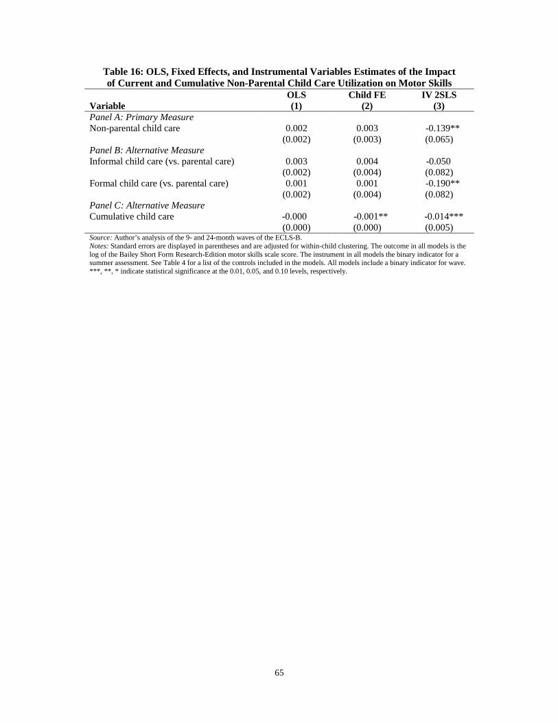
65

Table 16: OLS, Fixed Effects, and Instrumental Variables Estimates of the Impact of Current and Cumulative Non-Parental Child Care Utilization on Motor Skills

Variable

OLS (1)

Child FE (2)

IV 2SLS (3)

Panel A: Primary Measure Non-parental child care

0.002 (0.002)

0.003 (0.003)

-0.139** (0.065)

Panel B: Alternative Measure Informal child care (vs. parental care)

0.003 (0.002)

0.004 (0.004)

-0.050 (0.082)

Formal child care (vs. parental care)

0.001 (0.002)

0.001 (0.004)

-0.190** (0.082)

Panel C: Alternative Measure Cumulative child care

-0.000 (0.000)

-0.001** (0.000)

-0.014*** (0.005)

Source: Author’s analysis of the 9- and 24-month waves of the ECLS-B. Notes: Standard errors are displayed in parentheses and are adjusted for within-child clustering. The outcome in all models is the log of the Bailey Short Form Research-Edition motor skills scale score. The instrument in all models the binary indicator for a summer assessment. See Table 4 for a list of the controls included in the models. All models include a binary indicator for wave. ***, **, * indicate statistical significance at the 0.01, 0.05, and 0.10 levels, respectively.

66

Appendix Table 1: The Relationship between ECLS-B Assessment Timing and Non-Parental Child Care Utilization by Demographic Sub-Group

Demographic Sub-Group

Coefficient on Summer Assessment

(Standard Error) Focal child is male

-0.024*** (0.009)

Focal child is female

-0.031*** (0.009)

Focal child is white

-0.028*** (0.009)

Focal child is non-white

-0.030*** (0.008)

Mother is married

-0.027*** (0.008)

Mother is unmarried

-0.028** (0.011)

Mother has a high school degree or less

-0.021** (0.009)

Mother has more than a high school degree

-0.033*** (0.009)

Mother is employed

-0.023** (0.009)

Mother is not employed

-0.032*** (0.009)

Household SES is in bottom two quintiles

-0.020** (0.010)

Household SES is in top three quintiles

-0.032*** (0.008)

Focal child is an only-child

-0.015 (0.010)

Focal child has one or more siblings

-0.034*** (0.008)

Household has one adult ages 18+

-0.017 (0.018)

Household has two adults ages 18+

-0.025*** (0.007)

Household has three or more adults ages 18+

-0.039*** (0.015)

Source: Author’s analysis of the 9- and 24-month waves of the ECLS-B. Notes: Standard errors are displayed in parentheses and are adjusted for within-child clustering. The dependent is a binary indicator for participation in any non-parental child care arrangement. The summer assessment variable is a binary indicator for whether a given family was interviewed and the child was assessed in the summer (i.e., June, July, August, or September) during the 9- or 24-month wave. See Table 4 for a list of the controls included in the models. All models include a binary indicator for wave. ***, **, * indicate statistical significance at the 0.01, 0.05, and 0.10 levels, respectively.

67

Appendix Table 2: Summer Maternal Work Activity Work vs.

No Work Part- vs. Full-Time Work

Full-Time vs. No Work

Part-Time vs. No Work

Looking vs. No Work

Variable (1) (2) (3) (4) (5) Summer assessment 0.000

(0.008)

-0.015 (0.010)

0.001 (0.008)

-0.008 (0.009)

-0.011 (0.008)

Child characteristics Y Y Y Y Y Family characteristics Y Y Y Y Y Family characteristics × wave Y Y Y Y Y State fixed effects with wave interactions Y Y Y Y Y Number of observations 19,312 10,098 14,320 11,278 9,214 Source: Author’s analysis of the 9- and 24-month waves of the ECLS-B. Notes: Standard errors are displayed in parentheses and are adjusted for within-child clustering. The summer assessment variable is a binary indicator for whether a given family was interviewed and the child was assessed in the summer (i.e., June, July, August, or September) during the 9- or 24-month wave. The dependent variable in column (1) equals unity for employed mothers and zero for mothers not in the labor force. The dependent variable in column (2) equals unity for full-time working mothers (employed 35+ hours per week) and zero for part-time working mothers. The dependent variables in columns (3) and (4) equal unity for full-time and part-time working mothers, respectively, and zero for mothers not in the labor force. The dependent variable in column (5) equals unity for mothers looking for work and zero for mothers not in the labor force. See Table 4 for a list of the controls included in the models (the models presented here exclude the maternal employment controls). All models include a binary indicator for wave. ***, **, * indicate statistical significance at the 0.01, 0.05, and 0.10 levels, respectively.

68

Appendix Table 3: Summer Non-Parental Child Care Utilization by Maternal Employment Status and Place of Employment

Variable

Regression Results

(1)

Child Care Utilization Rate

(2)

Implied Change in Utilization

(3) Panel A: By Employment Status Summer assessment × Works full-time

-0.023** (0.010)

0.838 -2.7%

× Works part-time

-0.023 (0.017)

0.659 -3.5%

× Looking for work

-0.061** (0.025)

0.339 -18.0%

× Not in labor force

-0.027*** (0.009)

0.162 -16.7%

Panel B: By Place of Employment Summer assessment × Works outside home

-0.010 (0.010)

0.801 -1.2%

× Works from home

-0.062*** (0.022)

0.725 -8.5%

× Self-employed

-0.021 (0.056)

0.484 -4.2%

× Unemployed

-0.035*** (0.009)

0.192 -18.1%

Child characteristics Y Family characteristics Y Family characteristics × wave Y State fixed effects with wave interactions Y Number of observations 19,312/19,410 Source: Author’s analysis of the 9- and 24-month waves of the ECLS-B. Notes: Standard errors are displayed in parentheses and are adjusted for within-child clustering. The summer interview variable is a binary indicator for whether a given family was interviewed and the child was assessed in the summer (i.e., June, July, August, or September) during the 9- or 24-month wave. The dependent variable in all models is a binary indicator for participation in any non-parental child care arrangement. See Table 4 for a list of the controls included in the models. All models include a binary indicator for wave. The model in Panel B replaces the controls for maternal employment status with separate dummy variables indicating the place of employment. ***, **, * indicate statistical significance at the 0.01, 0.05, and 0.10 levels, respectively.

Appendix Table 4: Summer Activities with the Focal Child by Maternal Employment Status and Place of Employment Variable

Read Stories Sing Songs

(1)

Run Errands

(2)

Walk/Play Yard/Park

(3)

Visit Zoo (4)

Visit Museum

(5)

Breakfast Together

(6)

Dinner Together

(7) Panel A: By Employment Status Summer assessment × Works full-time

0.017* (0.010)

0.043*** (0.013)

0.184*** (0.013)

0.114*** (0.017)

0.036*** (0.013)

0.027*** (0.009)

0.013* (0.007)

× Works part-time

0.022 (0.014)

0.039** (0.017)

0.228*** (0.017)

0.170*** (0.024)

0.020 (0.019)

0.014 (0.012)

0.024** (0.010)

× Looking for work

-0.022 (0.018)

0.060** (0.026)

0.152*** (0.027)

0.100*** (0.038)

0.026 (0.027)

0.016 (0.018)

0.032** (0.013)

× Not in labor force

-0.003 (0.009)

0.030** (0.012)

0.195*** (0.012)

0.109*** (0.016)

0.056*** (0.012)

0.012 (0.008)

0.001 (0.006)

Panel B: By Place of Employment Summer assessment × Works outside home

0.011 (0.009)

0.040*** (0.012)

0.190*** (0.012)

0.118*** (0.016)

0.033*** (0.011)

0.024*** (0.008)

0.012* (0.007)

× Works from home

0.047** (0.020)

0.047** (0.023)

0.235*** (0.023)

0.187*** (0.033)

0.031 (0.028)

0.025 (0.016)

0.032*** (0.012)

× Self-employed

-0.038 (0.044)

0.017 (0.055)

0.186*** (0.056)

0.079 (0.073)

-0.012 (0.052)

-0.056 (0.038)

0.034 (0.029)

× Unemployed

-0.004 (0.008)

0.036*** (0.011)

0.189*** (0.011)

0.106*** (0.015)

0.050*** (0.011)

0.013* (0.007)

0.007 (0.005)

Child characteristics Y Y Y Y Y Y Y Family characteristics Y Y Y Y Y Y Y Family characteristics × wave Y Y Y N N Y Y State fixed effects with wave interactions Y Y Y Y Y Y Y Outcome availability 9-/24-months 9-/24-months 9-/24-months 24-months 24-months 9-/24-months 9-/24-months Source: Author’s analysis of the 9- and 24-month waves of the ECLS-B. Notes: Standard errors are displayed in parentheses and are adjusted for within-child clustering. The summer interview variable is a binary indicator for whether a given family was interviewed and the child was assessed in the summer (i.e., June, July, August, or September) during the 9- or 24-month wave. All outcomes are defined as binary indicators of whether the respondent engaged in a given activity with the focal child. The outcomes in columns (1) through (3) inquire about activities engaged in everyday, columns (4) and (5) inquire about activities engaged in within the previous month; and columns (6) and (7) inquire about activities engaged in 5+ days per week. See Table 4 for a list of the controls included in the models. All models include a binary indicator for wave. The model in Panel B replaces the controls for maternal employment status with separate dummy variables indicating the place of employment. The models in columns (4) and (5) include only the state fixed effects (not the wave interactions). ***, **, * indicate statistical significance at the 0.01, 0.05, and 0.10 levels, respectively.

70

Appendix Table 5: Child Characteristics by Month of ECLS-B Interview— Comparison of Compliers and Non-Compliers

Male (1)

White (2)

LBW (3)

Premature (4)

Weight (5)

Panel A: Compliers (Assessed in Month of Child’s 9- or 24-Month Birthday) F-statistic for summer months (p-value)

0.84 (0.501)

0.53 (0.712)

0.81 (0.519)

0.27 (0.897)

0.89 (0.468)

Number of observations

6,974 6,965 6,957 6,837 6,670

Panel B: Non-Compliers (Assessed in Month Before or After Child’s 9- or 24-Month Birthday) F-statistic for summer months (p-value)

0.63 (0.644)

1.14 (0.334)

1.11 (0.352)

0.81 (0.520)

0.62 (0.651)

Number of observations 12,442 12,414 12,382 12,195 11,920 Source: Author’s analysis of the 9- and 24-month waves of the ECLS-B. Notes: Compliers are families whose children were assessed sometime during the month of the 9- or 24-month birthday. Non-compliers are families whose children were assessed during months before or after the 9- or 24-month birthday. Each cell contains the F-statistic (and p-value) for the joint significance of the four summer month-of-interview variables (i.e., June, July, August, and September). See Table 4 for a list of the controls included in the models. All models also include state fixed effects with wave interactions. All models include a binary indicator for wave.

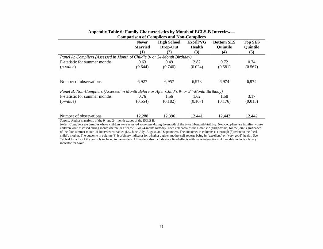
71

Appendix Table 6: Family Characteristics by Month of ECLS-B Interview— Comparison of Compliers and Non-Compliers

Never Married

(1)

High School Drop-Out

(2)

Excell/VG Health

(3)

Bottom SES Quintile

(4)

Top SES Quintile

(5) Panel A: Compliers (Assessed in Month of Child’s 9- or 24-Month Birthday) F-statistic for summer months (p-value)

0.63 (0.644)

0.49 (0.740)

2.82 (0.024)

0.72 (0.581)

0.74 (0.567)

Number of observations

6,927 6,957 6,973 6,974 6,974

Panel B: Non-Compliers (Assessed in Month Before or After Child’s 9- or 24-Month Birthday) F-statistic for summer months (p-value)

0.76 (0.554)

1.56 (0.182)

1.62 (0.167)

1.58 (0.176)

3.17 (0.013)

Number of observations 12,288 12,396 12,441 12,442 12,442 Source: Author’s analysis of the 9- and 24-month waves of the ECLS-B. Notes: Compliers are families whose children were assessed sometime during the month of the 9- or 24-month birthday. Non-compliers are families whose children were assessed during months before or after the 9- or 24-month birthday. Each cell contains the F-statistic (and p-value) for the joint significance of the four summer month-of-interview variables (i.e., June, July, August, and September). The outcomes in columns (1) through (3) relate to the focal child’s mother. The outcome in column (3) is a binary indicator for whether a given mother self-reports being in “excellent” or “very good” health. See Table 4 for a list of the controls included in the models. All models also include state fixed effects with wave interactions. All models include a binary indicator for wave.

Appendix Table 7: OLS and Instrumental Variables Estimates of the Impact of Relative, Non-Relative, and Center-Based Child Care Utilization

Variable

OLS Full (1)

Child FE Full (2)

IV 2SLS

(3) Relative child care (vs. parental care)

0.003 (0.002)

0.007*** (0.003)

-0.049 (0.052)

Non-relative child care (vs. parental care)

0.000 (0.002)

-0.000 (0.003)

-0.155*** (0.049)

Center-based child care (vs. parental care)

0.007*** (0.002)

0.005 (0.003)

-0.146** (0.059)

Child characteristics Y Y Y Family characteristics Y Y Y Family characteristics × wave Y Y Y State fixed effects with wave interactions Y N Y Quarter-of-birth N N N Source: Author’s analysis of the 9- and 24-month waves of the ECLS-B. Notes: Standard errors are displayed in parentheses and are adjusted for within-child clustering. . In columns (1) and (2), a single regression of test scores is estimated on separate binary indicators of relative, non-relative, and center-based child care utilization. In column (3), each cell represents a different regression of test scores on the corresponding child care arrangement. Relative child care is a binary indicator that equals unity if a given child is cared for by any relative inside or outside the child’s home (and equals zero for participation in parent care). Non-relative child care is a binary indicator that equals unity if a given child is cared for by any non-relative inside or outside the child’s home (and equals zero for participation in parent care). Center-based child care is a binary indicator that equals unity if a given child participates in center-based care (and equals zero for participation in parent care). See Table 4 for a list of the controls included in the models. All models include a binary indicator for wave. ***, **, * indicate statistical significance at the 0.01, 0.05, and 0.10 levels, respectively.

73

Appendix 1: Summer Maternal Work Behavior and Child Activities

As stated in the main text, Appendix Tables 2 through 4 attempt to answer two questions about children assessed in the summer and non-months of the ECLS-B. First, it is important to examine whether the rise in parent care is offset by a reduction in maternal employment or other changes in work behavior (e.g., shifting from full- to part-time work, delaying a job search, or working from home). Second, it is important to determine the types of activities in which children are engaged with parents, and in particular, whether parents make higher-quality time investments during the summer.

I first examine whether maternal work activity differs across the summer and non-summer months by regressing various measures of employment on the SUMMER dummy and the remaining controls in equation (4). All work outcomes are specified as binary indicators of different work margins. As shown in Appendix Table 2, mothers interviewed in the summer exhibit work behaviors similar to those interviewed during the non-summer months. Indeed, across all five work margins there is consistent evidence that mothers’ employment does not display seasonal variation. Indeed, mothers interviewed during the summer are not less likely to do any work (versus no work), are not more likely to shift from full- to part-time work, and are not less likely to begin a job search.

Such results suggest that the largest summer-induced reductions in child care utilization may be concentrated among mothers with the most flexible work schedules. Appendix Table 3 investigates this possibility by estimating regressions of NP on interactions between SUMMER and various employment schedules (Panel A) and between SUMMER and various places of employment (Panel B). Results in Panel A indicate that the summer participation “dip” is particularly large among mothers currently looking for work or not in the labor force. The regression estimates imply child care utilization reductions of 18 percent and 17 percent, respectively, for these mothers, while those working full- or part-time experience virtually no change in their summer child care use. A similar pattern emerges in Panel B: mothers with greater employment flexibility—in this case, those working from home—are more likely to stop using non-parental care in the summer compared to those working outside the home or the self-employed. To explore the nature of children’s activities during the summer, I draw on a battery of questions in the ECLS-B that inquire about the frequency with which parents and children read stories, run errands, and play in the yard; visit the zoo and museum; and eat breakfast and dinner together. Some of these activity questions are asked in both waves, while others are asked in only a single wave. All outcomes are measured as binary indicators that equal unity if a given activity occurred within the timeframe allotted in the questionnaire. For each activity, regressions are estimated on interactions between SUMMER and various employment schedules (Panel A) and between SUMMER and various places of employment (Panel B). As shown in Appendix Table 4, it is clear that parental time investments increase in the summer, regardless of mothers’ employment status or place of employment. In addition, many of these investments appear to be high-quality (e.g., visiting the zoo and museums and sharing family meals). There is also evidence that the largest investments are made by mothers with the most flexible work schedules, a pattern consistent with participation “dip” discussed above. For example, mothers currently looking for work or working from home are more likely to read stories to and run errands with the focal child, visit the zoo, and have dinner as a family than mothers in other work categories.