The Impact of Insurance Premium Taxation - uni … · The Impact of Insurance Premium Taxation ......

The Impact of Insurance Premium Taxation

Anna-Maria Hamma

Leibniz Universität HannoverMoritz Hildebrandtb

Mecklenburgische Versicherung

Stefan Weberc

Leibniz Universität Hannover

May 29, 2017d

Abstract

In many countries insurance premiums are subject to an insurance premium tax thatreplaces the common value-added tax (VAT) used for most products and services. Insurancecompanies cannot deduct VAT payed on inputs from premium tax; also corporate buyers ofinsurance cannot deduct premium tax payments from VAT on their outputs. Such deductionswould be allowed, if insurance premiums were subject to VAT instead of insurance tax.

In the current paper, we investigate the impact of the premium tax on insurance companies,insurance holders and government revenues from multiple perspectives. We explicitly comparetax systems with premium tax and tax systems that allow deductions. We find that thecompetitiveness of corporate buyers of insurance, the ruin probabilities of insurance firms andtheir solvency capital are hardly affected by the tax system. In contrast, the tax system hasa significant influence on the cost of insurance, insurance demand, government revenues andthe profitability of insurance firms.

1 Introduction

In many countries insurance premiums are subject to insurance premium tax that replaces thecommon value-added tax (VAT) used for most products and services. This is, for example,mandatory according to EU-law. In contrast to VAT, premium tax does not permit any deduc-tions: first, insurance companies cannot deduct VAT payed on inputs from premium tax; second,corporate buyers of insurance cannot deduct their premium tax payments from VAT on theiroutputs, although the insurance contracts are an input to their production. As a consequence,insurance premium tax leads to a higher taxation than VAT if the same tax rate is applied. Inthe current paper, we investigate the impact of premium tax on insurance companies, insuranceholders and government revenues from multiple perspectives.

Subject to premium tax are insurance premiums only. In the case of insurance companies,these are approximately equal to the total revenues of these firms. VAT – in contrast – is notcharged on revenues, but on the value added which is smaller than revenues.

aInstitut für Mathematische Stochastik, Welfengarten 1, 30167 Hannover, [email protected]

bMecklenburgische Lebensversicherung, Abteilung Mathematik, Platz der Mecklenburgischen 1, 30625 Hannover,email [email protected]

cInstitut für Mathematische Stochastik, Welfengarten 1, 30167 Hannover, [email protected]

dThe authors thank Rainer Skowronek for suggesting the topic of the current paper.This paper should not be reported as representing the views of Mecklenburgische Lebensversicherung. The views ex-pressed in this paper are those of the authors and do not necessarily represent those of Mecklenburgische Lebensver-sicherung.

1

Premium tax rates and VAT rates vary across countries. Tax rates may also be different fordifferent types of products. Information on tax rates for individual countries and products can befound in European Commision (2017), Insurance Europe (2016), and BMJV (2017). In Germanythe VAT rate and the premium tax rate coincide for most types of products and are generallyboth equal to 19%.

In absolute terms, government revenues from VAT are much larger than revenues from pre-mium tax due to a larger tax base. In 2015 VAT revenues in Germany were 159,015 millionEUR – corresponding to 23.6% of total tax revenues; premium tax revenues during the same yearwere equal to 12,419 million EUR, i.e. 1.8% of total tax revenues or 7.8% of VAT revenues, seeBundesfinanzministerium (2016).

On the individual level of both the providers and buyers of insurance, premium tax may leadto higher total tax payments. We quantify this effect in Section 2. As already explained, onthe one hand a provider of insurance cannot deduct VAT paid on input goods from premiumtax. On the other hand commercial buyers of insurance cannot deduct the incurred premiumtax from VAT on their outputs. While Section 2 provides an analysis from the point of view ofindividual tax payers, Section 3 calculates the impact on overall tax revenues. More specifically,a tax system with insurance tax is compared to one in which insurance tax is replaced by VAT. Ifthe VAT rate is unchanged, total tax revenues would decrease by EUR 16 billion. An equivalentVAT rate of 89.2% is computed that leads to the original total tax revenues.

After analyzing the basic differences between VAT and premium tax, we provide in Sections 4 –7 a broader perspective on the topic by comparing the impact of different tax systems on insurancedemand, the competitiveness of corporate buyers of insurance, ruin probabilities of insurancefirms, and solvency capital. Section 4 models corporate buyers of insurance as utility maximizersthat can choose their optimal level of insurance. The total cost of insurance depends on the taxsystem that is implemented. We provide case studies that illustrate potential consequences onthe demand for insurance. These show that a change in the tax system from insurance to value-added tax increases the insurance demand. Section 5 investigates the competitiveness of corporatebuyers of insurance. In contrast to Section 4 it is assumed that the amount of insurance that isbought is constant, but that its cost depends on the tax system. If an insurance tax is replaced bya VAT with the same rate, the costs are effectively reduced. If these savings are completely passedon to the buyer of the output products, the demand for these products increases. This is explicitlyquantified in two numerical case studies. While Section 5 assumes that tax savings are used toreduce the price of output products, Sections 6 and 7 suppose that savings are retained by theinsurance company. In Section 6 we generalize the classical Cramér-Lundberg model by includingtax payments in order to study the impact on ruin probabilities. Finally, Section 7 computes howsolvency capital requirements change that are e.g. implemented under the regulatory frameworkof Solvency II or the Swiss Solvency Test. In summary, we find that the competitiveness ofcorporate buyers of insurance, the ruin probabilities of insurance firms and their solvency capitalare hardly affected by the tax system. In contrast, the tax system has a significant influence onthe cost of insurance, insurance demand, government revenues and the profitability of insurancefirms. Section 8 concludes.

Literature. Holzheu (1997) and Holzheu (2000) suggest an accounting methodology in orderto compute basic quantities that characterize the impact of a premium tax. Sections 2 & 3 buildon this methodology. Our sections are, however, based on current data and constitute a necessaryprerequisite for the other parts of our paper. Straubhaar (2006) provides a qualitative analysis ofthe impact of an increased premium tax that is complemented by a regression analysis in orderto obtain quantitative estimates. Schrinner (1997) qualitatively discusses the impact of premiumtax and provides related accounting figures besides a preliminary economic analysis.

2

2 Impact on Insurance Companies and Insurance Holders

Insurance premium tax and value-added tax lead to different tax expenses related to insuranceservices. To begin with, we provide a descriptive analysis on the basis of aggregate accounting datathat quantifies the impact of different tax systems. Our computations follow the methodologydescribed in Holzheu (1997) & Holzheu (2000), using data from 2011 – 2015 provided in BaFin(2011-2015).

Impact on Insurance Companies. We consider an insurance company with earnings of grosspremiums denoted by π ∈ R. Gross premiums are before the deduction of reinsurance. For thepurpose of our comparisons, we define taxed premiums as the sum of gross premiums π and thetax that is charged from the insurees for their insurance contracts, i.e. either premium tax orvalue-added tax – depending on the (real or hypothetical) tax system that we consider.

We denote the prevailing VAT rate by τVAT ≥ 0. The input of the production of insurancecontracts is always taxed according to VAT. Taxed input1 L and untaxed input L can thus beconverted into each other:

L = (1 + τVAT)L.

We define the rate of input α as the ratio of untaxed input and untaxed gross premiums earned:

α =L

π.

Tax legislation in many countries typically prohibits the deduction of VAT paid on inputsfrom premium tax, but would allow a deduction if instead VAT was also paid on outputs. Theamount that would be deducted in this case equals

L− L = τVATαπ. (1)

We now estimate this quantity that is typically not directly reported by insurance companies.Untaxed inputs can roughly be estimated as gross premiums earned plus capital income minustotal losses and costs including taxes. For Germany, the required data were obtained from theannual reports of Bundesanstalt für Finanzdienstleistungsaufsicht (BaFin).

Example 2.1. On the basis of BaFin-data for the years 2011 – 2015 (see BaFin (2011-2015)),the mean rate of input2 equals α = 5.2%. With τVAT =19%, this implies a difference of untaxedand taxed inputs equal to L− L ≈ 0.99% · π.

Equivalent Value-Added Tax Rate. The current tax system charges VAT on the productioninputs of insurance firms, but premium tax on their outputs, i.e. on insurance contracts. Adeduction of VAT on inputs from premium tax is not permitted. What is the hypothetical VATrate on the value added generated by the insurance contracts that leads to the same tax paymentsas insurance tax? We call this counterfactual VAT the equivalent value-added tax. We stress thatthe VAT rate on all other goods and services remains unchanged in this gedankenexperiment. Wesimply analyze a modified basis of assessment of the tax that is charged on insurance contracts,holding the tax revenue constant. In the case of premium tax, the basis of assessment are thepremiums; in the case of the equivalent VAT, the basis of assessment is the value added generatedby the insurance industry.

We denote the premium tax rate by τPT ≥ 0 and the insurance’s value added before taxes byW . The value added before taxes is estimated as the sum of acquisition costs and administrative

1In this paper, taxed variables are marked with a bar .2Input ratios were estimated on the basis of an aggregated stylized income statement of insurance companies

provided by BaFin. Input ratios were computed for single years, then added and finally averaged over time. Forthe detailed computation we refer to Appendix B.

3

expenses, profits before taxes and changes in equalization provisions and similar provisions. Inorder to account for the fraction of the value added that is indirectly generated by reinsurers’share of gross premiums earned we add the difference between the gross technical result and nettechnical result. From BaFin-data 2011 – 20153 we compute

W ≈ 31.3% · π.

The equivalent value-added tax rate that leads to the same tax revenue can be calculated by thechange of basis of assessment equation,

τVATW = τPTπ ⇔ τVAT = τPT ·π

W.

Example 2.2. For many types of insurance contracts the premium tax rate in Germany equalsτPT = 19%. With π/W ≈ 1/31.3% = 3.19 as calculated above, we obtain an equivalent VAT rateof

τVAT ≈ 60.7%.

Remark 2.3. Value added before taxes varies among different lines of insurance. EquivalentVAT rates are displayed in Table 1.4

Class Value added ratio Equivalent VAT rate

Accident 39% 49%Public liability 37% 51%Car total 21% 89%Defense 37% 51%Fire 35% 55%Household 43% 45%Residential building 32% 59%Credit and guarantee 37% 51%Total 31% 61%

Table 1: Equivalent VAT rates for different lines of insurance.

Impact on Insurance Holders. Next, we consider a hypothetical tax system in which VATcan be deducted from premium tax, and premium tax from VAT. In this case, the basis ofassessment of the premium tax are the gross premiums earned, but counterfactual deductions areadmissible. We assume that all tax savings are passed to a corporate buyer of insurance contracts.The latter are treated as an input good to the buyer’s production, allowing for a deduction ofincurred premium tax from VAT on outputs of the corporate customer. Total tax savings canthus be decomposed into two components: a) the VAT on the input goods of insurance firmsdeducted from premium tax, b) premium tax deducted from the VAT on the output goods of thecorporate buyer of insurance.

We compute the size of these tax savings. For this purpose, we denote the total revenue (orbusiness volume) of the corporate insurance holder by U ∈ R and her untaxed cost of insuranceby V ∈ R. The insurance ratio of the company is defined as

β :=V

U∈ [0, 1]. (2)

Lemma 2.4. If VAT and premium tax can be deducted from each other, if taxes on outputs arehigher than on inputs and if all tax savings are passed on to a corporate buyer of insurance, thenthis firm has tax savings of

E = (τVAT α+ τPT)βU. (3)3Value added was calculated for every year, summed up and averaged over time. For the detailed computation

we refer to Appendix B.4For the detailed computation of the quantities we refer to Appendix B.

4

Proof. The savings are given by (1) plus the input tax reduction of the company for insuranceproducts., i.e. E = τVAT αV + τPT V .

Example 2.5. Setting the input ratio to α =5.2% as in Example 2.1 and the insurance ratio toβ =0.5%,5 we obtain

E = 0.1% · U,

i.e. the total savings are only approximately 10 basis points of the business volume of the company.The parameter β depends on the industry sector of the corporate insurance holder. According toSwiss Re, sigma No 5/2012 (sigma (2012), p. 17) it varies between 0.1% and 1.4% for differentUS industries.

3 Impact on Tax Revenues

We will now discuss the impact on total tax revenues, if premium tax is replaced by VAT. First,we compute the modified tax revenues. Second, we calculate an equivalent VAT which leads tothe same total tax revenues. The derivations build on the results of the previous section. Themethodology is motivated by Holzheu (2000), p. 76ff.

Comparison of Tax Revenues. Let Π be the total national untaxed gross insurance premiumsearned, W the total value added before taxes of the corresponding insurance companies, and αtheir input ratio. The tax revenue S related to insurance contracts in a tax system with premiumtax can be split into three parts:

(i) VAT of insurance companies on their inputs: This amount cannot be deducted from pre-mium tax. It can be computed according to eq. (1).

(ii) Premium tax.

(iii) VAT on taxed insurance premiums: The costs of the outputs of corporate buyers of insur-ance are increased by the premium tax. This is implicitly reflected in their prices and leadsto additional value-added tax revenues.

Total tax revenues are given by adding up the three parts:

S = (τVATα+ τPT) ·Π + τVAT · (1 + τPT) ·ΠG.

Here, ΠG denotes the untaxed insurance premiums of corporate holders of insurance. Policies ofprivate customers are included in Π but not in ΠG, since they are not indirectly charged withadditional VAT.

Suppose now that insurance premiums are not subject to a premium tax but to a value-addedtax. In this case, these taxes are fully deductable and double-taxation is avoided. The totalrelevant tax revenue thus amounts to S := τVATW . In particular, if we assume that τPT ≥ τVAT

and W < Π, thenS = τVATW < τPTΠ < S.

Changing the tax system from premium tax to VAT thus leads to lower total tax revenues, if thecorresponding tax rates are equal.

5As a rough approximation of β we use an estimate that is provided in Swiss Re, sigma No 5/2012 (sigma(2012), p. 16) for the US market. Since the main purpose of Example 2.5 is to provide an estimate of the order ofthe impact of a modified tax system on corporate insurance costs, precise knowledge of β is not required.

5

Equivalent Value-Added Tax Rate. As before, we compute an equivalent VAT rate τVAT

that leads to the same tax revenues, but now also incorporates taxes on premium tax paid bycorporate insurance customers. As in the previous section we assume that the VAT rate on allother goods and services remains unchanged in this thought experiment. We only focus on thosetax revenues that are directly related to insurance contracts as explained above.

Lemma 3.1. We denote by g := ΠGΠ the ratio of untaxed corporate insurance premiums over total

untaxed insurance premiums. The equivalent value-added tax rate τVAT is given by

τVAT = (τVATα+ τPT + τVAT(1 + τPT)g) · Π

W.

Proof. The result follows immediately from the condition τVATW = S.

Example 3.2. The average value added before taxes of German insurance firms during the period2011 – 20156 amounts to

W ≈ 31.3% ·Π.

If we assume that the fraction of premiums of corporates is g =35%,7 we obtain for τVAT =τPT = 19% and α = 5.2%8 an equivalent value-added tax rate of

τVAT ≈ 89.2%.

Finally, let us consider a modification of the tax system in which premium tax is replaced byVAT. This would, in particular, imply that both VAT on insurance companies’ inputs and VATon premium tax paid by corporate customers are deductible. For the purpose of illustrating thesize of this effect, we suppose that the German premium tax of 19% is replaced by VAT of 19%.This would decrease total German tax revenues by approximately

S − τVAT · W = (τVATα+ τPT + τVAT(1 + τPT)g − τVAT · 31.3%) ·Π = (27.9%− 5.9%) ·Π = 22% ·Π.

Taking Π ≈ EUR 75 billion (corresponding to German gross premiums earned in 2015), taxrevenues would decrease by approximately EUR 16 billion, if the tax system was changed.

4 Impact on Insurance Demand

The current German premium tax leads to an additional tax burden for insurance contracts. Inthis section we investigate the impact of the tax system on insurance demand. Insurance demandis endogenously modeled in a classical expected utility framework. For proportional insurance,we compute the optimal demand maximizing the expected utility of the policyholder.

Model 4.1 (Insurance Demand). We consider a proportional insurance contract over a fixedtime horizon. The initial wealth of the insurance holder is denoted by w > 0. Over the timeinterval, the insurance holder incurs a random loss X ∈ L1(R+) where L1(R+) denotes the spaceof integrable real-valued random variables on some probability space (Ω,F , P ) with values in R+.The insurance contract is characterized by the parameter ν ∈ [0, 1] which is the fraction of theloss that is covered by the insurance. The premium for full insurance is π ∈ R+; the premium forpartial insurance of a fraction ν of the loss X is ν · π.

6Compare Footnote 3.7This number quantifies the fraction for Germany in 2010 according to sigma (2012), p. 10, Table 3. 35% of

the total non-life premium income was generated by corporate buyers of insurance contracts.8See Example 2.1.

6

The terminal endowment of the insurance holder as a function of ν is

Xν = w −X + ν(X − π) = (1− ν)(w −X) + ν(w − π).

Buyers of insurance can choose the fraction ν according to their preferences. This fraction iscomputed as the solution to a utility maximization problem of the policyholder, see e.g. Chapter2 in Föllmer & Schied (2011).

As a first example, we consider a Bernoulli utility function with constant absolut risk aversion(CARA). This function has the form uκ1(x) = 1 − e−κx with κ > 0. Another example is aBernoulli utility function with hyperbolic absolut risk aversion (HARA), given by uλ2(x) = 1

λxλ

for λ ∈ (0, 1). The limiting case λ = 0 corresponds to logarithmic utility. The Arrow-Pratt-coefficients of absolute risk aversion are κ for uκ1 and the hyperbolic function x 7→ (1 − λ)/x foruλ2 , explaining the terminology. In the case of HARA utility we will always assume that X ≤ w,for logarithmic utility X < w.

Problem 4.2 (Expected Utility Maximization). Let S ⊆ R be convex and assume that u : S → Ris a Bernoulli utility function, i.e. a function that is strictly concave, strictly increasing andcontinuous on S. Suppose that the support supp Xν is contained in S and that u(Xν) is integrablewith respect to P for all ν ∈ [0, 1]. Then the optimal insurance contract is characterized by themaximizer ν∗ ∈ [0, 1] of the expected utility

ν 7→ E [u(Xν)] .

A necessary condition for an interior solution ν ∈ (0, 1) is given by the first order condition

∂

∂νE [u(Xν)] = 0.

We compare different tax regimes for two examples of loss distributions, a Bernoulli and a Gammadistribution. In the case of a Bernoulli distribution, we assume that a loss x > 0 occurs withprobability p ∈ (0, 1), and no loss with probability 1 − p, i.e. X ∼ Ber(x, p). For HARA utilitywe assume that x ≤ w, for logarithmic utility x < w. For a Gamma distribution with parametersξ, µ > 0 and density

fξ,µ(x) =µξ

Γ(ξ)xξ−1 e−µx 1(0,∞)(x), x ∈ R,

we use the notation Γ(ξ, µ). Note that Γ(·) denotes the ordinary gamma function. The Gammadistribution with unbounded support will only be considered in the case of CARA utility.

Remark 4.3. The following result is a simple consequence of Föllmer & Schied (2011), Propo-sition 2.39: Let u : dom u → R be a Bernoulli utility function. We assume that R+ ⊆ dom u,X ≤ w and π ≤ w. Then the following assertions hold:

(a) We have ν∗(π) = 1 if π ≤ E[X], and ν∗(π) > 0 if π ≤ w − cX , where cX is the certaintyequivalent given by the equation E[u(X)] = u(cX).

(b) If u is differentiable, thenν∗(π) = 1 ⇔ π ≤ E[X]

and

ν∗(π) = 0 ⇔ π ≥ w − E[(w −X)u′(w −X)]

E[u′(w −X)].

If π < w − E[(w−X)u′(w−X)]

E[u′ (w−X)], then ν∗(π) > 0.

7

A risk-averse buyer purchases full insurance, if and only if the premium does not exceed theexpected loss. Insurers will, however, always charge premiums that are larger in order to avoidruin. In this case, full insurance is never optimal.For the special case of Bernoulli-distributed random variables Schrinner (1997) discussed

ν∗(π)

= 1, if π ≤ E[X],

< 1, if π > E[X],

in the context of premium tax. He argued that higher premium taxes lead to higher premiums andtherefore to a larger deviation of the premium from the expected loss, which results in less demandfor insurance.

Theorem 4.4. The solutions to Problem 4.2 for specific utility functions and loss distributionsare as follows:

(i) CARA-utility: Consider the Bernoulli utility u(x) = uκ1(x), κ > 0.

• Assume that losses are Bernoulli-distributed, i.e. X ∼ Ber(x, p). Then the optimalinsurance contract is characterized by

ν∗(π) =

0, π ≥ pxeκx

1−p+peκx ,

1− 1κx ln

(1p−1

xπ−1

), pxeκx

1−p+peκx > π > px,

1, px ≥ π.

• Assume that losses are Gamma-distributed, i.e. X ∼ Γ(ξ, µ), and assume that κ < µ.Then the optimal insurance contract is given by

ν∗(π) =

0, π ≥ ξ

µ−κ ,

1 + ξπκ −

µκ ,

ξµ−κ > π > ξ

µ ,

1, ξµ ≥ π.

(ii) HARA-utility: Consider the Bernoulli utility u(x) = uλ2(x), λ ∈ (0, 1). We set ζ = 11−λ .

• Assume that losses are Bernoulli-distributed, i.e. X ∼ Ber(x, p). We suppose that0 < x ≤ w. Then the optimal insurance contract is

ν∗(π) =

0, π ≥ pxw1−λ

pw1−λ+(1−p)(w−x)1−λ,

πζ(1−p)ζ(x−w)+pζ(x−π)ζwπζ(1−p)ζ(x−π)+pζ(x−π)ζπ

, pxw1−λ

pw1−λ+(1−p)(w−x)1−λ> π > px,

1, px ≥ π.

(iii) Logarithmic utility: Consider the logarithmic utility u02(x) = log(x), i.e. the limiting

case of HARA-utility for λ = 0.

• Assume that losses are Bernoulli-distributed, i.e. X ∼ Ber(x, p). We suppose that0 < x < w. Then the optimal insurance contract is characterized by

ν∗(π) =

0, π ≥ pxw

w+x(p−1) ,π(w−x)−px(w−π)

π(π−x) , pxww+x(p−1) > π > px,

1, px ≥ π.

Proof. See Section A.

8

In order to gauge the effect of a modified tax on insurance demand, we now compute themodification of the effective premiums for different tax systems.

Lemma 4.5. We denote the taxed premium in a system with premium tax by πPT. Assume nowthe counterfactual situation that VAT and premium tax can be deducted from each other and thatat the same time all tax savings are passed to a corporate buyer of insurance. In this case, theeffective premium equals

πVAT = γ · πPT, γ := 1− τVATα+ τPT

1 + τPT,

where α denotes the input ratio.

Proof. The result follows from πVAT = πPT − E where tax savings E are computed according toequation (3) with πPT = (1 + τPT)βU .

Example 4.6. For an input ratio α = 5.2% and τVAT = τPT =19%, we obtain γ ≈ 0.832, i.e. theeffective premium reduces to 83.2% of the original premium, if deduction is permitted.

Before we can analyze the impact of alternative tax systems on demand, we need to specify howpremiums are calculated net of taxes. We focus on two examples of classical premium principles,namely the expected value principle and the standard deviation principle, see e.g. Chapter 12in Schmidt (2009). We also investigated the semi-standard deviation principle which leads tosimilar results as the standard deviation principle; for this reason it is not included in the casestudies below. However we provide the corresponding formulas. Untaxed premiums with safetyloading δ > 0 are given in Table 2 for the considered loss distributions. Note that Γ(·, ·) denotesthe upper incomplete gamma function. Adjusting tax payments, optimal insurance contracts canfinally be computed according to Theorem 4.4.

Premium Principle X ∼ Ber(x, p) X ∼ Γ(ξ, µ)

Expected Value Principle px(1 + δ) ξµ(1 + δ)

Standard Deviation Principle px(

1 + δ√

1−pp

)ξµ

(1 + δ 1√

ξ

)Semi-Standard Deviation Principle px

(1 + δ 1−p√

p

)ξµ

(1 + δ 1

ξ

√1

Γ(ξ)(ξξ e−ξ + ξ Γ(ξ, ξ)))

Table 2: Computation of untaxed premiums.

The following examples analyze the impact of different tax systems on insurance demand. Inall case studies we assume τPT = 19% and γ = 0.832 according to Example 4.6.

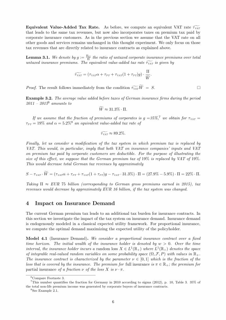
Example 4.7. In the first numerical example, we consider losses X ∼ Ber(x, p) and an insureewith CARA-utility u(x) = uκ1(x), κ > 0. We choose p = 0.1 and vary x. Risk aversion is set toκ = 0.3, and the safety loading equals δ = 0.4.

Figure 1 displays optimal insurance contracts ν∗ for the two different tax systems. In the caseof CARA-utility, these do not depend on the initial endowment of the insuree. As expected, ifdeduction is permitted, the demand for insurance is increased. The difference in demand initiallyincreases for small loss sizes x and decreases towards a small level for larger loss sizes. ComparingFigures (a) and (b), we observe similar shapes of the functions for both premium principles. Dueto higher premiums for the standard deviation principle, the optimal demand for insurance issmaller than in the case of the expected value principle.

9

0 5 10 15 20 25 30 350

0.1

0.2

0.3

0.4

0.5

0.6

0.7

0.8

0.9

1

0

0.1

0.2

0.3

0.4

0.5

0.6

0.7

0.8

0.9

1

Dif

fere

nce

VATInsurance TaxDifference

(a)

0 5 10 15 20 25 30 350

0.1

0.2

0.3

0.4

0.5

0.6

0.7

0.8

0.9

1

0

0.1

0.2

0.3

0.4

0.5

0.6

0.7

0.8

0.9

1

Dif

fere

nce


(b)

Figure 1: Insurance demand in Example 4.7 for expected value and standard deviation principle.

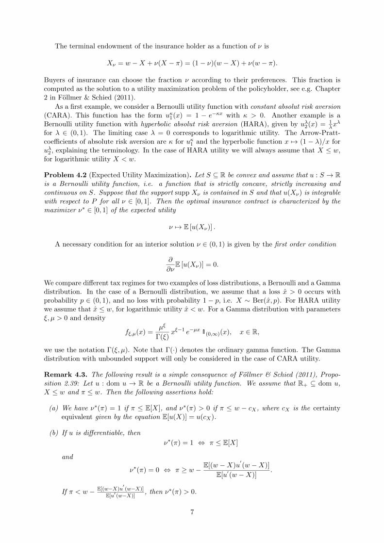
Example 4.8. In the second numerical example, we consider losses X ∼ Γ(ξ, µ) and an insureewith CARA-utility u(x) = uκ1(x), κ > 0. We choose ξ = 1 and vary 1/µ. Risk aversion is againset to κ = 0.3, and the safety loading equals δ = 0.4.

Figure 2 displays optimal insurance contracts ν∗ for the two different tax systems. Again, ifdeduction is permitted, the demand for insurance is increased. The difference in demand is zerofor small expected loss sizes 1/µ ≤ 0.92, increases for 1/µ ∈ (0.92, 1.33), and decreases for largerlosses.

0.5 1 1.5 2 2.5 30

0.1

0.2

0.3

0.4

0.5

0.6

0.7

0.8

0.9

1

0

0.1

0.2

0.3

0.4

0.5

0.6

0.7

0.8

0.9

1

Dif

fere

nce


(a)

0.5 1 1.5 2 2.5 30

0.1

0.2

0.3

0.4

0.5

0.6

0.7

0.8

0.9

1

0

0.1

0.2

0.3

0.4

0.5

0.6

0.7

0.8

0.9

1

Dif

fere

nce


(b)


Example 4.9. In the third numerical example, we consider losses X ∼ Ber(x, p) and an insureewith HARA-utility u(x) = uλ2(x), λ ∈ (0, 1). We choose p = 0.1 and vary x. We set λ = 0.2. Thesafety loading equals δ = 0.01. Initial wealth is w = 300.

Figure 3 displays optimal insurance contracts ν∗ for the two different tax systems. Again, weobtain that the demand for insurance is increased, if deduction is permitted. The difference indemand is large for small loss sizes x and decreases for larger losses. It remains larger than 0.2for all values of x in the case of the expected value principle resp. for all values of x ≥ 10.2 inthe case of the standard deviation principle.

10

0 50 100 150 200 250 3000

0.1

0.2

0.3

0.4

0.5

0.6

0.7

0.8

0.9

1

0

0.1

0.2

0.3

0.4

0.5

0.6

0.7

0.8

0.9

1

Dif

fere

nce


(a)

0 50 100 150 200 250 3000

0.1

0.2

0.3

0.4

0.5

0.6

0.7

0.8

0.9

1

0

0.1

0.2

0.3

0.4

0.5

0.6

0.7

0.8

0.9

1

Dif

fere

nce


(b)


Example 4.10. Finally, we consider the same situation as in Example 4.9, but keep x = 280fixed and vary λ. Risk aversion decreases with increasing λ. Figure 4 displays optimal insurancecontracts ν∗ for the two different tax systems. With VAT, insurance demand stays close to 1 forsmall values of λ. Premium tax leads to a higher cost of insurance, and insurance demand issignificantly lower. In the case of premium tax, insurance demand decreases to 0 as risk aversiongoes to 0, i.e. λ approaches 1. In the case of VAT, this effect occurs only if premiums are computedaccording to the standard deviation principle.

0 0.2 0.4 0.6 0.8 10

0.1

0.2

0.3

0.4

0.5

0.6

0.7

0.8

0.9

1

0

0.1

0.2

0.3

0.4

0.5

0.6

0.7

0.8

0.9

1

Dif

fere

nce


(a)

0 0.2 0.4 0.6 0.8 10

0.1

0.2

0.3

0.4

0.5

0.6

0.7

0.8

0.9

1

0

0.1

0.2

0.3

0.4

0.5

0.6

0.7

0.8

0.9

1

Dif

fere

nce


(b)


In summary, our case studies show that the tax system may have a substantial impact oninsurance demand of corporate insurance customers. The size of this effect depends on the lossdistribution and the utility of the insurance customer, in particular on the size of potential lossesand the risk aversion of the insuree.

5 Impact on Competitiveness

The current tax system in Germany with premium tax does not allow that premium tax andVAT are deducted from each other. If such deductions were permitted, as, for example, in an

11

hypothetical tax system that charges VAT on insurance contracts (instead of premium tax),overall tax payments would be reduced.

Consider a corporate insurance client. We compare two tax systems: a realistic tax systemwith premium tax, and a counterfactual tax system that permits the full deduction of VAT andpremium tax from each other. We assume that the resulting tax savings lead to a reduction ofthe sales prices of the corporate insurance customer. The reduced prices increase the relativecompetitiveness of a domestic firm that benefits from a modified tax system in contrast to itsinternational competitors.

We design a stylized model that captures this effect and allows its quantification. There aretwo firms that produce different goods i = 1, 2 that they sell for prices pi, i = 1, 2. We assumethat demand for the two goods in the economy is the solution to a utility maximization of arepresentative consumer.

Problem 5.1 (Utility Maximization). The utility function of the representative consumer withbudget w ∈ R+ is denoted by u : X → R, X = R+ × R+. The consumer’s demand x∗ = (x∗1, x

∗2)

solves her utility maximization problem

x∗ ∈ argmaxx∈R2+u(x1, x2)

subject to her budget constraintp1x1 + p2x2 = w.

The following preliminary lemma computes the price reduction when the tax system is changed.

Lemma 5.2. Let α be the rate of input of insurance companies, and let β be the insurance ratioof company 1 as defined in equation (2). If company 1 is a domestic company, a modification ofthe domestic tax system, as described in Lemma 2.4, decreases the price of its product by θα,β ·p1,where

θα,β := (τVATα+ τPT)β,

and p1 denotes the original price with premium tax. I.e. the unit price decreases to p1 = (1 −θα,β) · p1.

Proof. We have θα,β = EU where U is the revenue or business volume of the company. Now, the

result follows from (3).

In two case studies, we will now illustrate how a modification of the tax system may changeproduct demand. In the first example, the representative consumer has a utility function ofCobb-Douglas type, in the second with constant elasticity of substitution.

5.1 Cobb-Douglas Utility Function

We recall that a Cobb-Douglas Utility Function has the form

ua(x1, x2) := xa1x1−a2 , a ∈ (0, 1).

Solving the optimization problem 5.1, one obtains the solution

x(a)1 =

aw

p1, x

(a)2 =

(1− a)w

p2.

We compare the change in competitiveness of a domestic and a foreign firm, if the domesticsystem is changed as described before. For this purpose, we assume that company 1 is domesticand company 2 foreign. The price of the product of company 2 is p2 and fixed, but the price ofthe product of company 1 is a function of the domestic tax system.

12

Lemma 5.3. Let p1 be the original price of product 1 and x(a)1 the corresponding demand. Suppose

that p1 is the price of product 1 after modifying the tax system, see Lemma 5.2, and x(a)1 the

corresponding demand. Setting ∆x(a)1 = x

(a)1 − x

(a)1 , we obtain:

∆x(a)1

x(a)1

=θα,β

1− θα,β.

Proof. This is an application of Lemma 5.2 to the solution of the optimization problem.

The relative shift in demand does neither depend on the available budget w nor the preferenceparameter a.

Example 5.4. Taking the numbers from Example 2.5, we compute θα,β ≈ 0.1%, thus

∆x(a)1

x(a)1

≈ 0.1%, ∀a ∈ (0, 1).

The price of the product of the domestic company and its competitiveness is almost not affected bya modification of the tax system. The reason is that the insurance ratio of companies is typicallysmall. In addition, the rate of input of insurance companies is not very large.

Example 5.5. Insurance contracts are an input to the production of goods. Their contributionvaries across different industry sectors and so does the effect of a modification of the tax systemon production costs and product prices. Suppose that the input ratio is set to α =5.2% as inthe previous example. Insurance ratios for different US industry sectors are based on a survey ofMarketStance and were obtained from sigma (2012) (p. 17). The data are displayed in Table 3.

Again, θα,β and ∆x(a)1

x(a)1

are computed according to our model. In all cases, the effects are very

small.

Premium/Business Vol. Saving/Business Vol. Shift in DemandIndustrial Sector β in % θα,β in % ∆x

(a)1 /x

(a)1 in %

Mining 0.80 0.16 0.16Construction 1.31 0.26 0.26Manufacturing 0.31 0.06 0.06Transport, communication, 1.21 0.24 0.24utilities

Retail trade 0.36 0.07 0.07Wholesale trade 0.14 0.03 0.03Financial 0.38 0.08 0.08Services 0.70 0.14 0.14

Table 3: Shift in product demand related to industrial sectors.

5.2 Constant Elasticity of Substitution Utility Function

We recall the definition of a utility function with constant elasticity of substitution (CES):

ua,b(x1, x2) :=(axb1 + (1− a)xb2

) 1b,

where a ∈ (0, 1) and b 6= 0. The latter quantity is called the parameter of substitution. Again, wedenote the budget of the consumer by w. The consumer’s optimal demand is

xa,b1 =w (p1/a)−η

aηp1−η1 + (1− a)ηp1−η

2

, xa,b2 =w (p2/(1− a))−η

aηp1−η1 + (1− a)ηp1−η

2

,

where η := 11−b denotes the elasticity of substitution.

13

Lemma 5.6 (Shift in Demand). Let p1 be the original price of product 1 and xa,b1 the correspondingdemand. Suppose that p1 is the price of product 1 after modifying the tax system, see Lemma 5.2,and xa,b1 the corresponding demand. Setting ∆xa,b1 = xa,b1 − x

a,b1 , we obtain:

∆xa,b1

xa,b1

= (1− θα,β)−ηaη p1−η

1 + (1− a)η p1−η2

(1− θα,β)1−η aη p1−η1 + (1− a)η p1−η

2

− 1.

Proof. This is an application of Lemma 5.2 to the solution of the optimization problem.

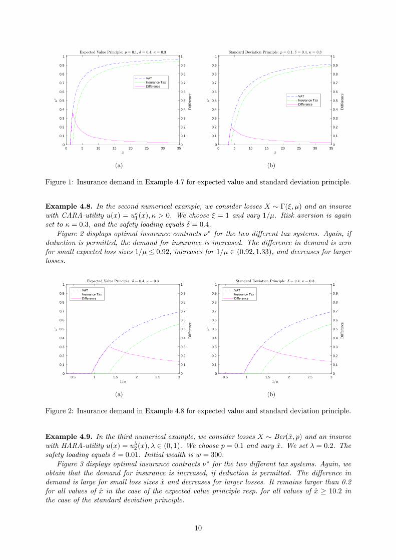
In contrast to a Cobb-Douglas utility, the relative demand shift depends on the parametersof the utility and the price level of the products in the case of CES-utility. The impact of theseinputs on demand is illustrated in Figure 5 for the parameter values given in Table 4.

Saving: θα,β = 0.1%Share Parameter: a ∈ (0, 1)Price of Product 1: p1 = 1Price of Product 2: p2 ∈ [0, 2]

Table 4: Parameters for case studies with CES utility function.

In particular, we consider different parameters of substitution b and elasticity of substitutionη = 1/(1−b). For η > 1 the products are gross substitutes, for η < 1 they are gross complements.We fix p1 = 1 and vary η, a and p2. The resulting relative demand shifts are displayed in Figure5. In case of gross substitutes (η > 1) the increase in demand caused by the price change is, ofcourse, higher than in case of gross complements. The effect is, however, in all cases very small.

0 0.5 1 1.5 20

0.5

1

1.5

2

2.5

310 -3

0 0.5 1 1.5 20

0.5

1

1.5

2

2.5

310 -3

0 0.5 1 1.5 20

0.5

1

1.5

2

2.5

310 -3

0 0.5 1 1.5 20

0.5

1

1.5

2

2.5

310 -3

= 1/10 = 1/2

= 10/11 = 2

= 10

Figure 5: Relative shift in demand with CES utility functions.

All case studies clearly indicate that the international competitiveness (in terms of productpricing) of corporate insurees is almost not affected by the difference of premium tax and VAT.

6 Impact on Ruin Probability

In this section we investigate the impact of the premium tax on the ruin probability of insurancecompanies and compare the results to other models of taxation. For this purpose, we extend

14

the classical Cramér-Lundberg model by including taxes and compute relative changes in ruinprobabilities for different systems of taxation. A detailed review on ruin theory can be found inAsmussen & Albrecher (2010).

Let (Ω,F , P ) be a probability space. We consider a family of risk processes of insurancecompanies (Rwt )t≥0 enumerated by the initial wealth Rw0 = w ∈ R. The ruin probability of thesecompanies is a function of initial wealth:

ψw(π) := P

(inft≥0

Rwt < 0

).

For later reference, we also emphasize the dependence on the premium rate.

6.1 The Cramér-Lundberg Model

In the current section we recall the classical Cramér-Lundberg model and its basic definition, seeChapter IV in Asmussen & Albrecher (2010).

Model 6.1 (Cramér-Lundberg). Denote the initial capital of the insurance company by w ∈ Rand its premium rate by π ∈ R. Insurance losses are modeled by a compound Poisson process(∑Nt

k=1Xk)t≥0 where individual losses (Xk)k∈N are identically distributed with law B, jointly in-dependent and independent of the Poisson process (Nt)t≥0 with intensity ϑ > 0. The risk processin the Cramér-Lundberg model is given by

Rwt = w + πt−Nt∑k=1

Xk.

Wald’s equation and the strong law of large numbers imply 1t

∑Ntk=1Xk −−−→

t→∞ϑE[X1] =: r

almost surely.If individual losses X1, X2, . . . are exponentially distributed with parameter ι > 0, i.e. Xi ∼

Exp(ι), the ruin probability ψw(π) can be explicitly determined. We cite the following well-knowntheorem (Corollary 3.2, Chapter IV, Asmussen & Albrecher (2010)).

Theorem 6.2 (Exponential Loss-Distribution). Consider the Cramér-Lundberg model with pre-mium rate π = 1 and exponentially distributed losses (Xi)i∈N with parameter ι > ϑ. Then theruin probability of the insurance company is ψw(1) = re−(ι−ϑ)w, r = ϑ

ι .

Notation. If limw↑∞ψw(1)ϕw(1) = 1, we write ψw(1) ∼ ϕw(1). Hence, in the limit the functions are

approximately equal in a relative sense.

For arbitrary loss distributions an approximation of the ruin probability is available (ChapterIV, Theorem 5.3, Asmussen & Albrecher (2010)).

Theorem 6.3 (Cramér-Lundberg Approximation). Consider the Cramér-Lundberg model withpremium rate π = 1. Let B(s) be the moment generating function of B, and assume that theCramér-Lundberg coefficient l, i.e. the solution to the Lundberg-equation B[l] = 1 + l

ϑ , exists.Setting C = 1−r

ϑB′[l]−1, we have as w →∞:

ψw(1) ∼ Ce−lw.

Sensitivity of Ruin Probability. Sensitivities with regard to the premium rate are usefultools for the analysis of the impact of the tax system on the ruin probability. For this purpose weassume from now on that the Cramér-Lundberg coefficient l exists and cite results from Asmussen& Albrecher (2010), Chapter IV (Proposition 9.2 & 9.4).

15

Theorem 6.4 (Sensitivity with regard to π and ϑ).In the Cramér-Lundberg model we have

∂ψw

∂π(1) = −ϑ∂ψ

w

∂ϑ(1),

∂ψw

∂ϑ(1) ∼ we−lw lC2

ϑ(1− r)

as w →∞ where l and C are defined as in Theorem 6.3.

Corollary 6.5. For the ruin probability in the Cramér-Lundberg model we have

∂ψw

∂π(1) ∼ −we−lw lC2

1− r,

∂ψw

∂π(1)

/ψw(1) ∼ −w lC

1− r

as w →∞ .

6.2 The Cramér-Lundberg Model with Taxes

We extend the model and add taxes.

Model 6.6 (Cramér-Lundberg Model with Taxes). Let τ ∈ [0, 1] be a constant tax rate that ischarged on the gross premium income π ∈ R. We denote taxed premiums by π = (1 + τ) · π. Weassume that the realized tax charged on the insurer’s input costs L ∈ R is given by the tax rate ετwhich we represent as a fraction ε ∈ [0, 1] of the premium tax rate τ ∈ [0, 1]. The term realizedtax refers to the tax on inputs minus deductions that are allowed. The costs L do not includeinsurance payments due to losses. The after-tax risk process is

Rw,τ,εt = w +

[π

1 + τ− (1 + ετ)L

]t−

Nt∑k=1

Xk.

The effective insurance premium (after subtracting all expenses and taxes) is

πτ,ε :=π

1 + τ− (1 + ετ)L.

The model allows to mimic different tax systems.

(i) For τ = τPT = τVAT and ε = 1 we obtain a tax system with premium tax in which VAT isapplied to inputs but cannot be deducted from the premium tax payments. This capturesthe current German tax system, if we choose τ = 19%.

(ii) For τ = τVAT and ε = 0 we obtain a counterfactual tax system in which premium tax isreplaced by VAT. In this case, VAT paid on inputs is fully deductable from VAT paid oninsurance premiums.

(iii) Suppose that we are given a tax system with premium tax and VAT as in (i), i.e. τ =τPT = τVAT and ε = 1. As in Example 2.2, we consider a counterfactual tax system (ii) inwhich premium tax is replaced by VAT. We assume that VAT paid on value added of theinsurance firm in the new tax system is equal to insurance tax revenues in the original taxsystem. Moreover, we hold π constant. We denote the modified quantities with a tilde. Inthis case, τ = τVAT = τPT · π

Wand ε = 0 where W is the value that the insurance company

adds to its inputs by producing the insurance contract, see Section 2. The modified taxedpremium rate is given by π = (1 + τ) · π > (1 + τPT) · π. We implicitly assumed that thehigher tax on the premium is payed by the insuree. The financial situation of the insuranceis thus improved in this case, since it can take advantage of tax deductions.

16

(iv) Suppose that we are in a counterfactual tax system (ii). We can extend the arguments in(iii) to construct a corresponding tax system with premium tax. We assume that insurancetax revenues in the new tax system are equal to VAT paid on value added of the insurancefirm in tax system (ii). Moreover, we hold π constant. In this case, the premium tax rateneeds to be adjusted, i.e. τ = τPT = τVAT · Wπ and ε = 1. The modified taxed premiumrate is given by π = (1 + τ) · π < (1 + τVAT) · π. This describes the opposite scenario to thesituation in (iii). The modification of the tax system leads to a higher tax burden of theinsurance company, since tax deductions are no longer possible. The benefits are in thiscase transferred to the insurance customers.

The risk process is a function of the tax parameters τ and ε. We will now investigate howruin probabilities depend on the tax system. In contrast to the examples (iii) and (iv) above wenow keep π fixed instead of π. This implies, in particular, that a modified tax rate on premiumsalters the financial resources and ruin probabilities of the insurance company.

Corollary 6.7. We consider the Cramér-Lundberg model with taxes as described in Model 6.6.The taxed premium rate π and the insurer’s input costs L are assumed to be constant. Wefurther suppose that the effective premium without taxes π − L is normalized to 1. Let ψw be theruin probability function in the original Cramér-Lundberg model 6.1. Then the ruin probability inModel 6.6 with tax parameters τ and ε is given by ψw(πτ,ε). A linear approximation of the relativedeviation of the ruin probability with taxes from the ruin probabilities without taxes exhibits thefollowing asymptotic behavior for w →∞:

ψw(πτ,ε)− ψw(π0,0)

ψw(π0,0)

(πτ,ε ≈ π0,0 = π−L = 1)≈ (πτ,ε−π0,0)·∂ψ

w

∂π(1)

/ψw(1) ∼

(εL+

1

1 + τπ

)τw

lC

1− r

Proof. The linear approximation is given by (πτ,ε − π0,0) · ∂ψw

∂π (1)/ψw(1). Its first factor equals

π

1 + τ− (1 + ετ)L+ L− π = −

(εL+

1

1 + τπ

)τ.

Its second factor was analyzed in Corollary 6.5.

If losses X1, X2, . . . are exponentially distributed with parameter ι > 0 we can refine the linearapproximation on the basis of Theorem 6.2 by applying Theorem 6.4:

(πτ,ε − π0,0) · ∂ψw

∂π(1)

/ψw(1) =

(εL+

1

1 + τπ

)τ (1 + ϑw) . (4)

Figure 6 displays the linear approximation of the relative deviation of the ruin probability withtaxes from the ruin probabilities without taxes for both systems, i.e. premium tax (ε = 1, (i))and VAT (ε = 0, (ii)), for varying tax rates τ .

The required parameters are chosen as follows: We consider the extended Cramér-Lundbergmodel 6.6 with Xi ∼ Exp(ι) , i ∈ N. We set π0,0 = π − L = 1 and w = 43.5%π.9 From theconstraints π0,0 = π − L = 1 and L = απ we deduce π = 1

1+τ−α and hence π = 1+τ1+τ−α and

L = 1+τ1+τ−α − 1. Setting the mean rate of input α = 5.2% as in Example 2.1 and the intensity

ϑ = 1.5, we can use formula (4) to analyze the relative change in ruin probabilities. In general,the higher the tax rate τ the higher the probability of ruin compared to a system without taxes.As expected, the increase of ruin probabilities is stronger in a tax system with premium tax. Achange of the tax system from type (i) to type (ii) would thus reduce the probability of ruin.

9 According to BaFin (2011-2015), Issue 2015, p. 158, Table 520 equity capital of non-life insurance firms inGermany in 2015 was 43.5% of gross premium income.

17

0 0.1 0.2 0.3 0.4 0.5 0.6 0.7 0.8 0.9 10

0.1

0.2

0.3

0.4

0.5

0.6

0.7Insurance Tax SystemVAT System

Figure 6: Relative shift in ruin probability compared to a system without taxes.

In a tax system like in Germany with both VAT and premium tax at 19% the ruin probabilityis increased by approximately 27.63% compared to a system without taxes according to our casestudy. In contrast, if a deduction was allowed, the probability would be increased by only 26.27%.The difference between these numbers is 1.36%. These quantities are all relative changes of theruin probabilities. In absolute terms, annual ruin probabilities of real insurance companies arelimited by regulatory standards. Solvency II, for example, restricts annual ruin probabilities to atmost 0.5%. Otherwise, companies face serious interventions of the regulator. As a consequence,absolute changes of ruin probabilities due to a modified tax system would be extremely moderate– on the order of 1 basis point.

7 Impact on Solvency Capital Requirement

As explained in the previous sections, a premium tax generates more tax revenues than VAT, ifboth tax rates are equal. We now compare these two alternative tax systems from the point ofview of solvency capital requirements. For this purpose, we assume that insurances keep theirtaxed insurance premiums constant, but retain the tax savings that accrue when premium tax isreplaced by VAT. Obviously, the solvency capital requirement is then decreased by this amount,and insurance companies can distribute all tax savings to their shareholders. If this occurs, riskwill be back at its original level. In the current section we review the notion of solvency capitalrequirements and explain in detail why the distribution of dividends to shareholders may beincreased.

To this end, we review the basic definition of distribution-based monetary risk measures.These include all risk measures that are typically used in practice. For a detailed exposition onthe subject we refer to Artzner, Delbaen, Eber & Heath (1999), Föllmer & Schied (2011), andFöllmer & Weber (2015).

Definition 7.1. Let (Ω,F , P ) be a probability space, and X a vector space of random variableson Ω that contains the constants. We identify random variables that are P -almost surely equal.A mapping ρ : X → R is called a monetary risk measure on X , if ρ(X) = ρ(Y ) for X = YP -almost surely and if ρ satisfies the following properties:

18

(i) Monotonicity: If X ≥ Y P -almost surely, then ρ(X) ≤ ρ(Y ).(Better payoff profiles are less risky.)

(ii) Cash-invariance: If m ∈ R, then ρ(X +m) = ρ(X)−m.(Adding a fixed amount m to the risky position decreases the risk exactly by this amount.)

The risk measure ρ is called distribution-based, if ρ(X) = ρ(Y ) whenever X and Y have thesame distribution under P .

Example 7.2. Examples of distribution-based monetary risk measures are Value at Risk (V@R)and Average Value at Risk (AV@R), also called expected shortfall, conditional value at risk, tailvalue at risk, or worst conditional expectation. V@R and AV@R are the basis of the definition ofsolvency capital requirements in Solvency II and in the Swiss Solvency Test, respectively.

(i) Value at Risk at level y ∈ (0, 1) is defined as a quantile:

V@Ry(X) := infm ∈ R |P (X +m < 0) ≤ y.

It is equal to the smallest monetary amount m that needs to be added to the financial positionX such that the probability of a loss does not exceed the level y.

(ii) Average Value at Risk at level y ∈ (0, 1) is the average of the V@Rs below y, i.e.

AV@Ry(X) :=1

y

∫ y

0V@Rc(X) dc.

Under technical conditions, e.g. if X has a continuous distribution, it is equal to the condi-tional expectation of a loss beyond the V@Ry(X).

We will now explain – in a stylised way – how solvency capital requirements are defined. Theevolution of assets, liabilities and capital of an insurance firm can be captured by solvency balancesheets at time horizons that are specified by regulators. The time horizon of Solvency II and theSwiss Solvency Test is one year. Table 5 displays the balance sheet of a company at time t = 0and t = 1.

t = 0

Assets LiabilitiesE0 = A0 − L0

A0

L0

t = 1

Assets LiabilitiesE1 = A1 − L1

A1

L1

Table 5: Balance sheet of an insurance company for different points in time.

The assets are denoted by At, the liabilities by Lt, t = 0, 1. The quantities at time t = 0are known, the quantities at time t = 1 are random variables. The difference between assets andliabilities Et = At−Lt, t = 0, 1, is the net asset value, or capital, of the firm. We set X = E1−E0

for the change of the net asset value over the considered time horizon.The solvency capital requirement (SCR) for Solvency II is defined in the Directive 2009 / 138

/ EC of the European Parliament and of the Council on the taking-up and pursuit of the businessof Insurance and Reinsurance – Solvency II (see European Commission (2009)):

The Solvency Capital Requirement should be determined as the economic capital to beheld by insurance and reinsurance undertakings in order to ensure that ruin occurs nomore often than once in every 200 cases or, alternatively, that those undertakings willstill be in a position, with a probability of at least 99.5 %, to meet their obligations to

19

policy holders and beneficiaries over the following 12 months. That economic capitalshould be calculated on the basis of the true risk profile of those undertakings, takingaccount of the impact of possible risk-mitigation techniques, as well as diversificationeffects.

This definition is specified in terms of condition on the acceptability of E1. An equivalent formu-lation10 provides the definition of the SCR under Solvency II:

P (E1 < 0) ≤ y ⇔ V@Ry(E1) ≤ 0 ⇔ V@Ry(E1 − E0) ≤ E0 ⇔ V@Ry(X) ≤ E0.

Setting SCR := V@Ry(X), the solvency condition of the company becomes

SCR ≤ E0.

An analogous argument holds, if V@R is replaced by any other risk measure ρ.11 The accep-tance set of ρ is the family of positions with non-positive risk, i.e.

Aρ = x ∈ X : ρ(X) ≤ 0.

If we assume again for simplicity that interest rates over a one-year horizon are zero (for thegeneral case see Christiansen & Niemeyer (2014)), setting SCR := ρ(X), we obtain the followingsolvency condition:

E1 ∈ Aρ ⇔ ρ(E1) ≤ 0 ⇔ SCR ≤ E0.

The Swiss Solvency Test chooses AV@R as the basis for the definition of solvency.Let us now return to the original question regarding the impact of the tax system on solvency

capital. In equation (1) we computed the tax savings that accrue if a deduction of VAT paidon inputs was permitted. We assume that these savings of L − L = τVATαπ are retained by theinsurance company. While initial capital E0 remains unchanged, capital E1 at the solvency timehorizon is increased by this amount. This leads to a reduction of the SCR.

Lemma 7.3. We denote by SCR the solvency capital requirement in the original tax system withpremium tax. Assume that the tax system is modified such that a deduction of VAT paid on inputsis permitted. In this case, the solvency capital requirement is reduced to

SCR− τVATαπ.

Proof. Adjusted quantities are labeled with a tilde. The random economic capital at time t = 1becomes E1 = E1 + τVATαπ. We compute

SCR = ρ(X + τVATαπ) = ρ(X)− τVATαπ = SCR− τVATαπ.

Considering the situation in Example 2.1, the reduction of the solvency capital by τVATαπwould amount to 0.99% of gross premium income. The company could increase the dividendpayments to its shareholders by this amount. Government revenues would decrease by the sameamount. The solvency situation of insurance firms would be unchanged in this situation.

10For simplicity, we assume in this paper that interest rates over the one-year horizon are approximately zero.For adjustments on the definition of the SCR if interest rates are non zero see Christiansen & Niemeyer (2014).

11V@R has been criticised in the context of capital regulation, since it neglects losses beyond the V@R and – dueto its lack of coherence – it might mislead investment decisions and asset-liability-management. In addition, incorporate groups it allows “to sweep the downside risk under the carpet”, see Weber (2017).

20

8 Conclusion

We analyzed the impact of premium tax on total tax revenues, insurance demand, competitive-ness of corporate buyers of insurance, ruin probabilities of insurance firms and their solvencycapital requirement. We find that the competitiveness of corporate buyers of insurance, the ruinprobabilities of insurance firms and their solvency capital are hardly affected by the tax system.In contrast, the tax system has a significant influence on the cost of insurance, insurance demand,government revenues and the profitability of insurance firms.

21

A Proof of Theorem 4.4

Proof.

(i) CARA-utility:We first consider the case X ∼ Ber(x, p). We compute

E[uκ1(Xν)] = 1− e−κ(w−νπ)(eκ(1−ν)xp+ 1− p

).

This implies

∂

∂νE[uκ1(Xν)] = κeκ(πν−xν+x−w)

(π(p− 1)eκxν−κx + p(x− π)

).

At the boundary ν = 0 we obtain

∂

∂νE[uκ1(Xν)]|ν=0

= κeκ(x−w)(π(p− 1)e−κx + p(x− π)

).

Thus, ν(π) = 0 is the optimal solution, if and only if

∂

∂νE[uκ1(Xν)]|ν=0

≤ 0 ⇐⇒ π ≥ pxeκx

1− p+ peκx.

At the boundary ν = 1 we obtain ∂∂νE[uκ1(Xν)]|ν=1

= κeκ(π−w)(px− π). Thus, the optimalsolution is ν(π) = 1, iff ∂

∂νE[uκ1(Xν)]|ν=1≥ 0, i.e. π ≤ px. In all other cases, we need to solve

∂∂νE[uκ1(Xν)] = 0, leading to the stated solution. The first order conditions are sufficientdue to the strict concavity.Second, we derive the optimal contract for X ∼ Γ(ξ, µ). In this case,

E [uκ1(Xν)] = 1− e−κ(w−νπ)

(µ

µ− κ(1− ν)

)ξ,

∂

∂νE [uκ1(Xν)] = e−κ(w−νπ)

(µ

µ− κ(1− ν)

)ξ+1(−κµ

)(π(µ− κ(1− ν))− ξ).

The solution can now be derived by analogous arguments as before.

(ii) HARA-utility: Using the same steps as above, the solution is computed, observing

E[uλ2(Xν)

]=

1

λ·(

((1− ν)(w − x) + ν(w − π))λ · p+ ((1− ν)w + ν(w − π))λ · (1− p)),

∂

∂νE[uλ2(Xν)

]= (w − νπ + x(ν − 1))λ−1p(x− π) + (−π)(1− p)(w − νπ)λ−1.

(iii) Logarithmic utility: Again, the solution is derived by analogous arguments, noting

E[u0

2(Xν)]

= log((1− ν)(w − x) + ν(w − π)) · p+ log((1− ν)w + ν(w − π)) · (1− p),∂

∂νE[u0

2(Xν)]

=1

w − νπ + xν − xp(x− π) + (−π)(1− p) 1

w − νπ.

22

B Computations of Section 2

Rate of Input

2015 2014 2013 2012 2011Gross premiums earned π 75,008,740 71,216,091 69,298,052 66,922,556 63,514,681Capital income 7,431,575 7,246,143 7,207,242 7,451,052 6,988,566Investment expenses 1,269,941 923,197 1,010,400 1,098,403 1,740,899Total losses 56,243,800 52,078,719 55,722,781 50,255,508 48,929,622Acquisition costs and administrative expenses 18,921,252 18,083,843 17,594,251 17,113,492 16,486,877Taxes 1,462,200 1,479,200 963,100 1,483,700 1,147,200Input L 4,543,122 5,897,275 1,214,762 4,422,505 2,198,649

Table 6: Computation of input costs in thousands of euros (TEUR).These values are given in Table 540 of the corresponding annual report of BaFin (2011-2015). (Negative) Taxes are disclosedin Table 79 of the same reports.

2015 2014 2013 2012 2011 MeanGross premiums earned 100.00 100.00 100.00 100.00 100.00Capital income 9.91 10.17 10.40 11.13 11.00Investment expenses 1.69 1.30 1.46 1.64 2.74Total losses 75.00 73.10 80.40 75.10 77.00Acquisition costs and administrative expenses 25.20 25.40 25.40 25.60 26.00Taxes 1.95 2.08 1.39 2.22 1.81Rate of Input α 6.07 8.30 1.75 6.58 3.46 5.23

Table 7: Computation of rate of input α as ratio of earned gross premium π.Total losses as well as acquisition costs and administrative expenses can be adopted from Table 540 in the correspondingannual report of BaFin (2011-2015). Other quantities are calculated using Table 6.

Value added

2015 2014 2013 2012 2011Acquisition costs and administrative expenses 18,921,252 18,083,843 17,594,251 17,113,492 16,486,877Profits before taxes 2,548,300 2,587,900 2,135,800 2,472,600 1,986,700Changes in equilization provisions 295,400 684,500 -180,700 858,400 -368,700Gross technical result 4,859,078 5,076,151 -165,970 3,442,647 1,812,497Net technical result 2,931,694 2,908,918 288,506 1,573,496 377,868

Value added W 23,692,336 23,523,476 19,094,875 22,313,643 19,539,506

Table 8: Computation of value added in TEUR.Profits before taxes and (negative) changes in equilization provisions are given in Table 79 of the corresponding annual reportof BaFin (2011-2015). Gross and net technical results can be found in Table 540 of the same reports.

2015 2014 2013 2012 2011 MeanAcquisition costs and administrative expenses 25.20 25.40 25.40 25.60 26.00Profits before taxes 3.40 3.63 3.08 3.69 3.13Changes in equilization provisions 0.39 0.96 -0.26 1.28 -0.58Gross technical result 6.50 7.10 -0.20 5.10 2.90Net technical result 3.91 4.08 0.42 2.35 0.59

Value added Wπ

31.58 33.01 27.60 33.33 30.85 31,28

Table 9: Computation of value added as ratio of earned gross premium π.Acquisition costs and administrative expenses as well as gross technical result can be adopted from Table 540 in the corre-sponding annual report of BaFin (2011-2015). Other quantities are calculated using Table 8 and π in Table 6.

23

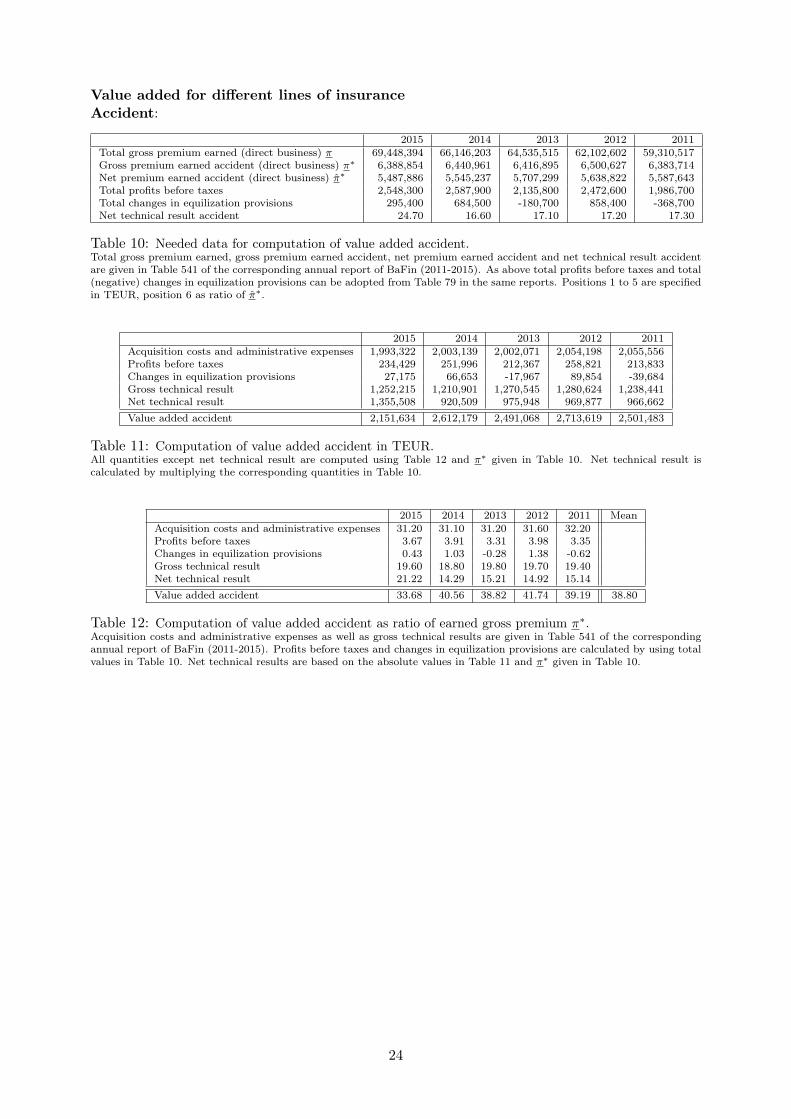
Value added for different lines of insuranceAccident:

2015 2014 2013 2012 2011Total gross premium earned (direct business) π 69,448,394 66,146,203 64,535,515 62,102,602 59,310,517Gross premium earned accident (direct business) π∗ 6,388,854 6,440,961 6,416,895 6,500,627 6,383,714Net premium earned accident (direct business) π∗ 5,487,886 5,545,237 5,707,299 5,638,822 5,587,643Total profits before taxes 2,548,300 2,587,900 2,135,800 2,472,600 1,986,700Total changes in equilization provisions 295,400 684,500 -180,700 858,400 -368,700Net technical result accident 24.70 16.60 17.10 17.20 17.30

Table 10: Needed data for computation of value added accident.Total gross premium earned, gross premium earned accident, net premium earned accident and net technical result accidentare given in Table 541 of the corresponding annual report of BaFin (2011-2015). As above total profits before taxes and total(negative) changes in equilization provisions can be adopted from Table 79 in the same reports. Positions 1 to 5 are specifiedin TEUR, position 6 as ratio of π∗.

2015 2014 2013 2012 2011Acquisition costs and administrative expenses 1,993,322 2,003,139 2,002,071 2,054,198 2,055,556Profits before taxes 234,429 251,996 212,367 258,821 213,833Changes in equilization provisions 27,175 66,653 -17,967 89,854 -39,684Gross technical result 1,252,215 1,210,901 1,270,545 1,280,624 1,238,441Net technical result 1,355,508 920,509 975,948 969,877 966,662Value added accident 2,151,634 2,612,179 2,491,068 2,713,619 2,501,483

Table 11: Computation of value added accident in TEUR.All quantities except net technical result are computed using Table 12 and π∗ given in Table 10. Net technical result iscalculated by multiplying the corresponding quantities in Table 10.

2015 2014 2013 2012 2011 MeanAcquisition costs and administrative expenses 31.20 31.10 31.20 31.60 32.20Profits before taxes 3.67 3.91 3.31 3.98 3.35Changes in equilization provisions 0.43 1.03 -0.28 1.38 -0.62Gross technical result 19.60 18.80 19.80 19.70 19.40Net technical result 21.22 14.29 15.21 14.92 15.14Value added accident 33.68 40.56 38.82 41.74 39.19 38.80

Table 12: Computation of value added accident as ratio of earned gross premium π∗.Acquisition costs and administrative expenses as well as gross technical results are given in Table 541 of the correspondingannual report of BaFin (2011-2015). Profits before taxes and changes in equilization provisions are calculated by using totalvalues in Table 10. Net technical results are based on the absolute values in Table 11 and π∗ given in Table 10.

24

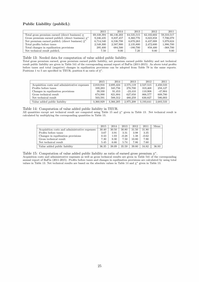
Public Liability (publicL):

2015 2014 2013 2012 2011Total gross premium earned (direct business) π 69,448,394 66,146,203 64,535,515 62,102,602 59,310,517Gross premium earned publicL (direct business) π∗ 9,246,435 8,837,457 8,360,776 8,023,858 7,706,079Net premium earned publicL (direct business) π∗ 6,714,540 6,536,798 6,670,263 6,437,008 5,979,624Total profits before taxes 2,548,300 2,587,900 2,135,800 2,472,600 1,986,700Total changes in equilization provisions 295,400 684,500 -180,700 858,400 -368,700Net technical result publicL 7.50 9.00 7.20 9.80 9.80

Table 13: Needed data for computation of value added public liability.Total gross premium earned, gross premium earned public liability, net premium earned public liability and net technicalresult public liability are given in Table 541 of the corresponding annual report of BaFin (2011-2015). As above total profitsbefore taxes and total (negative) changes in equilization provisions can be adopted from Table 79 in the same reports.Positions 1 to 5 are specified in TEUR, position 6 as ratio of π∗.

2015 2014 2013 2012 2011Acquisition costs and administrative expenses 2,810,916 2,695,424 2,575,119 2,527,515 2,450,533Profits before taxes 339,283 345,756 276,700 319,468 258,127Changes in equilization provisions 39,330 91,453 -23,410 110,908 -47,904Gross technical result 674,990 821,884 627,058 866,577 608,780Net technical result 503,591 588,312 480,259 630,827 586,003Value added public liability 3,360,929 3,366,205 2,975,208 3,193,641 2,683,533

Table 14: Computation of value added public liability in TEUR.All quantities except net technical result are computed using Table 15 and π∗ given in Table 13. Net technical result iscalculated by multiplying the corresponding quantities in Table 13.

2015 2014 2013 2012 2011 MeanAcquisition costs and administrative expenses 30.40 30.50 30.80 31.50 31.80Profits before taxes 3.67 3.91 3.31 3.98 3.35Changes in equilization provisions 0.43 1.03 -0.28 1.38 -0.62Gross technical result 7.30 9.30 7.50 10.80 7.90Net technical result 5.45 6.66 5.74 7.86 7.60Value added public liability 36.35 38.09 35.59 39.80 34.82 36.93

Table 15: Computation of value added public liability as ratio of earned gross premium π∗.Acquisition costs and administrative expenses as well as gross technical results are given in Table 541 of the correspondingannual report of BaFin (2011-2015). Profits before taxes and changes in equilization provisions are calculated by using totalvalues in Table 13. Net technical results are based on the absolute values in Table 14 and π∗ given in Table 13.

25

Car Total:

2015 2014 2013 2012 2011Total gross premium earned (direct business) π 69,448,394 66,146,203 64,535,515 62,102,602 59,310,517Gross premium earned car (direct business) π∗ 24,601,179 23,637,844 22,503,977 21,234,566 20,113,638Net premium earned car (direct business) π∗ 19,146,675 18,312,796 18,352,347 17,317,716 16,402,766Total profits before taxes 2,548,300 2,587,900 2,135,800 2,472,600 1,986,700Total changes in equilization provisions 295,400 684,500 -180,700 858,400 -368,700Net technical result car total 2.00 3.70 -2.80 -3.30 -8.10

Table 16: Needed data for computation of value added car total.Total gross premium earned, gross premium earned car total, net premium earned car total and net technical result car totalare given in Table 541 of the corresponding annual report of BaFin (2011-2015). As above total profits before taxes and total(negative) changes in equilization provisions can be adopted from Table 79 in the same reports. Positions 1 to 5 are specifiedin TEUR, position 6 as ratio of π∗.

2015 2014 2013 2012 2011Acquisition costs and administrative expenses 4,206,802 4,089,347 3,960,700 3,822,222 3,640,568Profits before taxes 902,702 924,806 744,768 845,449 673,738Changes in equilization provisions 104,642 244,611 -63,011 293,510 -125,035Gross technical result 615,029 827,325 -1,012,679 -509,630 -1,528,636Net technical result 382,934 677,573 -513,866 -571,485 -1,328,624Value added car total 5,446,241 5,408,515 4,143,643 5,023,036 3,989,259

Table 17: Computation of value added car total in TEUR.All quantities except net technical result are computed using Table 18 and π∗ given in Table 16. Net technical result iscalculated by multiplying the corresponding quantities in Table 16.

2015 2014 2013 2012 2011 MeanAcquisition costs and administrative expenses 17.10 17.30 17.60 18.00 18.10Profits before taxes 3.67 3.91 3.31 3.98 3.35Changes in equilization provisions 0.43 1.03 -0.28 1.38 -0.62Gross technical result 2.50 3.50 -4.50 -2.40 -7.60Net technical result 1.56 2.87 -2.28 -2.69 -6.61Value added car total 22.14 22.88 18.41 23.65 19.83 21.38

Table 18: Computation of value added car total as ratio of earned gross premium π∗.Acquisition costs and administrative expenses as well as gross technical results are given in Table 541 of the correspondingannual report of BaFin (2011-2015). Profits before taxes and changes in equilization provisions are calculated by using totalvalues in Table 16. Net technical results are based on the absolute values in Table 17 and π∗ given in Table 16.

26

Defense:

2015 2014 2013 2012 2011Total gross premium earned (direct business) π 69,448,394 66,146,203 64,535,515 62,102,602 59,310,517Gross premium earned defense (direct business) π∗ 3,949,994 3,824,287 3,756,450 3,695,395 3,401,014Net premium earned defense (direct business) π∗ 3,440,597 3,317,429 3,367,084 3,306,620 3,048,240Total profits before taxes 2,548,300 2,587,900 2,135,800 2,472,600 1,986,700Total changes in equilization provisions 295,400 684,500 -180,700 858,400 -368,700Net technical result defense 0.50 -0.40 0.50 3.50 3.40

Table 19: Needed data for computation of value added defense.Total gross premium earned, gross premium earned defense, net premium earned defense and net technical result defense aregiven in Table 541 of the corresponding annual report of BaFin (2011-2015). As above total profits before taxes and total(negative) changes in equilization provisions can be adopted from Table 79 in the same reports. Positions 1 to 5 are specifiedin TEUR, position 6 as ratio of π∗.

2015 2014 2013 2012 2011Acquisition costs and administrative expenses 1,319,298 1,269,663 1,228,359 1,249,044 1,091,725Profits before taxes 144,939 149,621 124,320 147,131 113,922Changes in equilization provisions 16,801 39,575 -10,518 51,079 -21,142Gross technical result 31,600 -22,946 7,513 136,730 112,233Net technical result 17,203 -13,270 16,835 115,732 103,640Value added defense 1,495,435 1,449,183 1,332,838 1,468,251 1,193,099

Table 20: Computation of value added defense in TEUR.All quantities except net technical result are computed using Table 21 and π∗ given in Table 19. Net technical result iscalculated by multiplying the corresponding quantities in Table 19.

2015 2014 2013 2012 2011 MeanAcquisition costs and administrative expenses 33.40 33.20 32.70 33.80 32.10Profits before taxes 3.67 3.91 3.31 3.98 3.35Changes in equilization provisions 0.43 1.03 -0.28 1.38 -0.62Gross technical result 0.80 -0.60 0.20 3.70 3.30Net technical result 0.44 -0.35 0.45 3.13 3.05Value added defense 37.86 37.89 35.48 39.73 35.08 37.21

Table 21: Computation of value added defense as ratio of earned gross premium π∗.Acquisition costs and administrative expenses as well as gross technical results are given in Table 541 of the correspondingannual report of BaFin (2011-2015). Profits before taxes and changes in equilization provisions are calculated by using totalvalues in Table 19. Net technical results are based on the absolute values in Table 20 and π∗ given in Table 19.

27

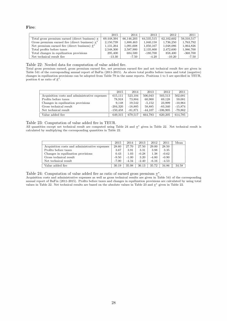
Fire:

2015 2014 2013 2012 2011Total gross premium earned (direct business) π 69,448,394 66,146,203 64,535,515 62,102,602 59,310,517Gross premium earned fire (direct business) π∗ 2,150,739 1,888,463 1,840,158 1,736,250 1,763,792Net premium earned fire (direct business) π∗ 1,131,264 1,091,608 1,050,167 1,048,086 1,064,826Total profits before taxes 2,548,300 2,587,900 2,135,800 2,472,600 1,986,700Total changes in equilization provisions 295,400 684,500 -180,700 858,400 -368,700Net technical result fire -13.30 -7.50 -4.20 -10.20 -7.50

Table 22: Needed data for computation of value added fire.Total gross premium earned, gross premium earned fire, net premium earned fire and net technical result fire are given inTable 541 of the corresponding annual report of BaFin (2011-2015). As above total profits before taxes and total (negative)changes in equilization provisions can be adopted from Table 79 in the same reports. Positions 1 to 5 are specified in TEUR,position 6 as ratio of π∗.

2015 2014 2013 2012 2011Acquisition costs and administrative expenses 615,111 523,104 506,043 503,513 502,681Profits before taxes 78,918 73,884 60,900 69,128 59,081Changes in equilization provisions 9,148 19,542 -5,152 23,999 -10,964Gross technical result -204,320 -18,885 58,885 -83,340 -15,874Net technical result -150,458 -81,871 -44,107 -106,905 -79,862Value added fire 649,315 679,517 664,783 620,205 614,785

Table 23: Computation of value added fire in TEUR.All quantities except net technical result are computed using Table 24 and π∗ given in Table 22. Net technical result iscalculated by multiplying the corresponding quantities in Table 22.

2015 2014 2013 2012 2011 MeanAcquisition costs and administrative expenses 28.60 27.70 27.50 29.00 28.50Profits before taxes 3.67 3.91 3.31 3.98 3.35Changes in equilization provisions 0.43 1.03 -0.28 1.38 -0.62Gross technical result -9.50 -1.00 3.20 -4.80 -0.90Net technical result -7.00 -4.34 -2.40 -6.16 -4.53Value added fire 30.19 35.98 36.13 35.72 34.86 34.58

Table 24: Computation of value added fire as ratio of earned gross premium π∗.Acquisition costs and administrative expenses as well as gross technical results are given in Table 541 of the correspondingannual report of BaFin (2011-2015). Profits before taxes and changes in equilization provisions are calculated by using totalvalues in Table 22. Net technical results are based on the absolute values in Table 23 and π∗ given in Table 22.

28

Household:

2015 2014 2013 2012 2011Total gross premium earned (direct business) π 69,448,394 66,146,203 64,535,515 62,102,602 59,310,517Gross premium earned househ. (direct business) π∗ 2,814,327 2,742,306 2,683,368 2,622,915 2,578,722Net premium earned househ. (direct business) π∗ 2,426,927 2,370,466 2,434,656 2,375,543 2,330,813Total profits before taxes 2,548,300 2,587,900 2,135,800 2,472,600 1,986,700Total changes in equilization provisions 295,400 684,500 -180,700 858,400 -368,700Net technical result household 15.30 12.30 14.40 14.70 16.30

Table 25: Needed data for computation of value added household.Total gross premium earned, gross premium earned household, net premium earned household and net technical resulthousehold are given in Table 541 of the corresponding annual report of BaFin (2011-2015). As above total profits beforetaxes and total (negative) changes in equilization provisions can be adopted from Table 79 in the same reports. Positions 1to 5 are specified in TEUR, position 6 as ratio of π∗.

2015 2014 2013 2012 2011Acquisition costs and administrative expenses 982,200 959,807 936,495 925,889 902,553Profits before taxes 103,267 107,290 88,806 104,431 86,378Changes in equilization provisions 11,971 28,378 -7,513 36,255 -16,030Gross technical result 484,064 394,892 402,505 445,896 477,064Net technical result 371,320 291,567 350,590 349,205 379,923Value added household 1,210,183 1,198,800 1,069,703 1,163265 1,070,042

Table 26: Computation of value added household in TEUR.All quantities except net technical result are computed using Table 27 and π∗ given in Table 25. Net technical result iscalculated by multiplying the corresponding quantities in Table 25.

2015 2014 2013 2012 2011 MeanAcquisition costs and administrative expenses 34.90 35.00 34.90 35.30 35.00Profits before taxes 3.67 3.91 3.31 3.98 3.35Changes in equilization provisions 0.43 1.03 -0.28 1.38 -0.62Gross technical result 17.20 14.40 15.00 17.00 18.50Net technical result 13.19 10.63 13.07 13.31 14.73Value added household 43.00 43.72 39.86 44.35 41.50 42.49

Table 27: Computation of value added household as ratio of earned gross premium π∗.Acquisition costs and administrative expenses as well as gross technical results are given in Table 541 of the correspondingannual report of BaFin (2011-2015). Profits before taxes and changes in equilization provisions are calculated by using totalvalues in Table 25. Net technical results are based on the absolute values in Table 26 and π∗ given in Table 25.

29

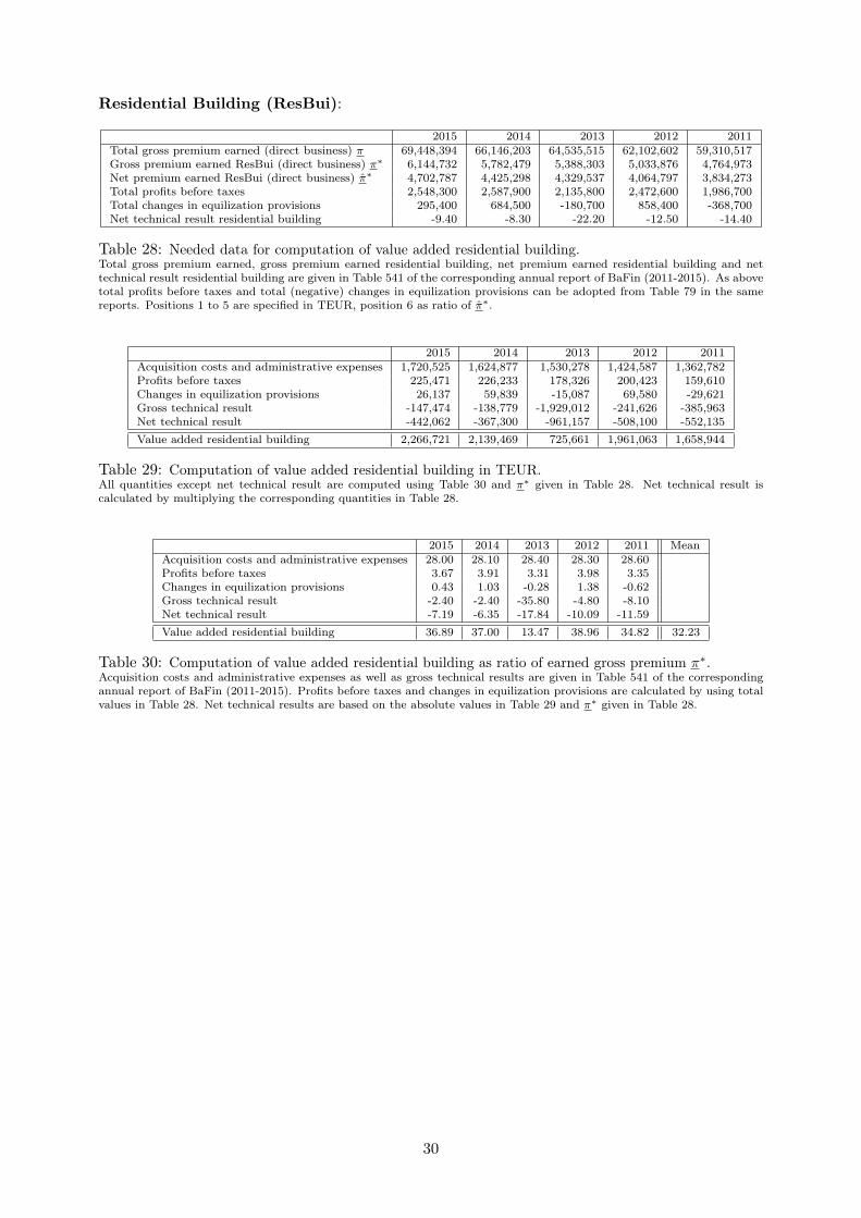
Residential Building (ResBui):

2015 2014 2013 2012 2011Total gross premium earned (direct business) π 69,448,394 66,146,203 64,535,515 62,102,602 59,310,517Gross premium earned ResBui (direct business) π∗ 6,144,732 5,782,479 5,388,303 5,033,876 4,764,973Net premium earned ResBui (direct business) π∗ 4,702,787 4,425,298 4,329,537 4,064,797 3,834,273Total profits before taxes 2,548,300 2,587,900 2,135,800 2,472,600 1,986,700Total changes in equilization provisions 295,400 684,500 -180,700 858,400 -368,700Net technical result residential building -9.40 -8.30 -22.20 -12.50 -14.40

Table 28: Needed data for computation of value added residential building.Total gross premium earned, gross premium earned residential building, net premium earned residential building and nettechnical result residential building are given in Table 541 of the corresponding annual report of BaFin (2011-2015). As abovetotal profits before taxes and total (negative) changes in equilization provisions can be adopted from Table 79 in the samereports. Positions 1 to 5 are specified in TEUR, position 6 as ratio of π∗.

2015 2014 2013 2012 2011Acquisition costs and administrative expenses 1,720,525 1,624,877 1,530,278 1,424,587 1,362,782Profits before taxes 225,471 226,233 178,326 200,423 159,610Changes in equilization provisions 26,137 59,839 -15,087 69,580 -29,621Gross technical result -147,474 -138,779 -1,929,012 -241,626 -385,963Net technical result -442,062 -367,300 -961,157 -508,100 -552,135Value added residential building 2,266,721 2,139,469 725,661 1,961,063 1,658,944

Table 29: Computation of value added residential building in TEUR.All quantities except net technical result are computed using Table 30 and π∗ given in Table 28. Net technical result iscalculated by multiplying the corresponding quantities in Table 28.

2015 2014 2013 2012 2011 MeanAcquisition costs and administrative expenses 28.00 28.10 28.40 28.30 28.60Profits before taxes 3.67 3.91 3.31 3.98 3.35Changes in equilization provisions 0.43 1.03 -0.28 1.38 -0.62Gross technical result -2.40 -2.40 -35.80 -4.80 -8.10Net technical result -7.19 -6.35 -17.84 -10.09 -11.59Value added residential building 36.89 37.00 13.47 38.96 34.82 32.23

Table 30: Computation of value added residential building as ratio of earned gross premium π∗.Acquisition costs and administrative expenses as well as gross technical results are given in Table 541 of the correspondingannual report of BaFin (2011-2015). Profits before taxes and changes in equilization provisions are calculated by using totalvalues in Table 28. Net technical results are based on the absolute values in Table 29 and π∗ given in Table 28.

30

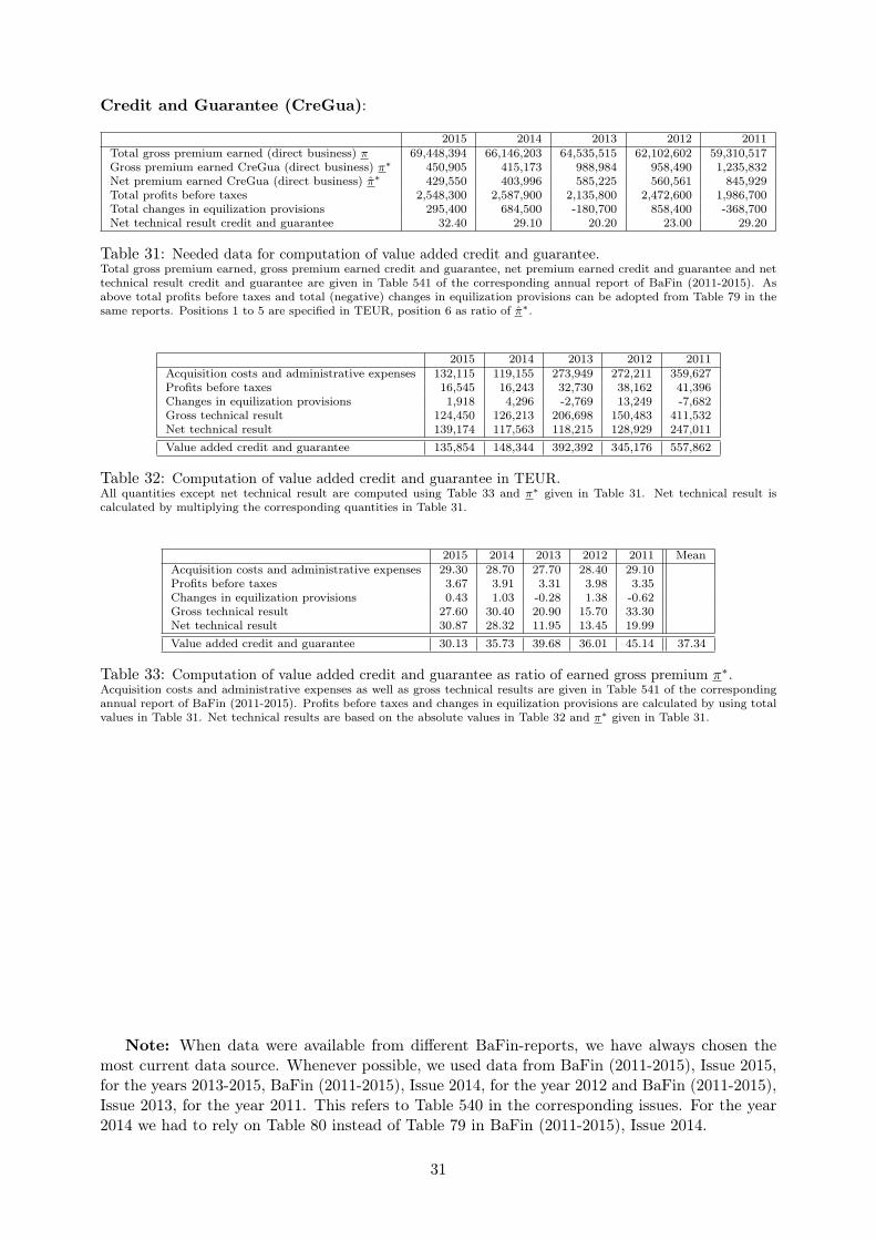
Credit and Guarantee (CreGua):

2015 2014 2013 2012 2011Total gross premium earned (direct business) π 69,448,394 66,146,203 64,535,515 62,102,602 59,310,517Gross premium earned CreGua (direct business) π∗ 450,905 415,173 988,984 958,490 1,235,832Net premium earned CreGua (direct business) π∗ 429,550 403,996 585,225 560,561 845,929Total profits before taxes 2,548,300 2,587,900 2,135,800 2,472,600 1,986,700Total changes in equilization provisions 295,400 684,500 -180,700 858,400 -368,700Net technical result credit and guarantee 32.40 29.10 20.20 23.00 29.20

Table 31: Needed data for computation of value added credit and guarantee.Total gross premium earned, gross premium earned credit and guarantee, net premium earned credit and guarantee and nettechnical result credit and guarantee are given in Table 541 of the corresponding annual report of BaFin (2011-2015). Asabove total profits before taxes and total (negative) changes in equilization provisions can be adopted from Table 79 in thesame reports. Positions 1 to 5 are specified in TEUR, position 6 as ratio of π∗.

2015 2014 2013 2012 2011Acquisition costs and administrative expenses 132,115 119,155 273,949 272,211 359,627Profits before taxes 16,545 16,243 32,730 38,162 41,396Changes in equilization provisions 1,918 4,296 -2,769 13,249 -7,682Gross technical result 124,450 126,213 206,698 150,483 411,532Net technical result 139,174 117,563 118,215 128,929 247,011Value added credit and guarantee 135,854 148,344 392,392 345,176 557,862

Table 32: Computation of value added credit and guarantee in TEUR.All quantities except net technical result are computed using Table 33 and π∗ given in Table 31. Net technical result iscalculated by multiplying the corresponding quantities in Table 31.

2015 2014 2013 2012 2011 MeanAcquisition costs and administrative expenses 29.30 28.70 27.70 28.40 29.10Profits before taxes 3.67 3.91 3.31 3.98 3.35Changes in equilization provisions 0.43 1.03 -0.28 1.38 -0.62Gross technical result 27.60 30.40 20.90 15.70 33.30Net technical result 30.87 28.32 11.95 13.45 19.99Value added credit and guarantee 30.13 35.73 39.68 36.01 45.14 37.34

Table 33: Computation of value added credit and guarantee as ratio of earned gross premium π∗.Acquisition costs and administrative expenses as well as gross technical results are given in Table 541 of the correspondingannual report of BaFin (2011-2015). Profits before taxes and changes in equilization provisions are calculated by using totalvalues in Table 31. Net technical results are based on the absolute values in Table 32 and π∗ given in Table 31.

Note: When data were available from different BaFin-reports, we have always chosen themost current data source. Whenever possible, we used data from BaFin (2011-2015), Issue 2015,for the years 2013-2015, BaFin (2011-2015), Issue 2014, for the year 2012 and BaFin (2011-2015),Issue 2013, for the year 2011. This refers to Table 540 in the corresponding issues. For the year2014 we had to rely on Table 80 instead of Table 79 in BaFin (2011-2015), Issue 2014.

31

References

Artzner, Philippe, Freddy Delbaen, Jean-Marc Eber & David Heath (1999), ‘Coherent Measuresof Risk’, Mathematical Finance, 9(3), 203–228.

Asmussen, Søren & Hansjörg Albrecher (2010), Ruin Probabilities, 2 edn, World Scientific.

BaFin, Bundesanstalt für Finanzdienstleistungsaufsicht (2011-2015), ‘Statistik der BaFin -Erstversicherungsunternehmen’.

BMJV, Bundesministerium der Justiz und für Verbraucherschutz (2017), ‘Insur-ance tax act’, https://www.gesetze-im-internet.de/englisch_versstg/englisch_versstg.html. [Online; accessed 04-April-2017].

Bundesfinanzministerium (2016), ‘Kassenmäßige Steuereinnahmen nach Steuerarten in denKalenderjahren 2010 - 2015’.

Christiansen, Marcus C. & Andreas Niemeyer (2014), ‘Fundamental Definition of the SolvencyCapital Requirement in Solvency II’, ASTIN Bulletin 44(3), 501–533.

European Commision (2017), VAT Rates Applied in the Member States of the European Union.

European Commission (2009), ‘Directive 2009/138/EC of the European Parliament and of theCouncil of 25 November 2009 on the taking-up and pursuit of the business of insurance andreinsurance (Solvency II)’. No. (64).

Föllmer, Hans & Alexander Schied (2011), Stochastic Finance - An Introduction in Discrete Time,3rd extended edn, Walter de Gruyter & Co., Berlin.

Föllmer, Hans & Stefan Weber (2015), ‘The Axiomatic Approach to Risk Measurement for CapitalDetermination’, Annual Review of Financial Economics, 7.

Holzheu, Thomas (1997), Die Belastung von Versicherungsdienstleistungen mit Verkehrsteuern,Verlag Versicherungswirtschaft GmbH Karlsruhe.

Holzheu, Thomas (2000), Die Einbeziehung der Schaden-/Unfallversicherung in das Umsatz-steuersystem, Verlag Versicherungswirtschaft GmbH Karlsruhe.

Insurance Europe (2016), Indirect taxation on insurance contracts in Europe.

Schmidt, Klaus D. (2009), Versicherungsmathematik, 3 edn, Springer.

Schrinner, Axel, ed. (1997), Versicherungsteuer als Standortproblem, Vol. 352, Institut für Fi-nanzen und Steuern, Bonn.

sigma (2012), Insuring ever-evolving commercial risks, Study 5, Swiss Re.

Straubhaar, Thomas (2006), Auswirkungen einer Erhöhung der Versicherungsteuer auf diedeutsche Wirtschaft, die Verbraucher, die öffentlichen Haushalte und den Versicherungs-standort Deutschland, Technical report, Hamburgisches WeltWirtschaftsInstitut.

Weber, Stefan (2017), Solvency II, or How to Sweep the Downside Risk Under the Carpet.Submitted.

32

https://www.gesetze-im-internet.de/englisch_versstg/englisch_versstg.html

https://www.gesetze-im-internet.de/englisch_versstg/englisch_versstg.html

The Impact of Insurance Premium Taxation - uni … · The Impact of Insurance Premium Taxation ......

Documents

Transcript of The Impact of Insurance Premium Taxation - uni … · The Impact of Insurance Premium Taxation ......