WPE 068

Yose Rizal Damuri Ari A. Perdana

May 2003

Economics Working Paper Series http://www.csis.or.id/papers/wpe068

The Impact of Fiscal Policy on Income Distribution and Poverty: A Computable

General Equilibrium Approach for Indonesia

CSIS WORKING PAPER SERIES

© 2004 Centre for Strategic and International Studies, Jakarta

The CSIS Working Paper Series is a means by which members of the Centre for Strategic andInternational Studies (CSIS) research community can quickly disseminate their research findings andencourage exchanges of ideas. The author(s) welcome comments on the present form of this WorkingPaper. The views expressed here are those of the author(s) and should not be attributed to CSIS Jakarta.

The Impact of Fiscal Policy on Income Distribution and Poverty: A Computable General Equilibrium Approach for Indonesia Yose Rizal Damuri Ari A. Perdana CSIS Working Paper Series WPE 068 May 2003

ABSTRACT The paper seeks to quantitatively measure the impact of fiscal policy on income distribution

and poverty in Indonesia using WAYANG, the CGE model for Indonesian economy. We find

that scenarios for fiscal expansion significantly influence income distribution and poverty.

Fiscal expansion mainly benefits urban households and non-labour rural households –

basically, the wealthiest segments of the society. We have are several explanations. First,

factors of production owned by these segments allowed them to reap the most benefits from

fiscal expansions. Second, these households are least affected by price increases due to their

consumption structure. Finally, we find that, in real terms, the Indonesia’s taxation system

burdens poorer households more than richer ones.

Keywords: Indonesia, income distribution, poverty, economic modelling, fiscal policy

Yose Rizal Damuri yose_rizal@csis.or.id Department of Economics CSIS Jakarta

Ari A. Perdanaari_perdana@csis.or.id

Department of EconomicsCSIS Jakarta

1. INTRODUCTION The Indonesian economic crisis that began in 1997 has been accompanied by widespread social distress in the country. A fall in output and incomes in these countries has been invariably accompanied by massive job losses as bankruptcies and cutbacks in production have multiplied. This has led to a sharp rise in open unemployment and underemployment. As the result, increasing number of people living below the poverty line and the deteriorating income distribution has been the concern of most. Unfortunately several studies on the social impact of the crisis failed to illustrate the exact impact on poverty and income distributions. Differences in assumptions and methodology have led to different figures. On the other hand, the Social Safety Net program that was implemented by the government has been considered as failure, do to the wrong design of the program which made the fund did not reach the poor people. The failure of the Social Safety Net program does not necessarily wipe out the fact that there is still the need for a good government policy to alleviate poverty and redistribute income. While stimulating economic growth is considered a longer-term remedy, the government can directly intervene through fiscal policy instruments. However, such policy should be well-designed. It means that a policy implementation should be preceded by good cost-benefit analysis, calculating the positive as well as the adverse effect. In such case, policymakers need a tool which enables them to precisely measure the net effect of a possible fiscal policy instrument. The purpose of this study is to quantitatively measure the impact of fiscal policy on poverty alleviation and redistribution policy. We are interested in fiscal policy since it can play role as a direct intervention to poverty and income distribution. Fiscal policy can also be targeted on specific groups in the economy, which suffer most from an economic shock. In some conditions, especially during a crisis period where an economy may experience negative growth, a more immediate action is required. In such condition, there will be a need for a direct government intervention translated in fiscal policies. The study may be useful to assist policy makers having a detailed policy orientation on poverty and income distribution. It seeks to provide both theoretical and empirical justification to seek and implement the “right” policy on poverty alleviation and redistribution. The term “detailed policy orientation” here means more than a simple, theoretical or intuitive consideration of fiscal policy (Francoins and Reinert 1997). It involves an analytical commitment to the details in the household and factor level as well as a commitment to be engaged in the policy-making process. A concern in the household and factor details forces the researcher into the realms of data on income distribution among and within households or income groups. It also concerns the way in which poverty or distribution measures are implemented. The study uses the Computable General Equilibrium (CGE) approach as the tool of analysis. The CGE model will be used here is called WAYANG, a CGE model designed for Indonesia. For the purpose of this research, we should first make some amendments to the original model by incorporating the parametric distribution and headcount poverty calculation. Using the model, we run four scenarios:

1

Scenario 1 examines the effects 20% increase in government expenditure under the condition of government’s budget deficit. In this scenario the government budget is allowed to change in response to the increase in the government expenditure, without having the revenue change sufficiently to cover the increase. Implicitly, this scenario ensures that the government can make borrowing to cover the increase in expenditure.

Scenario 2 deals with a different way of tax financing to cover the increase in

government expenditure. In the second scenario, income tax rate adjusts to ensure that the government borrowing is unaffected by the increase in the expenditure. By having the income tax rate adjustment, the original deficit or surplus in the government budget will not change at all.

Scenario 3 is different in the way that income tax rate adjustment is swapped to the

adjustment of sales tax. Through this swap, effects on different types of deficit financing can be examined in more detail.

Scenario 4 is basically similar to the first one, but with fixed trade balance. By having

trade balance unchanged, there is no capital flow and foreign borrowing allowed to keep private investment unaffected. The increase of public investment pushes the interest rate to soar as no foreign borrowing take place. This in turn drives the private investment to adjust towards changing in the economy. In macroeconomic terms, the last scenario deals with a condition where private investment might be crowded out due to a shock in government expenditure and investment.

The report is outlined as follows. Section two discusses the role of fiscal policy as an instrument for povery alleviation, and the current fiscal contstraints faced by the Indonesian government. Sections three and four explains the WAYANG CGE model and the simulations. Section five presents the simulation results. We conclude the discussion in section six. 2. THE ECONOMIC CRISIS, POVERTY AND FISCAL POLICY

2.2. The Transmission

The transmission from the economic crisis – characterized by the sharp output contraction and currency depreciation, high inflation and banking system failure – to the social (more specifically, poverty and income distribution) impact of the crisis could be traced from adjustment mechanisms. Following Feridhanusetyawan (1999), there are three channels of transmission (see figure 2.1). First is the adjustment at the macro level at the output and input markets, especially labor market. The second category is the adjustment at the micro level, namely the changing patterns if household income and expenditure. Finally, there is an indirect transmission through the government expenditure, namely the provision of public social services. The first channel of transmission at the macro-level consists of the adjustment in the output and input (labor) markets. In the output market, the changing structure in the economy has moved resources from one sector and industry to another. The crisis has shifted resources from the modern, non-traded and import-dependent sectors – such as construction and capital-intensive manufacturing – to traditional, traded and export-oriented sectors

2

(agriculture, forestry, mining and labor-intensive manufacturing). In the shrinking sectors, market adjustments in the form of declining profit and real income, firm insolvency, company closing, has been more severe compared with the adjustment in the booming sectors. But the fact that not every industry or sector has been suffering from the crisis and even some sectors (such as the export-oriented manufacturing and agriculture, see Booth [1999]) have in fact benefited, has led to the complexity in assessing the social impact of the crisis. The next macro-level adjustment takes place in the labor market, characterized by the fall in employment, real income and labor productivity. As a result of the flexible labor market in the naturally labor surplus economy, the increases in unemployment and underemployment rates have been relatively smaller than previously expected. But, on the other hand, the decrease in the real wage has been dramatic. Consistent with the changing structure of the economy in general, labor has moved from the formal to informal sectors, from modern to traditional sectors, and from urban to rural areas (see Feridhanusetyawan [1999], Manning [2000]). The second channel of transmission is at the micro level, takes from in the changing patterns of household income expenditure. Sharp reduction in real income has forced people to work for relatively less income, to consume their savings or to sell their assets to cope with increasing expenditure. The increase in prices has been three or four times larger than the increase in nominal wages, such that the purchasing power of the family could decline by around a half. On the expenditure side, the doubling of prices, especially food prices, has forced people to reduce and substitute their spending on secondary and tertiary needs for basic needs. For low income families, for whom food consumption accounts for most of their expenditures, the sharp increase in food prices have significantly reduces their purchasing power, lowered their food consumption, and even led to starvation in some cases. The third channel links the economic collapse and social problems through direct government expenditure. The government budgetary constraints during the crisis also led to smaller public spending for education, health and other services, as well as reducing the ability of government to maintain subsidies for fuel, electricity or basic food. Combined with the lack of capacity within the government in dealing with the crisis, the limited government budget has led to ineffective social safety net program.

3

Figure 2.1 Transmission from Economic Crisis to Poverty and Distributional Problem

FallingGovernmentRevenue

RupiahDepreciation

HighInflation

FallingOutput andEmployment

Labor Market Adjustments:•Unemployment andunderemployment (smallincrease)•Reduction in real wage andproductivity (large)

Adjustment in Household (HH) Income andExpenditure

Income:•Work more for lesssalary•Selling assets•Forcing family membersto work

Expenditure:•Sharp reduction inpurchasing power•Less savings ordissavings•Lower quality andquantity of consumptionesp. food

•Lower quality and quantity ofwelfare infrastructures (health,education, social services)•Unavailability of adequate socialsafety net

•Increase in poverty•Changes in income distribution

2.3. Poverty Figures since the Crisis

The official poverty figure is the one published by the Central Board of Statistics (BPS). The poverty rate is calculated based on the National Socio-Economic Survery (SUSENAS). Table 2.1 presents the official poverty lines, headcount poverty rates and the number of people living below the poverty line. According to the official BPS statistics, the crisis has increased the number of people living below poverty line from 34.5 million (17.7% of total population) in 1996 to 49.5 million (24.2%) in 1998. Poverty figure in 1996 was used as the benchmark since there is an absence of survey or estimation on poverty in 1997, when the crisis began. However, some opinions argued that the BPS calculation on poverty rate and incident in 1998 has been overestimated. Several studies has come up with lower numbers of the 1998 poverty rate, i.e. 14.1% (World Bank 1999), 11% (Frankenberg et al. 1999), or 14.4% (Poppele et al. 1999). Small progress in the economy, especially lower inflation and return-to-positive GDP growth has reduced the poverty incidents in the subsequent years. In 1999, BPS calculated that poverty incident declined to 37.5 million (18.2% of total population). Poverty figures in the subsequent years are estimated based on SUSENAS Core data, excluding two troubled provinces of Aceh and Maluku. This explains why poor population declined to 37.3 million in 2001, but the poverty rate is higher, 18.9%. Poverty incident continued to decline, although not much, in 2001.

4

Table 2.1 Estimates of the headcount poverty rate Poverty line (Rp) Headcount poverty rate (%) Poor population (million) Year Urban Rural Urban Rural Total Urban Rural Total1996 * 38,246 27,413 13.6 19.9 17.7 9.6 24.9 34.51998–December * 96,959 72,780 21.9 25.7 24.2 17.6 31.9 49.51999–December * 89,845 69,420 15.1 20.2 18.2 12.4 25.1 37.52000 ** 91,632 73,648 14.6 22.1 18.9 12.1 25.2 37.32001 ** 100,011 80,832 9.8 24.9 18.4 8.5 28.6 37.1

Source: BPS (various years) Notes: * Based on SUSENAS full data, East Timor included ** Estimation based on SUSENAS Core data, East Timor, Aceh and Maluku exclued Table 1.1 also suggests that in terms of increase in poverty, the crisis seems to be more an urban, rather than rural, phenomenon. This is illustrated by the increase in urban poverty by 88% from 1996-98, compared with ‘only’ 30% in the rural areas. Conversely, urban poverty also reduced faster (30%) than those in the rural areas (21%) following a relative improvement on the economic situation from 1998-99. However, the absolute number of rural poor is still higher than those in the urban areas in all years. This means that in absolute term, the level of deprivation is still higher in rural areas. The sectoral analysis of poverty incidence is illustrated by table 2.2. The table presented the sectoral changes on headcount poverty and the contribution to total poor between February 1996 and 1999. During the crisis, all sectors have indicated increase in the poverty incidence. In absolute term, the agriculture sector had the highest poverty incidence before and after the crisis. It is also consistently has the highest share of poor people of total population. Pradhan et al. (2000:20) argued that this finding implies two things First, people in agriculture sector have always been the poorest among the other sectors. The poverty incidence is still high after the crisis, despite not being hit as hard as the modern sectors. However, this argument seemed to be rather weak. In fact, not all agriculture people or regions are poor (or being the poorest among the other regions or sectors). Second, agriculture sector is also the largest in terms of employment. Therefore, although the crisis seemed to hit the modern sectors more, the absolute poverty in agriculture sector remained to be the highest. However, after the crisis the poor share of agriculture sector had declined. The declining trend of the poor share of total population had also happened in the mining and quarrying sector. On the other hand, relatively modern sectors had shown higher contribution of poor people after the crisis. Finance, leasing and insurance had experienced the highest relative increase in poverty incidence, as well as the contribution of the poor. This may be an illustration of the financial nature of the crisis.

5

Table 2.2. Sectoral Headcount Poverty and Contribution to Total Poor

Feb ‘96 Feb ‘99 Sectors Sectoral

headcount poverty

Share of sectoral poverty

Sectoral headcount poverty

Share of sectoral poverty

Changes in percentage point

Agriculture 26.29 68.54 39.69 58.38 13.40Other 13.29 0.10 32.00 0.27 18.71Mining and quarrying 15.34 1.01 29.81 1.00 14.47Construction 14.04 5.42 28.97 5.52 14.93Transport and communication 8.85 3.32 24.02 5.58 15.17Manufacturing industry 10.69 5.71 22.92 7.71 12.23Trade, hotel, restaurant 7.96 8.10 17.63 11.13 9.67Receiving transfer 6.58 1.86 15.57 2.65 8.99Electricity, gas, water 6.10 0.16 14.18 0.17 8.08Civil, social, private services 5.73 5.72 13.13 7.36 7.40Finance, insurance, leasing 1.24 0.06 5.23 0.23 3.99Total 9.75 100.00 16.27 100.00 6.52

Source: Pradhan et al. (2000)

2.4. Policy Response: the Social Safety Net failure

The role of the social safety net is crucial during the economic crisis to provide some protection for those who have to suffer from painful economic adjustments. Unfortunately, the social safety net in Indonesia, which was implemented between 1998-99 has not been effective. The implementation of the social safety net has not only been late, but also been in disarrays and full of controversy. However, to be fair, the failure of the Social Safety Net (SSN) programs was perhaps not too surprising. The worsening process of the crisis has been such that there was no warning system could be developed. Another reason was the lack of capacity within the bureaucracy in dealing with the program. The bureaucracy was not only demoralized during the rapid process of economic collapse and political turmoil, but also lacked the experience in designing and implementing the program. The problem was also complicated when the issues were politicized during the year of political turbulence in 1998. Three months after the announcement of this SSN program, there were widespread criticisms that the program was a total failure. It was reported in various media that the program did not work nor reach the poor, and even the money was corrupted. In fact the World Bank had to delay the disbursement if the loan to Indonesia, partly due to some concern that the SSN fund was not properly used. Early 1999, The National Planning Board (BAPPENAS) admitted that the disbursement of the SSN fund had been very slow, and that the program had not run smoothly. It was also reported that only around 30-40% of the fund that was actually used.

2.5. The Role of Fiscal Policy In Poverty Alleviation

2.5.1. Transmission Mechanism

This study aims to measure the net impact of different schemes of fiscal policy on the poverty incidence and income distribution in Indonesia. A fiscal scheme is any combination of fiscal instruments on the (government) revenue and expenditure. We underline the term “net impact” since each fiscal instrument implies some adverse effects to the economy, which may lessen the effectiveness of its role. In the economic jargon, the adverse effect is more familiar

6

as “efficiency cost”. However, while poverty alleviation and redistribution policies inevitably involves efficiency cost, this consequence by itself establishes no conclusive case against such policies. It merely tells us that (1) any given distributional change should be accomplished at the least efficiency cost, and (2) a need exists for balancing conflicting equity and efficiency objectives. An optimally conducted policy must allow for both concerns. An illustration of the role of different fiscal instruments and their efficiency costs is summarized in figure 2.2.

Figure 2.2.Transmission Mechanism: The Effect of Fiscal Instruments on Poverty and Income Distribution

GovernmentBudget

Adjustment in Household (HH) Income and Expenditure

Development and infrastructurespending, especially on welfareinfrastructures

•Poverty•Income distribution

Transfer to HH Commodity subsidies

Income adjustment Price adjustment

Externalborrowings

Income tax Productiontax

Work-leisure preferenceswitch; may result in smallertax revenue

Slower growth; may resultin the adjustment in thelabor market

Pressure forinflation

Areas of fiscal policies

Transmission mechanism

Possible adverse effects

Beyond the scope of the study

Sales tax

On the expenditure side, poverty alleviation and income redistribution are implemented most directly by three instruments by which the government could allocate budget. The first one is direct or personal subsidy, targeted on the low-income households. The second one is price subsidy, which is a subsidy allocated to commodities which are used chiefly by the low-income households, or specifically named as basic commodities. Due to the limitation of the model, we will only focus on these two areas of expenditure on this research. However, there is a third area of expenditure, which is the direct government spending on public services and infrastructures, especially on welfare, health and education, which particularly benefit low-income households. On the revenue side, financing can be obtained either domestically or from external funding. From the domestic side, we will be limiting our attention on income and commodity taxes. External funding can be in various forms, but will be limited on external (public) borrowings. In choosing among alternative policy instruments, allowance must be made for resulting deadweight losses or efficiency cost, i.e., costs which arise as consumer or producer choice are interfered with. A direct subsidy has the advantage that it does not interfere with

7

particular consumption or production choices. It also offers a more accurate result on improving the income distribution among households. However, this mechanism also requires some costs in the implementation. Firstly, there is an efficiency cost, since the choice between work and leisure will be distorted. There are also costs of targeting the “poor”, including the administrative cost (Subbarao et al 1999), social cost and political economy cost (Gelbach and Pritchett 1995, 1997).1 In contrast, a commodity-specific subsidy requires lower administrative cost – since it does not require household targeting effort – and no work-leisure distortion. The disadvantage is that it implies distortions in the relative price between commodities. Similar to direct subsidy, income tax implies less market distortions since it does not affect the relative prices and the production or consumption choices. But it also implies efficiency cost as it could switch the work-leisure preference of an individual subject to being taxed. In some cases, a higher income tax might reduce the overall individual working time. As the result, the tax revenue would be smaller, means lower available funding for subsidies. Taxes could also be applied on commodities which are consumed largely by high-income consumers, or – in some cases – are relatively capital-intensive. The taxes can take form of production or consumption (sales) tax, with each has specific adverse microeconomic and macroeconomic (economywide) effects. At the micro level, these taxes create relative price distortions, the impact similar to commodity subsidies. At the macro level, both create inflationary effect since it increase the prices of the taxed commodities. Furthermore, production taxes create disincentive for producer and could result in lower production and slower economic growth. A slower economic growth will imply some adjustment in the labor market, a process similar to the discussion in previous section, which in the end affect the household income and expenditure. Meanwhile, unlike the domestic taxes, external borrowings do not have direct microeconomic effect. The adjustment on domestic economy takes place only through macroeconomic variables. As a component of foreign assets, external borrowings create expansionary effect on the domestic money supply, which is a pressure for domestic inflation. This in turn creates a lower household real income and expenditure, although the result may not be clear and could be prevented by sterilization policy.

2.5.2. The Fiscal Policy Constraint

Deteriorating economic fundamentals and prolonging political uncertainty have made the Indonesian government facing a serious budgetary problem. As outlined by the IMF Letter of Intent (LoI), the government must gradually reduce its budget deficit. The government budget from 2000 to 2003 is presented in table 2.3. From the mentioned table, the government targets the budget deficit at 1.8% of GDP in 2003. This is a revised figure due to the Bali blast incident, from previosly 1.6%. The government also expects to have zero deficit in 2004. However, given the fluctuation of Rupiah, slower-than-expected economic growth and the inflationary pressure which forced the interest rate to remain high, the government is facing a heavy task in managing its budget deficit. Financing the deficit is another difficult task, as the progress of privatization and asset sales, by which the government expects the revenue, is

1 Without undermining the significance of such costs, however, this issue will not be addressed on this research.

8

somewhat slow. Meanwhile, starting 2004 the government will also face a fiscal time bomb, the domestic interest payment burden. To anticipate the exploding deficit, the government prepared to undertake several actions. The planned actions include squeezing development expenditure, which includes spending on welfare infrastructures, and reducing the allocation for subsidies. As the consequences, the most serious impact in the medium and longer run is the deterioration of public services in health and education. The provision of public services in education and heath for the poor has declined, and the long run adverse impact on poverty is very serious. The impact of the crisis on education and health in terms of quantity has been less severe than expected, but the impact on the quality in very serious. The low quality of health and education services is taking its toll, and the impact in the longer terms would be enormous. This situation clearly suggests that the government is now having a heavy fiscal policy constrain. However, the prolonging crisis also means that the economic performance still does favor the poor and the relatively worse-off. Direct intervention on the poverty alleviation and income distribution improvement programs are still required through fiscal instruments. Therefore, a good detailed calculation on the cost and benefit of such programs is then needed.

Table 2.3. Indonesia: Government Budget (as % to GDP), 2000-03

2000 2001 2002 2003 A. TOTAL REVENUE 15.1 19.3 17.9 17.3 I. Tax revenue 10.7 12.9 13.0 13.1 II. Non-tax revenue 4.4 6.5 4.9 4.2 B. GOVERNMENT EXPENDITURES 20.1 23.2 20.4 19.1 I. Central Government Expenditure 15.8 17.8 14.6 13.1

1. Routine Expenditures 3.2 14.9 11.5 9.7 2. Development & net lending 4.3 2.9 3.1 3.4

II. Balanced Fund 0.0 5.5 5.6 5.8 D. BUDGET DEFICIT -5.0 -3.8 -2.5 -1.8 E. FINANCING 5.0 3.8 2.5 1.8 I. Domestic Financing 2.4 2.5 1.4 1.2 II. Foreign financing 2.5 1.4 1.4 0.6 Source: Ministry of Finance, Financial Notes, various years

9

3. WAYANG: A CGE MODEL FOR THE INDONESIAN ECONOMY2

3.1. The WAYANG Model

WAYANG is a single country CGE model of Indonesian economy designed for comparative-static analysis of particular economic policy.3 The theoretical structure of WAYANG model is built closely on that of ORANI, a single region model of Australia (Dixon et. al 1982). It belongs to the class of general equilibrium model, which is linear in proportional changes. This model is originally developed by Warr (1998) and documented and developed further by Witwerr (1999) and others under the ACIAR Indonesia Research Project. Most of the CGE models, including WAYANG model, which is used in this study, come under the category of comparative static model. It means the analysis produces the change between equillibria given a change in economy. This type of model is particularly useful in analyzing long run effect of a certain proposed economic policy. CGE models can also be categorized as a domestic or multi region one. Multi regions models tried to capture the relation between economies, usually represented as a particular country. The domestic or single country region put more concern on a single country’s economic activities. WAYANG model falls into this classification, whereas the model also provides regional analysis within the Indonesian economy. Table 3.1 describes the disaggregation of institutions, factors of production, activities and household in details. In general, the model differentiates household, government, industry and the rest of the world as different institutions. There are ten different groups of household in the economy based on the dominant source of income factors. These households control factors of production. The factors of production can be categorised into five primary factors and one specific factor of production. The model distinguishes 65 groups of private industries, which use these factors in their activities. The industries provide 65 different commodities, of which five are considered as margin commodities. Other institutions appear in the model are the government and the rest of the world. The extension of WAYANG model is constructed into regional disaggregation. However, this essay only put concern on the basic of the model.

2 Most of this chapter is adopted from Wittwer (1999), except the section on the amendment to the model. 3 For complete description of WAYANG, visit the model website on http://www.adelaide.edu.au/cies/indlist.htm.

10

Table 3.1. Sets and Elements of WAYANG Model

Sets Elements Disaggregation

Institutions private intermediate, private investment, household, government, rest of the world

Household Rural landless, small, medium, large farmer, poor non-agr. labour, non labour, rich non-agr labour

Urban poor labour, non-labour, rich labour Industries Agriculture Paddy, Maize, CassOroot, GroundNut,

SoyOtBeans, VegFruit, OFooFibCr, RubberRaw, SugarCane, Coconut, OilPalm, Tabacco, Coffee, Tea, OthAgric

Non-agriculture

LivestoProd, Wood, ForestHunt, SeaProduct, agricservice, Coal, CrudeOil, NatGas_GThr, MetalOreMini, Quarrying, Meat, PreservFood, Copra, AnmVgOil, Rice, WheatProd, SugarConfect, ProcessFood, AnimalFeeds, AlcohTabac, NonAlcBvrgs, Yarn_Kapok, Textile, KnittMills, Clothing, CarpetRope, Leather, ManuWoodProd, ManuPaperPro, ManuChemical, Fert, Pest, PetrlRefPr, LiqNatGas, ManuRubbPlas, ManuNonmetal, ManuIronStee, ManuNFBM, ManuMetal, ConstrEquip, Machinery, CommunEquip, ManuElectric, TransRepair, OthManu, ElecGasWat, Construc, Trade, RestHotel, RoadRailTrav, SeaAirTrav, SrvcToTrans, Cmunication, BankInsur, BusiReales, GovDef, Othserv

Factors of Production

Non-agriculture skilled and unskilled labour, variable and fixed capital

Agriculture unskilled labour, fertiliser, variable capital,land

3.2. Distributional Aspects of the Model

The distinguished feature of WAYANG model is the capability of the model to estimate the distribution impact of economic policy. This feature comes from the mechanism that channeled the value added from production process into the income of different types of households and other institutions through the return to factors of production. Figure 3.4 shows the linkages between production sectors in the economy into the income of households. The relation is provided by the ownership of factors of production. Demands of commodities from different households and institutions in the economy, determined the level of output produced by the production sectors. Households pay the particular amount of money regarding their consumption and demand. It generates the demand for labor of different types mobile and fixed capital, as well as land, which belong to households and other economic institutions. The primary income distribution is, on the other hand, determined by the value added streams from the production sectors to different types of factors of production. Each factor receipt

11

different rate of return; wages is going to labor, rents is going to land and profit to capital. The distribution of income depends on the ownership of different factors of production for each household. Household that abundantly own unskilled labor receipt more unskilled labor wages, which make it has different income to other household that provide more skilled labor. In translating the factorial distribution into income distribution, the classification of households based on the factor of production ownership is the crucial factor.

Figure 3.4. Sectoral Linkages in the WAYANG Model

Production Sectors

Households Factors of Production

WAYANG model categorize household in the Indonesian economy mainly based on the resource endowment and location of a particular household. This classification, following the one used in the Indonesian Social Accounting Matrix (SAM). The name of each household group explains the main source of income for household in the group. characteristics determine how the effects of shocks in the simulation distribute among different types of household.

3.3. Database

WAYANG database is arranged in the form of Input-Output database, which is categorised into various economic agents and components. Database used in the WAYANG model is based heavily on the 1995 social accounting matrix (SAM 95) and 1995 input-output tables produced by BPS. Other supplementary data sources provide additional information used in the construction of specific tables such as for fiscal extension or import tax data.

12

Table 3.2. Households Population and Expenditure Population Consumption

Expenditure Household Categories Total

(million) Share (%)

Total (Rp. Bill)

Share (%)

Per capita Expenditure

HH1 Landless 20.79 10.68 12,407 3.45 596.66 HH2 Small Cultivator ( < 0.5 ha.) 32.99 16.94 29,642 8.24 898.48 HH3 Medium Cultivator (0.5 to 1 ha.) 13.80 7.08 15,256 4.24 1,105.82 HH4 Large Cultivator ( > 1 ha.) 10.70 5.49 16,401 4.56 1,533.26 HH5 Non-Agricultural labour: low income 28.70 14.74 38,084 10.58 1,326.87 HH6 Rural non-labor households 9.10 4.67 9,414 2.62 1,034.79 HH7 Non-Agricultural labour: high income 15.27 7.84 57,486 15.98 3,765.17 HH8 Urban labour: low income 33.84 17.37 59,869 16.64 1,769.45 HH9 Urban non-labour household 10.20 5.24 16,603 4.61 1,628.17 HH10 Urban labour: high income 19.38 9.95 104,686 29.09 5,402.72

Source: BPS, Sistem Neraca Sosial Ekonomi Indonesia 1995 and WAYANG Database

In order to look at how the way of external shocks affect the various household aspects of the model, it is important to summarise the characteristics of the ten households represented in WAYANG. Table 3.2 provides this summary. The seven rural households account for 73% of total population and 61% of total consumption expenditure. The four poorest household categories, measured in terms of expenditure, are all rural. Poverty, in Indonesia as elsewhere in the developing world, is overwhelmingly a rural phenomenon. The sources of income for the various households are important for the general equilibrium properties of the model and these are summarised in Table 3.3. These characteristics determine how the effects of shocks in the simulation distribute among different types of household.

Table 3.3. Household Data Characteristics Household Categories Skilled

Labour Unskilled Labour

Land Fixed Capital

Variable Capital

HH1 Landless 1.17 45.59 27.39 7.60 3.49 HH2 Small Cultivator ( < 0.5 ha.) 5.75 24.99 48.87 12.67 1.49 HH3 Medium Cultivator (0.5 to 1 ha.) 2.59 13.40 54.72 15.65 9.41 HH4 Large Cultivator ( > 1 ha.) 3.73 7.29 57.76 16.38 9.22 HH5 Non-Agricultural labour: low income 6.16 38.07 28.78 8.56 6.71 HH6 Rural non-labor households 24.59 12.77 35.26 9.38 2.35 HH7 Non-Agricultural labour: high income 19.98 4.30 46.26 14.04 12.25 HH8 Urban labour: low income 12.26 23.28 44.26 11.97 3.99 HH9 Urban non-labour household 17.78 34.12 20.65 5.73 2.63 HH10 Urban labour: high income 23.53 1.32 55.40 14.82 4.09

Source: BPS, Sistem Neraca Sosial Ekonomi Indonesia 1995 and WAYANG Database

3.4. Amendment to the Model

Despite the advantage of WAYANG model to evaluate the distribution impacts of certain economic policies, the model, however, is not able to address poverty and income distribution

13

issues properly since they do not provide any information on intra-group distribution. This issue should be addressed appropriately to obtain a better insight on poverty, considering that the household classification is not based directly on the level of income itself. Some preliminary works has been done to the model using the mean income of every household as a basic of income distribution analysis (Damuri 2000). However, the assumptions behind this approach are obviously weak and unjustified. They involve the assumption that income is distributed evenly within each group of households. Further works are required to make analysis on income distribution more advantageous.

3.4.1. Parametric Distribution

To assess the impact on poverty through the CGE model, several approaches have been suggested and applied in some models. One method was discussed in details by Dervis et al (1982). This approach consists of assigning a parametric distribution function on income or expenditure for each group, allowing for further poverty and income distribution analysis. The flexibility and easiness of this method make this approach is commonly accepted for incorporating income distribution and poverty aspects of a CGE model. The distribution of income within each group can be represented by a frequency function characterizing distribution within group. Lognormal distribution function is widely used to present income distribution within household groups. Another alternative formula for income distribution is the Beta distribution function, which allows the distribution to be skewed to the left or to the right depend on the choice of parameters representing characteristics of each household group. Decaluwe et al (1997) has used the distribution extensively in their archetype model. The distribution can be represented in the formula below:

(1) ),,( qpmnmx

mnyIPDF−−

=

where I(x, p, q) is incomplete Beta distribution, known as:

(2) 11 )1(1),,( −− −= qp xxB

qpxI

and:

(3) dxxxqpB qp∫ −− −=1

0

11 )1(),(

Unlike lognormal distribution, which depends on the mean and variance of a population, the Beta distribution are determined by the maximum, mx and minimum value, mn within the group of population as well as the parameters p and q. These parameters influence the shape and skewness of distribution. This study will employ the Beta distribution function in order to get intra-group distribution for every household group in WAYANG model. In order to find the appropriate beta distribution for each household group several statistical parameters related to expenditure data used in WAYANG database are derived from available data. The required parameters include mean or average of the group’s expenditure, the standard

14

deviation or variance within the group and the range of expenditure for every household group. Table 3.4 summarizes characteristics of expenditure data for every group. These statistical parameters are estimated from various data sources available from Indonesian Bureau of Statistics (BPS) such as SUSENAS and SKTI. In estimating the parameters, several difficulties arise as the model’s database was compiled based on several other data available. The main obstacle deals with data outliers. As the data in each household group have a very wide range value, adjustment on several parameters are required, especially for the maximum value of every group. However, the adjustment

Table 3.4. Statistical Parameters of Group’s Expenditure Data

Consumption (Rp thousand) Households Pop. (mill) Total (bn) Mean Std.Dev Max Min

HH1 Landless 20.79 12,407 596,657 327,990 1,688,324 93,502 HH2 Small Cultivator ( < 0.5 ha.) 32.99 29,642 898,477 506,681 2,239,832 109,342 HH3 Medium Cultivator (0.5 to 1 ha.) 13.80 15,256 1,105,824 604,805 2,966,869 157,920 HH4 Large Cultivator ( > 1 ha.) 10.70 16,401 1,533,256 859,510 4,450,303 214,832 HH5 Non-Agricultural labour: low income 28.70 38,084 1,326,873 765,219 3,099,226 89,286 HH6 Rural non-labor households 9.10 9,414 1,034,786 634,148 3,301,211 114,762 HH7 Non-Agricultural labour: high income 15.27 57,486 3,765,170 2,134,480 8,700,743 264,878 HH8 Urban labour: low income 33.84 59,869 1,769,453 1,071,808 4,975,671 143,572 HH9 Urban non-labour household 10.20 16,603 1,628,174 980,593 4,599,714 156,527 HH10 Urban labour: high income 19.38 104,686 5,402,721 2,893,519 11,917,069 749,669

Source: BPS, Sistem Neraca Sosial Ekonomi Indonesia 1995, SUSENAS, SKTI and WAYANG Database The representative of probability distribution for each household appears on the appendix. These distribution are based on the particular beta distribution parameters estimated using various statistical parameters described above. The relationship between parameters p and q in the beta distribution and various statistical parameters of the expenditure data can be described using the formula below:

(4) )12)1(( −

−=

s

xxxp

(5) )12

)1(()1( −−

−=s

xxxq

while

(6) n

n

i ixmeansamplex

∑== 1:

(7) 2

1)(1var:2 ∑

=−=

n

ixixniancesamples

3.12.2. Poverty and Income Distribution Measurement

After having appropriate distribution for every household group, WAYANG model will be able to carry income distribution effect and poverty analysis of a particular economic shock. Here we use the most common approach for poverty measurement, the headcount ratio:

15

(8) nqH =

where q is the number of population living below the poverty line and n is the total population. In addition to poverty incidence measurement, this model will also be completed by an income inequality measurement. Gini coefficient is the most frequently used to asses the rate of overall income inequality:

(10) ( )∑ −+−=n

iiii FFfGR 11

where f is the frequency of population in the i th class, while F is the cumulative frequency of the particular class. The value of Gini Ratio lays between 0 and 1. 4. SIMULATION AND CLOSURE

4.1. Overview

The focus of the simulation conducted in this study is to examine the implications of various fiscal policies on the Indonesian economy, including the distributional impacts on income and poverty.4 The main feature of the simulation is a 20% across the board increase in the two major components of government expenditure, namely government consumption and investment. Another component of government expenditure, which is transfer payment, is kept constant. This study also simulates the differential impact of various financing mechanism and different macroeconomic closure on the economy. In other words, the study estimates not only the impact of general increase in expenditure but also the effect of various financing schemes and different treatments and assumptions of macroeconomic set-up. The first section of this chapter discusses the closure used in all scenarios. The second section explains the treatments of poverty and income distribution aspects of the simulation. The final part discusses specific closures related to a particular scenario.

4.2. General Model Closures for the Simulation

One important factor in conducting a simulation in a CGE model is the choice of model closures in the simulation. Like many other mathematical models with many equations, a CGE model often has fewer equations than variables. In general, the variables can be classified into endogenous and exogenous variables, depending on whether the values are determined within or outside the model. In order to obtain a unique equilibrium solution and to measure the impact of a certain simulation, the number of endogenous variables must be equal to the number of equations in the model. Therefore, a closure could be interpreted as a selection of endogenous and exogenous variables that is used or assumed in the model. In economics sense, a choice of closure provides the macroeconomic setting to conduct a certain simulation. The usual simulation conducted in a CGE model is to change the value of a certain exogenous variables, of which sometimes are called policy variables because it reflects some policy changes, and to measure the impact of the changes on the equilibrium 4 For the purpose of this study, we modified the original WAYANG CGE-model by developing additional equations and closures, and incorporating new data sets to be able to capture the impact of economic shocks, like fiscal policies, on poverty and income distribution.

16

values of endogenous variables. Therefore, a closure provides certain macroeconomic assumptions behind the simulation. In that sense, a closure could reflect at least two important macroeconomic issues. First, the closure is associated with the period of time that would be needed for the economy in the model to adjust fully as results of a particular economic shock; it may take form as a short run adjustment or a long run adjustment. Second the closure provides the assumptions needed for a particular simulation and describes various approaches to certain variables that the model could not explain in detailed. In this regard, the WAYANG model falls into a category of static and real economic model that has no detailed description of monetary and financial economic variables such as money demand and supply, interest rates and capital accumulation. In other words, the WAYANG model is a real sector model in which policy shocks affect the equilibrium values instantly. Because the model has not inter-temporal mechanism of adjustments, there is no explicit financial and monetary transmissions such that trace the movement of interest rates, exchange rates, and financial capital flows. The simulation conducted in this study is intended to examine the result of 20 percent increase in government expenditure, in the form of consumption and investment, under a static general equilibrium framework. The closures must be made to reduce the inconsistencies between the nature of single period model and multi period aspects of certain variables in the model. The closures that are used in all simulations in this study are described in Figure 4.1 Exogenously determined variables are presented by variables in rectangles, while the endogenous are those in ovals. The upper part of the diagram presents the supply side of the economy, which consists of factor inputs, such as employment, land, capital, and technical change. The demand side of the economy is illustrated in the lower part of the diagram, which describes the components of GDP like consumption, investment and trade balance. The linking arrows illustrate the direction of interdependences between variables. It is just a simplification as in the simulation the effects of a particular shock will be determined simultaneously. In the supply side, what matters in affecting individual’s income is the payment to factor of production that the individual holds. In the labor market for example, the changes in labor’s income is reflected in the changes in value of the labor input to production sectors, which can be decomposed into changes in employment and wage. The closure in this model assumes a fixed real wages, so that any shock in the economy is absorbed through changes in employment. Labors are freely moving between sectors in the economy, while the total stock of labor is fixed. The number of labor in the market will adjust according to the change in the labor demand, without affecting the level of real wages. In short, it is assumed that the labor markets are not fully employed during the period of adjustment, which commonly fit the situation of labor surplus economy in the developing countries like Indonesia. The model also assumes that other factors of production such as land and capital stocks remain unchanged, as it takes some time for those factors to be affected by the economic shock. However, as the use of capital is also affected by investment, the capital usage in a particular industry may adjust to the change in investment.

17

Figure 4.1 General Closures of The Simulation

Trade Balance

Real Devaluation

Foreign Debt

GDP = Private Consumption +

Employment Land

Investment + Government Consumption +

Public Private

Real Wages

Capital Technical Change

Rate of return In the demand side, the shocks take place in the form of 20 percent increase in government consumption and investment. These shocks will generate adjustment in the demand side, forcing GDP and variables in supply side of the economy to adjust to the changes, including the change in demand for factors of production. As labor market can adjust freely to the demand change, employment increase in the case of increasing demand without significant adjustment in real wages, which in turn leads to an increase in GDP. The change in government and public spending would also lead to a change in domestic absorptions. This simulation assumes that trade balance move freely towards deficit in response to the increase in government expenditure. By allowing the balance of trade to change, the capital flow also move freely towards deficit or surplus generated by the change in domestic absorption. Implicitly, the closure also allows foreign borrowing to take place in the economy, financing the change in investment without adjustment in the rate of return or interest rate. Here, the model assumes a fixed interest rate, and therefore a constant real private investment to restrict the inter-temporal effects of investment. In other words, private investment is not crowded out by the increase in government expenditure.

4.3. Poverty and Income Distribution Aspects

As explained in the previous section, the distribution of income across different household groups depends on types and the amounts of factors of production that a particular household owns. For example, the household group that owns skilled labor relatively more than other factors of production will receive their income mostly from the wage payment to that category of labor. Each type of factors of production has different values of value-added depends on the return to the factor and the quantity used in the economy. The difference in ownership, types, and value added of different factors of production is the main point to

18

understand the link between the adjustment of an economic shock and the distribution of income across household groups. An economic policy in a simulation affects the utilization of factors of production in either one of two ways; it changes the return to factors of production or adjusts the quantity of the factors used in the economy. The change in one of the two variables would lead to a new formation of value added to a particular factor of production. This, in turn, changes the value of value added received by household groups. An increase in demand of skilled labor as a result of a certain economic shock would lead to an increase in value of skilled labor, and in turn would make the value added obtained by household groups that owned this factor increase as well. The increase in the value of skilled labor comes from the increase in wages (price), or employment (quantity), or the combination of the two. The simulation in this study is conducted under the short run and static macroeconomic closure. As explained in the previous section, this closure assumes the rigidity of wages in all labor market, while the number of labor itself can move freely toward the economic adjustment. The change in demand of factors of production is transformed to a change in the number of labor employed in the production sector instead of adjustment in wage rates. Although the changes do not take place in wage rates, the results on distribution of income across households are similar. The change in number of employment would adjust the value added received by household groups that in turn change the distribution of income between groups. The changes in distribution of income among different groups of household serve as a basic framework in determining changes of income distribution in each group, using the method explained previously. However, since the model only has information on the value added to factors of production owned by households as a group, not individual household, there is no information available on the change of value added for the individual one. Based on the information, the change in income or expenditure variables can only be assumed to distribute equally among households within each group. In a more technical term, the simulation only affects the average of income and expenditure variables of each group, and does not affect the variance of income distribution within the group. The distributional aspect of the simulation comes from the fact that the overall distribution of income and expenditure of the entire population will change because the change of average income and expenditure varies between one group of household and another.

4.4. Simulation Scenarios

In order to have detailed examination on the effects of 20% increase in government consumption and investment, the simulation is based on four different scenarios. The first three scenarios use the general closure described above, where trade balance is floating. The different between those three scenarios is in the way the increase in government expenditure is financed. For each scenario different type of tax rate adjustment is assigned to cover the increase in government expenditure. The last scenario is a variant to the first scenario with a different treatment of trade balance. The first scenario examines the effects of 20% increase in government expenditure that is financed by an increase in government’s budget deficit. In this scenario the government budget deficit is allowed to increase sufficiently to finance the 20 percent increase in the government expenditure, without having the revenue to change to cover the increase.

19

Implicitly, this scenario ensures that the government can make borrowing to cover the increase in expenditure. The second and third scenarios deal with different ways of tax financing to cover the increase in government expenditure. In the second scenario, income tax rate adjusts to ensure that the government borrowing is unaffected by the increase in the expenditure. In other words, the budget deficit is fixed. In the third scenario, income tax rate adjustment is replaced by the adjustment of sales tax. Through these different ways of financing, the effects of different types of deficit financing can be examined in more detail. This type of scenario is widely used in many CGE simulations to demonstrate the effect of different ways in financing budget deficit. Horridge et all(1995), for example, used the similar approach in conducting their simulation on fiscal expansion in South Africa. The fourth scenario is a slight modification of the first scenario. Similar to scenario 1, it assumes that the increase in the government’s expenditure is financed through borrowing, creating higher deficit in the budget. However, this scenario assumes a fixed trade balance. By having trade balance unchanged, there is no capital flow and foreign borrowing allowed to keep private investment unaffected. The increase of public investment pushes the interest rate to soar as no foreign borrowing takes place. This in turn drives the private investment down to adjust to the changing economic condition. In macroeconomic terms, the last scenario deals with a condition where private investment might be crowded out due to a shock in government expenditure and investment. 5. RESULTS

5.1. Macroeconomic Impacts

Summary of the macroeconomic or economywide impacts of fiscal expansion under the four scenarios is presented in table 5.1. In this section we will discuss four aspects on the macroeconomic impacts: 1) the effects on Gross Domestic Product (GDP), 2) the effects on employment, 3) changes in the government budget, and 4) the household impact.

20

Table 5.1 Economy Wide Impacts of Government's Spending Expansion

Scenario Impact on 1 2 3 4Overall Economy:

Gross Domestic Product Nominal 3.53 1.06 2.61 0.84Real 1.97 0.93 0.45 0.83

GDP Deflator 1.53 0.12 2.16 0.01Employment:

Skilled 7.68 5.09 3.92 5.04Unskilled 3.93 1.54 0.55 -0.04

Return to variable capital (nominal): Non-agriculture 0 0 0 0Agriculture 2.12 -1.43 -2.82 0.71

Government Budget: Revenue (nominal) 3.12 16.31 16.4 0.1Expenditure (nominal) 18.96 18.34 18.44 14.56Budget Deficit (Rp bill) 12,142.35 -- -- 11,359.58Changes in Tax * -- 2.98 4.68 --

Household Sector: Consumption

Nominal 3.4 -1.74 0.19 0.8Real 2.07 -1.53 -3.09 0.6

Consumer Price Index 1.31 -0.21 3.38 0.2Real Rate of Return 0 0 0 31.78

Notes: All results are percentage change unless otherwise stated

* The change is percentage changes in the power of tax (1 + tax rate)

Gross Domestic Product

It is expected that the strongest effect of fiscal expansion is obtained from scenario 1 because fiscal expansion is financed by loan, which will be paid in the future, so that there is no crowding out effect trough tax increases. This reflects the static nature of the model in which the economic agent does not expect to pay back the debt through higher taxes and lower potential income in the future. However, when the budget deficit is accompanied by fixed trade balance (scenario 4), the impact of fiscal expansion on real GDP is smaller than that of scenario 1. Consistent with the closure developed for model, fixed trade balance means that the real rate of return on capital or real interest rate increases as a result of fiscal expansion. Higher interest rate leads to lower private investment and crowds out the positive effect of fiscal expansion on aggregate demand. In other words, the total positive effect of fiscal expansion on real GDP is reduced. In contrast with scenario 1, the real interest rate is kept constant by floating the balance of trade. With a fixed interest rate, any pressure to raise interest rate will be offset by the inflow of foreign capital inputs and therefore changes in trade balance. The simulation results confirm the hypothesis. An increase of government spending and investment by 20%, or 2.24% of GDP, leads to an increase of nominal GDP by around 3.3% in scenario 1, and by 0.8% in scenario 4. In real term, scenario 1 consistenlty gives the biggest impact, 1.97%, while the other scenarios only lead to a less than 1% increase of real

21

GDP. Prices also tend to be constant in scenario 4, since trade balance is fixed under the scenario. Consequently, any fiscal expansion and increase in domestic demand has to be filled by domestic supply, so there is both demand and supply expansion. Scenario 2 and 3 lead to the increase of nominal GDP by 1.06% and 2.61% respectively. Nevertheless, the increase of real GDP is higher in scenario 2 (0.93%), compared with that in under scenario 3 (0.45%), as scenario 3 leads to increase in prices by 3.3.8%. Conversely, prices decline by 0.21% in scenario 2. The reason for this is clear. The increase in sales tax has a direct impact on prices and leads to higher increase in prices compared with the results of other scenarios. On the other hand, an increase in income tax would reduce overall income and depress demands, which in turn lower inflationary pressure. The higher impact on real GDP expansion under scenario 2 implies that financing fiscal deficit through income tax has a larger effect on real GDP because the impact on prices can be minimized.

Employment

In the model, we implicitly assume that the adjustment in the labor sector is captured by changes in employment rather than in wages. Hence, our analysis regarding to the labor market only concerns on the changes in employment after the shock. The effects on employment is consistent with changes in GDP. The highest impact is obtained from scenario 1, with a 7.68% increase in employment. Scenario 2 and 4 gives relatively similar effects, increasing employment by around 5%, while scenario 3 only increase employment by less than 4%. Government Budget.

From the expenditure side, a 20 % increase in the government spending and investment leads to around 18-19% increase in total government expenditure. The difference basically arises from the transfer of payment which is assumed to be fixed. In scenarios 1 and 4, as expected, budget deficit increase by Rp11-12 trillion. That is equal to 2% to GDP. Note that despite all increases in expenditure are financed through increasing budget deficit, there is still increases in tax revenue in both scenarios. This is due to the increase in tax base, i.e. higher income gained because increased budget deficit provides stimulus to the economy. In scenarios 2 and 3, the increase of government revenue needed to finance the 18.4% on expenditure is 16%. It is interesting to note that the necessary increase in income tax rate is lower than that of the sales tax in order to finance the 20% increase in government spending and investment. Measure by the power of tax (defined by 1 + tax rate), the required increase in income tax is estimated to be 3% while that of sales tax is 4.7%. Effect on Personal Consumption

The impact of fiscal expansion on personal consumption plays a crucial role in determining poverty level because the changes in personal expenditure is used to calculate the changes in poverty level. The results of the simulation clearly show that the significant increase in personal consumption takes place in scenario 1, in which fiscal expansion is financed by budget deficit. In fact, the impact of fiscal expansion on personal consumption is negative when fiscal expansion is financed by taxes. In other case, when budget deficit is accompanied by fixed trade balance (or increase in interest rates), the impact of fiscal expansion on the increase in personal consumption is small.

22

Based on scenario 1, 20% increase in government spending and investment is expected to raise personal consumption by 3.4% in nominal term and 2.1% in real term. But based on scenario 2, when fiscal expansion is fueled by higher income tax, the impact on personal spending is estimated to be –1.74% in nominal terms and –1.55% on real terms. This is not surprising because an increase in income tax would directly reduce personal consumption. It is interesting to note that the decline in real consumption expenditure is larger when the sales tax, rather than income tax, is used to finance the budget expansion. The result of scenario 3 shows that household consumption increases by 0.19% in nominal term, but decline by 3.09% in real term, because prices (CPI) is expected to increase by 3.4%. The results confirms the notion that the change in personal consumption depends on inflation because what matters in poverty alleviation is not the changes in nominal but real expenditure. In other words, small increase in nominal personal expenditure could potentially lead to large increase in real expenditure, and rapid decline in poverty level, when inflation is low.

5.2.Output and Trade

The analysis of this section concerns on: 1) changes in sectoral output, 2) changes in industry-level oputput, 3) changes in commodity prices, and 4) the impact on the international trade.

Sectoral output

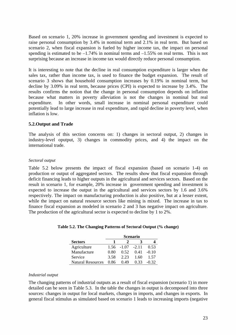
Table 5.2 below presents the impact of fiscal expansion (based on scenario 1-4) on production or output of aggregated sectors. The results show that fiscal expansion through deficit financing leads to higher outputs in the agricultural and services sectors. Based on the result in scenario 1, for example, 20% increase in government spending and investment is expected to increase the output in the agricultural and services sectors by 1.6 and 3.6% respectively. The impact on manufacturing production is also positive, but at a lesser extent, while the impact on natural resource sectors like mining is mixed. The increase in tax to finance fiscal expansion as modeled in scenario 2 and 3 has negative impact on agriculture. The production of the agricultural sector is expected to decline by 1 to 2%.

Table 5.2. The Changing Patterns of Sectoral Output (% change)

Scenario Sectors 1 2 3 4Agriculture 1.56 -1.07 -2.11 0.53Manufacture 0.80 0.52 0.41 -0.10Service 3.58 2.23 1.60 1.57Natural Resources 0.86 0.49 0.33 -0.32

Industrial output

The changing patterns of industrial outputs as a result of fiscal expansion (scenario 1) in more detailed can be seen in Table 5.3. In the table the changes in output is decomposed into three sources: changes in output for local markets, changes in imports, and changes in exports. In general fiscal stimulus as simulated based on scenario 1 leads to increasing imports (negative

23

growth of import substitution) and lower exports (negative growth of export). In other words, increasing demands in the domestic market are met by an increased in domestic supply and import, and a lower level of export. By looking at various industries, large increase in industrial output takes place in construction by 5.69%, followed machinery (2.33%), real estate (1.63%) and petroleum refinery (1.59%). Output in the natural resources and sea products industries change by only less than 1%, while textile and clothing industries expect declines in their output by 0.06% and 0.51% respectively.

Table 5.3. The Impact of Fiscal Stimulus on Industrial Output (% change)

Scenario 1: Budget Deficit Financing Sources of Change Industry

Local Market

Import Substitution

Export

Total Change

Paddy 1.43 0.00 0.00 1.43 Livestock 1.56 -0.13 -0.02 1.41 Wood 1.14 0.00 -0.02 1.12 Sea products 1.00 0.00 -0.22 0.78 Rice 1.48 -0.04 0.00 1.44 Sugar and Confectionary 1.26 -0.07 -0.09 1.10 Textile 0.81 -0.16 -0.71 -0.06 Clothing 1.04 0.00 -1.55 -0.51 Petroleum Refinery 2.18 -0.07 -0.52 1.59 Machinery 3.75 -0.88 -0.54 2.33 Electronics 2.74 -0.58 -0.88 1.28 Construction 5.69 0.00 0.00 5.69 Trade 1.77 0.00 -0.28 1.49 Real Estate 2.05 -0.34 -0.08 1.63

Commodity Prices

Table 5.4. presents the changes in prices, classified into firm’s and buyer’s price in the first and third simulation scenario. The results show that in general fiscal expansion, either financed by increasing budget deficit or sales taxes, leads to increase in prices. But in a more detailed analysis, the different between buyers’ and sellers’ prices is larger in scenario 3. This is due to the tax effect. The presence of tax also tends to increase buyers’ prices but lower sellers’ prices. Commodities with high tax rates – e.g. electronics, machinery, petroleum refinery, woods and processed food – appear to experience the highest increase in prices

Table 5.4. Price Effects of Fiscal Expansion : Scenario 1 and 3 (% change)

Budget deficit (scenario 1) Sales tax (scenario 3) Commodities Sellers Buyers Sellers Buyers Paddy 0.56 0.00 -0.69 0.00 Livestock 2.96 2.96 -3.61 0.69 Wood 1.70 1.86 1.21 5.03 Sea products 1.43 1.63 -2.25 1.91 Rice 0.68 0.99 -0.77 3.24 Sugar and Confectionary 0.96 1.22 -0.90 3.16 Textile 0.38 0.73 -0.29 3.68 Clothing 0.40 0.75 -0.26 3.71 Petroleum Refinery 0.43 0.77 0.17 4.09 Machinery 0.54 0.86 0.07 4.02 Electronics 0.78 1.07 0.14 4.08

24

International Trade

Table 5.5. presents the impact of all simulations on export and import of selected major commodities. By looking at the changes in trade balance, the simulation results show that higher government spending leads to higher imports and lower exports in scenario 1 and 2. An increase in government spending and investment clearly lead to larger aggregate demands for domestic and imported goods. Compared with the results in scenario 2, larger increase in overall domestic demand in scenario 1 leads to larger imports and reduction in trade balance. In scenario 3, however, export is expected to increase larger than imports, mainly because of the difference in price effects. Sales tax leads to lower price at the firm or producer side and higher price at the consumer side. Declining price at the firm level makes Indonesian products look more competitive and in turn leads to higher exports. Looking at the results on individual commodities, deficit-financed fiscal expansion leads to weakening export and higher import for almost all major commodities. The impact of scenario 4 is lower, obviously, as the trade balance is assumed to be unchanged. Wood and electronics are commodities experiencing the biggest drop in export. Increase in taxes lead to higher exports for commodities with lower tax (i.e. wood, textile, clothing), but decline in export for commodities which are heavily taxed. The impact of scenario 2 and 3 on import of selected major commodities does not vary too much. The terms of trade is increasing in all scenarios execpt scenario 4. It illustrates that the impact of the increrase in budget deficit or income tax lead to higher prices of Indonesian commodities in the world market. At the same time, the country imports more cheaper goods.

Table 5.5. The Trade Balance Effect (% change)

Scenario Selected 1 2 3 4 Commodities Export Import Export Import Export Import Export Import Wood -6.97 2.85 0.04 2.44 3.28 2.26 -0.71 -1.53Textile -3.05 2.94 0.20 -1.82 1.55 -3.51 -0.31 0.77Clothing -3.13 1.74 0.04 -1.08 1.38 -2.27 -0.29 0.62Refined Petroleum -3.26 2.93 -1.32 0.90 -0.48 0.09 -0.05 0.07Machinery -3.68 4.89 -1.18 3.86 -0.09 3.40 0.29 -2.38Electronics -4.70 4.07 -1.60 1.44 -0.36 0.37 0.03 -0.70ALL COMMODITIES

-4.03

3.84

-0.48

1.30

1.09

0.23

-0.24

-0.18

Trade Balance * -1.47 -0.36 0.15 0.00 Terms of Trade 0.83 0.10 -0.22 0.05 Note: * Number shows percentage of trade balance over GDP (% balance of trade/GDP)

5.3. Income Distribution

There are three mechanisms through which economic policy gives influences on distribution of income across household. The first is through the direct effects of income due to the changes of primary factor returns. As the effects of the economic policy take place, households as the owner of primary factors will receive more income if the price of their owned primary factor increase, while the income goes down in the opposite situation. Since each household control different combination of primary factors, the result on their income also varies across households.

25

The second mechanism is the effects of income tax changes to household disposable income. One of the scenarios in this simulation shows the effect of government expenditure expansion while the budget is fully recovered by the adjustment of income tax rate. Changes in the tax rate vary between different household groups. Tax condition in Indonesia affects how the change in gross income realized in disposable form. The price effect is the last factor that contributes to the change in income. While the changes in factor income can be seen as the effect of the policy to household in the "supply" side, the effects of price changing affect household from "demand" side. Since each household has different consumption pattern, the effect of price changes on household budgets also vary. These effects will affect the distribution of real income. All of those factors affect the change in real consumption of different household groups that would be examined further. To explore the effect of the increase of government expenditure, all three factors above are examined by looking in turn at changes in nominal gross income, net income and then real disposable income and consumption expenditures. The three aspects above represent the factors affecting change in distribution of income that in turn reflect the change in poverty incidence. The first aspects in analyzing income distribution effect of the policies are shown in the Table 5.6. Changes in nominal gross incomes for each group of household, as displayed in the table, arise from changes in the factor incomes through changes in primary factor returns. Most scenarios of fiscal expansion lead to positive effects on the nominal gross income for all groups except for several groups under scenario 3. As expected from the macroeconomic result, the highest changes in gross income occur when the fiscal expansion is conducted under budget deficit scenario. Under other scenarios, the effect does not as significant as the deficit one. The different in the results can be associated to the change in overall economic performance. Under deficit scenario, expansion of the government expenditure provides stimulus to the economy without imposing burden to pay it, while in other scenarios, the increase in government expenditure means increase in government revenue, which is imposed to the economy.

Looking at more detail in scenario 1, unequal distribution of the policy effects appears quite obvious. Most household groups receive more than 3% increase in their gross income, while for some groups, the changes are less significant, especially for medium and large farmer in rural areas. The largest benefit falls to urban households, which enjoy an increase of more than 3.5%.

26

Table 5.6. Nominal Gross Income Changes Under Various Scenarios

Scenarios 1 2 3 4 HH1 Landless 3.01 0.66 0.06 0.05 HH2 Small Cultivator ( < 0.5 ha.) 3.15 0.40 -0.12 0.27 HH3 Medium Cultivator (0.5 to 1 ha.) 2.61 0.10 -0.46 0.17 HH4 Large Cultivator ( > 1 ha.) 2.60 0.12 -0.48 0.23 HH5 Non-Agricultural labor: low income 3.16 0.46 0.35 0.36 HH6 Rural non-labor households 3.76 1.47 1.11 1.29 HH7 Non-Agricultural labor: high income 3.44 0.89 0.02 1.14 HH8 Urban labor: low income 3.45 0.79 0.20 0.64 HH9 Urban non-labor household 3.53 1.18 0.73 0.93 HH10 Urban labor: high income 3.74 1.38 0.35 1.23 Gini Ratio 0.43 0.43 0.43 0.43

To explore the changes in gross income of each household, detail inspection on the sources income changes are quite meaningful. Table 5.7 shows the decomposition of these changes into their sources by factor of production for every household under the budget deficit scenario. This decomposition is based on the contribution of primary factor owned by specific groups. The more important the specific primary factor on a particular household income, the more significant the changes of its return on that household group. Note that the total of income from primary factor increase more than those in table 6, due to the exclusion of production tax and transfer to the households. WAYANG database (shown in the table 3.3 above) reveals that unskilled labor plays important factor as the source of income in the rural areas, particularly for lower to middle income household group. For agricultural labors which own no land, unskilled labor account for around 45% of their income. Unsurprisingly, the increase in the number of employment unskilled labor due to the expenditure expansion gives positive contribution to the whole group’s income. As explained before, changes in the income variables might be associated not only to the changes in the price (wages), but also to the changes in the quantity (employment) of primary factors used in the production sectors. However, rural households whose income mostly comes from land are not able to generate higher positive income changes. Household 3 and 4 whose income mostly comes from land, do not receive high increase of gross income. It is in line to the assumption of simulation that hold fixed both the price and quantity of land. Skilled labor income, which contribute largely to the richest groups of urban households also provide higher increase to their gross income along with the increase of employment. Moreover, positive changes in return on fixed capital also contribute further expansion of income, particularly to the richest household groups both in rural and urban area.

27

Table 5.7. Sources of Gross Income Changes (Scenario 1)

Skilled Labor

Unskilled Labor

Fixed Capital

Variable Capital Total

HH1 Landless 0.11 2.11 0.99 0.04 3.25HH2 Small Cultivator ( < 0.5 ha.) 0.54 1.20 1.83 0.03 3.61HH3 Medium Cultivator (0.5 to 1 ha.) 0.23 0.61 1.96 0.11 2.91HH4 Large Cultivator ( > 1 ha.) 0.33 0.34 2.08 0.11 2.86HH5 Non-Agricultural labor: low income 0.56 1.76 1.05 0.08 3.45HH6 Rural non-labor households 2.12 0.56 1.21 0.03 3.93HH7 Non-Agricultural labor: high income 1.80 0.20 1.68 0.14 3.81HH8 Urban labor: low income 1.11 1.08 1.61 0.06 3.86HH9 Urban non-labor household 1.59 1.56 0.74 0.03 3.93HH10 Urban labor: high income 2.03 0.06 1.91 0.06 4.06 Beside primary factor contribution to households’ income, the changes on distribution are also affected by the changes in income tax. The effects are obviously observed in scenario 2, which financing the change in government expenditure by adjusting income tax rate. By setting government budget exogenously in the closure, every pressure on the government budget would be directed to income tax changes by changing the tax rate. Consequently, income tax changes for each household are not proportional to their income changes. The greater the income tax paid by households, the more significant their claim to the tax reduction effect of the policies. Table 5.8 shows take home income change for different household groups under scenario 2. Since the income tax rate in other scenarios is assumed to be unchanged, income tax paid by households, changes proportionally to the change in gross income. It is shown that financing government expenditure by adjusting income tax rate results reduction in take home income for all household groups. The gross income change in this scenario is actually less than gross income in other scenarios. This is amplified by the income tax rate changes that reduce income even further. Note that the changes in income tax differ from one household to another. It is also interesting to observe that the changes in tax rate might not be associated to the level of income. Table 8 also provides the information on what percentage of gross income that goes as the additional income tax paid by each household.

Table 5.8. Changes in Take Home Income (Scenario 2)

Net Income Gross Income

Difference (Gross - Net)

HH1 Landless -1.36 0.66 2.02HH2 Small Cultivator ( < 0.5 ha.) -3.23 0.40 3.63HH3 Medium Cultivator (0.5 to 1 ha.) -3.25 0.10 3.35HH4 Large Cultivator ( > 1 ha.) -2.65 0.12 2.77HH5 Non-Agricultural labor: low income -3.49 0.46 3.95HH6 Rural non-labor households -0.55 1.47 2.02HH7 Non-Agricultural labor: high income -1.44 0.89 2.33HH8 Urban labor: low income -2.47 0.79 3.26HH9 Urban non-labor household -2.19 1.18 3.37HH10 Urban labor: high income -0.15 1.38 1.53

28

Several richer households both in urban and rural area pay less additional income tax compare to several poorer one. This finding can be associated to a relatively regressive tax rate to different household. WAYANG database reveals that the richer the household does not automatically pay higher income tax rate. In fact the richest group, high-income urban labor, pay the lowest rate among other households. Figure 5.1 below shows the general income tax rate to each group of household, arranged from the lowest to the highest income group.

Figure 5.1. Income Tax Rate for Different Groups of Household

0

1

2

3

4

5

6

7

8

9

1 rural1 2 rural2 6 rural6 3 rural3 5 rural5 4 rural4 9 urban2 8 urban1 7 rural7 10 urban3

%

After examining the effect of the shocks to distribution income from the income itself, the last factor, which is the effects of policy to the change of household's purchasing power, is also important to mention. Price increase reduces the real income of household, which cut off their purchasing power and consumption. Table 5.9 provides real take home income. These are derived by deflating the change in each household’s nominal gross income by a corresponding consumer price index. The index reflects the consumption pattern of that particular household.

As shown in the table, all households earn lower real income under scenarios, of which the budget deficits are financed by the increase either in income tax rate or the sales tax. The reductions are bigger under the third scenario. Even households in urban area that obtain most benefit from the increase of skilled and unskilled labor, also suffer from real income lose. These happen because the increase of government expenditure in this scenario pushes sales tax rate to soar for financing the deficit. The price increase associated to the higher tax for consumption, unavoidably, puts more pressure to the purchasing power of the households. Urban poorer household is among the one which lose real income most.

There is another factor that notable to be mentioned in measuring purchasing effect of the policy, namely the effect of the policy into household real consumption expenditures. The changes in this aspect reflect the changes in the welfare of household. The effects of government’s expenditure Households’ on real consumptions, however, do not differ too much than the change in their real net income as the simulation is conducted under the

29

assumption of fixed consumption and income ratio. This real consumption serves as the basic for further analysis of poverty incidence and income distribution.

Table 5.9. Real Take Home Incomes

Scenarios 1 2 3 4 HH1 Landless 1.70 -1.15 -3.32 -0.15 HH2 Small Cultivator ( < 0.5 ha.) 1.84 -3.02 -3.50 0.07 HH3 Medium Cultivator (0.5 to 1 ha.) 1.30 -3.04 -3.84 -0.03 HH4 Large Cultivator ( > 1 ha.) 1.29 -2.44 -3.86 0.03 HH5 Non-Agricultural labor: low income 1.85 -3.28 -3.04 0.16 HH6 Rural non-labor households 2.45 -0.34 -2.28 1.09 HH7 Non-Agricultural labor: high income 2.13 -1.23 -3.36 0.94 HH8 Urban labor: low income 2.14 -2.26 -3.19 0.44 HH9 Urban non-labor household 2.22 -1.98 -2.66 0.73 HH10 Urban labor: high income 2.44 0.06 -3.03 1.03 In conclusion, the benefits from a fiscal expansion are mainly transferred to the urban households and non-labor rural households, which are basically the wealthiest segments of the society. There are several explanations on such phenomenon. First, those segments possess factors of production which are benefited most from the policy, i.e. skilled labor and fixed capital. Second, those types of household are not affected significantly by the increase in prices. This is due the structure of consumption of each households. Third, the data revealed that the tax system in Indonesia is regressive. That means rich households are taxed less than the poorer ones, in real term. However, Gini ratio in all four scenarios is relatively unchanged. It suggests that income distribution is not affected much by the policies. The reason is since the population of urban and non-labor rural households is only a smaller part in total population. Hence, a big gain received by those households does not affect the overall income distribution very much. Another reason is related to the limitiation on the model, in which variance of household income in each group is assumed constant. This will be explained later in the concluding chapter.

5.4. Poverty

As mentioned in the earlier chapter, a household is defined as poor if its income is below a given poverty line. Since the data on household income is not available, we use household expenditure as proxy of household income, consistent with the official measurement of poverty in Indonesia. The official poverty line, calculated by BPS, is derived based on a group of commodities representing the basic needs required to meet a certain standard of living. There are 52 commodities included in the official poverty line calculation. Since the model uses the 1995 SAM as the database, we need to base the poverty calculation on the official poverty line in the same year. Unfortunately, the BPS only publishes the official povert line once every three year, and the nearest available data is in 1993 and 1996. To obtain the 1995 poverty line, we do an intrapolation by deflating the available 1996 poverty line the inflation rate in the respective year. Using the calculation, the 1995 real poverty line is Rp421,116 per year for urban areas, and Rp301,836 per year for rural areas.

30

Since in the model we use real consumption expenditure, we do not have to adjust for price changes after simulations and modify the poverty line. Table 5.10 presents the results on each scenario on poverty incidence. If fiscal expansion is financed by increasing budget deficit (scenario 1), population under the poverty line is expected to decline by around 9.5%. Poverty declines faster in the urban compared with in the rural areas. However, since the population of urban poor is relatively small, the decline in absolute term is smaller than the decline in rural poor population. Table 5.10 also shows that small cultivator, landless household and low-income labor households in the rural areas, along with the low-income labor in the urban areas, are segments who benefit most from the policy, in numbers of population escaping from poverty. But, since these segments are the largest proportion in total population, decline of poverty in percentage terms are small. Increasing taxes, either income or sales taxes, would result in higher population living below the poverty line. Higher income taxes (scenario 2) is associated to almost 13% increase in poor population, while higher sales taxes (scenario 3) increases poor population by more than 17%. The effect of income tax is larger since income tax rate is progressive. Therefore

Table 5.10. Impact of Fiscal Expansion on Poverty

1 2 3 % Population % Population % PopulationHH1 Landless -5.98 -270,801 4.21 190,492 11.89 538,237HH2 Small Cultivator ( < 0.5 ha) -8.95 -369,213 16.05 662,011 18.11 746,644HH3 Medium Cultivator (0.5-1 ha) -9.27 -80,929 24.47 213,600 30.41 265,409HH4 Large Cultivator ( > 1 ha) -14.19 -33,535 32.02 75,678 51.89 122,643HH5 Non-Agricultural labour: low income

-10.48 -248,506 21.10 500,249 18.72 443,848

HH6 Rural non-labor households -12.64 -123,044 1.88 18,267 12.54 122,134HH7 Non-Agricultural labour: high income

-39.61 -19,245 30.67 14,903 96.43 46,857

HH8 Urban labour: low income -12.10 -344,229 14.25 405,343 19.75 561,934HH9 Urban non-labour household -12.26 -114,678 12.10 113,194 15.82 148,032HH10 Urban labour: high income 0.00 0 0.00 0 0.00 0Rural -8.71 -1,145,273 12.74 1,675,200 17.38 2,285,770Urban -12.13 -458,907 13.72 518,537 18.78 709,966Total -9.47 -1,604,180 12.96 2,193,737 17.69 2,995,736 6. CONCLUSION AND SUGGESTION FOR FURTHER RESEARCHES The study seeks to quantitatively measure the impact of fiscal policy on poverty in Indonesia. This research is conducted using WAYANG, the CGE model for Indonesian economy. Our concern on poverty is based on the fact that the economic crisis that began in 1997 has been accompanied by widespread social distress in the country. A fall in output and incomes in these countries has been invariably accompanied by massive job losses as bankruptcies and cutbacks in production have multiplied. This has led to a sharp rise in open unemployment and underemployment. As the result, people living below the poverty line increased and income distribution has been deteriorated.

31

The research has shown that different schemes of fical expansion matter in affecting income distribution and poverty. The benefits from a fiscal expansion are mainly transferred to the urban households and non-labor rural households, which are basically the wealthiest segments of the society. There are several explanations on such phenomenon. First, those segments possess factors of production which are benefited most from the policy, i.e. skilled labor and fixed capital. Second, those types of household are not affected significantly by the increase in prices. This is due the structure of consumption of each households. Third, the data revealed that the tax system in Indonesia is regressive. That means rich households are taxed less than the poorer ones, in real term. Fiscal expansion could also used as a policy instrument to reduce poverty incidence. But it does not always lead to poverty decline, as it depends on the source of financing. In the research, we find that fiscal expansion leads to decline in poverty if it is financed by increasing budget deficit. Increasing either income or sales taxes gives the opposite results. It is important to note some limitations and weaknesses of this research. The first area of limitation is the nature of CGE models in general. Like the majority of CGE models, WAYANG was designed originally for comparative-static simulations. Its equations and variables are refer implicitly to the economy at some future time period (Wittwer, 2002). Hence, all results presented in this research should be interpreted as “the condition expected to happen in the future after the specific policy is undertaken, compared with the situation without the adoption of policy”. The second area of limitation is on the results. The model assumes that income distribution in a specific household group is constant. A policy shock changes mean of income in a household group, but the variance is unchanged. Consequently, income distribution would not differ much before and after a policy is taken. This is shown by the Gini coefficient, which is relatively constant in all scenarios. There are two reasons for such condition. First, the choice of parametric distribution used to measure household’s income distribution is somehow arbitrary. In this research, we assume that household’s income follows a Beta distribution, with different parametres assigned for different groups. Although Beta distribution is a quite powerful and flexible distribution, the ad hoc choice of such distribution might distort the hypothetical distribution from the actual one. Second, the coefficient on the Beta distribution is also set based on the descriptive statistic (mean and median) taken from related to expenditure from the available data. The required parameters include mean or average of the group’s expenditure, the standard deviation or variance within the group and the range of expenditure for every household group. This approach is simple, but the varations of intra-group characteristics are hidden since we are primarily concern only on group average. Based on the limitations of this research, we would like to suggest some inputs for further researches in this area. We suggest making further amendments to the model, so that variances of household income could vary after a shock take place. We also suggest using better techniques in measuring parametric coefficient i.e. from survey or econometric estimations.

32

REFERENCES

Adelman, I, and S. Robinson (1979), Income Distribution Policy: A Computable General Equilibrium Model of South Korea, in “The selected essays of Irma Adelman. Vol. 1, Dynamics and income distribution”. Economists of the Twentieth Century Series. Aldershot, U.K., pp. 256-89.

Atkinson, Anthony B. (1987). ‘On The Measurement of Poverty’, Econometrica, v.55/4.

Azis, Iwan J. (1997), Impacts of Economic Reform on the Rural-Urban Welfare: A General Equilibrium Framework, Review of Urban and Regional Development Studies, 9(1), pp. 1-19.

Booth, Anne (1999a). ‘The Impact of the Crisis on Poverty and Equity’, in Arndt and Hill (1999) Southeast Asia’s Economic Crisis: Origins, Lessons, and the Way Forward, Singapore: ISEAS.

——— (1993). ‘Counting the Poor in Indonesia’, Bulletin of Indonesian Economic Studies, v.29/1.

Damuri, Yose R. (2000), Indonesia’s Agricultural Policy Reform: A General Equilibrium Analysis Using WAYANG Model, Unpublished Thesis, Australian National University.

Decaluwe, B., A. Patry, and L. Savard, (1998), Income Distribution, Poverty Measures and Trade Shocks: A Computable General Equilibrium Model of a Archetype Developing Country, mimeo, Centre de Recherche en Économie et Finance Appliquées (CREFA), Laval University.

Dervis, K, J. DeMelo and S. Robinson (1982), General Equilibrium Models for Development Policy, Cambridge University Press, London.

Dhanani, Shafiq and Iyanatul Islam (2000). Poverty, Inequality and Social Protection: Lessons from the Indonesian Crisis, Jakarta: UNSFIR.

Dixon P.B, B. Parmenter, J. Sutton and D. Vincent (1982), ORANI: A Multisectoral Model of the Australian Economy, Norht Holland, Amsterdam.

Erwidodo, Randy Stringer and Glyn Wittwer (1999). “The Agriculturalization of Indonesia: in the Aftermath of the Socioeconomic Crisis”. ACIAR Indonesia Research Project Working Paper 99.05. Centre of International Economics Studies, University of Adelaide

Feridhanusetyawan, Tubagus (2000a). “Globalization, Poverty and Equity in Indonesia,” country background paper for the OECD conference on Poverty and Income Inequality in Developing Countries, Paris, November-December 2000.

Feridhanusetyawan, Tubagus (2000b). ‘The Social Impact of the Indonesian Economic Crisis” in Social Impacts of the Asian Economic Crisis, a publication of Thailand Development Research Institute, Bangkok, December 2000.

Fields, Gary S. (1993). ‘Poverty and Income Distribution: Data for Measuring Poverty and Inequality Changes in the Developing Countries’, Journal of Development Economics, v.44.

Foster, James. et al. (1984). ‘A Class of Decomposable Poverty Measures’, Econometrica, v.52/3.

33

Horridge, J.M., B.R. Parmenter and K.R. Pearson (1998). ORANI-G: A General Equilibrium Model for the Australian Economy, Centre of Policy Studies and Impact Project, Monash University, Melbourne.

Horridge, J.M., B.R. Parmenter (1995), M. Cameron, R. Joubert, A. Suleman and D. de Jongh (1995). “The Macroeconomic, Industrial, Distributional and Regional Effects of Government Spending Program in South Africa”, General Paper No. G-109, Centre of Policy Studies and Impact Project, Monash University, Melbourne (April).

Kakwani, N. (1980). ‘On a Class of Poverty Measures’, Econometrica, v.48/2.

Indonesia: Central Board of Statistics. (Various years). Statistik Indonesia.

———. (1998). Crisis, Poverty and Human Development in Indonesia 1998, Jakarta: BPS.

Levinsohn, J. et al. (1999). ‘Impact of the Indonesian Economic Crisis: Price Changes and the Poor’, NBER Working Paper No. 7194.

Perdana, Ari A. (2000). “On the Measurement of Indonesian Poverty after the Crisis”, unpublished Research Essay, Master of Economics of Development Program, NCDS-APSEM, The Australian National University, Canberra.

Poppelle, J. et al. (1999). “Social Impacts of the Indonesian Crisis: New Data and Policy Implications”, SMERU Report, 2/99.

Pradhan, Menno et al. (2000). “Measurements of Poverty in Indonesia: 1996, 1999, and Beyond”, SMERU Working Paper, 6/00.

Sen, Amartya K. (1976). “Poverty: An Ordinal Approach to Measurement”, Econometrica, v.44/2.

Skoufias. E., et al. (1999). “The Indonesian Crisis and Its Impact on Household Welfare, Poverty Transitions”, SMERU Working Paper, 12/99.

Suharyadi, Asep et al. (2000). “The Evolution of Poverty During the Crisis in Indonesia, 1996 to 1999 (Using Full SUSENAS Sample)”, SMERU Working Paper, 3/00.

Suharyadi, Asep et al. (1999b). “Poverty Measurement in Indonesia: Comparisons Over Time (1996 to 1999) and Across Regions”, paper presented at the “International Conference on Methodologies of Poverty Calculation in Indonesia”, Jakarta.

Suharyadi, Asep et al. (1999a). “Update on the Impact of the Indonesian Crisis on Consumption Expenditures and Poverty Incidence: Results from the December 1998 Round of 100 Villages Survey”, SMERU Working Paper, 8/99.

Sutanto, Agus (1999b). “The December 1998 Poverty in Indonesia: Some Findings and Interpretation”, paper presented at the Round Table discussion on Number of Indonesia Poor People (Method and Forecasting), Jakarta.

Sutanto, Agus (1999a). “The December 1998 Poverty Estimate: Methodological Issues”, paper presented at the Workshop on Poverty Number Computational Method, Jakarta.

Sutanto, Agus et al. (1999). “Poverty Measurement: Problems and Development”, paper presented at the International Conference on Methodologies of Poverty Calculation in Indonesia, Jakarta.

Thorbecke, E. (2001), Poverty Analysis and Measurement Within a General Equilibrium Framework. Paper presented at the Asia and Pacific Forum on Poverty: Reforming Policies and Institutions for Poverty Reduction, Manila 5-9 February 2001.

34

UNSFIR (1999). The Social Implications of the Indonesian Economic Crisis: Perception and Policy, Jakarta.

Warr, Peter. G. and Prem J. Tharpa (1999). “General Equilibrium Analysis of Rice Pricing Policy in Indonesia”. ACIAR Indonesia Research Project Working Paper 99.01. Centre of International Economics Studies, University of Adelaide

Warr, Peter G., Marpudin Azis, H. da Costa and Prem J. Tharpa (1998), WAYANG: An Empirically-Based Applied General Equilibrium Model of the Indonesian Economy, Research School of Pacific and Asian Studies, Australian National University.

Wittwer, G. (1999), “WAYANG: A General Equilibrium Model Adapted for the Indonesian Economy”. Edition prepared for ACIAR Project No. 9449. Centre for International Economic Studies, University of Adelaide, in association with the RSPAS-ANU, Canberra, CASER, Bogor, and CSIS, Jakarta.

35

APPENDIX

ESTIMATION OF BETA DISTRIBUTION FOR EACH HOUSEHOLD

Group I

p = 6.3 q = 7.1

Group II

p = 3 q = 10

Group III

p = 2.4 q = 6.4

Group IV

p = 2.8 q = 5.0

Group V p = 2.5 q = 6.0

Group VI p = 3.1 q = 3.7

36

Group VII p = 3.2 q = 4.5

Group VIII p = 1.2 q = 1.9

Group IX p = 1.4 q = 2.5

Group X p = 4.7 q = 3.9

37