The Impact of Dynamic Scaling on Energy Consumption at … · · 2018-01-23Voltage Scaling (DVS),...

International Journal of Applied Engineering Research ISSN 0973-4562 Volume 13, Number 1 (2018) pp. 175-188

© Research India Publications. http://www.ripublication.com

175

The Impact of Dynamic Scaling on Energy Consumption at Node Level in

Wireless Sensor Networks

Rajan Sharma1 1 Research Scholar, Department of Electronics and Communication Engineering

I.K. Gujral Punjab Technical University, Jalandhar, Punjab, India.

Orcid: 0000-0001-9352-2833

Balwinder Singh Sohi2 2Department of Electronics and Communication Engineering

CGC Group of Colleges, Mohali, Punjab, India

Abstract

Energy efficiency is one of the critical issues in Wireless

Sensor Networks (WSNs) due to limited capacity of batteries

of its sensor nodes. This paper investigates the impact of

dynamic scaling of parameters such as modulation scheme,

voltage or frequency which reduces energy consumption of

sensor node. The performance is evaluated mathematically for

scaling of voltage and frequency dynamically. This approach is

used to dynamically adjust frequency and voltage of processing

unit according to actual system load to save computational

power without degrading its performance. We focused on the

fact that energy consumed by wireless sensor node is the

product of power consumed and the time for any operating

mode, the reduction in the value of either parameter such as

voltage, frequency and varying modulation scheme may result

in saving of huge energy. The impact of various modulation

schemes at different frequency bands and operating modes on

energy consumption of sensor node is evaluated using

QUALNET 6.01 Simulator.

Keywords: Wireless Sensor Networks, Sensor Node, Dynamic

Voltage Scaling (DVS), Dynamic Frequency Scaling (DFS),

Dynamic Modulation Scaling (DMS), Energy Consumption,

QUALNET 6.01.

INTRODUCTION

There are many parameters such as modulation scheme, voltage

or frequency which reduces power consumption of sensor node

by reducing the communication or computation time of the

radio-transceiver and processor respectively. We can save more

energy by dynamically adopting the modulation level

according to traffic load, known as modulation scaling (DMS)

[1, 2]. The same is applicable for voltage or frequency which is

known as voltage scaling and frequency scaling respectively [3,

4]. The major portion of the total energy consumption is spent

in communication as nodes which have to communicate with

each other and with the outside world are enabled by radio. It

has a radio of limited area communication which works on the

unlicensed radio frequency bands as defined by IEEE 802.15.4

standards i.e. 868 MHz (for Europe & Japan), 915 MHz (for

USA) and 2400 MHz (used worldwide) also known as ISM

radio band. The number of channels in 868 MHz band, 915

MHz band and 2400 MHz band are 1, 10 and 16 respectively.

Similarly, the data rate for these three bands are 20 kbps,

40kbps and 250 kbps respectively [5, 6, 7]. While

communicating in long distance, the sensors should avoid

direct communication with the sink node; instead it should

communicate using multi hop communication. Direct

communication means requirement of high transmission power

in order to achieve reliable transmission which leads to more

energy usage. Multiple paths should be chosen at different

times as the single optimized path will lose its energy if the

same path is chosen repeatedly for all the transmissions. The

paths should be chosen in a round robin manner. In this way the

energy is saved by using multi hop communication.

The features of Power consumption in the radio are affected by

various factors which contain operational duty cycle, data rate,

transmit power and various types of modulation schemes.

Transmit, Receive, idle and Sleep are the modes of operation in

any transceiver similar to microcontrollers. Every time it has

been observed that the maximum energy consumed by the

transceiver is in the idle mode so it is advised not to put the

transceiver in the idle mode, instead of it the transceiver should

be kept in sleep mode. Another influencing factor is that, the

transient activity state, which is known as the ON and OFF state

in the radio system consumes a substantial quantity of power as

the radio's operating mode changes. This causes dissipation of

energy and is considered as wastage of energy.

The rest of this paper is organized as follows. Section two

introduces brief summary related to energy consumption in a

sensor node. In section three, we briefly discuss the related

work focused on various scaling techniques and energy

consumption. Section four is focused on Basics of Dynamic

Voltage - Frequency Scaling (DVFS) Technique. In section

five, the simulation results and analysis is discussed based on

scaling of hardware parameters and modulation. Similarly,

energy consumption is compared based on operational mode,

frequency band, operational time and modulation scheme.

Finally, we present our conclusion and prospects in section six.

ENERGY CONSUMPTION IN A SENSOR NODE

WSNs are likely to run for a long time without human

intervention and with limited power in the sensor nodes, energy

consumption is critical issue in these types of networks. The

WSN applications [8, 9] are very broad, for example, military,

mailto:[email protected]



176

health info, environmental monitoring and smart home. The

radio transceiver in a sensor node is the primary consumer of

energy compared to other node components such as the

microprocessor or the sensing device. The radio can work in

four different modes of operation as Table 1 illustrates. The

first three modes i.e transmit, receive and listen, require

different level of power consumption which depends upon

various parameters but turning off the power of the radio port

while it is idle listening could save a large amount of energy.

Table 1: Modes of operation in a radio transceiver

Mode Comment

Transmit A node is transmit mode when its radio is

transmitting packets

Receive A node is in receive or reception mode when its

radio is receiving packets

Listen A node in listen mode when its radio is sensing

the channel and waiting for packets

Sleep A node is in sleep mode when its radio is

switched off

RELATED WORK

Energy consumption for computation and communication in

sensor nodes has been important concern as it firmly decide the

lifetime of node and networks. Reduction in energy

consumption based on hardware parameters such as voltage,

frequency as well as modulation technique has been a domain

of research for long. Maryam Bandari et al. [10] presented the

combined method that reduces the energy consumption in

wireless systems under probabilistic workloads, but they have

not focused on the impact of parameters like voltage or

frequency for energy consumption using DVS approach.

Similarly, the impact on the energy consumption using DMS

approach. Saeeda Usman et al. [11] reported a comparative

study of DVFS techniques on the basis of power reduction,

energy saving and performance. They have not explained, how

the variation in parameters such as voltage and frequency can

save time and energy consumption. Ulf Kulau et al. [12]

focused on hybrid DVS and DPM technique for power

optimization in sensor networks. They named this hybrid

approach as mod DVS which is the improved version of

classical DVS for improving the energy efficiency of processor,

transceiver, sensor and memories. This increases the lifetime of

sensor as well as the network, but they have not focused on the

impact of various modulation schemes on the energy

optimization. Bahareh Gholamzadeh et al. [13] has discussed

various sources of energy waste in WSNs, characteristics of

node hardware such as processing unit, communication device

(transceiver), sensing device and power supply device. They

also focused on various design approaches to minimize power

consumption and for prolonging the lifetime of node and

network. Sharma et al. [14-16] focused on sources of energy

waste, energy efficiency and lifetime of WSNs.

Our work differs from the above mentioned contributions as we

focused on the impact on energy consumption with variation of

hardware parameters such as voltage and clock frequency, data

rate, communication time, frequency band and modulation

scheme on the sensing node in WSNs.

BASICS OF DYNAMIC VOLTAGE FREQUENCY

SCALING (DVFS) TECHNIQUE

With the advancement in chip designing technology, the

controllers speed increased up to GHz, so the power dissipation

has also increased accordingly. The power of sensor nodes can

be reduced by designing ultra-low power CMOS chips as the

first step in this direction with feature of Dynamic Voltage

scaling (DVS) [17] or Dynamic Frequency Scaling (DFS) or

combination of both which is Dynamic Voltage and Frequency

Scaling (DVFS) [18]. There are two approaches to implement

DVS or DFS or DVFS. In first approach, the processing unit

can be switched to its full operational capacity mode to

compute the task at the fastest speed and then return back to the

sleep mode as soon as possible. The speed of the computational

task can be increased either by increasing voltage or frequency

within the specified limits as defined by data sheet in the

situation of high load. In alternative approach, the

computational task speed can be decreased, whenever there is

less load or no computational task or activity [19, 20, 21, 22].

In other words, compute the assigned task only at the required

minimum speed to finish the same before deadline.

Table 2: Effect of Dynamic Voltage Frequency Scaling (DVFS) on energy consumption

Processor Clock

Frequency

Range

(In MHz)

Voltage

Range

(In V)

Different

Scenarios

Operating

Clock

Frequency

(F)

(In MHz)

Operating

Voltage

(In V)

Power

Consumption

Reduction by

Factor(PCC1/

PCC 2)

Speed

Reduction

by Factor

(FC1/FC2)

Required Energy

Reduction per

instruction = Speed

Reduced Factor/ Power

Consumption Reduction

Factor (in %)

ATmega1284P 0-4 1.8–5.5 Case-1 4 3.3 6.72 2 29.76

Case-2 2 1.8

TI MSP430 0 – 16 1.8 - 3.6 Case-1 7 3.3 4.14 1.52 36.71

Case-2 4.6 2



177

We can trade-off between operating voltage and operating

frequency as mentioned in above approaches, the power

consumption can be reduced to some extent in CMOS chips. It

is a way of controlling and saving the energy usage in a sensor

node. It is the most efficient approach, which keeps track of the

system activities, input arrival and contributes significantly to

lifetime improvement by managing system components

activities. The Dynamic Power Management (DPM) technique

is implemented at the operating system of the sensor

node. Therefore, power saving using dynamic power

management and proper scheduling of input events is essential

for extending the lifetime of embedded sensor nodes [23].

The power dissipation of controller based on CMOS

technology is the integration of dynamic power and static

power [24, 25].

There are mainly two types of power consumption i.e. dynamic

power PDynamic and static power PStatic.

Mathematically, PCMOS = PDynamic + PStatic (1)

The dynamic power is comparatively major portion of the

CMOS power dissipation. It can be expressed as [26, 27]:

PDynamic= CL. v2. fc (2)

Where: CL= Parasitic capacitance and its value depends upon the

manufacturing process quality.

𝑣= Operating supply voltage

fc = Operating frequency of controller

INVESTIGATION AND ANALYSIS

Power Consumption Reduction Factor and Speed Reduction

can be calculated as mentioned below:

Power Consumption Reduction Factor =

Power Consumption in Case 1(PCC1) (3)

Power Consumption in Case 2 (PCC2)

Speed Reduction Factor =

Operating Frequency of Controller in Case 1(FC1) (4)

Operating Frequency of Controller in Case 2 (FC2)

Required Energy Reduction per instruction =

Speed Reduced Factor

Power Consumption Reduction Factor (5)

Table 2 reports the effect of Dynamic Voltage Frequency

Scaling (DVFS) on energy consumption, it has been observed

for ATmega1284P that by decreasing the operating frequency

from 4 MHz to 2 MHz i.e. reduced to half and decreasing the

operating voltage from 3.3 V to 1.8 V i.e. again almost half, the

power consumption is reduced by the factor of 6.72 but the

speed is reduced by the factor of 2 only. The required energy

per instruction is reduced by 29.76 %. Similarly, it has been

observed for TI MSP430 that by decreasing the operating

frequency from 7 MHz to 4.6 MHz and decreasing the

operating voltage from 3.3 V to 2 V, the power consumption is

reduced by the factor of 4.14 but the speed is reduced by the

factor of 1.52 only. The required energy per instruction is

reduced by approximately 36.71%

A. Effect of Operational Frequency Band on Energy

Consumption in Sensor Node

There is relation between operational frequency band, data rate,

transmission time and processing time. As the node switches to

higher frequency band, data rate increases accordingly as per

design specifications, further increase in data rate decreases the

transmission time of frame as shown in table 3 and Fig. 1. If

transmission time of frame decreases, then it also decreases the

idle time of the processing unit. This will decrease the energy

consumption of that particular sensing node as well as

prolonging battery life span and accumulation of this energy

saving at each node will increase the lifetime of network.

We know that Energy Consumption of sensing node may be

expressed as:

Time to send or receive per bit (T) = 1/ Data rate

Where the unit of data rate and time are Kbps and mS

respectively.

Table 3: Relation between frequency band, data rate and

communication time.

Frequency Band

(in MHz)

Maximum Data

Rate (in kbps )

Time to send or

Receive per bit (T)

(in mS)

868- 868.6 20 kbps .05

902-928 40 kbps .025

2400-2483.5 250 kbps .004

The Table 3 and Fig. 1 shows that the time required to send or

receive per bit in 868 MHz frequency band is highest,

comparatively less in 915 MHz band but least in 2400 MHz

band.

Figure 1: Communication time w.r.t frequency

band and data rate.

0.05

0.025

0.004

Time to send or Receive per bit (T) (in mS)

868- 868.6 MHz ,20 kbps

902-928 MHz ,40 kbps

2400-2483.5 MHz ,250 kbps



178

Figure 2: Network scenario

B. Effect of Operational Frequency Band and Modulation

Scheme on Energy Consumption in Sensor Node

Simulation Model

The proposed network architecture in Fig. 2 is cluster of nine

Sensor nodes in the star topology and each node is 50 m apart

from each other in the specific target area of 100m * 100m in

the Terrain Size of 1000m * 1000 m. In the proposed simulation

environment, various parameters are considered at network and

node levels are represented in Table 4.

The main goal of this simulation setup is to investigate the

minimum energy consumption modulation scheme at various

frequency bands and operational modes. The various

simulation parameters used in the research are: operating

modes, modulation scheme, frequency band, and operational

time duration as well as battery energy consumption. The

tabular results that compare energy consumption for various

modulation schemes at different frequency bands for nodes

operating in transmit, receive and idle mode are represented in

the Table 5.

Table 4: Simulation parameters of network scenario.

Parameter Value

Simulator Qual Net 6.1

Terrain Size 1000 * 1000 Sq M.

No. of Nodes 9

MAC Protocol IEEE 802.15.4

Packet Reception Model PHY 802.15.4

Radio Type IEEE 802.15.4

Energy Model Micaz

Routing Protocol AODV

Antenna Model Omni directional

Network Protocol IPV 4

Device Type Sensor (FFD, RFD)

Traffic Type Constant Bit Rate (CBR)

Items to Send 100

Item Size 70 Bytes

Simulation Time 300 Seconds

Link Wireless

Channel Frequency 868 MHz, 915 MHz and

2400 MHz

Modulation ASK, BPSK, O-QPSK



179

Table: 5: Comparison of energy consumed (in mWh) node wise for various modulation schemes

at different frequency bands and operating modes.

Modulation

Scheme

Mode Frequency

(In MHz)

Energy Consumed (in mWh) Node wise

1 (RFD) 2 (RFD) 3(RFD) 4(RFD) 5(RFD) 6(RFD) 7(RFD) 8(RFD) 9(FFD)

O- QPSK Transmit 2400 0.008222 0.008046 0.008663 0.008397 0.00859 0.008438 0.007907 0.00793 0.125453

Receive 0.102739 0.104157 0.105171 0.103779 0.110334 0.103991 0.104403 0.10212 0.041334

Idle 0.009096 0.011228 0.01225 0.010678 0.352167 0.010047 0.012038 0.011639 0.870323

O- QPSK Transmit 868 0.020863 0.021028 0.022459 0.023309 0.024786 0.022963 0.023902 0.022287 0.155127

Receive 0.130413 0.117561 0.120767 0.132149 0.136819 0.120177 0.133989 0.118995 0.123647

Idle 0.345648 0.02855 0.033511 0.335902 0.353176 0.024039 0.385093 0.032863 0.849648

O- QPSK Transmit 915 0.008466 0.008152 0.008663 0.008612 0.008628 0.008521 0.007724 0.007756 0.125385

Receive 0.104002 0.103347 0.105877 0.103608 0.110639 0.105953 0.103256 0.101116 0.041717

Idle 0.010507 0.01297 0.012512 0.011103 0.354201 0.011244 0.011218 0.010697 0.870261

BPSK Transmit 868 0.095039 0.082823 0.109749 0.061906 0.103851 0.087755 0.081445 0.096726 0.661429

Receive 0.440904 0.436874 0.453453 0.415055 0.533847 0.455082 0.473621 0.515974 0.524298

Idle 0.037071 0.037787 0.038982 0.03233 0.301621 0.032242 0.049518 0.288318 0.688585

BPSK Transmit 915 0.061635 0.058381 0.058238 0.05339 0.06133 0.05297 0.060063 0.052042 0.544465

Receive 0.455345 0.430075 0.428959 0.416046 0.429333 0.419108 0.421619 0.41272 0.267073

Idle 0.291903 0.028985 0.025379 0.026133 0.028446 0.025809 0.021303 0.019163 0.75724

ASK Transmit 868 0.008538 0.007494 0.007374 0.008907 0.010178 0.009619 0.007314 0.006436 0.038027

Receive 0.029715 0.024322 0.025106 0.028716 0.031287 0.028079 0.026716 0.024922 0.046674

Idle 0.375179 0.019578 0.019246 0.381561 0.365101 0.382841 0.309155 0.034538 0.883903

ASK Transmit 915 0.007962 0.007708 0.007617 0.008521 0.008406 0.008266 0.007654 0.008495 0.100189

Receive 0.091106 0.08263 0.081837 0.083991 0.090393 0.08408 0.081757 0.08725 0.041252

Idle 0.373767 0.010123 0.012515 0.009892 0.360741 0.008864 0.009947 0.404 0.874557



180

Figure 3: Comparison of energy consumed (in mWh) node

wise for different modulation schemes at 868 MHz in transmit

mode

The graph in Fig. 3 represents the comparison of energy

consumed (in mWh) node wise for different modulation

schemes at 868 MHz in transmit mode. The red line clearly

shows that the consumption of energy is higher using BPSK

modulation scheme, blue line represents that energy

consumption is less using O-QPSK compared to BPSK.

Similarly, grey line represents that energy consumption is least

using ASK as compared to other modulation schemes such as

BPSK and O- QPSK. It also shows that the energy consumption

is approximately same using O-QPSK or ASK modulation

scheme in the case of RFD nodes except FFD node.


wise for different modulation schemes at 868 MHz in receive

mode.

The graph in Fig. 4 shows the comparison of energy consumed

(in mWh) node wise for different modulation schemes at 868

MHz in receive mode. The red line clearly shows that the

consumption of energy is higher using BPSK modulation

Scheme, blue line represents that energy consumption is less

using O-QPSK compared to BPSK. Similarly, grey line

represents that energy consumption is least using ASK as

compared to BPSK and O-QPSK


wise for different modulation schemes at 868 MHz in idle

mode.

The Fig. 5 represents the consumption of energy (in mWh)

node wise for different modulation schemes at 868 MHz in idle

mode. The graphs clearly demonstrate that the consumption of

energy is on higher side in majority of the nodes using ASK

modulation scheme as indicated by grey line. Similarly, red line

represents that energy consumption is least in majority of nodes

using BPSK as compared to ASK and O-QPSK.


wise for different modulation schemes at 915 MHz in transmit

mode.

The graph in Fig. 6 represents the comparison of energy

consumed (in mWh) node wise for different modulation

00.20.40.60.8

En

erg

y C

on

sum

ed

(in

mW

h)

Modulation Scheme and Node ID

Comparison for Energy Consumption in Transmit

Mode at 868 MHz

O- QPSK Transmit mode

BPSK Transmit mode

ASK Transmit mode

00.10.20.30.40.50.6

En

erg

y C

on

sum

ed

(in

mW

h)


Comparison for Energy Consumption in Receive

Mode at 868 MHz

O- QPSK Receive modeBPSK Receive modeASK Receive mode

00.20.40.60.8

1

En

erg

y C

on

sum

ed

(in

mW

h)


Comparison for Energy Consumption in Idle Mode at

868 MHz

O- QPSK Idle mode BPSK Idle mode

ASK Idle mode

00.10.20.30.40.50.6

En

erg

y C

on

sum

ed

(in

mW

h)


Comparison for Energy Consumption in Transmit

Mode at 915 MHz

O- QPSK Transmit mode BPSK Transmit mode

ASK Transmit mode



181

schemes at 915 MHz in transmit mode. The red line clearly

shows that the consumption of energy is higher using BPSK

modulation Scheme, blue line represents that energy

consumption is less using O-QPSK compared to BPSK.

Similarly, grey line represents that energy consumption is least

using ASK but approximately same as using O- QPSK as

compared to BPSK.


wise for different modulation schemes at 915 MHz in receive

mode.

The graph in Fig. 7 shows the comparison of energy consumed

(in mWh) node wise for different modulation schemes at 915

MHz in receive mode. The red line which represents BPSK

modulation scheme, it clearly shows that the consumption of

energy is highest in comparison with other modulation

technique, blue line represents that energy consumption is less

using O-QPSK compared to BPSK. Similarly, grey line

represents that energy consumption is least using ASK as

compared to BPSK and O- QPSK.


wise for different modulation schemes at 915 MHz in idle

mode.

The Fig. 8 represents the consumption of energy (in mWh)

node wise for different modulation schemes at 915 MHz in idle

mode. The graphs clearly demonstrate that the consumption of

energy is higher using ASK modulation scheme as indicated by

grey line, blue line represents that energy consumption is less

using O-QPSK compared to ASK. Similarly, red line represents

that energy consumption is least in sensing nodes using BPSK

as compared to ASK and O-QPSK.

The Fig. 9 draws a comparative analysis of energy consumption

for various operating modes such as transmit, receive and idle

mode using O-QPSK modulation schemes at 2400 MHz

frequency band related to all RFD nodes ( node no. 1 to 8) and

specific node: 9 which is Full Functional Device (FFD). The

figure represents that energy consumption is on comparatively

higher side in receive mode for all RFD’s except FFD and

energy consumption is minimum for transmission for all the

RFD’s except FFD. The energy consumed in transmit mode

and idle mode is approximately same in majority of RFD’s

except node 5 and FFD which is comparatively high.


wise for O-QPSK modulation schemes at 2400 MHz in

transmit, receive and idle mode.

00.10.20.30.40.5

En

erg

y C

on

sum

ed

(in

mW

h)


Comparison for Energy Consumption in Receive

Mode at 915 MHz

O- QPSK Receive mode BPSK Receive mode

ASK Receive mode

0

0.2

0.4

0.6

0.8

1

En

erg

y C

on

sum

ed

(in

mW

h)


Comparison for Energy Consumption in Idle Mode at

915 MHz

O- QPSK Idle mode BPSK Idle mode

ASK Idle mode

0

0.2

0.4

0.6

0.8

1

En

erg

y C

on

sum

ed

(in

mW

h)

Communication Mode and Node ID

Comparison for Energy Consumption in Transmit,

Reecive and Idle Mode For O-QPSK Modulation Scheme

at 2400 MHz

Transmit Receive Idle



182

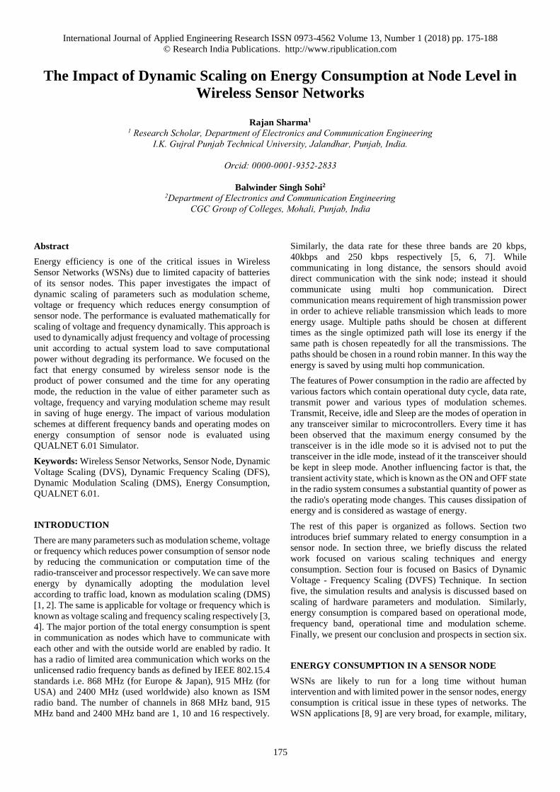
Table 6: Total charge consumed by battery (in mAhr) for various modulation schemes at different

frequencies related to Node: 9 (FFD)

Modulation Scheme Frequency Band

(In MHz)

Frequency

(In MHz)

Node ID : 9 (FFD)

Total Charge Consumed by

Battery (in mAhr)

O- QPSK 2400 - 2483.5 2400 0.35

O- QPSK 868 - 868.6 868 0.38

O- QPSK 902 - 928 915 0.35

BPSK 868 - 868.6 868 0.62

BPSK 902 - 928 915 0.52

ASK 868 - 868.6 868 0.32

ASK 902 - 928 915 0.34

Figure 10: Comparison of total charge consumed by battery (in mAhr) for various modulation schemes at different frequencies

related to node: 9 (FFD)

The Table 6 and Fig. 10 draws a comparative analysis of total

charge consumed by battery (in mAhr) for the same network

using various modulation schemes at different frequency band

related to specific node: 9 which works as Full Functional

Device (FFD). The above figure represents that the battery

charge consumption is maximum for BPSK modulation

scheme at 868 MHz and battery charge consumption is

minimum for ASK modulation scheme at 868 MHz frequency

band. The charge consumption by ASK and O-QPSK

modulation scheme is approximately same as it ranges from

0.32 to 0.38 irrespective of frequency band. The merit of using

O-QPSK modulation at 2400 MHz frequency band is high data

rate i.e. 250 kbps as compared to ASK modulation scheme at

868 MHz. The graph clearly shows that the charge

consumption in case of BPSK modulation is approximately 1.5

to 2 times higher as compared to ASK and O-QPSK which is

not recommended as energy is most precious in sensor

networks.

C. Effect of Operational Frequency Band and Modulation

Scheme on Operational Mode Time in Sensor Node

The tabular results that compares percentage of operational

time for various modulation schemes at different frequency

bands for nodes operating in transmit, receive, idle and sleep

mode are represented in the Table 7.

0.350.38

0.35

0.62

0.52

0.32 0.34

0

0.1

0.2

0.3

0.4

0.5

0.6

0.7

2400MHz

868MHz

915MHz

868MHz

915MHz

868MHz

915MHz

O- QPSK O- QPSK O- QPSK BPSK BPSK ASK ASK

Tota

l Ch

arge

Co

nsu

me

d b

y B

atte

ry (

in m

Ah

r)

Modulation Scheme and Frequency

Battery Consumption of Node: 9 (FFD)



183

Table 7: Comparison of time (in Percentage) for different modes of operation (node wise) with various modulation schemes and

frequency bands.

Modulation

Scheme

Mode Frequency

(In MHz)

Operating Time (in %) Node wise

1 (RFD) 2 (RFD) 3(RFD) 4(RFD) 5(RFD) 6(RFD) 7(RFD) 8(RFD) 9(FFD)

O- QPSK Transmit 2400 0.152693 0.149429 0.160885 0.155947 0.159531 0.156704 0.146848 0.147285 2.32992

Receive 2.18206 2.21218 2.23373 2.20415 2.34338 2.20865 2.21742 2.16893 0.877889

Idle 1.01162 1.24866 1.36234 1.18749 39.1659 1.11737 1.33876 1.29441 96.7922

Sleep

Mode

96.6536 96.3897 96.243 96.4524 58.3311 96.5173 96.297 96.3894 -

O- QPSK Transmit 868 0.387467 0.390533 0.41712 0.432907 0.46032 0.42648 0.44392 0.41392 2.88104

Receive 2.76984 2.49688 2.56496 2.80669 2.90589 2.55243 2.84579 2.52733 2.62614

Idle 38.441 3.17514 3.72685 37.357 39.2782 2.67351 42.8278 3.65485 94.4928

Sleep

Mode

58.4017 93.9374 93.2911 59.4034 57.3556 94.3476 53.8825 93.4039 -

O- QPSK Transmit 915 0.157237 0.151392 0.160885 0.159936 0.160235 0.158261 0.143456 0.144043 2.32866

Receive 2.2089 2.19499 2.24872 2.20053 2.34986 2.25033 2.19306 2.14761 0.886019

Idle 1.16849 1.44245 1.39154 1.23482 39.3922 1.25044 1.2476 1.18971 96.7853

Sleep

Mode

96.4654 96.2112 96.1988 96.4047 58.0977 96.341 96.4159 96.5186 -

BPSK Transmit 868 1.76507 1.5382 2.03827 1.14973 1.92873 1.6298 1.5126 1.7964 12.2841

Receive 9.36433 9.27873 9.63087 8.81533 11.3383 9.66547 10.0592 10.9587 11.1355

Idle 4.12284 4.20249 4.33533 3.59551 33.5445 3.58579 5.50714 32.065 76.5803

Sleep

Mode

84.7478 84.9806 83.9955 86.4394 53.1885 85.1189 82.9211 55.1799 -

BPSK Transmit 915 1.1447 1.08427 1.0816 0.991567 1.13903 0.983767 1.1155 0.966533 10.1119

Receive 9.67103 9.13434 9.11063 8.83637 9.11857 8.9014 8.95473 8.76573 5.67234

Idle 32.4637 3.22355 2.82249 2.90635 3.16359 2.87036 2.36914 2.13119 84.2158

Sleep

Mode

56.7206 86.5578 86.9853 87.2657 86.5788 87.2445 87.5606 88.1365 -

ASK Transmit 868 0.158565 0.139179 0.13696 0.165413 0.189029 0.17864 0.135845 0.119513 0.706251

Receive 0.631105 0.516582 0.533224 0.609894 0.664503 0.596374 0.56742 0.529317 0.991304

Idle 41.7252 2.17733 2.14039 42.435 40.6044 42.5773 34.3824 3.84115 98.3024

Sleep

Mode

57.4851 97.1669 97.1894 56.7897 58.5421 56.6476 64.9144 95.51 -

ASK Transmit 915 0.147877 0.143147 0.141456 0.158251 0.156123 0.153515 0.142155 0.157765 1.86073

Receive 1.935 1.75498 1.73812 1.78387 1.91984 1.78577 1.73644 1.85309 0.876158

Idle 41.5682 1.12581 1.39186 1.10018 40.1195 0.98585 1.10626 44.9305 97.2631

Sleep

Mode

56.3489 96.9761 96.7286 96.9577 57.8045 97.0749 97.0151 53.0587 -



184

Figure 11: Comparison of transmit time (in %) node wise for

different modulation schemes at 868 MHz

The graph in Fig. 11 represents the comparison of transmit time

(in %) node wise for different modulation schemes at 868 MHz

The red line clearly shows that the transmitting time is higher

using BPSK modulation scheme, blue line represents that

transmitting time is less using O-QPSK compared to BPSK.

Similarly, grey line represents that transmitting time is least

using ASK as compared to other modulation schemes such as

BPSK and O-QPSK. It also shows that the time duration for

transmission is approximately same using O-QPSK or ASK

modulation scheme in the case of RFD nodes except FFD node.

Figure 12: Comparison of receiving time (in %) node wise

for different modulation schemes at 868 MHz

The graph in Fig.12 shows the comparison of receiving time

(in %) node wise for different modulation schemes at 868 MHz

The red line clearly shows that the time for receiving is highest


receiving time is less using O-QPSK compared to BPSK.

Similarly, grey line represents that receiving time is least using

ASK as compared to BPSK and O-QPSK.

0

2

4

6

8

10

12

14

Percen

tag

e o

f ti

me

Modulation scheme & Node ID

Comparison of time duration in Transmit Mode at 868

MHz

O- QPSK Transmit mode 868 MHz

BPSK Transmit mode 868 MHz

ASK Transmit mode 868 MHz

0

2

4

6

8

10

12

Percen

tag

e o

f T

ime

Modulation Scheme & Node ID

Comparison of time duration in Receive Mode at 868

MHz

O- QPSK Receive mode 868 MHz

BPSK Receive mode 868 MHz

ASK Receive mode 868 MHz



185

Figure 13: Comparison of idle time (in %) node wise for


The Fig. 13 represents the comparison of idle time (in %) node

wise for different modulation schemes at 868 MHz. The graphs

clearly demonstrate that the idle time is on higher side in

majority of the nodes using ASK modulation scheme as

indicated by grey line. Similarly, red line represents that idle

time is least using BPSK as compared to ASK and O- QPSK.

Figure 14: Comparison of sleep time (in %) node wise for


The Fig. 14 represents the comparison of sleep time (in %) node


clearly demonstrate that the sleep time is on higher side as 5

RFD’s nodes are in the range of (93-94) % using O-QPSK

modulation scheme as indicated by blue line. The sleep time is

in the range of (83- 86) % in 6 RFD nodes using BPSK

modulation scheme. Similarly, red line represents that sleep

time in least number of nodes as only 3 nodes have high sleep

time i.e. in the range of (95- 97) % using ASK as compared to

other modulation schemes i.e. BPSK and O- QPSK. It has

been observed that sleep time for FFD node is negligible in star

topology for all the above mentioned modulation schemes.

Figure 15: Comparison of transmit time (in %) node wise for


The graph in Fig. 15 represents the comparison of transmit time

(in %) node wise for different modulation schemes at 915MHz.

The grey line clearly shows that the transmission time is on

higher side using ASK modulation scheme, red line represents

that transmission time is less using BPSK compared to ASK.

Similarly, blue line represents that transmission time is least

using O-QPSK as compared to ASK and BPSK. It also shows

that the time duration for transmitting is approximately close to

each other using all the above mentioned modulation scheme

in the case of RFD nodes except FFD node.

0

20

40

60

80

100

120

Percen

tag

e o

f T

ime


Comparison of time duration in Idle Mode at 868

MHz

O- QPSK Idle mode 868 MHz

BPSK Idle mode 868 MHz

ASK Idle mode 868 MHz

0

20

40

60

80

100

120

Percen

tag

e o

f T

ime


Comparison of time duration in Sleep Mode at 868 MHz

O- QPSK Sleep Mode 868 MHz

BPSK Sleep Mode 868 MHz

ASK Sleep Mode 868 MHz

0

1

2

3

4

5

6

7

Percen

tag

e o

f T

ime


Comparison of time duration in Transmit Mode at 915

MHz

ASK Transmit mode 915 MHz

BPSK Transmit mode 915 MHz




186

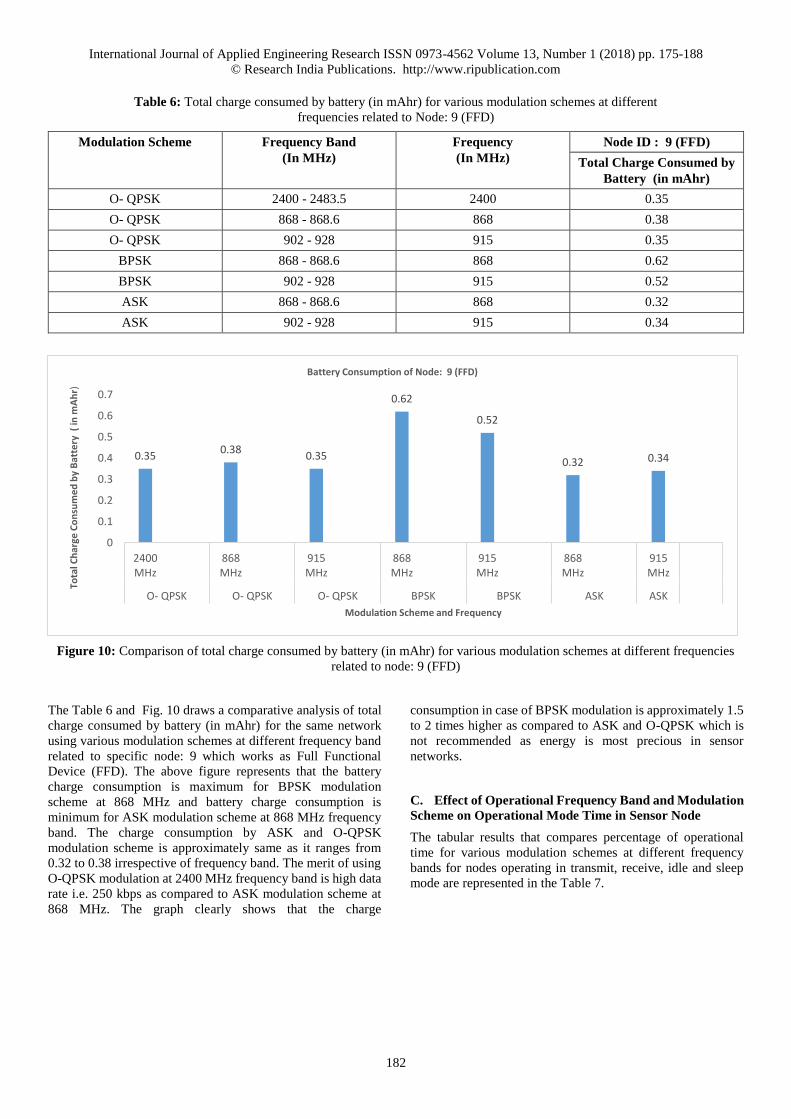
Figure 16: Comparison of receiving time (in %) node wise

for different modulation schemes at 915 MHz

The graph in Fig. 16 shows the comparison of receiving time

(in %) node wise for different modulation schemes at 915 MHz.

The red line clearly shows that the time for receiving is highest


receiving time is less using O-QPSK compared to BPSK.

Similarly, grey line represents that receiving time is least using

ASK as compared to others i.e. BPSK and O-QPSK. It is

observed that the time duration for receiving using ASK and

O-QPSK modulation scheme is approximately close to each

other in the case of RFD nodes and FFD node.

Figure 17: Comparison of idle time (in %) node wise for


The Fig. 17 represents the Comparison of idle time (in %) node


clearly demonstrate that the idle time is on higher side in

majority of the nodes using ASK modulation scheme as

indicated by grey line. Similarly, red line represents that idle

time is least in majority of nodes using BPSK as compared to

ASK and O- QPSK.

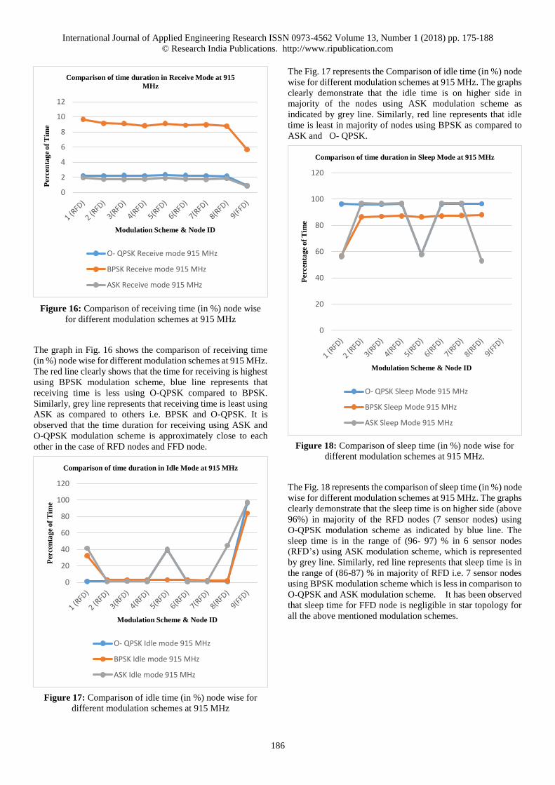
Figure 18: Comparison of sleep time (in %) node wise for

different modulation schemes at 915 MHz.

The Fig. 18 represents the comparison of sleep time (in %) node


clearly demonstrate that the sleep time is on higher side (above

96%) in majority of the RFD nodes (7 sensor nodes) using

O-QPSK modulation scheme as indicated by blue line. The

sleep time is in the range of (96- 97) % in 6 sensor nodes

(RFD’s) using ASK modulation scheme, which is represented

by grey line. Similarly, red line represents that sleep time is in

the range of (86-87) % in majority of RFD i.e. 7 sensor nodes

using BPSK modulation scheme which is less in comparison to

O-QPSK and ASK modulation scheme. It has been observed

that sleep time for FFD node is negligible in star topology for

all the above mentioned modulation schemes.

0

2

4

6

8

10

12

Percen

tag

e o

f T

ime


Comparison of time duration in Receive Mode at 915

MHz


BPSK Receive mode 915 MHz

ASK Receive mode 915 MHz

0

20

40

60

80

100

120

Percen

tag

e o

f T

ime


Comparison of time duration in Idle Mode at 915 MHz


BPSK Idle mode 915 MHz

ASK Idle mode 915 MHz

0

20

40

60

80

100

120

Percen

tag

e o

f T

ime


Comparison of time duration in Sleep Mode at 915 MHz


BPSK Sleep Mode 915 MHz

ASK Sleep Mode 915 MHz



187

Figure 19: Comparison of time (in %) for O-QPSK in

transmit, receive, idle and sleep mode at 2400 MHz

The Fig. 19 draws a comparative analysis of operational time

for various operating modes such as transmit, receive, idle and

sleep mode using O- QPSK modulation schemes at 2400 MHz

frequency band related to all RFD nodes (Node no. 1 to 8) and

specific node: 9 which works as Full Functional Device (FFD).

The above figure represents that operating time is on

comparatively higher side i.e. 96% in sleep mode for majority

of RFD’s except node no.5 which is 58% and FFD which is

zero. The energy consumption in receive mode is approximately

2% for all RFD’s except FFD. The energy consumption is

around 1% in all RFD’s except node no 5 which is 39% and for

FFD which is 96.79% in the idle mode. It is observed that

transmit time is on very lower side in comparison to sleep

mode, receive mode and idle mode.

CONCLUSION

We simulate the proposed work with 8 RFD’s and 1 FFD to

investigate the impact of various scaling techniques such as

voltage, frequency and modulation on the energy consumption

of sensor node. It is observed that for specific node i.e. node no.

9 which is Full Functional Device (FFD), the maximum battery

consumption is occurred using BPSK modulation scheme at

868 MHz and comparatively less by using BPSK modulation

scheme at 915MHz. The battery consumption using O-QPSK

modulation scheme is less as compared to BPSK modulation

scheme. In the specific case of O-QPSK, the battery

consumption is on higher side at 868 MHz compared to 915

MHz and 2400 MHz, but the energy consumption using O-

QPSK modulation is almost same for 915 MHz and 2400 MHz.

The battery consumption is least using ASK modulation

scheme as compared to other modulation scheme such as BPSK

and O-QPSK. In the specific case of using ASK, battery

consumption at 915 MHz is slightly higher compared to 868

MHz. It has been concluded that BPSK modulation is not

recommended as it decreases the battery life span of sensor

node which further reduces the lifetime of Wireless sensor

network. If we compare ASK and O-QPSK, the battery

consumption is least for ASK at 868 MHz which is

approximately same as for O-QPSK at 2400 MHz. The

advantage of using O-QPSK at 2400 MHz is higher data rate

(250 Kbps) as compared to ASK at 868 MHz whose data rate

is 20 Kbps at the cost of almost same battery consumption. The

scaling is the trade-off decision between energy efficiency node

performance according to user priority and requirement. This

work strongly recommends the necessity of using combined

DVFS – DMS approach which can significantly increase the

life span of sensor node battery. The proposed investigation

opens a lot of research gates for the future researchers to

optimize the battery consumption and to prolong sensor node

lifetime.

ABBREVIATIONS

WSNs Wireless Sensor Networks

DVS Dynamic voltage Scaling

DFS Dynamic Frequency Scaling

DVFS Dynamic Voltage and Frequency Scaling

DMS Dynamic Modulation Scaling

DPM Dynamic Power Management

USA United States of America

ISM Industrial, Scientific and Medical

CMOS Complementary Metal Oxide Semiconductor

AODV Ad hoc On-Demand Distance Vector

FFD Full Functional Device

RFD Reduced Functional Device

CBR Constant Bit Rate

ASK Amplitude-Shift Keying

BPSK Binary Phase Shift Keying

O- QPSK Offset Quadrature Phase Shift Keying

REFERENCES

[1] C. Schurgers, V. Raghunathan, and M. B. Srivastava,

"Power management for energy-aware communication

systems," ACM Transactions on Embedded Computing

Systems, vol. 2, no. 3, pp. 431-447, 2003.

[2] V. Raghunathan, C. Schurgers, S. Park, and M. B.

Srivastava, "Energyaware wireless microsensor

networks," Signal Processing Magazine, IEEE, vol. 19,

no. 2, pp. 40-50, 2002.

[3] Y. Seo, J. Kim, and E. Seo, “Effective analysis of DVFS

and DPM in mobile devices,” Journal of Computer Science and Technology, Vol. 27, No. 4, July 2012, pp.

781-790.

0

20

40

60

80

100

120

Percen

tag

e o

f T

ime

Communication mode & Node ID

Comparison of time duration in O-QPSK Transmit

Mode, Receive Mode,Idle Mode, Sleep Mode at 2400

MHz







188

[4] J. Shuja, S. A. Madani, K. Bilal, K. Hayat, S. U. Khan,

and S. Sarwar, “Energy-efficient data centers,”

Computing, Vol. 94, No. 12, 2012, pp. 973-994.

[5] QualNet 6.1Sensor Networks Model

Library,September2012, pp.14,Scalable Network

Technologies, Inc., http://www.scalable-networks.com

[6] Liu Yanfei, Wang Cheng, Qiao Xiaojun, Zhang Yunhe,

Yu chengbo,Liu Yanfei, “An Improved Design of

ZigBee Wireless Sensor Network”, IEEE 2009.

[7] Chia-Ping Huang, “Zigbee Wireless Network

Application Research Case Study Within Taiwan

University Campus”, Proceedings of the Eighth

International Conference on Machine Learning and

Cybernetics, Baoding, 12-15 July 2009.

[8] Y. Zatout, R. Kacimi, J-F. Llibre and E. Campo:

Mobility-aware Protocol for Wireless Sensor Networks

in Health-care Monitoring: Fifth IEEE: International

Workshop on Personalized Networks, USA (2011).

[9] S. Zhao and D. Raychaudhuri: Multi-tier Ad hoc Mesh

Networks with Radio Forwarding Nodes: IEEE Global

Telecommunications Conference, IEEE GLOBECOM

2007, Washington, USA (2007).

[10] M. Bandari, R. Simon and H. Aydin, "Energy

management of embedded wireless systems through

voltage and modulation scaling under probabilistic

workloads," 2014 International Green Computing Conference (IGCC), DALLAS, TX, USA, 2014, pp. 1-

10. doi:10.1109/IGCC.2014.7039168

[11] Usman, Saeeda & U. Khan, Samee & Khan, Sikandar.

(2013). A comparative study of voltage/frequency

scaling in NoC. IEEE International Conference on

Electro Information Technology. 1-5.

10.1109/EIT.2013.6632716.

[12] U. Kulau, F. Busching and L. Wolf, "A Node's Life:

Increasing WSN Lifetime by Dynamic Voltage

Scaling," 2013 IEEE 9th International Conference on Distributed Computing in Sensor Systems (DCoSS 2013) (DCOSS), Cambridge, MA, 2013, pp. 241-248.

doi:10.1109/DCOSS.2013.39

[13] Bahareh Gholamzadeh, and Hooman Nabovati,

“Concepts for Designing Low Power Wireless Sensor

Network World Academy of Science, Engineering and

Technology,” International Journal of Electronics and

Communication Engineering, Vol: 2, No: 9, 2008.

[14] R. Sharma, B.S Sohi, N. Mittal, “Hierarchical Energy

Efficient MAC protocol for Wireless Sensor Networks”.

International Journal of Applied Engineering Research,

Volume 12, Number 24, 2017, pp. 14727-14738.

[15] R. Sharma, B.S Sohi, Amar Singh and Shakti Kumar,

“ANN Based Framework for Energy Efficient Routing

In Multi-Hop WSNs”. International Journal of

Advanced Research in Computer Science, Vol. 8, No.5,

2017.

[16] R. Sharma, B.S Sohi, “A Comparative Study on MAC

Protocols for Wireless Sensor Networks on Energy

Reduction”. International Journal of Computer Science

and Information Security, 15(11), 2017, pp 35–40.

[17] H. Aydin, R. Melhem, D. Mosse, and P. Mejia-Alvarez,

"Power-aware scheduling for periodic real-time tasks,"

IEEE Trans. on Computers, vol. 53, no. 5, pp. 584-600,

2004.

[18] S. Reda, R. Cochran, and A. K. Coskun, “Adaptive

power capping for servers with multi-threaded

workloads,” International Symposium on

Microarchitecture (MICRO ‘12), Vol. 32, No. 5, Aug.

2012, pp. 64-75.

[19] C. O. Diaz, M. Guzek, J. E. Pecero, P. Bouvry, and S. U.

Khan, “Scalable and energy-efficient scheduling

techniques for large-scale systems,” International Conference on Computer and Information Technology (CIT ‘11), Sept. 2011, pp. 641-647.

[20] S. U. Khan and I. Ahmad, “A cooperative game

theoretical technique for joint optimization of energy

consumption and response time in computational grids,”

IEEE Transactions on Parallel and Distributed Systems,

Vol. 20, No. 3, Mar. 2009, pp. 346-360.

[21] S. U. Khan and N. Min-Allah, “A goal programming

based energy efficient resource allocation in data

centers,” Journal of Supercomputing, Vol. 61, No. 3,

Sept. 2012, pp. 502-519.

[22] P. Lindberg, J. Leingang, D. Lysaker, K. Bilal, S. U.

Khan, P. Bouvry, N. Ghani, N. Min-Allah, and J. Li,

“Comparison and analysis of greedy energy-efficient

scheduling algorithms for computational grids,” in

Energy Aware Distributed Computing Systems, A. Y.

Zomaya and Y.-C. Lee, Eds., John Wiley & Sons,

Hoboken, NJ, USA, 2012, ISBN 978-0-470-90875-4,

Chapter 7.

[23] W. Dargie, "Dynamic power management in wireless

sensor networks: State-of-the-art," Sensors Journal,

IEEE, vol. 12, no. 5, pp. 1518-1528, may 2012.

[24] G. L. Valentini, W. Lassonde, S. U. Khan, N. Min-

Allah, S. A. Madani, J. Li, L. Zhang, L. Wang, N. Ghani,

J. Kolodziej, H. Li, A. Y. Zomaya, C.-Z. Xu, P. Balaji,

A. Vishnu, F. Pinel, J. E. Pecero, D. Kliazovich, and P.

Bouvry, “An overview of energy efficiency techniques

in cluster computing systems,” Cluster Computing, Vol.

16, No. 1, Mar. 2013, pp. 3-15.

[25] S. Zeadally, S. U. Khan, and N. Chilamkurti, “Energy

efficient networking: past, present, and future,” Journal of Supercomputing, Vol. 62, No. 3, Dec. 2012, pp.

1093-1118.

[26] X. Jin and S. Goto, “Hilbert transform-based workload

prediction and dynamic frequency scaling for power

efficient video encoding,” IEEE Transactions on Computer-Aided Design of Integrated Circuits and Systems, Vol. 31, No.5, May 2012, pp. 649-661.

[27] U. Tietze and C. Schenk, Electronic Circuits: Handbook

for Design and Application. Secaucus, NJ, USA:

Springer-Verlag New York, Inc., 2007.

http://www.scalable-networks.com/

The Impact of Dynamic Scaling on Energy Consumption at … · · 2018-01-23Voltage Scaling (DVS),...

Documents

Transcript of The Impact of Dynamic Scaling on Energy Consumption at … · · 2018-01-23Voltage Scaling (DVS),...