The Impact of Credit Risk and Implied Volatility on Stock ...
60
The Impact of Credit Risk and Implied Volatility on Stock Returns Florian Steiger 1 Working Paper, May 2010 JEL Classification: G10, G12, G17 Abstract: This paper examines the possibility of using derivative-implied risk premia to explain stock returns. The rapid development of derivative markets has led to the possibility of trading various kinds of risks, such as credit and interest rate risk, separately from each other. This paper uses credit default swaps and equity options to determine risk premia which are then used to form portfolios that are regressed against the returns of stock portfolios. It turns out that both, credit risk and implied volatility, have high explanatory power in regard to stock returns. Especially the returns of distressed stocks are highly dependent on credit risk fluctuations. This finding leads to practical implications, such as cross-hedging opportunities between equity and credit instruments and potentially allows forecasting stock returns based on movements in the credit market. ____________ 1 Author: Florian Steiger, e-mail: [email protected]
Transcript of The Impact of Credit Risk and Implied Volatility on Stock ...
The Impact of Credit Risk and Implied Volatility
on Stock Returns
Florian Steiger1
Working Paper, May 2010
JEL Classification: G10, G12, G17
Abstract:
This paper examines the possibility of using derivative-implied risk premia to
explain stock returns. The rapid development of derivative markets has led to
the possibility of trading various kinds of risks, such as credit and interest rate
risk, separately from each other. This paper uses credit default swaps and
equity options to determine risk premia which are then used to form portfolios
that are regressed against the returns of stock portfolios. It turns out that both,
credit risk and implied volatility, have high explanatory power in regard to
stock returns. Especially the returns of distressed stocks are highly dependent
on credit risk fluctuations. This finding leads to practical implications, such as
cross-hedging opportunities between equity and credit instruments and
potentially allows forecasting stock returns based on movements in the credit
market.
____________ 1 Author: Florian Steiger, e-mail: [email protected]

Contents
Table of Figures .............................................................................................................................. I
1 Introduction ................................................................................................................................ 1
1.1 Problem Definition and Objective ....................................................................................... 1
1.2 Course of the Investigation .................................................................................................. 1
2 Asset Pricing Models and Derivative Markets ........................................................................... 2
2.1 The CAPM........................................................................................................................... 2
2.2 Multifactor Models .............................................................................................................. 6
2.3 The Advantages of Derivative Markets for Asset Pricing Models .................................... 10
3 Implied Volatility and CDS Spreads as Risk Factors ............................................................... 14
3.1 Implied Volatility .............................................................................................................. 14
3.1.1 The Black-Scholes Formula ....................................................................................... 14
3.1.2 Determining the Implied Volatility ............................................................................ 15
3.1.3 Implied Volatility and Stock Returns ......................................................................... 16
3.2 The CDS Spread and Stock Returns .................................................................................. 17
4 Impact of Credit Risk and Implied Volatility on Stock Returns .............................................. 18
4.1 Credit Risk and Implied Volatility as Risk Factors ........................................................... 18
4.2 Analytic Methodology ....................................................................................................... 18
4.2.1 Stock Universe ............................................................................................................ 18
4.2.2 Econometric Methodology ......................................................................................... 19
4.3 Determination of Risk Premia ........................................................................................... 20
4.3.1 The Risk Premium for CDS Spreads .......................................................................... 20
4.3.2 The Risk Premium for Implied Volatility ................................................................... 21
4.4 Regression Analysis .......................................................................................................... 25
4.4.1 CDS Premium ............................................................................................................. 25
4.4.2 Volatility Premium ..................................................................................................... 29
4.4.3 CDS-, Volatility-, and Market Premium..................................................................... 33
5 Summary................................................................................................................................... 37
5.1 Discussion of Results ........................................................................................................ 37
5.2 Ideas for Further Research ................................................................................................. 41
5.3 Conclusion ......................................................................................................................... 41
Bibliography ................................................................................................................................ 43
Appendix ..................................................................................................................................... 47

The Impact of Credit Risk and Implied Volatility on Stock Returns I
Table of Figures
Picture 1: CAPM - Efficient frontier ............................................................................................. 4
Picture 2: CAPM - The SML ........................................................................................................ 5
Picture 3: Negative Swap Basis Trade ........................................................................................ 13
Picture 4: VMC Daily Returns .................................................................................................... 24
Picture 5: RMU Factor Loadings of Decile Regression .............................................................. 27
Picture 6: VMC Factor Loadings of Decile Regression .............................................................. 32
Picture 7: RMU and VMC Factor Loadings of Decile Regression ............................................. 36
Table 1: Daily Summary Statistics for RMU and RM ................................................................ 20
Table 2: Annual Summary Statistics for RMU and RM ............................................................. 21
Table 3: Daily Summary Statistics for VMC .............................................................................. 22
Table 4: Annual Summary Statistics for VMC ........................................................................... 22
Table 5: VMC Time-Series Split ................................................................................................ 23
Table 6: MB Quintiles regressed against RMU .......................................................................... 25
Table 7: MB Quintiles regressed against RMU and RM ............................................................ 26
Table 8: MB Quintiles regressed against VMC .......................................................................... 30
Table 9: VMC Summary Statistics ............................................................................................. 30
Table 10: MB Quintiles regressed against VMC and RM .......................................................... 31
Table 11: MB Quintiles regressed against RMU, VMC, and RM .............................................. 33
Table 12: MB Quintiles regressed against HML, SMB, and RM ............................................... 35
Table 13: Risk Factors (Chen, Roll, & Ross, 1986).................................................................... 47
Table 14: CAPM Regression (Fama & French, 1993, p. 20) ...................................................... 48
Table 15: Fama-French - RMRF, SMB, HML (Fama & French, 1993, pp. 23-24) ................... 49
Table 16: Fama-French - TERM, DEF (Fama & French, 1993, p. 17) ...................................... 50
Table 17: Fama-French - RMRF, SML, HML, TERM, DEF (Fama & French, 1993, pp. 28-29)
.................................................................................................................................................... 51
Table 18: Carhart - Summary Statistics (Carhart, 1997, p. 77) ................................................... 52
Table 19: Carhart - Factor Loadings (Carhart, 1997, p. 64) ....................................................... 53
Table 20: Stock Universe ............................................................................................................ 54
Table 21: MB deciles against RMU and RM .............................................................................. 55
Table 22: MB deciles against VMC and RM .............................................................................. 55
Table 23: MB deciles against RMU, VMC, and RM .................................................................. 56
Table 24: MB deciles against RMU, VMC, SMB, HML, and RM ............................................ 57
Table 25: Dickey-Fuller Test on RMU and HML ...................................................................... 57

The Impact of Credit Risk and Implied Volatility on Stock Returns 1
1 Introduction
1.1 Problem Definition and Objective
This paper tries to examine the possibility of using derivative-implied risk premia to
explain stock returns. The intuition behind this approach is that the rapid development
of derivative markets within the last ten years has led to the possibility of trading
various kinds of risks, such as credit and interest rate risk, separately from each other.
Also the abundance of evidence that derivative markets react faster to news than cash
markets is advantageous to building an asset pricing model based on financial
derivatives instead of cash market products.
This approach is different to that of most classic asset pricing models such as the CAPM
and multifactor models like the Fama-French or Carhart models. These models use cash
market instruments to calculate risk premia, which are then used in a multivariate
regression to determine an asset’s sensitivity, or factor loadings, to these risk premia.
However, parts of the methodology of the classical Fama-French three factor model are
still used in the empirical part of this paper. The main difference in this paper is that the
determining factors are based on financial derivatives instead of cash market
instruments. To be specific, this paper uses the implied volatility based on equity
options and the credit risk based on credit default swap spreads as determining risk
factors in the pricing model. Ultimately, it is the objective of this paper to test if these
derivative-implied risk factors and their corresponding risk premia are sufficient to
explain stock returns. Hence, the statistical significance and the measures for the overall
explanatory power, specifically the R², of this analysis will in the end be the indications
to determine if an approach that uses derivative-implied data is successful to adequately
explain stock returns.
1.2 Course of the Investigation
In the beginning, this paper reviews the classic asset pricing theories starting with the
capital asset pricing model followed by multifactor models. Specific emphasize is being
placed on the Fama-French and the Carhart models, since they use approaches in
determining the risk premia and factor loadings that are similar to those used in this
paper. Afterwards, the theoretic advantages of using derivative markets instead of cash
markets for multivariate asset pricing models are discussed.

The Impact of Credit Risk and Implied Volatility on Stock Returns 2
In the next section, implied volatility and credit risk are introduced as risk factors.
Especially the determination of the implied volatility based on the Black-Scholes option
pricing formula is discussed together with its underlying assumptions and constraints.
Afterwards, the literature findings about possible relationships between implied
volatility, credit default swap spreads, and stock returns is reviewed.
In the following empirical section, the exact model specifications and econometric
approaches of this paper are introduced together with the selection criteria for the
relevant stocks and derivatives which are included in this study. Afterwards the
formation of the stock portfolios, against which the risk factors are later regressed, is
described. Then, in the main part of this paper, the risk premia for implied volatility and
the credit risk are determined. Following that, the factor loadings of the analyzed
portfolios on these risk premia as well as their statistical properties are derived through
a multivariate regression analysis.
The results of this regression analysis are discussed in the next section. Specific
emphasize is put on the factor loadings, their statistical significance, and the overall
explanatory power of this analysis. Afterwards, a short summary of the findings
concludes this paper together with some ideas for further research.
2 Asset Pricing Models and Derivative Markets
2.1 The CAPM
One of the most well known and widely used models to analyze stock returns is the
capital asset pricing model (CAPM) that was independently developed by William
Sharpe (1964) and John Lintner (1965). The CAPM is based on the portfolio
optimization theory by Henry Markowitz (1952), who describes portfolio selection as a
question of achieving high returns while minimizing overall portfolio risk or variance.
He argues that rational investors will always try to maximize their return whilst
minimizing their portfolio variance. The Sharpe-Ratio, which is one of the most often
used ratios in modern finance, is exactly the mathematical statement of this relationship
as it is the ratio of excess return of a portfolio to its risk, as described by its standard
deviation (Sharpe, 1966):
𝑆𝑎𝑟𝑝𝑒 − 𝑅𝑎𝑡𝑖𝑜 = 𝑅𝑖 − 𝑅𝑓
𝜎𝑖

The Impact of Credit Risk and Implied Volatility on Stock Returns 3
The progress of modern portfolio theory has led to the development of more
sophisticated models to describe this classic risk-return relationship. The Sortino ratio
for example uses one sided moments to include only the downside volatility in the
denominator. Instead of calculating the excess return against the risk-free rate, the
Sortino ratio uses an arbitrary threshold in the numerator (Sortino & Van der Meer,
1991). This threshold could be the minimum return guaranteed to outside investors or
the maximum loss a portfolio could absorb before margin calls lead to its liquidation.
𝑆𝑜𝑟𝑡𝑖𝑛𝑜 − 𝑅𝑎𝑡𝑖𝑜 = 𝑅𝑖 − 𝑇
𝜃𝑖(𝑡)
where
𝜃𝑖(𝑡) = 𝑡 − 𝑟𝑝 2𝑝𝑑𝑓(𝑟𝑝 )𝑑𝑟𝑝
𝑡
∞
0.5
Even though formulas have become more complex since the first approaches were made
by Markowitz, the idea of return maximization and risk minimization is still one of the
underlying concepts of modern finance. Hence, the CAPM, which is based on these
very fundamentals, is still of practical and theoretical use. In order to understand more
advanced asset pricing models, the CAPM is quickly introduced in this section.
The CAPM is an equilibrium based model which assumes that all investors agree on the
distribution of asset returns and that all investors hold efficient frontier portfolios. A
portfolio on the efficient frontier is the portfolio with the highest possible return for a
given standard deviation. The CAPM furthermore assumes that there is a risk-free asset
paying the interest rate 𝑅𝑓 which can also be used to borrow money at the same rate.
Asset demand and asset supply are in equilibrium in the CAPM.
These assumptions lead to several implications: The most important implication is that
the portfolio with the highest Sharpe-Ratio, also known as the tangent portfolio, is the
market portfolio.

The Impact of Credit Risk and Implied Volatility on Stock Returns 4
Picture 1: CAPM - Efficient frontier
The second implication, also known as Tobin separation theorem, is that all investors
hold the market portfolio. The only difference between investors with different utility
functions is the overall proportion of their wealth which they invest into the market
portfolio and into the risk-free asset.
The CAPM further states that the return of a risky asset only depends on this asset’s
sensitivity to market risk. This sensitivity is commonly known as a stock’s beta. This
beta can be derived as follows. In equilibrium, the marginal return-to-risk of a risky
asset (𝑅𝑅𝑅𝑖) must be identical to the return-to-risk of the tangent or market portfolio
(𝑅𝑅𝑅𝑀).
Where
𝑅𝑅𝑅𝑖 =𝑟𝑖 −𝑟𝑓
𝜎𝑖𝑀 /𝜎𝑀
𝑅𝑅𝑅𝑀 =𝑟𝑀 − 𝑟𝑓
𝜎𝑀
Setting these two equal and solving for the excess return yields:
𝑟𝑖 − 𝑟𝑓 =𝜎𝑖𝑀𝜎𝑀2
𝑟𝑀 − 𝑟𝑓

The Impact of Credit Risk and Implied Volatility on Stock Returns 5
Substituting 𝛽𝑖 = 𝜎𝑖𝑀
𝜎𝑀 2 yields:
𝑟𝑖 − 𝑟𝑓 = 𝛽𝑖 𝑟𝑀 − 𝑟𝑓
This formula states that a security’s excess return is fully dependent on its systematic
risk and that idiosyncratic risk is not being rewarded. As discussed, the beta of a
security is the sensitivity to systematic risk. Securities with higher betas have higher
expected returns and vice-versa. This relationship between betas and expected return is
known as the security market line (SML).
Picture 2: CAPM - The SML
This line states that higher returns are associated with higher market betas, hence higher
systematic or market risk. This relationship is linear in its nature and assets that are not
exposed to any systematic or market risk have an expected return that is equal to the
risk-free interest rate.
So if the CAPM holds, a security’s return would be fully determined by its beta. This
testable implication does not hold very well in practice. Black, Jensen, and Scholes
(1972) have shown that the expected return of an asset is not strictly proportional to its
𝛽 and hence, that the CAPM does not hold perfectly. The CAPM can be empirically
tested using the following equation (Black, Jensen, & Scholes, 1972, p. 4), where the
alpha is the stock’s abnormal return not explained by the CAPM equation:
𝛼 = 𝐸 𝑅𝑗 − 𝐸(𝑅𝑚 )𝛽𝑗
If the CAPM accurately described the stock’s returns, alpha in this equation should not
be statistically significant different from zero. In their study, Black, Jenson, and Scholes
show that non-zero alphas, which are statistically significant, occur frequently
throughout their sample (Black, Jensen, & Scholes, 1972, p. 16). Thus the CAPM does

The Impact of Credit Risk and Implied Volatility on Stock Returns 6
not perfectly hold in all cases and can be rejected as an all-explaining model of stock
returns. This fact is also underlined by Merton’s (1973) Intertemporal Capital Asset
Pricing Model (ICAPM), which finds that the expected excess return of a risky asset
may be different from zero even if the asset bears no systematic or market risk.
However, the ICAPM is also not able to fully explain the empirical discrepancies found
in the Black, Jenson, and Scholes study (Merton, 1973, p. 885) .
Another piece of evidence that the CAPM does not accurately describe stock returns is
the fact that it is possible to forecast stock returns based on scaled price ratios, such as
price-earnings or price-dividend ratios. According to the CAPM, only the systematic
risk of a stock determines its expected return and hence, a forecast based on other
factors should not be working. Campbell and Shiller (1988) show in their study that
stock prices can indeed be predicted over the long-term using price-to-earnings ratios
(p. 675) thus rejecting the CAPM hypothesis.
To summarize: The CAPM is a powerful tool to describe stock returns, but multiple
studies have proven that it fails to explain several anomalies which result in statistically
significant abnormal returns. In order to increase the explanatory power of asset pricing
models, more factors are needed to account for the various effects which cannot be
explained by a stock’s beta. Multifactor models have been trying to overcome this
problem with some success.
2.2 Multifactor Models
As discussed above, the CAPM as single-factor model fails to completely explain stock
returns. To overcome this problem, multifactor models have been developed that use
additional factors besides the market premium to explain stock returns. Consequently,
an asset also has more than one factor loading, depending on the specific number of
factors used.
A general theoretical framework for these multifactor approaches is the Arbitrage
Theory of Capital Asset Pricing (APT) which was proposed by Ross (1976). Ross
proposed that the expected return of a specific asset depends on a multitude of risk
factors other than the single risk factor used by the CAPM (Ross, 1976, p. 355).
𝐸𝑀 = 𝜉𝑖𝐸𝑖𝑖

The Impact of Credit Risk and Implied Volatility on Stock Returns 7
Where 𝐸𝑀 is the expected return, 𝜉𝑖 is the asset’s sensitivity to the specific risk factor,
and 𝐸𝑖 is the expected risk premium that arises from bearing that specific risk.
Chen, Roll, and Ross (1986) propose a set of macroeconomic variables that are to be
used as risk factors in such a multivariate arbitrage pricing model. Examples for such
risk factors would be the industrial production, unexpected inflation, or the term
structure of interest rates. The complete set of variables examined in the Chen, Roll, and
Ross paper can be seen in table 13 in the appendix. Due to their high explanatory
power, macroeconomic variables are also used in other studies, such as in an attempt to
describe the stochastic structure of asset prices (Cox, Ingersoll, & Ross, 1985, p. 383).
Another approach besides using macroeconomic factors to explain stock returns is the
usage of variables which can be directly derived from stock returns or fundamental data.
For example, an empirical study by Fama and French (1992) has examined the effects
of a company’s size, its book-to-market equity ratio, and its earnings-to-price ratio in
order to build a multifactor asset pricing model that uses these factors as explanatory
variables. Fama and French started with the classical CAPM equation, which is shown
below:2
𝑅𝑖 − 𝑅𝑓 = 𝛼𝑖 + 𝑏𝑖 𝑅𝑀𝑅𝐹 + 𝜀𝑖
As previously discussed, there is an abundance of evidence that the CAPM ignores
other risk factors affecting stock returns, such as the just discussed value and size
effects of companies. This results in a relatively low explanatory power of this
regression. As shown in table 14 in the appendix, the R² of this regression is relatively
low with values around 0.80. In order to account for the effects of size and value on
stock returns, Fama and French expanded the model and included two additional stock
market factors that control for size and value effects (Fama & French, 1993, pp. 24-25).
This three factor equation is shown below3:
𝑅𝑖 − 𝑅𝑓 = 𝛼𝑖 + 𝑏𝑖 𝑅𝑀𝑅𝐹 + 𝑠𝑖 𝑆𝑀𝐵 + 𝑖 𝐻𝑀𝐿 + 𝜀𝑖
The SMB and HML factors are generated by sorting the whole universe of stocks into
portfolios based on their size or market capitalization and their equity book-to-market
____________ 2 RMRF = Excess market return
3 SMB = Small minus big
HML = High minus low

The Impact of Credit Risk and Implied Volatility on Stock Returns 8
ratios. Then, the return of the least risky portfolio is subtracted from the return of the
most risky portfolio. The resulting difference in returns is the risk premium that enters
the regression equation. As shown in table 15 in the appendix, both newly added factors
have statistically significant factor loadings with most t-statistics larger than 2.0 and
also the R² of the regression increases to values mostly about 0.90.
In order to evaluate if stock returns can also be explained by bond market factors, Fama
and French use a term structure premium as well as a credit risk premium as
independent variables in a two-factor model to explain stock returns. The equation is
shown below4:
𝑅𝑖 − 𝑅𝑓 = 𝛼𝑖 + 𝑚𝑖 𝑇𝐸𝑅𝑀 + 𝑑𝑖 𝐷𝐸𝐹 + 𝜀𝑖
The term structure premium is calculated as the difference in yield between long-term
government bonds and the treasury-bill rate. The default risk premium is the difference
between CB, which is a market proxy for average corporate bond yields, and the long-
term government bond yield. Economically, this could be understood as the average
credit spread of the market portfolio of debt.
The factor loadings and the corresponding t-statistics of this regression are shown in
table 16 in the appendix. As shown in the table, the factor loadings are all non-zero and
statistically highly significant with some t-statistics beyond 9.0. However, the
explanatory power of this regression seems to be quite small with R² values below 0.20.
Nonetheless, it is still notable that bond market factors explain at least some of the
variation in stock returns. This result is also supported by the study of Chen, Roll, and
Ross who find that both, the TERM as well as the DEF5 factor have some explanatory
power (Chen, Roll, & Ross, 1986, p. 402).
Fama and French consequently introduce a five factor model that uses both, stock and
bond market factors, as variables to explain stock returns. The resulting equation is
shown below (Fama & French, 1993, p. 28):
𝑅𝑖 − 𝑅𝑓 = 𝛼𝑖 + 𝑏𝑖 𝑅𝑀𝑅𝐹 + 𝑠𝑖 𝑆𝑀𝐵 + 𝑖 𝐻𝑀𝐿 + 𝑚𝑖 𝑇𝐸𝑅𝑀 + 𝑑𝑖 𝐷𝐸𝐹 + 𝜀𝑖
____________ 4 TERM = Term structure premium
DEF = Credit risk premium 5 Chen, Roll, and Ross calculate the DEF factor as difference in yield between Baa-rated bonds
and long-term government bonds. This is slightly different to the Fama-French methodology.

The Impact of Credit Risk and Implied Volatility on Stock Returns 9
The risk premia which are used as factors in this regression are determined as
previously discussed. The results of this regression can be seen in table 17 in the
appendix. In this regression that includes stock as well as bond market factors the
statistical significance of the factor loadings on TERM and DEF largely disappears with
t-statistics mostly below 2.0. The significance of the RMRF, SMB, and HML factors
however persists in this equation with some t-statistics beyond 50. Fama and French
conclude that the statistical insignificance of TERM and DEF in this regression is due to
the fact that RMRF captures most of the effects associated in these factors (Fama &
French, 1993, p. 52). The fact that the TERM factor has a positive correlation of 0.37 to
RMRF underlines this interpretation (Fama & French, 1993, p. 14). Also the R² of this
regression increases only slightly compared to the previous three factor equation.
Another possible return explaining factor was identified by Jegadeesh and Titman
(1993) in their study about momentum effects. Jegadeesh and Titman find that
momentum portfolios, which buy stocks that gained in value during the last 12 months
and short-sell stocks that lost in value during the last 12 months, generate abnormal
returns not explained by systematic risk, size, or value factors. For example, a strategy
which select stocks based on their past 6 month returns and holds them for 6 months
realizes an average compounded excess return of 12.01% per year (Jegadeesh &
Titman, 1993, p. 89). DeBondt and Thaler (1985) attribute this effect to substantial
violations of weak market efficiency due to overreactions by investors to unexpected
and dramatic events. DeLong, Shleifer, Summers, and Waldman (1990) have expended
this view by adding that some investors knowingly try to front-run momentum effects
therefore amplifying them creating a self-fulfilling prophecy. Hence, even though there
might be no rational explanation for momentum effects, it is evident that these effects
do exist in capital markets and should therefore be included in multifactor models trying
to explain stock returns.
Carhart (1997) expands the Fama-French three factor model by adding such a factor that
accounts for momentum effects in a study on mutual fund returns. The factor, PR1YR6,
is constructed as “the equal-weight average of firms with the highest 30 percent eleven-
month returns lagged one month minus the equal-weight average of firms with the
lowest 30 percent eleven-month returns lagged one month” (Carhart, 1997, p. 61). The
____________ 6 PR1YR = Previous 1 year performance

The Impact of Credit Risk and Implied Volatility on Stock Returns 10
intuition of excluding the last month’s return in this analysis is to make sure that no
short-term reversals are included in this factor. The resulting multifactor regression
equation is shown below (Carhart, 1997, p. 61):
𝑅𝑖 = 𝛼𝑖 + 𝑏𝑖 𝑅𝑀𝑅𝐹 + 𝑠𝑖 𝑆𝑀𝐵 + 𝑖 𝐻𝑀𝐿 + 𝑝𝑖(𝑃𝑅1𝑌𝑅) + 𝜀𝑖
This model works well with statistically significant factor loadings on all risk factors
and is thus a useful extension to the traditional three factor model proposed by Fama
and French (1993). The summary statistics of this four-factor model are shown in table
18 in the appendix. The resulting factor loadings and the adjusted R² are depicted in
table 19 in the appendix. The factor loadings are statistically highly significant for most
factors in most portfolios. Also the adjusted R² values are very high with values mostly
beyond 0.90. Another interesting finding of Carhart’s study is that when regressing
mutual fund returns against this four-factor model, most funds systematically
underperform and generate negative alphas which are statistically significant with some
t-statistics beyond 3.0 (Carhart, 1997, p. 77). This result indicates that instead of hiring
a fund manager, an investor would be better off by buying mimicking portfolios that
track the four risk factors. This result becomes even more significant when accounting
for fund management costs and transaction fees.
To conclude: The above examples as well as many other studies have revealed that
multifactor models are a good method to explain stock returns and their causing factors.
Multifactor models help to resolve anomalies not explained by the CAPM and have
consistently higher R² than the classic CAPM regressions. Specific attention should
however be paid to selecting the right factors and drawing the right conclusion from a
specific factor. The danger of omitted variable bias can easily lead to statistical
significant factor loadings although the true causal effect might be different. This
danger is especially high if risk factors are highly correlated to each other.
2.3 The Advantages of Derivative Markets for Asset Pricing Models
In the last decade, derivative markets have grown significantly in size, product variety,
and liquidity. Within some market segments, the notional value of outstanding
derivatives is almost as large as or sometimes even larger than the face value of the
underlying cash securities. Especially the credit default swap market has grown
tremendously and is now one of the biggest and most liquid derivative markets. Recent
studies estimate the notional value of outstanding CDS contracts as of December 2008

The Impact of Credit Risk and Implied Volatility on Stock Returns 11
at over USD 41 trillion (European Central Bank, 2009, p. 4), other studies estimate an
even higher notional value of about USD 58 trillion (US Securities and Exchange
Commission, 2008).
This development and the growing importance of derivative markets for private as well
as for institutional investors have generated new opportunities to trade various kinds of
risks. The growing popularity of derivative markets can be attributed to an especially
useful characteristic of financial derivatives. Whereas a cash market instruments usually
bears a bundle of different risks, financial derivatives allow for the separate trading of
these various risk kinds. For example, a traditional cash market bond is usually exposed
to credit, interest rate, and currency risk. In the derivative market, all these kinds of
risks can be traded separately from each other through the use of credit default swaps,
interest rate swaps, and currency swaps or options. All of these products have the
pleasant characteristic that they are virtually uncorrelated to the other risk types. For
example, a credit default swap has almost no interest rate sensitivity. This separation of
risk is especially useful for hedging applications. An investor who wants to hedge
against rising interest rates can simply do so by entering an interest rate swap
agreement. Using traditional cash market bonds, he would have to buy a floating rate
note and finance this by issuing a fixed coupon bond. The payoff of the interest rate
swap agreement and the cash market replication strategy are identical, but the
complexity and transaction costs of the derivative transaction are much lower.
This separated trading of different risk types should also allow for interesting extensions
of the previous discussed multifactor models. Since the returns of derivatives depend on
risks which are almost uncorrelated to each other, introducing a multifactor risk model
based on derivatives could improve forecasting power and minimize omitted variable
bias. Since omitted variable bias occurs when an included factor is correlated to an
omitted factor, the use of uncorrelated factors would help to overcome this problem.
Also the traditional problem of not being able to distinguish between correlation and
causality could be reduced since derivatives, at least to a large extent, only derive their
value from only one specific kind of risk.
The faster absorption of news events in derivative markets is another advantage of using
derivative implied factors as risk proxies in asset pricing models. An example for such a
shorter reaction period is the lead-lag relationship of index futures to their respective

The Impact of Credit Risk and Implied Volatility on Stock Returns 12
indexes, where future price movements lead index movements by several minutes
(Kawaller, Koch, & Koch, 1987, p. 1309). A similar argument could be constructed for
the CDS market, which tends to react faster to news than the bond cash market (Daniels
& Jensen, 2005, p. 31). Furthermore, derivative markets sometimes do not only react
faster to certain events than cash markets, but they also price the same kind of risk
differently than cash markets.
An empirical indicator for such a divergence of risk pricing between derivative and cash
markets is the frequent possibility of negative default swap basis trades. The default
swap basis is defined as the difference between the CDS spread and the cash LIBOR
spread of a fixed income security, such as a fixed rate bond or a floating rate note
(Fabozzi, 2005, p. 1347):
𝐷𝑒𝑓𝑎𝑢𝑙𝑡 𝑆𝑤𝑎𝑝 𝐵𝑎𝑠𝑒 = 𝐶𝐷𝑆 𝑆𝑝𝑟𝑒𝑎𝑑 − 𝐶𝑎𝑠 𝐿𝐼𝐵𝑂𝑅 𝑆𝑝𝑟𝑒𝑎𝑑
According to classic economic theory, the default swap basis should be close to zero or
positive to prevent arbitrage opportunities. Bearing the credit risk in form of a long
position in a bond should yield the same return as bearing it in the form of selling a
CDS. This also implies that holding a long position in a bond and insuring this position
against default using a CDS should never yield more than the risk-free rate as return. If
the CDS spread traded below the cash LIBOR spread, buying a bond in the cash market
and insuring it against default would yield more than risk-free rate and thus result in an
arbitrage opportunity. An example for such a trade is given below.
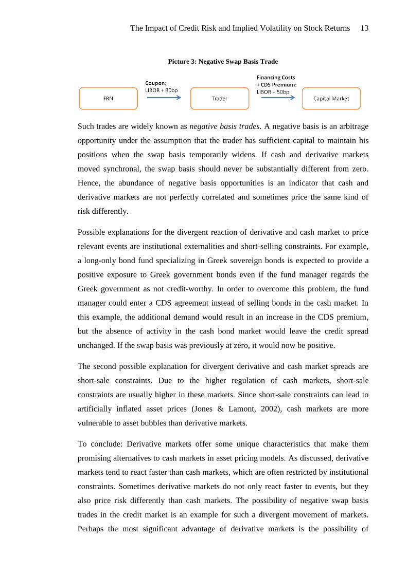
Assume a trader, who is able to refinance at LIBOR, has identified a floating rate note
(FRN) paying LIBOR + 80bp p.a. and a counterparty willing to enter a CDS agreement
with him at an annual CDS premium of 50bp. In this case, the trader could buy the bond
and reinsure it against default and thus convert his long credit exposure into a virtually
risk-free position7. Theoretically, he should earn the risk-free rate on this position, but
the negative default swap basis allows him to make 30bp profit on this zero-cost
portfolio. Clearly, this arbitrage opportunity should not exist in perfectly efficient
capital markets.
____________ 7 An additional assumption of this example is that the CDS counterparty is posting sufficient
collateral so that counterparty risk can be neglected. This trade would, however, still not be perfectly risk-
free since the trader is still exposed to the annuity risk that the bond issuer defaults before maturity.
The Impact of Credit Risk and Implied Volatility on Stock Returns 13
Picture 3: Negative Swap Basis Trade
Such trades are widely known as negative basis trades. A negative basis is an arbitrage
opportunity under the assumption that the trader has sufficient capital to maintain his
positions when the swap basis temporarily widens. If cash and derivative markets
moved synchronal, the swap basis should never be substantially different from zero.
Hence, the abundance of negative basis opportunities is an indicator that cash and
derivative markets are not perfectly correlated and sometimes price the same kind of
risk differently.
Possible explanations for the divergent reaction of derivative and cash market to price
relevant events are institutional externalities and short-selling constraints. For example,
a long-only bond fund specializing in Greek sovereign bonds is expected to provide a
positive exposure to Greek government bonds even if the fund manager regards the
Greek government as not credit-worthy. In order to overcome this problem, the fund
manager could enter a CDS agreement instead of selling bonds in the cash market. In
this example, the additional demand would result in an increase in the CDS premium,
but the absence of activity in the cash bond market would leave the credit spread
unchanged. If the swap basis was previously at zero, it would now be positive.
The second possible explanation for divergent derivative and cash market spreads are
short-sale constraints. Due to the higher regulation of cash markets, short-sale
constraints are usually higher in these markets. Since short-sale constraints can lead to
artificially inflated asset prices (Jones & Lamont, 2002), cash markets are more
vulnerable to asset bubbles than derivative markets.
To conclude: Derivative markets offer some unique characteristics that make them
promising alternatives to cash markets in asset pricing models. As discussed, derivative
markets tend to react faster than cash markets, which are often restricted by institutional
constraints. Sometimes derivative markets do not only react faster to events, but they
also price risk differently than cash markets. The possibility of negative swap basis
trades in the credit market is an example for such a divergent movement of markets.
Perhaps the most significant advantage of derivative markets is the possibility of

The Impact of Credit Risk and Implied Volatility on Stock Returns 14
separating risk into smaller tradable risk types, which have only low sensitivities to each
other. This is especially useful for multifactor models that require risk factors to be
uncorrelated to each other. However, the fact that many derivative products are only
traded in intransparent over-the-counter (OTC) markets is a disadvantage that should be
kept in mind when using derivatives in asset pricing models. Sometimes it can be very
difficult to gather the relevant information and even then it can be subject to massive
biases.
3 Implied Volatility and CDS Spreads as Risk Factors
As a consequence of the rapid development of derivative markets, derivative
instruments on almost all large-cap stocks and bonds are now available for trading. Two
of the most important derivatives, according to their liquidity and trading volume, are
equity options and credit default swaps. This paper utilizes these two products as base
products for a multifactor stock pricing model. The model uses equity options to
determine the implied volatility of a stock and the CDS spread to assess a company’s
credit riskiness or probability of default. Using these two products has some advantages:
First, equity options as well as CDS are widely available for a large range of companies
and are usually liquidly traded. The second advantage is that these products are
standardized contracts8, which eliminates the necessity of pre-processing large amounts
of data before using them in an asset pricing model.
3.1 Implied Volatility
3.1.1 The Black-Scholes Formula
A standard model to calculate the implied volatility through equity option prices is
based on the theories by Fischer Black and Myron Scholes (1973) as well as by Robert
C. Merton (1973). Consequently, this model is widely referred to as the Merton-Black-
Scholes model, for which the two then living authors Merton and Scholes received the
Nobel Prize for economics in 1997. The Black-Scholes formula determines the price of
a non-dividend paying European call option (C) based on its time to maturity (T), the
spot price of the underlying asset (𝑆0), the option’s strike price (K), the risk-free interest
rate (r), and the volatility (𝜎) of the underlying asset (Hull, 2009, p. 291):
____________ 8 Technically, only equity options traded on stock exchanges such as the Eurex or the CBOT are
standardized contracts. CDS, which are not traded on stock exchanges, are not necessarily standardized.
However, many market participants use the standardized master agreement proposed by the International
Swaps and Derivatives Organization (2010).

The Impact of Credit Risk and Implied Volatility on Stock Returns 15
𝐶 = 𝑆0𝑁 𝑑1 − 𝐾𝑒−𝑟𝑡𝑁(𝑑2)
Where
𝑁 𝑥 = Φ 𝑥 = 𝑐𝑑𝑓 𝑜𝑓 𝑎 𝑠𝑡𝑎𝑛𝑑𝑎𝑟𝑑𝑖𝑧𝑒𝑑 𝑛𝑜𝑟𝑚𝑎𝑙 𝑑𝑖𝑠𝑡𝑟𝑖𝑏𝑢𝑡𝑖𝑜𝑛
𝑑1 =ln S0 K + r +
σ2
2 𝑇
σ T
𝑑2 =ln S0 K + r −
σ2
2 𝑇
σ T= 𝑑1 − σ T
The put price can be estimated through a similar function or through the application of
the put-call parity, which states that the price of a put option can be derived from the
price of a call option with identical strike price and maturity or (Hull, 2009, p. 208):
𝑐 + 𝐾𝑒−𝑟𝑡 = 𝑝 + 𝑆0
Economically, this means that buying a stock and hedging it against losses with a put
option should have the same expected payoff as buying a call option and investing the
remaining capital in the risk-free asset.
3.1.2 Determining the Implied Volatility
All parameters of the Black-Scholes pricing formula are known in advance, except the
volatility since it is not the historical volatility which is relevant for the price
determination, but the expected future volatility. The volatility which is implied by the
option price is hence known as the implied volatility (Hull, 2009, p. 296). In order to
determine this implied volatility, traders accept the price of an option as given and then
back-solve for the implied volatility that sets equal both sides of the Black-Scholes
equation. In practice however, algebraic back-solving is not sufficient to determine the
implied volatility of more complex options, such as American options. Also the
assumptions of the Black-Scholes model, such as a constant risk-free interest rate,
constant implied volatility, or absence of dividend payments make it necessary for
traders to use more complex approaches to determine option prices or implied
volatilities, such as the implied volatility function (IVF) model developed by Derman
and Kani (1994), Dupire (1994), and Rubinstein (1994).

The Impact of Credit Risk and Implied Volatility on Stock Returns 16
For the scope of this paper however, it is sufficient to use implied volatility data that is
calculated under the simplifying assumptions of the Black-Scholes formula. For further
future studies, more complex implied volatility determination methods could
theoretically be applied in order to gain more exact and accurate results.
3.1.3 Implied Volatility and Stock Returns
In order to be a useful factor to explaining stock returns, implied volatility should have
significant effects on stock returns. Recalling the classic positive relationship between
risk and return, it seems obvious that higher expected risk would result in higher
expected returns:
𝐸 𝜎𝑡 ~𝐸(𝑟𝑡)
Yet, empirical results trying to test this relationship are somewhat inconclusive.
Cambell and Hentschel (1992) and French, Schwert, and Stambaugh (1986) find
evidence for a positive correlation between expected returns and expected risk, whereas
Glosten, Jagannathan, and Runkle (1993) find a negative relationship between these two
factors.
Due to the fact that a single asset always bears some non-systematic risk to a certain
extent, both findings do not necessarily oppose classic economic theories which state
that only systematic risk is being rewarded.
𝑉𝑎𝑟 𝑟 𝑖 = 𝛽𝑖𝑀2 𝑉𝑎𝑟 𝑟 𝑚 + 𝑉𝑎𝑟 𝜖 𝑖
Due to the fact that an expected increase in volatility cannot ad-hoc be appointed to the
systematic or the non-systematic component of total risk, no prediction based on
implied volatility about the development of future returns can be made under the
assumption that only systematic risk is being rewarded. The effect on the stock’s return
would depend on how much of the expected risk can be allocated to the systematic
component of the total risk. If one was able to forecast only the systematic portion of
the overall risk, return forecasts based on this systematic risk should theoretically be
possible. Nonetheless, since markets are not perfectly efficient, any a-priori statement
about the development of future returns would still be difficult. The regression analysis
later in this paper will hopefully generate some insights about the relationship between
implied volatility and stock returns and about the possibility of using implied volatilities
as asset pricing factor.
The Impact of Credit Risk and Implied Volatility on Stock Returns 17
3.2 The CDS Spread and Stock Returns
The second factor which is used in this paper to explain stock returns is the credit risk of
the specific company. Specifically, the CDS spread of the company over LIBOR is used
as proxy to determine the credit risk. Numerous papers have identified factors, such as
the dividend payout ratio (Lamont, 1998), which are correlated to stock returns as well
as bond yields. These findings are an implication that stock and bond returns are either
directly correlated to each other or correlated to each other through external factors. If
that was true, bond market factors could indeed be helpful in explaining stock returns.
Fama and French (Fama & French, 1989, p. 48) find that the default premium on bonds
can help to explain stock returns due to the fact that it is correlated with other relevant
factors, such as the dividend yield or the overall business cycle. It is likely that a credit
risk factor is also highly correlated to other commonly used factors to explain stock
returns. Especially the HML factor of the Fama-French model, which is a proxy for the
market valuation of a company’s equity, is a candidate for such a relationship since it
can be seen as a distressed factor (Fama & French, 1998) which should also be picked
up by higher default expectations in the bond market. Newer studies go even further in
examining the relationship between the stock and the bond market and try to explain
CDS spreads using equity options (Zhang, Zhou, & Zhu, 2009). Also the development
of joint frameworks for the valuation and estimation of stock options and CDS (Carr &
Wu, 2009) indicate a close relationship of stock and bond markets. Norden and Weber
(2009) have not only found a strong relationship between these markets, but also found
that stock returns are significantly negatively correlated with CDS and bond yield
changes (p. 554). However, it remains to be seen if those results, which origin from a
small sample and a very limited observation period, apply to more general test settings.
All these theories and studies have shown significant evidence that relationship patterns
exist between the stock and the bond market. This paper will therefore use the CDS
spread as risk factor to account for the market’s perception of the credit worthiness of
the specific company. If credit worthiness affected the stock price development, it
should be reflected in a statistically significant factor loading on the CDS factor in the
upcoming multivariate regression model.
The Impact of Credit Risk and Implied Volatility on Stock Returns 18
4 Impact of Credit Risk and Implied Volatility on Stock Returns
4.1 Credit Risk and Implied Volatility as Risk Factors
As discussed before, this paper tries to explain stock returns through factors based on
the CDS spread of a company and its equity option implied volatility. Previous theories
have already analyzed the effect of credit spreads on stock returns and found a positive
relationship between credit risk and stock returns. The following section further
advances on this topic by using credit default swap spreads as input to calculate a CDS
spread risk premium. The corresponding factor loadings are determined through a
multivariate regression analysis. If successful and in line with previous studies, the
regression model developed in this paper should also pick up a positive return premium
for stocks with higher credit risk. Special emphasis in this paper is also paid to the
distribution of the factor loadings according to a stocks market-to-book ratio, which is a
proxy for a stock’s value-effect as described by Fama and French (1993) and others. The
effect of implied volatility on stock returns has also been studied before with ambivalent
results. Some studies found positive effects of higher implied volatility on stock returns
whilst other studies have concluded that there is no measurable effect or even a negative
effect. In order to resolve this problem, this paper first determines the risk premium of
higher implied volatility and then estimates factor loadings on this factor.
4.2 Analytic Methodology
4.2.1 Stock Universe
The core universe used in this paper consists of the stocks included in the Standard &
Poor’s 100 Index, commonly referred to as the S&P 100. The intention of using this
index is that the stocks of its 100 constituent companies are very liquidly traded and that
equity as well as credit derivatives are easily available. However, credit default swap
data with sufficient quality is only available for 83 of these 100 companies; hence the
universe has to be reduced to these 83 companies. Please see table 20 in the appendix
for the complete list of stocks and the corresponding credit default swaps which were
used for this paper.
When available, standard CDS contracts with a five year maturity are used. However,
for some companies only CDS with different maturities are actively traded. In these
cases, the CDS with the closest maturity to five years are used instead. Equity options
are easily available for all companies in the S&P 100 Index. In order to gather the

The Impact of Credit Risk and Implied Volatility on Stock Returns 19
implied volatility, the implied volatility of at the money call options is used9, thereby
ignoring possible relationships between different strike prices and different implied
volatilities, known as volatility smiles. Nonetheless, for the purpose of this paper and
for the sake of simplicity, the assumption of constant implied volatilities across different
strike prices should have no significant effect on the research results10
.
The data for the implied volatilities is only available from May 15th
2008 to January 15th
2009, therefore drastically reducing the external validity of any results since only a very
small timeframe can be analyzed. The data for stock prices and CDS spreads is easily
available over a five year time horizon, which is used for any analyses that do not
include factors based on the implied volatility.
4.2.2 Econometric Methodology
The main econometrical method used in this paper is the multivariate regression
analysis. Where appropriate, the sample is broken down into quintiles or deciles to
account for possible differences in factor loadings across different portfolios. In all
regression analyses, HAC standard errors are used to control for heteroskedasticity and
autocorrelation.
The general approach of building the regression model used in this paper is to first
calculate the risk premia for stocks with higher credit default swap spreads and higher
implied volatilities. These risk premia are determined by subtracting the equal weighted
average return of stocks with the lowest CDS premia or implied volatility from those
stocks with the highest CDS and implied volatility risk premia.
𝑅𝑖𝑠𝑘 𝑃𝑟𝑒𝑚𝑖𝑢𝑚 = 𝑅𝑒𝑡𝑢𝑟𝑛𝐻𝑖𝑔−𝑟𝑖𝑠𝑘 𝑠𝑡𝑜𝑐𝑘𝑠 − 𝑅𝑒𝑡𝑢𝑟𝑛𝐿𝑜𝑤−𝑟𝑖𝑠𝑘 𝑠𝑡𝑜𝑐𝑘𝑠
The second step in building the regression model is to create quantile portfolios of
stocks against which the risk premia are regressed. Since this paper tries to examine
effects which are probably highly correlated to the market-to-book (MB) ratio of a
company’s equity, the portfolios are created with the MB ratio as sorting criteria. The
____________ 9 The implied volatility used in this paper is the implied volatility which is supplied by the
DataStream Financial Database, which uses a standard Black-Scholes model for its determination. This
method uses call options with at or near the money strike prices. 10
An effect that might be significant is the lack of transparency in the pricing of CDS contracts.
Since CDS are OTC traded products, it is possible that the quoted spreads by market makers, which are
used in this paper, do not appropriately reflect the true spreads agreed on in large OTC transactions.

The Impact of Credit Risk and Implied Volatility on Stock Returns 20
stocks with the lowest MB ratio enter portfolio one, the stocks with the next lower MB
ratio enter portfolio two, and so forth.
Having created these quantile portfolios sorted by the MB ratio, their equal weighted
average return is regressed against the risk factors, which are the risk premia that are
determined as described above. Furthermore, the market return is included in some of
the regression to control for overall market developments which affect all stocks in the
universe. The resulting factor loadings, their statistical significance, and the explanatory
power of the regression are then discussed.
4.3 Determination of Risk Premia
4.3.1 The Risk Premium for CDS Spreads
In order to determine the risk premium for credit risk, on each day the universe of
stocks is sorted according to the companies’ CDS spreads. After sorting the companies
according to their CDS spreads, the stocks of the companies with CDS spreads below
the 25th
percentile of all CDS spreads are selected to form the unrisky (U) portfolio.
This procedure is repeated for the companies with CDS spreads above the 75th
percentile to create the risky (R) portfolio. Afterwards, the equal weighted average
returns of the stocks in the risky and the unrisky portfolio are calculated. The CDS
premium factor is then calculated by subtracting the return of the low-risk portfolio (U)
from the high-risk portfolio (R). The resulting portfolio, which is long the risky
portfolio and short the unrisky portfolio, is called RMU which stands for risky minus
unrisky. This portfolio is rolled over and regenerated every single trading day. The
summary statistics for the daily returns of this RMU portfolio, as well as for the two
constituent portfolios R and U are shown below:
Table 1: Daily Summary Statistics for RMU and RM
RMU Risky (R) Unrisky (U) RM
Mean Return 0.0002358 0.0003609 0.0001250 0.0003024
Standard Error 0.0004055 0.0006359 0.0003281 0.0004220
t-statistic 0.582 0.567 0.381 0.717
N 1304 1304 1304 1304
As shown in the table, the risky portfolio earns a daily return of roughly 0.0236%
during the full five year observation period. This result is not statistically significant on
a daily horizon with a t-statistics of 0.58. Also the daily return 0.036% of the risky

The Impact of Credit Risk and Implied Volatility on Stock Returns 21
portfolio and the daily return of 0.0125% of the unrisky portfolio are not statistically
different from zero on a daily level. Nonetheless, this level of statistical significance is
in line with that of the daily return of the market, which is calculated as the equal
weighted average return of all securities in this paper’s sample universe. This market
portfolio (RM) has a return of 0.03024% on a daily level and is also statistically not
significant with a t-statistic of 0.717.
Although the daily return of the RMU portfolio seems low at first, it implies an average
excess return of the risky portfolio compared to the unrisky portfolio of around 5.89%11
on an annual base. Also the low statistical significance of the daily returns can be
reduced when transforming the summary statistics to an annual level12
as shown in the
table below:
Table 2: Annual Summary Statistics for RMU and RM
Daily Annually
RMU RM RMU RM
Mean Return 0.0002358 0.0003024 0.058962 0.075605
Standard Error 0.0004055 0.0004220 0.006411 0.006673
t-statistic 0.582 0.717 9.2*** 11.3***
***p-value < 0.001
As can be seen in the table, transforming the daily summary statistics to an annual level
results in t-statistics that correspond to confidence levels beyond 99.9% for both, the
RMU as well as the RM portfolio. Consequently, it can be concluded that the RMU
portfolio generates positive returns which are statistically different from zero on an
annual level. The most risky stocks, as measured by their CDS spread, outperform the
least risky stocks by 5.8% per year.
4.3.2 The Risk Premium for Implied Volatility
Similar to the approach just described to determine the RMU factor, the risk premium
for the implied volatility is calculated. As discussed, data on the implied volatility is
only available for a shorter observation period starting May 20th
2008. Hence, the
number of observation days is reduced to 436 days.
____________ 11
Under the assumption of 250 annual trading days. 12
Transforming is conducted by multiplying the return with 250, the number of trading days per
year, and the standard error with the square root of 250.
The Impact of Credit Risk and Implied Volatility on Stock Returns 22
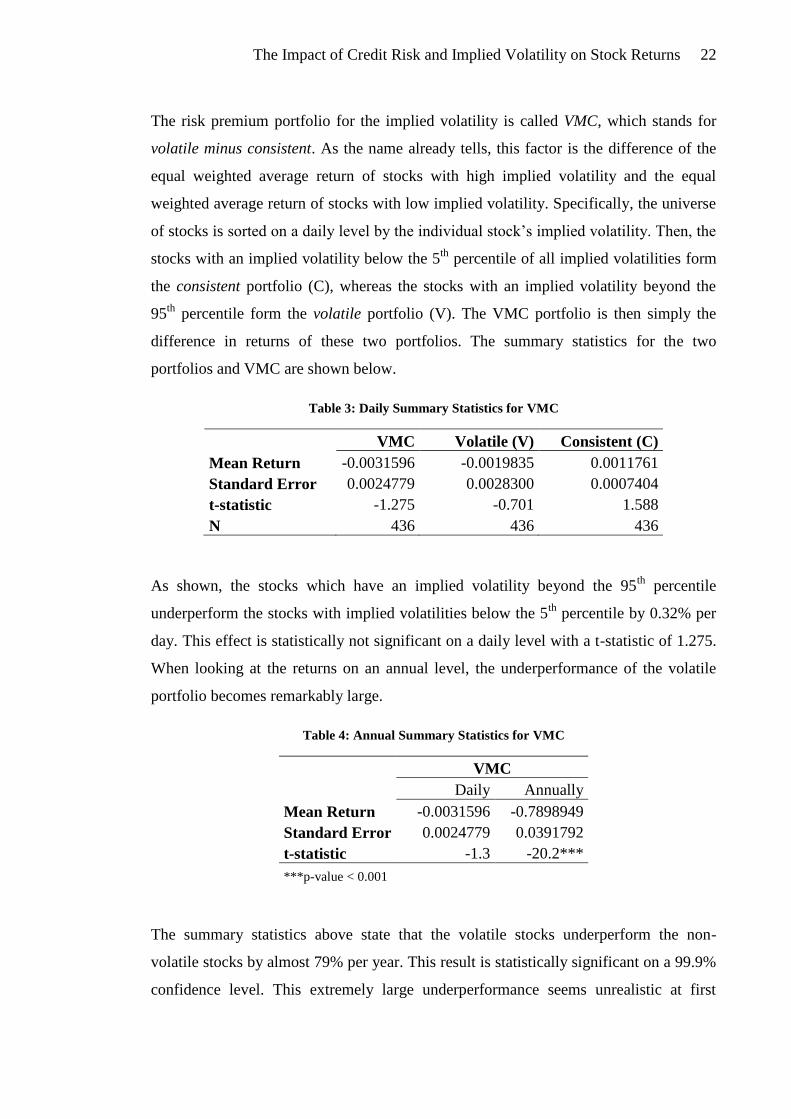
The risk premium portfolio for the implied volatility is called VMC, which stands for
volatile minus consistent. As the name already tells, this factor is the difference of the
equal weighted average return of stocks with high implied volatility and the equal
weighted average return of stocks with low implied volatility. Specifically, the universe
of stocks is sorted on a daily level by the individual stock’s implied volatility. Then, the
stocks with an implied volatility below the 5th
percentile of all implied volatilities form
the consistent portfolio (C), whereas the stocks with an implied volatility beyond the
95th
percentile form the volatile portfolio (V). The VMC portfolio is then simply the
difference in returns of these two portfolios. The summary statistics for the two
portfolios and VMC are shown below.
Table 3: Daily Summary Statistics for VMC
VMC Volatile (V) Consistent (C)
Mean Return -0.0031596 -0.0019835 0.0011761
Standard Error 0.0024779 0.0028300 0.0007404
t-statistic -1.275 -0.701 1.588
N 436 436 436
As shown, the stocks which have an implied volatility beyond the 95th
percentile
underperform the stocks with implied volatilities below the 5th
percentile by 0.32% per
day. This effect is statistically not significant on a daily level with a t-statistic of 1.275.
When looking at the returns on an annual level, the underperformance of the volatile
portfolio becomes remarkably large.
Table 4: Annual Summary Statistics for VMC
VMC
Daily Annually
Mean Return -0.0031596 -0.7898949
Standard Error 0.0024779 0.0391792
t-statistic -1.3 -20.2***
***p-value < 0.001
The summary statistics above state that the volatile stocks underperform the non-
volatile stocks by almost 79% per year. This result is statistically significant on a 99.9%
confidence level. This extremely large underperformance seems unrealistic at first
The Impact of Credit Risk and Implied Volatility on Stock Returns 23
glance and hence further analysis is needed to understand the origins of this remarkable
result.
When looking at the time-series of VMC returns in more detail, it becomes obvious that
the massive underperformance of the volatile stock portfolio is largely driven by the
first 285 days in the sample. During this period, the volatile portfolio underperforms the
consistent portfolio by 0.5% per day. Annualized, this is an underperformance of around
125%. In the subsequent 151 days, that trend changes and the volatile portfolio is being
underperformed by 0.05% a day or 12.5% annually.
Table 5: VMC Time-Series Split
VMC
Until 06/22/09 After 06/22/09
Mean Return -0.0051052 0.0005126
Standard Error 0.0036872 0.0016408
N 285 151
The most probable explanation for this structural break is a sample selection bias. With
an overall number of observations of 436, the sample is very small and includes less
than two years of data. Furthermore, a majority of the data in this sample was collected
in the middle of a massive financial crisis and the external validity of any results based
on this sample should be carefully questioned. The massive underperformance of riskier
stocks shown above could very well be a misleading snapshot that was taken during a
time when massive deleveraging was taking place and investors sold tremendous
amounts of risky assets therefore depressing prices of risky assets. This period was also
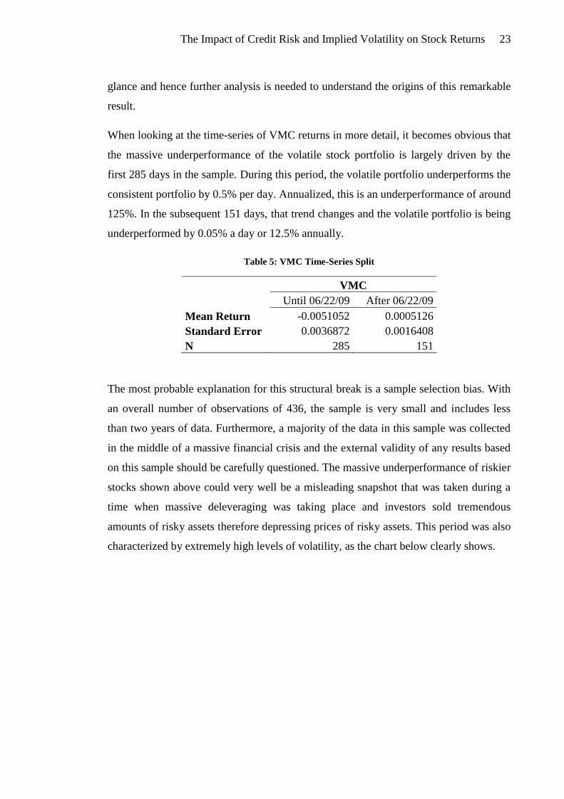
characterized by extremely high levels of volatility, as the chart below clearly shows.

The Impact of Credit Risk and Implied Volatility on Stock Returns 24
Picture 4: VMC Daily Returns
This high level of volatility ends abruptly in June 2009. This timing corresponds to the
time, when the daily underperformance of risky assets transforms into a daily
outperformance of risky assets, as shown above. The most likely explanation for this
behavior is a change in risk appetite by many investors as a result of the financial crisis,
which required investors to massively deleverage. As a consequence of this
deleveraging and the overall reduction in investor’s willingness to take risk, investors
disposed their most risky assets thus depressing share prices of stocks with higher
implied volatility. When this deleveraging and sellout of risk assets ended in June 2009,
investors started to reposition themselves by increasing their overall exposure to risky
assets. As investors increased their positions in these now low-priced assets, the share
prices of these riskier stocks started increasing more than the share prices of stocks with
lower implied volatility.
To conclude: The risk premium for implied volatility is extremely negative. This result
is statistically highly significant on an annual level. However, this result is probably
subject to major sample selection bias since the observation period mainly comprises of
a time period which was characterized by dramatic breaks in market behavior, flights
towards safer assets, and a massive economy-wide deleveraging. Hence, it is evident
-40.00%
-20.00%
0.00%
20.00%
40.00%
Until 06/20/2009 After 06/20/2009

The Impact of Credit Risk and Implied Volatility on Stock Returns 25
that more data, which includes at least one full economic cycle, would be very useful in
increasing the validity of the results presented.
4.4 Regression Analysis
4.4.1 CDS Premium
In order to estimate the factor loadings for the CDS premium factor, the stocks are first
sorted into five quintiles according to the market-to-book (MB) ratio of their equity.
The companies with the lowest MB ratio enter quintile one, the stocks with the highest
MB ratios enter quintile five. For each quintile, the equal weighted average return of the
companies’ stocks is calculated. This procedure is repeated every single trading day.
The basic intuition of sorting the stocks by their MB ratio is to control for the value
effect of stock returns. The value effect states that stocks with lower MB ratios
outperform stocks with higher MB ratios. Fama and French (1998) proposed that this
value effect could actually be a consequence of the fact that companies with low MB
ratios are often distressed companies. If this was true, the regression analysis should
generate higher factor loadings on RMU for lower MB quintiles since distressed
companies usually have higher credit spreads. The five MB quintiles are then regressed
against the risk premium for credit default swap spreads, RMU.
𝑅𝑃 = 𝛼𝑃 + 𝑐𝑃𝑅𝑀𝑈
Table 6: MB Quintiles regressed against RMU
As expected, the factor loadings on RMU are larger for the lower MB quintiles. The
factor loading on RMU for the first quintile is 3.4 times higher than the factor loading of
MB quintile five. Both factor loadings are statistically significant at a 99.9% confidence
level. This decrease in factor loadings supports the above mentioned theory that the
value effect is at least partially a consequence of a credit risk premium earned by
* p<0.05, ** p<0.01, *** p<0.001t statistics in parentheses R-sq 0.771 0.504 0.384 0.343 0.278 N 1304 1304 1304 1304 1304 (-0.85) (0.34) (0.47) (1.10) (1.23) _cons -0.000273 0.000112 0.000141 0.000329 0.000341
(29.64) (18.54) (15.54) (13.76) (10.69) rmu 1.454*** 0.816*** 0.585*** 0.535*** 0.425*** MB Quin~1 2 3 4 MB Quin~5 MB Quintiles regressed against RMU

The Impact of Credit Risk and Implied Volatility on Stock Returns 26
distressed companies’ stocks. In all regressions, the constants are statistically
insignificant.
The R² values also decrease for portfolios with higher MB ratios. The quintile one
portfolio has an R² of above 0.77, whereas the fifth quintile portfolio has an R² of only
0.28. This decrease in the explanatory power of the credit risk premium factor RMU
bears an interesting finding: It seems that the credit risk has a very high explanatory
power for portfolios or stocks with high credit risk, but only a very modest explanatory
power for stocks with lower credit risk. This is an indication that the credit risk of a
specific company has a high influence on the stock price when the company is in
financial distress, but only low influence on companies that are in financially stable
condition. As soon as a company’s financial situation improves, the credit risk is no
longer an important determinant of stock returns. This seems perfectly logical due to
legal and accounting reasons: Credit risk is only important for a shareholder when a
company is in imminent danger of bankruptcy, in which case a shareholder usually
loses his whole investment. If a company is financially stable, the stock return should
theoretically be almost independent of the credit risk. This is very well reflected in the
factor loadings and also the explanatory power; both decrease for companies with less
credit risk.
In order to control for the overall market development, the equal weighted average
return of all stocks in the sample universe (RM) is added to the regression of the five
quintiles.
𝑅𝑃 = 𝛼𝑃 + 𝑐𝑃𝑅𝑀𝑈 + 𝛽𝑃𝑅𝑀
Table 7: MB Quintiles regressed against RMU and RM
* p<0.05, ** p<0.01, *** p<0.001t statistics in parentheses R-sq 0.956 0.948 0.930 0.941 0.920 N 1304 1304 1304 1304 1304 (-2.83) (-0.19) (0.21) (2.30) (2.50) _cons -0.000396** -0.0000204 0.0000210 0.000207* 0.000230*
(49.33) (54.19) (50.00) (74.07) (54.05) rm 1.010*** 1.086*** 0.988*** 1.000*** 0.916***
(24.04) (-0.70) (-9.69) (-16.66) (-17.67) rmu 0.681*** -0.0153 -0.171*** -0.231*** -0.276*** MB Quin~1 2 3 4 MB Quin~5 MB Quintiles regressed against RMU and RM

The Impact of Credit Risk and Implied Volatility on Stock Returns 27
When including the equal weighted average returns of all stocks in this study’s universe
(RM), the factor loadings on RMU decrease but remain statistically significant. The R²
values of the regression increase to values beyond 0.90, thus explaining most of the
variation in stock returns.
As before, the factor loadings on RMU are much higher for the lower MB quintile
stocks than for the high MB quintile stocks. When adding RM as factor to the
regression, an interesting fact becomes evident: The factor loading on RMU is positive
only for the first quintile portfolio but negative for all other quintiles. These loadings are
statistically significant at a 99.9% confidence level, except for the second quintile
portfolio. This is however due to the fact that the factor loadings turn from positive into
negative and hence the factor is not statistically significant different from zero, which is
what the t-statistic measures. This development of the RMU factor loadings, which turn
from positive to negative, is even better visible when looking at the regression with a
higher resolution by dividing the stock universe in deciles instead of quintiles. Please
see table 21 in the appendix for the regression results of MB deciles against RMU and
RM. The development of the factor loadings on RMU of this decile-regression is shown
below:
Picture 5: RMU Factor Loadings of Decile Regression
0.96
0.37
0.00 -0.03-0.15 -0.18 -0.23 -0.23 -0.26 -0.30
0.59
0.37
0.030.12
0.04 0.05 0.01 0.03 0.04
-0.60
-0.40
-0.20
0.00
0.20
0.40
0.60
0.80
1.00
1.20
RMU Factor Loadings Abs. Delta RMU Fctl. Load.

The Impact of Credit Risk and Implied Volatility on Stock Returns 28
As already discovered in the quintile regression, the factor loadings on RMU decrease
for portfolios that have higher MB ratios. The factor loadings are positive for the first
two decile portfolios and eventually turn negative for the other portfolios. These factor
loadings are statistically significant different from zero for most factor loadings except
for the MB deciles in which the factor loadings turn from positive to negative and which
are logically very close zero.
This development of the RMU factor loadings shows that stocks of companies with
higher credit risk earn positive return premiums. The stocks of companies with lower
credit risk earn negative return premiums. It seems that shareholders who bear a higher
amount of default risk are compensated with a stock return premium for bearing that
risk. On the other hand, shareholders who invest in safer stocks with lower credit risk
are receiving a negative return premium. However, the positive return premium for
companies with high credit risk is much higher than the negative return premium for
companies with low credit risk. This is also reflected by a decrease in the absolute
difference in the factor loadings when comparing low quantile portfolios to high
quantile portfolios. The difference in factor loadings from the decile one to decile two is
much higher than the difference from decile nine to decile ten. Graphically, this is
reflected in the diminishing differential of the factor loadings between decile portfolios,
depicted as red line in the above chart. This is an indication that as soon as the credit
risk of a company falls below a certain threshold, it has no influence on stock returns
anymore. In clear words: It does matter if a company’s financial profile changes from
high credit risk to medium credit risk, but changing from low credit risk to extremely
low credit risk has almost no effect on stock returns. This is also underlined by the
development of the R² values for the different quintiles in the regression analysis. The
R² figures decrease for companies with higher MB ratios, implying that the RMU factor
and thus credit risk is less helpful in explaining stock returns for companies with higher
MB ratios or lower credit risk.
From the above presented results it becomes evident that CDS spreads, as proxies for
credit risk, are helpful in explaining stock returns. Companies with higher CDS spreads
tend to have higher stock returns than companies with lower credit risk. This
relationship is stronger for distressed companies, which have low market to book
valuation ratios. The stocks of those distressed companies are earning excess returns for
bearing the risk of default. Stocks of companies with higher MB ratios and thus lower

The Impact of Credit Risk and Implied Volatility on Stock Returns 29
credit risk generate no premium returns; they even earn discounts as a result of the
lower credit risk. This is shown by negative RMU factor loadings for the higher quantile
portfolios when RM is also included in the regression analysis. The explanatory power
of CDS spreads on stock returns decreases for higher market to book ratios, indicating
that the stock returns of companies which are not distressed are less affected by credit
market fluctuations. Once the danger of bankruptcy is not imminent anymore,
shareholders worry about things other than the credit risk of the company. At this point,
other factors such as the corporate strategy and the economic development are more
likely to capture the investors’ attention. This is reflected in declining factor loadings, t-
statistics, and R² for companies with increasing MB ratios. Economically this implies
that credit risk has huge effect on stocks returns only for companies in which the credit
risk is very high. As soon as the credit risk has fallen below a certain level, the
explanatory power of the credit risk premium RMU rapidly deteriorates. Another
interesting finding of this regression is the statistically significant negative intercept for
the quintile 1 portfolio regressed against RM and RMU. Even when controlling for
market return and CDS risk premium, this portfolio generates negative excess return of
roughly 9.9% per year. This intercept is statistically significant on a 99% confidence
level.
4.4.2 Volatility Premium
For the regression estimation of the factor loadings on the volatility premium factor
VMC, the sample size has to be decreased to 436 trading days since data on implied
volatility is only available for a shorter time horizon. The time frame used for this
analysis starts on May 20th
2008 and ends on January 19th
2010. As in the previous
section with the CDS premium factor loadings, a quintile regression is conducted in
which the equal weighted average returns of five portfolios sorted by their MB ratios are
regressed against the VMC and the RM factor. The results of the regression against the
VMC factor alone are shown below:
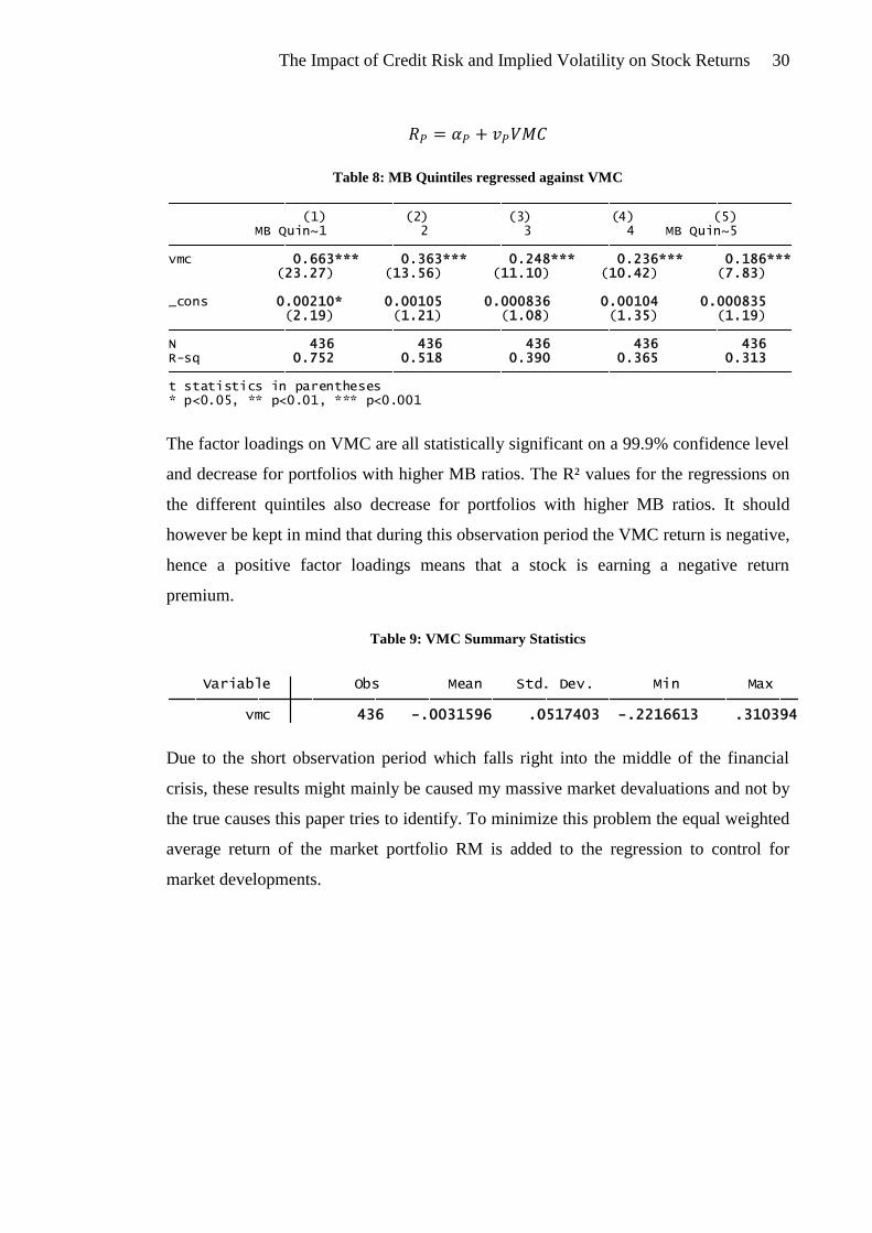
The Impact of Credit Risk and Implied Volatility on Stock Returns 30
𝑅𝑃 = 𝛼𝑃 + 𝑣𝑃𝑉𝑀𝐶
Table 8: MB Quintiles regressed against VMC
The factor loadings on VMC are all statistically significant on a 99.9% confidence level
and decrease for portfolios with higher MB ratios. The R² values for the regressions on
the different quintiles also decrease for portfolios with higher MB ratios. It should
however be kept in mind that during this observation period the VMC return is negative,
hence a positive factor loadings means that a stock is earning a negative return
premium.
Table 9: VMC Summary Statistics
Due to the short observation period which falls right into the middle of the financial
crisis, these results might mainly be caused my massive market devaluations and not by
the true causes this paper tries to identify. To minimize this problem the equal weighted
average return of the market portfolio RM is added to the regression to control for
market developments.
* p<0.05, ** p<0.01, *** p<0.001t statistics in parentheses R-sq 0.752 0.518 0.390 0.365 0.313 N 436 436 436 436 436 (2.19) (1.21) (1.08) (1.35) (1.19) _cons 0.00210* 0.00105 0.000836 0.00104 0.000835
(23.27) (13.56) (11.10) (10.42) (7.83) vmc 0.663*** 0.363*** 0.248*** 0.236*** 0.186*** MB Quin~1 2 3 4 MB Quin~5 (1) (2) (3) (4) (5) MB Quintiles regressed against VMC
vmc 436 -.0031596 .0517403 -.2216613 .310394 Variable Obs Mean Std. Dev. Min Max
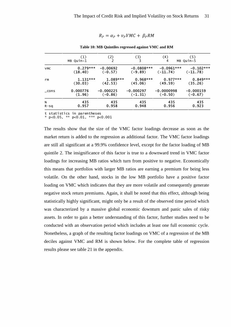
The Impact of Credit Risk and Implied Volatility on Stock Returns 31
𝑅𝑃 = 𝛼𝑃 + 𝑣𝑃𝑉𝑀𝐶 + 𝛽𝑃𝑅𝑀
Table 10: MB Quintiles regressed against VMC and RM
The results show that the size of the VMC factor loadings decrease as soon as the
market return is added to the regression as additional factor. The VMC factor loadings
are still all significant at a 99.9% confidence level, except for the factor loading of MB
quintile 2. The insignificance of this factor is true to a downward trend in VMC factor
loadings for increasing MB ratios which turn from positive to negative. Economically
this means that portfolios with larger MB ratios are earning a premium for being less
volatile. On the other hand, stocks in the low MB portfolio have a positive factor
loading on VMC which indicates that they are more volatile and consequently generate
negative stock return premiums. Again, it shall be noted that this effect, although being
statistically highly significant, might only be a result of the observed time period which
was characterized by a massive global economic downturn and panic sales of risky
assets. In order to gain a better understanding of this factor, further studies need to be
conducted with an observation period which includes at least one full economic cycle.
Nonetheless, a graph of the resulting factor loadings on VMC of a regression of the MB
deciles against VMC and RM is shown below. For the complete table of regression
results please see table 21 in the appendix.
* p<0.05, ** p<0.01, *** p<0.001t statistics in parentheses R-sq 0.957 0.958 0.948 0.956 0.923 N 435 435 435 435 435 (1.96) (-0.86) (-1.31) (-0.50) (-0.67) _cons 0.000776 -0.000225 -0.000297 -0.0000998 -0.000159
(30.03) (42.53) (45.06) (49.59) (35.26) rm 1.131*** 1.089*** 0.968*** 0.977*** 0.849***
(18.40) (-0.57) (-9.89) (-11.74) (-11.78) vmc 0.279*** -0.00692 -0.0808*** -0.0961*** -0.102*** MB Quin~1 2 3 4 MB Quin~5 (1) (2) (3) (4) (5) MB Quintiles regressed against VMC and RM

The Impact of Credit Risk and Implied Volatility on Stock Returns 32
Picture 6: VMC Factor Loadings of Decile Regression
As shown in the graph, the factor loadings are positive for portfolios with low MB
ratios and turn negative for portfolios with higher MB ratios. The rate of change
however rapidly deteriorates as soon as the MB ratios become higher and is
approximately constant for quintiles six to ten. Economically this indicates that stocks
with low MB ratios, which can be seen as distressed stocks, have excess implied
volatility and have consequently earned massive negative premiums in the observed
time period. Stocks with higher MB ratios tended to be less volatile and thus generated
premiums for being less risky assets. However, the premium earned by less volatile
stocks is much smaller than the negative premiums earned by the volatile stocks in the
lowest MB decile.
To conclude this section: Stocks with low MB ratios tend to be more volatile in the
observed time period. During this time period, volatility is highly correlated with
negative returns. Hence, stocks with low MB ratios have underperformed those with
higher MB valuations. As previously discussed, this outcome should be subject to
careful questioning since the observation period is very short and falls into the middle
of the financial crisis. Therefore the result just presented could be biased and its external
validity should be subject of further studies.
0.44
0.10
0.00 -0.01-0.07 -0.09 -0.11 -0.08 -0.10 -0.11
0.34
0.10
0.010.05
0.02 0.02 0.02 0.01 0.01
-0.30
-0.20
-0.10
0.00
0.10
0.20
0.30
0.40
0.50
VMC Factor Loadings Abs. Delta VMC Fctl. Load.

The Impact of Credit Risk and Implied Volatility on Stock Returns 33
4.4.3 CDS-, Volatility-, and Market Premium
As previously discussed, it is evident that the CDS premium factor and the implied
volatility premium factor are helpful in explaining stock returns. In the upcoming
section of this paper, a multifactor model incorporating both of those factors and the
additional market return (RM) is developed. The general equation representing the
return of a stock portfolio which uses these factors as explaining determinants looks as
follows:
𝑅𝑃 = 𝛼𝑃 + 𝑐𝑃 ∙ 𝐶𝐷𝑆 𝑃𝑟𝑒𝑚𝑖𝑢𝑚 + 𝑣𝑃 ∙ 𝑉𝑜𝑙𝑎𝑡𝑖𝑙𝑖𝑡𝑦 𝑃𝑟𝑒𝑚𝑖𝑢𝑚 + 𝛽𝑃 ∙ 𝑀𝑎𝑟𝑘𝑒𝑡 𝑃𝑟𝑒𝑚𝑖𝑢𝑚
Substituting RMU for the CDS premium factor, VMC for the volatility premium factor,
and RM for the market return yields the following regression equation:
𝑅𝑃 = 𝛼𝑃 + 𝑐𝑃 ∙ 𝑅𝑀𝑈 + 𝑣𝑃 ∙ 𝑉𝑀𝐶 + 𝛽𝑃 ∙ 𝑅𝑀
As previously, the equal weighted average returns of the five quintile portfolios sorted
by their market to book ratio (MB) are used as independent variables against which the
three factors are regressed. The portfolio formation methodology is the same as above.
The portfolios are created by sorting the universe into five quintiles according to the
individual stock’s MB ratio. The portfolios are then regenerated every trading day. The
results of regressing the equal weighted average returns of these quintile portfolios
against the three factors are shown below:
Table 11: MB Quintiles regressed against RMU, VMC, and RM
As the above results table indicates, the factor loadings on RMU are positive for quintile
one and turn negative for all higher quintile portfolios. This essentially reflects the same
* p<0.05, ** p<0.01, *** p<0.001t statistics in parentheses R-sq 0.972 0.958 0.950 0.962 0.940 N 435 435 435 435 435 (-0.02) (-0.62) (-0.75) (0.85) (0.90) _cons -0.00000561 -0.000162 -0.000165 0.000154 0.000202
(38.05) (39.79) (41.41) (58.64) (39.00) rm 1.023*** 1.098*** 0.986*** 1.012*** 0.899***
(4.55) (0.36) (-3.78) (-3.55) (-1.71) vmc 0.111*** 0.00652 -0.0523*** -0.0415*** -0.0243
(10.09) (-1.00) (-2.52) (-5.85) (-7.64) rmu 0.493*** -0.0395 -0.0836* -0.161*** -0.228*** MB Quin~1 2 3 4 MB Quin~5 MB Quintiles regressed against RMU, VMC, and RM
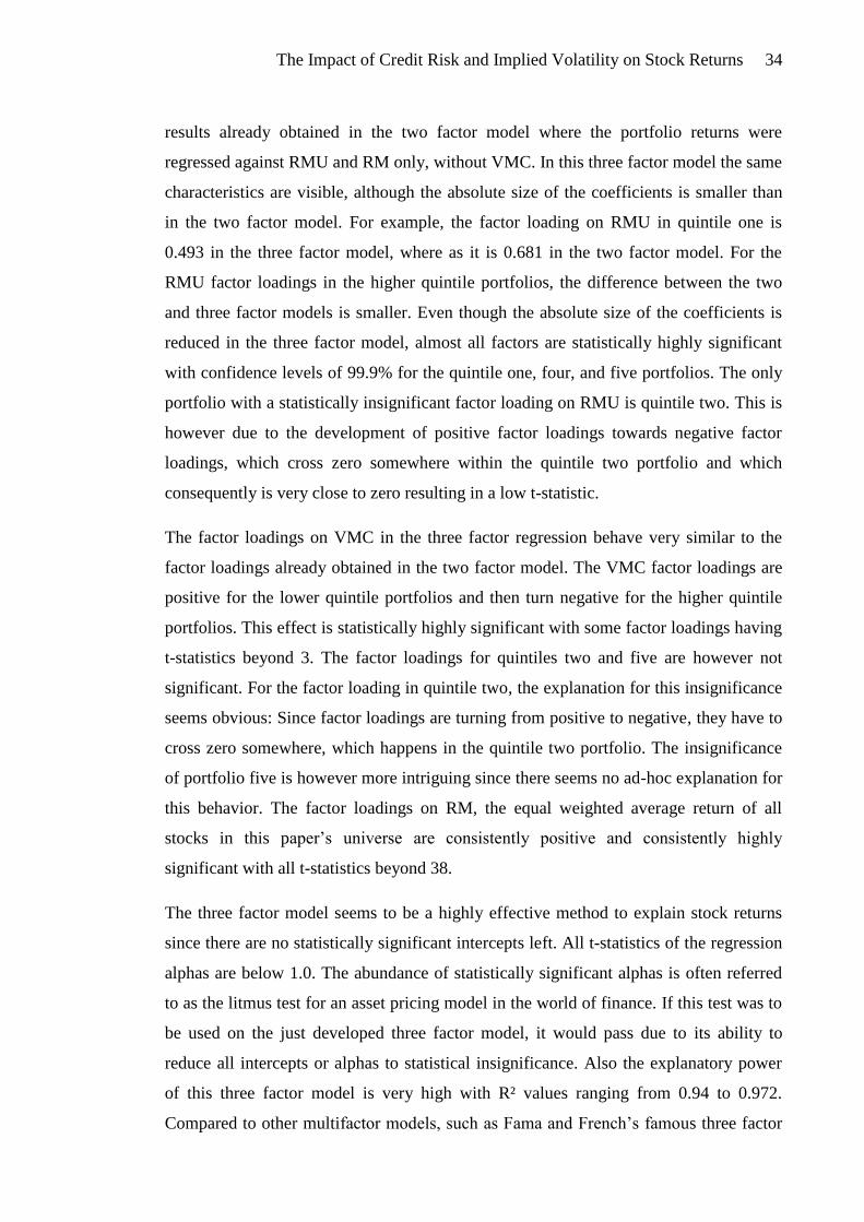
The Impact of Credit Risk and Implied Volatility on Stock Returns 34
results already obtained in the two factor model where the portfolio returns were
regressed against RMU and RM only, without VMC. In this three factor model the same
characteristics are visible, although the absolute size of the coefficients is smaller than
in the two factor model. For example, the factor loading on RMU in quintile one is
0.493 in the three factor model, where as it is 0.681 in the two factor model. For the
RMU factor loadings in the higher quintile portfolios, the difference between the two
and three factor models is smaller. Even though the absolute size of the coefficients is
reduced in the three factor model, almost all factors are statistically highly significant
with confidence levels of 99.9% for the quintile one, four, and five portfolios. The only
portfolio with a statistically insignificant factor loading on RMU is quintile two. This is
however due to the development of positive factor loadings towards negative factor
loadings, which cross zero somewhere within the quintile two portfolio and which
consequently is very close to zero resulting in a low t-statistic.
The factor loadings on VMC in the three factor regression behave very similar to the
factor loadings already obtained in the two factor model. The VMC factor loadings are
positive for the lower quintile portfolios and then turn negative for the higher quintile
portfolios. This effect is statistically highly significant with some factor loadings having
t-statistics beyond 3. The factor loadings for quintiles two and five are however not
significant. For the factor loading in quintile two, the explanation for this insignificance
seems obvious: Since factor loadings are turning from positive to negative, they have to
cross zero somewhere, which happens in the quintile two portfolio. The insignificance
of portfolio five is however more intriguing since there seems no ad-hoc explanation for
this behavior. The factor loadings on RM, the equal weighted average return of all
stocks in this paper’s universe are consistently positive and consistently highly
significant with all t-statistics beyond 38.
The three factor model seems to be a highly effective method to explain stock returns
since there are no statistically significant intercepts left. All t-statistics of the regression
alphas are below 1.0. The abundance of statistically significant alphas is often referred
to as the litmus test for an asset pricing model in the world of finance. If this test was to
be used on the just developed three factor model, it would pass due to its ability to
reduce all intercepts or alphas to statistical insignificance. Also the explanatory power
of this three factor model is very high with R² values ranging from 0.94 to 0.972.
Compared to other multifactor models, such as Fama and French’s famous three factor

The Impact of Credit Risk and Implied Volatility on Stock Returns 35
model (1993), which results in R² values between 0.93 and 0.94, the three factor model
proposed in this paper seems to be doing quite a good job to explain stock returns. A
regression of the MB quintiles against the original Fama-French factors HML and SMB
(French K. , 2010) as well as RM is shown below.
Table 12: MB Quintiles regressed against HML, SMB, and RM
Due to the fact that the Fama-French factors are not available for the last recent months,
the sample size is reduced to 367 trading days. As shown above, the factor loading on
HML is highly significant and shows a similar behavior as the RMU factor: It starts off
with a positive coefficient which then turns negative for all quintile portfolios beyond
one. The factor loadings on SMB are almost all statistically non significant, which
seems logical since there are only large-cap stocks included in this paper’s sample.
Although the HML and the RMU factors are highly correlated with a correlation
coefficient of 0.80, they still seem to measure different things. A regression including
both has statistically significant positive factor loadings on both factors as table 24 in
the appendix shows. The only possible explanation for such a high significance and
high correlation other than a true causal difference would be a similar trend in both time
series which is picked up by the OLS estimation. However, as a Dickey-Fuller test
reveals (see table 25 in the appendix), RMU and HML are stationary and hence it is
evident that even though both factors are highly correlated, they still measure different
effects at least to a certain extent.
Apart from the original task to develop a working multifactor model based on derivative
implied factors, the three factor model based on RMU, VMC, and RM also generates an
* p<0.05, ** p<0.01, *** p<0.001t statistics in parentheses R-sq 0.944 0.959 0.938 0.950 0.929 N 367 367 367 367 367 (-0.22) (-0.67) (-0.15) (0.49) (0.95) _cons -0.000119 -0.000201 -0.0000431 0.000125 0.000248
(25.69) (50.03) (29.10) (38.66) (43.15) rm 1.314*** 1.086*** 0.899*** 0.916*** 0.795***
(-0.67) (-1.64) (2.13) (1.58) (-0.94) smb -0.0504 -0.0808 0.0988* 0.0616 -0.0300
(10.72) (-0.99) (-3.71) (-7.68) (-11.19) hml 0.957*** -0.0422 -0.196*** -0.328*** -0.410*** MB Quin~1 2 3 4 MB Quin~5 MB Quintiles regressed against HML, SMB, and RM

The Impact of Credit Risk and Implied Volatility on Stock Returns 36
interesting insight on the often discussed value effect of stock returns which states that
stocks with lower MB ratios outperform stocks with higher MB ratios.
When looking at the factor loadings on RMU and VMC, it becomes evident that the
findings of the isolated regressions still hold for the complete factor model. Stocks with
low MB ratios tend to have positive factor loadings on RMU as well as VMC, whereas
stocks with higher MB ratios lean towards negative factor loadings. The chart below
shows the development of the factor loadings on RMU and VMC derived from a decile
regression which also included RM. The full table of results of this regression can be
seen in table 11 in the appendix.
Picture 7: RMU and VMC Factor Loadings of Decile Regression
As shown, the factor loadings on both factors are positive for the first decile and turn
negative for most of the higher decile portfolios. Also the absolute size of the factor
loadings rapidly deteriorates. Especially the VMC factor loadings seem to
asymptotically approach zero in the higher decile portfolios, where they are not even
statistically different from zero anymore. This implies that the implied volatility
premium, which during this observation period was negative, leads to high negative
effects on stocks with low MB ratios but only to small positive effects on stocks with
high MB ratios. It seems that the implied volatility is a more important topic for
distressed securities than it is for securities with higher MB valuations. A similar logic
-0.30
-0.20
-0.10
0.00
0.10
0.20
0.30
0.40
0.50
0.60
RMU Factor Loadings VMC Factor Loadings
The Impact of Credit Risk and Implied Volatility on Stock Returns 37
holds true for the RMU factor. Stocks within the lower MB decile portfolios tend to
have higher credit spreads as a result of a higher risk of default. Shareholders are
compensated for bearing this risk of default by higher stock returns. As soon as the
company’s credit risk and MB ratio improve, the positive premium earned for bearing
credit risk first becomes zero and later even turns negative. The rate of change also
massively deteriorates for higher decile portfolios. This means that credit risk is a huge
topic for stocks in the lowest MB deciles, but only a minor topic for all other deciles.
These effects lead to the outperformance of low MB stocks compared to high MB
stocks, commonly known as the value effect.
To conclude: The development of the RMU and VMC factor loadings allows
decomposing the value effect into a credit risk premium and a volatility risk premium.
Stocks with lower MB ratios have positive factor loadings on RMU and VMC. This
means that they are earning a positive return premium for bearing credit risk and a
negative return premium for bearing volatility risk. This negative volatility risk
premium is however subject to a sample selection bias, which includes a time horizon
which is too short to draw any significant conclusions. The findings and implications of
the factor loadings on the credit risk premium are more robust since they were
essentially the same during the five year observation period.
5 Summary
5.1 Discussion of Results
The determination of the factor premia has shown that stocks with higher CDS spreads
tend to earn a premium over the stocks with lower CDS spreads. Considering classic
capital market theories this also seems logical since investors who bear higher risks
have to be compensated with higher returns for bearing that risk. During the observation
period, the stocks whose CDS spreads were above the 75th
percentile outperformed the
stocks whose CDS spreads were below the 25th
percentile by 5.89% on an annual level.
This effect is statistically significant with an extrapolated t-statistic of 9.2 on an annual
level.
For the implied volatility the contrary is true. Stocks whose implied volatility is beyond
the 95th
percentile underperformed stocks whose implied volatility is below the 5th
percentile by roughly 79% per year during the observed period. The validity of this
The Impact of Credit Risk and Implied Volatility on Stock Returns 38
finding is however very limited since the observation period for the implied volatilities
in this paper is rather short and falls right within the middle of the global financial
crisis, during which investors tried to dispose their risky assets, therefore plummeting
share prices of stocks with higher implied volatilities. When splitting the observation
period into two parts, it becomes evident that during the first 285 observation days the
relationship between return and implied volatility was negative but that it was positive
for the following 151 observations. This is evidence for a structural break of the risk-
return relationship within this time-series which further indicates the necessity of using
a larger observation period to confirm the validity of the results obtained in this paper.
If this paper’s results were valid, they would violate the classic assumption that a higher
expected risk should be rewarded by higher expected returns.
The results obtained through regressing the equal weighted average stock returns of
various portfolios, which have been formed through sorting the stocks by their MB
ratio, have shown that the CDS premium factor, called RMU, is helpful in explaining
stock returns. However, the explanatory power and the size of the factor loadings on
RMU tend to decrease for portfolios with higher MB ratios. When the MB ratio is seen
as an indicator for distress, this leads to an interesting finding. The rapid deterioration of
the R² and the factor loadings on RMU reflects the fact that credit risk is only important
to shareholders when it is very high. As soon as the credit risk gets lower and the MB
ratios correspondingly increase, credit risk becomes almost irrelevant to investors. It
also becomes evident that the so-called value effect is not an anomaly in market
behavior but actually a logical consequence of credit risk. Stock holders bearing a risk
of losing their whole investment in the case of a credit event are being compensated for
that risk. This risk premium does, at least partially, explain the value effect of stock
returns. It is further very interesting to see that this effect is almost entirely created by
the lowest quintile or decile portfolios, which account for a majority of the difference in
returns. This is reflected in high positive factor loadings for low MB quintile stocks but
only slightly negative factor loadings for high MB quintile stocks.
The regression analyses on the VMC factor, which controls for the implied volatilities,
have shown that stocks with low MB ratios tend to have more implied volatility
compared to the market average. Since above average implied volatility was rewarded
with negative return premiums during the observed time period, the stocks in the low
MB quintile portfolios earn negative return premiums compared to stocks with higher

The Impact of Credit Risk and Implied Volatility on Stock Returns 39
MB ratios which have less implied volatility. The factor loadings on VMC are
especially high for the lower MB decile or quintile portfolios and turn negative for the
higher portfolios. The absolute size of the factor loadings is also much higher for stocks
with lower MB ratios. This is evidence that the implied volatility is a more important
determinant of stock returns for stocks with high implied volatility than for stocks with
low volatility. This means that stock returns are largely affected by high implied
volatilities in the low MB sector, but that low volatilities on the other hand have only
minor effects on stock returns.
In the full three factor regression model, which includes both derivative implied factors
(RMU and VMC) as well as the market return (RM), it becomes evident that the CDS
spread as well as the implied volatility are indeed helpful in explaining stock returns.
Most of the factor loadings on the explaining factors are statistically highly significant,
except for those quintiles in which the factor loadings turn from positive into negative
territory. The positive factor loadings on RMU and VMC in the lower MB portfolios
show that low MB ratios are correlated with higher credit spreads and higher implied
volatilities. For stocks with higher MB ratios these factor loadings decrease and become
even negative for stocks with the highest MB ratios. This indicates that low MB stocks
earn a premium for higher credit risk and a discount for higher implied volatility. As the
MB ratio increases, the credit spreads and implied volatility decrease and so do the
factor loadings on the RMU and VMC factors. The interesting fact is not that the factor
loadings turn from positive to negative, but that the absolute value of the factor loadings
for lower MB stocks is much higher than the absolute value for higher MB stocks. This
shows that credit risk and volatility are more important determinants of a stock’s return
when the credit risk and implied volatility are high, than for stocks with lower risks. It
seems that as soon as company’s credit risk and its stock’s implied volatility have fallen
below a certain threshold, these two variables lose a large portion of their explanatory
power. Especially for credit risk this finding makes sense since the risk of default is
only relevant for a shareholder if there is a high probability that a company defaults in
which case the shareholder would lose his investment. If the credit risk is already on a
very low level, shareholders focus their attention on topics other than credit risk.
Also the explanatory power of this three factor model is very high with R² values
between 0.94 and 0.97 in the quintile regression analysis. This is even slightly higher
than the R² values achieved in the Fama-French three factor analysis. Also the fact that
The Impact of Credit Risk and Implied Volatility on Stock Returns 40
all intercepts, also often referred to as alphas, are statistically insignificant. This
insignificance in combination with the high explanatory power which explains almost
all variation in stock returns underlines the usefulness of this multifactor model based
on derivative data. It seems that the credit default swap spreads as well as the implied
volatility are useful factors in explaining stock returns.
In addition to the finding that the three factor model is useful for explaining stock
returns, this paper also makes interesting findings regarding the value effect of stock
returns by observing the development of the factor loadings in relationship to the MB
ratio. The different factor loadings on RMU and VMC for the specific MB portfolios
show that the value effect could, at least partially, be attributed to a credit risk premium
and possibly an implied volatility premium. Stocks with lower MB ratios bear excess
credit risk which is being compensated by a positive premium on stock returns. This
positive premium for low MB stocks is larger than the negative premium earned by high
MB stocks. Hence, the value effect is not an anomaly of capital markets but adequately
expresses a positive return premium for credit risk which is inflicted upon an investor of
low MB stocks. It is likely that a similar conclusion could be drawn for the implied
volatility, but due to the already discussed sample bias which includes a too short time
horizon, a larger sample is needed for further analysis.
The findings of this paper also have some practical implications. The possibility to
explain stock returns through credit market derivatives could potentially allow for cross-
hedging the exposures of these different asset classes. Especially a long exposure in
stocks with high credit risk could be partially hedged through a replication of the RMU
portfolio or a direct investment in CDS. The econometric regression model shown
above could be modified in order to calculate the exact hedge ratios needed for an
optimal hedge. The presented relationship between the stock and the credit market
would also allow improving risk assessment systems through incorporating possible
correlation and cluster risks which affect stock as well as credit markets.
Another advantage of the proposed three factor model is that the credit risk and the
implied volatility are very sluggish and can hence be predicted very accurately over a
short-term horizon. The possibility of predicting these two factors could theoretically
allow creating profitable trading strategies based on the RMU and VMC portfolio.

The Impact of Credit Risk and Implied Volatility on Stock Returns 41
5.2 Ideas for Further Research
Especially the small observation period for the implied volatility factor is a problem that
should be avoided in further studies. In order to make accurate and reliable statements
about the relationship between stock returns and the implied volatility, a larger sample
size is needed. If possible, the time horizon should include several full economic cycles
and thus be at least 10 years long. The only limitation to the time horizon is the
availability of data on credit default swaps and equity options, which are used to
calculate the implied volatility.
Additionally, further studies should not only try to use a longer time period but also to
include a larger stock universe. Using a larger universe would allow to include more
risk factors such as the size of a company in the regression analysis. Since all S&P 100
stocks used as universe in this paper are large-cap stocks, size effects are virtually not
analyzable by using the universe of in this paper. By including additional stocks, it
would be very interesting to analyze the factor loadings on RMU and VMC of
portfolios which have been created with size or market cap as sorting criteria instead of
the market to book ratio. A disadvantage however of using a larger universe is the fact
that the availability and liquidity of derivatives is much smaller for small-cap stocks
than it is for large-cap stocks.
Another potential idea for research would be to decompose the Fama-French HML
factor, also known as value factor, into credit risk and implied volatility risk. If the
conclusion of this paper is correct, it should be possible to explain a large portion of this
HML factor through credit risk and implied volatility. Also a comparison of the three
factor model developed in this paper and its replication using cash market bond spreads
instead of CDS spreads would be interesting to conduct. In terms of the econometric
methods used, a cross-sectional test of the results presented in this paper analogue to the
procedure used by Black, Jensen, and Scholes (1972) could reveal further insights.
5.3 Conclusion
This paper has shown that derivative markets can be used to build multifactor asset
pricing models. The CDS spread and the implied volatility of a stock are helpful
determinants in explaining the return behavior of stocks. Especially stocks with high
credit risk and high implied volatility are largely affected by the premiums earned on
these two factors. Stocks with low credit risk and low implied volatility are almost

The Impact of Credit Risk and Implied Volatility on Stock Returns 42
unaffected by these two factors. Since credit risk and volatility are correlated with the
market to book ratio of a stock, it can be concluded that the often discussed value effect
is not an effect of a market anomaly or irrational investing behavior: The value effect is
actually a consequence of the credit risk and the implied volatility of a company. If a
company has a low MB ratio, its credit risk and its implied volatility are very high and
the shareholder is in imminent danger of losing his investment. That risk is being
rewarded with positive stock return premiums. As soon as the MB ratio and with it the
credit risk and the implied volatility improve, the factor loadings on the risk premia
largely disappear. As soon as a certain threshold is passed, investors stop worrying
about credit risk and implied volatility and probably focus their attention on different
aspects, such as corporate strategy and the overall economic development.
It can therefore be concluded that the model developed in this paper is a useful
expansion of previously developed multifactor models. The high statistical significance
of the factor loadings and the large overall explanatory power of the proposed three
factor model based on market return, credit default swap spreads, and implied volatility
make it clear that derivative markets are very useful in developing asset pricing models
and estimating risk premia.

The Impact of Credit Risk and Implied Volatility on Stock Returns 43
Bibliography
Black, F., & Scholes, M. (1973). The Pricing of Options and Corporate Liabilities. The
Journal of Political Economy , 637-654.
Black, F., Jensen, M. C., & Scholes, M. (1972). The Capital Asset Pricing Model: Some
Empirical Tests. Studies in the Theory of Capital Markets , 79–121.
Campbell, J. Y., & Hentschel, L. (1992). No News is Good News - An Asymmetric
Model of Changing Volatility in Stock Returns. Journal of Financial Economics
, 281-318.
Campbell, J. Y., & Shiller, R. J. (1988). Stock Prices, Earnings, and Expected
Dividends. The Journal of Finance , 661-676.
Carhart, M. M. (1997). On Persistence in Mutual Fund Performance. The Journal of
Finance , 57-82.
Carr, P., & Wu, L. (2009). Stock Options and Credit Default Swaps: A Joint Framework
for Valuation and Estimation. Journal of Financial Econometrics , 1-41.
Chen, N.-F., Roll, R., & Ross, S. A. (1986). Economic Forces and the Stock Market.
The Journal of Business , 383-403.
Cox, J. C., Ingersoll, J. E., & Ross, S. A. (1985). An Intertemporal General Equilibrium
Model of Asset Prices. Econometrica , 363-384.
Daniels, K. N., & Jensen, M. S. (2005). The Effect of Credit Ratings on Credit Default
Swap Spreads and Credit Spreads. Journal of Fixed Income , 16-33.
DeBondt, W. F., & Thaler, R. (1985). Does the Stock Market Overreact? The Journal of
Finance , 793-805.
DeLong, J. B., Shleifer, A., Summers, L. H., & Waldman, R. J. (1990). Positive
Feedback Investment Strategies and Destabilizing Rational Speculation. The
Journal of Finance , 379-395.
Derman, E., & Kani, I. (1994). Riding on a Smile. Risk , 32-39.
Dupire, B. (1994). Pricing with a Smile. Risk , 18-20.
The Impact of Credit Risk and Implied Volatility on Stock Returns 44
European Central Bank. (2009). Credit Default Swaps and Counterparty Risk.
Frankfurt: European Central Bank.
Fabozzi, F. J. (2005). The Handbook of Fixed Income Securities. New York: McGraw-
Hill.
Fama, E. F., & French, K. R. (1989). Business Conditions and Expected Returns on
Stocks and Bonds. Journal of Financial Economics , 23-49.
Fama, E. F., & French, K. R. (1993). Common Risk Factors in the Returns of Stocks
and Bonds. Journal of Financial Economics , 3-56.
Fama, E. F., & French, K. R. (1992). The Cross-Section of Expected Stock Returns. The
Journal of Finance , 427-465.
Fama, E. F., & French, K. R. (1998). Value Versus Growth: The International Evidence.
The Journal of Finance , 1975-1999.
French, K. (2010, January 1). Fama French Factors. Retrieved January 1, 2010, from
http://mba.tuck.dartmouth.edu/pages/faculty/ken.french/data_library.html
French, K. R., Schwert, G. W., & Stambaugh, R. F. (1986). Expected Stock Returns and
Volatility. Journal of Financial Economics , 3-29.
Glosten, L. R., Jagannathan, R., & Runkle, D. E. (1993). On the Relation between the
Expected Value and the Volatility of the Nominal Excess Return on Stocks. The
Journal of Finance , 1779-1801.
Hull, J. C. (2009). Options, Futures, and Other Derivatives. New Jersey: Pearson
Prentice Hall.
International Swaps and Derivatives Association. (2010, January 12). ISDA CDS
Master Agreement. New York, NY, United States of America: ISDA. Retrieved
from ISDA CDS Master Agreement: http://www.isda.org/cgi-
bin/_isdadocsdownload/download.asp?DownloadID=84
Jegadeesh, N., & Titman, S. (1993). Returns to Buying Winners and Selling Losers:
Implications for Stock Market Efficiency. The Journal of Finance , 65-91.

The Impact of Credit Risk and Implied Volatility on Stock Returns 45
Jones, C. M., & Lamont, O. A. (2002). Short-Sale Constraints and Stock Returns.
Journal of Financial Economics , 207-239.
Kawaller, I. G., Koch, P. D., & Koch, T. W. (1987). The Temporal Price Relationship
between S&P 500 Futures and the S&P 500 Index. The Journal of Finance ,
1309-1329.
Lamont, O. (1998). Earnings and Expected Returns. The Journal of Finance , 1563-
1587.
Lintner, J. (1965). The Valuation of Risk Assets and the Selection of Risky Investments
in Stock. The Review of Economics and Statistics , 13-37.
Longstaff, F. A., & Schwartz, E. S. (2001). Valuing American Options by Simulation:
A Simple Least-Squares Approach. The Review of Financial Studies , 113-147.
Markowitz, H. (1952). Portfolio Selection. The Journal of Finance , 77-91.
Merton, R. C. (1973). An Intertemporal Capital Asset Pricing Model. Econometrica ,
867-887.
Merton, R. C. (1973). Theory of Rational Option Pricing. The Bell Journal of
Economics and Management Science , 141-183.
Norden, L., & Weber, M. (2009). The Co-movement of Credit Default Swap, Bond, and
Stock Markets: An Empirical Analysis. European Financial Management , 529-
562.
Ross, S. A. (1976). The Arbitrage Theory of Capital Asset Pricing. Journal of Economic
Theory , 341-360.
Rubinstein, M. (1994). Implied Binomial Trees. The Journal of Finance , 771-818.
Sharpe, W. F. (1964). Capital Asset Prices: A Theory of Market Equillibrium Under
Conditions of Risk. The Journal of Finance , 425-442.
Sharpe, W. F. (1966). Mutual Fund Performance. Journal of Business , 119-138.
Sortino, F., & Van der Meer, R. (1991). Downside Risk. The Journal of Portfolio
Management , 27-31.

The Impact of Credit Risk and Implied Volatility on Stock Returns 46
US Securities and Exchange Commission. (2008, September 23th). Testimony
Concerning Turmoil in U.S. Credit Markets: Recent Actions Regarding
Government Sponsored Entities, Investment Banks and Other Financial
Institutions. Retrieved January 4th, 2010, from US Securities and Exchange
Commission: http://www.sec.gov/news/testimony/2008/ts092308cc.htm
Zhang, B. Y., Zhou, H., & Zhu, H. (2009). Explaining Credit Default Swap Spreads
with the Equity Volatility and Jump Risks of Individual Firms. The Review of
Financial Studies , 5099-5131.

The Impact of Credit Risk and Implied Volatility on Stock Returns 47
Appendix
Table 13: Risk Factors (Chen, Roll, & Ross, 1986)
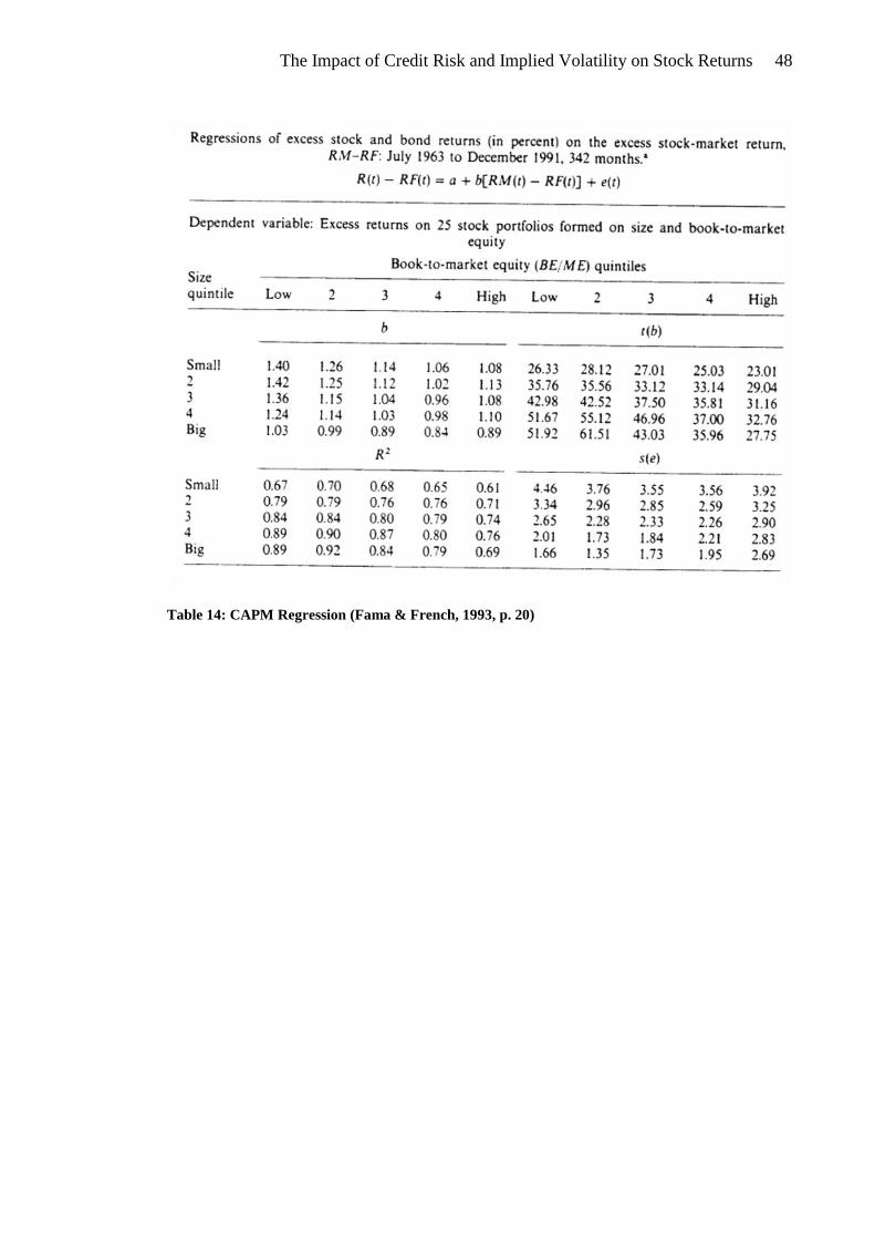
The Impact of Credit Risk and Implied Volatility on Stock Returns 48
Table 14: CAPM Regression (Fama & French, 1993, p. 20)
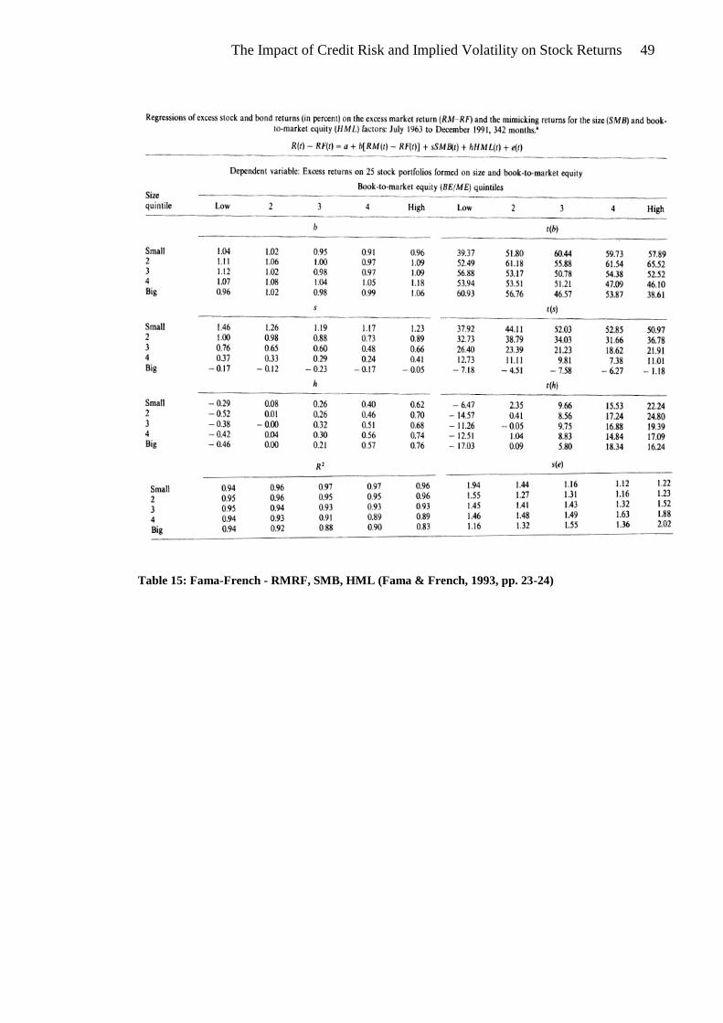
The Impact of Credit Risk and Implied Volatility on Stock Returns 49
Table 15: Fama-French - RMRF, SMB, HML (Fama & French, 1993, pp. 23-24)

The Impact of Credit Risk and Implied Volatility on Stock Returns 50
Table 16: Fama-French - TERM, DEF (Fama & French, 1993, p. 17)

The Impact of Credit Risk and Implied Volatility on Stock Returns 51
Table 17: Fama-French - RMRF, SML, HML, TERM, DEF (Fama & French, 1993, pp. 28-29)

The Impact of Credit Risk and Implied Volatility on Stock Returns 52
Table 18: Carhart - Summary Statistics (Carhart, 1997, p. 77)

The Impact of Credit Risk and Implied Volatility on Stock Returns 53
Table 19: Carhart - Factor Loadings (Carhart, 1997, p. 64)
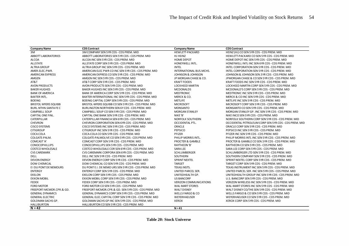
The Impact of Credit Risk and Implied Volatility on Stock Returns 54
Table 20: Stock Universe
Company Name CDS Contract Company Name CDS Contract3M 3M COMPANY SEN 5YR CDS - CDS PREM. MID HEWLETT-PACKARD HEINZ (HJ) CO SEN 5YR CDS - CDS PREM. MIDABBOTT LABORATORIES ABBOTT LABORATORIES SEN 5YR CDS - CDS PREM. MID HJ HEINZ HEWLETT-PACKARD CO SEN 5YR CDS - CDS PREM. MIDALCOA ALCOA INC SEN 5YR CDS - CDS PREM. MID HOME DEPOT HOME DEPOT INC SEN 5YR CDS - CDS PREM. MIDALLSTATE ALLSTATE CORP SEN 5YR CDS - CDS PREM. MID HONEYWELL INTL. HONEYWELL INTL INC SEN 6YR CDS - CDS PREM. MIDALTRIA GROUP ALTRIA GROUP INC SEN 5YR CDS - CDS PREM. MID INTEL INTEL CORPORATION SEN 5YR CDS - CDS PREM. MIDAMER.ELEC.PWR. AMERICAN ELEC PWR CO INC SEN 5YR CDS - CDS PREM. MID INTERNATIONAL BUS.MCHS. INTEL CORPORATION SEN 5YR CDS - CDS PREM. MIDAMERICAN EXPRESS AMERICAN EXPRESS CO SEN 5YR CDS - CDS PREM. MID JOHNSON & JOHNSON JOHNSON & JOHNSON SEN.5YR CDS - CDS PREM. MIDAMGEN AMGEN INC SEN 5YR CDS - CDS PREM. MID JP MORGAN CHASE & CO. JPMORGAN CHASE & CO SEN 5YR CDS - CDS PREM. MIDAT&T AT&T CORP SEN 5YR CDS - CDS PREM. MID KRAFT FOODS KRAFT FOODS INC SEN 5YR CDS - CDS PREM. MIDAVON PRODUCTS AVON PRODUCTS SEN 5YR CDS - CDS PREM. MID LOCKHEED MARTIN LOCKHEED MARTIN CORP SEN 5YR CDS - CDS PREM. MIDBAKER HUGHES BAKER HUGHES INC SEN 5YR CDS - CDS PREM. MID MCDONALDS MCDONALD'S CORP SEN 5YR CDS - CDS PREM. MIDBANK OF AMERICA BANK OF AMERICA CORP SEN 5YR CDS - CDS PREM. MID MEDTRONIC MEDTRONIC INC SEN 5YR CDS - CDS PREM. MIDBAXTER INTL. BAXTER INTERNATIONAL INC SEN 5YR CDS - CDS PREM. MID MERCK & CO. MERCK & CO INC SEN 5YR CDS - CDS PREM. MIDBOEING BOEING CAPITAL CORP SEN 5YR CDS - CDS PREM. MID METLIFE METLIFE INC SEN 5YR CDS - CDS PREM. MIDBRISTOL MYERS SQUIBB BRISTOL-MYERS SQUIBB CO SEN 5YR CDS - CDS PREM. MID MICROSOFT MICROSOFT CORP SEN 5YR CDS - CDS PREM. MIDBURL.NTHN.SANTA FE C BURLINGTON NORTHERN SEN 6Y CDS - CDS PREM. MID MONSANTO MONSANTO CO SEN 5YR CDS - CDS PREM. MIDCAMPBELL SOUP CAMPBELL SOUP CO SEN 5YR CDS - CDS PREM. MID MORGAN STANLEY MORGAN STANLEY GP. INC SEN 5YR CDS - CDS PREM. MIDCAPITAL ONE FINL. CAPITAL ONE BANK SEN 5YR CDS - CDS PREM. MID NIKE 'B' NIKE INCO SEN 5YR CDS - CDS PREM. MIDCATERPILLAR CATERPILLAR FINANCIA SEN 6YR CDS - CDS PREM. MID NORFOLK SOUTHERN NORFOLK SOUTHERN CORP SEN 5YR CDS - CDS PREM. MIDCHEVRON CHEVRON CORPORATION SEN 6YR CDS - CDS PREM. MID OCCIDENTAL PTL. OCCIDENTAL PETROLEUM CORP SEN 5YR CDS - CDS PREM. MIDCISCO SYSTEMS CISCO SYSTEMS INC SEN 5YR CDS - CDS PREM. MID ORACLE ORACLE CORP SEN 5YR CDS - CDS PREM. MIDCITIGROUP CITIGROUP INC SEN 5YR CDS - CDS PREM. MID PEPSICO PEPSICO INC SEN 5YR CDS - CDS PREM. MIDCOCA COLA COCA-COLA CO SEN 5YR CDS - CDS PREM. MID PFIZER PFIZER INC SEN 5YR CDS - CDS PREM. MIDCOLGATE-PALM. COLGATE-PALMOLIVE CO SEN 5YR CDS - CDS PREM. MID PHILIP MORRIS INTL. PHILIP MORRIS INTL INC SEN 5YR CDS - CDS PREM. MIDCOMCAST 'A' COMCAST CORP SEN 5YR CDS - CDS PREM. MID PROCTER & GAMBLE PROCTER & GAMBLE CO SEN.5YR CDS - CDS PREM. MIDCONOCOPHILLIPS CONOCOPHILLIPS SEN 5YR CDS - CDS PREM. MID RAYTHEON 'B' RAYTHEON CO SEN 5YR CDS - CDS PREM. MIDCOSTCO WHOLESALE COSTCO WHOLESALE COR SEN 6YR CDS - CDS PREM. MID SARA LEE SARA LEE CORP SEN 5YR CDS - CDS PREM. MIDCVS CAREMARK CVS CAREMARK CORPORA SEN 6YR CDS - CDS PREM. MID SCHLUMBERGER SCHLUMBERGER LTD SEN 5YR CDS - CDS PREM. MIDDELL DELL INC SEN 5YR CDS - CDS PREM. MID SOUTHERN SOUTHERN COMPANY SEN 5YR CDS - CDS PREM. MIDDEVON ENERGY DEVON ENERGY CORP SEN 5YR CDS - CDS PREM. MID SPRINT NEXTEL SPRINT NEXTEL CORP SEN 5YR CDS - CDS PREM. MIDDOW CHEMICAL DOW CHEMICAL CO SEN 5YR CDS - CDS PREM. MID TARGET TARGET CORP SEN 5YR CDS - CDS PREM. MIDE I DU PONT DE NEMOURS DU PONT E.I. DE NEMO URS SEN 5YR CDS - CDS PREM. MID TEXAS INSTS. TEXAS INSTRUMENT INC SEN 5YR CDS - CDS PREM. MIDENTERGY ENTERGY CORP SEN 5YR CDS - CDS PREM. MID UNITED PARCEL SER. UNITED PARCEL SER. INC SEN 5YR CDS - CDS PREM. MIDEXELON EXELON CORP SEN 5YR CDS - CDS PREM. MID UNITEDHEALTH GP. UNITEDHEALTH GROUP INC SEN 5YR CDS - CDS PREM. MIDEXXON MOBIL EXXON MOBIL CORP SEN 5YR CDS - CDS PREM. MID US BANCORP U.S. BANCORP SEN 5YR CDS - CDS PREM. MIDFEDEX FEDEX CORP SEN 5YR CDS - CDS PREM. MID VERIZON COMMUNICATIONS VERIZON WIRELESS INC SEN 5YR CDS - CDS PREM. MIDFORD MOTOR FORD MOTOR CO SEN 5YR CDS - CDS PREM. MID WAL MART STORES WAL-MART STORES INC SEN 5YR CDS - CDS PREM. MIDFREEPORT-MCMOR.CPR.& GD. FREEPORT-MCMOR.CPR.& GD. SEN 5YR CDS - CDS PREM. MID WALT DISNEY WALT DISNEY CO/THE SEN 5YR CDS - CDS PREM. MIDGENERAL DYNAMICS GENERAL DYNAMICS CORP SEN 5YR CDS - CDS PREM. MID WELLS FARGO & CO WELLS FARGO & CO SEN 5YR CDS - CDS PREM. MIDGENERAL ELECTRIC GENERAL ELEC.CAPITAL CORP SEN 5YR CDS - CDS PREM. MID WEYERHAEUSER WEYERHAEUSER CO SEN 5YR CDS - CDS PREM. MIDGOLDMAN SACHS GP. GOLDMAN SACHS GP INC SEN 5YR CDS - CDS PREM. MID XEROX XEROX CORP SEN 5YR CDS - CDS PREM. MIDHALLIBURTON HALLIBURTON CO SEN 5YR CDS - CDS PREM. MIDN = 42 N = 41

The Impact of Credit Risk and Implied Volatility on Stock Returns 55
Table 21: MB deciles against RMU and RM
Table 22: MB deciles against VMC and RM
* p<0.05, ** p<0.01, *** p<0.001t statistics in parentheses R-sq 0.926 0.891 0.890 0.893 0.870 0.860 0.874 0.864 0.843 0.855 N 1304 1304 1304 1304 1304 1304 1304 1304 1304 1304 (-2.67) (-0.57) (-0.41) (0.27) (0.28) (0.22) (1.01) (1.76) (1.91) (1.48) _cons -0.000572** -0.000108 -0.0000704 0.0000394 0.0000406 0.0000322 0.000138 0.000247 0.000267 0.000184
(28.81) (31.55) (36.17) (47.67) (38.98) (40.20) (44.09) (40.66) (38.88) (51.62) rm 1.011*** 1.006*** 1.148*** 1.021*** 0.993*** 0.990*** 1.010*** 0.986*** 0.934*** 0.900***
(24.44) (10.20) (0.00) (-1.16) (-5.67) (-8.04) (-8.51) (-9.37) (-12.00) (-15.11) rmu 0.964*** 0.370*** 0.000151 -0.0278 -0.149*** -0.184*** -0.231*** -0.226*** -0.256*** -0.295*** MB Deci~1 2 3 4 5 6 7 8 9 MB Dec~10 MB Deciles regressed against RMU and RM
* p<0.05, ** p<0.01, *** p<0.001t statistics in parentheses R-sq 0.951 0.890 0.911 0.920 0.901 0.891 0.910 0.899 0.858 0.879 N 435 435 435 435 435 435 435 435 435 435 (2.47) (0.75) (-1.03) (-0.04) (-0.53) (-1.19) (-0.62) (-0.26) (-0.15) (-0.95) _cons 0.00122* 0.000405 -0.000444 -0.0000137 -0.000174 -0.000400 -0.000188 -0.0000793 -0.0000529 -0.000272
(23.13) (23.56) (29.39) (37.01) (32.64) (36.63) (36.50) (28.53) (27.16) (32.44) rm 1.112*** 1.147*** 1.158*** 1.019*** 0.978*** 0.970*** 1.003*** 0.944*** 0.877*** 0.823***
(23.10) (5.20) (0.03) (-1.07) (-5.31) (-8.80) (-8.30) (-6.47) (-7.67) (-9.87) vmc 0.443*** 0.0996*** 0.000520 -0.0139 -0.0682*** -0.0895*** -0.106*** -0.0847*** -0.0970*** -0.106*** MB Deci~1 2 3 4 5 6 7 8 9 MB Dec~10 MB Deciles regressed against VMC and RM

The Impact of Credit Risk and Implied Volatility on Stock Returns 56
Table 23: MB deciles against RMU, VMC, and RM
* p<0.05, ** p<0.01, *** p<0.001t statistics in parentheses R-sq 0.963 0.908 0.912 0.920 0.903 0.892 0.917 0.903 0.868 0.901 N 435 435 435 435 435 435 435 435 435 435 (0.89) (-0.67) (-0.77) (-0.04) (-0.09) (-0.89) (0.33) (0.43) (0.72) (0.49) _cons 0.000393 -0.000331 -0.000332 -0.0000133 -0.0000307 -0.000283 0.0000954 0.000130 0.000255 0.000135
(25.81) (24.24) (27.50) (35.18) (30.83) (33.19) (35.92) (29.48) (27.93) (38.20) rm 0.997*** 1.045*** 1.173*** 1.019*** 0.998*** 0.987*** 1.042*** 0.973*** 0.920*** 0.880***
(8.33) (-1.75) (0.91) (-0.68) (-2.08) (-3.18) (-3.04) (-1.87) (-1.50) (-1.16) vmc 0.265*** -0.0585 0.0247 -0.0138 -0.0373* -0.0643** -0.0450** -0.0397 -0.0307 -0.0190
(7.97) (6.34) (-1.15) (-0.01) (-2.04) (-1.48) (-3.97) (-2.67) (-4.84) (-7.21) rmu 0.523*** 0.465*** -0.0710 -0.000227 -0.0906* -0.0740 -0.179*** -0.132** -0.195*** -0.257*** MB Deci~1 2 3 4 5 6 7 8 9 MB Dec~10 MB Deciles regressed against RMU, VMC, and RM
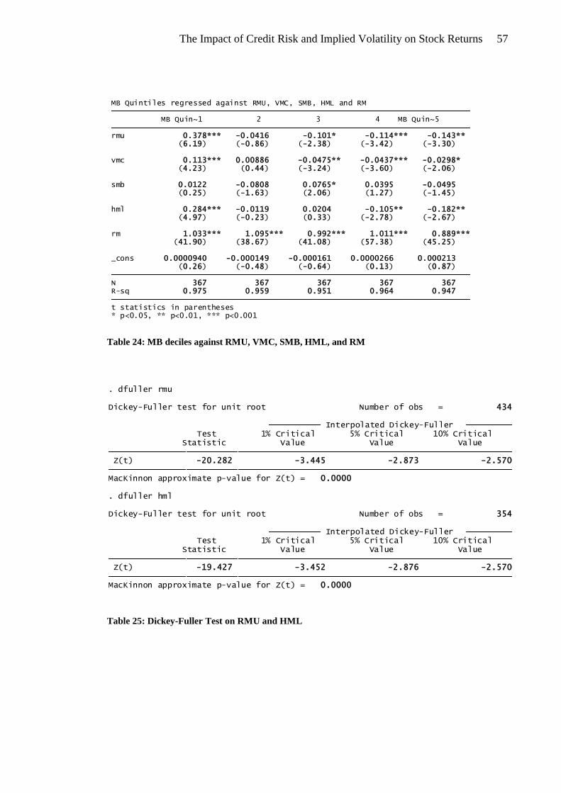
The Impact of Credit Risk and Implied Volatility on Stock Returns 57
Table 24: MB deciles against RMU, VMC, SMB, HML, and RM
Table 25: Dickey-Fuller Test on RMU and HML
* p<0.05, ** p<0.01, *** p<0.001t statistics in parentheses R-sq 0.975 0.959 0.951 0.964 0.947 N 367 367 367 367 367 (0.26) (-0.48) (-0.64) (0.13) (0.87) _cons 0.0000940 -0.000149 -0.000161 0.0000266 0.000213
(41.90) (38.67) (41.08) (57.38) (45.25) rm 1.033*** 1.095*** 0.992*** 1.011*** 0.889***
(4.97) (-0.23) (0.33) (-2.78) (-2.67) hml 0.284*** -0.0119 0.0204 -0.105** -0.182**
(0.25) (-1.63) (2.06) (1.27) (-1.45) smb 0.0122 -0.0808 0.0765* 0.0395 -0.0495
(4.23) (0.44) (-3.24) (-3.60) (-2.06) vmc 0.113*** 0.00886 -0.0475** -0.0437*** -0.0298*
(6.19) (-0.86) (-2.38) (-3.42) (-3.30) rmu 0.378*** -0.0416 -0.101* -0.114*** -0.143** MB Quin~1 2 3 4 MB Quin~5 MB Quintiles regressed against RMU, VMC, SMB, HML and RM
MacKinnon approximate p-value for Z(t) = 0.0000 Z(t) -19.427 -3.452 -2.876 -2.570 Statistic Value Value Value Test 1% Critical 5% Critical 10% Critical Interpolated Dickey-Fuller
Dickey-Fuller test for unit root Number of obs = 354
. dfuller hml
MacKinnon approximate p-value for Z(t) = 0.0000 Z(t) -20.282 -3.445 -2.873 -2.570 Statistic Value Value Value Test 1% Critical 5% Critical 10% Critical Interpolated Dickey-Fuller
Dickey-Fuller test for unit root Number of obs = 434
. dfuller rmu