ISSN 1178-2293 (Online)

University of Otago Economics Discussion Papers

No. 1706

APRIL 2017

The impact of climate change on crop production in Ghana:

A Structural Ricardian analysis

Prince M. Etwire§,†

David Fielding§,¶

Viktoria Kahui§

§ Department of Economics, PO Box 56, Dunedin 9054, New Zealand.

† CSIR-Savanna Agricultural Research Institute, PO Box 52, Tamale, Ghana ¶ Corresponding author: e-mail: david.fielding@otago.ac.nz; telephone +64 3 479 8653.

1

The impact of climate change on crop production in Ghana: A

Structural Ricardian analysis

Prince M. Etwire§,†

David Fielding§,¶

Viktoria Kahui§

Abstract

We apply a Structural Ricardian Model (SRM) to farm-level data from Ghana in order to

estimate the impact of climate change on crop production. The SRM explicitly incorporates

changes in farmers’ crop selection in response to variation in climate, a feature lacking in

many existing models of climate change response in Africa. Two other novel features of our

model are an estimate of the response of agricultural profits to differences in land tenure, and

a comprehensive investigation of the appropriate functional form with which to model

farmers’ responses. This final feature turns out to be important, since estimates of the effect

of climate change turn out to be sensitive to the choice of functional form.

JEL classification: O13; O55; Q12; Q54

Keywords: Structural Ricardian Model; climate change; Ghana

§ Department of Economics, PO Box 56, Dunedin 9054, New Zealand.

† CSIR-Savanna Agricultural Research Institute, PO Box 52, Tamale, Ghana ¶ Corresponding author: e-mail: david.fielding@otago.ac.nz; telephone +64 3 479 8653.

2

1. Introduction

Many developing countries are especially sensitive to climate change because they are

located in the tropics, with temperatures that already compromise agricultural production (Da

Cunha et al., 2015; Kurukulasuriya et al., 2006; Mendelsohn et al., 2006), and because they

have limited access to the human and physical capital that might mitigate its effects (Di

Falco, 2014). These challenges are often compounded by a lack of access to new technology

and to developed markets (Di Falco, 2014; Kurukulasuriya et al., 2006). Ghana is one

example of a country facing these challenges. Less than 1% of its land is under irrigation and

the vast majority of its farmers rely entirely on rainfall (MoFA, 2010; 2014; World Bank,

2010).

In this paper we present estimates of the effect of climate change on Ghana based on

the application of a Structural Ricardian Model (SRM) to a large microeconomic dataset. The

first stage in the model is designed to estimate farmers’ crop choices – a feature that is absent

from many other estimates of climate change effects in developing countries – while the

second stage is designed to estimate farm revenue conditional on these choices. The model is

then used to simulate the impact of climate change under various climate scenarios. Our

model incorporates two other innovative features absent from many applications of the SRM.

Firstly, we explicitly allow crop choice to depend on the form of land tenure, which is known

to affect agricultural production through its impact on investment decisions and access to

credit (Fenske, 2011). Secondly, we apply the model in a way that allows for a variety of

alternative functional forms. Our results turn out to be highly sensitive to the choice of

functional form, and we find that inappropriate functional form restrictions can lead to

misleading results. In this respect our findings are in line with the Italian study of De Salvo et

al. (2013).1

1 Other authors, for example Fezzi and Bateman (2013), have found results that are not sensitive to

3

2. An overview of the SRM

In a traditional Ricardian model of farm productivity, farmers are assumed to allocate their

land to different crops so as to maximize profit, and therefore land values reflect the present

discounted value of future farm revenue (Mendelsohn et al., 1994; 1996). This model has

been criticised for failing to pay sufficient attention to the factors that drive crop selection

(Elbehri and Burfisher, 2015; Kurukulasuriya and Mendelsohn, 2008; Seo and Mendelsohn,

2008), and the SRM addresses this criticism by incorporating an explicit model of the

farmer’s choice of crops. In our version of the model, assume that the desirability of crop j on

plot i is given by:

𝑦𝑖𝑖∗ = 𝛽𝑖𝑥𝑖 + 𝑣𝑖𝑖 (1)

Here, 𝑥𝑖 stands for a vector of farm characteristics and 𝛽𝑖 stands for a vector of parameters to

be estimated. If the error term 𝑣𝑖 is drawn from a Gumbel Distribution and if the farmer of

plot i chooses the most desirable crop, then the probability that crop j will be chosen out of J

alternatives (𝑃𝑖𝑖) is given by the following equation (McFadden, 1973):2

𝑃𝑖𝑖 = exp�𝛽𝑗𝑥𝑖�

∑ exp(𝛽𝑘𝑥𝑖)𝑘=𝐽𝑘=0

(2)

Suppose further that the annual net revenue per hectare from crop j (𝜑𝑖𝑖) is given by the

following function:

functional form restrictions, but our results add weight to the argument that such restrictions should not be

assumed a priori. 2 This specification of the first-stage regression equation assumes the Independence of Irrelevant

Alternatives (IIA). Bourguignon et al. (2007) find that violation of the IIA assumption does not impair the

consistency of the estimates of the second-stage regression equation, i.e. equation (4) below. Nevertheless,

we tested for violation of the IIA assumption using the method of Small and Hsiao (1985). Using this test,

we cannot reject the IIA assumption at conventional confidence levels.

4

𝜑𝑖𝑗(𝜃)−1𝜃

= 𝛼𝑖𝑧𝑖 + 𝑤𝑖𝑖 (3)

Here, 𝑧𝑖 stands for a vector of farm characteristics (excluding at least one of the 𝑥𝑖 variables),

𝛼𝑖 stands for another vector of parameters to be estimated, and 𝑤𝑖𝑖 stands for a normally

distributed error term. The left hand side of equation (3) is a Box-Cox transformation

incorporating the parameter 𝜃 (Box and Cox, 1964). Direct estimation of this equation is

likely to suffer from selection bias but, having fitted equation (2) to the data using a

multinomial logit model, the bias can be corrected by fitting the following equation (Dubin

and McFadden, 1984; Bourguignon et al., 2007; Seo and Mendelsohn, 2008):

𝜑𝑖𝑗(𝜃)−1

𝜃= 𝛼𝑖𝑧𝑖 + 𝜎 √6

п∑ 𝑟𝑘𝑖 ∙ �

𝑃𝑖𝑘𝑙𝑙(𝑃𝑖𝑘)1−𝑃𝑖𝑘

+ 𝑙𝑙(𝑃𝑖𝑖)�𝑘≠𝑖 + 𝑤𝑖𝑖 (4)

Here, 𝑟𝑘𝑖 = 𝑐𝑐𝑟𝑟�𝑤𝑖𝑖, 𝑣𝑖𝑘� and 𝜎 is a variance parameter; 𝜎 ∙ 𝑟𝑘𝑖 can be estimated directly.

See De Salvo et al. (2013) for a previous SRM application of the Box-Cox

transformation. This transformation allows the equation for net revenue to take a range of

alternative functional forms, encompassing equations in levels (e.g. Coster and Adeoti, 2015;

Fleischer et al., 2008; Kurukulasuriya and Ajwad, 2007; Mendelsohn et al., 1996; Seo and

Mendelsohn, 2008) as well as inverse and semi-logarithmic functions (e.g. Chatzopoulos and

Lippert, 2015; Fezzi and Bateman, 2013). Another attractive feature of Box-Cox

transformation is its ability to compensate for heteroscedasticity (Blaylock et al., 1980). In

the special case of 𝜃 = 1 we have a model in levels, in the case of 𝜃 = 0 we have a

logarithmic model, and in the case of 𝜃 = –1 we have an inverse transformation (Box and

Cox, 1964).

In our application of the model, the 𝑥𝑖 variables in equations (1-2) comprise the

following features:

5

tempi: the mean temperature observed on plot i, and (tempi)2.

precipi: mean precipitation observed on plot i, and (precipi)2.

tenurei: the form of land tenure applicable to plot i.

soili: a measure of soil quality on plot i.

agei: the age in years of the head of the household farming plot i.

malei = 1 if the head of the household farming plot i is male; otherwise malei = 0.

non-farm-incomei: the gross non-farm income of the household farming plot i.

The 𝑧𝑖 variables in equations (3-4) comprise all of these features except non-farm-incomei.

Non-farm income allows the household to bear periods with no income from crops, and so to

plant crops which take a long time to grow; in Ghana this is particularly relevant to plantain,

which is a perennial crop. It is also likely that non-farm income will be positively associated

with the cultivation of maize, which is especially reliant on costly inputs such as inorganic

fertilizers, pesticides and weedicides (Coster and Adeoti, 2015; Kanton et al., 2016).

However, non-farm income should not affect the productivity of the land once the crop has

been planted.3

3. Data

The data for 𝜑𝑖𝑖, tenurei, agei, malei, and non-farm-incomei are taken from the sixth round of

the Ghana Living Standards Survey (GLSS), published by the Ghana Statistical Service. This

survey was implemented between 18 October 2012 and 17 October 2013 (Ghana Statistical

Service, 2014). The results below are based on observations for the 6,321 farming households

in the sample. For the dependent variables 𝜑𝑖𝑖, net revenue is measured as the total US Dollar

3 It turns out that the correlation between temp and (temp)2 makes estimates of non-linear temperature

effects in second-stage model of revenue very imprecise, so in results reported below (temp)2 is omitted at

the second stage. However, our a priori identification restriction is on non-farm-income.

6

value of crop j less production costs, as reported by the head of the household farming plot i.4

Our analysis is confined to the most important income-generating crops in Ghana: maize (Zea

mays), rice (Oryza spp), cassava (Manihot esculenta), plantain (Musa spp), groundnuts

(Arachis hypogaea), and millet (Pennisetum glaucum). Tenurei is measured as a binary

variable indicating whether the land is communal (tenurei = 0) or private (tenurei = 1). We

define private land as land that the household has procured individually, has long-term rights

to, and can use for any purpose. Communal land belongs to the extended family or to the

community, and the household has no property rights over this land, which accounts for about

80% of all farmland in Ghana (Pande and Udry, 2005). Farmers with private land are usually

able to recoup the investments they make, but investment in communal land carries no such

guarantee. We anticipate that farmers will be more likely to invest in their land if it is owned

privately (Kurukulasuriya and Ajwad, 2007), increasing net revenue. We also anticipate that

net revenue will be higher if the household head is male. Households with female heads may

have less access to resources, or face discrimination in the market place, or have fewer men

to work in the fields when the women have childcare responsibilities (Coster and Adeoti,

2015; Kurukulasuriya and Ajwad, 2007). The effect of age on revenue could be positive, if it

associated with greater experience (Coster and Adeoti, 2015; Fleischer et al., 2008), or

negative, if households with older heads are less physically capable.

The climate variables (tempi, precipi) are constructed from historical weather station

data for the period 1973-2011 (National Oceanic and Atmospheric Administration, 2015).

We match the GLSS data to the climate data at a spatial resolution of one degree. Tempi is

defined as the mean recorded temperature over the period (in degrees centigrade) and precipi

4 A plot is defined as all land allocated to a particular crop by a single household.

7

is defined as mean recorded precipitation (in millimetres).5,6 The variable soili is constructed

from data provided by the Soil Research Institute of Ghana’s Council for Scientific and

Industrial Research (CSIR-SRI). Soili = 1 indicates relatively fertile soil (soil types I-IV as

defined by the CSIR-SRI) while soili = 0 indicates relatively infertile soil (types V-VI).7

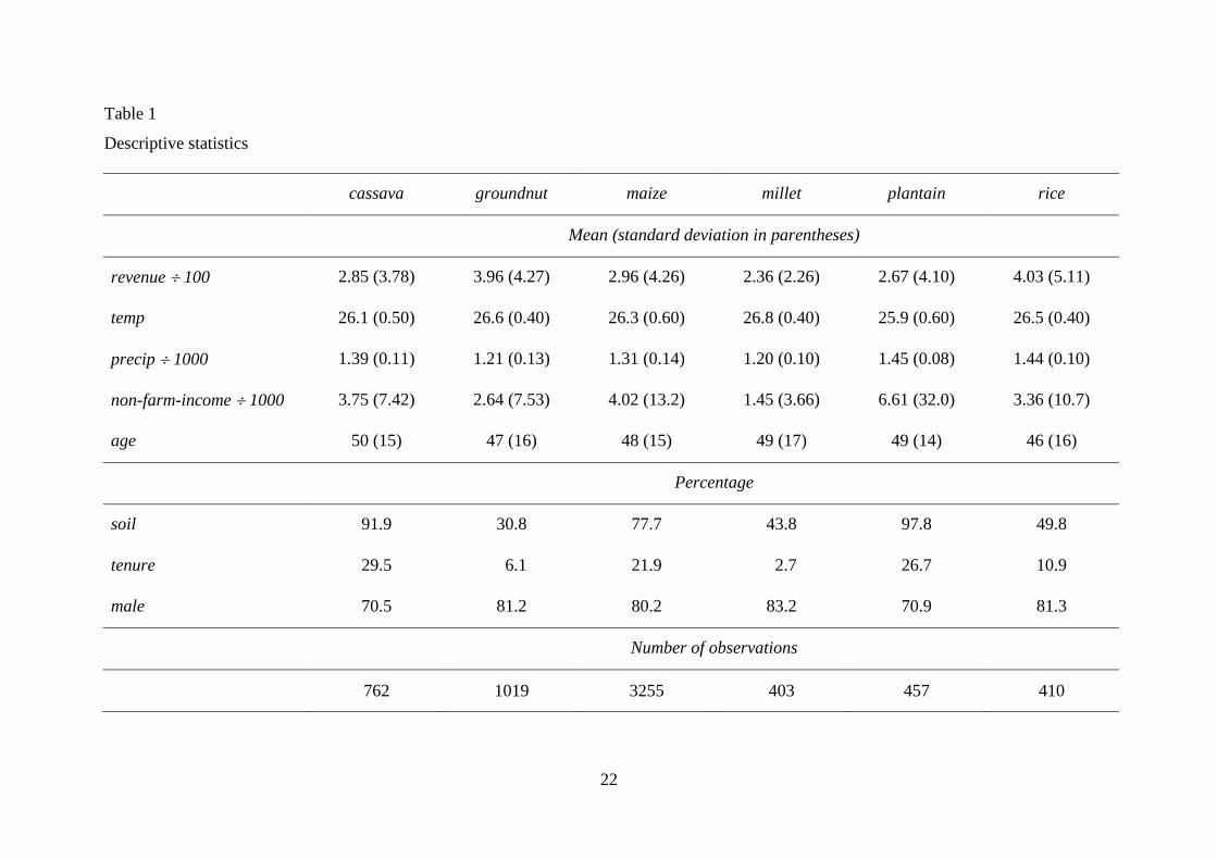
Table 1 reports descriptive statistics for the variables in our model disaggregated by

crop. The table shows some strong associations between crop type and farm characteristics,

although it is important to note that these are unconditional associations. Rice, plantain and

cassava tend to be cultivated in relatively high-precipitation areas while millet and

groundnuts are cultivated in relatively low-precipitation areas; maize represents an

intermediate case. Plantain, cassava and maize are also associated with relatively fertile soil,

while groundnuts and millet are associated with relatively infertile soil; rice represents an

intermediate case. There is no substantial variation in the mean temperature associated with

the different crops. Average net revenues from rice and groundnut cultivation are much

higher than for other crops. Plantain cultivation is associated with relatively high non-farm

income and millet cultivation with relatively low non-farm income. For all crops, however,

there is substantial variation across households in both the net revenue from the crop and the

5 Alternatively, we might include seasonal climate variables, for example mean temperature and

precipitation for each month or for each quarter of the year. However, the seasonal measures in our dataset

are highly collinear and have no significant explanatory power in our model. 6 A model incorporating spatially interpolated climate variables may suffer from an errors-in-variables

problem (Chatzopoulos and Lippert, 2015). In order to explore this potential problem, we fitted a model in

which latitude, longitude, visibility, maximum sustained wind speed and sea level pressure were used as

instruments for temp and precip. Using the Wooldridge Score Test (Wooldridge, 1995), it was not possible

to reject the null hypothesis that temp and precip are exogenous at conventional confidence levels. 7 Soil type I is non-gravelly and medium to moderately heavy textured. Soil type II is medium to

moderately heavy textured but gravelly. Soil type III, which is mostly alluvial, may contain gravelly and

moderately shallow soil or heavy plastic clay. Soil type IV is shallow and imperfectly drained. Soil type V

comprises poorly drained soils or terraced-derived soils containing pebbles. Soil type VI is very saline.

Adding indicator variables for individual soil types does not produce statistically significant coefficients.

8

non-farm income of the households cultivating it. There is a relatively high proportion of

households with female heads farming the perennial crops, cassava and plantain, and these

crops are also associated with a relatively high incidence of private land tenure. There is little

variation in the average age of the household head across different types of crop.

4. Modelling the impact of climate change on crop production

4.1. The selection equation

Individual parameter estimates from the multinomial crop selection model in equation (2) are

presented in Appendix 1. A Wald χ2 test shows that the explanatory variables are jointly

significant at the 1% level, while the count R2 statistic indicates that the regressors explain

over 50% of the variation in crop selection. Table 2 presents the corresponding marginal

effects for all variables except temp and precip, evaluated at the mean shares of each crop,

along with heteroscedasticity-robust standard errors. Table 2 shows marginal effects that are

somewhat different from the unconditional associations in Table 1, which reflects significant

correlations across the different explanatory variables and suggests that great care should be

taken when interpreting the unconditional associations.

Table 2 shows that higher soil quality is associated with a significantly greater

probability of cultivating maize and cassava (and plantain, although this effect is relatively

small), while the other crops – groundnuts, rice and millet – are associated with low-quality

soils. It is already known that maize requires especially fertile soil (Coster and Adeoti, 2015;

Kanton et al., 2016), and that groundnuts are particularly suitable for low-quality land

because of their ability to fix atmospheric nitrogen (Kombiok et al., 2012). Perennial crops

such as cassava and plantain may be allocated to more fertile soils in order to minimize soil

improvement costs. The table also shows that private land tenure is associated with a

significant rise in the probability of maize cultivation and a significant fall in the probability

of groundnut, millet and plantain cultivation. One possible explanation for these effects is

9

that efficient maize cultivation is associated with long-term investments that are larger, on

average, than for other crops, and that private land tenure incentivizes such investments.

However, differences in capital investments across crops are not well documented, so this is a

topic for future research.

Age and sex of the household head also have significant effects on crop selection.

Older farmers are more likely to select cassava but less likely to select groundnuts and rice.

One possible explanation, which requires further research, is that groundnuts and rice are

more likely to be sold at market, while cassava is more likely to be consumed by the

household, and that food makes up a greater share of the total consumption of households

with older heads. Households with female heads are more likely to cultivate the perennial

crops (cassava and plantain) and less likely to cultivate millet and maize; these effects are

statistically significant. Cassava and plantain require some post-harvest processing in order to

preserve them, and these tasks are often undertaken by women (African Development Fund,

2008). Moreover, cassava and plantain are harvestable throughout the year (Dziedzoave et

al., 2006), so a household specializing in these crops will not have to compete with other

farmers for tractors and casual labour at the beginning of the season. This makes them

particularly suitable for households with less bargaining power in the local community.

As anticipated, higher non-farm income is associated with a greater probability of

maize and plantain cultivation. It is also associated with a smaller probability of millet

cultivation; these effects are statistically significant.

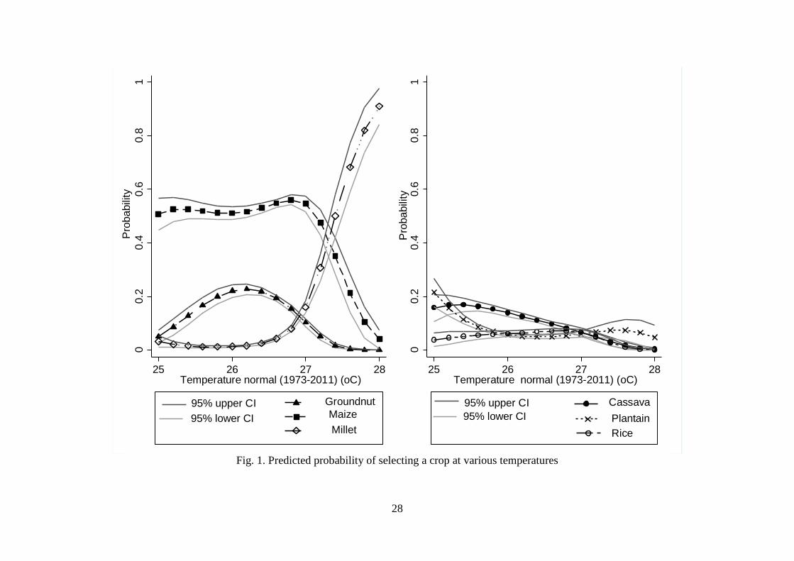
The inclusion of quadratic terms in temp and precip allows the effect of these

variables to be non-monotonic, so Figures 1-2 show the predicted probability of the selection

of different crops at different temperature and precipitation levels, along with the

corresponding 95% confidence interval. These effects are estimated at the mean values of the

other regressors. Figure 1 shows that at moderate temperatures (below 26.5 degrees

10

centigrade) around 60% of the land is under maize cultivation and almost no land is under

millet cultivation. Above 26.5 degrees there is substantial switching from maize to millet, and

at 28 degrees almost all of the land is under millet cultivation. See Aidoo et al. (2016) for a

discussion of the characteristics of millet which make is especially tolerant of high

temperatures. Rises in temperature are associated with a gradual decline in the proportion of

land devoted to cassava and (to a lesser extent) plantain: at 25 degrees these crops together

account for about 40% of the land under cultivation, this figure dropping to almost zero at 28

degrees. Groundnuts account for about 20% of land under cultivation at mid-range

temperatures (25.5-26.5 degrees), but a very small proportion outside this range. The

cultivation of rice is relatively invariant to temperature.

Figure 2 shows that there are several non-monotonic precipitation effects. The

cultivation of the annual crops (maize, groundnuts, rice and millet) is most frequent at

intermediate precipitation levels. Maize cultivation reaches a peak at 1200mm of rainfall,

millet at 1400mm, groundnuts at 1500mm, and rice at 1700mm. In extremely dry conditions

(below 1100mm), only 40% of the land is allocated to maize and almost no land is allocated

to the other annual crops. In extremely wet conditions (above 1800mm), almost no land is

allocated to any of the annual crops. At extreme levels of precipitation the dominant crop is

cassava. Cassava has an extensive root system that protects it from drought and is robust

enough to withstand high rainfall (Dziedzoave et al., 2006).

4.2. The revenue equation

Table 3 presents estimates of the parameters in equation (4). Estimates of the θ parameter for

each crop range from 0.07 to 0.18: these numbers are significantly greater than zero but

significantly less than one (p < 0.05 in all cases), so we can reject the linear, inverse, and log-

linear specifications of the SRM. For each crop, the first column in the table reports the

parameter estimates in the unrestricted model (with a fitted value of θ), while subsequent

11

columns reports parameter estimates from a semi-log-linear model (imposing θ = 0) and from

a linear model (imposing θ = 1). Here we concentrate mainly on the results in the first

column, while the other columns show how the results differ if a specific functional form is

assumed. The Box-Cox transformation is non-linear, so the coefficients cannot be compared

directly across the columns, and further results comparing individual marginal effects in the

different models are available on request. The rest of this section discusses the sign and

statistical significance of different effects, leaving the discussion of the size of the effects of

climate change in the different models to the next section.

Before discussing estimates of the α coefficients in Table 3, we note that several of

the selection effects (𝑟𝑘𝑖) are significant at the 5% level. Restricting attention to the first

column for each crop (i.e. our preferred model), all but one of these significant effects is

negative: that is, a plot which is predicted to be used for crop k but is instead used for crop j

can be expected to generate less revenue from this crop than otherwise. One interpretation of

these effects is that the average household is making reasonably efficient crop selection

decisions. These decisions are characterized in Table 2, and households which deviate from

the average are less efficient. The one exception is that maize plots which are predicted to be

used for plantain generate higher revenue than otherwise. However, this represents a single

anomalous coefficient out of 25.

In interpreting the effect of temperature in equation (4), it is important to remember

that the different crops are typically grown in different climatic ranges. Of the three crops

showing a significant negative effect of temperature on revenue, one (millet) is the crop

which predominates at very high temperatures, while the other two (plantain and rice) have a

probability of selection that is relatively invariant to temperature. The crops which show the

largest reductions in the probability of selection at very high temperatures in Figure 1

12

(cassava, groundnuts and maize) show positive temperature effects in Table 3,8 although in

the Box-Cox model these effects are statistically insignificant. One interpretation of the Table

3 results is that when temperatures are high enough to threaten the yields of cassava,

groundnuts or maize, farmers immediately substitute into millet, which is the most heat-

tolerant crop. One might ask whether farmers substitute too readily into millet. The absence

of positive millet selection effects (𝑟𝑚𝑖𝑙𝑙𝑚𝑚𝑖) in Table 3 suggests that farmers are generally

making the right decisions about when to grow millet; however, the absence of negative

temperature effects for cassava, groundnuts and maize suggests further research into the

relative returns to millet production at the critical temperature margin, around 27 degrees.9

The two crops for which there is an effect of land tenure on revenue that is significant

at the 5% level are cassava and maize. This is consistent with the Table 2 results: private land

tenure is also associated with a greater probability of maize and cassava cultivation, although

the second effect is not statistically significant. For all crops except plantain, the sex of the

household head has a significant effect on revenue. Ceteris paribus, households with female

heads are earning revenues that are about half as large as those of other households. Similar

results appear in Coster and Adeoti (2015) and in Kurukulasuriya and Ajwad (2007), who

suggest that this effect can be explained by differential access to productive resources and

discrimination in the market place. The one crop for which there is a significant effect of the

age of the household head on revenue is maize. The effect is negative, as in Ajetomobi et al.

(2010) but in contrast to Coster and Adeoti (2015) and Fleischer et al. (2008), who find a

positive effect, and Issahaku and Maharjan (2014) and Kurukulasuriya and Ajwad (2007),

8 The results for cassava and rice are consistent with those in Issahaku and Maharjan (2014). 9 As noted above, parameter estimates in a model including both temp and (temp)2 are very imprecisely

estimated, and it is not possible to determine whether the marginal effect of temperature on yield varies

across the range. If there were evidence of a positive effect of temperature on maize revenues at the upper

extent of the relevant range then one could argue more strongly that farmers are switching too soon.

13

who find no significant effect. The relative importance of experience and physical capability

may well vary across households and crops, so it is unlikely that our results for age can be

generalized.

The one anomalous result in Table 3 is that there is a negative and significant

association between soil quality and net revenue from cassava and maize. One possible

reason for this effect is that cassava and maize farmers over-invest in the improvement of

fertile soils, but establishing the true cause of this effect is a subject for future research.

5. Simulating impact of climate change on agricultural revenue

We rely on the latest temperature and precipitation projections of the Intergovernmental

Panel on Climate Change (IPCC) (Christensen et al., 2013) to simulate the impact of climate

change on agricultural revenue in Ghana. These projections are based on Phase Five of the

Coupled Model Inter-comparison Project (CMIP5), which collates results from 39 different

global models. We use the projections for West Africa up to the year 2035. Three different

IPCC scenarios are considered. Under the first and ‘most optimistic’ scenario, temperature is

projected to increase by 0.7 degrees and precipitation by 8%. These increases represent the

minimum projected increase in temperature and maximum projected increase in precipitation.

The second scenario corresponds to the median increase in temperature (0.9 degrees) and in

precipitation (1%). The third and ‘least optimistic’ scenario corresponds to the maximum

projected increase in temperature (1.5 degrees) and maximum decline in precipitation (4%).

Table 4 presents the simulated change in the probability of selecting each crop under

the three different scenarios, while Table 5 presents the simulated change in in revenue.10 In

10 An important caveat here is that given the way in which the projections have been constructed, it is not

possible to compute standard errors around these simulations. The simulations also assume no change in

any of the other characteristics affecting crop selection and revenue.

14

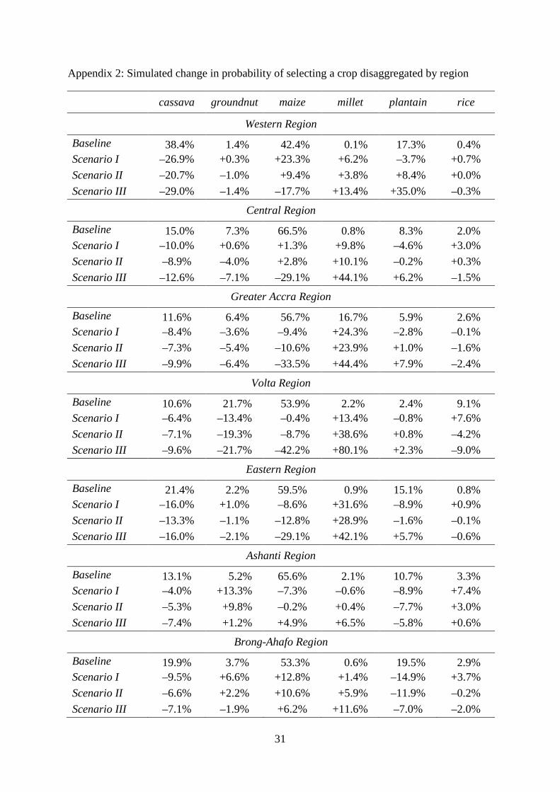
Appendices 2-3 we present a regional disaggregation of these results.11 The main feature of

Table 4 is that rising temperatures are associated with the increasing selection of millet and

decreasing selection of other crops. Millet currently accounts for just over 6% of all plots:

under the third and most extreme scenario this percentage is projected to increase tenfold.

Maize currently accounts for just over 50% of all plots: under the third scenario this

percentage is projected to fall by more than half. There are also substantial reductions in the

cultivation of cassava, plantain, groundnuts and rice: in the third scenario these last two crops

disappear almost entirely.

Table 5 presents the results for revenue, including simulations based on all three of

the models in Table 3 (θ estimated, θ = 0, and θ = 1). For the first two of these models, which

are nonlinear, it is necessary to compute marginal effects for the discrete changes in

temperature and precipitation. For the Box-Cox model (θ estimated) we employ the two-stage

smearing method of Abrevaya (2002), which is an extension of Duan (1983). For the log-

linear model (θ = 0) we use the extension of Duan proposed by Baum (2009). The signs of

the effects are mostly consistent across the three models, but the sizes of the effects vary

substantially, especially when comparing the linear model with the other two. Moreover, for

millet, which is projected to become the most important crop in Ghana, the signs of the

effects do vary across models. This means that finding the correct functional form for the

revenue equation is essential for producing accurate climate change predictions. Given that

the restrictions θ = 0 and θ = 1 can be rejected on our data we suggest that the simulations

based on the Box-Cox model are the most reliable.12

11 The appendices show that there is substantial inter-regional variation in the magnitude of the effects, as

has been found in other countries – see for example Wang et al. (2009). 12 In some cases the linear model predicts negative revenue for a particular crop. We have left these

predictions in Table 5, but this is another reason for being sceptical about any predictions based on this

model.

15

The most striking feature of the Box-Cox results in Table 5 is that there are only two

cases in which there is any substantial change in revenue: under the first scenario there are

moderate increases in cassava and rice revenue resulting from the increased precipitation.

However, these two crops account for only a small proportion of total land use. For other

crops (and for cassava and rice under the other scenarios) the predicted changes are very

small. Another way of putting this result is that for each crop, the estimated effects of

temperature and precipitation on revenue using the existing survey data are sometimes

statistically significant but nevertheless generally quite small: the variation within the

climatic range typical of each crop does not have large effects. However, as illustrated in

Figures 1-2, there is substantial variation in the climatic conditions associated with each crop.

Therefore, the effects of climate change on total agricultural revenue will be dominated by

crop selection effects. In the baseline case corresponding to current climatic conditions, the

estimated net revenue from millet for a household with average characteristics is about $240

per hectare. The next lowest figure is for plantain ($270), followed by cassava ($290), maize

($300), and then groundnuts and rice ($400). The Box-Cox results in Table 5 suggest that

these figures are unlikely to change by very much, but the results in Table 4 suggest that

groundnut and rice cultivation will plummet and millet will supplant maize as the

predominant crop.

6. Summary and conclusion

We apply a Structural Ricardian Model to farm-level data from Ghana in order to estimate

the impact of climate change on crop selection and revenue from production. We find that

both crop selection and revenue are associated with a range of characteristics of the

household and its land. Non-farm income, soil quality and the form of land tenure have

substantial effects, and we find evidence suggesting that households with female heads are

considerably disadvantaged. Conditional on these effects, local temperature and precipitation

16

have large and asymmetric effects on crop selection decisions; they also have some effect on

revenue from individual crops. One novel feature of our approach is the use of a Box-Cox

transformation to model effects on revenue. We find that the simple functional forms that

have been used in previous studies – for example a linear or log-linear function – can be

rejected on our data. Alternative function forms lead to widely varying estimates of the size

of the effects of temperature and precipitation on revenue, so this is not a trivial issue.

Our simulations of the effect of climate change are derived by combining the results

of our statistical model with climate forecasts from the Intergovernmental Panel on Climate

Change. These simulations suggest that climate change will have large effects on crop

selection decisions: in particular, there will be substantial substitution of millet for maize

(which is currently the most important food crop), and the cultivation of other crops such as

groundnuts and rice will fall dramatically. Because of this adaptation, with farmers relying

increasingly heavily on heat-tolerant millet, there are unlikely to be large effects on the

revenue per hectare from individual crops. Although the overall volume of crop production

might not change very much, overall revenue is likely to fall substantially, because millet is

the least profitable of all existing crops, while groundnuts and rice are the most profitable.

Our results also suggest some ways in which the decline in revenue might be

mitigated. Over the range of moderate temperatures at which maize cultivation is currently

observed, higher temperatures do not reduce revenue, and it is possible that farmers switch

too readily from maize to millet when temperatures rise, suggesting the need for incentives to

encourage maize production. One policy might be to extend private land tenure, which is

strongly associated with both a propensity to cultivate maize and with revenues from maize

cultivation. However, even if such measures do mitigate the decline in revenue, Ghana may

have to look to alternative, non-agricultural sources of income in the future.

17

References

Abrevaya, J. (2002) ‘Computing marginal effects in the Box–Cox model.’ Econometric

Reviews, 21: 383-393.

African Development Fund. (2008) Ghana Country Gender Profile. Abidjan.

Aidoo, M.K., E. Bdolach, A. Fait, N. Lazarovitch and S. Rachmilevitch (2016) ‘Tolerance to

high soil temperature in foxtail millet (Setaria italica L.) is related to shoot and root

growth and metabolism.’ Plant Physiology and Biochemistry, 106: 73-81.

Ajetomobi, J.O., A. Abiodun and R. Hassan (2010) ‘Economic impact of climate change on

irrigated rice agriculture in Nigeria.’ Paper presented at the third African Association of

Agricultural Economists Conference and the 48th Agricultural Economists Association of

South Africa Conference, Cape Town, South Africa, September 19-23.

Baum, C.F. (2009) ‘LEVPREDICT: Stata module to compute log-linear level predictions

reducing retransformation bias.’ Statistical Software Component S457001, Boston

College Department of Economics.

Blaylock, J., L. Salathe and R. Green (1980) ‘A note on the Box-Cox Transformation under

heteroscedasticity.’ Western Journal of Agricultural Economics, 129-135.

Bourguignon, F., M. Fournier and M. Gurgand (2007) ‘Selection bias corrections based on

the multinomial logit model: Monte Carlo comparisons.’ Journal of Economic Surveys,

21(1): 174-205.

Box, G.E.P. and D.R. Cox (1964) ‘An analysis of transformations.’ Journal of the Royal

Statistical Society Series B, 26: 211-243.

Chatzopoulos, T. and C. Lippert (2015) ‘Adaptation and climate change impacts: A structural

Ricardian analysis of farm types in Germany.’ Journal of Agricultural Economics, 66(2):

537-554.

Christensen, J.H., K.K. Kumar, E. Aldrian, S.I. An, I.F.A. Cavalcanti, M. De Castro, W.

18

Dong, P. Goswami, A. Hall, J.K. Kanyanga, A. Kitoh, J. Kossin, N.C. Lau, J. Renwick,

D.B. Stephenson, S.P. Xie and T. Zhou (2013) ‘Climate phenomena and their relevance

for future regional climate change supplementary material.’ In T.F. Stocker et al. (eds.)

Climate Change: The Physical Science Basis. Contribution of Working Group I to the

Fifth Assessment Report of the Intergovernmental Panel on Climate Change, New York,

NY, 1217-1308.

Coster, A.S. and A.I. Adeoti (2015) ‘Economic effects of climate change on maize

production and farmers’ adaptation strategies in Nigeria: A Ricardian approach.’ Journal

of Agricultural Science, 7(5): 67-84.

Da Cunha, D.A., A.B. Coelho and J.G. Féres (2015) ‘Irrigation as an adaptive strategy to

climate change: an economic perspective on Brazilian agriculture.’ Environment and

Development Economics, 20(1): 57-79.

De Salvo, M., Raffaelli and R. Moser (2013) ‘The impact of climate change on permanent

crops in an Alpine region: A Ricardian analysis.’ Agricultural Systems, 118: 23-32.

Di Falco, S. (2014) ‘Adaptation to climate change in Sub-Saharan agriculture: assessing the

evidence and rethinking the drivers.’ European Review of Agricultural Economics, 41(3):

405-430.

Duan, N. (1983) ‘Smearing estimate: A nonparametric retransformation method.’ Journal of

the American Statistical Association, 78: 605-610.

Dubin, J. A. and D. L. McFadden (1984) ‘An econometric analysis of residential electric

appliance holdings and consumption.’ Econometrica, 52: 345–362.

Dziedzoave, N.T., A.B. Abass, W.K.A. Amoa-Awua and M. Sablah (2006) Quality

Management Manual for the Production of High Quality Cassava Flour. Ibadan:

International Institute of Tropical Agriculture.

Elbehri, A. and M. Burfisher (2015) ‘Economic modelling of climate impacts and adaptation

19

in agriculture: A survey of methods, results and gaps.’ In A. Elbehri (ed.). Climate

Change and Food Systems: Global Assessments and Implications for Food Security and

Trade. Rome: Food Agriculture Organization, 60-105.

Fenske, J. (2011) ‘Land tenure and investment incentives: Evidence from West Africa.’

Journal of Development Economics, 95(2): 137-156.

Fezzi, C. and I. Bateman (2015). ‘The impact of climate change on agriculture: Nonlinear

effects and aggregation bias in Ricardian models of farmland values.’ Journal of the

Association of Environmental and Resource Economists, 2(1): 57-92.

Fleischer, A., I. Lichtman and R. Mendelsohn (2008) ‘Climate change, irrigation, and Israeli

agriculture: Will warming be harmful?’ Ecological Economics, 65(3): 508-515.

Ghana Statistical Service (2014) Ghana Living Standards Survey Round 6 Main Report.

Accra.

Issahaku, Z.A. and K.L. Maharjan (2014) ‘Climate change impact on revenue of major food

crops in Ghana: Structural Ricardian cross-sectional analysis.’ In K.L. Maharjan (ed.)

Communities and Livelihood Strategies in Developing Countries. Tokyo: Springer, 13-32.

Kanton, R.A.L., P.V.V. Prasad, A.M. Mohammed, J.K. Bidzakin, E.Y. Ansoba, P.A.

Asungre, S. Lamini, G. Mahama, F. Kusi and I. Sugri (2016) ‘Organic and inorganic

fertilizer effects on the growth and yield of maize in a dry agro-ecology in northern

Ghana.’ Journal of Crop Improvement, 30(1): 1-16.

Kombiok, J.M., S.S.J. Buah, I.K. Dzomeku and H. Abdulai (2012) ‘Sources of pod yield

losses in groundnut in the northern Savanna Zone of Ghana.’ West African Journal of

Applied Ecology, 20(2): 53-63.

Kurukulasuriya, P. and M.I. Ajwad (2007) ‘Application of the Ricardian technique to

estimate the impact of climate change on smallholder farming in Sri Lanka.’ Climatic

Change, 81(1): 39-59.

20

Kurukulasuriya, P. and R. Mendelsohn (2008) ‘Crop switching as a strategy for adapting to

climate change.’ African Journal of Agricultural and Resource Economics, 2(1): 105-126.

Kurukulasuriya, P., R. Mendelsohn, R. Hassan, J. Benhin, T. Deressa, M. Diop, H.M. Eid,

K.Y. Fosu, G. Gbetibouo, S. Jain, A. Mahamadou, R. Mano, J. Kabubo-Mariara, S. El-

Marsafawy, E. Molua, S. Ouda, M. Ouedraogo, I. Se´ne, D. Maddison, S.N. Seo and A.

Dinar (2006) ‘Will African agriculture survive climate change?.’ World Bank Economic

Review, 20(3): 367-388.

McFadden, D. L. (1973) ‘Conditional logit analysis of qualitative choice behaviour.’ In P.

Zarembka (ed.) Frontiers in Econometrics. New York, NY: Academic Press, 105-142.

Mendelsohn, R., A. Dinar and L. Williams (2006) ‘The distributional impact of climate

change on rich and poor countries.’ Environment and Development Economics, 11(2):

159-178.

Mendelsohn, R., W.D. Nordhaus and D. Shaw (1994) ‘The Impact of global warming on

agriculture: A Ricardian analysis.’ American Economic Review, 84(4): 753-771.

Mendelsohn, R., W. Nordhaus and D. Shaw (1996) ‘Climate impacts on aggregate farm

value: Accounting for adaptation.’ Agricultural and Forest Meteorology, 80(1): 55-66.

Ministry of Food and Agriculture (2010) Medium term Agriculture Sector Investment Plan

(METASIP) 2011-2015. Accra.

Ministry of Food and Agriculture (2014) Agriculture in Ghana: Facts and Figures. Accra.

National Oceanic and Atmospheric Administration (2015) ‘Climate data online.’

http://www7.ncdc.noaa.gov/CDO/cdoselect.cmd?datasetabbv=GSOD&countryabbv=&ge

oregionabbv Accessed 1st June.

Pande, R. and C. Udry (2005) ‘Institutions and development: A view from below.’ Economic

Growth Center Working Paper 928, Yale University.

Seo, S.N. and R. Mendelsohn (2008) ‘Measuring impacts and adaptations to climate change:

21

A structural Ricardian model of African livestock management.’ Agricultural Economics,

38(2): 151-165.

Small, K.A. and C. Hsiao (1985) ‘Multinomial logit specification tests.’ International

Economic Review, 26(3): 619-627.

Wang, J., Mendelsohn, R., Dinar, A., Huang, J., Rozelle, S. and Zhang, L. (2009) ‘The

impact of climate change on China’s agriculture.’ Agricultural Economics, 40: 323-337.

Wooldridge, J.M. (1995) ‘Score diagnostics for linear models estimated by two stage least

squares.’ In G.S. Maddala, P.C.B. Phillips and T.N. Srinivasan (eds.) Advances in

Econometrics and Quantitative Economics: Essays in Honor of Professor C. R. Rao.

Oxford: Blackwell, 66-87.

World Bank (2010) Economics of Adaptation to Climate Change: Ghana. Washington, DC.

22

Table 1

Descriptive statistics

cassava groundnut maize millet plantain rice

Mean (standard deviation in parentheses)

revenue ÷ 100 2.85 (3.78) 3.96 (4.27) 2.96 (4.26) 2.36 (2.26) 2.67 (4.10) 4.03 (5.11)

temp 26.1 (0.50) 26.6 (0.40) 26.3 (0.60) 26.8 (0.40) 25.9 (0.60) 26.5 (0.40)

precip ÷ 1000 1.39 (0.11) 1.21 (0.13) 1.31 (0.14) 1.20 (0.10) 1.45 (0.08) 1.44 (0.10)

non-farm-income ÷ 1000 3.75 (7.42) 2.64 (7.53) 4.02 (13.2) 1.45 (3.66) 6.61 (32.0) 3.36 (10.7)

age 50 (15) 47 (16) 48 (15) 49 (17) 49 (14) 46 (16)

Percentage

soil 91.9 30.8 77.7 43.8 97.8 49.8

tenure 29.5 6.1 21.9 2.7 26.7 10.9

male 70.5 81.2 80.2 83.2 70.9 81.3

Number of observations

762 1019 3255 403 457 410

23

Table 2

Marginal effects in the crop selection model

cassava groundnuts maize millet plantain rice

tenure 0.011 0.010

–0.046** 0.014

0.069** 0.019

–0.038** 0.009

–0.013* 0.007

0.018 0.012

non-farm-income –2.4×10–7

4.0×10–7 –7.2×10–7 7.4×10–7

3.0×10–6** 1.0×10–6

–3.0×10–6* 1.5×10–6

5.2×10–7**

4.0×10–7 5.8×10–7 3.8×10–7

soil 0.056** 0.011

–0.216** 0.013

0.111** 0.016

–0.011* 0.006

0.081** 0.004

–0.021** 0.007

age 0.0010** 0.0003

–0.0010* 0.0003

–0.0000 0.0004

0.0002 0.0002

0.0001 0.0002

–0.0005* 0.0002

male –0.040** 0.010

–0.006 0.011

0.050** 0.015

0.020** 0.007

–0.018* 0.008

–0.006 0.008

* and ** signify significance levels at 5% and 1%, respectively. Heteroscedasticity-robust standard errors are in italics.

24

Table 3 Conditional net revenue regression coefficients (part 1)

cassava groundnuts maize model Box-Cox log-linear linear Box-Cox log-linear linear Box-Cox log-linear linear temp 1.423

0.568

198.7 ** 0.265

-0.055

141

0.521

0.28 * 104.5 *

2.8 0.4 74.4 0.2 0.3 113.3 0.4 0.2 58.7

precip 0.181 ** 0.073 ** 22.7 ** 0.039

0.011

10.2

0.028

0.016

4.3

12.1 0.02 5.2 1.0 0.02 6.6 2.5 0.01 3.8

(precip)2 -6.9×10-5 ** -2.8×10-5 ** -0.01 ** -1.6×10-5

-5.1×10-6

-0.004

-7.9×10-6

-4.7×10-6

-0.001

12.5 8.9×10-6 0.002 1.3 6.7×10-6 0.002 1.5 3.7×10-6 0.001

tenure 1.879 ** 0.837 ** 176.3 ** -0.662 * -0.295

-106.6

0.35 ** 0.193 ** 67.8 **

35.1 0.1 39.6 3.1 0.2 75.1 9.9 0.1 22.9

soil -2.061 * -0.937 * -162.1 *

0.577

0.381

-9.9

-1.028 ** -0.568 ** -185 *

2.8 0.5 98.0 0.8 0.4 138.5 8.4 0.2 91.4

age 0.005

0.002

-0.3

0.005

0.003

0.03

-0.011 ** -0.006 ** -2.5 **

0.2 0.01 1.1 0.4 0.004 1.3 8.7 0.002 0.7

male 1.917 ** 0.812 ** 189.3 ** 1.783 ** 0.823 ** 263.6 ** 1.341 ** 0.778 ** 177.2 **

18.9 0.2 42.8 68 0.1 30.8 104.1 0.1 24.8

rcassava

1.626

0.488

442.1

1.044 * 0.585 * 170.3

1.0 0.9 295.2 2.9 0.3 119.6

rgroundnuts -0.999

-0.4

-240.6

2.3

0.2

87.3

0.2 0.9 171.1 0.5 0.3 125.9

rmaize -1.885 * -0.772 * -272.4 ** 0.009

-0.039

41.3

5.6 0.3 81.7 0.001 0.2 76.9

rmillet -3.757

-1.428

-611.9 ** -1.966 * -0.757

-447.9 ** -0.64

-0.286

-237.6 *

2.0 1.1 234.4 4.6 0.4 165.2 1.3 0.3 132

rplantain 0.203

0.337

-293.2

-3.095 * -1.793 * -144.1

1.816 ** 0.971 ** 352.3 **

0.02 0.7 179 3.6 0.9 271.9 15.1 0.3 104.7

rrice 0.822

0.616

-568

2.583

1.572

73.7

-3.811 * -1.826

-1201.0 **

0.01 3.4 701.7 0.5 2.0 603.2 3.9 1.1 368.3

θ 0.178 **

0.145 **

0.113 ** σ 3.3

2.2

2.2

* and ** signify significance at 5% and 1%, respectively. Figures in italics are χ2 test statistics (in the Box-Cox models) or standard errors (in other models).

25

Table 3 Conditional net revenue regression coefficients (part 2) millet plantain rice model Box-Cox log-linear linear Box-Cox log-linear linear Box-Cox log-linear linear temp -2.431 * -1.285 * -368.5 * -4.545 * -2.612 * -495.7

-1.792 ** -1.188 * -600.1 **

4.5 0.6 162.8 4.1 1.3 269.9 8.1 0.5 277.7

precip 0.081

0.046

31.6

-0.402 * -0.243 * -28.5

-0.1 * -0.064

-37.9 **

0.5 0.1 29.7 4.1 0.1 25.9 4.4 0.04 19.2

(precip)2 -2.9×10-5

-1.7×10-5

-0.01

1.4×10-4

8.5×10-5 * 0.01

3.5×10-5 * 2.3×10-5

0.01 **

0.5 3.1×10-5 0.01 3.8 4.1×10-5 0.01 4.3 1.3×10-5 0.01

tenure -0.778

-0.442

-77.1

0.689

0.367

70.5

-0.607

-0.404

-201.3

1.8 0.4 125.9 2.2 0.3 68.1 3.4 0.2 119.9

soil -0.073

-0.017

-35.8

7.288

4.061 * 723.8

-0.617

-0.489

68.3

0.01 0.5 144.4 3.1 1.8 418.2 1.5 0.4 201.5

age -0.003

-0.002

-0.2

0.043

0.025

5.0

0.001

0.001

0.4

0.1 0.01 2.1 2.9 0.02 3.2 0.03 0.004 1.6

male 0.969 ** 0.551 ** 125.7 * -1.36

-0.825

-95.6

0.888 ** 0.617 ** 120.9

8.4 0.2 50.3 1.4 0.7 156.4 12.2 0.2 70.5

rcassava 5.029

2.775

1200.4

-11.846 ** -7.024 ** -1049.5 *

-5.304

-3.417

-2008.3 *

1.6 2.9 960.9 9.2 2.4 488.4 3.6 2.0 828.1

rgroundnuts -2.884 * -1.522 * -457.5 * -0.521

-0.718

-260.1

-3.097 ** -2.134 * -772.8

5.5 0.7 175.4 0.01 3.7 807.5 8.7 0.8 334.3

rmaize -0.892

-0.51

-129.6 * 0.095

0.071

1.8

-0.221

-0.154

-84.1

2.1 0.3 65.2 0.01 0.7 162.4 0.3 0.3 135.8

rmillet

-1.277

-0.545

-539.8

-1.461

-1.073

-22.5

0.03 3.9 821.3 1.8 1.1 559.5

rplantain -11.977 * -6.236 * -1913.9 *

-4.253 -2.814 -1533.1

4.3 2.8 747.3 3.5 1.7 963.1

rrice 2.072

1.038

630.9

34.908

20.097

5319.2 *

0.2 3.0 852.5 2.3 14.6 2674.1

θ 0.118 **

0.126 **

0.073 * σ 1.549

2.674

1.563

* and ** signify significance at 5% and 1%, respectively. Figures in italics are χ2 test statistics (in the Box-Cox models) or standard errors (in other models).

26

Table 4

Simulated change in probability of selecting a crop under various IPCC scenarios

cassava groundnut maize millet plantain rice

Baseline 12.1% 16.2% 51.6% 6.4% 7.2% 6.5%

Scenario I –7.1% –8.5% –6.1% +24.3% –4.3% +1.7%

Scenario II –6.7% –12.8% –13.0% +38.1% –1.7% –3.9%

Scenario III –8.6% –15.4% –28.8% +56.4% +2.3% –6.0%

The baseline represents the estimated probability of selecting a particular crop for the

average household under current conditions.

27

Table 5

Simulated change in net revenue under various IPCC scenarios

cassava groundnuts maize

Model Box-Cox linear log-

linear Box-Cox linear log-

linear Box-Cox linear log-

linear

Baseline 286.8 283.9 309.3 393.8 395.6 398.8 294.6 296.4 299.2

Scenario I +98.9 +260.0 +208.6 +4.2 +36.6 +12.9 +11.0 +238.7 –2.0

Scenario II +2.0 +202.7 +0.2 –0.1 +124.2 +0.5 +0.71 +115.9 –0.6

Scenario III +19.3 +177.8 +50.0 +2.5 +208.2 +0.4 –1.0 +65.9 +2.8

millet plantain rice

Model Box-Cox linear log-

linear Box-Cox linear log-

linear Box-Cox linear log-

linear

Baseline 235.8 236.7 236.6 274.1 268.3 305.1 406.7 404.4 415.4

Scenario I +14.0 –623.3 +32.1 +172.9 –899.9 +357.3 +154.2 –221.2 +106.4

Scenario II –0.0 –360.5 +0.7 +18.3 –524.5 –12.5 +5.0 –534.5 –2.0

Scenario III +5.2 +66.8 +4.0 +68.8 –404.2 +201.7 +13.1 –867.9 +43.2

The baseline represents the estimated revenue from a particular crop for the average

household under current conditions.

28

Fig. 1. Predicted probability of selecting a crop at various temperatures

01

0.2

0.4

0.6

0.8

Pro

babi

lity

25 26 27 28Temperature normal (1973-2011) (oC)

Groundnut95% upper CIMaize95% lower CIMillet

01

0.2

0.4

0.6

0.8

Pro

babi

lity

25 26 27 28Temperature normal (1973-2011) (oC)

Cassava95% upper CIPlantain95% lower CIRice

29

Fig. 2. Predicted probability of selecting a crop at various levels of precipitation

01

0.2

0.4

0.6

0.8

Pro

babi

lity

1000 1200 1400 1600 1800 2000Precipitation normal (1973-2011) (mm)

Cassava95% upper CIGroundnut95% lower CIMaize

01

0.2

0.4

0.6

0.8

Pro

babi

lity

1000 1200 1400 1600 1800 2000Precipitation normal (1973-2011) (mm)

Millet95% upper CIPlantain95% lower CIRice

30

Appendix 1: Parameter estimates in the crop selection model (N = 6306)

cassava groundnuts millet plantain rice

temp 12.1 72.9** –81.8** –44.4** 22.2* 8.7 8.2 10.6 9.2 11.1

(temp)2 –0.3 –1.4** 1.6** 0.8** –0.4* 0.2 0.2 0.2 0.2 0.2

precip –0.07** 0.03** 0.11** –0.02* 0.02 0.01 0.01 0.02 0.01 0.01

(precip)2 2.3 x 10–5** –8.1 x 10–6** –3.7 x 10–5** 6.6 x 10–6* –4.4 x 10–6 3.4 x 10–6 2.8 x 10–6 6.3 x 10–6 3.7 x 10–6 5.1 x 10–6

tenure 0.01 –0.5** –1.1** –0.3* 0.04 0.1 0.2 0.3 0.1 0.2

non-farm –4.4 x 10–6 –1.6 x 10–5** –6.8 x 10–5* 5.8 x 10–6* 3.2 x 10–6 income 4.3 x 10–6 6.1 x 10–6 2.8 x 10–5 3.0 x 10–6 5.7 x 10–6

soil 0.6** –1.7** –0.7** 4.0** –0.8** 0.2 0.1 0.1 1.0 0.1

age 0.008** –0.006* 0.002 0.003 –0.01* 0.003 0.003 0.003 0.003 0.004

male –0.5** –0.1 0.4* –0.4** –0.1 0.1 0.1 0.2 0.1 0.1

Count R2 = 0.53

Joint significance of regressors: χ2(45) = 2136 [ p < 0.01]

The default category is maize. * and ** signify significance at 5% and 1%, respectively.

Heteroscedasticity-robust standard errors are in italics.

31

Appendix 2: Simulated change in probability of selecting a crop disaggregated by region

cassava groundnut maize millet plantain rice

Western Region

Baseline 38.4% 1.4% 42.4% 0.1% 17.3% 0.4% Scenario I –26.9% +0.3% +23.3% +6.2% –3.7% +0.7% Scenario II –20.7% –1.0% +9.4% +3.8% +8.4% +0.0% Scenario III –29.0% –1.4% –17.7% +13.4% +35.0% –0.3%

Central Region

Baseline 15.0% 7.3% 66.5% 0.8% 8.3% 2.0% Scenario I –10.0% +0.6% +1.3% +9.8% –4.6% +3.0% Scenario II –8.9% –4.0% +2.8% +10.1% –0.2% +0.3% Scenario III –12.6% –7.1% –29.1% +44.1% +6.2% –1.5%

Greater Accra Region

Baseline 11.6% 6.4% 56.7% 16.7% 5.9% 2.6% Scenario I –8.4% –3.6% –9.4% +24.3% –2.8% –0.1% Scenario II –7.3% –5.4% –10.6% +23.9% +1.0% –1.6% Scenario III –9.9% –6.4% –33.5% +44.4% +7.9% –2.4%

Volta Region

Baseline 10.6% 21.7% 53.9% 2.2% 2.4% 9.1% Scenario I –6.4% –13.4% –0.4% +13.4% –0.8% +7.6% Scenario II –7.1% –19.3% –8.7% +38.6% +0.8% –4.2% Scenario III –9.6% –21.7% –42.2% +80.1% +2.3% –9.0%

Eastern Region

Baseline 21.4% 2.2% 59.5% 0.9% 15.1% 0.8% Scenario I –16.0% +1.0% –8.6% +31.6% –8.9% +0.9% Scenario II –13.3% –1.1% –12.8% +28.9% –1.6% –0.1% Scenario III –16.0% –2.1% –29.1% +42.1% +5.7% –0.6%

Ashanti Region

Baseline 13.1% 5.2% 65.6% 2.1% 10.7% 3.3% Scenario I –4.0% +13.3% –7.3% –0.6% –8.9% +7.4% Scenario II –5.3% +9.8% –0.2% +0.4% –7.7% +3.0% Scenario III –7.4% +1.2% +4.9% +6.5% –5.8% +0.6%

Brong-Ahafo Region

Baseline 19.9% 3.7% 53.3% 0.6% 19.5% 2.9% Scenario I –9.5% +6.6% +12.8% +1.4% –14.9% +3.7% Scenario II –6.6% +2.2% +10.6% +5.9% –11.9% –0.2% Scenario III –7.1% –1.9% +6.2% +11.6% –7.0% –2.0%

32

Appendix 2 (continued)

cassava groundnut maize millet plantain rice

Northern Region†

Baseline 6.1% 17.0% 57.0% 7.3% 2.2% 10.3% Scenario I –1.7% –10.2% –12.0% +21.1% –1.1% +3.9% Scenario II –4.4% –14.7% –25.2% +50.8% –0.6% –5.9% Scenario III –5.7% –17.0% –50.2% +83.7% –0.7% –10.1%

Upper East Region†

Baseline 2.0% 21.1% 38.6% 23.6% 0.5% 14.2% Scenario I –1.4% –20.2% –25.3% +55.0% –0.2% –7.9% Scenario II –2.0% –21.0% –37.2% +74.6% –0.4% –13.9% Scenario III –2.0% –21.1% –38.6% +76.4% –0.5% –14.2%

Upper West Region†

Baseline 2.2% 45.1% 40.3% 5.8% 0.0% 6.6% Scenario I –1.5% –31.0% –12.9% +43.4% 0.0% +2.0% Scenario II –1.8% –41.7% –21.8% +69.5% 0.0% –4.1% Scenario III –2.2% –45.1% –38.7% +92.5% 0.0% –6.5%

† In these regions, some simulated observations have a higher temperature than any in-

sample observation, so the results should be treated with caution.

33

Appendix 3: Simulated change in crop net revenue disaggregated by region (Box-Cox model)

cassava groundnut maize millet plantain rice

Western Region

Baseline 238.6 § 250.7 § 328.3 § Scenario I –94.7 § –54.8 § +213.3 § Scenario II –17.8 § –7.8 § +72.3 § Scenario III +100.5 § +34.6 § –138.7 §

Central Region

Baseline 260.2 § 243.4 § § § Scenario I +73.0 § –16.5 § § § Scenario II +4.6 § –2.4 § § § Scenario III –4.6 § +10.7 § § §

Greater Accra Region

Baseline 447.0 § 252.0 § § Scenario I +334.5 § –20.5 § § Scenario II +28.5 § –3.0 § § Scenario III –83.9 § +13.2 § §

Volta Region

Baseline 352.3 385.8 279.1 § § § Scenario I +483.0 +60.8 +19.4 § § § Scenario II +30.3 +6.3 +1.6 § § § Scenario III –64.8 –22.0 –4.3 § § §

Eastern Region

Baseline 315.8 § 244.0 § 263.8 § Scenario I –45.5 § –37.4 § +890.7 § Scenario II –10.2 § –5.3 § +32.2 § Scenario III +60.5 § 23.0 § –49.3 §

Ashanti Region

Baseline 189.8 § 291.0 § 160.4 § Scenario I +244.4 § +19.5 § –114.1 § Scenario II +19.1 § +2.1 § –38.9 § Scenario III –54.4 § –7.2 § +412.7 §

Brong-Ahafo Region

Baseline 328.9 § 277.4 § 406.3 § Scenario I +86.4 § –17.9 § +553.1 § Scenario II +2.5 § –2.7 § +12.2 § Scenario III +11.3 § +12.5 § +48.3 §

34

Appendix 3 (continued)

Northern Region†

Baseline § 486.8 300.6 § § 494.1 Scenario I § +17.5 +50.9 § § –3.9 Scenario II § +1.4 +5.5 § § –8.6 Scenario III § –3.6 –20.1 § § +63.7

Upper East Region†

Baseline § 268.1 315.8 229.0 § 307.0 Scenario I § +41.0 +73.5 +44.9 § –46.3 Scenario II § +4.6 +8.1 +4.3 § –9.3 Scenario III § –17.0 –29.7 –14.4 § +53.3

Upper West Region†

Baseline § 417.0 424.2 § § § Scenario I § –26.9 +14.1 § § § Scenario II § –3.8 +1.3 § § § Scenario III § +16.6 –4.0 § § §

† In these regions, some simulated observations have a higher temperature than any in-

sample observation, so the results should be treated with caution.

§ Given the small sample sizes at the sub-national level, results are reported only for crops

accounting for at least 10% of the baseline case in Appendix 2.