The Impact of China’s Slowdown on the Asia Pacific...
40
Policy Research Working Paper 7442 e Impact of China’s Slowdown on the Asia Pacific Region An Application of the GVAR Model Tomoo Inoue Demet Kaya Hitoshi Ohshige Development Finance Vice Presidency IDA Resource Mobilization Unit October 2015 WPS7442 Public Disclosure Authorized Public Disclosure Authorized Public Disclosure Authorized Public Disclosure Authorized
Transcript of The Impact of China’s Slowdown on the Asia Pacific...

Policy Research Working Paper 7442
The Impact of China’s Slowdown on the Asia Pacific Region
An Application of the GVAR Model
Tomoo Inoue Demet Kaya
Hitoshi Ohshige
Development Finance Vice PresidencyIDA Resource Mobilization UnitOctober 2015
WPS7442P
ublic
Dis
clos
ure
Aut
horiz
edP
ublic
Dis
clos
ure
Aut
horiz
edP
ublic
Dis
clos
ure
Aut
horiz
edP
ublic
Dis
clos
ure
Aut
horiz
ed
Produced by the Research Support Team
Abstract
The Policy Research Working Paper Series disseminates the findings of work in progress to encourage the exchange of ideas about development issues. An objective of the series is to get the findings out quickly, even if the presentations are less than fully polished. The papers carry the names of the authors and should be cited accordingly. The findings, interpretations, and conclusions expressed in this paper are entirely those of the authors. They do not necessarily represent the views of the International Bank for Reconstruction and Development/World Bank and its affiliated organizations, or those of the Executive Directors of the World Bank or the governments they represent.
Policy Research Working Paper 7442
This paper is a product of the IDA Resource Mobilization Unit, Development Finance Vice Presidency. It is part of a larger effort by the World Bank to provide open access to its research and make a contribution to development policy discussions around the world. Policy Research Working Papers are also posted on the Web at http://econ.worldbank.org. The authors may be contacted at [email protected].
An export-oriented development strategy fostered the Asia Pacific region’s economic success, making it the fastest grow-ing region in the world. In recent years, despite waning demand from the crisis-hit Western economies, the accel-erating demand from China boosted intraregional trade in Asia. Although China’s Asian trading partners benefit from increasing exports to China, this stronger linkage with China has made them more vulnerable to the risk of a Chinese slowdown. This paper examines the impact of a negative Chinese gross domestic product (GDP) shock on Asian economies by employing the Global Vector Autore-gressive (GVAR) model, using the dataset through the third quarter of 2014 for 33 countries. The analysis finds that a negative Chinese GDP shock impacts commodity exporters,
such as Indonesia, to the greatest extent, reflecting both demand and terms of trade shocks. Export-dependent countries in the East Asian production cycle, such as Japan, Malaysia, Singapore and Thailand, are also severely affected. The analysis also finds that a negative shock to China’s real GDP would not only have an adverse effect on the price of crude oil, as some previous studies have also shown, but also on the prices of metals and agricul-tural products. The study also investigates the impact of a potential negative shock to the real GDP of the United States on Asian countries, and determines that although the U.S. economy has a larger influence on Asian econo-mies than China’s economy, the Asian countries are more exposed to China than ever through increased economic ties.

The Impact of China’s Slowdown on the Asia PacificRegion: An Application of the GVAR Model∗
Tomoo Inoue† Demet Kaya‡ Hitoshi Ohshige§
JEL Classification Numbers: C33, F44, F47, O53
Keywords: China, GVAR, Trade linkage, Asia, Sovereign risk analysis, Empirical macroe-
conomics, International business cycles
∗Inoue and Oshige acknowledge partial research support from Seikei Research Grant (Type B, 2012-2014).The authors are grateful to Toshio Utsunomiya for comments on an earlier version of this paper, and to FrankL. Ross, Atish Ghosh, Mamoru Nagano, Ana Maria Iregui, Joseph Zveglich, Cyn-Young Park, TatsuyoshiOkimoto, Renee Fry-McKibbin, Shiro Armstrong, Taisei Kaizoji, Takuya Kaneko, Heather Montgomery andseminar participants at the 20th International Panel Data Conference, ADB-JBIC-Seikei workshop, AJRCBrown Bag Seminar at ANU, International Christian University for helpful comments.
†Professor, Faculty of Economics, Seikei University; Visiting Fellow, Crawford School of Public Policy,Australian National University; Visiting Fellow, Social Science Research Institute, International ChristianUniversity. E-mail: [email protected]
‡Senior Economist in the Development Finance Vice Presidency of the World Bank. E-mail:[email protected]
§Assistant Vice President, Credit Planning Group, the Tokyo Star Bank, Limited, and a visiting re-searcher, Faculty of Economics, Seikei University. E-mail: [email protected]

1 Introduction
Global economic integration has expanded dramatically over the past two decades. Global
trade surged to $37 trillion in 2014 from $6 trillion in 1990. Led by China, Asia Pacific
countries’ trade levels rose 18 times over this period, which is faster than any other regional
country groups.1 The export-oriented development strategy brought the Asia Pacific re-
gion economic success through rapid growth, making it the fastest growing region and the
world’s growth engine. On the other hand, increased integration and dependence on exports
intensified the region’s vulnerability to external shocks.
Since 2008, due to the anemic growth in the United States and the recession in the
Eurozone, the advanced economies’ demand for Asia Pacific exports has been waning. Nev-
ertheless, thanks to surging Chinese demand, the rest of the Asia Pacific countries’ (“Asia”
henceforth) exports remained as a positive outlier. The Asian exports to China doubled over
the last five years and China became the largest market for Asia after surpassing Japan in
2005 and the US in 2007. As China became the central point of the Asian supply chain, its
demand has been supporting the region’s production of goods ranging from raw materials
to electronic components.2 Despite the recent acceleration in the US economy, the advanced
economies’ overall growth expectations remain subdued; therefore, China’s continuing role
supporting the Asian economies remains critical. However, China’s economy is slowing down
from the rapid growth rates exceeding 10 percent over the past several decades. The real
GDP growth in 2014 was 7.4 percent, which was the weakest in 24 years. Further slowdown
is expected going forward, and some projections show growth rates dropping to about 6
percent by the end of the decade.
Against this background, we aim to examine and quantify the impact of a negative
1The Asia Pacific countries in this paper are defined by the ten largest countries in the Asia PacificRegion in terms of GDP, i.e. ASEAN-4 (Indonesia, Malaysia, the Philippines and Thailand), Australia,China, India, Japan, the Republic of Korea and New Zealand.
2China’s “export powerhouse” role undeniably contributed to other regions’ growth particularly thoseof the commodity exporters in Latin America and Africa; however, this paper will only focus on China’slinkages to Asia.
2

Chinese GDP shock on Asian economies by employing the Global Vector Autoregression
(GVAR) model developed by Pesaran, Schuermann and Weiner (2004), and Dees, di Mauro,
Pesaran, and Smith (2007). Through GVAR, we examine how and to what extent the Chinese
economic growth affects Asian countries. The transmission mechanism of this slowdown
may be diversified: in this paper we examine the shocks to the real economy based on trade
linkages. For simplicity, the original GVARmodel assumes a fixed trade weight for the sample
period. However, considering the recent rapid expansion of Chinese trade volume, both in
exports and imports, we find that the “fixed weight” assumption is not optimal. Thus,
following Cesa-Bianchi, Pesaran, Rebucci, and Xu (2011; henceforth CPRX), we construct a
model with time-varying trade relations. After estimating the GVAR model, we calculate a
set of generalized impulse response functions (henceforth GIRFs) for four different timings3
with different trade weights, and investigate the changes of the shock propagation mechanism
from China to the Asian countries.4
To the best of our knowledge, Han and Ng (2011) is the first study that focuses its analysis
on Asia’s economies using the GVAR methodology; however, its focus was on evaluating
macroeconomic forecasts for the original ASEAN economies. Matsubayashi (2013) examined
the impact of the financial crisis in the US and Eurozone on the East Asian countries using
GVAR with a time-varying weight matrix. In light of structural change in world trade around
1995, Matsubayashi has also estimated the GVAR model using a sample up to 1994Q4, and
compared its impulse response functions (henceforth IRFs) with the ones obtained from the
entire sample period. Matsubayashi reported that the impact of the US and Eurozone on
Asian countries, especially China, is becoming larger since the last half of 1990s, reflecting
the tighter trade linkages between China and the US and Eurozone.
Several recent studies examined the impact of the Chinese slowdown employing various
3As we discuss below, China’s membership of the World Trade Organization in 2001 dramatically alteredthe outlook of global trade. Thus, we have investigated the effect of China at years 1985, 1995, 2005, and2013. Two of them are before joining, and two others are after joining the WTO.
4The focus of CPRX was to investigate the effect of the Chinese economy on the Latin American countries.
3

techniques. The IMF’s China Country Report (2011)5 analyzed the spillover effects of do-
mestic policies in China. Based on the work by Chen, Gray, N ’Diaye, Oura, and Tamirisa
(2010),6 the report assessed how the worsening credit quality of the Chinese corporates and
banks negatively affects the rest of the world by using the GVAR. Ahuja and Nabar (2012),
Ahuja and Myrvoda (2012) are another examples. They have investigated the impact of two
different sources of China’s slowdown: one is the real estate investment slowdown, and the
other is a slowdown in investment spending (as a component of GDP). One last example
is a paper by Duval et al. (2014). They have examined the relationship between trade
integration and business cycle synchronization, and reported how China’s growth shocks are
associated with the real GDP growth of other countries.
These papers are different from ours in several respects. First, the sample period is
shorter than ours. Chen at al. (2010) uses monthly data for the period January 1996 to
December 2008, Duval et al. (2014) uses 1995Q1-2012Q4, and Ahuja and Nabar (2012),
and Ahuja and Myrvoda (2012) use January 2000 to September 2011. Our dataset ranges
from 1979Q1 to 2014Q3, thus covering the period when the size of Chinese economy and its
regional and global influence expanded over more than three decades. The second difference
concerns the measurement of country linkages. Duval et al. (2014), for instance has reported
the importance of using value-added trade data for measuring trade integration. On the
other hand, Chen et al. (2010) used financial weights and trade weights to construct foreign
variables. However, due to limited data, they used fixed weights for both financial and trade
linkages. Reflecting the lack of historical time series data, as reported by previous researchers,
and following the tradition of GVAR literature by Pesaran and others, we have decided to
use the gross trade flow data. Thirdly, except for Chen et al. (2010), the models are different:
Ahuja and Nabar (2012), and Ahuja and Myrvoda (2012) used FAVAR, and Duval et al.
(2014) used a reduced-form panel regression model. We used the GVAR specification because
it imposes an intuitive structure on cross-country interlinkages (Chudik and Pesaran, 2014),
5URL is http://www.imf.org/external/pubs/ft/scr/2011/cr11193.pdf6URL is https://www.imf.org/external/pubs/ft/wp/2010/wp10124.pdf
4

and also allows us to measure the responses of major macroeconomic variables.
Our results confirm that the impact of a negative shock to Chinese real GDP on the
Asian countries has significantly increased under the recent trade structures of 2005 and
2013 compared to the earlier trade structures of 1985 and 1995. This confirms the common
understanding of Asia’s increased dependency on China. The GIRFs are significantly nega-
tive with the exception of the Philippines and New Zealand. All remaining Asian countries
are negatively impacted by a real GDP shock to the Chinese economy at the 68% interval.
China’s slowdown also curbs its demand for commodities, and we investigated whether this
translates into commodity price drops. Our GIRFs show that a negative shock to the real
GDP of China not only reduces crude oil prices, as some previous studies have shown, but
also metals and agricultural prices. We also ran our model to test the impact of a poten-
tial US real GDP shock, and confirms that although the US has a stronger influence on
Asian economies than China, these countries are more exposed to China than ever through
increased economic ties.
The rest of the paper is organized as follows. In Section 2, we analyze the historical
transition of the Chinese trade volume using trade data. In Section 3, we explain the
standard GVAR model following past studies, and introduce several modifications, such as
the time-varying trade weights, increasing the number of commodities, and inclusion of the
“shift in intercepts” dummy variables to control the outliers. In Section 4, we estimate the
model. In Section 5, we calculate the GIRFs, and investigate the effect of a Chinese economic
shock on the Asian countries by comparing the shapes of the GIRFs with various settings.
Section 6 summarizes our conclusions.
2 The transition of China’s trade share
China’s membership of the World Trade Organization in 2001 dramatically altered the
outlook for global trade and became a turning point for the country’s economic development.
5

Figure 1: Trade Links between China, Asia, and the World
Source: IMF Direction of Trade Statistics; Authors’ calculation.
In the left panel of Figure 1, we see how the share of exports of Asian countries to China
evolved over the past several decades. We observe a significant jump since 2001: particularly,
exports of Australia, Japan and the Republic of Korea to China have expanded more than
three-fold. Likewise, the Asian countries’ imports from China have been rising considerably
in recent years (see the right panel of Figure 1). In particular, Australia, Japan, the Republic
of Korea, Malaysia and the Philippines saw the largest rise in their imports from China.
China’s share of world trade rose from about 4 percent in 2000 to around 11 percent last
year. Figure 2 shows the evolution of trade shares of each country in 1985, 1995, 2005, and
2013. While the United States, Japan and Eurozone countries have seen decline in their
share of trade in the global economy, China’s trade share rose in recent years. China is now
the largest trading nation in the world after surpassing the US, and is the largest trading
partner for 35 countries across the globe. In our sample of nine Asian countries, China is the
largest trading partner of seven countries (Australia, India, Japan, the Republic of Korea,
Malaysia, New Zealand and Thailand), the second largest trading partner of Indonesia and
third largest of the Philippines.
In the next section, we explain the GVAR methodology. As we just reviewed above,
China’s trade linkages drastically changed shortly after China joined the WTO in Decem-
ber 2001. Thus, we expect that the magnitudes of shock propagations from China to the
6

Figure 2: Trade weights of 1985, 1995, 2005, and 2013 for 12 sample countries
Source: IMF Direction of Trade Statistics; Authors’ calculation. Please refer to Table A1 in the Appendixfor a glossary of acronyms.
7

global economy before and after the year 2001 to be quite different. Given these changes,
we introduce several modifications in order to analyze China’s economic impact on Asian
countries.
3 Analytical tool: The GVAR model
Our main goal is to measure the impact of China’s economic slowdown and in order to
do so, we assume a scenario where China’s real economic growth declines by one percent.
In order to quantify this change we use a novel time-series technique: the GVAR model,
which was originated by Pesaran, Schuermann, and Weiner (2004), Dees, di Mauro, Pesaran,
and Smith (2007), and Dees, Holly, Pesaran, and Smith (2007). Due to its modeling flexibil-
ity, the GVAR model was applied to various fields such as macroeconomics (Dees, di Mauro,
Pesaran, and Smith, 2007), industrial sectors (Hiebert and Vansteenkiste, 2010), bond mar-
kets (Favero, 2013), real estate markets (Vansteenkiste, 2007), fiscal imbalance on borrowing
costs (Caporale, G., M., and A. Girardi, 2013), and US credit supply shocks (Eickmeier, S.,
and T. Ng, 2015). It was also applied to examine the financial crisis (Chudik, A., and M.
Fratzscher, 2011), and the interactions between banking sector risk, sovereign risk, corporate
sector risk, and real economic activity (Gray,D., M.Gross, J.Paredes, and M. Sydow, 2013).
In the following section, we first review the structure of the standard GVAR model. Next,
we explain several modifications, which are necessary to achieve our objectives.
3.1 Structure of the standard GVAR model
The standard VAR of country i is a stand-alone model in the sense that it specifies the
inter-temporal as well as inter-variable relation among a set of country i’s macroeconomic
variables, xit. The VAR(p) of country i, which includes p-th order lag of xit, is represented
as follows:
xit = ai0 + ai1t+
p∑k=1
Φikxi,t−k + uit
8

where a and Φ and the coefficient vectors. A vector of country-specific shocks, uit, is as-
sumed to be distributed serially uncorrelated with zero mean and a nonsingular covariance
matrix, i.e. uit ∼ i.i.d.(0,Σii). With this specification, all variables of xit are assumed to be
endogenous in general, thus interactively determined within its economy.
There are variables that are determined outside the country of interest. The price of
crude oil, which largely reflects the demand and supply conditions in the world market, is
one such example. For a small-open economy, it is more likely that the oil price is exogenously
determined. Thus we expand the VAR model and add such global variables, dit, as follows:
xit = ai0 + ai1t+
p∑k=1
Φikxi,t−k +r∑
ℓ=0
Υiℓdi,t−ℓ + uit
A VAR model with exogenous variables is called “VARX”.7
The GVAR model consists of a set of county-by-country VAR models that includes a
set of “country-specific foreign variables” x∗it, which is constructed by taking the weighted
average across all the countries j of the corresponding variable as follows:
x∗it =
N∑j=1
ωij · xjt (1)
where the weights satisfy ωii = 0 and∑N
j=1 ωij = 1 for i = 1, . . . , N . Since this weight
represents the closeness of the economic activities between the countries, the trade share,
which is constructed by using the bi-directional trade flow data, is often used.
The VARX*(p, q, r) of country i, which includes p-th order lag of xit, q-th order lag of
x∗it and r-th order lag of dit, is represented as follows:
xit = ai0 + ai1t+
p∑k=1
Φikxi,t−k +
q∑ℓ=0
Λiℓx∗i,t−ℓ +
r∑ℓ=0
Υiℓdi,t−ℓ + uit (2)
7The treatment of the oil price may vary across countries. For a large-open economy, such as the US, itis plausible to assume that the oil price is determined domestically. Therefore it should be included in xit.
9

where a,Φ,Λ, and Υ are the coefficient vectors. Since this specification includes the foreign
variables (“star” variables) and the global variables, both of which are assumed to be weakly
exogenous, the model is called VARX*.
When we estimate the country-specific VARX*, x∗it are constructed directly from the
data. However, for dynamic analysis such as calculating the impulse response functions, the
value of x∗it is calculated internally from the forecasted values of x∗
jt for i = j, which are
obtained by solving the system of Equations (1) and (2). This is why the GVAR model can
describe the interactions of variables not only within a country but also between countries.
3.2 Data and a related specification issue
In this paper, following CPRX, we have estimated 26 country-specific VARX* models.8
Based on the dataset obtained from Centre for Financial Analysis & Policy, Judge Business
School, University of Cambridge,9 which covers the periods from 1979Q1 to 2011Q2, we
have extended the dataset up to 2014Q3 in order to investigate the up-to-date impact of the
Chinese economy on the world. The GDP of these 26 countries adds up to approximately
90% of the world GDP; therefore we claim that the model covers the world economy.
The standard elements of three variables in Equation (2) in the related literature are as
follows. The domestic variables, xit, include the real GDP yit, the inflation rate πit, the real
exchange rate eit − pit, the real equity prices qit, the short-term interest rate ρSit, and the
long-term interest rate ρLit. Since qit, ρSit, and ρLit, are missing for some countries, they are
included when available.10 The foreign variables, x∗it, are constructed as defined by Equation
(1). As for the global variables, dit, the log of oil price index pOt is included in order to
8Since one of the economies is the Eurozone, which consists of eight countries, i.e. Germany, France,Italy, Spain, Netherlands, Belgium, Austria, and Finland, the total number of countries in our data is 33.
9We have downloaded GVAR Data 1979Q1-2011Q2 (2011 Vintage) from “The GVAR Toolbox” web-site at Centre for Financial Analysis & Policy, Judge Business School, University of Cambridge. URLis http://www.cfap.jbs.cam.ac.uk/research/gvartoolbox/download.html. The most updated datasetcurrently available is 2013 Vintage at “Global VAR Modelling” website created by Dr. L.Vanessa Smith.URL is https://sites.google.com/site/gvarmodelling/.
10Specifically, the definitions of the variables are as follows: pit = ln(CPIit), qit = ln(EQit/CPIit),
10
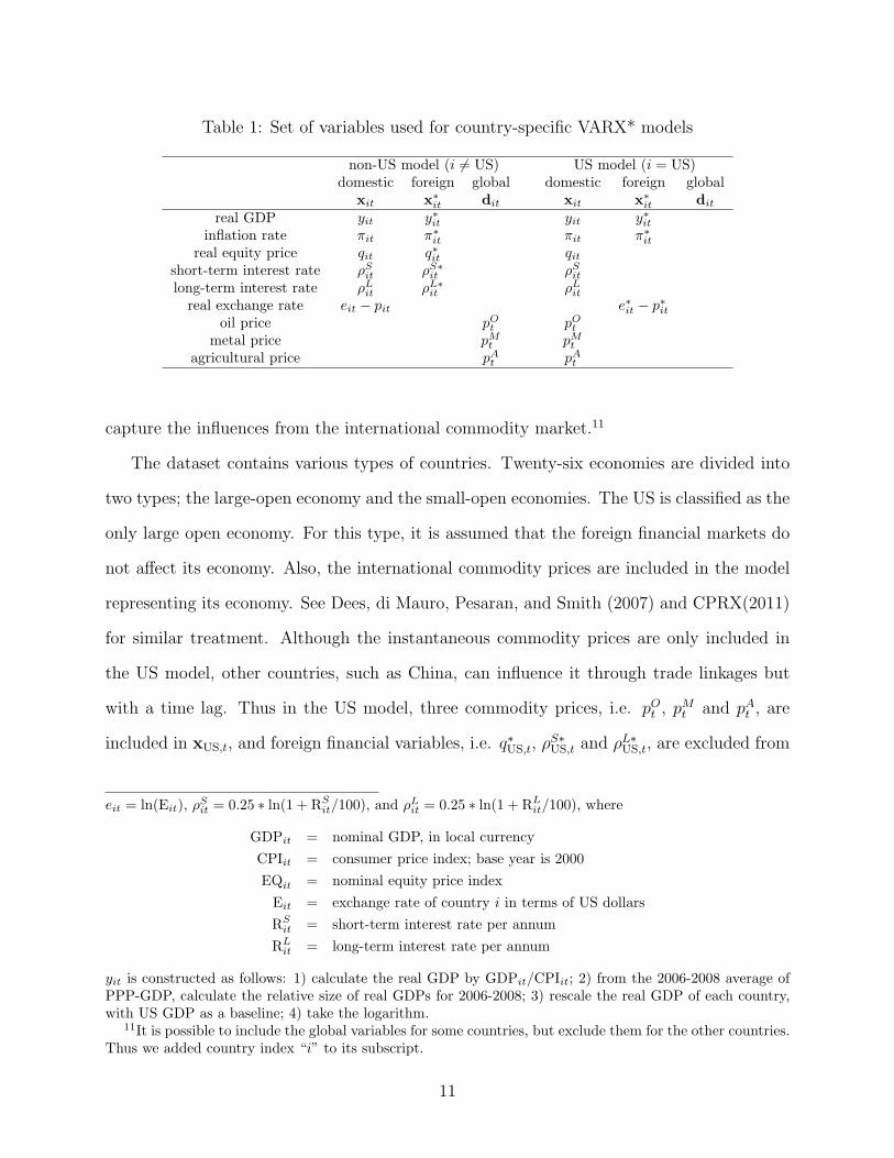
Table 1: Set of variables used for country-specific VARX* models
non-US model (i = US) US model (i = US)domestic foreign global domestic foreign global
xit x∗it dit xit x∗
it dit
real GDP yit y∗it yit y∗itinflation rate πit π∗
it πit π∗it
real equity price qit q∗it qitshort-term interest rate ρSit ρS∗
it ρSitlong-term interest rate ρLit ρL∗
it ρLitreal exchange rate eit − pit e∗it − p∗it
oil price pOt pOtmetal price pMt pMt
agricultural price pAt pAt
capture the influences from the international commodity market.11
The dataset contains various types of countries. Twenty-six economies are divided into
two types; the large-open economy and the small-open economies. The US is classified as the
only large open economy. For this type, it is assumed that the foreign financial markets do
not affect its economy. Also, the international commodity prices are included in the model
representing its economy. See Dees, di Mauro, Pesaran, and Smith (2007) and CPRX(2011)
for similar treatment. Although the instantaneous commodity prices are only included in
the US model, other countries, such as China, can influence it through trade linkages but
with a time lag. Thus in the US model, three commodity prices, i.e. pOt , pMt and pAt , are
included in xUS,t, and foreign financial variables, i.e. q∗US,t, ρS∗US,t and ρL∗US,t, are excluded from
eit = ln(Eit), ρSit = 0.25 ∗ ln(1 + RS
it/100), and ρLit = 0.25 ∗ ln(1 + RLit/100), where
GDPit = nominal GDP, in local currency
CPIit = consumer price index; base year is 2000
EQit = nominal equity price index
Eit = exchange rate of country i in terms of US dollars
RSit = short-term interest rate per annum
RLit = long-term interest rate per annum
yit is constructed as follows: 1) calculate the real GDP by GDPit/CPIit; 2) from the 2006-2008 average ofPPP-GDP, calculate the relative size of real GDPs for 2006-2008; 3) rescale the real GDP of each country,with US GDP as a baseline; 4) take the logarithm.
11It is possible to include the global variables for some countries, but exclude them for the other countries.Thus we added country index “i” to its subscript.
11
x∗US,t. This means that, for the US, the global variable dUS,t is empty.
For the rest of the sample economies, it is assumed that both the international commodity
markets and the foreign financial markets influence their economies. Thus for economy i,
three commodity prices are included in dit, and three foreign financial variables are included
in x∗it.
Lastly, regarding the real exchange rate, we include eit − pit in xit for the remaining
economies. However, conversely, it implies that the value of US currency is determined
outside the US economy, and thus e∗US,t − p∗US,t is treated as a part of a “US-specific foreign”
variable.
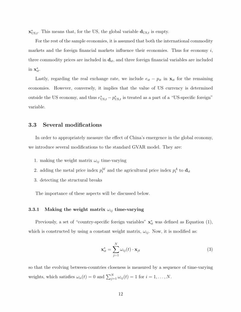
3.3 Several modifications
In order to appropriately measure the effect of China’s emergence in the global economy,
we introduce several modifications to the standard GVAR model. They are:
1. making the weight matrix ωij time-varying
2. adding the metal price index pMt and the agricultural price index pAt to dit
3. detecting the structural breaks
The importance of these aspects will be discussed below.
3.3.1 Making the weight matrix ωij time-varying
Previously, a set of “country-specific foreign variables” x∗it was defined as Equation (1),
which is constructed by using a constant weight matrix, ωij. Now, it is modified as:
x∗it =
N∑j=1
ωij(t) · xjt (3)
so that the evolving between-countries closeness is measured by a sequence of time-varying
weights, which satisfies ωii(t) = 0 and∑N
j=1 ωij(t) = 1 for i = 1, . . . , N .
12

To our best knowledge, the first published application of a time-varying weight matrix
was used by CPRX (2011), who investigated the impact of China’s economic growth on the
Latin American countries.
Since this weight represents the closeness of the economic activities between the countries,
the ideal weights should properly reflect this magnitude. In the literature of GVAR, either
one of two candidates is often used. One is the trade weight, which is constructed by using
the bi-directional trade flow data. The other is the financial weight, which represents the
flow of funds between the countries.
As we have examined in Section 2, China’s trade linkages with the rest of the world have
drastically increased after China joined the WTO in 2001. Although the financial linkages
are deepening, the trade linkages continue to define China’s economic impact. Besides, the
quality of data used for constructing the trade weight is more reliable than that of financial
weight, and these data are available from the 1980s.12 Thus we construct ωij(t) by using the
three-year averages of bi-directional trade flow data, obtained from the IMF’s Direction of
Trade Statistics.
3.3.2 Adding two commodity price indices
In the literature, the standard GVAR models are estimated with only one global variable,
i.e. the crude oil price, which is the representative of commodity “energy”. According to
Table 2, which reports the shares used for calculating the World Bank’s Commodity Price
Index, the share of crude oil in the energy index is 84.6%. The importance and the influence
of crude oil price fluctuations on the macroeconomic variables of countries, such as the US,
are reported by numerous researchers. Just to name a few, Hamilton (1983, 1996, 2003),
Hooker (1996), and Cunado and de Gracia (2005).
Besides “energy”, the World Bank publishes two more commodity indices, i.e. “non-
energy commodities” and “precious metals” (See Table 2); and the “non-energy commodi-
12For more discussion, see CPRX (2011).
13

Table 2: Shares used in the World Bank’s Commodity Price Index, in percentage
Commodity Share Commodity Share
Energy Non-energy CommoditiesCoal 4.7 Agriculture 64.9Crude Oil 84.6 Food 40.0Natural Gas 10.8 Others 24.8
Metals and Minerals 31.6Aluminum 8.4
Precious Metals Copper 12.1Gold 77.8 Iron Ore 6.0Silver 18.9 Others 5.1Platinum 3.3 Fertilizers 3.6Source: World Bank, Development Prospects Group. Based on 2002-04developing countries’ export values. November 24, 2008.
ties” group is further divided into “agriculture”, “metals and minerals”, and “fertilizers”.
The sum of “agriculture” and “metals and minerals” adds up to 96.5%. Since China is a
major importer of metals and agricultural products, it is worth investigating the importance
of including these indices in dit, which allows us to model the multiple channels of impact
propagation through the international commodity markets.
Table 3 summarizes the covariance analysis of three commodity prices (in log-differences).
The price of oil is the most volatile and the price of agricultural products is the least volatile.
In terms of the instantaneous correlation coefficients, Corr(∆pMt ,∆pAt ) = 0.5506 is the high-
est, Corr(∆pMt ,∆pOt ) = 0.4506 is the second highest, and Corr(∆pAt ,∆pOt ) = 0.3171 is the
lowest. It is often reported that both metals and agricultural products require a fair amount
of energy as an intermediate input. There is higher correlation between metals and oil, but
this is not supported by the correlation between agriculture and oil.
In order to further investigate the inter-variable relationship, a plain three-variate VAR
model is estimated for ∆pOt , ∆pAt , ∆pMt , and the causal relation is examined by the Granger
causality test. The optimal lag length of VAR, three, is selected by AIC. Table 4 reports
the results. The second column is the equation for “oil”, where the exclusion hypothesis of
“metal” is rejected at a 10% significance level. For the “agri” equation, neither “oil” nor
“metal” is a significant causal variable. Lastly, for the “metal” price, there is strong Granger
14

Table 3: Covariance analysis of three commodity price indices
Covariance Oil Agri Metal/Correlation ∆pOt ∆pAt ∆pMt
Oil 0.01991.0000
Agri 0.0022 0.00250.3171 1.0000
Metal 0.0061 0.0026 0.00910.4506 0.5506 1.0000
Note: pkt = ln(price index of commodity k) for k = O,A,M
Table 4: VAR Granger causality/Block exogeneity Wald tests
Dependent variableOil Agri Metal∆pOt ∆pAt ∆pMt
Oil 1.755 3.015Agri 4.881 20.808***Metal 7.479* 4.122All 15.155** 5.148 23.228***
Note: Three commodity prices are log-differenced. VAR(3) is used.***, **, *, represent 1 percent, 5 percent, and 10 percent significancelevels, respectively.
causality from the “agri” price. These results again contradict the view that “oil” is the
foremost intermediate input, so that a hike of the oil price increases both agricultural and
metal prices.
Given this preliminary analysis, we are now confident that the inclusion of agricultural
and metal prices provides additional information, which is not revealed by inclusion of only
oil prices.
3.3.3 Detecting the structural breaks with a difference-stationary VAR
As we formally report below, all the variables in our VARX* are the I(1) processes. Thus
if they are co-integrated, the VARX* model can be transformed into a vector error correction
model with exogenous variables. The previous papers in this field have mostly adopted this
specification, which makes us impose any long-run relations that might exist in the economy,
15

and increases the efficiency of parameter estimation.
However, as our sample covers the period between 1979Q1 and 2014Q3, it surely includes
influential events such as the Asian Financial Crisis in 1997, the Lehman Shock in 2008, etc.,
which are likely to generate the structural breaks. The difficulty of detecting the structural
break with the co-integrating VAR is reported by Hendry (2000).
A strand of research combines the Bayesian methods and the vector error correction
models (henceforth VECM). Jockmann and Koop (2011), for instance, have incorporated
the Markov switching into the VECM, which allows both the cointegrating vectors and the
number of cointegrating relationships to change when the regime changes. Even though it is
a fascinating approach, the computational burden outweighs the benefits when it is applied
to the GVAR.13 Besides, our aim is not forecasting but the historical evaluation of China’s
impact. Therefore, we treat the issue of structural breaks in a simpler manner.
First, the following “difference-stationary” VAR specification is used from now on:
∆xit = ai1 +
p−1∑k=1
Φik∆xi,t−k +
q−1∑ℓ=0
Λiℓ∆x∗i,t−ℓ +
r−1∑ℓ=0
Υiℓ∆di,t−ℓ + uit (4)
If it is correctly specified, the VECM is preferred to the difference-stationary VAR since the
former generates more efficient estimates. However, the presence of unpredictable structural
breaks hinders this task. Thus, we decided not to pursue the VECM specification.
Second, we have sequentially searched for one and only one significant “shift in intercept”
event for each equation, which is one form of a structural break, by t-test. For this purpose,
first, we search for the most significant intercept-shifts for each equation, by trimming the
both 20% edges of the sample period. After detecting the most significant intercept-shifts,
we add the intercept-shift dummy variables if and only if the intercept dummy is statistically
significant at a 5% level, to the model in order to control the effect of possible structural
breaks.
13As an application of the Markov switching VAR, Inoue and Okimoto (2008) investigated the effect ofJapanese monetary policy with hidden structural breaks. Using the difference-stationary VAR, they revealedthe existence, the timing, and the types of structural breaks in the monetary policy effects.
16
4 Estimation and testing
We proceed with the following analysis:
1. Testing the unit root
2. Detecting the structural breaks
3. Selecting the final specification of the models
4. Diagnostic tests
4.1 Testing the unit root
We begin by investigating the order of integration of each variable by using the Aug-
mented Dickey-Fuller Tests. The Akaike information criterion is used for selecting the opti-
mal lag length. The results indicate that most of the variables in levels contain a unit root,
but are stationary after a first differencing.
4.2 Detecting the structural breaks
The presence of structural breaks sometimes cast questions about the validity of the
estimated results. In the present case, any improper treatment of outliers might seriously
bias the shape of the impulse response functions. A fully flexible treatment of the structural
breaks should consider such aspects as: 1) the timing of the occurrence, 2) the number of
occurrences in the sample period, and 3) the types of changes, such as the intercept changes
and/or the slope changes in the regression context. For our current application, the full-
fledged treatment of the structural break is formidable due to the number of equations and
the number of variables in each equation. Thus our proposed treatment is quite conservative.
One remedy is to add an intercept-shift dummy variable, which is supposed to explain a
hidden dominant change of the data, if any. However, finding a good reason for adding such
dummies is also controversial. Besides, given a large number of equations, it is almost an
17

impossible task to examine such validities. Thus, ideally, we would like to detect and remove
intercept-shifts automatically.
More specifically, we have adopted the following steps to detect and remove the intercepts-
shifts.
1. Create a set of step-indicator dummy variables for the 20% to the 80% of the sample
period. Since our estimation period is 1980Q2 to 2014Q3, and the number of sample
period is T = 138, we have created approximately 80 step-indicator dummy variables;
2. Estimate the parameters of the GVAR model along with a step-indicator dummy one
at a time, and save the t-value of the step-indicator coefficient. Repeat this for all the
step-indicator dummy variables;
3. Choose the most significant step-indicator coefficient for each equation. If the t-value
is significant at a 5% level, then add the step-indicator dummy to the GVAR model.
Otherwise, discard.
This algorithm was run equation-by-equation with all the lag combination of p, q, and
r, and seven combinations of three commodity prices. In order to reduce the total number
of parameters, we restrict the maximum lag length of foreign variables, q, to two, and that
of global variables, r, to one. Further, we restrict the maximum lag lengths of domestic
variables, p, to three. The list of the detected outliers is stored, and used for selecting the
final specification for each country in the next step.
4.3 Selecting the final specification of the models
As the final step, adding the detected intercept dummy variable for each equation, we
re-estimate the country-specific VARX*(p, q, r) models. Given these estimates, we search
for the optimal lag lengths as well as the optimal combination of commodity prices for each
country by using the AIC. The results are shown in the left half of Table 5.
18

Table 5: Final specification of country-specific VARX*(p, q, r) models
p q r AIC selected p q r AICarg 3 1 1 707.4 O-M 3 1 1 706.4
austlia 3 1 1 2887.9 O-A-M 3 1 1 2878.3bra 3 2 1 903.5 M 3 2 1 902.5can 3 2 1 3209.2 O-M 3 2 1 3204.9
china 3 1 1 1850.3 A 3 1 1 1839.7chl 3 2 1 1577.8 O-A 3 1 1 1564.6
euro 2 1 1 3344.0 O-M 2 1 1 3335.2india 3 1 1 1905.4 M 3 1 1 1894.4indns 3 1 1 1295.4 A 3 1 1 1285.3japan 3 1 1 2945.9 A-M 3 1 1 2938.4kor 3 2 1 2558.9 A 3 2 1 2553.1mal 3 1 1 2043.7 O-A-M 3 1 1 2037.3mex 3 2 1 1366.2 O-A 3 2 1 1364.1nor 2 2 1 2743.8 O-A-M 2 1 1 2726.9nzld 3 2 1 2662.9 M 3 1 1 2657.5per 3 2 1 859.9 O-M 3 2 1 858.8phlp 3 1 1 1659.9 O-A 3 1 1 1659.4safrc 2 1 1 2650.3 O-A 2 1 1 2639.9sarbia 2 1 1 1443.1 O-A-M 2 1 1 1441.8sing 2 1 1 2100.5 O-A 2 1 1 2089.9swe 3 1 1 2826.8 O-A-M 3 1 1 2810.3
switz 3 2 1 3120.8 O-A 3 2 1 3112.2thai 2 1 1 1735.0 O-A 2 1 1 1729.3turk 3 2 1 1216.8 A 3 2 1 1214.6uk 2 1 1 3128.2 O-M 2 2 1 3120.7usa 3 1 na 3230.6 O-A-M 3 1 na 2817.1
3 commodity model Single commodity modelOil, Agri, & Metal Oil only
Note: Please refer to Table A1 in the Appendix for a glossary of acronyms. The specification used isEquation (4), where p=lag length of domestic variables (maximum lag is three), q=lag length of foreignvariables (maximum lag is two), and r=lag length of global variables(maximum lag is one). AIC = logL -(number of parameters). Each model includes at most one automatically detected intercept-shift dummy, atthe significance level of 5 percent. A column labelled “selected” reports the set of commodity prices includedin the final version of VARX* models, where O, A, and M means the oil, agriculture, and metal prices,respectively. For the US, the commodity prices are treated as its endogenous variables, thus the value of ris not available (na).
19

4.4 Diagnostic tests
The country-specific VARX*, Equation (4), includes the contemporaneous values of x∗it
and dit, on its right hand side. We investigate two issues relating to them in this subsection.
One is about the weak dependence of the idiosyncratic shocks, which is a key assumption
for the estimation of Equation (4). The second issue concerns the contemporaneous impact
of foreign variables on the domestic counterparts.
In the literature of GVAR, it is a common practice that the country-specific VARX*
models, Equation (4), i.e. the equations of xit, are estimated on a country-by-country basis.
As listed in Table 1, the commodity prices dit are part of xUS,t, even though they are treated
as exogenous in the small-open economies. Thus, Equation (4) specifies dynamics of the
domestic variables xit as well as the commodity prices dit. On the other hand, the dynamics
of x∗it is not estimated, but defined by Equation (3). Practically, this enables us to reduce
the number of parameters significantly, and make us construct the world model.
Three justifications for this estimation procedure are given by Pesaran, Schuermann, and
Weiner (2004). They are: 1) stability of the system; 2) smallness of weights ωij(t); and 3)
the weak dependence of the idiosyncratic shocks.14 Here, we examine the weak dependence
of the idiosyncratic shocks. Table 6 reports the average pair-wise cross-section correlations
for the levels and first differences of xit, as well as the associated VARX* residuals.
Generally speaking, the average pair-wise cross-section correlations are high for the “Lev-
els”, but they drop drastically as differenced. The correlations further decline as their dy-
namics are modeled by VARX*. A closer look reveals that the VARX* model with the
contemporaneous “star” variables (Type-2) generally yields much weaker dependence of id-
iosyncratic shocks than that without the contemporaneous “star” variables (Type-1). This
is consistent with the idea that the contemporaneous “star” variables function as proxies
for the common global factors. Thus, once country-specific models are formulated as being
14The stability of the system is numerically confirmed when the impulse response analysis is examined inthe latter section. The smallness of weights calculated from the trade flow data is reported elsewhere, thuswe do not repeat it. Concerning the weak dependence, see Appendix for additional discussion.
20

conditional on foreign variables, the remaining shocks across countries becomes weak, as
expected.
Next we examine the contemporaneous effects of foreign variables on their domestic
counterparts. Because the data are either log-differenced (for the real GDP, inflation, real
equity prices, and the exchange rate) or differenced (for two kinds of interest rates), one can
interpret the estimate as impact elasticity. Table 7 reports these estimates. The number of
asterisks indicates the level of statistical significance.
As for the statistically significant coefficients, all coefficients for short-term interest rates
are positive, as expected. For real output, the Asian countries are relatively less sensitive
to foreign demand since none of the coefficients is statistically significant even at a 10%
level. Concerning inflation, the significant foreign effects on Australia, China, Malaysia,
New Zealand and Singapore are observed. This might reflect the degree of openness of
these economies, however further investigation is needed. Noticeably, all the coefficients of
equity prices are positive and significant at the one percent level. For two interest rates,
similar phenomena are observed. The fact that the impact elasticities of equity prices and
the long-term interest rates exhibit highly significant coefficients might reflect the degree of
financial integration. On the other hand, the insensitivity of short-term interest rates for
several countries is due to their monetary policies. Except for Australia, New Zealand and
Singapore, the elasticities of short-term interest are insignificant for all the Asian countries.
5 Impulse response analysis
5.1 The Chinese impact
In this section, we estimate the GIRFs using the estimated GVAR model. The concept
of GIRFs was proposed by Koop, Pesaran, and Potter (1996) and has been applied to VAR
analysis by Pesaran and Shin (1998).
21

Table 6: Average pair-wise cross-section correlations of variables using in GVAR model andassociated model’s residuals
Levels 1st Diff Type-1 Type-2 Levels 1st Diff Type-1 Type-2 Levels 1st Diff Type-1 Type-2arg 0.91 0.08 -0.03 -0.02 0.29 0.05 0.06 0.03 0.46 0.23 0.15 -0.01
austlia 0.97 0.14 0.10 0.06 0.33 0.09 0.08 0.03 0.79 0.54 0.45 0.06bra 0.96 0.15 0.06 0.04 0.25 0.02 0.00 -0.05can 0.97 0.20 0.04 0.00 0.41 0.14 0.07 0.01 0.73 0.55 0.45 0.04
china 0.97 0.09 0.03 0.04 0.13 0.06 0.03 -0.01chl 0.97 0.14 0.05 0.05 0.39 0.05 0.04 0.03 0.77 0.34 0.33 0.08
euro 0.96 0.25 0.13 0.10 0.44 0.16 0.10 0.02 0.75 0.56 0.49 -0.09india 0.97 -0.02 -0.01 -0.01 0.16 0.04 0.05 0.04 0.76 0.32 0.25 0.02indns 0.97 0.10 0.01 0.01 0.03 0.05 0.04 0.03japan 0.89 0.15 0.05 0.05 0.35 0.09 0.05 0.05 0.29 0.44 0.28 -0.08kor 0.96 0.15 0.09 0.07 0.35 0.06 0.04 0.04 0.71 0.38 0.28 -0.03mal 0.97 0.20 0.06 0.05 0.26 0.11 0.08 0.04 0.62 0.40 0.37 0.04mex 0.97 0.16 0.06 0.04 0.23 0.00 0.03 0.02nor 0.96 0.09 0.06 0.05 0.37 0.08 0.06 0.02 0.80 0.50 0.39 0.08nzld 0.96 0.14 0.08 0.08 0.32 0.07 0.08 0.04 0.40 0.41 0.32 0.03per 0.88 0.06 0.02 0.02 0.26 -0.04 -0.02 -0.03
phlp 0.95 0.06 0.02 0.00 0.21 0.02 0.01 0.02 0.72 0.36 0.30 0.03safrc 0.95 0.19 0.07 0.07 0.33 0.04 0.02 0.01 0.77 0.47 0.38 0.10sarbia 0.91 0.03 0.04 0.03 -0.01 0.01 0.05 0.05sing 0.97 0.20 0.11 0.09 0.20 0.05 0.07 0.03 0.74 0.54 0.48 0.03swe 0.97 0.20 0.12 0.08 0.45 0.10 0.09 0.03 0.77 0.51 0.44 -0.01
switz 0.97 0.20 0.09 0.07 0.41 0.10 0.09 0.04 0.78 0.54 0.45 0.02thai 0.95 0.14 0.05 0.03 0.28 0.06 0.02 0.00 0.65 0.40 0.34 0.06turk 0.97 0.14 0.03 0.03 0.16 -0.01 0.00 -0.02uk 0.96 0.19 0.08 0.04 0.44 0.10 0.08 0.04 0.77 0.56 0.49 -0.01usa 0.97 0.21 0.09 0.04 0.40 0.18 0.08 0.01 0.77 0.54 0.43 -0.01
Levels 1st Diff Type-1 Type-2 Levels 1st Diff Type-1 Type-2 Levels 1st Diff Type-1 Type-2arg 0.37 0.09 0.05 0.04 0.45 0.03 0.05 0.01
austlia 0.83 0.37 0.23 0.22 0.62 0.13 0.12 0.05 0.89 0.38 0.30 0.04bra 0.79 0.21 0.11 0.10 0.43 0.01 0.04 -0.03can 0.81 0.32 0.15 0.13 0.67 0.18 0.14 0.11 0.91 0.36 0.31 -0.03
china 0.53 0.09 -0.01 -0.03 0.56 0.07 0.04 0.03chl 0.76 0.29 0.14 0.15 0.63 0.02 0.00 0.00
euro 0.80 0.35 0.24 0.25 0.68 0.17 0.10 0.06 0.89 0.44 0.34 -0.08india 0.61 0.26 0.12 0.10 0.30 0.10 0.07 0.06indns 0.35 0.22 0.12 0.12 0.26 0.07 0.06 0.05japan 0.72 0.16 0.11 0.11 0.62 0.03 0.02 0.02 0.86 0.26 0.21 -0.06kor 0.80 0.30 0.15 0.12 0.63 0.05 0.02 0.04 0.83 0.04 0.00 -0.05mal 0.76 0.30 0.17 0.15 0.50 0.06 0.02 0.05mex 0.73 0.10 0.01 0.00 0.52 0.02 0.03 0.03nor 0.82 0.39 0.24 0.24 0.63 0.05 0.00 -0.01 0.88 0.31 0.23 0.01nzld 0.83 0.37 0.23 0.21 0.59 0.06 0.08 0.02 0.81 0.19 0.11 0.03per 0.76 0.06 0.04 0.06 0.44 0.04 0.07 0.05
phlp 0.82 0.18 0.13 0.14 0.64 0.09 0.09 0.06safrc 0.71 0.32 0.18 0.17 0.54 0.11 0.06 0.04 0.68 0.21 0.14 0.01sarbia 0.67 0.08 0.04 0.04sing 0.83 0.38 0.24 0.24 0.60 0.08 0.07 0.04swe 0.78 0.35 0.21 0.20 0.70 0.09 0.04 0.01 0.91 0.40 0.31 0.04
switz 0.82 0.31 0.22 0.25 0.54 0.09 0.06 0.02 0.81 0.36 0.27 0.03thai 0.82 0.30 0.20 0.19 0.62 0.11 0.09 0.06turk 0.81 0.22 0.14 0.10 0.34 0.05 0.04 0.00uk 0.78 0.33 0.19 0.18 0.69 0.15 0.09 0.05 0.90 0.40 0.30 -0.02usa 0.62 0.10 0.06 0.04 0.88 0.40 0.33 -0.01
real exchange rate short-term interest rate long-term interest rateVARX* Res VARX* Res VARX* Res
real GDP inflation real equity pricesVARX* Res VARX* Res VARX* Res
Note: Please refer to Table A1 in the Appendix for a glossary of acronyms. VARX* Res (Type-2) refersto residuals from country-specific VARX* models. The specification is given as Equation (4). VARX* Res(Type-1) are obtained after re-estimating the model without the contemporaneous “star” variables.
22

Table 7: Contemporaneous effects of foreign variables on domestic counterparts by countries
arg 0.106 -1.701 1.095 *** 2.195austlia -0.007 0.625 ** 0.854 *** 0.468 *** 1.039 ***
bra 0.037 6.563 ** -5.525 *can 0.164 *** 0.677 *** 0.950 *** 0.524 *** 1.012 ***
china 0.096 0.403 * 0.015chl 0.071 0.091 0.762 *** 0.160 *
euro 0.090 * 0.203 ** 0.998 *** 0.065 *** 0.694 ***india 0.030 0.335 0.609 *** -0.045indns 0.114 -0.334 0.649japan -0.006 -0.202 0.638 *** -0.040 0.504 ***kor 0.026 0.359 0.988 *** -0.238 -0.069mal -0.012 0.447 * 1.350 *** -0.042mex 0.090 -0.770 0.764 **nor 0.099 0.642 1.071 *** 0.232 0.733 ***nzld 0.037 0.617 *** 0.729 *** 0.811 ** 0.439 **per -0.079 -1.065 0.483
phlp -0.044 -0.323 0.905 *** 0.395safrc 0.012 -0.074 0.813 *** 0.017 0.542 **sarbia 0.332 ** -0.033sing 0.087 0.419 ** 1.317 *** 0.293 *swe 0.399 *** 0.896 *** 1.117 *** 0.481 *** 0.907 ***
switz 0.114 0.581 *** 0.899 *** 0.245 *** 0.510 ***thai 0.059 0.294 0.870 *** 0.449turk -0.032 1.823 1.014 *uk 0.077 ** 0.396 ** 0.813 *** 0.242 ** 0.777 ***usa 0.143 *** 0.357 ***
real GDP inflation real equity prices short-term rate long-term rate
Note: Please refer to Table A1 in the Appendix for a glossary of acronyms. White’s heteroskedasticityrobust standard error is used. ***, **, *, represent 1 percent, 5 percent, and 10 percent significance levels,respectively.
Mathematically, it is defined as
GIRF(xt : uiℓt, n) = E[xt+n|uiℓt =
√σii,ℓℓ,Ωt−1
]− E
[xt+n|Ωt−1
](5)
where σii,ℓℓ is the corresponding diagonal element of the residuals’ variance-covariance matrix
Σu; Ωt−1 is the information set at time t− 1.
GIRFs are different from the standard IRFs proposed by Sims (1980), which assumes
orthogonal shocks. The standard IRFs are calculated using the Cholesky decomposition of
the covariance matrix of reduced-form errors. Thus, if we calculate the IRFs using different
orders of variables, the shape of the IRFs will be different. If a VAR contains two or three
variables, we might be able to use the standard IRFs by assuming a relation between the
variables inferred from economic theory. However, the same approach is not useful for the
GVAR model since it contains a large number of variables. This means that we cannot list a
23

Figure 3: GIRFs for a one percent decline in China’s GDP growth rate
-2.0
-1.6
-1.2
-0.8
-0.4
0.0
5 10 15 20
china
-.08-.07-.06-.05-.04-.03-.02-.01.00
5 10 15 20
usa
-.06
-.05
-.04
-.03
-.02
-.01
.00
5 10 15 20
euro
-.05
-.04
-.03
-.02
-.01
.00
5 10 15 20
japan
-.06-.05-.04-.03-.02-.01.00.01.02
5 10 15 20
aust lia
-.020
-.016
-.012
-.008
-.004
.000
5 10 15 20
india
-.12
-.10
-.08
-.06
-.04
-.02
.00
5 10 15 20
indns
-.08
-.06
-.04
-.02
.00
.02
.04
5 10 15 20
kor
-.06
-.05
-.04
-.03
-.02
-.01
.00
.01
5 10 15 20
mal
-.02
-.01
.00
.01
.02
.03
5 10 15 20
nzld
.000
.005
.010
.015
.020
.025
.030
.035
5 10 15 20
phlp
-.06-.05-.04-.03-.02-.01.00.01.02
5 10 15 20
s ing
-.10
-.08
-.06
-.04
-.02
.00
5 10 15 20
thai
-1.2
-1.0
-0.8
-0.6
-0.4
-0.2
0.0
5 10 15 20
oil
-.6
-.5
-.4
-.3
-.2
-.1
.0
5 10 15 20
agri
-1.4
-1.2
-1.0
-0.8
-0.6
-0.4
-0.2
0.0
5 10 15 20
metal
Note: Please refer to Table A1 in the Appendix for a glossary of acronyms. The lines correspond to theresponses of 1985(red dots), 1995(short dash), 2005(long dash), and 2013(line).
set of variables with a reasonable order that reflects economic theory. Therefore, instead of
using the standard IRFs proposed by Sims (1980), we use the GIRFs, which produce shock
response profiles that do not vary for different orders of variables.
We will investigate how a negative real GDP shock in China transmits to the Asian
countries as well as major developed economies based on the trade weights of 1985, 1995,
2005, and 2013. As explained in Section 2, as the trade linkages strengthen, we see a
significant shift in the trade weight matrices of 2005 and 2013 from those of 1985 and 1995.
Our focus is on seeing how the change of trade relations affects the propagation of shock.
First, we will examine the impact of a one percent drop in China’s real GDP growth rate
on the developed nations of the United States, the Eurozone, and Japan, see the first row
24

of Figure 3. The first panel shows the evolution of the Chinese GDP growth rate after a
one percent decline. Possibly due to the feedback effect, a one percent decline in the GDP
growth rate results in 1.6% reduction of the real GDP in levels after 20 quarters for China.
For the United States, the Eurozone, and Japan, the impact of a negative shock on Chinese
GDP is increasingly negative as we use more recent trade weights. However, the GIRFs have
a negative shape when using the trade weight matrices of 1985 and 1995, and these lines are
near zero. Therefore, it may imply that a negative Chinese shock would have had minimal
or nonexistent effect on these economies in 1985 and 1995.
In terms of the magnitude, we notice that the US experiences the most pronounced impact
compared to the Eurozone and Japan both in the short-term as well as the long-term. In
the long-term, the size of US GDP drops by 0.07%. On the other hand, for the Eurozone
and Japan, the size drops by approximately 0.05%. In terms of scale, the recent impact is
approximately 12 times bigger than that of 1985 for the US and the Eurozone. For Japan, it
is about 20 times bigger. Thus, we conclude that, over three decades, the US and Eurozone
exhibit similar responses both qualitatively and quantitatively. We will test the significance
of the negative impact in the next section.
The second to fourth rows of Figure 3 show the GIRFs for a one percent decline in China’s
growth on our set of Asian countries. As in the developed countries’ case, the impact of a
negative shock has become progressively negative on the Asian economies using more recent
trade weight structures. The Republic of Korea, Malaysia and Singapore had a nearly non-
existent impact with 1985 trade weight. Similar phenomena, but a slightly negative impact,
are observed for other countries.
Under more recent trade structures, every country except the Philippines experiences a
negative shock either in the short term or in the long term; however, the level and extent
of the shocks differ greatly. Indonesia is by far the most negatively impacted country both
in the short term as well as the long term. It is followed by Thailand (-0.095% in the
long term), the Republic of Korea (-0.070%), Singapore (-0.050%), Malaysia (-0.050%), and
25

Australia (-0.045%). The impact of a negative Chinese real GDP shock is less marked for
India (-0.018%). Interestingly, for the Philippines, the impact of a negative Chinese shock
is positive.
In the last three panels of Figure 3, we display the GIRFs for a one percent decline in
China’s GDP on three commodity price indices. China’s increasingly commodity-intensive
growth path manifests itself in the increasingly negative impact of Chinese negative growth
shock on commodity prices. Similar to the GIRFs observed above, the impact of Chinese
negative GDP shock is considerably more visible under the 2013 trade matrix structure.
China is the world’s largest consumer of industrial metals (-1.33% drop in a long term)
and the second-largest consumer of oil (-1.14%). China’s impact on agricultural prices rose
significantly after year 2000, although the impact on prices in both the short-term and the
long-term is much more muted compared to the impact on oil and metal prices.
Figure 4 shows the GIRFs for a one percent decline in China’s real GDP growth rate
using the trade weights of 2013 at a 68% confidence interval using a bootstrapping method.
The figures show that the GIRFs of US, Euro, Japan, Indonesia, the Republic of Korea,
Malaysia, Singapore and Thailand are significant at a 68% confidence interval.
Figure 5 compares the distribution of GIRFs with different trade weights. When we use
the trade weight matrix of 1985, the distribution of GIRFs stays close to the zero line for all
of the sample countries. However, with 2013 trade weights, we observe significant downward
shifts for the US, the Eurozone, Japan, Indonesia, Malaysia, Singapore and Thailand. For
Australia, India and the Republic of Korea, the dominant portion of the distribution has also
shifted downward. However, for the Philippines and New Zealand, the effect of a Chinese
shock is not very clear. We have summarized the patterns in Table 8.
Lastly, we also note that oil, metal and agricultural price indices are consistently all
negatively significant.
What is the response of other domestic variables? Figures 6 and 7 report the GIRFs of
three other variables, Dp (rate of inflation), eq (real equity price), and reer (real effective
26

Figure 4: Bootstrapped GIRFs for a one percent decline in China’s growth using the tradeweights of 2013
-2.4
-2.0
-1.6
-1.2
-0.8
-0.4
0.0
5 10 15 20
china
-.20
-.16
-.12
-.08
-.04
.00
5 10 15 20
usa
-.20
-.16
-.12
-.08
-.04
.00
5 10 15 20
euro
-.24
-.20
-.16
-.12
-.08
-.04
.00
5 10 15 20
japan
-.150-.125-.100-.075-.050-.025.000.025.050
5 10 15 20
austlia
-.07-.06-.05-.04-.03-.02-.01.00.01.02
5 10 15 20
india
-.35-.30-.25-.20-.15-.10-.05.00.05
5 10 15 20
indns
-.24-.20-.16-.12-.08-.04.00.04.08
5 10 15 20
kor
-.40-.35-.30-.25-.20-.15-.10-.05.00.05
5 10 15 20
mal
-.06
-.04
-.02
.00
.02
.04
.06
.08
5 10 15 20
nzld
-.12
-.08
-.04
.00
.04
.08
5 10 15 20
phlp
-.30-.25-.20-.15-.10-.05.00.05.10
5 10 15 20
sing
-.32-.28-.24-.20-.16-.12-.08-.04.00.04
5 10 15 20
thai
-3.2-2.8-2.4-2.0-1.6-1.2-0.8-0.40.0
5 10 15 20
oil
-1.6
-1.2
-0.8
-0.4
0.0
0.4
5 10 15 20
agri
-3.5
-3.0
-2.5
-2.0
-1.5
-1.0
-0.5
0.0
5 10 15 20
m etal
Note: Please refer to Table A1 in the Appendix for a glossary of acronyms. The lines correspond to the pathsof standard GIRF(blue), median(red line), and 16th and 84th percentiles (red long dash) of the distribution.
exchange rate). To make the figures concise and easier to understand, we have shortened
the horizontal axis from 21 quarters (five years) to 13 quarters (three years), and added two
vertical lines, corresponding to four quarters and eight quarters after the shock.
For the rate of inflation, it drops after a negative Chinese shock for all the countries,
except Indonesia. For the equity price, the markets of most countries are negatively impacted,
although there are notable differences. New Zealand is the only exception whose equity
market positively responds to a negative Chinese shock. As we have obtained a positive
response path for its real GDP, this might be the reason. Lastly, for the real effective
exchange rate, all countries experience depreciation.
27

Figure 5: 68 % bands of the GIRF distributions for different trade weights
-2.4
-2.0
-1.6
-1.2
-0.8
-0.4
0.0
5 10 15 20
china
-.20
-.16
-.12
-.08
-.04
.00
5 10 15 20
usa
-.20
-.16
-.12
-.08
-.04
.00
5 10 15 20
euro
-.24
-.20
-.16
-.12
-.08
-.04
.00
5 10 15 20
japan
-.150-.125-.100-.075-.050-.025.000.025.050
5 10 15 20
austlia
-.07-.06-.05-.04-.03-.02-.01.00.01.02
5 10 15 20
india
-.35-.30-.25-.20-.15-.10-.05.00.05
5 10 15 20
indns
-.24-.20-.16-.12-.08-.04.00.04.08
5 10 15 20
kor
-.40-.35-.30-.25-.20-.15-.10-.05.00.05
5 10 15 20
mal
-.06
-.04
-.02
.00
.02
.04
.06
.08
5 10 15 20
nzld
-.12
-.08
-.04
.00
.04
.08
5 10 15 20
phlp
-.30-.25-.20-.15-.10-.05.00.05.10
5 10 15 20
sing
-.32-.28-.24-.20-.16-.12-.08-.04.00.04
5 10 15 20
thai
Note: Please refer to Table A1 in the Appendix for a glossary of acronyms. The lines correspond to 16thand 84th percentiles of the distribution, calculated by the trade weights of 1985 (red dash), and that of 2013(blue line).
5.2 Further investigations
5.2.1 The impact of a potential US GDP shock
For comparison with the impact of a potential Chinese real GDP shock, analyzed in the
previous section, we will now investigate the impact of a one percent drop in US real GDP
on other countries. First, we review the GIRFs of China, the Eurozone, and Japan in Figure
8. Although the response of China with the trade weights of 2013 is found to be entirely
positive, which is quite counter-intuitive, the effect of the US on China becomes weaker over
the sample period.
On the other hand, for the Eurozone and Japan, we note that, although the impact is
28

Table 8: Classification of response patterns for the Asian countries with a one percent declinein China’s GDP growth rate
response patterns countriessignificantly lower japan, indns, mal, sing, thai
mostly lower austlia, india, korindeterminate nzld, phlp
Note: Please refer to Table A1 in the Appendix for a glossary of acronyms.
negative, the level and shape does not change across different trade matrices, which was the
case for China given its growing presence in the global economy.
Figure 8 shows that a decline of the US real GDP growth rate has a negative impact
on Asian countries, including New Zealand and the Philippines, which both showed a more
muted response to a Chinese shock. By comparing Figure 8 with Figure 3, it is easy to infer
that although the impact of a US shock will be considerably larger than a Chinese shock,
the magnitude of response progressively increases reflecting China’s increased economic ties
and influence on Asian economies.
In Figure 9, we calculated the 68% confidence interval using a bootstrapping method con-
trasting the GIRFs of 2013 and 1985. The impacts on the Republic of Korea and Singapore
are statistically significant at 68% confidence interval when using a trade weight matrix in
1985 and 2013. With the more recent trade structure, the response of Australia, Malaysia,
the Philippines, and Thailand also becomes statistically significant. For New Zealand, the
significant effect of the US is observed for four quarters after the shock. However, some
of the remaining countries show a borderline statistical significance, while others are not
statistically significant. In general, the distribution of GIRFs with respect to a one percent
decline in US ’s growth rate remains the same over the last three decades for the Asian
countries. This finding contrasts with the effect of a Chinese shock. Although the US has
a stronger influence on Asian economies than China, these countries are more exposed to
China than ever through increased economic ties.
29

Figure 6: Bootstrapped GIRFs for a one percent decline in China’s growth using the tradeweights of 2013
-2.4
-2.0
-1.6
-1.2
-0.8
-0.4
0.0
china
y
-.20
-.16
-.12
-.08
-.04
.00
usa
-.20
-.16
-.12
-.08
-.04
.00
euro
-.24
-.20
-.16
-.12
-.08
-.04
.00
japan
-.150-.125-.100-.075-.050-.025.000.025.050
austlia
-.07-.06-.05-.04-.03-.02-.01.00.01.02
india
-.5-.4-.3-.2-.1.0.1.2
dp
-.07-.06-.05-.04-.03-.02-.01.00.01.02
-.04
-.03
-.02
-.01
.00
.01
-.03
-.02
-.01
.00
.01
.02
-.08-.07-.06-.05-.04-.03-.02-.01.00.01
-.05
-.04
-.03
-.02
-.01
.00
.01
-1
0
1
eq
-.8
-.6
-.4
-.2
.0
.2
.4
-1.0-0.8-0.6-0.4-0.20.00.20.40.6
-2.0-1.6-1.2-0.8-0.40.00.40.8
-.8-.6-.4-.2.0.2.4.6.8
-1.2
-0.8
-0.4
0.0
0.4
0.8
-2.0
-1.6
-1.2
-0.8
-0.4
0.0
reer
-.8
-.6
-.4
-.2
.0
.2
.4
.0
.1
.2
.3
.4
.5
.6
-.4
-.2
.0
.2
.4
.6
-0.2
0.00.20.40.60.81.01.2
-.2
-.1
.0
.1
.2
.3
Note: Please refer to Table A1 in the Appendix for a glossary of acronyms. The lines correspond to thepath of median (blue), 16th and 84th percentiles (red dash) of the distribution. The horizontal axis is nowshortened to three years, and two vertical lines correspond to four quarters and eight quarters after theshock, respectively. For China’s equations, the real equity price is not included due to data unavailability.Thus the corresponding GIRFs are not calculated..
5.2.2 The shock propagations through metals and agricultural prices
Lastly, we re-examine the implication of adding two commodities to the standard GVAR
model. As we briefly discussed, in terms of AIC, we found the benefit of selecting the best
combinations out of three commodities over the oil-only model for all 26 economies.15 Here,
instead, we compare the shapes of the GIRFs using the year 2013 trade weights. See Figure
15We thank comments from Joseph Zveglich and Renee Fry-McKibbin on the treatment of this issue.
30

Figure 7: Bootstrapped GIRFs for a one percent decline in China’s growth using the tradeweights of 2013
-.30-.25-.20-.15-.10-.05.00.05
indns
y
-.24-.20-.16-.12-.08-.04.00.04.08
kor
-.36-.32-.28-.24-.20-.16-.12-.08-.04.00.04
mal
-.06-.04-.02.00.02.04.06.08
nzld
-.10-.08-.06-.04-.02.00.02.04.06.08
phlp
-.28-.24-.20-.16-.12-.08-.04.00.04.08
sing
-.32-.28-.24-.20-.16-.12-.08-.04.00.04
thai
.00
.04
.08
.12
.16
.20
dp
-.12-.10-.08-.06-.04-.02.00.02
-.12-.10-.08-.06-.04-.02.00.02.04
-.08-.06-.04-.02.00.02.04.06
-.10
-.08
-.06
-.04
-.02
.00
.02
-.06-.05-.04-.03-.02-.01.00.01
-.10-.08-.06-.04-.02.00.02.04
-1
0
1
eq
-3.0-2.5-2.0-1.5-1.0-0.50.00.51.0
-1.6-1.2-0.8-0.40.00.40.81.2
0.00.20.40.60.81.01.21.41.6
-2.0
-1.5
-1.0
-0.5
0.0
0.5
1.0
-1.6-1.2-0.8-0.40.00.40.81.2
-2.5-2.0-1.5-1.0-0.50.00.51.0
0.0
0.2
0.4
0.6
0.8
1.0
1.2
reer
-0.20.00.20.40.60.81.01.2
-.05.00.05.10.15.20.25.30.35
-.2-.1.0.1.2.3.4.5.6.7
-.3
-.2
-.1
.0
.1
.2
.3
-.12-.08-.04.00.04.08.12.16.20
-.3
-.2
-.1
.0
.1
.2
Note: Please refer to Table A1 in the Appendix for a glossary of acronyms. The lines correspond to thepath of median (blue), 16th and 84th percentiles (red dash) of the distribution. The horizontal axis is nowshortened to three years, and two vertical lines correspond to four quarters and eight quarters after the shock,respectively. For Indonesia’s equations, the real equity price is not included due to data unavailability. Thusthe corresponding GIRFs are not calculated.
10.16
The responses of the “oil-only” model appear to overestimate the impact of China’s
slowdown for the US, Australia, New Zealand, the Philippines, and Singapore. For example,
the response of Australia was significant with the “oil-only” model, which now becomes
marginally insignificant with three-commodity model. According to Table 5, the VARX*
model of Australia includes all three commodity prices. This suggests the usefulness of
adding two commodity prices to the GVAR model. On the other hand, for Indonesia, the
16For Argentina and Chile, the VARX* lags selected by the AIC were p = 3, q = 2, and r = 1, or(3,2,1). However, when the GIRFs are calculated, we could not obtain the stable solutions with them. Afterexamining the AICs for different combinations of lags for all the countries, we noticed that the incrementsof AIC for Argentina and Chile from (3,1,1) to (3,2,1) were almost negligible. Thus we impose (3,1,1) forthese two countries. Figure 10 is calculated under these restrictions.
31

Figure 8: GIRFs for a one percent decline in US’s GDP growth rate
-.12
-.08
-.04
.00
.04
.08
.12
5 10 15 20
china
-2.0
-1.6
-1.2
-0.8
-0.4
0.0
5 10 15 20
usa
-.5
-.4
-.3
-.2
-.1
.0
5 10 15 20
euro
-.6
-.5
-.4
-.3
-.2
-.1
.0
5 10 15 20
japan
-.28
-.24
-.20
-.16
-.12
-.08
-.04
.00
5 10 15 20
aust lia
-.12
-.08
-.04
.00
.04
.08
5 10 15 20
india
-.40-.35-.30-.25-.20-.15-.10-.05.00
5 10 15 20
indns
-.8-.7-.6-.5-.4-.3-.2-.1.0
5 10 15 20
kor
-.9-.8-.7-.6-.5-.4-.3-.2-.1.0
5 10 15 20
mal
-.24
-.20
-.16
-.12
-.08
-.04
.00
5 10 15 20
nzld
-.5
-.4
-.3
-.2
-.1
.0
5 10 15 20
phlp
-.9-.8-.7-.6-.5-.4-.3-.2-.1.0
5 10 15 20
s ing
-.6
-.5
-.4
-.3
-.2
-.1
.0
5 10 15 20
thai
-9-8-7-6-5-4-3-2-10
5 10 15 20
oil
-3.5
-3.0
-2.5
-2.0
-1.5
-1.0
-0.5
0.0
5 10 15 20
agri
-12
-10
-8
-6
-4
-2
0
5 10 15 20
metal
Note: Please refer to Table A1 in the Appendix for a glossary of acronyms. The lines correspond to theresponses of 1985(red dots), 1995(short dash), 2005(long dash), and 2013(line).
three commodities model suggests a larger negative impact in the long-term. Although the
magnitude is much smaller than that of Indonesia, the negative impact of a Chinese shock on
Malaysia and Thailand are also larger with three commodity models. These results indicate
the usefulness of including the multiple commodity prices in order to capture the different
channels of shock transmission.
6 Conclusions and remarks
In this paper, following CPRX, we estimated a GVAR model using a time-varying trade
weight matrix. China’s economy has been growing fast and its presence in the global economy
32

Figure 9: 68 % bands of the GIRF distributions for different trade weights
-.4
-.3
-.2
-.1
.0
.1
.2
.3
5 10 15 20
china
-2.4
-2.0
-1.6
-1.2
-0.8
-0.4
0.0
5 10 15 20
usa
-.9-.8-.7-.6-.5-.4-.3-.2-.1.0
5 10 15 20
euro
-1.2
-1.0
-0.8
-0.6
-0.4
-0.2
0.0
0.2
5 10 15 20
japan
-.6
-.5
-.4
-.3
-.2
-.1
.0
.1
5 10 15 20
aust lia
-.4
-.3
-.2
-.1
.0
.1
5 10 15 20
india
-1.2
-1.0
-0.8
-0.6
-0.4
-0.2
0.0
0.2
5 10 15 20
indns
-1.4-1.2-1.0-0.8-0.6-0.4-0.20.00.2
5 10 15 20
kor
-2.0
-1.6
-1.2
-0.8
-0.4
0.0
0.4
5 10 15 20
mal
-.4
-.3
-.2
-.1
.0
.1
.2
.3
5 10 15 20
nzld
-1.0
-0.8
-0.6
-0.4
-0.2
0.0
0.2
5 10 15 20
phlp
-2.0
-1.6
-1.2
-0.8
-0.4
0.0
5 10 15 20
s ing
-1.4-1.2-1.0-0.8-0.6-0.4-0.20.00.2
5 10 15 20
thai
Note: Please refer to Table A1 in the Appendix for a glossary of acronyms. The lines correspond to 16thand 84th percentiles of the distribution, calculated by the trade weights of 1985 (red dash), and that of 2013(blue line).
is expanding through trade relations. We analyzed how and to what extent the Chinese
economic fluctuations affect the global economy – the Asia Pacific region in particular. After
estimating the GVAR model, we calculated the GIRFs with different trade weight matrices of
1985, 1995, 2005, and 2013 in order to compare the size and timing of the shock propagations.
We also calculated the 68% and 90% confidence intervals using the bootstrapping method
and tested whether the estimated impacts are statistically significant.
Unlike under the earlier trade structures of 1985 or 1995, a negative shock to the Chinese
real GDP has a significant impact on the surrounding countries under the more recent trade
structures of 2005 or 2013. When we evaluated the impact using the trade weights of 2013, we
found that a negative Chinese GDP shock impacts commodity exporters, such as Indonesia,
33

Figure 10: GIRFs for a one percent decline in China’s GDP growth rate with and withoutfull set of commodities
-2.4
-2.0
-1.6
-1.2
-0.8
-0.4
0.0
5 10 15 20
china
-.24
-.20
-.16
-.12
-.08
-.04
.00
5 10 15 20
usa
-.24
-.20
-.16
-.12
-.08
-.04
.00
5 10 15 20
euro
-.24
-.20
-.16
-.12
-.08
-.04
.00
5 10 15 20
japan
-.20
-.15
-.10
-.05
.00
.05
5 10 15 20
aust lia
-.07-.06-.05-.04-.03-.02-.01.00.01.02
5 10 15 20
india
-.35-.30-.25-.20-.15-.10-.05.00.05
5 10 15 20
indns
-.30-.25-.20-.15-.10-.05.00.05.10
5 10 15 20
kor
-.40-.35-.30-.25-.20-.15-.10-.05.00.05
5 10 15 20
mal
-.08-.06-.04-.02.00.02.04.06.08
5 10 15 20
nzld
-.16
-.12
-.08
-.04
.00
.04
.08
5 10 15 20
phlp
-.4
-.3
-.2
-.1
.0
.1
5 10 15 20
s ing
-.32-.28-.24-.20-.16-.12-.08-.04.00.04
5 10 15 20
thai
Note: Please refer to Table A1 in the Appendix for a glossary of acronyms. The lines correspond to the 16thand 84th percentiles of the “oil-only” case(red dots) and the “optimal combination of multiple commodities”case (blue line)
the most, reflecting both demand and terms of trade shocks. Export-dependent countries
on the East Asian production cycle, such as Japan, Singapore, Malaysia and Thailand, are
also severely affected.
A shock to the Chinese real GDP also has an impact on the international prices of not
only the crude oil market but also metals and agricultural markets, showing the degree of
influence of China on the global terms of trade.
With regard to the future research, we consider improvement of the trade weight matrix
to be the key. In this paper, following CPRX, we used the trade weight matrix representing
the linkages to different countries. However, capital inflows and outflows significantly affect
34

Table A1: Country Abbreviations
Name Short name Name Short name
Argentina arg Norway norAustralia austlia New Zealand nzldBrazil bra Peru perCanada can Philippines phlpChina china South Africa safrcChile chl Saudi Arabia sarbiaEurozone euro Singapore singIndia india Sweden sweIndonesia indns Switzerland switzJapan japan Thailand thaiKorea kor Turkey turkMalaysia mal United Kingdom ukMexico mex USA usaNote) “Eurozone” includes Austria, Belgium, Finland, France, Germany, Italy,Netherlands, and Spain.
economies. Since the measurement of closeness of countries is key for the GVAR model, we
should also consider using foreign direct investment data. If we can capture the financial
linkages between countries, we can, for example, analyze the impact of monetary policy
changes in advanced economies on developing countries.
Appendix
Data
We obtained the data files that cover the period between 1979Q1 and 2011Q2 from the“The GVAR toolbox” website at Centre for Financial Analysis & Policy, Judge BusinessSchool, University of Cambridge.17 We have added the recent data for the period between2011Q3 and 2014Q3 mainly based on Appendix B in Smith and Gales (2011). We usedthe World Bank’s commodity price data downloaded from the following website.18 We havereplaced Smith’s oil price data with the World Bank’s index, and added the metal index andagriculture index. The more detailed information about the added data is available from theauthors upon request.
17URL is http://www.cfap.jbs.cam.ac.uk/research/gvartoolbox/download.html.18URL is http://econ.worldbank.org/WBSITE/EXTERNAL/EXTDEC/EXTDECPROSPECTS/0,,contentMDK:
21574907 menuPK:7859231 pagePK:64165401 piPK:64165026 theSitePK:476883,00.html
35

On the weak exogeneity
This subsection follows the example by Fisher (1993) with a slight modification. Forsimplicity, let both xt and x∗
t be scalars, and consider the VAR* model for a country (withoutcountry index i) [
∆xt
∆x∗t
]=
[a1
a2
]+
[Γ11 Γ12
Γ21 Γ22
] [∆xt−1
∆x∗t−1
]+
[u1t
u2t
](6)
One can reparameterize Equation (6) in terms of conditional and marginal models as:
∆xt = θ0 + θ1∆x∗t + θ2∆xt−1 + θ3∆x∗
t−1 + ζt (7)
∆x∗t = a2 + Γ21∆xt−1 + Γ22∆x∗
t−1 + u2t (8)
The error term of the conditional model becomes:
ζt ≡ u1t − θ1u2t ∼ N(0,Ω)
where Ω = Σ11 − Σ12Σ−122 Σ21 with Σs being the corresponding covariance elements of
(u′1t,u
′2t)
′. Then, the parameters in Equations (6), (7), and (8) are related as:
θ1 = Σ12Σ−122 , θ0 = a1 − θ1a2, θ2 = Γ11 − θ1Γ21, θ3 = Γ21 − θ1Γ22.
The short-run dynamic stability of the conditional model requires θ2 in Equation (7) to be|θ2| < 1. If this restriction is not imposed, the parameters of the conditional distributionλ1 = (θ0, θ1, θ2, θ3,Ω) and marginal distributions λ2 = (a2,Γ21,Γ22,Σ22) define a sequentialcut between the conditional and the marginal models. Hence, weak exogeneity holds.
If the short-run dynamic stability is imposed, on the other hand, it implies |Γ11−θ1Γ21| <1 due to cross-equation restrictions. Under this circumstance, λ1 and λ2 are no longervariation free. However, if Γ21 is zero, weak exogeneity still holds.
Following this insight, we have investigated the weak dependence of idiosyncratic shocks,and confirmed that pair-wise cross-section correlations of shocks are actually very weak.
References
Ahuja, A. and A. Myrvoda (2012).“The Spillover Effects of a Downturn in China’s RealEstate Investment,” IMF Working Paper, WP/12/266.
Ahuja, A. and M. Nabar (2012). “Investment-Led Growth in China: Global Spillovers,” IMFWorking Paper, WP/12/267.
Caporale, G., M., and A. Girardi (2013). “Fiscal spillovers in the Euro area,” Journal ofInternational Money and Finance, 38 84, e1-e16.
Cesa-Bianchi, A., M. H. Pesaran, A. Rebucci, and T. Xu (2011). “China’s Emergence in theWorld Economy and Business Cycles in Latin America,” IDB Working Paper Series No.IDB-WP-266.
36

Chen, Q., D. Gray, P. N’ Diaye, H. Oura, and N. Tamirisa (2010). “International Transmis-sion of Bank and Corporate Distress,” IMF Working Paper WP/10/124.
Chudik, A., and M. Fratzscher (2011). “Identifying the global transmission of the 2007-2009financial crisis in a GVAR model,” European Economic Review, 55, 325-339.
Chudik, A., and M. H. Pesaran (2014). “Theory and Practice of GVAR Modeling,” FederalReserve Bank of Dallas Working Paper, No. 180.
Cunado, J. and F.P. de Gracia (2005). “Oil prices, Economic Activity and Inflation: Evidencefor Some Asian Countries,” The Quarterly Review of Economics and Finance, Volume 45,Issue 1, 65-83.
Dees S, di Mauro F, Pesaran MH, Smith LV (2007). “Exploring the International Linkagesof the Euro Area: a Global VAR Analysis,” Journal of Applied Econometrics, 22, 1-38.
Dees S, Holly S, Pesaran MH, Smith LV (2007). “Long-Run Macroeconomic Relations in theGlobal Economy,” Economics: The Open-Access, Open-Assessment E-Journal 3, 1-56.
Duval, R., K. Cheng, K.H. Oh, and R. Saraf (2014). “Trade Integration and Business CycleSynchronization: A Reappraisal with Focus on Asia,” IMF Working Paper, WP/14/52.
Eickmeier, S., and T. Ng (2015). “How do US credit supply shocks propagate internationally?A GVAR approach,” European Economic Review, 74, 128-145.
Favero, A. (2013). “Modelling and forecasting government bond spreads in the euro area: aGVAR model”, Journal of Econometrics, 177, 2, 343-356.
Fischer, Andreas M. (1993). “Weak Exogeneity and Dynamic Stability in CointegratedVARs,” Economics Letters, Volume 43, Issue 2, 167-170.
Gray,D., M.Gross, J.Paredes, and M. Sydow (2013). “Modeling Banking, Sovereign, andMacro Risk in a CCA Global VAR,” IMF Working Paper, WP/13/218.
Koop, G., M. H. Pesaran, and S. M. Potter (1996). “Impulse Response Analysis in NonlinearMultivariate Models,” Journal of Econometrics, 74(1) 119-147.
Hamilton, J. (1983). “Oil and the Macroeconomy Since World War II,” Journal of PoliticalEconomy, 228-248.
Hamilton, J. (1996). “This is What Happened to the Oil Price-Macroeconomy Relationship,”Journal of Monetary Economics, Volume 38, Issue 2, 215-220.
Hamilton, J. (2003). “What is an Oil Shock?,” Journal of Econometrics, Volume 113, Issue2, 363-398.
Han, F., and T. H. Ng (2011). “ASEAN-5 Macroeconomic Forecasting Using a GVARModel,” ADB Working Paper Series on Regional Economic Integration No.76.
37

Hendry, D.F. (2000). “On Detectable and Non-detectable Structural Change,” StructuralChange and Economic Dynamics, Volume 11, Issues 1-2, 45-65.
Hiebert, P. and I. Vansteenkiste (2010). “International trade, technological shocks andspillovers in the labour market : a GVAR analysis of the US manufacturing sector,” Appliedeconomics, Vol. 42, 22/24, 3045-3066.
Hooker, M. (1996). “What Happened to the Oil Price-Macroeconomy Relationship?,” Jour-nal of Monetary Economics, Volume 38, Issue 2, 195-213.
IMF Country Report (2011). “People’s Republic of China: 2011 Spillover Report - SelectedIssues,” June 28, 2011. http://www.imf.org/external/pubs/ft/scr/2011/cr11193.pdf.
Inoue, T. and T. Okimoto (2008). “Were There Structural Breaks in the Effect of JapaneseMonetary Policy?: Re-evaluating the Policy Effects of the Lost Decade,” Journal of theJapanese and International Economies 22(3), 320-342.
Jockmann, M. and G. Koop (2011). “Regime-Switching Cointegration,” mimeo, May 2011.http://personal.strath.ac.uk/gary.koop/jochmann koop 2011.pdf.
Matsubayashi, Y. (2013). “Deepening of International Interdependence and the EastAsian Economy: Empirical Evidence based on Global VAR,” in Impacts thatthe Structural Transformation of the World Economy Has on the East Asian Re-gion (Report of Joint International Research Project by Japan, China and Ko-rea), Economic and Social Research Institute, Cabinet Office, Government of Japan.http://www.esri.go.jp/jp/prj/int prj/2013/prj2013 01 05e.pdf.
Pesaran, M.H., T. Schuermann, and S.M. Weiner (2004). “Modeling Regional Interdepen-dencies Using a Global Error-Correcting Macroeconometric Model,” Journal of Business andEconomic Statitics, 22, 129-162.
Pesaran, M. H., and Y. Shin (1998). “Generalized Impulse Response Analysis in LinearMultivariate Model,” Economics Letters, 58(1), 17-29.
Pesaran, M. H., Y. Shin, and R. J. Smith (2000). “Structural Analysis of Vector ErrorCorrection Models with Exogenous I(1) Variables,” Journal of Econometrics, 97(2), 293-343.
Smith, L., V. and A. Galesi (2011). “GVAR Toolbox 1.1” mimeo.http://www-cfap.jbs.cam.ac.uk/research/gvartoolbox/index.html.
Sims, C. (1980). “Macroeconomics and Reality,” Econometrica, 48, 1-48.
Vansteenkiste, I. (2007). “Regional Housing Market Spillovers in the US: Lessons from Re-gional Divergences in a Common Monetary Policy Setting,” ECB Working Paper No.708.
38