The Impact of Benchmarkingin Fixed Income Markets

Giorgio Ottonello*

This Version: September 26, 2019

Abstract

I empirically study the asset pricing implications of corporate bond funds’ performanceconcerns relative to a benchmark index. Benchmarking has a large impact on bondprices, as funds re-balance in response to mechanical index weight changes. On average,a long/short portfolio of bonds with a mechanical increase/decrease in index weightsgenerates a monthly alpha of 40 bps. The direction and magnitude of this effect dependon past flows and cash levels of both passive and active funds holding the assets. Overall,the design of fixed income benchmarks distorts the portfolio allocation of all bond funds,ultimately affecting the pricing of corporate bonds beyond fundamentals.

JEL-Classification: G12, G23Keywords: US corporate bond market, benchmarking, institutional investors

*Vienna Graduate School of Finance (VGSF), Building D4, 4th floor, Welthandelsplatz 1, 1020 Vienna,Austria; email: giorgio.ottonello@wu.ac.at

First Version: March 31, 2018I would like to thank Maximilian Bredendiek, Matthijs Breugem, Andrea M. Buffa, Adrian Buss, GiovanniCespa, Jaewon Choi, Jens Dick-Nielsenm, Bernard Dumas, Richard Evans, Miguel Ferreira, Peter Feldhut-ter, Javier Gil-Bazo, Thierry Focault, Johan Hombert, Matti Keloharju, Rainer Jankowitsch, Christian Laux,David Lando, Pab Jotikasthira, Florian Nagler, Anthony Neuberger, Roberto Pinto, Vesa Puttonen, ChristophScheuch, Sean Seunghun Shin, Marti G. Subrahamanyam, Allan Timmermann, Davide Tomio, Rossen Valka-nov, Kumar Venkataram, Christian Wagner and Josef Zechner for helpful comments and suggestions. I alsowould like to thank seminar and conference participants at Erasmus School of Economics, Aalto, CBS, NOVA,HEC Paris, Collegio Carlo Alberto, BI Oslo, Cass Business School, ESADE, UPF, SMU Cox School of Busi-ness, Vienna Graduate School of Finance (VGSF), the Rady School of Management at UCSD, and the DardenSchool of Business. Part of this research was completed when I was a visiting PhD student at NYU Stern.I gratefully acknowledge financial support from FWF (Austrian Science Fund) DOC 23-G16. Any remainingerrors are my own.

1 Introduction

Open end mutual funds are key players in financial markets, with $40 trillion under

management globally in 2016. The performance of most active and passive fund managers

is evaluated against a benchmark index, either through explicit compensation or indirectly,

through the flow-to-performance relation.1 Recent papers show that benchmarking incentives

affect institutions’ trading strategies and distort prices in equity markets.2

The growing industry of corporate bond funds is evaluated against benchmarks which are

much different from stock indexes.3 Fixed-income benchmarks include many more assets,

while also having a larger and more frequent turnover. Additionally, index constituents are

less liquid, as corporate bonds are traded Over-the-Counter (OTC).4 Whether benchmarking

impacts portfolio allocation in fixed income funds and hence bond prices, is an open issue. If

it does, are the effects related to mutual funds’ liquidity management? Bond funds allow daily

redemptions like equity funds, but differently from them hold illiquid assets. Such liquidity

mismatch sparked a discussion on whether bond funds are exposed to runs.5 Shedding light

on the drivers of portfolio allocation of bond funds is a key contribution to the debate.

My paper tackles these questions by empirically studying the asset pricing implications

of benchmarking incentives in the US corporate bond market, and how they relate to funds’

liquidity management. First, I find that benchmarking has a large impact on corporate bond

prices, as funds re-balance in response to mechanical weight changes in the benchmark index.

On average, a long/short portfolio of bonds with index weight increases/decreases generates

an α of 40 bps per month. Second, I show that the direction and magnitude of the price

impacts critically depend on past flows and cash levels of both the active and passive bond

funds holding the assets. Third, I provide evidence that the documented impact gets larger

when a higher fraction of the institutions in the market are benchmarked. My findings show

1For example, in 2017 $16 trillion in assets were benchmarked to indexes offered by FTSE Russell.2See Basak and Pavlova (2013), Chen, Noronha, and Singal (2005), Chang, Hong, and Liskovich (2015).3AUM (investment in corporate bonds) from $1.5 ($0.52) trillion in 2008, to $3.6 ($1.6) trillion in 2016.4These features do not allow bond funds to hold the index, and leads them to invest into a subset of it.5See Goldstein, Jiang, and Ng (2017) and Zeng (2017).

1

that benchmarking is an important channel through which institutional investors affect the

pricing of corporate bonds beyond fundamentals.

To guide my empirical tests, I propose a theoretically motivated re-balancing mechanism

for bond funds in response to index weight changes. The mechanism works as follows. Risk-

averse fund managers trade-off hedging demand for illiquid assets in the benchmark against

holding cash in expectation of future redemptions.6 Consider a fund manager with a portfolio

of illiquid index assets and cash, facing unexpected changes in the benchmark. While the

hedging demand changes proportionally to the variation in the index weights, the total effect

on the portfolio allocation depends on the net fund flows. All else equal, if the fund experiences

net inflows, the manager has additional cash to re-invest, which increases her demand for risky

assets. Overall, the manager will buy more assets that increased the index weight and sell

fewer of those that decreased it. If the liquidity discounts are large enough, the manager

could end up only investing the inflows in bonds with weight increases, avoiding selling those

with decreases. On the other hand, after meeting large redemptions, the manager will rebuild

her cash holdings in expectation of future outflows.7 In aggregate, the manager will sell more

assets that decreased the index weight and buy fewer of those that increased it. The cash

rebuilding motive can push the manager to sell more than what she would sell in a liquid

market (e.g. equities). Intuitively, the aggregate amount of re-balancing and its effect on

bond prices increases when a larger fraction of investors in the market is benchmarked.

In my empirical analysis, I use Bank of America/Merrill Lynch (BofA/ML) US High Yield

Index and BofA/ML US Corporate Index monthly changes in constituents’ weights as shocks

to benchmarked investors’ hedging demand. Using a sample from November 2004 to June

2016, I sort corporate bonds based on past index weight changes into quintile portfolios on a

monthly basis, and analyze equally-weighted excess returns. First, I investigate the average

6The corporate bond market is illiquid due to its OTC structure. Trading an asset might lead to largediscounts. Hence, in order to limit expected liquidation costs arising from future redemptions, managers holdlarger cash buffers than what they would keep in a liquid market (e.g. equity funds). See Chermenko andSunderam (2016), Choi and Shin (2018), Goldstein, Jiang, and Ng (2017).

7See Zeng (2017) for a detailed analysis of the cash rebuilding mechanism in a dynamic model.

2

effect across all assets. Going long into the bonds with the most positive index weight changes

and short into those with the most negative, earns an average monthly excess returns of 39.87

bps, generating an α of 39.5 bps beyond stock and bond pricing factors. For high yield (HY)

(investment grade, [IG]) bonds, the excess return is 88.97 (14.77) bps, with an α of 88.10

bps (13.43 bps). Importantly, the price effects are not coming from a symmetric reaction

to positive and negative index weight changes. Bonds with large weight increases generate

positive excess returns, while those with decreases show no drop in prices. Bonds in my

sample are on average exposed to positive flows. Hence, my result is consistent with funds

re-investing inflows and buying assets that increased the index weight while selling fewer of

those that decreased it.

I rule out several alternative explanations. First, my findings are not driven by weight

changes linked to variations in a bond’s fundamental value, which are excluded from the

sample.8 Second, they are robust to multiple regression specifications wherein I control for

bond characteristics, fund flows, past performance and time-issuer fixed effects. Third, I

provide evidence that my findings cannot be explained by past month returns (i.e., institutions

persistently buying bonds that performed best in the previous month). Fourth, the effects

I document are unchanged when using value-weighted portfolio returns or including in the

sample index inclusions and exclusions.

In an attempt to pin down the interaction between benchmarking and liquidity manage-

ment in bond funds, I study how the price distortions relate to different levels of past fund

flows. I do so by constructing a measure of bond-specific exposure to fund flows. In line with

the cash rebuilding mechanism, I find that, after being exposed to large outflows, bonds with

index weight decreases are sold more than those with weight increases are bought. This leads

to large negative price impacts on the bonds that had the most negative index weight changes,

up to an average of −57.56 bps excess monthly returns. Consistent with the reinvestment

8I do not consider bonds that enter/exit the index, or those that experience any rating change. Indexinclusions and exclusions are events that are easy to predict, and could be mixed with other trading motives.Rating changes reflect a variation in credit risk, which is linked to the fundamental value of the bond.

3

channel, bonds exposed to inflows present instead stronger impacts (positive excess returns

and excess buying activity) on assets with the most positive weight changes. The magnitudes

of the effects are larger in the HY segment, where flows of active funds seem to be the main

driver. In the IG segment, however, flows of index funds play a dominant role.

In addition, I focus on bonds exposed to outflows, and study how the price distortions vary

according to the level of funds’ cash holdings. In this case, I construct a measure of bond-

specific exposure to fund cash holdings. Intuitively, I find that bonds exposed to high cash

holdings exhibit effects in line with the reinvestment channel. Interestingly, bonds exposed to

low cash holdings present price impacts that are consistent with cash rebuilding, with negative

returns on the assets affected by index weight decreases. Taken together, my findings on flows

and cash levels point at relative performance concerns as a potential channel for instability

in fixed income markets. If many funds with low cash holdings are hit by large outflows at

the same time, benchmarked asset managers will try to rebuild their cash buffer by selling

the same assets. This could lead to widespread fire-sales and potentially more outflows and

fund distress.

I provide evidence that the price impacts following index changes come indeed from bench-

marked institutions. I analyze quarterly variations of par-amount bond holdings in the cross-

section of investors and relate them to the changes in index weights. I show that active and

passive bond funds, on average, buy bonds with the most positive weight changes, while they

sell those with the most negative. In strong support of the proposed mechanism, insurance

and pension funds, which are not explicitly tied to an index, show no such behavior.9

In additional analysis, I explore the time variation of the price distortions, dividing the

sample into three sub periods. This exercise is particularly relevant since bond funds grew a lot

in recent years. The price impacts are larger in the last part of the sample (2012−2016) than

pre-crisis (2004 − 2007). The effect is particularly strong for the IG segment, where mutual

9In their prospectuses, insurance companies and pension funds often report their performance relative to abenchmark. However, their managers’ compensation structure is not tied to an index explicitly, and there isno exposure to short-term investor flows.

4

funds were substantially absent pre-crisis. Taken together, my findings support the idea that

distortions arising from benchmarking are increasing when a larger fraction of investors are

benchmarked.

Literature. My paper contributes to the growing literature on benchmarking and asset

prices. Existing research has concentrated on equity markets, where investors can trade

(almost) frictionlessly.10 I am among the first to focus on the fixed income market, which

is, due to its OTC nature, characterized by significant trading frictions that can change the

way institutions shift their portfolios.11 Moreover, the structure of fixed income benchmarks

is extremely different from that of equity indexes. Bond benchmarks are impossible to hold

entirely, and the large turnover on a monthly basis makes it much harder to predict how the

index composition will change.

Furthermore, my work adds to the recent literature on fixed income mutual funds. Gold-

stein, Jiang, and Ng (2017) study flow patterns in corporate bond mutual funds, providing

evidence of a concave flow-to-performance relationship. Choi and Shin (2018) study the

fire-sale price impact of bond funds’ investor redemptions, finding that fund manager ab-

sorb investor’s redemptions with cash, and that mostly low-cash funds trigger a price impact.

Jiang, Li, and Wang (2017) analyze the liquidity management policies of corporate bond funds

in meeting redemptions. Zeng (2017) shows in a model that mutual funds’ cash management

can still generate shareholders’ runs in illiquid markets. In my paper, I analyze an aspect of

fixed income mutual funds incentives that has not received much focus (benchmarking), and

show its interaction with funds’ liquidity management.

More generally, my paper relates to the body of literature that analyzes fixed income

investors’ trading behavior and the impact thereof in corporate debt markets12, Chen and Choi

10Brennan (1993), Cuoco and Kaniel (2011), Basak and Pavlova (2013), Buffa, Vayanos, and Wooley (2014),Breugem and Buss (2018), Buffa and Hodor (2017), Chen, Noronha, and Singal (2005), Lines (2017), Chang,Hong, and Liskovich (2015), Coles, Heath, and Ringgenberg (2018)

11Dick-Nielsen and Rossi (2019) focus on index exclusions as a natural experiment to measure cost ofimmediacy in corporate bonds.

12Becker and Ivashina (2015), Choi and Kronlund (2018), Cai, Han, Li, and Li (2017), Timmer (2018)

5

(2018). I propose an additional channel (benchmarking) that can systematically impact fixed

income investors’ trading behavior, and can be used to explain part of the price distortions

found in the market.

The remainder of the paper proceeds as follows. I provide institutional details on fixed

income indexes and lay out the theoretical foundations of my analysis in Section 2. I describe

data and main variables in Section 3. The empirical results are presented in Section 4. Section

5 concludes.

2 Institutional Details and Theoretical Foundations

2.1 Institutional Details: Benchmarks in Fixed Income Markets

In the US corporate bond market, there are two main providers of benchmark indexes:

Bloomberg/Barclays (BB) and BofA/ML. Each of them has one index for the IG segment

and one for the HY segment. BB has its US Corporate bond index and US Corporate High

Yield bond index. BofA/ML has its US Corporate Index and US High Yield Index. All of

those indexes have similar, publicly available rules for inclusion, and each asset that fulfills

those rules is part of the index. For example, a bond is included in the index if it exceeds

a minimum amount outstanding, has a fixed coupon rate, is rated by one of the main credit

rating agencies, has at least one year to maturity, has not been partially called, and does not

present any complex optionality.13,14 The inclusion rules put no restriction on the number

of assets that are in the index: the number of bonds included in the benchmark is therefore

varying constantly.15 Index constituents are market capitalization weighted, meaning that a

bond gets a higher weight if it has a larger outstanding amount and/or has a higher return

13A ful list of the index inclusion rules for BB can be found at https://data.bloomberglp.com/

indexes/sites/2/2016/08/Factsheet-US-Corporate-High-Yield.pdf and https://data.bloomberglp.

com/indexes/sites/2/2016/08/2017-08-08-Factsheet-US-Corporate.pdf.14A full list of the index inclusion rules for BofA/ML can be found at https://www.mlindex.ml.com/

GISPublic/bin/getdoc.asp?fn=H0A0&source=indexrules and https://www.mlindex.ml.com/GISPublic/

bin/getdoc.asp?fn=C0A0&source=indexrules.15See Figure 3 for a time series on index constituents and turnover in the BofA/ML indexes.

6

in the previous month.

Every index is re-balanced on the last calendar day of the month, and no changes are

made to constituent holdings other than on month-end re-balancing dates.16 Therefore, at

the end of each month, investors know the index composition for the following month. All

information about index constituents and weights is publicly available and easily accessible

through Bloomberg. While index rules are known and it is easy to predict when a bond

enters/exit the index, index constituents weights are harder to foresee. Every month there

are bonds entering/exiting the index, and this constant turnover changes the weights of all the

other assets in the benchmark. For example, a bond that had a positive return in month t−1,

can still get its benchmark weight decreased if some bonds with a large amount outstanding

are entering the index in month t. Furthermore, the number of securities included in the

benchmark index is so large that it is almost impossible for an investor to hold the full

index.17 As described in Dick-Nielsen and Rossi (2019), fund managers who follow the index

tend to use a sampling strategy, by holding a subset of bonds in the index, which matches

some index characteristics (such as duration or callability). Therefore, even if the unlikely

case of a month when no changes in the constituents of the index take place, a fund manager

could still not replicate the index as she holds only a subset of it.

In my analysis, I will use data on constituents and weights of BofA/ML indexes, for which

I have more detailed information. While the BB index is the most common in the IG segment

of the market, BofA/ML is as used as BB in the HY segment.18 However, choosing one

index over the other does not make a difference, considering that BB and BofA/ML are really

similar in terms of index rules. In fact, I calculate the correlation between daily returns of

16On the re-balancing date, BofA/ML uses information available up to and including the third business daybefore the last business day of the month, while BB uses information up to the last business day of the month.

17In July 2016, the BB (BofA/ML) HY and and IG indexes included 2,2179 (2,283) and 9,805 (9,311)securities, respectively. For more details on the differences in eligibility requirements across indexes, seehttp://docs.edhec-risk.com/mrk/000000/Press/EDHEC_Publication_Corporate_Bond_Indices.pdf.

18According to Robertson and Spiegel (2018), in the IG segment, 80% of the funds use BB as a benchmark,while only 9% refer to BofA/ML. In the HY segment, by comparison, 38% use BB and 37% BofA/ML. Ingeneral, BB and BofA/ML indexes (which are highly correlated) are used as benchmarks by the great majorityof the bond fund universe. In general, BB and BofA/ML indexes (which are highly correlated) are used asbenchmarks by the great majority of the bond fund universe.

7

the BofA/ML and BB indexes from January 2000 to March 2018 and obtain 96% for IG and

90% for HY.

2.2 Theoretical Foundations and Main Predictions

In this section, I lay out the theoretical foundations of my empirical predictions. I propose

a re-balancing mechanism of bond funds in response to variations in the index. My arguments

are formalized in a one period model with heterogeneous agents in Appendix A.

Typical models of benchmarking feature heterogeneous types of risk-averse investors, both

maximizing terminal wealth. One type has standard CARA preferences, while the other is

concerned also about the performance of an exogenous benchmark.19 Risk-averse bench-

marked institutions are penalized for tracking error variance and, in equilibrium, invest a

higher amount of wealth, relative to standard investors, in assets that are part of (have higher

weight in) the index. This excess demand results in higher equilibrium prices and volatilities

for assets that are part of (have higher weight in) the benchmark index. An unexpected pos-

itive (negative) change in an asset’s index weight, leads benchmarked investors to re-balance

their portfolio, by increasing (decreasing) their investment in such security. In turn, the re-

balancing causes an increase (decrease) in equilibrium prices. This modeling setup assumes

that investors can trade frictionlessly, without any discounts arising from illiquidity.

When analyzing benchmarking in fixed income markets, one needs to take into account

that securities are mostly exchanged OTC, and hence are subjected to significant trading

frictions, which make the securities illiquid.20 As a result, the trading strategies of open end

fund managers are significantly affected. Outflows become costly, as selling assets in an illiquid

market implies potentially large discounts.21 Therefore, compared to equity funds, bond fund

19The utility function of the benchmarked investor could be modeled as the differential in performancebetween the investor’s portfolio and the benchmark as in Brennan (1993) and Lines (2017), or by adding amultiplicative factor that is positively correlated with the index value as in Basak and Pavlova (2013) andBasak and Pavlova (2016). The utility specifications could apply to both active and passive investors. In mypaper, I consider both of them to be ”benchmarked investors.”

20For a complete overview of such frictions, see Friewald and Nagler (2018)21See, for example, Ellul, Jotikasthira, and Lundblad (2011) for regulatory-induced fire sales or Choi and

Shin (2018) for fire-sales linked to fund outflows.

8

managers have larger cash holdings, in order to limit the price impacts of outflows.22 Taking

this into account, how does a fund manager react to variations in the benchmark index?

Consider the simple case of an economy with two risky assets (x, y), both in the index, and

a risk-free security with zero rate of return. As in equity models, a benchmarked investor’s

optimal asset demand has a hedging component that is correlated with the index weights.

Differently from those models, the benchmarked investors keeps some additional cash in an-

ticipation of future redemptions. The larger cash holdings are justified by the fact that selling

illiquid assets to meet outflows is costly, and holdings more cash mitigates the expected costs

arising from future redemptions.

Assume that a fund manager is faced with an exogenous variation in the index weights of

the two risky assets, with asset x increasing and asset y decreasing their weights by the same

amount.23 In any case, the demand for asset x (asset y) will increase (decrease), due to the

variation in the hedging component of the optimal portfolio. However, the manager’s total

reaction will depend on whether the fund has been subjected to net inflows (from investors

or coupon/principal payments) or outflows (from investor’s redemptions).24 In the first case,

the fund manager will have a lower cash demand and increase her investment in the illiquid

risky assets. This results in an increase in the investment in x that is stronger than the drop

in the investment in y, translating into a positive return in x, that is larger than the negative

return in y. If the manager’s liquidity concerns are large enough, she could buy more of asset

x only through the inflows, and avoid selling asset y.

Conversely, if the fund has been subjected to outflows, the fund manager will need to re-

build her cash reserves in expectation of future redemptions. This results in the fund selling

more of asset y than it buys of asset x. The negative price impact on y is therefore stronger

22Extensive empirical evidence of this phenomenon can be found in Chermenko and Sunderam (2016), Morris,Shim, and Shin (2017), Goldstein, Jiang, and Ng (2017), and Choi and Shin (2018).

23This is the typical situation that occurs in the corporate bond market, due to the constant monthlyturnover in the benchmark that leads to index weight changes. For details see 2.1.

24The following mechanism holds under the realistic assumption that inflows (outflows) do not increase(decrease) dramatically the optimal amount of cash of the fund. If, for example, the optimal cash amountof the fund increases (drops) after inflows (outflows), it can happen that the fund does not need to reinvest(rebuild cash buffer).

9

than the positive impact on x. Intuitively, the aggregate amount of re-balancing and its effect

on bond prices increases when a larger fraction of investors in the market is benchmarked.

Based on these arguments, I formulate the following hypotheses, to be tested empirically.

H1: Reinvestment Channel: When in a portfolio of funds that experienced net inflows,

bonds with index weight increases have positive excess returns that are larger (in absolute

terms) than the negative returns on the bonds with index weight decreases. This is the result

of bond funds re-investing the additional cash and buying bonds with index weight increases

more than selling those with index weight decreases.

H2: Cash Rebuilding Channel: When in a portfolio of funds that experienced net out-

flows, bonds with index weight decreases have negative excess returns that are larger (in

absolute terms) than the positive returns on the bonds with index weight increases. This

is the result of bond funds rebuilding their cash reserves through selling bonds with index

weight decreases more than buying those with index weight increases.

H3: Impact of More Benchmarked Investors. When a larger fraction of the investors

in the economy is benchmarked, the impact on prices in response to index weight changes

and/or fund flows is larger.

3 Main Variables and Data

3.1 Bond Returns and Asset Pricing Factors

Consistently with Lin, Wang, and Wu (2011), the return of bond i in month t is defined

as:

Ri,t =(Pi,t +AIi,t + Ci,t)− (Pi,t−1 +AIi,t−1)

(Pi,t−1 +AIi,t−1)(1)

10

where Pi,t is the volume-weighted average price of bond i on the last trading day of month

t on which at least one trade occurs, Pt−1 is the same price estimate in the previous month

and AIi,t is the accrued interest of the bond. Ci,t is the coupon paid between month-ends

t− 1 and t. I calculate monthly returns of bonds that have at least one trade in the last five

days of the month. Throughout my analysis, I use corporate bond returns in excess of the

benchmark index return in that month.

In my analysis, I also use standard stock and bond asset pricing factors. Specifically,

I use market (MKT), size (SMB), book-to-market (HML), stock momentum (UMD) and

default (DEF), term (TERM), liquidity (LIQ) and bond momentum (BMOM). For a detailed

description on how each of the factors is constructed, see Table A1 in the Appendix.

3.2 Bond Liquidity

On each day with at least one trade, I calculate the liquidity of bond i on day t using the

illiquidity measure of Bao, Pan, and Wang (2011). On trading day t, the measure is given by

the auto-covariance between the returns generated from consecutive transaction prices over

a pre-defined time window. γt = −Cov(∆ps+1,∆ps), where ps is the log transaction price

of the bond. My time window includes the trading day and the previous 20 working days,

which translates into a rolling window of approximately one month. I then average, in each

month, the illiquidity measure of a bond, and obtain a monthly estimate of illiquidity for

bond i. In my analysis, I always use illiquidity with a lag. In this way, my proxy for a bond’s

illiquidity is not affected by the trading activity taking place in the same month of the bond

return.25 In the regression tests, I use the illiquidity measure without any transformation.

When reporting summary statistics instead, I transform the measure in an estimate of one

way-transaction costs.26

25When observing a return in t, I consider the average illiquidity over t− 1, t− 2, t− 3.26Following Bao, Pan, and Wang (2011), I obtain the round trip cost estimate with (2 · √γt). Similarly to

Friewald, Jankowitsch, and Subrahmanyam (2012),when the illiquidity measure is smaller than 0, I considerit 0. I then divide the estimate in half, in order to obtain one-way transaction costs.

11

3.3 Institutional Holdings Variables

I use two measures to analyze the cross-section of institutional investors’ portfolio hold-

ings in corporate bonds. All measures are at a quarterly level. First, I capture the level

of institutional bond holdings, and calculate for each bond the percentage of the amount

outstanding held by a certain type of investor. Second, I focus on the dynamics of portfolio

holdings. I calculate, for each bond, the quarterly variation of holdings from an investor type,

as a percentage of amount outstanding. It is noteworthy that portfolio holdings are observed

in par-amount, and are therefore not linked to changes in portfolio values due to returns.

A positive change in my variable means that an investor has bought a greater amount of a

bond, and not that the value of this bond has increased in the portfolio due to past positive

performance. I divide the portfolio holdings according to benchmarked and non benchmarked

institutions. In the first group, I include active bond funds (ACT), bond index funds (INDF),

and bond ETFs (ETF). The second group comprises insurance funds (INS) and pension funds

(PENS).

3.4 Bond Fund Flows and Cash Holdings

Following Goldstein, Jiang, and Ng (2017), the net flow of fund j in month t is defined as

Flowj,t =TNAj,t − TNAj,t−1(1 +Rj,t)

TNAj,t−1(2)

where TNAj, t are total net assets of fund j at the end of month t and Rj,t is the return of

fund j from month-end t − 1 to month-end t. As it is standard practice in the literature,

Flowj,t is winsorized at the 1% and 99% level. Furthermore, I construct a bond-specific

exposure to fund flows. Flowi,t for bond i in month t is the ownership-weighted average of

the net flows in month t of its bond mutual fund owners.27 I also obtain a quarterly measure

of cash holdings at the fund level. Cash holdings information is only available at a quarterly

27The weights are based on the ownership at the end of the previous quarter.

12

frequency. Cashj,q is the percentage of the fund TNA invested in cash and government

bonds.28 I construct a bond-specific exposure to fund cash holdings. Cashq,t for bond i in

quarter q is the ownership-weighted average of the cash holdings (as a percentage of TNA)

of its bond mutual fund owners in that quarter.

3.5 Data

I rely on several databases to establish my findings. First, I use the Enhanced Trade

Reporting and Compliance Engine (TRACE) database to obtain transactions data including

prices, trade directions, and volumes of the underlying bonds.29 I apply standard filters as

described by Bessembinder, Jacobsen, Maxwell, and Venkataraman (2018) to clean the data.

I use monthly bond returns from WRDS Corporate Bond Database.30 I obtain bond charac-

teristics from the Fixed Income Securities Database (Mergent FISD). I retrieve information on

investors’ quarterly holdings of corporate bonds from Lipper’s eMAXX fixed income database.

eMAXX has complete coverage of the corporate bond portfolio holdings of mutual funds, in-

surance companies and pension funds in the United States.31 I obtain information on mutual

funds’ characteristics and performance from the CRSP Survivorship-Bias-Free Mutual Fund

database. I identify bond funds based on CRSP objective codes.32 I manually match by

name CRSP bond fund information with eMAXX holdings, ending up with 1, 144 unique

bond funds. Furthermore, I obtain from Bloomberg the monthly list of index constituents

and index weights for the BofA/ML US High Yield Index and BofA/ML US Corporate Index.

Finally, I retrieve data on stock and some bond factors from Kenneth French’s website.33

28Similar measures are employed by Goldstein, Jiang, and Ng (2017) and Choi and Shin (2018).29The Enhanced TRACE is available up to December 2014. I use standard TRACE in the last part of my

sample (January 2015-June 2016).30WRDS Corporate Bond Database is a novel data source that provides monthly bond returns calculated

from cleaned TRACE data. I chose to report results obtained from returns of the WRDS Corporate BondDatabase, in order to make the replication of my findings easier.

31For a detailed description of the eMAXX data, see Dass and Massa (2014), and Becker and Ivashina (2015).32As in Goldstein, Jiang, and Ng (2017), a mutual fund is defined as a bond fund if the Lipper objective code

is among (‘A’,‘BBB’, ‘HY’, ‘SII’, ‘SID’, ‘IID’), or Strategic Insight objective code is among (‘CGN’, ‘CHQ’,‘CHY’, ‘CIM’, ‘CMQ’, ‘CPR’, ‘CSM’), or Wiesenberger objective code is among (‘CBD’, ‘CHY’), or has ‘IC’as the first two characters of the CRSP objective code. Among the bond funds, I identify bond index fundsand bond ETFs through ‘index fund flag’ and ‘et flag’.

33http://mba.tuck.dartmouth.edu/pages/faculty/ken.french/data_library.html

13

I construct a panel of monthly bond returns matched with bond characteristics, portfolio

holdings, fund flows, and benchmark index weights from November 2004 until June 2016. A

bond return is included in my final sample only if the bond has not entered/exited the index

in that month. Moreover, I exclude returns of bonds that experienced rating changes in the

current month, the previous month and the next one. The dataset contains 335, 135 bond-

month observations, split into 109, 693 for HY and 225, 442 for IG bonds. The observations

are attributable to 12, 384 bonds (5, 035 that appear at least once in the HY segment and

8, 108 in the IG).

I provide descriptive statistics of the variables used in my analysis for the full sample in

Table 1, panel A. The average bond in the sample has $713.32 million in amount outstanding,

5.73 years to maturity, a coupon rate of 5.79%, a rating of 9.27, a one-way transaction cost

of 52.57 bps and an order imbalance close to zero. I compare bonds in the HY index versus

those in the IG one in panels B and C. HY bonds have, on average, more volatile returns,

larger benchmark weight changes, lower amount outstanding, lower time to maturity, higher

coupon, and are more illiquid.

The statistics on portfolio holdings show that active bond funds hold a significant part

of the bonds in the HY index, with 16% of the amount outstanding on average, and more

than 27% in the upper quantile. They hold less in the IG index, with only 6% of amount

outstanding on average, which reaches 11% in the upper quantile. Insurance companies

instead own a large portion of the corporate bonds in the IG index: 34% of the outstanding

amount on average, which increases to over 50% in the upper quartile. On the other hand,

they hold much less in the HY segment, with 12% of the amount outstanding on average, that

is consistent with the regulatory constraint which forces them to have no more than 20% of

their portfolio invested in speculative grade assets. Index funds hold generally more bonds in

the IG index, but in a much lower quantity than active bond funds (on average 1% in HY and

3% in IG). Finally, pension funds and ETFs play a much smaller role, with approximately 1%

and close to zero, respectively. Figures 1 and 2 display the time dynamics of bond holdings

14

across investors. Fixed income active and index funds increase their investment in corporate

bonds over the years. Interestingly, active bond funds’ holdings of HY bonds were already

considerably high before the crisis (on average 10% of amount outstanding). On the other

hand, the presence of bond funds in the IG segment was negligible before 2008. Insurance

companies have a rather constant level of holdings in corporate bonds over the sample, while

pension funds decrease their investment significantly post-crisis.

The net flows of active bond funds are on average around zero, in all panels. The upper

and lower quantile are close to symmetric, with values between −1.3% and 1.8%. The HY

segment presents larger negative flows, amounting to −1.7% in the lower quantile. Net flows

of bond index funds are generally more positively skewed, with the lower quantile being close

to zero and the upper one between 1.8% and 2.7%. The positive flows of bond index funds

are consistent with their increase in bond holdings over time, as shown in Figure 1.

The cash measures highlight some interesting stylized facts. First, on average, HY bonds

are held by funds with less cash-like securities than those that hold IG bonds (6.5% versus

13.3% for active funds and 3.2% versus 25.9% for bond index funds). Second, index funds

hold significantly more cash-like assets than active bond funds in the IG segment, while the

opposite is true for HY, but with a lower magnitude. The stark difference in the IG segment

could be explained by the fact that the benchmark index includes also some treasuries and

index funds, that need to track the benchmark more closely and might choose to hold more

government bonds.

4 Empirical Findings

4.1 Portfolio Sorts

I start my empirical analysis by assessing the pricing implications of benchmarking in the

whole US corporate bond market. In each month, I sort corporate bonds based on index

weight changes into quintile portfolios and calculate equally weighted excess returns. As

15

described in more detail in Section 2.1, the benchmark index composition for month t is

known at the end of month t− 1. I am therefore interested in excess returns from month-end

t−1 to month end t, of portfolios created with information available up to month-end t−1. I

exclude from my portfolios bonds whose first (last) month in the index is month t (t− 1). In

this way, my findings are not capturing excess returns following index exclusions or inclusions.

Those events are relatively easy to predict and often linked to heterogeneous trading motives

that are not benchmarking.34 Furthermore, I exclude all bonds that had rating changes in

months t−1, t, and t+1. Rating changes can signal a variation in the issuer’s credit risk, and

returns around such events might incorporate that, independently from benchmarking. My

final sample is hence capturing only changes of weights within the index and not surrounding

rating changes.35

The results for the full sample are provided in Table 2.36 The sort variable (index weight

change) presents significant heterogeneity across the five portfolios, with an average decrease

of 14.24 bps/100 in P1 and an average increase of 12.04 bps/100 in P5. There is a strong

positive relation between bond excess returns and past index weight changes. In line with

the idea that investors re-balance their portfolios in response to variations in the benchmark

composition, I find that corporate bond excess returns increase from the portfolio of bonds

with lowest index weight changes (P1) to the portfolio of bonds with the highest (P5). The

return differential between P5 and P1 is large (39.87 bps on a monthly basis) and highly

significant, with a t-statistic of 2.8. Remarkably, the return in the following month drops

34For example, bonds are excluded from the IG index and included in the HY index (excluded from theHY index and included in the IG index) when downgraded from IG to speculative grade and vice-versa.Events of this kind are relevant also for other non-benchmarked/regulatory-constrained investors such asinsurance companies, which might need to sell those securities to meet their regulatory capital buffer. It ishard to disentangle benchmarking motives from regulatory-induced trading. I therefore decide to exclude suchconfounding events.

35It is important to note that I perform the sorting before removing index inclusions/exclusions and ratingchanges. I do so in order to capture variation in weights that are large with respect to the full spectrum ofcorporate bonds in the index, assuming this is the universe that investors are looking at when deciding howto re-balance their portfolio.

36Note that, even for the full sample, the sorts on index weight changes are performed separately across IG andHY index. P5 includes bonds with large positive weight increases relative to their benchmark. Pooling weightchanges across indexes would make no sense, as the number of securities in the two indexes are structurallydifferent, and therefore the variation in weights are not comparable.

16

to 9.23 bps, and becomes statistically insignificant. Such a pattern supports the view that

the price effects are linked to immediate re-balancing of investors’ portfolios in response to

changes in the benchmark composition. Interestingly, while the bonds with the most positive

weight changes realize a statistically (t-stat 2.98) and economically significant (31.80 bps)

return, those with the most negative do not present a sizable reaction, with a statistically

insignificant excess return of −8.07 bps. According to Table 1, the bonds in the sample are

exposed to positive flows. Therefore, my result is consistent with the reinvestment mechanism

proposed in H1 of Section 2.2. Fund managers need to re-invest the inflows and, overall, buy

the assets that increased the index weight, more than they sell those that decreased it. This

generates bonds with index weight increases having positive excess returns that are larger (in

absolute value) than the negative returns on the ones with index weight decreases.

Portfolios characteristics in P1 and P5 are really similar, indicating that large weight

changes are likely independent of standard bond characteristics such as size, credit rating, time

to maturity, coupon and illiquidity. While the last four characteristics are similar across the

other portfolios as well, size presents a U-shaped pattern. The larger bonds are concentrated

in P5 and P1, while P2, P3, and P4 contain bonds of almost half the amount outstanding.

Such a pattern is not surprising, considering that bigger bonds have larger weights to start

with, and hence are more likely to experience larger weight changes. Active bond funds hold

around 10% of the amount outstanding, on average, across all portfolios. Bond index funds

hold much less, ranging between 1.9% and 2.5% of amount outstanding across the quintiles.

This falls in line with what is observed in Table 1 and Figures 1 and 2. The only portfolio

characteristic that presents a monotonic pattern with respect to the sort variable is the past

month return, which increases with the weight change. The relation is mechanical, due to

the market-value weighting scheme of the benchmark index: with no bonds entering/exiting

the index from t− 1 to t, the new weights would be determined only by the returns in t− 1.

Although the total absence of inclusions and exclusions never occurs, a significant correlation

between weight changes and past month returns still remains. I will show in the robustness

17

tests in Section 4.7 that this variable is not driving my results.

Asset Pricing in Table 2 presents regressions of monthly excess returns across quintiles on

standard asset pricing factors for stocks (MKT, SMB, HML, and UMD) and bonds (TERM,

DEF, LIQ, and BMOM). I find a an economically (39.51 bps) and statistically significant

(4.42 t-stat) α for P5−P1, which is in line with the results on excess bond returns. The

largest contribution to α comes from P5 while P1, not surprisingly, has an insignificant α

that is close to zero. The massive decrease of α in the following month, supports the idea

that the documented price distortions are linked to re-balancing in response to benchmark

composition changes. The other stock and bond risk factors present no statistically significant

pattern across the quintiles. Generally, there is a negative correlation with MKT, and a

positive one with TERM and DEF, across all portfolios. Bond liquidity and bond momentum

are positively correlated with the long-short portfolio returns, indicating that they share

common variation with index re-balancing but do not subsume it.

In Table 3, I show the results of the univariate portfolio sorts for the HY and IG index

separately in panels A and B, respectively. Generally, the direction of findings and the

mechanism is really similar to what presented in Table 2 for the full sample. The only

difference lies in the magnitudes, with the HY segments presenting larger effects than the IG

one. P5-P1 generates a positive excess return of 88.98 bps (t-stat 2.73) for HY and 14.77 bps

(t-stat 2.63) for IG, corresponding to an α of 88.10 bps and 13.43 bps, respectively. Similarly

to the full sample results in Table 2, and in line with the mechanism proposed in H1, P1

does not present any negative returns that are statistically different from zero. As for the full

sample, characteristics of the portfolios are similar.

The sources of a different magnitude in the effects among HY and IG are multiple. First,

as pointed out in Section 2.1 and displayed in Figure 3, the HY index includes a smaller

number of assets, which is reflected in a larger magnitude of the sort variables. The average

index weight change in P1 (P5) is −38.71 bps/100 for HY versus −2.20 bps/100 for IG (27.86

bps/100 versus 1.30 bps/100). Intuitively, smaller weight changes should lead to smaller

18

price distortions, all else equal. Another reason that can explain the smaller magnitude in

the effects is the distribution of portfolio holdings across benchmarked and non-benchmarked

investors. In the HY segment, active bond funds and bond index funds together hold around

19% of the outstanding amount, whereas they reach at most 9% in IG bonds. Intuitively, if

benchmarked investors (mutual funds) are driving such distortions, the magnitude of the price

impacts should be lower when those investors are less in the market. The latter argument is

consistent with H3 in Section 2.2.

4.2 Regression-Based Tests

In order to further control for confounding factors when studying price distortions, I

perform a regression based test, using the following model for bond i in month t

Ret = α+ γXi,t + β1 · P1it + β2 · P5it + FEi,t + eit (3)

where Ret is the excess return, and Xit is a vector of controls including bond characteristics,

past returns and fund flows.37 P1 and P5 are dummies that equal 1 if the bond belongs to the

respective quintile, according to a sort based on index weight changes. FE is a vector with

month and issuer fixed effects. Note that the reference dummy includes bonds belonging to

P2, P3 and P4. This specification allows for capturing the amount of difference among the

returns of bonds with large positive (P5) or negative (P1) benchmark weight changes with

respect to those that experience small variations in the index (P2,P3,P4). This specification

also allows to identify potential asymmetric behavior of assets in P5 or P1. I cluster standard

errors at the issuer level, following Petersen (2009).

Table 4 presents the results for both the full sample (first column) and IG/HY indexes

(second and third column, respectively). The asymmetric reaction to benchmark weight

37In the main specification, I do not include the 1-month lag return. Including it into the regression wouldstrengthen the results even more. In fact, Ret−1 enters with a negative coefficient and, in turn, the coefficienton P5 jumps up. However, the strong correlation between index weight changes and past month returns couldlead to upward biased estimates of the P5 coefficient. I take a conservative approach and report the regressionstests without Ret−1. The results with the inclusion of this variable are in the Internet Appendix, in Table IA3.

19

changes documented in the portfolio sorts is confirmed. The P5 coefficient is always positive

and significant, ranging between 14.28 bps for IG and 32.37 bps for HY. Moreover, the

coefficient on P5 is always larger than that on P1, which amounts to -13.85 bps for HY and

is close to zero otherwise. The results unambiguously suggest that large positive variations

in the benchmark are associated with larger returns more than large negative variations, as

in the re-balancing mechanism discussed in Section 2.2. The magnitudes of the coefficients

are largely in line with what documented in Tables 2 and 3 with portfolio sorts.

As an alternative regression specification, I run the following model:

Ret = α+ γXi,t +

5∑j=2

βj · Pjt + FEi,t + eit (4)

where∑5

j=2 βj · Pj are dummies that equal 1 if the bond belongs to the respective quintile,

according to a sort based on index weight changes. Note that the reference dummy is P1,

and therefore the other dummies can be interpreted as return differentials between Pj and

P1, with j = 2, ...5. All controls and standard errors are identical to those in the baseline

model 3. The goal of this specification is to capture the return differential in the long-short

portfolio P5-P1, and the monotonically increasing relation between excess returns and ∆w

documented in the portfolio sorts. The results are displayed in Table IA1, which is in the

Internet Appendix. Again, the findings of the portfolio sorts are supported: there is a positive

and monotonically increasing relation between portfolio excess returns and benchmark index

weight changes. The magnitude of the differential P5-P1 is around 22.23 bps in the full

sample, 46.62 bps in the HY yield segment and 11.85 in IG. All coefficients on P5−P1 are

highly statistically significant.

In line with intuition, in all specifications bond excess returns are higher for bonds with

higher credit risk and longer time to maturity. In the IG segment, bonds with larger size have

lower returns. Overall, the regression-based tests confirm the findings on the portfolio sorts,

establishing a strong link between index weight changes and subsequent excess returns. The

20

empirical evidence presented so far, has concentrated on the average effect of benchmarking

on bond prices, and has provided support for H1.

4.3 Benchmarking and Bond Fund Flows

In this section, I want to dig deeper into the interaction between benchmarking and

liquidity management, aiming also to find support for the cash rebuilding mechanism proposed

in H2. I do so by focusing on bonds exposed to large fund outflows right before index re-

balancing, and check whether the assets with negative index weight changes indeed exhibit

larger price drops and selling activity.

I first perform a sample-split based on the exposure of bonds to past month fund flows

(FlowACTi,t−1 and FlowINDFi,t−1 ). I create a sample of bonds exposed to large outflows, low flows

and large inflows, based on the distribution quantiles of the flow variable.38 The first group

aims to find support for the cash rebuilding mechanism, exploring what happens to price

distortions when fund managers re-balance after being hit by large negative flows. The

samples of low flows and large inflows are meant to provide further support to the reinvestment

hypothesis. I then repeat the analysis with portfolio sorts and regression-based tests for each

of the new samples. I choose to focus on the two indexes separately, given the structural

differences in the investors’ pool between HY and IG, as shown in Table 1 and Figures 1 and

2.

Table 5 displays the results of the portfolio sorts and regression-based tests on the different

subsample for both the HY and IG segments. Starting from panel A (HY), and focusing on

active bond fund flows, an interesting pattern emerges. In line with cash rebuilding, when

bonds are exposed to large outflows from active bond funds, there is a negative and significant

price impact on assets that had large decreases in the benchmark weights. The magnitudes of

the impacts are also large, with −57.78 bps (t-stat 2.55) in the portfolio sorts and −40.63 bps

38A bond belongs to the sample of large outflows (large inflows) whenever FlowACTi,t−1 ≤ −1.5% (FlowACTi,t−1 ≥1.5%). Low flows include bonds where −1.5% < FlowACTi,t−1 < 1.5%. The cutoff value of 1.5% has been chosensince it corresponds roughly to the 15th and 85th percentile of the distribution of FlowACTi,t , as shown in Table1. However, the findings are robust to different cutoff levels. The same cutoff is applied to FlowINDFi,t .

21

(t-stat 3.52) in the regression. Interestingly, the bonds in P5 still conserve a positive price

impact (39.63 bps and 20.95 bps, both statistically significant). However, they are smaller

than what observed in P1. Taken together, my findings suggest active fund managers hit by

outflows respond to index changes by selling more those assets that had weight decreases.

This behavior is in line with fund managers trying to rebuild their cash buffers in expectation

of future redemptions. Such trading activity exposes some assets to large price drops, which

could lead to fire-sales and market instability. If many funds are hit by large outflows at the

same time, managers with benchmark-related concerns will try to rebuild their cash buffer

by selling the same assets. This could lead to a negative spiral starting with large fire-sales

discounts, which lead to negative fund performance and, potentially, more outflows.

Moving into the other subsample, both of them present asymmetric price impacts, with

larger effects on bonds with index weight increases, in line with H1. Overall, I confirm the

proposed mechanism of stronger buying pressure on bonds with large weight increases in the

benchmark, in cases of net inflows. Interestingly, the low flows subsample presents results

which are really similar to the large inflows. The flow measure I use in my analysis does

not capture reinvestment of assets’ cash flows (coupon and principal payments), which are

included in the return of the fund.39 My findings can be explained by managers re-investing

bond cashflows in assets with large benchmark weight increases.40

The results of the samples based on bond index funds flows do not show any reaction to

large outflows, and generally confirm the findings for low flows and large inflows. The lack

of reaction to large outflows of bond index funds can be reconciled with the low ownership

share of this class of investors in the HY segment, compared to active funds. As shown in

Figure 1, bond index funds hold, on average, at most 2% of an HY bond, while active bond

funds never go below a 10% ownership share.

Panel B displays results on the IG segment. There is no strong negative reaction to

39See, for more details http://www.crsp.com/files/MF_Sift_Guide.pdf.40Bond funds have a non-trivial cashflow components from the latter, as in a large bond portfolio assets

mature and pay coupons on a regular basis.

22

the large outflows of active bond funds, while the effects for low flows and large inflows

are confirmed here as well. Shifting the focus on bond index funds, low flows and large

inflows confirm the asymmetric effects on excess returns proposed in H1, with a larger impact

in presence of large inflows. Large outflows generally do not show statistically significant

reactions. However, the sign of the portfolio sorts excess return (−4.03 bps), and the regression

coefficient (−3.39 bps) on P1 suggest that there is larger selling activity on bonds with index

weight decreases, in line with H2. Results in the IG segment provide support to the idea that

relative performance concerns can lead to sizable impacts, only if the fraction of benchmarked

institutions in the market is large enough.

There are four main take-aways from the analysis on the relation between bond fund flows

and benchmarking. First, flows of active bond funds have a large impact on the HY segment,

while flows of bond index funds play a bigger role into the IG segment. Second, large outflows

of active bond funds in the HY segment are followed by negative price impacts on bonds with

big index weight decreases. This result is in line with fund managers trying to rebuild their

cash buffers after being hit by large redemptions. Similar effects can be found in relation to

large outflows of bond index funds in the IG segment, but magnitudes and significance are

much lower. Third, low flows and large inflows are generally associated with the stronger

impacts on bonds with benchmark weight increases. This result is consistent with funds

re-investing bond cash flows and investors’ inflows to buy assets with positive index weight

changes. My findings support the mechanism proposed in Section 2.2, and are, to the best

of my knowledge, the first to highlight the tight link between benchmarking incentives and

liquidity management in fixed income funds.

4.4 Benchmarking and Cash Levels of Bond Funds

The evidence presented so far supports H1 and H2, based on the interaction between index

weight changes and bond exposure to fund flows. In this section, I am interested in studying

the role played by funds’ cash levels. While cash holdings might not be relevant when there

23

are additional inflows, they could play a role when a fund is hit by outflows and needs to

re-balance with respect to the benchmark. Facing the same amount of outflows and variation

in the index, funds with higher cash holdings would require less cash rebuilding, and hence

less selling of bonds with index weight decreases.

Similarly to what is described in Section 4.3, I first perform a sample-split based on the

exposure of bonds to funds’ cash holdings (Cashi,q). I create a sample of bonds exposed to

high and low cash holdings, based on the distribution quantiles of the cash variable. Measuring

the relation between index variations and funds’ cash holdings is challenging. Cash holdings

are disseminated only quarterly, creating a time-mismatch with the monthly re-balancing in

the benchmark. Moreover, one needs to take into account fund flows within the quarter. A

fund might have particularly low cash levels at the beginning of the quarter, but receive large

inflows in the first month of the quarter that could increase the cash level significantly. In

order to alleviate such concerns, I include bond i in quarter q in the high (low) cash sample, if

both Cashgovi,q−1 and Cashgovi,q belong to the highest (lowest) quintile of the whole sample.

This feature aims at removing bonds whose cash exposure changes significantly from quarter

to quarter. Moreover, I focus only on bonds that are exposed to zero or negative flows.41

Considering assets that are exposed to inflows, would make it hard to pin down the impact

of existing cash holdings in the fund. Once the subsample are defined, I repeat the analysis

with portfolio sorts and regression-based tests for each of the subsample.

The results are displayed in Table 6, with both portfolio sorts and regression-based tests

on the different subsample for the HY and IG segments. Starting from HY bonds, the

relation between active funds’ cash holdings and price distortions is strong, and in line with

the proposed mechanism. Bonds that had large negative index weight changes exhibit larger

negative price impacts (−46.58 bps versus −15.89 bps) if they are held in portfolios of funds

with low cash holdings than in those of funds with high cash holdings. Consistently, bonds

that had large weight increases in the benchmark have larger positive price impacts if they

41FlowACTi,t−1 ≤ 0 or FlowINDFi,t−1 ≤ 0

24

are held by funds with high cash. The regressions confirm what displayed in the portfolio

sorts, with a negative (positive) and significant coefficient for P1 (P5) in the sample of bonds

exposed to low (high) cash funds. When focusing on index funds’ cash holdings, I do not find

any significant relation with reactions to benchmark changes, neither in portfolio sorts nor

regression-based tests. This is consistent with index funds playing a smaller role than active

investors in the HY segment, as shown in Table 5.

Moving to the IG segment in panel B, there is no significant relation between active funds’

cash holdings and price reactions to changes in the benchmark. Active funds’ small role in

the IG segment of the market is in line with the findings in Table 5. When looking at index

funds’ cash holdings, there is no significant effect for bonds exposed to low cash funds. On

the other hand, bonds exposed to high cash index funds that had large positive (negative)

index weight changes present significant increases in prices (no price reaction).

Overall, I provide novel evidence of a link, in fixed income markets, between benchmarking-

driven price distortions and mutual funds’ cash holdings. There are two main take-aways

from this exercise. First, the cash rebuilding mechanism is particularly strong in assets held

by funds hit by outflows and low cash holdings. Second, the reinvestment mechanism can

apply to cases of assets exposed to outflows, but held by funds with particularly high cash

buffers. Overall, higher cash holdings can mitigate the negative price impacts following the

re-balancing of funds after variations in the benchmark.

4.5 The Dynamics of Portfolio Holdings

The evidence I have presented so far is consistent with the presence, in the US corporate

bond market, of price distortions linked to index variations. To further test the hypothesis

that the documented effects come indeed from benchmarked institutions, I analyze quarterly

changes in par-amount bond holdings in the cross-section of investors, and relate them to

the variation of benchmark index weights. According to the mechanism discussed in 2.2,

benchmarked institutions should increase their holdings in bonds with large positive index

25

weight change and decrease them in those with large negative ones. As a placebo test, I also

analyze variations in the portfolio holdings of non-benchmarked institutions for which I have

data (insurance companies and pension funds). Since they are not tied to a benchmark, I

should document no pattern in their holdings which is consistent with the effects on returns

presented in Sections 4.1 and 4.2. The data on portfolio holdings are disseminated quarterly,

hence I cannot observe the re-balancing of institutions at the same frequency of returns

and index weight changes. The discrepancy in timing of observations does not allow me to

capture the immediate re-balancing of the portfolios following monthly index weight changes.

Nevertheless, I can study the link between the variation of index weights and portfolio re-

balancing on a quarterly basis. For a given bond, in each quarter, I observe the variation

(in percentage of outstanding amount) in the holdings of a specific type of investors. Note

that the holdings are given in par-amount, and are therefore independent of returns. Their

changes reflect investors buying or selling a specific security, not mechanical adjustments in

portfolio values due to variations in market prices.

In my analysis, I first calculate for each bond, from quarter-end to quarter-end, the cu-

mulative variation in portfolio holdings (as a percentage of amount outstanding) of a certain

group of investors. Second, I sort corporate bonds based on cumulative quarterly index weight

changes, making sure that the variation in portfolio holdings is not contemporaneous to the

information on benchmark weight changes.42 The average quarterly cumulative ∆w for HY in

P1 is −61.683, which is almost double the average in P5, which amounts to 32.687. The same

applies for the IG segment (−2.96 versus 1.53).43 When analyzing potential asymmetries in

42Assume wt is the vector of index weights in month t. For the January-March quarter, I calculate cumulativeindex weight changes: (wJAN −wDEC)+(wFEB−wJAN )+(wMAR−wFEB). The information fo these weightchanges is know at the end of December, January and February, respectively. Therefore, the cumulativevariation of index weights uses information up to February-end. The variation in portfolio holdings is insteadcalculated by using the holdings observable at December-end and those at March-end. The earliest informationI use about index weight is available to investors on the last day of December, and therefore it is unlikely thatpart of it is already incorporated in the holdings. The latest information I use instead is available one monthbefore (February-end) than I observe the holdings again (March-end), allowing me to capture at least someresponse by institutions to variation in index weights.

43Such discrepancies are due to the fact that I perform the portfolio sorts on weight changes before removingindex inclusions/exclusions and rating changes. I do so in order to capture variation in weights that are largewith respect to the full spectrum of corporate bonds in the index, assuming this is the universe that investors

26

trading behavior, it is important to bear in mind that the negative weight changes are twice

as large the positive ones. Third, I run the following regressions:

∆Hixq = α+Xiq + β1 · P1iq + β2 · P5iq + FEi,t + eiq (5)

∆Hixq = α+Xiq +5∑j=2

βiq · Piq + FEi,t + eiq (6)

where ∆Hixq is the variation in portfolio holdings of bond i by investor group x in quarter q.

The explanatory variables are identical to those in equations 3 and 4, only at the quarterly

level. I consider the following types of benchmarked investors: active bond funds (ACT), bond

index funds (INDF), and bond ETFs (ETF). I also analyze the following non-benchmarked

institutions: insurance funds (INS), and pension funds (PENS).44

Table 7 shows the results of the tests on portfolio holdings for HY in panel A and IG in

panel B. I choose to focus on the two indexes separately, given the structural differences in

the investors’ pool between HY and IG, as shown in Table 1 and Figures 1 and 2. Starting

with panel A, active bond funds and bond index funds are the institutions whose variation in

holdings is consistent with the mechanism proposed in Section 2.2. For both investors groups,

P1 and P5 are highly significant and with the expected sign. Benchmarked investors increase

(decrease) their holdings in bonds with large positive (negative) benchmark weight changes,

with relatively similar magnitudes.45 The results on the second regression specification con-

firm the findings on active and index bond funds. P5 − P1 is positive, significant, and the

one with the largest magnitude. Moreover, the pattern from P2−P1 to P5−P1 is generally

increasing, consistent with what is documented for excess returns with the portfolio sorts.

are looking at when deciding how to re-balance their portfolios.44I do not consider insurance funds owned by an asset-management firm (e.g. Blackrock), since they could

be affected by benchmarking concerns.45As I can only analyze holdings quarterly, I do not make any statement as to whether investors buy more

bonds in P5 (reinvestment) or sell more in P1 (cash rebuilding). The flows change every month, and it is hardto disentangle their overall effect on a quarterly frequency. However, if one wants to compare the magnitudes,coefficients are generally consistent with the average effect documented in Tables 2 and 3. The coefficients aresimilar (12.12 bps versus −15.99 bps and 1.9 bps versus −2.86 bps). Nevertheless, as the weight decreases inP1 are twice as large as the increases in P5, the relative response is stronger for the weight increases.

27

Not surprisingly, given their extremely low aggregate holdings, bond ETFs do not show any

relation with index weight changes. When moving to non-benchmarked institutions, none of

the patterns displayed in active and index bond funds are present. Insurance companies have

a significant negative coefficient on P1, but P5 is close to zero and not significant. Addition-

ally, there is no clear relation across the coefficients in the second regression specification,

with P5 − P1 being smaller than both P4 − P1 and P3 − P1. Finally, pension funds show

no relation with variation in the benchmark index weights.

Panel B (IG bonds) delivers a similar picture, with the difference being that only bond

index funds seem to move their holdings in relation to variations in the benchmark, while

active bond funds have no sensitivity. The coefficients of bond index funds are on the same

order of magnitude of those observed for the HY segment, although slightly smaller. This can

be explained by the lower magnitude of the index weight changes in the IG index, which has

many more constituents than the HY index. As in panel A, the holdings of non-benchmarked

institutions show no pattern which is consistent with the effects on returns presented in

Sections 4.1 and 4.2.

Overall, I show that the variation in the portfolio holdings of benchmarked institutions

is consistent with the price distortions. They buy bonds with large weight increases in the

benchmark and sell those with large weight decreases. This creates a significant wedge in

the portfolio holding dynamics between assets with positive index weight changes and those

with negative ones, controlling for other confounding factors. I show that active bond funds

(bond index funds) are the ones with the most sensitivity to variations in the HY (IG) yield

index. To the best of my knowledge, this paper is the first to show that active funds trade

consistently with benchmark-related concerns.46 Finally, I provide a placebo test wherein I

show that holdings of non-benchmarked institutions (insurance companies and pension funds)

are not sensitive to variations in the index.

46Dick-Nielsen and Rossi (2019) study liquidity provision in the bond market, using index exclusions as anatural experiment wherein index trackers require immediacy. However, they do not mention active funds anddo not investigate the holding dynamics of the institutions with respect to the whole spectrum of variationsin the benchmark.

28

4.6 Are the Price Distortions Increasing over Time?

The sharp increase of fixed income funds’ corporate bond holdings in recent years has

drawn a lot of attention, both among academics and regulators.47 Since the period of steep

growth in fixed income funds is included in my sample, it is interesting to explore how the

price distortions documented in Tables 2 and 3 vary over time. Based on H3, I should expect

the effects to be larger in the latter part of the sample, when a larger fraction of benchmarked

institutions is present in the US corporate bond market.

I repeat the monthly portfolio sorts presented in Tables 2 and 3, and split the sample into

three time periods of similar length: November 2004-December 2007, January 2008-December

2011 and January 2012-June 2016. I am particularly interested in the variation between the

first and the last periods, where the differences in the holdings of fixed income funds are

largest.48 The results are reported in Table 8 for all bonds (panel A), HY (panel B) and IG

(panel C). Panel A provides evidence that the price distortions are present in all the time

periods (P5-P1 excess return positive and statistically significant), but are generally stronger

in the last years of the sample than in the pre-crisis period (17.77 bps versus 39.96 bps).

Long-short portfolios in the first and last period generate positive significant alphas, with

the largest belonging to January 2012-June 2016 (40.82 bps, t-stat 2.57). The increase in

active and index bond funds over time is highlighted in the portfolio characteristics. Active

bond funds increase their average investment on a corporate bond, from around 7% of the

outstanding amount pre-crisis, up to almost 11% in the last period of the sample. Bond index

funds show an even stronger relative growth, going from 0.3% up to 3.5%.

The HY panel confirms the findings on the full sample, with larger magnitude. Notably,

the price distortions are already strong in the pre-crisis period, which is consistent with an

already large presence of active bond funds in the market (12% of amount outstanding on

47See for example Goldstein, Jiang, and Ng (2017), and Feroli, Kashyap, Schoenholtz, and Shin (2014) fora discussion.

48The middle sub-period contains the financial crisis and the subsequent recovery, and therefore carries alot of noise. I focus, therefore, on the comparison between the first and last periods.

29

average). Moving to the IG index in panel B, an even more interesting pattern arises. The

price distortions observed in the full sample for IG bonds are coming mainly from the last

period (18.94 bps, t-stat 2.18), while being completely absent in the pre-crisis years (5.09 bps,

t-stat 1.15). The pattern in excess returns pairs nicely with the statistics on holding levels.

In 2004-2007, active bond funds and bond index funds hold, on average, 2.15% and 0.55% of

amount outstanding, respectively. In 2012-2016, however, the holdings increase to 7.3% for

active funds and 4% for index funds.

In Table IA8 in the Internet Appendix I display results for an extension of the regression

specification in 4, where I add interaction terms between P5-P1 and dummies that identifies

the different time periods. The results are really similar to what I observed in Table 8, with

the interaction term between P5-P1 and the 2012-2016 dummy is positive (around 11-13 bps)

and highly significant for both the full sample and the IG sample. In the HY sample, the

coefficient is positive but not significant. I conclude that price distortions in HY bonds are

already high pre-crisis, and remain as strong (but not statistically larger) after 2012.

Overall, the results presented in Tables 8 and IA8 provide strong evidence that the price

effects arising from benchmarking increased when the share of benchmarked investors in the

market got larger, in line with H3. The increase is particularly significant for the IG segment,

where fixed income funds and price distortions were almost absent in 2004-2007. My findings

support the idea that mutual funds’ increased participation in the bond market might have

contributed to an amplification of the price distortions that arise from variations in benchmark

composition.

4.7 Robustness and Additional Results

In this section, I include a battery of robustness tests for my findings. First, I provide

evidence that my results are not explained by past month returns, (i.e., investors consistently

buying bonds that performed best in the previous month). Second, I show that my conclusions

are un-affected if I use value weighted portfolios. Third, I show that my results are not changed

30

when considering index exclusions-inclusions.

Controlling for Past-Month Returns. As the benchmark index is market-value weighted,

index weight changes are highly correlated with past month returns. Therefore, my results

could also be explained by investors persistently buying bonds that performed best in the

previous month. I provide several tests in order to exclude this alternative explanation.

First, I double-sort corporate bonds into five past month return (Ret−1) portfolios, and then

into quintile portfolios based on index weight changes (∆w). The goal is checking whether the

relation between variations in the benchmark holds also within bonds that had really similar

returns in the previous month. Results are presented in Table 9 for the full sample (panel

A), HY bonds (panel B) and IG bonds (panel C). In each of the 15 long-short portfolios

displayed in the three panels, sorting on index weight changes after having conditioned on

past month performance, generates statistically significant positive excess returns and alphas.

Furthermore, the magnitudes of the effects are overall consistent with the baseline results.

An interesting exception is represented by the portfolios that include the most negative index

weight changes (P1.5-P1.1), where results are significant but the magnitudes are larger. In

these portfolios, there is a decreasing monotonic relation between bond size and index weight

changes, (i.e. the portfolio with most positive ∆w includes smaller bonds). As a consequence,

part of the effect is due to smaller bonds being less liquid and carrying larger returns on

average.49 As an additional test, I perform univariate sorts based on past month returns.

The results are presented in Table IA2, and show that going long into the bonds with the

most positive past month returns and short in those with most negative, leads to negative

performance, consistent with a short-term reversal mechanism in the bond market. This test

shows that, if anything, past month returns impose a lower bound on my results based on ∆w.

This view is supported in regression-based tests where Ret−1 is included as a control variable,

displayed in Table IA3. In all specifications, Ret−1 enters with a negative coefficient, consistent

49See, for example Edwards, Harris, and Piwowar (2007) and Lin, Wang, and Wu (2011) about the relation-ship between bond size and illiquidity.

31

with the reversal effect. While the P5 coefficient in the HY sample is basically unchanged

(35.72 vs 32.37 bps), the other ones get substantially larger (34.20 bps versus 20.08 bps for all

bonds and 31.99 bps versus 14.28 bps for IG), supporting the view that my baseline results

are a lower bound. As the strong correlation between ∆w and past month returns could also

lead to upward biased estimates in P5, I take a conservative approach and report as main

results the regressions tests without Ret−1. Overall, the alternative mechanism through which

investors buy bonds that performed well in the previous month cannot explain my findings.

Value-Weighted Portfolios. Corporate bonds can have a large cross-sectional hetero-

geneity in their amount outstanding, as shown in the summary statistics in Table 1. As a

consequence, using value-weighting instead of equal-weighting in portfolio sorts, might lead

to significantly different results. I show that my findings are not affected by the weighting

rule applied in the portfolio sorts, by repeating them with value-weighted portfolios. Results

are displayed in Table IA5 for the full sample and Table IA6 for HY and IG segments, re-

spectively. They are really similar to those presented in Tables 2 and 3, both in magnitude

and statistical significance.

Including Bonds that Enter/Exit the Benchmark Index. My findings are based on

a sample wherein index weight changes that are linked to inclusions and exclusions from

the benchmark are not considered. Inclusions and exclusions from the index are highly pre-

dictable, since they are determined by mechanical rules, as explained in Section 2.1. Moreover,

they are triggered by events that are linked to institutional trading unrelated to benchmark-

ing, such as rating changes and bonds that are partially called. I show that my findings are not

affected if index inclusions-exclusions are part of my sample. Table IA7 displays the results

of portfolio sorts for a sample with index inclusions and exclusions. The results are really

similar to the ones presented in Tables 2 and 3, both in terms of magnitude and statistical

significance.50

50The fact that index inclusions and exclusions do not amplify the magnitude of my findings is consistent

32

5 Conclusion and Discussion

This paper shows that benchmarking concerns of fixed income fund managers have a large

impact on corporate bond prices and portfolio allocation of both active and passive bond

funds. Fund managers re-balance their portfolios in response to mechanical index weight

changes of assets that remain into the benchmark, impacting bond prices. On average, a

long/short portfolio of bonds with an increase/decrease in index weights generates a monthly

alpha of 40 bps. The direction and magnitude of the effects strongly depend on funds’ liquidity

management, captured by past flows and cash levels of both active and passive bond funds

holding the assets. The interaction with funds’ liquidity management leads to asymmetric

reaction of index weight changes.

My paper has important policy implications for both (i) regulation on fixed income funds

liquidity management and (ii) fixed income benchmark design. First, when assessing liquidity

management of fixed income funds, regulators should consider not only cash levels, but also

the impact that common institutional incentives like benchmarking have on the overall asset

allocation. Such incentives affect fund managers’ portfolio allocation, and hence cash levels

and what assets are traded in response to liquidity shocks (e.g. inflows-outflows). Second,

fixed income benchmark providers should discuss the opportunity of building indexes char-

acterized by less turnover and that are possible to be held entirely by benchmarked funds in

their portfolios.

with institutions being able to predict such events, and trading in advance.

33

References

Andrews, Donald, 1991, Heteroskedasticity and Autocorrelation Consistent Covariance Ma-trix Estimation, Econometrica 59, 817–858.

Bao, Jack, Jun Pan, and Jiang Wang, 2011, The Illiquidity of Corporate Bonds, Journal ofFinance 66, 911–946.

Basak, Suleyman, and Anna Pavlova, 2013, Asset Prices and Institutional Investors, AmericanEconomic Review 103, 1728—-1758.

, 2016, A Model of Financialization of Commodities, Journal of Finance 71, 1511—-1556.

Becker, Bo, and Victoria Ivashina, 2015, Reaching for Yield in the Bond Market, Journal ofFinance 70, 1863—-1902.

Bessembinder, Hendrik, Stacey E Jacobsen, William F Maxwell, and Kumar Venkataraman,2018, Capital Commitment and Illiquidity in Corporate Bonds, Journal of Finance 73,1615–1661.

Brennan, Michael, 1993, Agency and asset pricing, Working Paper, UCLA.

Breugem, Matthijs, and Adrian Buss, 2018, Institutional Investors and Information Acquisi-tion: Implications for Asset Prices and Informational Efficiency, The Review of FinancialStudies, Forthcoming.

Buffa, Andrea, and Idan Hodor, 2017, Institutional Investors, Heterogeneous Benchmarksand the Comovement of Asset Prices, Working Paper.

Buffa, Andrea, Dimitri Vayanos, and Paul Wooley, 2014, Asset Management Contracts andEquilibrium Prices, Working Paper.

Cai, Fang, Song Han, Dan Li, and Yi Li, 2017, Institutional herding and its price impact:Evidence from the corporate bond market, Journal of Financial Economics, Forthcoming.

Chang, Yen-Cheng, Harrison Hong, and Inessa Liskovich, 2015, Regression Discontinuity andthe Price Effects of Stock Market Indexing, The Review of Financial Studies 28, 212–246.

Chen, Honghui, Gregory Noronha, and Vijay Singal, 2005, The Price Response to SP 500Index Additions and Deletions: Evidence of Asymmetry and a New Explanation, Journalof Finance 70, 2275–2308.

Chen, Qianwen, and Jaewon Choi, 2018, Reaching for yield and overpricing in bonds, WorkingPaper, Gies College of Business.

Chermenko, Sergei, and Adi Sunderam, 2016, Liquidity transformation in asset management:Evidence from the cash holdings of mutual funds, Working Paper, NBER.

Choi, Jaeown, and Mathias Kronlund, 2018, Reaching for Yield by Corporate Bond MutualFunds, The Review of Financial Studies 31, 1930–1965.

34

Choi, Jaewon, and Sean Seunghun Shin, 2018, Liquidity-Sensitive Trading and CorporateBond Fund Fire Sales, Working Paper.

Coles, Jeffey, Davidson Heath, and Matthew Ringgenberg, 2018, On index investing, WorkingPaper, University of Utah.

Cuoco, Domenico, and Ron Kaniel, 2011, Equilibrium Prices in the Presence of DelegatedPortfolio Management, Journal of Financial Economics 101, 264–296.

Dass, Nishant, and Massimo Massa, 2014, The Variety of Maturities Offered by Firms andInstitutional Investment in Corporate Bonds, Review of Financial Studies 27, 2219–2266.

Dick-Nielsen, Jens, and Marco Rossi, 2019, The cost of immediacy in corporate bonds, TheReview of Financial Studies 32, 1–41.

Edwards, Amy K., Lawrence E. Harris, and Michael S. Piwowar, 2007, Corporate bond markettransaction costs and transparency, Journal of Finance 62, 1421–1451.

Ellul, Andrew, Chotibhak Jotikasthira, and Christian T. Lundblad, 2011, Regulatory pressureand fire sales in the corporate bond market, Journal of Financial Economics 101, 596–620.

Feroli, Michael, Anil K. Kashyap, Kermit L. Schoenholtz, and Hyun Song Shin, 2014, Markettantrums and monetary policy, Chicago Booth Research Paper No. 14-09.

Friewald, Nils, Rainer Jankowitsch, and Marti G. Subrahmanyam, 2012, Illiquidity or creditdeterioration: A study of liquidity in the US corporate bond market during financial crises,Journal of Financial Economics 105, 18–36.

Friewald, Nils, and Florian Nagler, 2018, Over-the-Counter Market Frictions and Yield SpreadChanges, Journal of Finance, Forthcoming.

Goldstein, Itay, Hao Jiang, and David T. Ng, 2017, Investor flows and fragility in corporatebond funds, Journal of Financial Economics 126, 592–613.

Jiang, Hao, Dan Li, and Ashley Wang, 2017, Dynamic liquidity management corporate bondfunds, Working Paper, Federal Reserve Bank.

Lin, Hai, Junbo Wang, and Chunch Wu, 2011, Liquidity risk and expected corporate bondreturns, Journal of Financial Economics 99, 628–650.

Lines, Anton, 2017, Do institutional incentives distort asset prices?, Working Paper, ColumbiaBusiness School.

Morris, Stephen, Ilhyock Shim, and Hyun Song Shin, 2017, Redemption risk and cash hoardingby asset managers, Journal of Monetary Economics 89, 71–87.

Newey, Whitney, and Kenneth West, 1987, A Simple, Positive Semi-Definite, Heteroskedas-ticity and Autocorrelation Consistent Covariance Matrix, Econometrica 55, 703–708.

Petersen, Mitchell A., 2009, Estimating Standard Errors in Finance Panel Data Sets: Com-paring Approaches, Review of Financial Studies 22, 435–480.

35

Robertson, Adriana, and Matthew Spiegel, 2018, Better bond indices and liquidity gamingthe rest, Working Paper, Yale School of Management.

Timmer, Yannick, 2018, Cyclical Investment Behavior across Financial Institutions, Journalof Financial Economics 129, 268–286.

Zeng, Yao, 2017, A Dynamic Theory of Mutual Fund Runs and Liquidity Management,Working Paper.

36

Fig

ure

1:

Port

folio

Hold

ings

ofB

en

chm

ark

ed

Invest

ors

.I

plo

t,fo

rth

eav

erag

ein

dex

-eli

gible

bon

din

the

sam

ple

,th

efr

act

ion

of

am

ount

ou

tsta

nd

ing

that

isin

the

por

tfol

ioof

acti

ve

bon

dfu

nd

s(o

nth

ele

ft)

and

bon

din

dex

fun

ds

(on

the

right)

.T

he

sam

ple

com

pri

ses

join

tob

serv

atio

ns

of

ben

chm

ark

ind

exw

eights

(fro

mB

loom

ber

g),

corp

orat

eb

ond

pri

ces

(fro

mT

RA

CE

),b

ond

chara

cter

isti

cs(f

rom

ME

RG

EN

TF

ISD

),and

bon

dh

oldin

gs(f

rom

Lip

per

eMA

XX

)fo

rth

esa

mp

lep

erio

dN

ovem

ber

200

4-

Ju

ne

201

6.T

he

ben

chm

ark

ind

exes

Iu

sear

eth

eB

ofA

/ML

US

Hig

hY

ield

Ind

exan

dth

eB

ofA

/ML

US

Cor

por

ate

Ind

ex.

0.000.050.100.150.200.250.30

holdings in fraction of amount outstanding

Act

ive

Bon

d F

unds

2005

2007

2009

2011

2013

2015

All

Bon

dsH

igh

Yie

ld B

onds

Inve

stm

ent G

rade

Bon

ds

0.000.020.040.060.080.10

holdings in fraction of amount outstanding

Bon

d In

dex

Fun

ds

2005

2007

2009

2011

2013

2015

All

Bon

dsH

igh

Yie

ld B

onds

Inve

stm

ent G

rade

Bon

ds

37

Fig

ure

2:

Port

folio

Hold

ings

of

Non

-Ben

chm

ark

ed

Invest

ors

.I

plo

t,fo

rth

eav

erage

ind

ex-e

ligi

ble

bon

din

the

sam

ple

,th

efr

acti

onof

am

ount

outs

tan

din

gth

atis

inth

ep

ortf

olio

ofin

sura

nce

com

pan

ies

(on

the

left

)an

dp

ensi

onfu

nd

s(o

nth

eri

ght)

.T

he

sam

ple

com

pri

ses

join

tob

serv

atio

ns

ofb

ench

mar

kin

dex

wei

ghts

(fro

mB

loom

ber

g),

corp

ora

teb

ond

pri

ces

(fro

mT

RA

CE

),b

on

dch

arac

teri

stic

s(f

rom

ME

RG

EN

TF

ISD

),an

db

ond

hol

din

gs(f

rom

Lip

per

eMA

XX

)fo

rth

esa

mp

lep

erio

dN

ovem

ber

200

4-

Ju

ne

2016

.T

he

ben

chm

ark

ind

exes

Iu

sear

eth

eB

ofA

/M

LU

SH

igh

Yie

ldIn

dex

and

the

Bof

A/M

LU

SC

orp

ora

teIn

dex

.

0.00.10.20.30.40.5

holdings in fraction of amount outstanding

Insu

ranc

e C

ompa

nies

2005

2007

2009

2011

2013

2015

All

Bon

dsH

igh

Yie

ld B

onds

Inve

stm

ent G

rade

Bon

ds

0.000.010.020.030.040.05

holdings in fraction of amount outstanding

Pen

sion

Fun

ds

2005

2007

2009

2011

2013

2015

All

Bon

dsH

igh

Yie

ld B

onds

Inve

stm

ent G

rade

Bon

ds

38

Figure 3: Turnover and Constituents of Bond Indexes I plot, for the average index-eligible bond in the sample, the fraction of amount outstanding that is in the portfolio ofinsurance companies (on the left) and pension funds (on the right). The sample comprisesjoint observations of benchmark index weights (from Bloomberg), corporate bond prices (fromTRACE), bond characteristics (from MERGENT FISD), and bond holdings (from LippereMAXX) for the sample period November 2004 - June 2016. The benchmark indexes I useare the BofA/ML US High Yield Index and the BofA/ML US Corporate Index.

1600

1800

2000

2200

2400

num

ber

of b

onds

HY Index Constituents

2003 2005 2007 2009 2011 2013 2015 2017

050

100

150

num

ber

of c

orpo

rate

bon

ds

HY Index Turnover

2003 2005 2007 2009 2011 2013 2015

EnterExit

5000

6000

7000

8000

9000

num

ber

of b

onds

IG Index Constituents

2003 2005 2007 2009 2011 2013 2015 2017

050

100

150

num

ber

of c

orpo

rate

bon

ds

IG Index Turnover

2003 2005 2007 2009 2011 2013 2015

EnterExit

39

Table 1: Summary Statistics. I summarize descriptive statistics for the main variables used through-out the paper. Reit is the return of bond i from month-end t − 1 to mont-end t, taking into account couponpayments and accrued interest. ∆w is the variation in index weights of a specific bond from month t-1 to montht. Bond size is the amount outstanding if bond iin month t. Rating is obtained by assigning integer numbers tothe ratings (i.e., AAA=1, AA+=2, . . . , D=22) and calculate averages at the asset level at month-end. ACT,INDF, INS, and PENS are the fraction of amount outstanding held by bond active and index funds, insurancecompanies and pension funds, respectively. I report across all bonds the means, standard deviations, and the15%, 50%, and 85% quantiles. Statistics for all bonds, HY bonds and IG bonds are displayed in panel A, Band C, respectively. The sample comprises joint observations of benchmark index weights (from Bloomberg),corporate bond prices (from TRACE), bond characteristics (from MERGENT FISD), and bond holdings (fromLipper eMAXX) for the sample period November 2004 - June 2016. The benchmark indexes I use are theBofA/ML US High Yield Index and the BofA/ML US Corporate Index.

Variable Unit Mean SD 0.15 Median 0.85

Panel A: All Bonds

Ret [bp] 2.435 218.069 −138.962 −6.169 141.123

∆w [bp/100] −1.371 25.912 −3.900 −0.200 1.100

Bond Size [$1 million] 713.319 597.059 275.000 500.000 1100.000

Rating [integer] 9.266 3.928 6.000 9.000 14.000

Time to Maturity [years] 5.726 3.985 2.330 5.200 8.710

Illiquidity [bp] 52.574 41.108 22.001 43.062 79.513

Coupon [percentage] 5.789 2.137 3.500 5.750 7.875

ACT [percentage] 0.092 0.091 0.010 0.063 0.189

INDF [percentage] 0.022 0.022 0.000 0.017 0.047

INS [percentage] 0.266 0.201 0.056 0.224 0.500

PENS [percentage] 0.009 0.030 0.000 0.002 0.017

ETF [percentage] 0.000 0.001 0.000 0.000 0.000

FlowACTt [percentage] 0.001 0.037 −0.013 0.002 0.018

FlowINDFt [percentage] 0.011 0.039 −0.001 0.003 0.027

CashACTt [percentage] 0.111 0.100 0.027 0.085 0.215

CashINDFt [percentage] 0.216 0.173 0.005 0.256 0.406

Table 9 continued on next page.

40

Table 1 continued from previous page.

Variable Unit Mean SD 0.15 Median 0.85

Panel B: High Yield Bonds

Ret [bp] 11.307 351.168 −200.035 −3.376 229.568

∆w [bp/100] −3.386 45.083 −17.600 −1.700 10.700

Bond Size [$1 million] 524.920 453.210 200.000 400.000 800.000

Rating [integer] 13.907 2.335 11.000 14.000 16.000

Time to Maturity [years] 6.948 5.597 3.220 5.960 9.032

Illiquidity [bp] 63.739 55.557 25.002 50.035 98.318

Coupon [percentage] 7.644 1.684 6.000 7.500 9.375

ACT [percentage] 0.162 0.102 0.053 0.155 0.266

INDF [percentage] 0.011 0.019 0.000 0.000 0.032

INS [percentage] 0.118 0.117 0.015 0.085 0.223

PENS [percentage] 0.010 0.032 0.000 0.004 0.019

ETF [percentage] 0.000 0.002 0.000 0.000 0.000

FlowACTt [percentage] 0.000 0.031 −0.017 0.000 0.018

FlowINDFt [percentage] 0.012 0.053 0.000 0.000 0.034

CashgovACTt [percentage] 0.065 0.057 0.029 0.051 0.098

CashgovINDFt [percentage] 0.032 0.064 0.002 0.019 0.036

Panel C: Investment Grade Bonds

Ret [bp] −1.174 146.652 −118.953 −6.965 109.586

∆w [bp/100] −0.390 2.494 −1.100 −0.200 0.300

Bond Size [$1 million] 804.987 635.861 300.000 600.000 1250.000

Rating [integer] 7.008 2.170 5.000 7.000 9.000

Time to Maturity [years] 5.132 2.698 2.070 4.690 8.550

Illiquidity [bp] 47.315 33.135 20.798 40.404 71.511

Coupon [percentage] 4.887 1.709 3.000 5.100 6.500

ACT [percentage] 0.058 0.061 0.007 0.040 0.110

INDF [percentage] 0.027 0.022 0.002 0.025 0.051

INS [percentage] 0.339 0.194 0.124 0.322 0.554

PENS [percentage] 0.008 0.028 0.000 0.002 0.016

ETF [percentage] 0.000 0.000 0.000 0.000 0.000

FlowACTt [percentage] 0.001 0.040 −0.011 0.002 0.018

FlowINDFt [percentage] 0.010 0.029 −0.001 0.008 0.027

CashgovACTt [percentage] 0.133 0.111 0.026 0.134 0.239

CashgovINDFt [percentage] 0.259 0.162 0.006 0.298 0.418

41

Table 2: Portfolios Sorted by Index Weight Changes: All Bonds. I sort corporatebonds based on index weight changes into quintile portfolios and calculate equally-weighted excess returns. P1contains bonds with the most negative index weight changes, P5 the most positive. P5−P1 presents resultsfor going long P5 and short P1. Sort Variable presents means of the variable used in the sorts. ExcessBond Returns reports monthly means of excess returns in basis points. Portfolios Characteristics summarizesportfolio means of amount outstanding, rating, time to maturity, percentage amount held by bond active (ACT)and index funds (INDF), order imbalance, past month return and monthly number of bonds in each portfolio.Asset Pricing reports α estimates of regressing excess returns on the stock (MKT, SMB, HML, UMD) andbond factors (TERM, DEF, LIQ, BMOM). Values in parentheses are t-statistics based on heteroscedasticity-and autocorrelation-consistent standard errors using Newey and West (1987) with optimal truncation lagchosen as suggested by Andrews (1991). The sample comprises joint observations of benchmark index weights(from Bloomberg), corporate bond prices (from TRACE), bond characteristics (from MERGENT FISD), bondholdings (from Lipper eMAXX) and bond funds flows and characteristics (CRSP mutual funds) for the periodNovember 2004 - June 2016. The benchmark indexes I use are the BofA/ML US High Yield Index and theBofA/ML US Corporate Index.

P1 P2 P3 P4 P5 P5-P1

Sorting Variable: Index Weight Changes in bp/100

∆w −14.237 −2.865 −0.506 1.539 12.037

Excess Bond Returns

Ret −8.069 −4.445 0.025 11.560 31.801 39.870

(−1.107) (−0.643) (0.003) (1.507) (2.981) (2.800)

Ret+1 −1.032 −1.338 1.823 4.540 8.201 9.233

(−0.129) (−0.158) (0.211) (0.682) (1.209) (0.881)

Portfolios Characteristics

Bond Size 1047.802 634.910 517.704 543.913 935.717

Rating 9.081 9.047 9.067 9.451 9.890

Time to Maturity 5.653 5.444 5.456 5.911 6.416

Illiquidity 50.550 49.783 50.405 54.624 59.974

ACT 0.096 0.089 0.085 0.091 0.103

INDF 0.025 0.023 0.021 0.019 0.022

Ret−1 −0.005 0.000 0.003 0.009 0.024

N 456.214 545.814 551.029 482.371 358.393

Asset Pricing

αt −0.977 7.780 13.825 23.669 38.535 39.511

(−0.109) (0.870) (1.547) (2.648) (4.311) (4.42)

αt+1 3.856 8.978 12.781 17.560 16.948 13.092

(0.579) (1.347) (1.918) (2.635) (2.543) (1.964)

MKT 0.015 −0.023 −0.046 −0.064 −0.074 −0.089

(0.513) (−0.781) (−1.534) (−2.154) (−2.481) (−2.994)

SMB 0.037 0.039 0.042 0.029 0.023 −0.015

(0.990) (1.021) (1.113) (0.765) (0.607) (−0.383)

HML −0.004 −0.024 −0.020 −0.012 −0.040 −0.036

(−0.072) (−0.458) (−0.374) (−0.226) (−0.761) (−0.689)

UMD 0.035 −0.001 −0.014 −0.015 −0.050 −0.085

(1.160) (−0.021) (−0.471) (−0.510) (−1.682) (−2.842)

TERM 0.071 0.122 0.187 0.173 0.001 −0.071

(0.793) (1.357) (2.077) (1.922) (0.006) (−0.787)

DEF 0.087 0.100 0.136 0.147 0.056 −0.031

(1.686) (1.932) (2.639) (2.849) (1.091) (−0.595)

LIQ −0.068 −0.101 −0.082 0.005 0.101 0.168

(−1.060) (−1.584) (−1.278) (0.074) (1.576) (2.637)

BMOM −0.079 −0.028 −0.006 0.027 0.080 0.159

(−1.378) (−0.496) (−0.104) (0.470) (1.406) (2.784)

42

Table 3: Portfolios Sorted by Index Weight Changes: HY/IG. I sort corporate bondsbased on index weight changes into quintile portfolios and calculate equally-weighted excess returns. P1contains bonds with the most negative index weight changes, P5 the most positive. P5−P1 presents resultsfor going long P5 and short P1. Panel A and B display results for high yield and investment grade bonds,respectively. In each panel, Sort Variable presents means of the variable used in the sorts. Excess Bond Returnsreports monthly means of excess returns in basis points. Portfolios Characteristics summarizes portfoliomeans of amount outstanding, rating, time to maturity, percentage amount held by bond active (ACT) andindex funds (INDF), order imbalance, past month return and monthly number of bonds in each portfolio.Asset Pricing reports α estimates of regressing excess returns on the stock (MKT, SMB, HML, UMD) andbond factors (TERM, DEF, LIQ, BMOM). Values in parentheses are t-statistics based on heteroscedasticity-and autocorrelation-consistent standard errors using Newey and West (1987) with optimal truncation lagchosen as suggested by Andrews (1991). The sample comprises joint observations of benchmark index weights(from Bloomberg), corporate bond prices (from TRACE), bond characteristics (from MERGENT FISD), bondholdings (from Lipper eMAXX) and bond funds flows and characteristics (CRSP mutual funds) for the periodNovember 2004 - June 2016. The benchmark indexes I use are the BofA/ML US High Yield Index and theBofA/ML US Corporate Index.

P1 P2 P3 P4 P5 P5-P1

Panel A: High Yield Bonds

Sort Variable∆w −38.71 −7.989 −1.341 4.373 27.857

Excess Bond ReturnsRet −21.105 −7.293 3.465 29.062 67.870 88.975

(−1.523) (−1.084) (0.380) (2.639) (3.051) (2.734)

Portfolios CharacteristicsBond Size 747.885 454.684 367.613 394.222 691.655Rating 14.026 13.726 13.752 13.886 14.187Time to Maturity 7.021 6.871 6.447 6.847 7.620Illiquidity 45.180 44.518 46.407 50.204 52.604ACT 0.171 0.160 0.157 0.161 0.164INDF 0.016 0.011 0.008 0.008 0.014Ret−1 −0.013 −0.003 0.005 0.014 0.039N 150.393 170.043 158.350 159.664 145.071

Asset Pricingαt −17.137 5.748 19.005 42.390 70.964 88.101

(−0.770) (0.258) (0.854) (1.904) (3.188) (3.957)

Panel B: Investment Grade Bonds

Sort Variable∆w −2.202 −0.546 −0.169 0.137 1.279

Excess Bond ReturnsRet 0.825 −3.111 −0.046 4.913 15.600 14.775

(0.107) (−0.421) (−0.006) (0.696) (2.226) (2.632)

Portfolios CharacteristicsBond Size 1195.292 716.465 578.229 617.974 1101.695Rating 6.652 6.929 7.178 7.257 6.969Time to Maturity 4.981 4.799 5.057 5.448 5.598Illiquidity 61.804 61.698 60.692 63.815 71.372ACT 0.059 0.056 0.057 0.057 0.062INDF 0.030 0.028 0.026 0.025 0.028Ret−1 0.000 0.001 0.003 0.007 0.013N 308.022 375.771 392.679 322.707 213.321

Asset Pricingαt 9.286 6.674 10.788 14.490 22.721 13.435

(2.041) (1.467) (2.371) (3.184) (4.993) (2.953)

43

Table 4: Regression-Based Tests. I present results of regressions exploring the link among corporatebond monthly excess returns and benchmark index weight changes. Reit (in bps) is the dependent variable inall models. The control variables comprise a set of bond characteristics, lagged returns and fund flows. P1 andP5 are dummies that equal 1 if the bond belongs to the respective quintile, according to a sort based on indexweight changes. The reference dummy includes bonds belonging to P2, P3 and P4. The sample comprisesjoint observations of benchmark index weights (from Bloomberg), corporate bond prices (from TRACE), bondcharacteristics (from MERGENT FISD), bond holdings (from Lipper eMAXX) and bond funds flows andcharacteristics (CRSP mutual funds) for the period November 2004 - June 2016. The benchmark indexes Iuse are the BofA/ML US High Yield Index and the BofA/ML US Corporate Index. All t-statistics (given inparentheses) are based on standard errors clustered at the issuer level.

All Bonds IG HY

Bond Size −0.001 −0.002∗∗∗ 0.001

(−0.800) (−2.805) (0.308)

Time to Maturity 2.322∗∗∗ 4.842∗∗∗ 0.985∗∗∗

(8.581) (37.290) (3.390)

Rating 6.749∗∗∗ 5.318∗∗∗ 14.804∗∗∗

(7.567) (6.662) (5.652)

P1 −1.960 2.592∗∗ −13.850∗∗∗

(−1.425) (2.528) (−3.279)

P5 20.079∗∗∗ 14.281∗∗∗ 32.375∗∗∗

(10.991) (10.030) (6.996)

Coupon 0.598∗∗ 0.839∗∗∗ −0.606

(2.089) (4.605) (−0.533)

Ret−2 −0.006 −0.028∗∗∗ 0.016

(−0.963) (−4.617) (1.474)

Ret−3 0.016∗∗ −0.006 0.028∗∗

(2.290) (−0.959) (2.116)

Illiquidity 0.050∗∗ 0.048∗∗∗ 0.052∗

(2.401) (6.403) (1.701)

FlowACTt−1 −27.997∗∗ −12.316 −86.234

(−2.440) (−1.490) (−1.635)

FlowINDFt−1 −56.356∗∗∗ −22.287 −142.423∗∗∗

(−3.592) (−1.583) (−5.026)

Intercept −25.397∗∗ −23.768∗∗∗ −138.431∗∗∗

(−2.571) (−4.469) (−3.000)

Observations 282,826 193,970 88,856

Adjusted R2 0.073 0.193 0.040

Time FE (monthly) Yes Yes Yes

Issuer FE Yes Yes Yes

Clustered SE Yes Yes Yes

44

Table 5: Fund Flows and Index Weight Changes: Regressions and Sorts I presentresults of portfolio sorts and regressions exploring the link among corporate bond monthly excess returns,benchmark index weight changes and bond fund flows. I sort corporate bonds based on index weight changesinto quintile portfolios. P1 contains bonds with the most negative index weight changes, P5 the most positive.P5−P1 presents results for going long P5 and short P1. Reit (in bps) is the dependent variable in all regressions.The control variables comprise a set of bond characteristics, lagged returns and fund flows. P1 and P5 aredummies that equal 1 if the bond belongs to the respective quintile, according to a sort based on index weightchanges. The reference dummy includes bonds belonging to P2, P3 and P4. I present results for three differentsamples: bonds exposed to large outflows, low flows and large inflows in the previous month. In each ofthem, I consider separately flows from active bond funds (ACT) and bond index funds (INDF). Panels A andB display results for HY and IG bonds, respectively. In each panel, I show the size of the subsample, theequally-weighted excess returns of the sorted portfolios together with the average order imbalance and theregression coefficients on P1 and P5. The sample comprises joint observations of benchmark index weights(from Bloomberg), corporate bond prices (from TRACE), bond characteristics (from MERGENT FISD), bondholdings (from Lipper eMAXX) and bond funds flows and characteristics (CRSP mutual funds) for the periodNovember 2004 - June 2016. The benchmark indexes I use are the BofA/ML US High Yield Index and theBofA/ML US Corporate Index. All t-statistics are given in parenthesis. The ones on the sorts are based onheteroscedasticity- and autocorrelation-consistent standard errors using Newey and West (1987) with optimaltruncation lag chosen as suggested by Andrews (1991) Those in the regressions are based on standard errorsclustered at the issuer level.

Large Outflows Low Flows Large Inflows

ACT INDF ACT INDF ACT INDF

Panel A: High Yield

Sample-SplitsN (in ’000) 15.436 10.322 57.670 58.274 15.751 20.261

Portfolio SortsP1 −57.577∗∗ 15.745 −17.369 −20.555 −30.900 −21.385

(−2.555) (1.632) (−1.362) (−1.225) (−1.168) (−1.230)P5 39.634∗∗ 37.689∗∗ 79.478∗∗∗ 84.199∗∗∗ 83.638∗∗∗ 59.103∗

(2.413) (2.166) (2.882) (3.271) (3.137) (1.890)P5-P1 97.212∗∗∗ 21.944 96.847∗∗∗ 104.754∗∗∗ 114.538∗∗ 80.488∗∗

(2.667) (1.054) (2.881) (2.825) (2.425) (2.182)

RegressionsP1 −40.630∗∗∗ 1.745 −1.723 −22.047∗∗∗ −7.030 1.901

(−3.524) (0.193) (−0.382) (−4.007) (−0.616) 0.244P5 20.954∗∗ −1.961 28.694∗∗∗ 39.472∗∗∗ 23.556∗ 12.632

(2.341) (−0.240) (5.117) (6.566) (1.782) (1.472)Adjusted R2 0.102 0.106 0.036 0.045 0.098 0.125Month FE Yes Yes Yes Yes Yes YesIssuer FE Yes Yes Yes Yes Yes Yes

Panel B: Investment Grade

Sample-SplitsN (in ’000) 22.470 10.861 134.760 113.195 36.740 69.914

Portfolio SortsP1 9.933 −4.030 3.208 0.816 −3.637 3.972

(0.657) (−0.188) (0.426) (0.110) (−0.490) (0.351)P5 15.492∗ 3.751 16.934∗∗ 10.813∗ 13.298∗∗ 25.064∗∗

(1.852) (0.251) (2.374) (1.727) (2.363) (2.059)P5-P1 5.559 7.782 13.725∗∗ 9.997∗∗ 16.934∗∗∗ 21.092∗∗

(0.432) (0.418) (2.544) (2.224) (2.811) (2.491)

RegressionsP1 −3.389 −9.059∗ 3.931∗∗∗ 1.310 2.530 5.440∗∗∗

(−0.971) (−1.761) (3.551) (1.018) (1.200) (3.594)P5 2.281 −0.676 14.390∗∗∗ 11.933∗∗∗ 16.655∗∗∗ 14.802∗∗∗

(0.591) (−0.101) (10.173) (8.145) (5.398) (6.135)Adjusted R2 0.162 0.128 0.203 0.192 0.207 0.273Month FE Yes Yes Yes Yes Yes YesIssuer FE Yes Yes Yes Yes Yes Yes

45

Table 6: Cash Levels and Index Weight Changes: Regressions and Sorts I presentresults of portfolio sorts and regressions exploring the link between corporate bond monthly excess returns,benchmark index weight changes and bond funds’ cash holdings. I sort corporate bonds based on index weightchanges into quintile portfolios. P1 contains bonds with the most negative index weight changes, P5 the mostpositive. P5−P1 presents results for going long P5 and short P1. Reit (in bps) is the dependent variable in allregressions. The control variables comprise a set of bond characteristics, lagged returns and fund flows. P1and P5 are dummies that equal 1 if the bond belongs to the respective quintile, according to a sort based onindex weight changes. The reference dummy includes bonds belonging to P2, P3 and P4. I present results fortwo different samples: bonds held by funds with high and low cash holdings in the previous quarter. In each ofthem, I consider separately cash holdings of active bond funds (ACT) and bond index funds (INDF). PanelsA and B display results for HY and IG bonds, respectively. In each panel, I show the size of the subsample,the equally-weighted excess returns of the sorted portfolios together with the average order imbalance and theregression coefficients on P1 and P5. The sample comprises joint observations of benchmark index weights(from Bloomberg), corporate bond prices (from TRACE), bond characteristics (from MERGENT FISD), bondholdings (from Lipper eMAXX) and bond funds flows and characteristics (CRSP mutual funds) for the periodNovember 2004 - June 2016. The benchmark indexes I use are the BofA/ML US High Yield Index and theBofA/ML US Corporate Index. All t-statistics are given in parenthesis. The ones on the sorts are based onheteroskedasticity and autocorrelation consistent standard errors using Newey and West (1987) with optimaltruncation lag chosen as suggested by Andrews (1991) Those in the regressions are based on standard errorsclustered at the issuer level.

ACT INDF

Low Cash High Cash Low Cash High Cash

Panel A: High Yield

Sample-SplitsN (in ’000) 8.944 7.723 2.520 2.531

Portfolio SortsP1 −46.578∗ −15.887 −149.06 −73.762∗∗

(−1.827) (−0.573) (−1.493) (−2.076)P5 35.950∗ 81.393∗∗∗ 14.282∗∗ 29.069

(1.816) (3.641) (2.319) (1.426)P5-P1 82.527∗∗∗ 97.28∗∗ 163.342 102.8324∗∗

(2.655) (2.559) (1.607) (2.392)

RegressionsP1 −27.213∗∗ 1.997 1.448 2.137

(−2.078) (0.128) (0.076) (0.075)P5 11.640 43.520∗∗∗ −3.469 −45.408∗∗

(1.026) (2.921) (−0.236) (−2.26)Adjusted R2 0.055 0.137 0.231 0.285Month FE Yes Yes Yes YesIssuer FE Yes Yes Yes Yes

Panel B: Investment Grade

Sample-SplitsN (in ’000) 14.204 15.980 8.658 5.945

Portfolio SortsP1 12.807 −2.681 47.248 −0.248

(0.664) (−0.396) (1.597) (−0.019)P5 23.021∗ 6.492 46.342∗∗ 20.078∗∗

(1.93) (0.794) (2.371) (2.564)P5-P1 10.214 9.173 −0.906 20.325

(0.867) (0.976) (−0.045) (1.490)

RegressionsP1 6.904 6.140∗∗ 0.230 −4.450

(1.531) (2.399) (0.022) (−0.780)P5 9.156∗ 9.695∗∗∗ 7.830 17.079∗∗∗

(1.835) (−0.240) (0.964) (2.790)Adjusted R2 0.181 0.201 0.130 0.285Month FE Yes Yes Yes YesIssuer FE Yes Yes Yes Yes

46

Table 7: Regression-Based Test - Holding Dynamics. I present results of regressionsexploring the link between corporate bonds’ quarterly variation of portfolio holdings and cumulative quarterlybenchmark index weight changes. The dependent variables are quarterly variations of portfolio holdings inthe cross-section of institutional investors, and are listed at the top of the table. I consider active bondfunds (ACT), bond index funds (INDF) and bond ETFs (ETF) as benchmarked investors, while insurancecompanies (INS) and pension funds (PENS) are considered non-benchmarked institutions. In the first groupof regressions (the first set of rows in each panel), P1 and P5 are dummies that equal 1 if the bond belongs tothe respective quintile, according to a sort based on cumulative quarterly index weight changes. The referencedummy includes bonds belonging to P2, P3 and P4. In the second group of regressions (second set of rows ineach panel), according to a sort based on cumulative quarterly index weight changes, I include one dummy foreach of the quintile portfolios except for P1, which is the reference dummy. The control variables comprise a setof bond characteristics, lagged returns and fund flows. The sample comprises joint observations of benchmarkindex weights (from Bloomberg), corporate bond prices (from TRACE), bond characteristics (from MERGENTFISD), bond holdings (from Lipper eMAXX) and bond funds flows and characteristics (CRSP mutual funds)for the period November 2004 - June 2016. The benchmark indexes I use are the BofA/ML US High YieldIndex and the BofA/ML US Corporate Index. All t-statistics (given in parentheses) are based on standarderrors clustered at the issuer level.

Benchmarked Inv. Non-Benchmarked Inv.

∆ACT ∆INDF ∆ETF ∆INS ∆PENS

Panel A: High Yield

P1 −15.980∗∗∗ −2.860∗∗∗ 0.009 −8.671∗∗∗ −0.231

(−2.690) (−2.748) (0.566) (−3.028) (−0.262)

P5 12.120∗∗ 1.905∗∗ −0.006 −0.714 1.284

(1.976) (2.334) (−0.403) (−0.273) (1.543)

P2-P1 15.741∗∗ 3.061∗∗∗ 0.008 6.707∗∗ −0.131

(2.386) (2.664) (0.454) (2.094) (−0.136)

P3-P1 14.880∗∗ 3.098∗∗∗ −0.014 9.719∗∗∗ 0.088

(2.158) (2.673) (−0.832) (2.961) (0.079)

P4-P1 17.515∗∗ 2.309∗∗ −0.027 10.421∗∗∗ 0.916

(2.455) (2.010) (−1.495) (2.849) (0.821)

P5-P1 28.169∗∗∗ 4.733∗∗∗ −0.016 8.135∗∗ 1.561

(4.047) (4.030) (−0.969) (2.365) (1.561)

N (in ’000) 32.677 32.677 32.677 32.677 32.677

Adjusted R2 0.182 0.088 0.183 0.105 0.207

Quarter FE Yes Yes Yes Yes Yes

Issuer FE Yes Yes Yes Yes Yes

Panel B: Investment Grade

P1 −1.381 −2.020∗∗∗ −0.003∗ −7.442∗∗∗ −0.192

(−0.898) (−3.217) (−1.804) (−2.754) (−0.385)

P5 −0.061 1.099∗ −0.002 −0.738 −1.646∗∗∗

(−0.035) (1.790) (−1.376) (−0.236) (−2.686)

P2-P1 1.426 1.550∗∗ 0.004∗∗ 6.521∗∗ −0.083

(0.798) (2.275) (2.051) (2.228) (−0.145)

P3-P1 1.982 1.843∗∗ 0.002 9.647∗∗∗ 0.832

(1.068) (2.491) (0.969) (2.945) (1.346)

P4-P1 −0.146 2.943∗∗∗ 0.003 6.260∗ −0.141

(−0.075) (3.808) (1.632) (1.881) (−0.237)

P5-P1 1.406 3.217∗∗∗ 0.001 6.711∗ −1.451∗∗

(0.655) (3.866) (0.404) (1.878) (−2.202)

N (in ’000) 73.143 73.143 73.143 73.143 73.143

Adjusted R2 0.148 0.135 0.042 0.167 0.139

Quarter FE Yes Yes Yes Yes Yes

Issuer FE Yes Yes Yes Yes Yes

47

Tab

le8:

Port

folios

Sort

ed

by

Ind

ex

Weig

ht

Chan

ges:

Tim

eD

yn

am

ics.

Iso

rtco

rpora

teb

onds

base

don

index

wei

ght

changes

into

quin

tile

port

folios

and

calc

ula

teeq

ually-w

eighte

dex

cess

retu

rns.

P1

conta

ins

bonds

wit

hth

em

ost

neg

ati

ve

index

wei

ght

changes

,P

5th

em

ost

posi

tive.

Ipre

sent

resu

lts

for

thre

ediff

eren

tti

me

per

iods:

Nov

emb

er2004-D

ecem

ber

2007,

January

2008-D

ecem

ber

2011

and

January

2012-J

une

2016.

Res

ult

sfo

rall

bonds,

HY

bonds

and

IGb

onds

are

dis

pla

yed

inpanel

A,

Band

C,

resp

ecti

vel

y.P

5−

P1

pre

sents

resu

lts

for

goin

glo

ng

P5

and

short

P1.

Sort

Vari

able

pre

sents

mea

ns

of

the

vari

able

use

din

the

sort

s.E

xce

ssB

ond

Ret

urn

sre

port

sm

onth

lym

eans

of

exce

ssre

turn

sin

basi

sp

oin

ts.

Port

folios

Chara

cter

isti

cssu

mm

ari

zes

port

folio

mea

ns

of

am

ount

outs

tandin

g,

rati

ng,

tim

eto

matu

rity

,p

erce

nta

ge

am

ount

hel

dby

bond

act

ive

(AC

T)

and

index

funds

(IN

DF

),ord

erim

bala

nce

,past

month

retu

rnand

month

lynum

ber

of

bonds

inea

chp

ort

folio.

Ass

etP

rici

ng

rep

ort

sα

esti

mate

sof

regre

ssin

gex

cess

retu

rns

on

the

stock

(MK

T,

SM

B,

HM

L,

UM

D)

and

bond

fact

ors

(TE

RM

,D

EF

,L

IQ,

BM

OM

).V

alu

esin

pare

nth

eses

are

t-st

ati

stic

sbase

don

het

erosc

edast

icit

y-

and

auto

corr

elati

on-c

onsi

sten

tst

andard

erro

rsusi

ng

New

eyand

Wes

t(1

987)

wit

hopti

mal

trunca

tion

lag

chose

nas

sugges

ted

by

Andre

ws

(1991).

The

sam

ple

com

pri

ses

join

tobse

rvati

ons

of

ben

chm

ark

index

wei

ghts

(fro

mB

loom

ber

g),

corp

ora

teb

ond

pri

ces

(fro

mT

RA

CE

),b

ond

chara

cter

isti

cs(f

rom

ME

RG

EN

TF

ISD

),b

ond

hold

ings

(fro

mL

ipp

ereM

AX

X)

and

bond

funds

flow

sand

chara

cter

isti

cs(C

RSP

mutu

al

funds)

for

the

per

iod

Nov

emb

er2004

-June

2016.

The

ben

chm

ark

index

esI

use

are

the

BofA

/M

LU

SH

igh

Yie

ldIn

dex

and

the

BofA

/M

LU

SC

orp

ora

teIn

dex

.

Nov

2004

-D

ec

2007

Jan

2008

-D

ec

2011

Jan

2012

-Ju

n2016

P1

P5

P5-P

1P

1P

5P

5-P

1P

1P

5P

5-P

1

Pan

el

A:

All

Bon

ds

Sort

Varia

ble

∆w

inb

p/100

−15.2

04

12.1

03

−19.5

81

15.1

54

−10.1

77

9.8

82

Excess

Bon

dR

et.

Re t

−2.5

84

15.1

87

17.7

70

−1.7

70

52.0

60

53.8

30

−14.6

66

25.2

97

39.9

63

(−1.2

94)

(3.2

58)

(3.0

57)

(−0.0

96)

(2.2

01)

(1.6

98)

(−1.9

04)

(2.8

55)

(2.9

94)

Portf

oli

oC

hars.

AC

T0.0

64

0.0

70

0.1

09

0.1

13

0.1

01

0.1

14

IND

F0.0

03

0.0

03

0.0

23

0.0

19

0.0

36

0.0

34

Ass

et

Pric

ing

αt

−6.5

53

17.5

45

24.0

97

15.7

88

45.2

87

29.4

99

−11.1

19

29.6

98

40.8

17

(−0.6

72)

(1.8

00)

(2.4

72)

(0.7

72)

(2.2

14)

(1.4

42)

(−0.6

99)

(1.8

68)

(2.5

67)

Table8continued

onnextpa

ge.

48

Table8continued

from

previouspa

ge.

Nov

2004

-D

ec

2007

Jan

2008

-D

ec

2011

Jan

2012

-Ju

n2016

P1

P5

P5-P

1P

1P

5P

5-P

1P

1P

5P

5-P

1

Table8continued

from

previouspa

ge.

Pan

el

B:

Hig

hY

ield

Bon

ds

Sort

Varia

ble

∆w

inb

p/100

−33.4

28

24.2

87

−55.9

90

37.0

63

−29.8

79

23.8

81

Excess

Bon

dR

et.

Re t

−13.6

33

30.1

63

43.7

97

−23.6

41

110.9

83

134.6

24

−21.2

15

57.6

10

78.8

25

(−3.4

39)

(4.5

69)

(10.4

32)

(−0.7

05)

(2.4

54)

(1.9

77)

(−1.0

98)

(2.1

04)

(2.4

38)

Portf

oli

oC

hars.

AC

T0.1

26

0.1

24

0.1

94

0.1

82

0.1

81

0.1

77

IND

F0.0

00

0.0

00

0.0

12

0.0

10

0.0

28

0.0

25

Ass

et

Pric

ing

αt

−24.7

89

27.8

93

52.6

82

10.3

70

103.5

17

93.1

47

−35.1

79

56.9

30

92.1

09

(−2.1

41)

(2.4

09)

(4.5

49)

(0.2

08)

(2.0

74)

(1.8

67)

(−0.9

05)

(1.4

65)

(2.3

70)

Pan

el

C:

Invest

ment

Grad

eB

on

ds

Sort

Varia

ble

∆w

inb

p/100

−2.6

15

1.3

65

−3.1

17

1.7

09

−1.4

28

0.9

45

Excess

Bon

dR

et.

Re t

5.3

49

10.4

35

5.0

86

13.2

95

28.5

34

15.2

38

−10.1

42

7.8

04

17.9

45

(1.1

02)

(2.7

75)

(1.1

47)

(0.6

39)

(1.7

13)

(1.0

48)

(−1.3

88)

(1.3

47)

(2.1

84)

Portf

oli

oC

hars.

AC

T0.0

21

0.0

22

0.0

70

0.0

71

0.0

65

0.0

73

IND

F0.0

06

0.0

05

0.0

28

0.0

24

0.0

40

0.0

40

Ass

et

Pric

ing

αt

7.7

21

15.9

52

8.2

31

20.9

25

24.4

62

3.5

36

−0.8

85

17.7

38

18.6

23

(1.1

73)

(2.4

24)

(1.2

50)

(1.5

45)

(1.8

06)

(0.2

61)

(−0.0

86)

(1.7

33)

(1.8

19)

49

Table 9: Double Sorts with Past Month Returns and Index Weight Changes. Idouble-sort corporate bonds first into five past month return (Ret−1) portfolios, and then into quintile portfoliosbased on index weight changes, and calculate equally weighted excess returns for all bonds, HY bonds andIG bonds are in panels A, B and C, respectively. In all panels, P1.* contains bonds with the most negativepast month returns, P5.* the ones with the most positive. P*.1 contains for the respective past month returnportfolio the bonds with the most negative index weight changes, P*.5 the most positive. P*.5–P*.1 presentsresults for going long P*.5 and short P*.1. Sort Variables summarizes the means of the two sort variables in eachof the P*.1 and P*.5 portfolios. Excess Returns reports monthly means in basis points. Asset pricing reportsα estimates of regressing excess returns on the stock (MKT, SMB, HML, UMD) and bond factors (TERM,DEF, LIQ, BMOM). Values in parentheses are t-statistics based on heteroscedasticity- and autocorrelation-consistent standard errors using Newey and West (1987) with optimal truncation lag chosen as suggested byAndrews (1991). The sample comprises joint observations of benchmark index weights (from Bloomberg),corporate bond prices (from TRACE), bond characteristics (from MERGENT FISD), bond holdings (fromLipper eMAXX) and bond funds flows and characteristics (CRSP mutual funds) for the period November2004 - June 2016. The benchmark indexes I use are the BofA/ML US High Yield Index and the BofA/ML USCorporate Index.

P1.5− P1.1 P2.5− P2.1 P3.5− P3.1 P4.5− P4.1 P5.5− P5.1

Panel A: All Bonds

Sort Variables

Ret−1/P*.1 −0.026 −0.004 0.004 0.013 0.034

Ret−1/P*.5 −0.020 −0.004 0.004 0.013 0.049

∆w/P*.1 −26.095 −13.193 −10.600 −8.156 −8.416

∆w/P*.5 2.772 3.533 5.686 8.856 24.243

Excess Bond Ret.

Ret 101.895 46.129 37.380 30.437 61.317

(5.067) (4.152) (4.099) (5.812) (4.611)

Ret+1 7.474 9.075 6.013 −3.627 3.077

(0.497) (2.099) (1.567) (−0.666) (0.320)

Asset Pricing

αt 112.079 42.743 32.258 26.346 50.878

(6.590) (7.696) (6.609) (7.098) (4.642)

αt+1 17.912 9.626 6.076 −4.047 0.436

(1.208) (2.403) (1.484) (−0.915) (0.050)

Table 1 continued on next page.

50

Table 9 continued from previous page.

P1.5− P1.1 P2.5− P2.1 P3.5− P3.1 P4.5− P4.1 P5.5− P5.1

Panel B: High Yield

Sort Variables

Ret−1/P*.1 −0.046 −0.007 0.005 0.017 0.047

Ret−1/P*.5 −0.027 −0.005 0.005 0.018 0.075

∆w/P*.1 −63.557 −38.263 −31.046 −22.846 −20.055

∆w/P*.5 6.183 9.376 15.425 22.631 50.201

Excess Bond Ret.

Ret 135.636 87.422 64.623 55.878 89.256

(4.513) (3.155) (3.390) (3.639) (3.872)

Ret+1 47.124 22.716 22.749 −6.448 −8.380

(2.085) (2.193) (2.005) (−0.810) (−0.520)

Asset Pricing

αt 165.191 89.538 61.011 39.269 80.118

(6.793) (4.864) (5.368) (5.034) (3.317)

αt+1 72.296 19.845 27.709 −6.440 −13.396

(2.316) (1.650) (2.102) (−1.064) (−1.313)

Panel C: Investment Grade

Sort Variables

Ret−1/P*.1 −0.014 −0.002 0.004 0.011 0.025

Ret−1/P*.5 −0.015 −0.003 0.003 0.010 0.028

∆w/P*.1 −3.057 −2.377 −2.044 −1.571 −1.400

∆w/P*.5 0.352 0.462 0.701 1.173 2.195

Excess Bond Ret.

Ret 80.547 29.823 25.062 22.986 37.949

(4.722) (4.691) (4.981) (8.644) (3.842)

Ret+1 −19.482 0.854 0.208 −1.770 −0.191

(−1.393) (0.156) (0.041) (−0.276) (−0.019)

Asset Pricing

αt 73.992 24.544 19.097 21.444 29.544

(6.452) (5.565) (8.598) (6.531) (4.213)

αt+1 −13.258 3.754 1.775 −1.094 −0.535

(−1.345) (1.055) (0.520) (−0.258) (−0.061)

51

A Model

A.1 Asset Market

There are two periods, t = 0, 1. The financial market consists of a risk-free asset and

two risky illiquid assets (i ∈ {x, y}). The risk-free asset pays a gross interest rate Rf = 1,

is in perfectly elastic supply and serves as the numeraire, with its price normalized to 1.

Both risky assets have an uncertain fundamental value of Di ∼ N(µi, σ2i ) units. Dx and

Dy are uncorrelated and in net supply of θ̄i shares. The uncertainty about the fundamental

value is resolved in t = 1. The prices S0,i of the risky assets are endogenously determined

in equilibrium. Both risky assets belong to an exogenous benchmark index with weights

b = (bx, by) and bx + by = 1.

A.2 Agents

The economy is populated by a continuum of investors with mass one with risk aversion

γ, each endowed with the same amount of wealth W0. All investors maximize their expected

utility over terminal compensation with CARA preferences, by choosing the investment in

the risky assets θj0 = (θj0,x, θj0,y).

maxθj0,x,θ

j0,y

E(U j1 ) = −exp(−γCj1) (7)

There are two types of investors.

A.2.1 Non-Benchmarked Institutions

A fraction 1− q are non-benchmarked institutions (NI), whose compensation is given by

the portfolio value at t = 1.

CNI1 = θNI′

0 D + (W0 − θNI′

0 S0) (8)

52

One can think of NI institutions as buy-and-hold investors, whose objective is to maximize

portfolio value, but are not explicitly tied to the performance of an index. Moreover, they are

not exposed to frequent inflows-outflows by retail investors. In the bond market, important

non-benchmarked institutions are insurance companies and pension funds.

A.2.2 Benchmarked Institutions

The remaining fraction q are benchmarked fund managers (BI). They manage the port-

folio of un-modeled retail investors, and their terminal wealth/compensation is tied to that

of the benchmark index. Moreover, BI face uncertainty about liquidation costs in response

to redemptions at t = 1 from the retail investors. With probability π, retail investors will

withdraw an amount F from the fund at t = 1. I assume that the redemption shock is

non-fundamental, but corresponds to idiosyncratic liquidity needs of the investors. With

probability 1 − π, there will be no redemptions. My results would not change if I assumed

that, with probability 1− π, the fund would experience inflows.

If the redemptions are larger than a fund’s cash balances, the manager needs to sell part

of the risky assets to a deep-pocketed un-modeled dealer, at a fixed discount of (1 − λ),

which is due to assets’ illiquidity. Cash balances are given by Cash = (W0 − θBI′

0 S0) The

idea is that, if redemptions exceeding cash balances are F −Cash, the manager needs to sell

(1 − λ)(F − Cash) of her remaining portfolio value θBI0,xDx + θBI0,yDy.51 The fund manager

compensation will be lowered by the decrease in portfolio value obtained from meeting retail

investor’s redemption. I assume that the amount is larger than the maximum cash buffer a

manager would rationally hold.52

One can think of this setup as a fund manager that maximizes her compensation in the

51As the discount is fixed, the manager is indifferent as to which assets to sell. In the extreme (but unlikely)case that the portfolio value is lower than the redemptions exceeding cash, the manager will get 0 and thefund closes.

52This corresponds to assuming that the outflow level is larger than the amount of cash a manager wouldhold if π = 1. This corresponds to assuming F > W0 −

∑i∈{x,y} θ

BI0,i S0,i, which corresponds to F > W0 −∑

i∈{x,y}θ̄i(1+γσ2

i λ̂)−µi(1−q)λ̂+bi(1−q)

[1+qγσ2i λ̂]

· (µi−θ̄iγσ2i +qγσ2

i bi)[1+qγσ2

i λ̂]

53

next period and then passes the fund to someone else, after meeting redemptions. The fund

manager’s compensation is given by

CBI1 = θBI′

0 D + (W0 − θBI′

0 S0)− b′(D − θBI′0 S0)−G (9)

where G is the loss in wealth determined by meeting redemptions.

A.3 Optimization Problems

The NI institutions solve the following problem

maxθNI0

θNI′

0 µ+ (W0 − θNI′

0 S0)− γ

2θNI

′0 ΣθNI0 (10)

Taking the FOC with respect to θNI0,i leads to the mean-variance portfolio weights

θNI0,i =µi − S0,i

γσ2i

(11)

The BI institutions instead solve the following problem

maxθBI0

(1− π)[(θBI0 − b)′µ+ (W0 − θBI

′0 S0)− γ

2(θBI0 − b)′Σ(θBI0 − b)

](12)

π

[(θBI0 − b)′µ−

(F − (W0 − θBI

′0 S0)

(1− λ)

)− γ

2(θBI0 − b)′Σ(θBI0 − b)

](13)

Taking the FOC with respect to θBI0,i leads to the optimal portfolio weights

θBI0,i =µi − S0,i

γσ2i︸ ︷︷ ︸

mean variance

−S0,iπλ̂︸ ︷︷ ︸liquidity management

+bi︸︷︷︸benchmark hedging demand

(14)

here λ̂ :=(

λ1−λ

). The optimal portfolio demand of the benchmarked institution has three

components. First the mean variance portfolio, as for NI institutions. Second a ”liquidity

management” component, which decreases the investment in the risky asset (hence increasing

54

cash), and depends on π and λ. The higher the liquidity discounts and/or the likelihood of

extreme outflows, the higher (lower) the demand for cash (risky asset) of the fund manager.

Interestingly, both π and λ need to be 6= 0 for the liquidity management component to appear.

A.4 Market Clearing and Equilibrium Prices

The market clearing condition for asset i is:

q

[µi − S0,i

γσ2i

+ bi − S0,iπλ̂

]+ (1− q)

[µi − S0,i

γσ2i

]= θ̄i (15)

This leads to the equilibrium price:

S0,i =

(µi − θ̄iγσ2

i + qγσ2i bi)[

1 + πqγσ2i λ̂] (16)

The equilibrium price is increasing in the benchmark index weight, and the effect is larger

if more BI institutions are present in the market. The price is discounted by a factor that

is increasing in both π and λ. If either π or λ is zero, the price is the same as in a stan-

dard benchmarking model without costly redemptions due to illiquidity. Substituting the

equilibrium price into the portfolio weights I obtain:

θBI0,i =θ̄i

(1 + πγσ2

i λ̂)− µi(1− q)πλ̂+ bi(1− q)[

1 + πqγσ2i λ̂] (17)

θNI0,i =θ̄i + µiqπλ̂− biq[

1 + πqγσ2i λ̂] (18)

A.5 Comparative Statics

I am interested in how the equilibrium quantities move, when there is a simultaneous

change in the benchmark index weight bi and the probability of extreme outflows π. The

change in bi corresponds to the variation in fixed income benchmarks’ index weights that I

55

observe on a monthly basis in the data. The change in π is a parsimonious way to capture

whether the fund was subjected to net inflows (from investors or coupon/ payments) or

outflows (through investors’ redemptions) in the past. In practice, when money is coming

in, the fund manager needs to invest the additional cash she has at her disposal. This is

parsimoniously captured by a drop in the probability of ”distress” π, which lower the funds’

demand for cash. On the other hand, when a fund is hit by redemptions, cash reserves are

reduced and the manager needs to re-build her cash buffer. A similar mechanism is analyzed

in a dynamic model by Zeng (2017). I capture the cash re-building mechanism through and

increase in π.

In order to highlight the different forces at play, I first perform a comparative statics

analysis with respect to bi and π separately.

∂S0,i

∂bi=

qγσ2i

1 + πqγσ2i λ̂

> 0 (19)

∂θBI0,i

∂bi=

(1− q)[1 + πqγσ2

i λ̂] > 0 (20)

∂S0,i

∂bi> 0 and

∂θBI0,i

∂bi> 0 hold in any case, since both numerators and denominators are

always positive. Intuitively, when the index weight increases, BI institutions have a higher

hedging demand for security i and the prices increase accordingly.

∂S0,i

∂π=γ(λ̂− 1)λ̂qσ2

i (γσ2i (biq − θ̄i) + µi)

(λ̂(γσ2i qπ − 1) + 1)2

< 0 (21)

∂θBI0,i

∂π=λ̂(q − 1)(γσ2

i (biq − θ̄i) + µi)

(γλ̂σ2i π + 1)2

< 0 (22)

∂S0,i

∂π < 0 and∂θBI0,i

∂π < 0 if µi > γσ2i θ̄i, which needs to hold for the price S0,i to be positive.

Intuitively, when the likelihood of distress increases, benchmarked institutions decrease their

holdings in the risky assets proportionally, which translates into a drop in prices.

Assume that a fund manager experiences a variation in the index weights of the two risky

56

assets, with asset x increasing and asset y decreasing their weights by the same amount. In any

case, the demand for asset x (asset y) will increase (decrease) due to the variation in the hedg-

ing component of the optimal portfolio. However, the manager’s total reaction will depend

on whether the fund has been subjected to net inflows (from investors or coupon/principal

payments) or outflows (from investor’s redemptions). In the first case, the fund manager will

have a lower cash demand and increase her investment into the risky assets. This results in

an increase in S0,x and θBI0,x that is stronger than the drop in S0,y and θBI0,y . Conversely, if the

fund has been subjected to outflows, the fund manager will have an increase in cash demand.

This results in an increase in S0,x and θBI0,x that is weaker than the drop in S0,y and θBI0,y .

The model allows for analysis of how the effects on prices would change when more bench-

marked institutions are in the economy.

∂S0,i

∂bi∂q=

γσ2i

(1 + πqγσ2i λ̂)2

> 0 (23)

∂S0,i

∂π∂q=γ(λ̂− 1)λ̂σ2

i {(µi − γσ2i θ̄i)(1− λ̂− λ̂πσ2

i q) + 2bi(1− λ̂)q}(λ(γσ2

i qπ − 1) + 1)3< 0 (24)

∂S0,i

∂bi∂qis always positive. When a larger fraction of investors is benchmarked, the impact on

prices following index weight changes is stronger.∂S0,i

∂π∂q is negative if µi > γσ2i θ̄i, which needs

to hold for the price S0,i to be positive. When a larger fraction of investors is benchmarked,

the impact on prices following shocks to π (interpreted as inflows/outflows) is stronger.

A.6 Testable Hypotheses

Based on the comparatives statics analysis, I formulate the following hypotheses:

H1: Re-Investment Channel: When in a portfolio of funds that experienced net inflows,

bonds with index weight increases have positive excess returns that are larger (in absolute

terms) than the negative returns on the bonds with index weight decreases. This is the result

of bond funds re-investing the additional cash and buying bonds with index weight increases

57

more than selling those with index weight decreases.

H2: Cash Re-building Channel: When in a portfolio of funds that experienced net out-

flows, bonds with index weight decreases have negative excess returns that are larger (in

absolute terms) than the positive returns on the bonds with index weight increases. This

is the result of bond funds rebuilding their cash reserves through selling bonds with index

weight decreases more than buying those with index weight increases.

H3: Impact of More Benchmarked Investors. When a larger fraction of the investors

in the economy is benchmarked, the impact on prices in response to index weight changes

and/or fund flows is larger.

The effects highlighted in the hypotheses are represented graphically in Figures A1 and

A2 with a calibrated version of the model.

58

Figure A1: Benchmark Index Weight Changes and Inflows I plot the impact of indexweight changes on equilibrium quantities, when benchmarked institutions have experienced inflows. As astarting point, bx = by = 0.5 and π = 0.25. At each point, I shock index weights by 0.1 for asset x and -0.1for asset y. At the same time, I decrease each time π by 0.05, in order to capture inflows. Therefore, thesequence of index weights and pi levels is given by: bx = (0.5, 0.6, 0.7, 0.8, 0.9), by = (0.5, 0.4, 0.3, 0.2, 0.1),pi = (0.25, 0.2, 0.15, 0.10, 0.05). The top panels show the effect on corporate bond prices (left) and BI investorscash demand (right). The bottom panel displays the impact on BI (left) and NI (right) investors’ demand forcorporate bonds. The black (red) lines refers to an economy where the fraction q of BI investors is 25% (50%).The other parameters are: µi = 3, σi = 0.1, λ = 0.2, γ = 5

0.0 0.1 0.2 0.3 0.4

−20

0−

100

010

020

0

Absolute Change in Index Weights

Pric

e Im

pact

in b

p

up, q=0.25down, q=0.25up, q=0.50down, q=0.50

0.0 0.1 0.2 0.3 0.4

−0.

4−

0.2

0.0

0.2

0.4

Absolute Change in Index Weights

Impa

ct o

n B

I Cas

h D

eman

d in

uni

ts

q=0.25q=0.5

0.0 0.1 0.2 0.3 0.4

−0.

2−

0.1

0.0

0.1

0.2

Absolute Change in Index Weights

Impa

ct o

n B

I Dem

and

in u

nits

up, q=0.25down, q=0.25up, q=0.50down, q=0.50

0.0 0.1 0.2 0.3 0.4

−0.

2−

0.1

0.0

0.1

0.2

Absolute Change in Index Weights

Impa

ct o

n N

I Dem

and

in u

nits

up, q=0.25down, q=0.25up, q=0.50down, q=0.50

59

Figure A2: Benchmark Index Weight Changes and Outflows I plot the impact of indexweight changes on equilibrium quantities, when benchmarked institutions have experienced outflows. As astarting point, bx = by = 0.5 and π = 0.25. At each point, I shock index weights by 0.1 for asset x and -0.1for asset y. At the same time, I decrease each time π by 0.05, in order to capture outflows. Therefore, thesequence of index weights and pi levels is given by: bx = (0.5, 0.6, 0.7, 0.8, 0.9), by = (0.5, 0.4, 0.3, 0.2, 0.1),pi = (0.25, 0.3, 0.35, 0.40, 0.45). The top panels show the effect on corporate bond prices (left) and BI investorscash demand (right). The bottom panel displays the impact on BI (left) and NI (right) investors’ demand forcorporate bonds. The black (red) lines refers to an economy where the fraction q of BI investors is 25% (50%).The other parameters are: µ = 5, σ2 = 0.01, λ = 0.2, γ = 5

0.0 0.1 0.2 0.3 0.4

−20

0−

100

010

020

0

Absolute Change in Index Weights

Pric

e Im

pact

in b

p

up, q=0.25down, q=0.25up, q=0.50down, q=0.50

0.0 0.1 0.2 0.3 0.4

−0.

4−

0.2

0.0

0.2

0.4

Absolute Change in Index Weights

Impa

ct o

n B

I Cas

h D

eman

d in

uni

ts

low qhigh q

0.0 0.1 0.2 0.3 0.4

−0.

2−

0.1

0.0

0.1

0.2

Absolute Change in Index Weights

Impa

ct o

n B

I Dem

and

in u

nits

up, q=0.25down, q=0.25up, q=0.50down, q=0.50

0.0 0.1 0.2 0.3 0.4

−0.

2−

0.1

0.0

0.1

0.2

Absolute Change in Index Weights

Impa

ct o

n N

I Dem

and

in u

nits

up, q=0.25down, q=0.25up, q=0.50down, q=0.50

60

B Variables Description

Table A1: Variables Description. In this table, I describe how the main variables usedin the paper are constructed.

Variable Label Description

panel A: Bond Returns, Index Weight Changes and Asset Pricing Factors

Ret Monthly return of a bond in month t (with accrued interest) in excess

of the risk-free rate

∆w The variation in index weights of a specific bond from month t-1 to

month t. This information is already available at the end of month t.

The indexes I use to construct this variable are BofA/ML US High Yield

Index and the BofA/ML US Corporate Index.

MKT Excess return on the market. It is calculated as the value-weight return

on all NYSE, AMEX, and NASDAQ stocks (from CRSP) minus the

one-month Treasury bill rate (from Ibbotson Associates).

SMB Average return on the three small portfolios minus the average return

on the three big portfolios, SMB = 1/3 (Small Value + Small Neutral +

Small Growth) − 1/3 (Big Value + Big Neutral + Big Growth). SMB for

July of year t to June of t+ 1 include all NYSE, AMEX, and NASDAQ

stocks for which market equity data for December of t− 1 and June of

t, as well as (positive) book equity data for t− 1, exists.

(Continued)

61

Variable Label Description

HML Average return on the two value portfolios minus the average return

on the two growth portfolios, HML =1/2 (Small Value + Big Value)-

1/2 (Small Growth + Big Growth). HML for July of year t to June of

t+ 1 include all NYSE, AMEX, and NASDAQ stocks for which market

equity data for December of t − 1 and June of t, as well as (positive)

book equity data for t− 1, exist.

UMD Six value-weight portfolios formed on size and prior (2-12) returns are

used to construct UMD. The portfolios, which are formed monthly, are

the intersections of two portfolios formed on size (market equity, ME)

and three portfolios formed on prior (2-12) return. The monthly size

breakpoint is the median NYSE market equity. The monthly prior (2-

12) return breakpoints are the 30th and 70th NYSE percentiles. UMD

is the average return on the two high prior return portfolios minus the

average return on the two low prior return portfolios, Mom = 1/2 (Small

High + Big High) - 1/2(Small Low + Big Low).

TERM Difference between the monthly returns of the long-term government

bond and the one-month Treasury bill.

DEF Difference between the monthly returns of long-term IG bonds and long-

term government bonds.

LIQ Equally-weighted monthly return differential of going long the bond

quintile having the highest Bao, Pan, and Wang (2011) illiquidity mea-

sure and short the quintile with the lowest.

(Continued)

62

Variable Label Description

BMOM Equally-weighted return differential of going long the bond quintile hav-

ing the highest cumulative six months return and short the quintile with

the lowest.

panel B: Bond Characteristics

Bond Size Outstanding amount of a bond in millions of US dollars

Rating Average bond rating (mapped to natural numbers, i.e. AAA = 1,

AA+ = 2, . . . , D = 21) of the outstanding bonds of the issuer across

the three major rating agencies (Fitch, Moody’s, Standard and Poor’s)

Time to Maturity Bond time to maturity in years

Coupon Coupon of bond i in percent of notional

Illiquidity The illiquidity of bond i is obtained as follows. On each day t with at

least one trade, I compute, following Bao, Pan, and Wang (2011), the

auto-covariance between the returns generated from consecutive transac-

tion prices over time window including day t and the previous 20 working

days. γt = −Cov(∆ps+1,∆ps), where ps is the log transaction price of

the bond. I then average, in each month, the illiquidity measure of a

bond, and obtain a monthly estimate of illiquidity for bond i. Finally, I

average the monthly measure across months t− 1, t− 2, t− 3.

panel C: Institutional Holdings

ACTi,q Percentage of a bonds’ offering amount held by active open end bond

funds at the end of quarter q

INDFi,q Percentage of a bonds’ offering amount held by open end index bond

funds at the end of quarter q

INSi,q Percentage of a bonds’ offering amount held by insurance funds at the

end of quarter q

(Continued)

63

Variable Label Description

ETFi,q Percentage of a bonds’ offering amount held by pension funds at the end

of quarter q

PENSi,q Percentage of a bonds’ offering amount held by pension funds at the end

of quarter q

∆Hixq variation in par-amount portfolio holdings of bond i, by investor group

x, between quarter-end q − 1 and quarter-end q

panel D: Bond Fund Flows and Cash Holdings

Flowi,t Ownership-weighted average of the net flows in month t of bond mutual

fund holding bond i. The weights are based on the ownership at the end

of the previous quarter.

Cashi,q Ownership-weighted average of the cash level in quarter q of bond mutual

funds holding bond i. The weights are based on the ownership at the

end of the previous quarter.

64

Internet Appendix

Internet Appendix to

The Impact of Benchmarking in Fixed Income Markets

65

Table IA1: Regression-Based Tests - Alternative Specification. I present results ofregressions exploring the link between corporate bond monthly excess returns and benchmark index weightchanges. Reit (in bps) is the dependent variable in all models. The control variables comprise a set of bondcharacteristics, lagged returns and fund flows. I include one dummy for each of the quintile portfolios sorted onindex weight changes, except for P1, which is the reference dummy. The sample comprises joint observations ofbenchmark index weights (from Bloomberg), corporate bond prices (from TRACE), bond characteristics (fromMERGENT FISD), bond holdings (from Lipper eMAXX) and bond funds flows and characteristics (CRSPmutual funds) for the period November 2004 - June 2016. The benchmark indexes I use are the BofA/ML USHigh Yield Index and the BofA/ML US Corporate Index. All t-statistics (given in parentheses) are based onstandard errors clustered at the issuer level.

All Bonds IG HY

Bond Size −0.001 −0.002∗∗∗ 0.001

(−0.724) (−2.742) (0.426)

Time to Maturity 2.284∗∗∗ 4.805∗∗∗ 0.970∗∗∗

(8.540) (36.686) (3.384)

Rating 6.708∗∗∗ 5.282∗∗∗ 14.694∗∗∗

(7.532) (6.628) (5.623)

P2-P1 −1.761 −4.181∗∗∗ 4.236

(−1.259) (−4.017) (0.986)

P3-P1 0.350 −2.884∗∗ 9.970∗∗

(0.226) (−2.446) (2.040)

P4-P1 8.755∗∗∗ 0.072 29.596∗∗∗

(5.248) (0.057) (5.976)

P5-P1 22.257∗∗∗ 11.854∗∗∗ 46.621∗∗∗

(9.344) (6.335) (7.369)

Coupon 0.554∗ 0.822∗∗∗ −0.669

(1.942) (4.520) (−0.592)

Ret−2 −0.006 −0.028∗∗∗ 0.016

(−1.033) (−4.663) (1.422)

Ret−3 0.016∗∗ −0.006 0.027∗∗

(2.282) (−0.964) (2.105)

Illiquidity 0.050∗∗ 0.048∗∗∗ 0.052∗

(2.399) (6.325) (1.700)

FlowACTt−1 −28.000∗∗ −12.224 −90.929∗

(−2.436 (−1.477 (−1.722

FlowINDFt−1 −56.356∗∗∗ −22.287 −142.423∗∗∗

(−3.592 (−1.583 (−5.026

Intercept −25.397∗∗ −23.768∗∗∗ −138.431∗∗∗

(−2.571) (−4.469) (−3.000)

Observations 282,826 193,970 88,856

Adjusted R2 0.073 0.193 0.040

Time FE (monthly) Yes Yes Yes

Issuer FE Yes Yes Yes

Clustered SE Yes Yes Yes

66

Table IA2: Portfolios Sorted by Past Month Returns. I sort corporate bonds based on pastmonth return into quintile portfolios and calculate equal-weighted excess returns. P1 contains bonds with themost negative past month return, P5 the most positive. P5−P1 presents results for going long P5 and shortP1. Panel A, B and C display results for all bonds, high yield bonds and investment grade bonds, respectively.In each panel, Sort Variable presents means of the variable used in the sorts. Excess Bond Returns reportsmonthly means of excess returns in basis points. Portfolios Characteristics summarizes portfolio means ofbenchmark index weight change (∆w) and monthly number of bonds in each portfolio. Asset Pricing reportsα estimates of regressing excess returns on the stock (MKT, SMB, HML, UMD) and bond factors (TERM,DEF, LIQ, BMOM). Values in parentheses are t-statistics based on heteroscedasticity- and autocorrelation-consistent standard errors using Newey and West (1987) with optimal truncation lag chosen as suggested byAndrews (1991). The sample comprises joint observations of benchmark index weights (from Bloomberg),corporate bond prices (from TRACE), bond characteristics (from MERGENT FISD), bond holdings (fromLipper eMAXX) and bond funds flows and characteristics (CRSP mutual funds) for the period November2004 - June 2016. The benchmark indexes I use are the BofA/ML US High Yield Index and the BofA/ML USCorporate Index.

P1 P2 P3 P4 P5 P5-P1

Panel A: All Bonds

Sort VariableRet−1 −0.02 −0.004 0.004 0.012 0.036

Excess Bond ReturnsRet 48.46 5.597 −2.644 −5.14 −9.48 −57.941

(4.582) (0.596) (−0.284) (−0.688) (−1.13) (−4.444)Portfolios Characteristics∆w −0.878 −0.666 −0.42 −0.099 0.217N 389.521 545.686 559.271 521.2 369.914

Asset Pricingαt 54.781 22.902 14.264 15.831 22.449 −32.332

(2.35) (0.982) (0.612) (0.679) (0.963) (−1.387)

Panel B: High Yield Bonds

Sort VariableRet−1 −0.033 −0.006 0.005 0.017 0.054

Excess Bond ReturnsRet 52.743 6.989 1.255 1.879 18.841 −33.902

(3.481) (0.747) (0.097) (0.184) (0.901) (−1.561)

Portfolios Characteristics∆w −18.492 −9.271 −3.841 1.962 12.067N 144.157 160.579 162.921 161.607 150.786

Asset Pricingαt 54.781 22.902 14.264 15.831 22.449 −32.332

(2.35) (0.982) (0.612) (0.679) (0.963) (−1.387)

Panel C: Investment Grade Bonds

Sort VariableRet−1 −0.012 −0.002 0.003 0.01 0.024

Excess Bond ReturnsRet 54.658 6.729 −4.259 −8.074 −25.228 −79.886

(3.672) (0.747) (−0.52) (−1.267) (−5.13) (−5.927)Portfolios Characteristics∆w −0.878 −0.666 −0.42 −0.099 0.217N 245.364 385.107 396.35 359.593 219.129

Asset Pricingαt 51.805 18.969 11.554 6.849 −3.308 −55.113

(4.468) (1.636) (0.996) (0.591) (−0.285) (−4.753)

67

Table IA3: Regression-Based Tests - Including Past Month Returns. I present resultsof regressions exploring the link between corporate bond monthly excess returns and benchmark index weightchanges. Reit (in bps) is the dependent variable in all models. The control variables comprise a set of bondcharacteristics, lagged returns and fund flows. P1 and P5 are dummies that equal 1 if the bond belongs tothe respective quintile, according to a sort based on index weight changes. The reference dummy includesbonds belonging to P2, P3 and P4. The sample comprises joint observations of benchmark index weights(from Bloomberg), corporate bond prices (from TRACE), bond characteristics (from MERGENT FISD),bond holdings (from Lipper eMAXX) and bond funds flows and characteristics (CRSP mutual funds) for theperiod November 2004 - June 2016. The benchmark indexes I use are the BofA/ML US High Yield Indexand the BofA/ML US Corporate Index. All t-statistics (given in parentheses) are based on standard errorsclustered at the issuer level.

All Bonds IG HY

Bond Size −0.001 −0.002∗∗∗ 0.001(−1.024) (−2.834) (0.239)

Time to Maturity 2.580∗∗∗ 5.637∗∗∗ 1.109∗∗∗

(8.940) (38.228) (3.993)

Rating 7.402∗∗∗ 6.157∗∗∗ 15.358∗∗∗

(7.944 (6.830) (6.124)

P1 −8.560∗∗∗ −4.760∗∗∗ −15.594∗∗∗

(−6.303) (−4.601) (−3.890)

P5 34.197∗∗∗ 31.969∗∗∗ 35.723∗∗∗

(18.665) (20.376) (8.058)

Coupon 0.701∗∗ 1.169∗∗∗ −0.948(2.394) (5.647) (−0.901)

Ret−1 −0.081∗∗∗ −0.163∗∗∗ −0.018(−10.139) (−19.844) (−1.388)

Ret−2 −0.010 −0.052∗∗∗ 0.018(−1.585) (−8.175) (1.632)

Ret−3 0.013∗ −0.016∗∗∗ 0.025∗∗

(1.822) (−2.600) (1.990)

Illiquidity 0.057∗∗ 0.060∗∗∗ 0.055(2.292) (6.776) (1.555)

FlowACTt−1 −26.982∗∗ −16.897∗∗ −67.891(−2.358) (−2.037) (−1.289)

FlowINDFt−1 −49.741∗∗∗ −11.897 −142.399∗∗∗

(−3.087) (−0.815) (−4.998)

Intercept −38.067∗∗∗ −44.882∗∗∗ −147.655∗∗∗

(−3.759) (−7.999) (−3.549)

Observations 274,939 188,206 86,733Adjusted R2 0.079 0.211 0.042Time FE (monthly) Yes Yes YesIssuer FE Yes Yes YesClustered SE Yes Yes Yes

68

Table IA4: Regression-Based Tests - Including Past Month Returns and Alterna-tive Specifications. I present results of regressions exploring the link between corporate bond monthlyexcess returns and benchmark index weight changes. Reit (in bps) is the dependent variable in all models. Thecontrol variables comprise a set of bond characteristics, lagged returns and fund flows. I include one dummyfor each of the quintile portfolios sorted on index weight changes, except for P1, which is the reference dummy.The sample comprises joint observations of benchmark index weights (from Bloomberg), corporate bond prices(from TRACE), bond characteristics (from MERGENT FISD), bond holdings (from Lipper eMAXX) andbond funds flows and characteristics (CRSP mutual funds) for the period November 2004 - June 2016. Thebenchmark indexes I use are the BofA/ML US High Yield Index and the BofA/ML US Corporate Index. Allt-statistics (given in parentheses) are based on standard errors clustered at the issuer level.

All Bonds IG HY

Bond Size −0.0004 −0.002∗∗ 0.002(−0.514) (−2.399) (0.470)

Time to Maturity 2.413∗∗∗ 5.497∗∗∗ 0.979∗∗∗

(8.478) (37.315) (3.375)

Rating 7.274∗∗∗ 6.093∗∗∗ 14.977∗∗∗

(7.652) (6.849) (5.683)

P2-P1 2.046 −1.288 6.767(1.471) (−1.234) (1.606)

P3-P1 7.798∗∗∗ 4.871∗∗∗ 14.121∗∗∗

(5.079) (4.118) (2.980)

P4-P1 21.674∗∗∗ 16.259∗∗∗ 35.950∗∗∗

(12.219) (11.956) (7.234)

P5-P1 45.738∗∗∗ 39.062∗∗∗ 58.124∗∗∗

(18.471) (18.785) (9.468)

Coupon 0.682∗∗ 1.145∗∗∗ −0.653(2.250) (5.548) (−0.570)

Ret−1 −0.087∗∗∗ −0.175∗∗∗ −0.023∗

(−10.572) (−20.629) (−1.814)

Ret−2 −0.013∗∗ −0.057∗∗∗ 0.015(−2.050) (−8.757) (1.364)

Ret−3 0.013∗ −0.018∗∗∗ 0.027∗∗

(1.778) (−2.841) (2.068)

Illiquidity 0.055∗∗ 0.060∗∗∗ 0.053∗

(2.372) (6.620) (1.691)

FlowACTt−1 −28.974∗∗ −16.938∗∗ −91.735∗

(−2.521) (−2.048) (−1.737)

FlowINDFt−1 −49.768∗∗∗ −12.521 −141.677∗∗∗

(−3.083) (−0.894) (−4.963)

Constant −39.913∗∗∗ −48.955∗∗∗ −146.472∗∗∗

(−3.827) (−8.761) (−3.113)

Observations 282,826 193,970 88,856Adjusted R2 0.079 0.214 0.040Time FE (monthly) Yes Yes YesIssuer FE Yes Yes YesClustered SE Yes Yes Yes

69

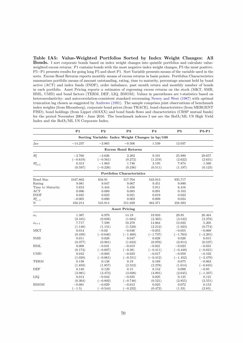
Table IA5: Value-Weighted Portfolios Sorted by Index Weight Changes: AllBonds. I sort corporate bonds based on index weight changes into quintile portfolios and calculate value-weighted excess returns. P1 contains bonds with the most negative index weight changes, P5 the most positive.P5−P1 presents results for going long P5 and short P1. Sort Variable presents means of the variable used in thesorts. Excess Bond Returns reports monthly means of excess returns in basis points. Portfolios Characteristicssummarizes portfolio means of amount outstanding, rating, time to maturity, percentage amount held by bondactive (ACT) and index funds (INDF), order imbalance, past month return and monthly number of bondsin each portfolio. Asset Pricing reports α estimates of regressing excess returns on the stock (MKT, SMB,HML, UMD) and bond factors (TERM, DEF, LIQ, BMOM). Values in parentheses are t-statistics based onheteroscedasticity- and autocorrelation-consistent standard errorsusing Newey and West (1987) with optimaltruncation lag chosen as suggested by Andrews (1991). The sample comprises joint observations of benchmarkindex weights (from Bloomberg), corporate bond prices (from TRACE), bond characteristics (from MERGENTFISD), bond holdings (from Lipper eMAXX) and bond funds flows and characteristics (CRSP mutual funds)for the period November 2004 - June 2016. The benchmark indexes I use are the BofA/ML US High YieldIndex and the BofA/ML US Corporate Index.

P1 P2 P3 P4 P5 P5-P1

Sorting Variable: Index Weight Changes in bp/100

∆w −14.237 −2.865 −0.506 1.539 12.037

Excess Bond Returns

Ret −3.766 −3.626 2.202 9.101 25.890 29.657(−0.619) (−0.561) (0.272) (1.219) (2.622) (2.631)

Ret+1 6.313 −1.863 1.746 3.195 7.874 1.560(0.597) (−0.226) (0.236) (0.511) (1.197) (0.123)

Portfolios Characteristics

Bond Size 1047.802 634.91 517.704 543.913 935.717Rating 9.081 9.047 9.067 9.451 9.890Time to Maturity 5.653 5.444 5.456 5.911 6.416ACT 0.096 0.089 0.085 0.091 0.103INDF 0.025 0.023 0.021 0.019 0.022Ret−1 −0.005 0.000 0.003 0.009 0.024N 456.214 545.814 551.029 482.371 358.393

Asset Pricing

αt 1.387 6.979 14.19 19.933 29.85 28.464(0.165) (0.828) (1.684) (2.365) (3.542) (3.378)

αt+1 7.717 7.599 10.278 14.864 12.922 5.205(1.148) (1.131) (1.529) (2.212) (1.923) (0.774)

MKT 0.014 −0.02 −0.046 −0.055 −0.055 −0.069(0.438) (−0.646) (−1.468) (−1.737) (−1.763) (−2.201)

SMB 0.011 0.028 0.047 0.028 0.026 0.015(0.377) (0.981) (1.632) (0.976) (0.914) (0.537)

HML 0.009 −0.031 −0.019 −0.021 −0.023 −0.031(0.174) (−0.607) (−0.38) (−0.411) (−0.448) (−0.621)

UMD 0.042 −0.003 −0.023 −0.017 −0.059 −0.102(1.028) (−0.061) (−0.551) (−0.412) (−1.452) (−2.479)

TERM 0.138 0.138 0.19 0.169 0.075 −0.063(1.859) (1.857) (2.552) (2.278) (1.014) (−0.845)

DEF 0.148 0.129 0.15 0.152 0.098 −0.05(3.981) (3.473) (4.038) (4.091) (2.645) (−1.337)

LIQ 0.014 −0.042 −0.035 0.025 0.135 0.121(0.304) (−0.892) (−0.748) (0.521) (2.855) (2.551)

BMOM −0.081 −0.029 −0.012 0.025 0.072 0.153(−1.5) (−0.544) (−0.232) (0.472) (1.33) (2.83)

70

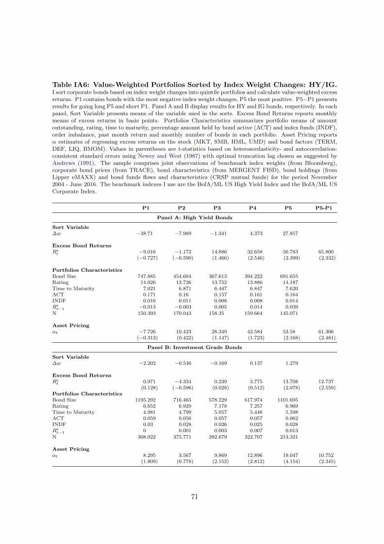
Table IA6: Value-Weighted Portfolios Sorted by Index Weight Changes: HY/IG.I sort corporate bonds based on index weight changes into quintile portfolios and calculate value-weighted excessreturns. P1 contains bonds with the most negative index weight changes, P5 the most positive. P5−P1 presentsresults for going long P5 and short P1. Panel A and B display results for HY and IG bonds, respectively. In eachpanel, Sort Variable presents means of the variable used in the sorts. Excess Bond Returns reports monthlymeans of excess returns in basis points. Portfolios Characteristics summarizes portfolio means of amountoutstanding, rating, time to maturity, percentage amount held by bond active (ACT) and index funds (INDF),order imbalance, past month return and monthly number of bonds in each portfolio. Asset Pricing reportsα estimates of regressing excess returns on the stock (MKT, SMB, HML, UMD) and bond factors (TERM,DEF, LIQ, BMOM). Values in parentheses are t-statistics based on heteroscedasticity- and autocorrelation-consistent standard errors using Newey and West (1987) with optimal truncation lag chosen as suggested byAndrews (1991). The sample comprises joint observations of benchmark index weights (from Bloomberg),corporate bond prices (from TRACE), bond characteristics (from MERGENT FISD), bond holdings (fromLipper eMAXX) and bond funds flows and characteristics (CRSP mutual funds) for the period November2004 - June 2016. The benchmark indexes I use are the BofA/ML US High Yield Index and the BofA/ML USCorporate Index.

P1 P2 P3 P4 P5 P5-P1

Panel A: High Yield Bonds

Sort Variable∆w −38.71 −7.989 −1.341 4.373 27.857

Excess Bond ReturnsRet −9.016 −1.172 14.886 32.658 56.783 65.800

(−0.727) (−0.590) (1.466) (2.546) (2.399) (2.332)

Portfolios CharacteristicsBond Size 747.885 454.684 367.613 394.222 691.655Rating 14.026 13.726 13.752 13.886 14.187Time to Maturity 7.021 6.871 6.447 6.847 7.620ACT 0.171 0.16 0.157 0.161 0.164INDF 0.016 0.011 0.008 0.008 0.014Ret−1 −0.013 −0.003 0.005 0.014 0.039N 150.393 170.043 158.35 159.664 145.071

Asset Pricingαt −7.726 10.423 28.349 42.584 53.58 61.306

(−0.313) (0.422) (1.147) (1.723) (2.168) (2.481)

Panel B: Investment Grade Bonds

Sort Variable∆w −2.202 −0.546 −0.169 0.137 1.279

Excess Bond ReturnsRet 0.971 −4.334 0.239 3.775 13.708 12.737

(0.128) (−0.596) (0.028) (0.512) (2.078) (2.559)Portfolios CharacteristicsBond Size 1195.292 716.465 578.229 617.974 1101.695Rating 6.652 6.929 7.178 7.257 6.969Time to Maturity 4.981 4.799 5.057 5.448 5.598ACT 0.059 0.056 0.057 0.057 0.062INDF 0.03 0.028 0.026 0.025 0.028Ret−1 0 0.001 0.003 0.007 0.013N 308.022 375.771 392.679 322.707 213.321

Asset Pricingαt 8.295 3.567 9.869 12.896 19.047 10.752

(1.809) (0.778) (2.152) (2.812) (4.154) (2.345)

71

Table IA7: Portfolios Sorted by Index Weight Changes: Including Assets Exiting-Entering the Index. I sort corporate bonds based on index weight changes into quintile portfolios andcalculate equally-weighted excess returns. P1 contains bonds with the most negative index weight changes,P5 the most positive. P5−P1 presents results for going long P5 and short P1. Panel A, B and C displayresults for all bonds, HY bonds and IG bonds, respectively. In each panel, Sort Variable presents means ofthe variable used in the sorts. Excess Bond Returns reports monthly means of excess returns in basis points.Asset Pricing reports α estimates of regressing excess returns on the stock (MKT, SMB, HML, UMD) andbond factors (TERM, DEF, LIQ, BMOM). Values in parentheses are t-statistics based on heteroscedasticity-and autocorrelation-consistent standard errors using Newey and West (1987) with optimal truncation lagchosen as suggested by Andrews (1991). The sample comprises joint observations of benchmark index weights(from Bloomberg), corporate bond prices (from TRACE), bond characteristics (from MERGENT FISD), bondholdings (from Lipper eMAXX) and bond funds flows and characteristics (CRSP mutual funds) for the periodNovember 2004 - June 2016. The benchmark indexes I use are the BofA/ML US High Yield Index and theBofA/ML US Corporate Index.

P1 P2 P3 P4 P5 P5-P1

Panel A: All Bonds

Sort Variable∆w −19.33 −2.877 −0.506 1.539 28.827

Excess Bond ReturnsRet −8.221 −4.427 0.023 11.565 31.036 39.257

(−1.109) (−0.639) (0.003) (1.507) (2.983) (2.888)Ret+1 −1.273 −1.357 1.835 4.528 7.518 8.791

(−0.16) (−0.161) (0.212) (0.68) (1.158) (0.883)Asset Pricingαt 0.151 7.755 13.823 23.674 37.559 37.408

(0.017) (0.873) (1.556) (2.665) (4.229) (4.212)αt+1 4.837 8.93 12.793 17.548 16.095 11.258

(0.763) (1.409) (2.018) (2.768) (2.539) (1.776)

Panel B: High Yield Bonds

Sort Variable∆w −49.243 −7.989 −1.343 4.372 65.579

Excess Bond ReturnsRet −20.528 −7.084 3.462 29.077 64.629 85.157

(−1.522) (−1.063) (0.38) (2.641) (3.098) (2.771)Ret+1 −11.615 −1.192 6.337 11.809 18.216 29.831

(−1.316) (−0.159) (0.708) (1.289) (1.653) (1.75)Asset Pricingαt −15.579 5.571 19.002 42.407 68.094 83.673

(−0.728) (0.26) (0.888) (1.982) (3.182) (3.91)αt+1 1.821 14.865 18.854 21.5 16.494 14.673

(0.13) (1.06) (1.345) (1.533) (1.176) (1.046)

Panel C: Investment Grade Bonds

Sort Variable∆w −5.235 −0.566 −0.169 0.137 2.787

Excess Bond ReturnsRet −0.366 −3.479 −0.456 4.896 14.867 15.232

(−0.045) (−0.474) (−0.059) (0.699) (2.161) (2.734)Ret+1 2.94 −0.536 −0.257 1.389 2.012 −0.928

(0.294) (−0.057) (−0.031) (0.225) (0.41) (−0.097)Asset Pricingαt 9.73 6.595 10.636 14.656 21.983 12.253

(2.31) (1.566) (2.525) (3.479) (5.219) (2.909)αt+1 8.431 6.918 8.574 14.258 12.209 3.778

(1.384) (1.136) (1.408) (2.341) (2.005) (0.62)

72

Table IA8: Regression-Based Tests - Time Variation. I present results of regressionsexploring the link between corporate bond monthly excess returns and benchmark index weight changes. Reit(in bps) is the dependent variable in all models. The control variables comprise a set of bond characteristics,lagged returns and fund flows. I include one dummy for each of the quintile portfolios sorted on index weightchanges, except for P1, which is the reference dummy. I furthermore include a dummy for the time periodsJanuary 2008 - December 2011 and January 2012 - June 2016. The sample comprises joint observations ofbenchmark index weights (from Bloomberg), corporate bond prices (from TRACE), bond characteristics (fromMERGENT FISD), bond holdings (from Lipper eMAXX) and bond funds flows and characteristics (CRSPmutual funds) for the period November 2004 - June 2016. The benchmark indexes I use are the BofA/ML USHigh Yield Index and the BofA/ML US Corporate Index. All t-statistics (given in parentheses) are based onstandard errors clustered at the issuer level.

All Bonds IG HY

P2-P1 −2.257 −5.209∗∗∗ 4.494(−1.575) (−4.534) (1.058)

P3-P1 −0.676 −6.053∗∗∗ 10.580∗∗

(−0.430) (−4.708) (2.199)

P4-P1 9.096∗∗∗ −1.501 31.154∗∗∗

(5.340) (−1.108) (6.533)

P5-P1 12.673∗∗∗ 2.096 34.144∗∗∗

(4.142) (1.234) (4.318)

12012−2016 −5.139∗∗∗ −5.359∗∗∗ 8.271∗

(−3.401) (−4.018) (1.686)

12008−2011 3.041∗ 2.051 14.840∗∗

(1.666) (1.357) (2.513)

(P5-P1) ×12012−2016 11.244∗∗∗ 13.050∗∗∗ 11.115(3.219) (5.975) (1.193)

(P5-P1) ×12008−2011 19.815∗∗∗ 11.884∗∗ 33.703∗∗∗

(3.698) (2.466) (2.766)

Observations 274,935 188,204 86,731Adjusted R2 0.015 0.015 0.020Intercept Yes Yes YesIssuer FE Yes Yes YesClustered SE Yes Yes Yes

73