The impact of asset price bubbles on liquidity risk ...
31
152 Int. J. Bonds and Derivatives, Vol. 2, No. 2, 2016 Copyright © 2016 Inderscience Enterprises Ltd. The impact of asset price bubbles on liquidity risk measures from a financial institutions perspective Michael Jacobs Jr. Accenture Consulting, Finance and Risk Services Advisory/Models, Methodologies & Analytics, 1345 Avenue of the Americas, New York, N.Y., 10105, USA Email: [email protected] Abstract: This study presents an analysis of the impact of asset price bubbles on a liquidity risk measure, the liquidity risk option premium (‘LROP’). We present a styled model of asset price bubbles in continuous time, and perform a simulation experiment of a stochastic differential equation (‘SDE’) system for the asset value through a constant elasticity of variance (‘CEV’) process. Comparing bubble to non-bubble economies, it is shown that asset price bubbles may cause an firm’s traditional risk measures, such as value-at-risk (‘VaR’) to decline, due to an increase in the right skewness of the value distribution, which results in the LROP to decline and therefore an underpricing of liquidity risk. Keywords: financial crisis; liquidity risk; model risk; asset price bubbles; value-at-risk; stochastic differential equation; SDE; constant elasticity of variance; CEV. Reference to this paper should be made as follows: Jacobs Jr., M. (2016) ‘The impact of asset price bubbles on liquidity risk measures from a financial institutions perspective’, Int. J. Bonds and Derivatives, Vol. 2, No. 2, pp.152–182. Biographical notes: Michael Jacobs Jr., PhD, CFA, is a Principal Director in the Risk Analytics practice of Accenture. He specialises in risk model development and validation across a range of risk and product types. He has 25 years of experience in financial risk modelling and analytics, having worked five year for Deloitte and PwC as a Director in the risk modelling and analytics practice, with a focus on regulatory solutions; seven years as a Senior Economist and Lead Modelling Expert at the OCC, focusing on ERM and Model Risk; and eight years in banking as a Senior Vice-President at JPMC and SMBC, developing wholesale credit risk and economic capital models. 1 Introduction and motivations The financial crisis of the last decade has been the impetus behind a movement to better understand the relative merits of various risk measures, classic examples being value-at-risk (‘VaR’) and related quantities (Jorion, 2006; Inanoglu and Jacobs, 2009). The importance of an augmented comprehension of these measures is accentuated in the
Transcript of The impact of asset price bubbles on liquidity risk ...

152 Int. J. Bonds and Derivatives, Vol. 2, No. 2, 2016
Copyright © 2016 Inderscience Enterprises Ltd.
The impact of asset price bubbles on liquidity risk measures from a financial institutions perspective
Michael Jacobs Jr. Accenture Consulting, Finance and Risk Services Advisory/Models, Methodologies & Analytics, 1345 Avenue of the Americas, New York, N.Y., 10105, USA Email: [email protected]
Abstract: This study presents an analysis of the impact of asset price bubbles on a liquidity risk measure, the liquidity risk option premium (‘LROP’). We present a styled model of asset price bubbles in continuous time, and perform a simulation experiment of a stochastic differential equation (‘SDE’) system for the asset value through a constant elasticity of variance (‘CEV’) process. Comparing bubble to non-bubble economies, it is shown that asset price bubbles may cause an firm’s traditional risk measures, such as value-at-risk (‘VaR’) to decline, due to an increase in the right skewness of the value distribution, which results in the LROP to decline and therefore an underpricing of liquidity risk.
Keywords: financial crisis; liquidity risk; model risk; asset price bubbles; value-at-risk; stochastic differential equation; SDE; constant elasticity of variance; CEV.
Reference to this paper should be made as follows: Jacobs Jr., M. (2016) ‘The impact of asset price bubbles on liquidity risk measures from a financial institutions perspective’, Int. J. Bonds and Derivatives, Vol. 2, No. 2, pp.152–182.
Biographical notes: Michael Jacobs Jr., PhD, CFA, is a Principal Director in the Risk Analytics practice of Accenture. He specialises in risk model development and validation across a range of risk and product types. He has 25 years of experience in financial risk modelling and analytics, having worked five year for Deloitte and PwC as a Director in the risk modelling and analytics practice, with a focus on regulatory solutions; seven years as a Senior Economist and Lead Modelling Expert at the OCC, focusing on ERM and Model Risk; and eight years in banking as a Senior Vice-President at JPMC and SMBC, developing wholesale credit risk and economic capital models.
1 Introduction and motivations
The financial crisis of the last decade has been the impetus behind a movement to better understand the relative merits of various risk measures, classic examples being value-at-risk (‘VaR’) and related quantities (Jorion, 2006; Inanoglu and Jacobs, 2009). The importance of an augmented comprehension of these measures is accentuated in the

The impact of asset price bubbles on liquidity risk measures 153
realm of liquidity risk, as the price bubble in the housing market and the ensuing credit crunch was directly related to a deficit in liquidity for market participants, which in turn was undoubtedly one of the major catalysts for the financial crisis. We have subsequently learned from this that the risk models of that era failed in not incorporating the phenomenon of asset price bubbles, which in turn added to the severity of the downturn for investors and risk managers who mis-measured their potential adverse exposure to liquidity risk. This manifestation of model risk (The U.S. Board of Governors of the Federal Reserve System, 2011), wherein a modelling framework lacks a key element of an economic reality and therefore fails, was due to some extent to a lack of basic understanding. This failure of the modelling paradigm in liquidity risk spans gaps in the measurement, characterisation and economics of asset price bubbles.
Since asset price bubbles are inevitably bound to burst, causing significant value loss to shareholders, more economic capital should be held for these bubble-bursting scenarios. Unfortunately, the severity of these bubble-bursting scenarios is not adequately captured by the standard risk measures, whose computation is based on the standard moments and quantiles of a firm’s value distribution over time horizons such as a year, over which bubble bursting is unlikely. Therefore, in view of analysing the impact of asset price bubbles on liquidity risk measures and economic capital determination of a firm, we construct various hypothetical economies, having and also not having asset price bubbles. We present a model of asset price bubbles in continuous time, and perform a simulation experiment of a stochastic differential equation (‘SDE’) for asset value through a constant elasticity of variance (‘CEV’) process1. The results of our experiment demonstrate that the existence of an asset price bubble, which occurs for certain parameter settings in the CEV model, results in the firm’s asset value distribution having a greater right skewness. This augmented right skewness in of the firm’s asset value distribution due to bubble expansion results in the firm’s VaR measures to decline, an understatement in the equity risk of the firm. We furthermore propose a liquidity risk measure by modelling the liquidity risk premium as the price of a down and out call option on the equity price, the liquidity risk option premium (‘LROP’), and show that it declines as we move from a non-bubble to a bubble economy. In turn, as the LROP is modelled as a down-and-out option on the equity value, based on these measures alone their declining values imply that in the presence of asset price bubbles, the result is a lower estimate for required liquidity risk on the part of investors and risk managers. We conclude that such bubble phenomena must be taken into consideration for the proper determination of economic capital for risk management and measurement purposes.
‘Liquidity’ or the related risk is not always well-defined, but herein we try:
• Definition 1: Liquidity represents the capacity to fulfil all payment obligations as and when they come due, to the full extent and in the proper currency, on a purely cash basis.
• Definition 2: Liquidity risk is the danger and accompanying potential undesirable effects of not being able to accomplish the above.
This basic definition says that liquidity is neither an amount nor ratio, but the degree to which a bank can fulfil its obligations, in this sense a qualitative element in the financial strength of a firm. A characteristic of liquidity is that is must be available all the time, not just on average; therefore, failure to perform, while a low probability event, implies potentially severe or even fatal consequences. While liquidity events occur more

154 M. Jacobs Jr.
frequently and with less severity than extreme stress events, they are sufficiently dangerous to disrupt business and alter the strategic direction of a firm.
Inanoglu and Jacobs (2009) develops models for risk aggregation and sensitivity analysis, with an application to bank economic capital. The authors proxy for risk types from quarterly financial bank data submitted to the regulators: credit risk by gross charge-offs, operational risk by other non-interest expense, market risk by the deviation in four-quarter average trading revenues, interest rate risk by the deviation in the four-quarter average interest rate gap (i.e., rate on deposits minus loans), and liquidity risk by the deviation in four-quarter average liquidity gap (i.e., loans minus deposits). As shown in Table 1, generally this measure of liquidity risk exhibits positive and sometimes substantial correlation with other risk types. Table 1 Correlations amongst risk types – top 200 largest banks and five largest banks risk
proxies
Risk pair Aggregate Banks
JP Morgan Chase
Bank of America Citigroup Wells
Fargo PNC
Credit and liquidity risk
53.43% 19.07% 47.87% 31.47% 2.30% 20.85%
Interest rate and liquidity risk
15.33% 7.37% –8.55% 11.76% –4.85% –10.22%
Market and liquidity risk
11.27% 1.56% –18.23% 6.29% –0.94% –3.21%
Operational and liquidity risk
18.97% 19.96% 9.17% 12.38% 9.14% 12.86%
Figure 1 Liquidity measure leading up to the financial crisis – average liquidity ratios for the top 50 banks as of 4Q09 (see online version for colours)
0
0.02
0.04
0.06
0.08
0.1
0.12
1984
0331
1984
0930
1985
0331
1985
0930
1986
0331
1986
0930
1987
0331
1987
0930
1988
0331
1988
0930
1989
0331
1989
0930
1990
0331
1990
0930
1991
0331
1991
0930
1992
0331
1992
0930
1993
0331
1993
0930
1994
0331
1994
0930
1995
0331
1995
0930
1996
0331
1996
0930
1997
0331
1997
0930
1998
0331
1998
0930
1999
0331
1999
0930
2000
0331
2000
0930
2001
0331
2001
0930
2002
0331
2002
0930
2003
0331
2003
0930
2004
0331
2004
0930
2005
0331
2005
0930
2006
0331
2006
0930
2007
0331
2007
0930
2008
0331
2008
0930
2009
0331
2009
0930
The impact of asset price bubbles on liquidity risk measures 155
Figure 1 is reproduced from Inanoglu et al. (2015), who study the efficiency of the banking system in the period leading up to the financial crisis, showing that as banks grew larger and took on more risk they also became less efficient. The authors develop a liquidity measure as the ratio of liquid assets to total value of banking book. Note the secular decline in liquidity during 20 years going into recent crisis (except a 1990 spike), more recently a rapid and massive increase from the depth to the end of the crisis.
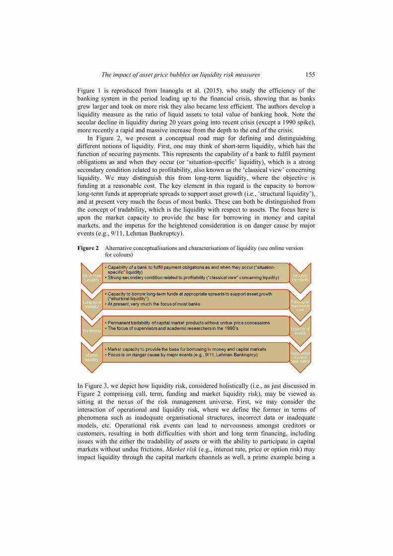
In Figure 2, we present a conceptual road map for defining and distinguishing different notions of liquidity. First, one may think of short-term liquidity, which has the function of securing payments. This represents the capability of a bank to fulfil payment obligations as and when they occur (or ‘situation-specific’ liquidity), which is a strong secondary condition related to profitability, also known as the ‘classical view’ concerning liquidity. We may distinguish this from long-term liquidity, where the objective is funding at a reasonable cost. The key element in this regard is the capacity to borrow long-term funds at appropriate spreads to support asset growth (i.e., ‘structural liquidity’), and at present very much the focus of most banks. These can both be distinguished from the concept of tradability, which is the liquidity with respect to assets. The focus here is upon the market capacity to provide the base for borrowing in money and capital markets, and the impetus for the heightened consideration is on danger cause by major events (e.g., 9/11, Lehman Bankruptcy).
Figure 2 Alternative conceptualisations and characterisations of liquidity (see online version for colours)
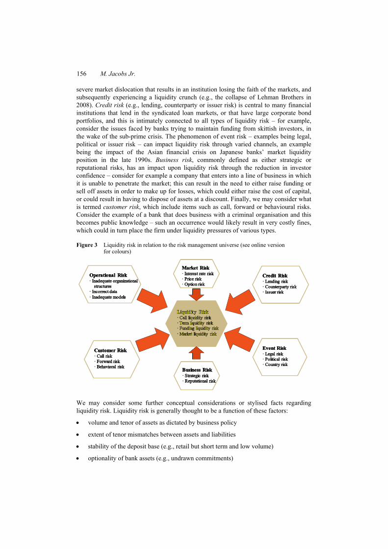
In Figure 3, we depict how liquidity risk, considered holistically (i.e., as just discussed in Figure 2 comprising call, term, funding and market liquidity risk), may be viewed as sitting at the nexus of the risk management universe. First, we may consider the interaction of operational and liquidity risk, where we define the former in terms of phenomena such as inadequate organisational structures, incorrect data or inadequate models, etc. Operational risk events can lead to nervousness amongst creditors or customers, resulting in both difficulties with short and long term financing, including issues with the either the tradability of assets or with the ability to participate in capital markets without undue frictions. Market risk (e.g., interest rate, price or option risk) may impact liquidity through the capital markets channels as well, a prime example being a
156 M. Jacobs Jr.
severe market dislocation that results in an institution losing the faith of the markets, and subsequently experiencing a liquidity crunch (e.g., the collapse of Lehman Brothers in 2008). Credit risk (e.g., lending, counterparty or issuer risk) is central to many financial institutions that lend in the syndicated loan markets, or that have large corporate bond portfolios, and this is intimately connected to all types of liquidity risk – for example, consider the issues faced by banks trying to maintain funding from skittish investors, in the wake of the sub-prime crisis. The phenomenon of event risk – examples being legal, political or issuer risk – can impact liquidity risk through varied channels, an example being the impact of the Asian financial crisis on Japanese banks’ market liquidity position in the late 1990s. Business risk, commonly defined as either strategic or reputational risks, has an impact upon liquidity risk through the reduction in investor confidence – consider for example a company that enters into a line of business in which it is unable to penetrate the market; this can result in the need to either raise funding or sell off assets in order to make up for losses, which could either raise the cost of capital, or could result in having to dispose of assets at a discount. Finally, we may consider what is termed customer risk, which include items such as call, forward or behavioural risks. Consider the example of a bank that does business with a criminal organisation and this becomes public knowledge – such an occurrence would likely result in very costly fines, which could in turn place the firm under liquidity pressures of various types.
Figure 3 Liquidity risk in relation to the risk management universe (see online version for colours)
We may consider some further conceptual considerations or stylised facts regarding liquidity risk. Liquidity risk is generally thought to be a function of these factors:
• volume and tenor of assets as dictated by business policy
• extent of tenor mismatches between assets and liabilities
• stability of the deposit base (e.g., retail but short term and low volume)
• optionality of bank assets (e.g., undrawn commitments)

The impact of asset price bubbles on liquidity risk measures 157
• persistence of a liquidity gap with the implication that the bank will have to get funding
• terms of later financing not known in advance
• even marketable assets having different liquidity characteristics over time
• willingness of the market to fund dependent upon the future state of the bank
• dependence of the bank’s financial state and perception of such in the market upon inter-related data (e.g., risk profile, solvency, profitability and trend)
• bank’s forecast of its own state and the market perception of this are both risky and uncertain.
We may also consider alternative ways to look at liquidity risk. First, there is the level of aggregation, which may include several dimensions such as amount, currency and time horizon. It is advisable to maintain as detailed information as possible, even if not required by controllers or supervisors. Second, there is the concept of natural (i.e., legal maturities) vs. artificial (i.e., shiftability and marketability – the ‘business view’) liquidity, and the importance of meeting customers’ needs and keeping the franchise intact (not just surviving as a legal entity). There are also optionalities, which apply not only to traded or OTC options, but any bank commitment that puts the bank in a position of an option seller exposed to unpredictable cash requirements. Finally, there is the impact of business policy on liquidity, namely the need for a dynamic perspective, and the important distinction between accounting and actual cash flows.
Another aspect to consider is the interconnection between liquidity risk and other risks. Solvency is the condition of sufficient capital to cover loss, a pre-condition but not sufficient for liquidity, as perceived solvency can impact liquidity through the actions of investors or customer. Then there is the distinction between liquidity and interest rate risk, as prima facie it seems that they can be treated similarly with respect to gap analysis, but for a typical bank’s exposure it is unlikely that they form a predictable relationship. As an example, consider prepayment: here we have excess liquidity but reinvestment rate risk; also, a case where a CP line is triggered, which may have hedged rates with forward rate agreements, but the actual exchange of cash gives rise to liquidity risk.. Another important distinction is liquidity as opposed to market liquidity risk, as the ability to transform marketable assets into cash depends upon the breadth and depth of markets, which in turn depends on the quality of the issuer, market conditions and asset characteristics. Finally, we may consider the two alternative ways to close the liquidity gap: international financial institutions’ ‘asset driven’ vs. savings banks ‘liability driven’ strategies, but however note that the latter depends on behaviour of lenders, and on name of institution and market.
The quantification of liquidity risk encompasses four key aspects:
• behaviour of the balance sheet structure under various circumstances
• basic conditions required when applying a dynamic business perspective
• forecasting the most likely liquidity gaps
• linking these findings to liquidity policy.
158 M. Jacobs Jr.
Two basic occurrences lead to increased liquidity risk:
• assets marketable assets loose quality or segment for which is congested
• liabilities funding potential declines.
Key components of a quantitative liquidity risk framework include:
• dynamism: planned and future developments need to be accounted for
• distinctiveness between normal and stressed environments
• accounting for that circumstances can vary in quality
• accounting for the heterogeneity of impact upon particular banks
• forward looking orientation.
An outline for this paper is as follows. Section 2 presents a review of the literature on risk measurement and also on liquidity risk. Section 3 presents our model incorporating the effect of asset price bubbles into the measurement of liquidity risk. Section 4 describes the results of our simulation experiment while Section 5 summarises the implications of our analysis for liquidity risk management and directions for future research.
2 Review of the literature
Modern risk modelling (e.g., Merton, 1974 for the case of credit risk) increasingly relies on advanced mathematical, statistical and numerical techniques to measure and manage risk in credit portfolios. This gives rise to model risk (The U.S. Board of Governors of the Federal Reserve System, 2011), defined as the potential that a model used to assess financial risks does not accurately capture those risks, and the possibility of understating inherent dangers stemming from very rare yet plausible occurrences perhaps not in reference datasets or historical patterns of data2, a key example of this being the inability of the risk modelling paradigm to accommodate the phenomenon of asset price bubbles.
The relative merits of various risk measures, classic examples being VaR and related quantities, have been discussed extensively by prior research (Jorion, 1997, 2006). Risk management as a discipline in its own right, distinct from either general finance or financial institutions, is a relatively recent phenomenon. A general result of mathematical statistics due to Sklar (1956), allowing the combination of arbitrary marginal risk distributions into a joint distribution while preserving a non-normal correlation structure, readily found an application in finance. Among the early academics to introduce this methodology is Embrechts et al. (1999, 2002, 2003). This was applied to credit risk management and credit derivatives by Li (2000). The notion of copulas as a generalisation of dependence according to linear correlations is used as a motivation for applying the technique to understanding tail events in Frey and McNeil (2001). This treatment of tail dependence contrasts to Poon et al. (2004), who instead use a data intensive multivariate extension of extreme value theory, which requires observations of joint tail events.
Since the 2007 crisis, the mathematical finance literature has made significant advances in the modelling and testing of asset price bubbles (Hong et al., 2006; Jarrow and Protter, 2010; Protter, 2011). Inanoglu and Jacobs (2009) contribute to the modelling

The impact of asset price bubbles on liquidity risk measures 159
effort by providing tools and insights to practitioners and regulators, utilising data from major banking institutions’ loss experience, exploring the impact of business mix and inter-risk correlations on total risk, and comparing alternative established frameworks for risk aggregation on the same datasets across banks. Jarrow and Silva (2014) apply these new insights to determine the impact, if any, that asset price bubbles have on the common risk measures used in practice for the determination of equity capital, which we extend to the realm of credit risk. Jacobs (2015) extends the latter framework to credit risk measurement in a Merton (1974) structural model framework, wherein the author demonstrates that in the presence of asset price bubbles, standard credit risk quantile measures (e.g., credit VaR) are understated.
There is rather limited literature on the measurement, modelling and management of liquidity risk that are relevant to this current research, but we summarise a few key studies herein. Knies (1876) stresses the necessity for a cash buffer to bridge negative payment gaps between inflows and outflows where timing is uncertain. Stutzel (1959) provides further discussions focusing primarily on basic considerations between liquidity and solvency. A new focus emerged starting in mid-1990s was on specific issue of liquidity risk management, mainly dealing with policy (Matz, 2002; Baretsky et al., 2008). The Basel Committee on Banking Supervision (BCBS, 2006) provide supervisory expectations and best practices for managing liquidity risk in financial institutions. Fielder (2007), Hiedorn and Schamlz (2008) and Reitz (2008) provide quantitative frameworks for measuring and managing liquidity risk. Duttweiler (2008) provides a holistic view of liquidity risk including quantitative methods such as liquidity-at-risk (‘LaR’).
3 An option theoretic model for asset price bubbles and the pricing of liquidity risk
We model the evolution of asset prices, incorporating the phenomenon of price bubbles, using the approach of Jarrow et al. (2007) and Jarrow and Silva (2014). The setting is a continuous trading economy, without loss of generality having a finite horizon [0, τ], with randomness described by the filtered probability space (Ω, ℑ, F, P) where we define: the state space Ω, the σ-algebra ℑ, the information partition F = {ℑt}t∈[0,τ], and the physical probability measure P (or actuarial, as contrasted to a risk-neutral probability measure, commonly denoted by the symbol Q). We assume, again without loss of generality and for the purpose on focusing on the application to loss, a single asset value process {Vt}t∈[0,τ] that is adapted to the filtration F. Note that this could also represent a share of stock owned by a representative equity investor, which is a claim on the single productive entity or firm in this economy. In our options model of the liquidity risk premium, this is a postulated reference process (e.g., an equity index) that shadows the perceived value of the illiquid asset, and we are concerned that long-term investors may withdraw funds if it falls below a threshold. In the general setting, Vt follows an Ito diffusion process (Øksendal, 2003) having the following SDE representation:
( ) ( ), , ,t t tdV μ V t dt σ V t dW= + (3.1)

160 M. Jacobs Jr.
where μ(Vt, t) is the instantaneous drift process, σ(Vt, t) is the instantaneous diffusion process, Wt ~ N(0, t) is a standard Weiner process (or a Brownian motion process) on the filtered probability space (Ω, ℑ, F, P), and dWt are its infinitesimal increments. In order to complete this economy, we assume that there exists a traded money market account process, Mt which grows according to a risk-free rate process rt, also adapted to the filtration F of the aforementioned probability space:
{ }0
expt
t ss
M r ds=
= ∫ (3.2)
Without loss of generality we assume that the asset Vt has no cash-flows, which could have been incorporated into the model by assuming a dividend process and studying the dividend-reinvested stock price process (Back, 2010), but to maintain simplicity of notation we do not do not do so.
We model an economy potentially having an price bubbles through the assumption that the risky asset’s prices follows a CEV process, as in Jarrow et al. (2014), which is the following restricted version of the Ito diffusion process in (3.1):
θt t ttdV μV dt σV dW= + (3.3)
where μ is the drift, σ is the volatility and the CEV parameter θ governs the state of the risky asset price process exhibiting a price bubble or not. An asset price bubble is defined as the situation where the market price for an asset exceeds its fundamental value (Jarrow et al., 2007, 2010a, 2010b), the latter being defined conventionally as the price an investor would pay to hold the asset perpetually without rebalancing. This fundamental value is determined through imposing some additional structure on the economy, requiring at minimum two additional assumptions. First, we need to assume the absence of any arbitrage opportunities (Delbaen and Schachermayer, 1998), which guarantees the existence of a risk-neutral probability Q measure equivalent to P, such that the asset value process Vt normalised by the money market account Mt is a local Martingale process:
( )*
*,τ t τtQt t
t t
VVE V t tM M
−
′
⎡ ⎤⎡ ⎤′⎢ ⎥ℑ = = ∀ <⎢ ⎥
⎢ ⎥⎣ ⎦⎣ ⎦ (3.4)
where **( , )
τt t τV V −≡ is the stopped process of Vt and τ*: Ω → [0, +∞] is a sequence of
stopping times that satisfy certain technical condition.3 The mechanism in (3.4) involving the risk-neutral probability measure affords us a means of computing present values where we shift the mass of the probability distribution (magnitude of the cash-flows) such that we can recover the same prices as under actuarial measure with the original cash-flows – but note that Q is arbitrary. In order to pin down this risk-neutral distribution, we assume from this point on a complete market, which means that that enough derivatives on the risky assets trade in order to replicate its cash flows in a suitably constructed arbitrage portfolio. The first condition is satisfied because the CEV process given in expression (3.3) admits an equivalent local martingale measure, so by construction it satisfies the absence of arbitrage opportunities4. Under this incremental structure that we impose upon the economy, an asset’s fundamental value FVt given the time t information set ℑt, is defined as the asset’s discounted future payoff from liquidation at time at horizon τ > t:
The impact of asset price bubbles on liquidity risk measures 161
[ ]| τQt t t t t
τ
VFV V E MM⎡ ⎤
ℑ = ℑ⎢ ⎥⎣ ⎦
(3.5)
It follows that we may define the asset’s price bubble B [ ]Vt • as the difference between
the market price Vt and its fundamental value FVt:
[ ] [ ]BVt t t t t tt V V FV Vℑ ≡ − ℑ (3.6)
Since as a conditional expectation, the fundamental value normalised by the value of the money market account is a martingale under Q, a bubble exists if and only if the asset’s normalised price is a strict local martingale and not a martingale under Q. In the case of the CEV process, it can be shown (Jarrow et al., 2011) that the asset’s normalised price
( )t
t
VM
is a martingale under Q when θ ≤ 1 in (3.3) (i.e., no asset price bubble), and a
strict-local martingale under Q where θ > 1 in that equation (i.e., an asset price bubble). Note that the boundary case of θ = 1 yields the geometric Brownian motion underlying the Black-Scholes-Merton (‘BSM’) option pricing model (Merton, 1974), which is called the BSM economy, and can be shown to exhibit no price bubble (Delbaen and Schachermayer, 1995). In such case we have:
( )t t t tdV μ r V dt σV dW= − + (3.7)
It follows that the reference process is log-normally distributed 0
ln( ) ~ ([tV N μ rV
− −
2 21 ] , ).2σ t σ t We will illustrate how to model the LROP in the BSM framework following
Golts and Kritzman (2010), in which we can obtain a closed-form solution. Let the
absolute barrier be denoted as B ≤ V0 and the relative barrier be denoted as 0
,BcV
= the
latter being the complement of the percent decline that triggers the option to be in the money. Therefore we model this contingent claim as a first passage option having the following payoff at maturity τ and strike price K:
0
[0, ] 0
0min t rtt τ
cV BV
cV e B K∈
> = ⇒⎧= ⎨≤ ⇒ =⎩
(3.8)
In the case of the BSM model we get the following closed form solution:
( ) ( ) ( )( )0 2 0 1Π , , , , rτ rτFP V B σ r τ e KN d V e N d−= − + − (3.9)
where 2
01 2
1 ln( ) ( )2
V σd τ r d σ τKσ ρ
= + + = + and the price of the option per $1
notional is given by:
( )0,1
0
Π , , , ,Π (1, , , , ) 1FP
FPV B σ r τ
B σ r τV
= ≤ (3.10)
162 M. Jacobs Jr.
Assume a T period investment horizon with m equally spaced liquidity intervals of length τ = Ti – Ti–1 for i = 1,..,m, which implies that 0 = T0 ≤ T1 ≤ … ≤ Tm = T = mτ. We model an illiquid instrument as a long position in the liquid reference process with price V* < V0, and a short position in an m period liquidity option of value V0 – V*, a collection of m – 1 first passage options (also known collectively as a ‘cliquet option’). If we define a cash call event as a log return of –100% over the entire period T, then we can solve for the barrier as a proportion of initial value as:
0expB τc
V T τ⎛ ⎞
= = −⎜ ⎟−⎝ ⎠
(3.11)
This shows the barrier to be higher (lower) for investors with shorter (longer) liquidity intervals τ, and to be increasing in maturity T. Denote C(t) as the cash in the replicating portfolio at period t; then for Ti – T (at T the asset matures and no payoff) the payoff on the ith option is:
[ ]
( )( ) ( ) ( )11
1
, 1 1
0min
i ii i
it r T Tt T T i i
cC TV
cC T e C T−−
−
−∈ − −
⎧> ⇒= ⎨
≤ ⇒⎩ (3.12)
The normalised price of the option in the first interval is just as before:
( ) ( ),1 0 0 0Π , , , , Π 1, , , , ΠFP FPV B σ r τ B σ r τ V V= (3.13)
The expected cash position at the end of the initial period is:
( ) ( )1 1 1
10 1 0
[0, ]Pr min (1 Π)rT rT rT
e tt T
E C V e Be V B S e∈
= − ≤ = − (3.14)
Continuing on this reasoning, and imposing that under risk-neutral measure 10 ( )TE V = 1( )
0 0 ,μ r TV e V− = as μ = r, we get for small Π the approximation:
( ) ( )1
1, 1 0 0 0
0
Π , , , , Π (1 Π) 1 (1 Π) ( 1)Πm
k mFP m
k
V B σ r τ V V m−
−−
=
= − = − − ≈ −∑ (3.15)
If the number of liquidity intervals is 1,Tτ= then the barrier is
00,Bc
V= = the value of
the liquidity option is zero and there is no price difference between the liquid and illiquid assets. Conversely, if the investor needs immediate liquidity τ = 0 (i.e., an infinite number
of liquidity intervals), then the barrier is 0
1,BcV
= = and the price of the liquidity option
is 100% of the notional amount Π(•) = V0. We now develop various risk measures with respect to the reference process, which will help us gauge the inaccuracy of standard approaches as we move from a normal to a bubble economy. First, we define the expected value of the reference process EVτ as the expectation of this random variable under actuarial probability measure:
[ ]Pt τ tEV E V= ℑ (3.16)
The impact of asset price bubbles on liquidity risk measures 163
We may estimate this quantity as EVτ through numerical integration over np simulations, which is simply the sample mean, and is a consistent and unbiased estimator of this sample moment:
1
1 pNi
τ τp i
EV VN =
= ∑ (3.17)
Similarly, we may obtain estimators of the population standard deviation Vτσ and of the
population normalised skewness Vτς of this distribution, defined as:
( )2V Pτ τ τ tσ E V EV⎡ ⎤= − ℑ⎣ ⎦ (3.18)
( )
( )
3
23
Pτ τ tV
τECLτ
E V EVς
σ
⎡ ⎤− ℑ⎣ ⎦= (3.19)
by their sample analogues ˆVτσ and ˆ :V
τς
2
1 1
1 1ˆ1
p pN NV i iτ τ τ
p pi i
σ V VN N= =
⎡ ⎤= −⎢ ⎥
− ⎢ ⎥⎣ ⎦∑ ∑ (3.20)
[ ]
( )
3
12
3
1
ˆˆ
pNiτ τ
p iVτ
Vτ
V EVN
ςσ
=
−
=∑
(3.21)
These statistics are estimates of the reference process distribution’s moments under the physical probability measure P, characterising the changes in the value of the index that includes both positive and negative mark-to-market values. In a risk management application, we are actually only interested in losses, to which end we seek to understand the left tail of the value distribution, and compute various low quantile risk measures, such as the VaR or conditional value-at-risk (‘CVaR’). Apart from asset price bubbles, even though its limitations re-widely known (Alexander, 2001; Jorion, 1997), such measures are widely used in the industry5. An estimator for the VaR at a given confidence level c is given by:
( )( ) Quantile pτ i k N cVaR c ≤ ≤= (3.22)
where
( )1
1Quantile ( ) supp
kp τ
N
i k N c V xx p k
c I cN≤ ≤ ≤
=
⎧ ⎫⎡ ⎤⎪ ⎪= ≤⎢ ⎥⎨ ⎬
⎢ ⎥⎪ ⎪⎣ ⎦⎩ ⎭∑ (3.23)
where kτV xI ≤ is an indicator function that takes the value 1 if kτV x≤ and 0 otherwise. We
may also define a conditional CVaR measure as the expected value conditional on value being less than or equal to VaR at confidence level c:

164 M. Jacobs Jr.
( )1
( )1
( )
p
kτ
p
kτ
Nkτ V VaR c
kN
V VaR ck
V ICVaR c
I
≤=
≤=
=∑
∑ (3.24)
4 A simulation experiment
We demonstrate the impact of asset price bubbles on a firm’s risk measures, as defined in the previous section (i.e., VaR and CVaR), as well as on the measure of liquidity risk the LROP, through a stochastic simulation experiment. Simulation is needed to determine the probability distribution of the asset value (or reference process), and ultimately the LROP, because an analytic solution for the firm value’s probability distribution using the CEV process is unavailable (Emanuel and MacBeth, 1982; Schroder, 1989) except for special bases like the BSM economy.6 In our experiment we fix the time period for the standard risk measures to be 250 trading days or one year, which is conventional for economic and regulatory market risk capital calculations, with subintervals of one business week or five trading days for the lock-up period.
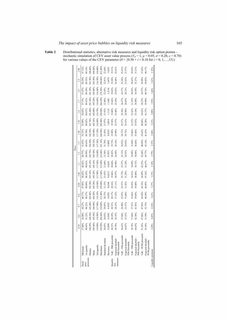
We perform the simulation experiment through constructing a collection of different economies, some with bubbles and some without, by varying the CEV parameter θ from 0.50 to 2.0 in steps of size 0.10. In each of these different economies, we compute the standard risk measures to determine the impact that bubbles have on their values. We fix the other parameters of the simulation in the base case as follows. Asset value Vt is initiated at a normalised value of one V0 = 1, with a drift rate of 5% per annum, μ = 0.05, and a volatility parameter of 20% per annum, σ = 0.20. The liquidity call event is assumed to occur is asset value at the horizon is below the debt threshold of 0.70, Vτ ≤ c = 0.70. The results of our analysis in the base case are tabulated in Table 2 and illustrated in Figure 4. In Table 2, we present the descriptive statistics and quantile loss measures for the reference (or equity price) process and the LROPs against the values of the CEV parameter. Figure 4 plots some key credit loss measures as well as the LROP against the values of the CEV parameter. In the Appendix, Figures A.1 through A.16 plot the paths and distributions of the reference processes.
We can see from the results that all of the standard risk measures decrease as we increase the CEV parameter into the region where we have an asset price bubble, and the LROP decreases monotonically, as this parameter grows. This is driven by a change in the asset value process as θ rises. Note that some features of the asset value distribution are largely unchanged, such as the mean (just a little above 105% across the board with no trend) or the standard deviation (about 21–22% across the board with no trend), as we increase θ. Interestingly, while the median of the distribution reduces mildly relative to the mean as we increase θ (from around 105% to 101%, reflecting the increased right skewness), the normalised skewness of the distribution increases substantially in θ: doubling from 0.3 to 0.6 as we go from CIR to GBM, and then nearly tripling again to 1.6 at θ = 2. Note further that we see increasing asset value skewness in θ even when in the non-bubble region θ ∈ [0.5, 1.0], with skewness doubling from 0.29 to 0.62 going from θ = 0.5 to θ = 1, and then increasing by greater than 1 and a 1/2 times to 1.65 at θ = 2.
The impact of asset price bubbles on liquidity risk measures 165
Table 2 Distributional statistics, alternative risk measures and liquidity risk option premia – stochastic simulation of CEV asset value process (V0 = 1, μ = 0.05, σ = 0.20, c = 0.70) for various values of the CEV parameter (θ = {0.50 + i × 0.10 for i = 0, 1,…,15})
Thet
a
0.50
0.
6 0.
7 0.
8 0.
90
1.00
1.
1 1.
2 1.
3 1.
40
1.50
1.
6 1.
7 1.
8 1.
9 2.
00
Min
imum
37
.80%
42
.08%
44
.27%
46
.17%
47
.85%
49
.42%
48
.42%
48
.57%
51
.93%
55
.33%
55
.99%
56
.65%
57
.73%
57
.47%
58
.39%
57
.12%
1s
t qua
rtile
90
.85%
91
.22%
90
.22%
90
.37%
90
.09%
90
.35%
90
.01%
89
.99%
89
.65%
89
.70%
89
.82%
89
.67%
89
.41%
89
.10%
89
.55%
89
.14%
M
edia
n 10
4.50
%
104.
30%
10
3.40
%10
3.40
%
103.
30%
10
3.10
%10
3.10
%10
2.70
%10
2.50
%10
2.30
%10
1.70
%10
1.80
%
101.
50%
10
1.30
%
101.
30%
100.
80%
Mea
n 10
5.40
%
105.
50%
10
4.90
%10
5.20
%
105.
30%
10
5.20
%10
5.10
%10
5.30
%10
5.10
%10
5.00
%10
5.10
%10
5.00
%
105.
20%
10
5.00
%
105.
20%
104.
80%
3rd
quar
tile
119.
00%
11
8.90
%
117.
90%
118.
10%
11
8.50
%
117.
90%
117.
60%
118.
00%
117.
30%
117.
20%
116.
90%
116.
70%
11
6.80
%
116.
40%
11
6.30
%11
6.00
%M
axim
um
195.
90%
20
2.60
%
210.
80%
215.
40%
25
9.80
%
217.
60%
213.
00%
212.
80%
251.
10%
240.
50%
282.
90%
294.
80%
26
6.20
%
276.
50%
29
6.60
%41
2.40
%St
anda
rd d
evia
tion
20.8
3%
20.8
3%
20.9
5%
20.7
3%
21.3
3%
21.0
3%
21.0
9%
21.5
4%
21.7
8%
21.4
5%
21.9
7%
21.9
2%
22.4
8%
22.4
5%
22.8
1%
22.6
4%
Stoc
k pr
ice
proc
esse
s
Skew
ness
0.
2894
0.
3442
0.
4525
0.
4701
0.
6346
0.
6213
0.
6241
0.
7073
0.
9002
0.
8323
1.
0914
1.
1135
1.
1483
1.
2134
1.
4474
1.
6535
V
aR –
90t
h pe
rcen
tile
20.5
3%
20.2
9%
20.5
3%
20.1
7%
20.3
4%
19.8
6%
20.0
4%
20.0
5%
19.7
3%
19.9
0%
19.5
6%
19.8
0%
19.6
6%
19.6
5%
19.2
0%
19.3
1%
Expe
cted
shor
tfall
–
90th
Per
cent
ile
28.7
0%
28.3
5%
28.3
3%
27.3
2%
27.1
1%
26.9
7%
26.9
0%
26.4
9%
26.1
6%
25.9
0%
25.5
7%
25.4
0%
25.3
0%
25.0
3%
24.4
8%
24.4
1%
VaR
– 9
5th
perc
entil
e 26
.63%
27
.04%
26
.90%
25
.95%
25
.57%
25
.75%
25
.37%
25
.13%
24
.92%
24
.73%
25
.57%
24
.38%
24
.27%
24
.17%
23
.38%
23
.41%
Ex
pect
ed sh
ortfa
ll –
95
th P
erce
ntile
34
.07%
33
.53%
33
.37%
31
.88%
31
.42%
31
.29%
31
.24%
30
.55%
24
.92%
29
.72%
29
.33%
28
.90%
28
.85%
28
.33%
27
.83%
27
.57%
VaR
– 9
9th
perc
entil
e 38
.78%
37
.84%
37
.51%
35
.66%
34
.92%
34
.91%
34
.84%
34
.09%
33
.84%
33
.06%
32
.22%
31
.82%
31
.55%
30
.93%
30
.43%
29
.83%
Ex
pect
ed sh
ortfa
ll –
99
th P
erce
ntile
44
.65%
42
.30%
41
.91%
39
.84%
39
.80%
38
.88%
38
.72%
38
.04%
36
.66%
35
.86%
35
.93%
35
.10%
34
.98%
34
.39%
33
.27%
33
.31%
VaR
– 9
9.9t
h pe
rcen
tile
51.3
6%
47.8
6%
47.5
6%
44.5
0%
44.3
5%
44.0
9%
42.5
3%
42.6
8%
40.0
5%
39.6
2%
40.8
4%
39.6
2%
38.3
5%
38.5
7%
36.9
8%
37.8
2%
Qua
ntile
lo
ss
mea
sure
s
Expe
cted
shor
tfall
–
99.9
th p
erce
ntile
55
.18%
51
.59%
52
.73%
48
.30%
48
.05%
47
.16%
46
.67%
45
.77%
43
.14%
41
.45%
42
.28%
41
.27%
39
.90%
40
.74%
39
.02%
40
.17%
Liqu
idity
pre
miu
m
4.28
%
4.05
%
4.10
%
3.61
%
3.27
%
3.33
%
3.10
%
2.79
%
2.53
%
2.44
%
2.21
%
2.08
%
1.93
%
1.66
%
1.61
%
1.32
%

166 M. Jacobs Jr.
Table 3 Sensitivity analysis of liquidity risk option premia – stochastic simulation of CEV asset value process for various values of the CEV parameter (θ = {0.50 + i × 0.10 for i = 0, 1,…,15})
Thet
a
0.50
0.
60
0.70
0.
80
0.90
1.
00
1.10
1.
20
1.30
1.
40
1.50
1.
60
1.70
1.
80
1.90
2.
00
VaR
– 9
9.9t
h pe
rcen
tile
51.3
6%
47.8
6%
47.5
6%
44.5
0%
44.3
5%
44.0
9%
42.5
3%
42.6
8%
40.0
5%
39.6
2%
40.8
4%
39.6
2%
38.3
5%
38.5
7%
36.9
8%
37.8
2%
Bas
e ca
se
Liqu
idity
pre
miu
m
4.28
%
4.05
%
4.10
%
3.61
%
3.27
%
3.33
%
3.10
%
2.79
%
2.53
%
2.44
%
2.21
%
2.08
%
1.93
%
1.66
%
1.61
%
1.32
%
Liqu
idity
pre
miu
m
4.98
%
4.58
%
4.51
%
3.93
%
4.10
%
3.63
%
3.62
%
2.94
%
3.04
%
2.69
%
2.44
%
2.36
%
2.07
%
1.80
%
1.76
%
1.66
%
Liqu
idity
inte
rval
1
day
Perc
ent c
hang
e fr
om b
ase
16.5
3%
12.9
5%
10.0
9%
8.93
%
25.2
7%
9.05
%
16.7
0%
5.53
%
19.8
9%
10.3
4%
10.7
9%
13.4
7%
7.25
%
8.44
%
9.57
%
25.4
0%
Liqu
idity
pre
miu
m
3.69
%
3.26
%
3.28
%
2.84
%
2.95
%
2.56
%
2.58
%
1.94
%
2.30
%
1.84
%
1.95
%
1.74
%
1.45
%
1.46
%
1.27
%
1.02
%
Liqu
idity
inte
rval
1
mon
th
Perc
ent c
hang
e fr
om b
ase
–13.
75%
–19
.52%
–19.
83%
–21
.17%
–9
.64%
–2
2.95
%–1
6.70
%–3
0.40
%–9
.39%
–2
4.43
%–1
1.43
%–1
6.16
% –
25.0
0% –
12.2
4% –
21.3
0%–2
3.28
%
Liqu
idity
pre
miu
m
3.57
%
3.58
%
3.08
%
2.84
%
2.82
%
2.52
%
2.39
%
2.09
%
2.19
%
2.01
%
1.83
%
1.70
%
1.55
%
1.25
%
1.16
%
1.22
%
Lock
up p
erio
d
1 qu
arte
r Pe
rcen
t cha
nge
from
bas
e –1
6.53
% –
11.5
7%–2
4.79
% –
21.3
6% –
13.7
0%–2
4.21
%–2
3.02
%–2
4.87
%–1
3.54
%–1
7.53
%–1
6.83
%–1
8.18
% –
19.9
3% –
24.4
7% –
28.2
6%–7
.94%
Li
quid
ity p
rem
ium
5.
03%
4.
52%
4.
55%
4.
03%
3.
98%
3.
68%
3.
42%
3.
32%
2.
93%
2.
51%
2.
49%
2.
14%
1.
95%
1.
81%
1.
60%
1.
43%
Lo
ckup
per
iod
4
year
s Pe
rcen
t cha
nge
from
bas
e 17
.51%
11
.40%
11
.11%
11
.84%
21
.63%
10
.74%
10
.38%
19
.10%
15
.47%
2.
87%
12
.70%
3.
03%
1.
09%
8.
86%
–0
.43%
7.
94%
Li
quid
ity p
rem
ium
15
.29%
15
.01%
14
.63%
14
.39%
7.
60%
14
.22%
13
.48%
13
.41%
13
.01%
12
.92%
12
.62%
11
.52%
11
.48%
9.
11%
10
.51%
10
.33%
A
sset
pro
cess
vo
latil
ity 3
0%
Perc
ent c
hang
e fr
om b
ase
257.
45%
270
.29%
257.
26%
299
.03%
132
.55%
327.
79%
334.
54%
381.
16%
413.
26%
430.
17%
472.
38%
453.
87%
494
.20%
448
.95%
552
.61%
680.
42%
Li
quid
ity p
rem
ium
0.
980%
0.
742%
0.
623%
0.
623%
0.
497%
0.
588%
0.
518%
0.
357%
0.
364%
0.
287%
0.
210%
0.
189%
0.
168%
0.
133%
0.
133%
0.
084%
A
sset
pro
cess
vo
latil
ity 1
5%
Perc
ent c
hang
e fr
om b
ase
–77.
09%
–81
.69%
–84.
79%
–82
.72%
–84
.80%
–82.
32%
–83.
30%
–87.
19%
–85.
64%
–88.
22%
–90.
48%
–90.
91%
–91
.30%
–91
.98%
–91
.74%
–93.
65%
Li
quid
ity p
rem
ium
7.
18%
14
.80%
16
.22%
15
.21%
16
.35%
15
.12%
15
.39%
15
.09%
14
.19%
6.
46%
10
.42%
8.
95%
13
.98%
13
.94%
13
.13%
12
.79%
Li
quid
ity c
all
thre
shol
d 80
%
Perc
ent c
hang
e fr
om b
ase
67.7
8%
265.
11%
296.
00%
321
.86%
400
.21%
354.
74%
396.
36%
441.
56%
460.
06%
165.
35%
372.
74%
330.
59%
623
.40%
740
.02%
715
.40%
866.
89%
Li
quid
ity p
rem
ium
0.
7020
% 0
.624
0%0.
4860
% 0
.492
0% 0
.408
0%0.
2880
%0.
186%
0.
2820
%0.
1800
%0.
1440
%0.
1440
%0.
0540
% 0
.060
0% 0
.042
0% 0
.060
0%0.
0060
%
Liqu
idity
cal
l th
resh
old
60%
Pe
rcen
t cha
nge
from
bas
e –8
3.59
% –
84.6
0%–8
8.13
% –
86.3
5% –
87.5
2%–9
1.34
%–9
4.00
%–8
9.88
%–9
2.90
%–9
4.09
%–9
3.47
%–9
7.40
% –
96.8
9% –
97.4
7% –
96.2
7%–9
9.55
%
The impact of asset price bubbles on liquidity risk measures 167
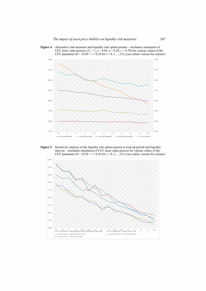
Figure 4 Alternative risk measures and liquidity risk option premia – stochastic simulation of CEV asset value process (V0 = 1, μ = 0.05, σ = 0.20, c = 0.70) for various values of the CEV parameter (θ = {0.50 + i × 0.10 for i = 0, 1,…,15}) (see online version for colours)
Figure 5 Sensitivity analysis of the liquidity risk option premia to lock-up period and liquidity interval – stochastic simulation of CEV asset value process for various values of the CEV parameter (θ = {0.50 + i × 0.10 for i = 0, 1,…,15}) (see online version for colours)
168 M. Jacobs Jr.
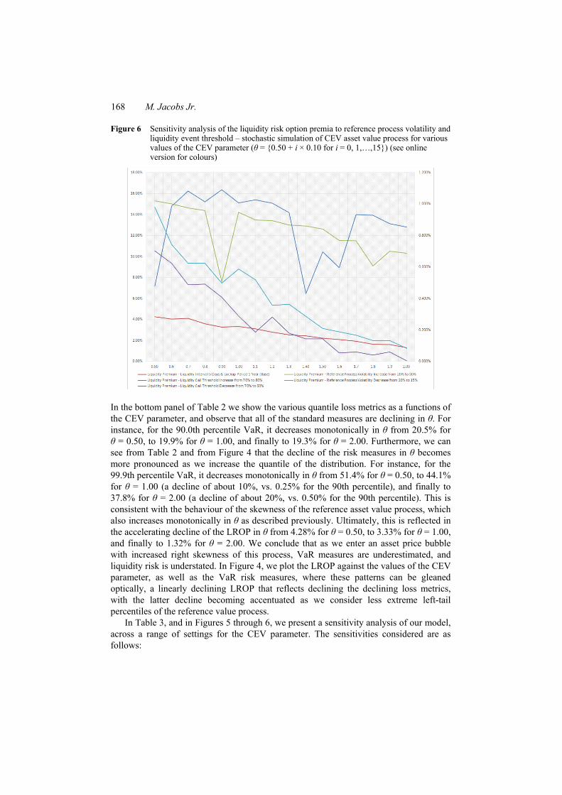
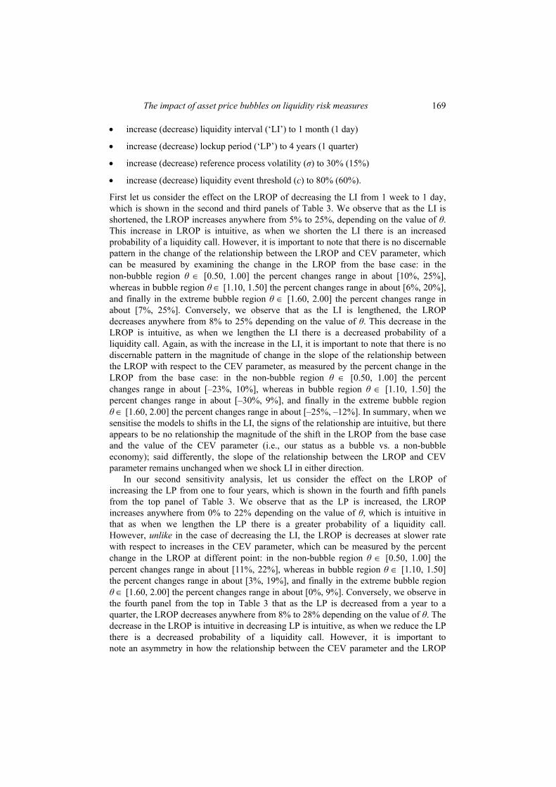
Figure 6 Sensitivity analysis of the liquidity risk option premia to reference process volatility and liquidity event threshold – stochastic simulation of CEV asset value process for various values of the CEV parameter (θ = {0.50 + i × 0.10 for i = 0, 1,…,15}) (see online version for colours)
In the bottom panel of Table 2 we show the various quantile loss metrics as a functions of the CEV parameter, and observe that all of the standard measures are declining in θ. For instance, for the 90.0th percentile VaR, it decreases monotonically in θ from 20.5% for θ = 0.50, to 19.9% for θ = 1.00, and finally to 19.3% for θ = 2.00. Furthermore, we can see from Table 2 and from Figure 4 that the decline of the risk measures in θ becomes more pronounced as we increase the quantile of the distribution. For instance, for the 99.9th percentile VaR, it decreases monotonically in θ from 51.4% for θ = 0.50, to 44.1% for θ = 1.00 (a decline of about 10%, vs. 0.25% for the 90th percentile), and finally to 37.8% for θ = 2.00 (a decline of about 20%, vs. 0.50% for the 90th percentile). This is consistent with the behaviour of the skewness of the reference asset value process, which also increases monotonically in θ as described previously. Ultimately, this is reflected in the accelerating decline of the LROP in θ from 4.28% for θ = 0.50, to 3.33% for θ = 1.00, and finally to 1.32% for θ = 2.00. We conclude that as we enter an asset price bubble with increased right skewness of this process, VaR measures are underestimated, and liquidity risk is understated. In Figure 4, we plot the LROP against the values of the CEV parameter, as well as the VaR risk measures, where these patterns can be gleaned optically, a linearly declining LROP that reflects declining the declining loss metrics, with the latter decline becoming accentuated as we consider less extreme left-tail percentiles of the reference value process.
In Table 3, and in Figures 5 through 6, we present a sensitivity analysis of our model, across a range of settings for the CEV parameter. The sensitivities considered are as follows:
The impact of asset price bubbles on liquidity risk measures 169
• increase (decrease) liquidity interval (‘LI’) to 1 month (1 day)
• increase (decrease) lockup period (‘LP’) to 4 years (1 quarter)
• increase (decrease) reference process volatility (σ) to 30% (15%)
• increase (decrease) liquidity event threshold (c) to 80% (60%).
First let us consider the effect on the LROP of decreasing the LI from 1 week to 1 day, which is shown in the second and third panels of Table 3. We observe that as the LI is shortened, the LROP increases anywhere from 5% to 25%, depending on the value of θ. This increase in LROP is intuitive, as when we shorten the LI there is an increased probability of a liquidity call. However, it is important to note that there is no discernable pattern in the change of the relationship between the LROP and CEV parameter, which can be measured by examining the change in the LROP from the base case: in the non-bubble region θ ∈ [0.50, 1.00] the percent changes range in about [10%, 25%], whereas in bubble region θ ∈ [1.10, 1.50] the percent changes range in about [6%, 20%], and finally in the extreme bubble region θ ∈ [1.60, 2.00] the percent changes range in about [7%, 25%]. Conversely, we observe that as the LI is lengthened, the LROP decreases anywhere from 8% to 25% depending on the value of θ. This decrease in the LROP is intuitive, as when we lengthen the LI there is a decreased probability of a liquidity call. Again, as with the increase in the LI, it is important to note that there is no discernable pattern in the magnitude of change in the slope of the relationship between the LROP with respect to the CEV parameter, as measured by the percent change in the LROP from the base case: in the non-bubble region θ ∈ [0.50, 1.00] the percent changes range in about [–23%, 10%], whereas in bubble region θ ∈ [1.10, 1.50] the percent changes range in about [–30%, 9%], and finally in the extreme bubble region θ ∈ [1.60, 2.00] the percent changes range in about [–25%, –12%]. In summary, when we sensitise the models to shifts in the LI, the signs of the relationship are intuitive, but there appears to be no relationship the magnitude of the shift in the LROP from the base case and the value of the CEV parameter (i.e., our status as a bubble vs. a non-bubble economy); said differently, the slope of the relationship between the LROP and CEV parameter remains unchanged when we shock LI in either direction.
In our second sensitivity analysis, let us consider the effect on the LROP of increasing the LP from one to four years, which is shown in the fourth and fifth panels from the top panel of Table 3. We observe that as the LP is increased, the LROP increases anywhere from 0% to 22% depending on the value of θ, which is intuitive in that as when we lengthen the LP there is a greater probability of a liquidity call. However, unlike in the case of decreasing the LI, the LROP is decreases at slower rate with respect to increases in the CEV parameter, which can be measured by the percent change in the LROP at different point: in the non-bubble region θ ∈ [0.50, 1.00] the percent changes range in about [11%, 22%], whereas in bubble region θ ∈ [1.10, 1.50] the percent changes range in about [3%, 19%], and finally in the extreme bubble region θ ∈ [1.60, 2.00] the percent changes range in about [0%, 9%]. Conversely, we observe in the fourth panel from the top in Table 3 that as the LP is decreased from a year to a quarter, the LROP decreases anywhere from 8% to 28% depending on the value of θ. The decrease in the LROP is intuitive in decreasing LP is intuitive, as when we reduce the LP there is a decreased probability of a liquidity call. However, it is important to note an asymmetry in how the relationship between the CEV parameter and the LROP

170 M. Jacobs Jr.
changes as we change the LP, in that as with shocking the LI in either direction, with the lengthening of the LP there is no clear pattern in the relationship between the magnitude of the increase from the base and the CEV parameter: in the non-bubble region θ ∈ [0.50, 1.00] the percent changes range in about [–25%, –14%], whereas in bubble region θ ∈ [1.10, 1.50] the percent changes range in also about [–25%, –14%] and finally in the extreme bubble region θ ∈ [1.60, 2.00] the percent changes range in about [–28%, –8%]. In summary, when we sensitise the models to shifts in the LP, the signs of the relationship are intuitive, but there appears to be an asymmetry with respect to relationship between the magnitude of the shift and that of the CEV parameter, as when we increase (decrease) the LP there is an inverse relationship (a lack of relationship) to the value of the CEV parameter, or said differently a decrease (no change) in the slope of the relationship.
In our third sensitivity analysis, let us consider the effect on the LROP of shocking the reference process volatility σ, which is shown in the sixth and seventh panels from the top panel of Table 3. When we increase the reference process volatility from 20% to 30%, we observe that in general the LROP increases anywhere from two to seven times depending on the value of θ, which is intuitive, as when we increase reference process volatility there is a greater probability of a liquidity call. However, unlike in the case of the LI or LP sensitivity, in the change in the LROP with respect to increases in the CEV parameter is more pronounced relative to the base case: in the non-bubble region θ ∈ [0.50, 1.00] the percent changes range in about [130%, 330%], whereas in bubble region θ ∈ [1.10, 1.50] the percent changes range in about [330%, 470%], and finally in the extreme bubble region θ ∈ [1.60, 2.00] the percent changes range in about [450%, 680%]. Conversely, we observe in the seventh panel that as σ is decreased from 20% to 15%, in general the LROP decreases anywhere from 77% to 94% depending on the value of θ, which is intuitive as when we reduce σ there is a decreased probability of a liquidity call. Furthermore, the magnitude of the decrease in LROP is increasing with respect to the CEV parameter relative to the base case (although the change in the strength of the relationship is not as robust as for increases in volatility): in the non-bubble region θ ∈ [0.50, 1.00] the percent changes range in about [–85%, –77%], whereas in bubble region θ ∈ [1.10, 1.50] the percent changes range in also about [–90%, –88%] and finally in the extreme bubble region θ ∈ [1.60, 2.00] the percent changes range in about [–94%, –91%]. In summary, when we sensitise the models to shifts in the σ, the signs of the relationship are intuitive, with LROP directly related to the changes in σ. However, unlike the case of LI (for both increases and decreases) or LP (only to the downside), the magnitude of the shift increases in the CEV parameter, although this relationship is stronger with respect to upward as opposed to downward shifts in σ.
In our fourth sensitivity analysis, let us consider the effect on the LROP of shocking the liquidity event threshold c. The impact of the increase from 70% to 80% is shown in the eigth panel from the top panel of Table 3. We observe that as c is increased, in general the LROP increases anywhere from two to nine times depending on the value of θ, which is intuitive, as when we increase the liquidity event threshold there is a greater probability of a liquidity call. As in the case of σ sensitivity, and unlike in the cases of LI (both upward and downward) or LP (to the downside) sensitivity, the change in the LROP relative to base is becoming more pronounced with respect to increases in the CEV parameter: in the non-bubble region θ ∈ [0.50, 1.00] the percent changes range in about [68%, 400%], whereas in bubble region θ ∈ [1.10, 1.50] the LROPs range in about
The impact of asset price bubbles on liquidity risk measures 171
[165%, 460%], and finally in the extreme bubble region θ ∈ [1.60, 2.00] the percent changes range in about [330%, 870%]. However, note that at this level of the c, the LROP is not declining even close to monotonically in the CEV parameter: in the non-bubble region θ ∈ [0.50, 1.00] the LROPs range in about [7%, 16%], whereas in bubble region θ ∈ [1.10, 1.50] the LROPs range in about [6%, 15%], and finally in the extreme bubble region θ ∈ [1.60, 2.00] the LROPs range in about [9%, 14%]. Conversely, we observe in the bottom panel that as c is decreased from 70% to 60%, in general the LROP decreases anywhere from 86% to 100% depending on the value of θ, which is intuitive as when we reduce c there is a decreased probability of a liquidity call. Furthermore, the magnitude of the decrease in LROP from base is increasing with respect to the CEV parameter (although the strength of the relationship is not as robust as for decreases in volatility): in the non-bubble region θ ∈ [0.50, 1.00] the percent changes range in about [–91%, –84%], whereas in bubble region θ ∈ [1.10, 1.50] the percent changes range in about [–94%, –90%] and finally in the extreme bubble region θ ∈ [1.60, 2.00] the percent changes range in about [–100%,–96%]. In summary, when we sensitise the models to shifts in the c, the signs of the relationship are intuitive, with LROP directly related to the changes in c. Furthermore, as with the case in shocking σ, the magnitude of the shift relative to the base case increases in the CEV parameter, although this relationship is stronger with respect to upward as opposed to downward shifts in c.
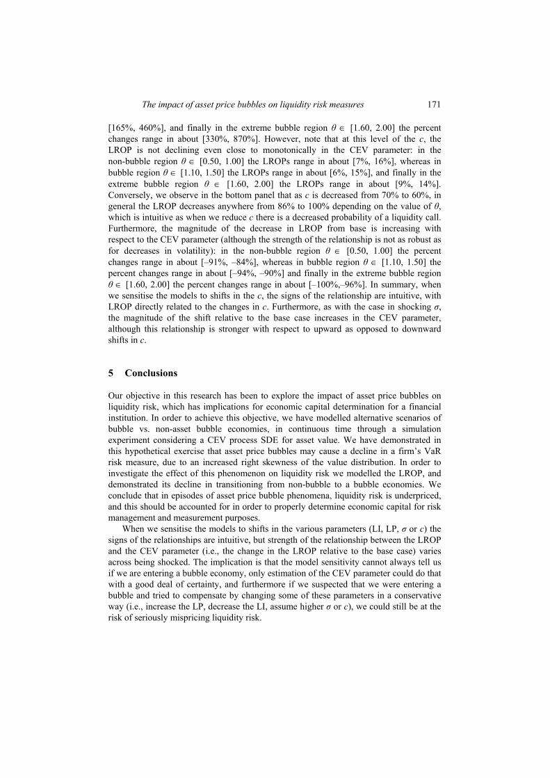
5 Conclusions
Our objective in this research has been to explore the impact of asset price bubbles on liquidity risk, which has implications for economic capital determination for a financial institution. In order to achieve this objective, we have modelled alternative scenarios of bubble vs. non-asset bubble economies, in continuous time through a simulation experiment considering a CEV process SDE for asset value. We have demonstrated in this hypothetical exercise that asset price bubbles may cause a decline in a firm’s VaR risk measure, due to an increased right skewness of the value distribution. In order to investigate the effect of this phenomenon on liquidity risk we modelled the LROP, and demonstrated its decline in transitioning from non-bubble to a bubble economies. We conclude that in episodes of asset price bubble phenomena, liquidity risk is underpriced, and this should be accounted for in order to properly determine economic capital for risk management and measurement purposes.
When we sensitise the models to shifts in the various parameters (LI, LP, σ or c) the signs of the relationships are intuitive, but strength of the relationship between the LROP and the CEV parameter (i.e., the change in the LROP relative to the base case) varies across being shocked. The implication is that the model sensitivity cannot always tell us if we are entering a bubble economy, only estimation of the CEV parameter could do that with a good deal of certainty, and furthermore if we suspected that we were entering a bubble and tried to compensate by changing some of these parameters in a conservative way (i.e., increase the LP, decrease the LI, assume higher σ or c), we could still be at the risk of seriously mispricing liquidity risk.

172 M. Jacobs Jr.
Acknowledgements
The views expressed herein are those of the authors and do not necessarily represent a position taken either by Accenture, or of any affiliated firms.
References Acharya, V., Philippon, T., Richardson, M. and Roubini, N. (2009) ‘The financial crisis of
2007–2009: causes and remedies’, Financial Markets, Institutions & Instruments, Vol. 18, pp.89–137.
Alexander, C. (2001) Market Models: A Guide to Financial Data Analysis, Wiley, New York, NY. Back, K. (2010) Asset Pricing and Portfolio Choice Theory, Oxford University Press, London, UK. Baretsky, P., Gruber, W. and When, C. (Eds.) (2008) Handbuch Liquiditatrisiko: Identification,
Messung und Steuerung, Schlaffel-Poeschel Verlag, Stuttgart. Basel Committee on Banking Supervision (BCBS) (2005) An Explanatory Note on the Basel II IRB
Risk Weight Functions, Bank for International Settlements, July. Basel Committee on Banking Supervision (BCBS) (2006) International Convergence of Capital
Measurement and Capital Standards: A Revised Framework, June, Bank for International Settlements.
Basel Committee on Banking Supervision (BCBS) (2009a) Principles for Sound Stress Testing Practices and Supervision – Consultative Paper, May (No. 155).
Basel Committee on Banking Supervision (BCBS) (2009b) Strengthening the Resilience of the Banking Sector, December, Bank for International Settlements Consultative Document.
Basel Committee on Banking Supervision (BCBS) (2010) Basel III: A Global Regulatory Framework for More Resilient Banks and Banking Systems, December, Bank for International Settlements.
Chan, K.C., Karolyi, G.A., Longstaff, F.A. and Saunders, A.B. (1992) ‘An empirical comparison of various models of the short-term interest rate’, Journal of Finance, Vol. 47, No. 3, pp.1209–1227.
Cornford, A. (2005) Basel II: The Revised Framework of June 2004, Technical Report, United Nations Conference on Trade and Development.
Delbaen, F. and Schachermayer, W. (1995) ‘Arbitrage possibilities in Bessel processes and their relations to local martingales’, Probability Theory and Related Fields, Vol. 102, No. 3, pp.357–366.
Delbaen, F. and Schachermayer, W. (1998) ‘The fundamental theorem of asset pricing for unbounded stochastic processes’, Mathematische Annalen, Vol. 312, No. 2, pp.215–250.
Demirguc-Kunt, A. and Serven, L. (2010) ‘Are all the sacred cows dead? Implications of the financial crisis for macro- and financial policies’, World Bank Research Observer, February, Vol. 25, No. 1, pp.91–124.
Duttweiler, R. (2008) ‘Liquidititat als Teil der bankbetreibswirtschaftlichen Finanzpolitik’, in Bartezsky, P., Gruber, W. and When, C. (Eds.): Handbuch Liquiditatrisiko: Identification, Messung und Steuerung, pp.29–50, Schlaffel-Poeschel Verlag, Stuttgart.
Emanuel, D.C. and MacBeth, J.D. (1982) ‘Further results on the constant elasticity of variance call option pricing model’, Journal of Financial and Quantitative Analysis, Vol. 17, No. 4, pp.533–554.
Embrechts, P., Lindskog, F. and McNeil, A.J. (2003) ‘Modeling dependence with copulas and applications to risk management’, in Rachev, S. (Ed.): Handbook of Heavy Tailed Distributions in Finance, pp.329–384, Elsevier, Rotterdam.
Embrechts, P., McNeil, A.J. and Straumann, D. (1999) ‘Correlation: pitfalls and alternatives’, Risk, Vol. 12, No. 3, pp.69–71.

The impact of asset price bubbles on liquidity risk measures 173
Embrechts, P., McNeil, A.J. and Straumann, D. (2002) ‘Correlation and dependence in risk management: properties and pitfalls’, in Dempster, M.A.H. (Ed.): Risk Management: Value at Risk and Beyond, pp.176–223, Cambridge University Press, Cambridge, UK.
Engelmann, B. and Rauhmeier, R. (2006) The Basel II Risk Parameters, Springer, New York, NY. Fielder, R. (2007) ‘A concept for cash flow and funding liquidity risk’, in Matz, L. and Neu, P.
(Eds.): Liquidity Risk: Measurement and Management, pp.173–203, John Wiley & Sons, Singapore.
Frey, R. and McNeil, A.J. (2001) Modeling Dependent Defaults, Working Paper, ETH Zurich. Golts, M. and Kritzman, M. (2010) ‘Liquidity options (April 5, 2010)’, Journal of Derivatives,
Vol. 18, No. 1, Revere Street Working Paper Series No. 272-27 [online] SSRN: http://ssrn.com/abstract=1584857 or http://dx.doi.org/10.2139/ssrn.1584857 (accessed 15 September 2015).
Hiedorn, T. and Schamlz, C. (2008) ‘Neue Entwicklungen der Liquiditatsmanagement’, in Bartezky, P., Gruber, W. and When, C. (Eds.): Handbuch Liquiditatrisiko: Identifikation, Messung und Steurung, pp.193–229, Schaffer-Poeschel Verlag, Stuttgart.
Hong, H., Scheinkman, J. and Xiong, W. (2006) ‘Asset float and speculative bubbles’, Journal of Finance, Vol. 61, No. 3, pp.1073–1117.
Inanoglu, H. and Jacobs Jr., M. (2009) ‘Models for risk aggregation and sensitivity analysis: an application to bank economic capital’, The Journal of Risk and Financial Management, Vol. 2, No. 4, pp.118–189.
Inanoglu, H., Jacobs Jr., M., Liu, J. and Sickles, R.C. (2015) ‘Analyzing bank efficiency: are “too-big-to-fail” banks efficient?’, in Haven, E.E. (Ed.): Handbook of Post Crisis Financial Modelling, March, Palgrave Macmillan, New York.
Jacobs Jr., M. (2001) A Comparison of Fixed Income Valuation Models: Pricing and Econometric Analysis of Interest Rate Derivatives, Unpublished Doctoral Dissertation, The Graduate School and University Center of the City University of New York.
Jacobs Jr., M. (2013) ‘Stress testing credit risk portfolios’, Journal of Financial Transformation, April–March, Vol. 37, pp.53–75.
Jacobs Jr., M. (2015) ‘The impact of asset price bubbles on credit risk measures’, Journal of Financial Risk Management, Vol. 4, pp.251–266.
Jacobs Jr., M., Karagozoglu, A.K. and Sensenbrenner, F.J. (2015) ‘Stress testing and model validation: application of the Bayesian approach to a credit risk portfolio’, The Journal of Risk Model Validation, Vol. 9, No. 3, pp.41–70.
Jarrow, R.A. and Protter, P. (2010) ‘The martingale theory of bubbles: implications for the valuation of derivatives and detecting bubbles’, in Berd, A. (Ed.): The Financial Crisis: Debating the Origins, Outcomes, and Lessons of the Greatest Economic Event of Our Lifetime, pp.429–448, Risk Publications, London, UK.
Jarrow, R.A. and Silva, F.B.G. (2014) ‘Risk measure and the impact of asset price bubbles’, Journal of Risk, Vol. 17, No. 3, pp.35–56.
Jarrow, R.A., Kchia, Y. and Protter, P. (2011) ‘How to detect an asset bubble’, SIAM Journal on Financial Mathematics, Vol. 2, No. 1, pp.839–865.
Jarrow, R.A., Protter, P. and Shimko, K. (2007) ‘Asset price bubbles in complete markets’, in Fu, M.C., Jarrow, R.A., Yen, J-Y.J. and Elliott, R.J. (Eds.): Advances in Mathematical Finance, pp.97–121, Springer, New York.
Jarrow, R.A., Protter, P. and Shimko, K. (2010a) ‘Asset price bubbles in incomplete markets*’, Mathematical Finance, Vol. 20, No. 2, pp.145–185.
Jarrow, R.A., Protter, P. and Shimko, K. (2010b) ‘Risk measures and the impact of asset price bubbles’, Journal of Risk, Vol. 17, No. 3, pp.35–55.
Jeanblanc, M., Yor, M. and Chesney, M. (2009) Mathematical Methods for Financial Markets, Springer, New York, NY.

174 M. Jacobs Jr.
Jorion, P. (1997) Value at Risk: The New Benchmark for Controlling Market Risk, Vol. 2, McGraw-Hill, New York.
Jorion, P. (2006) Value at Risk: The Benchmark for Managing Financial Risk, 3rd ed., McGraw Hill, New York, NY.
Knies, K. (1876) Geld und Credit II, Abteilung Der Credit, Leipzig. Li, D.X. (2000) ‘On default correlation: a copula function approach’, Journal of Fixed Income,
Vol. 9, No. 4, pp.43–54. Matz, L. (2002) Liquidity Risk Management, Thompson/Sheshunoff, Austin, TX. Merton, R. (1974) ‘On the pricing of corporate debt: the risk structure of interest rates’, Journal of
Finance, Vol. 29, No. 2, pp.449–470. Øksendal, B.K. (2003) Stochastic Differential Equations: An Introduction with Applications,
6th ed., Springer, Berlin. Poon, S-H., Rockinger, M. and Tawn, J. (2004) ‘Extreme value dependence in financial
markets: diagnostics, models and financial implications’, Review of Financial Studies, Vol. 17, No. 2, pp.581–610.
Protter, P. (2011) ‘How to detect an asset bubble’, SIAM Journal on Financial Mathematics, Vol. 2, No. 1, pp.839–865.
Reitz, S. (2008) ‘Moderne Konzepte zur Liquiditatrisikos’, in Bartezky, P., Gruber, W. and When, C. (Eds.): Handbuch Liquiditatrisiko: Identifikation, Messung und Steurung, pp.121–140, Schaffer-Poeschel Verlag, Stuttgart.
R Development Core Team (2015) R: A Language and Environment for Statistical Computing, R Foundation for Statistical Computing, Vienna, Austria, ISBN 3-900051-07-0.
Schroder, M. (1989) ‘Computing the constant elasticity of variance option pricing formula’, Journal of Finance, Vol. 44, No. 1, pp.211–219.
Sklar, A. (1956) Fonctions de répartition à n dimensions et leurs marges, pp.229–231, Publications de l’Institut de Statistique de L’Université de Paris 8.
Stutzel, W. (1959) ‘Liquiditat’, in von Beckerath, E. (Ed.): Handworterbuch der Socialwisenschaft, Stuttgart.
The U.S. Board of Governors of the Federal Reserve System (2011) Supervisory Guidance on Model Risk Management (OCC 2011-12).
Notes 1 For applications of the CEV model in finance see Chan et al. (1992) and Jacobs (2001), in the
context of term structure and interest rate derivatives. 2 In the wake of the financial crisis (Demirguc-Kunt and Serven, 2010; Acharya et al., 2009),
international supervisors have recognised the importance of stress testing (ST), especially in the realm of credit risk, as can be seen in the revised Basel framework (BCBS, 2005, 2006, 2009a, 2009b) and the Federal Reserve’s Comprehensive Capital Analysis and Review (‘CCAR’) program (Jacobs, 2013; Jacobs et al., 2015).
3 The conditions are that τ* is almost surely increasing * *1[ ] 1Q
k kP τ τ +< = and is almost surely divergent *[ as ] 1Q
kP τ k→∞ →∞ = (Oksendal, 2003).
4 This condition is sometimes termed ‘no free-lunch with vanishing risk’ or NFLVR (Jeanblanc et al., 2009).
5 This is partly due to the Basel II Accords (Engelmann and Rauhmeier, 2006; Cornford, 2005). 6 We use the R package Sim.DiffProc to simulate the two-dimensional system of SDEs for asset
value and for LGD (R Development Core Team, 2015)
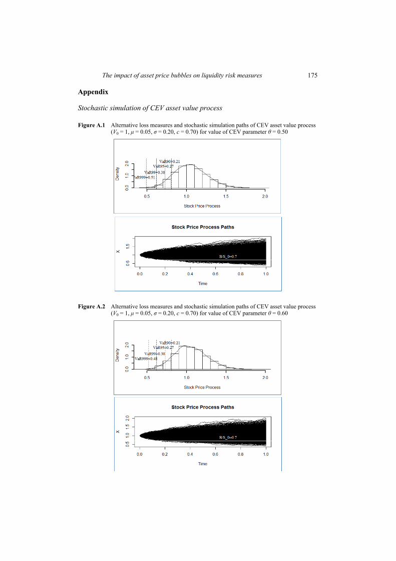
The impact of asset price bubbles on liquidity risk measures 175
Appendix
Stochastic simulation of CEV asset value process
Figure A.1 Alternative loss measures and stochastic simulation paths of CEV asset value process (V0 = 1, μ = 0.05, σ = 0.20, c = 0.70) for value of CEV parameter θ = 0.50
Figure A.2 Alternative loss measures and stochastic simulation paths of CEV asset value process (V0 = 1, μ = 0.05, σ = 0.20, c = 0.70) for value of CEV parameter θ = 0.60
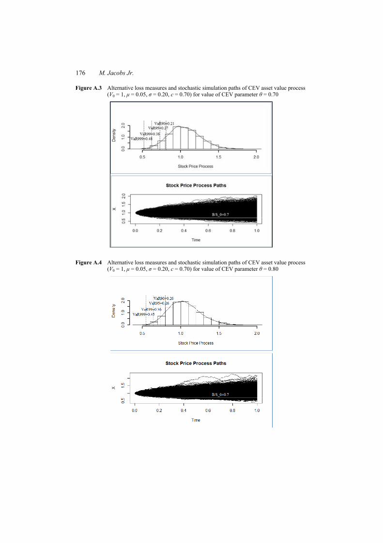
176 M. Jacobs Jr.
Figure A.3 Alternative loss measures and stochastic simulation paths of CEV asset value process (V0 = 1, μ = 0.05, σ = 0.20, c = 0.70) for value of CEV parameter θ = 0.70
Figure A.4 Alternative loss measures and stochastic simulation paths of CEV asset value process (V0 = 1, μ = 0.05, σ = 0.20, c = 0.70) for value of CEV parameter θ = 0.80

The impact of asset price bubbles on liquidity risk measures 177
Figure A.5 Alternative loss measures and stochastic simulation paths of CEV asset value process (V0 = 1, μ = 0.05, σ = 0.20, c = 0.70) for value of CEV parameter θ = 0.90
Figure A.6 Alternative loss measures and stochastic simulation paths of CEV asset value process (V0 = 1, μ = 0.05, σ = 0.20, c = 0.70) for value of CEV parameter θ = 1.00

178 M. Jacobs Jr.
Figure A.7 Alternative loss measures and stochastic simulation paths of CEV asset value process (V0 = 1, μ = 0.05, σ = 0.20, c = 0.70) for value of CEV parameter θ = 1.10
Figure A.8 Alternative loss measures and stochastic simulation paths of CEV asset value process (V0 = 1, μ = 0.05, σ = 0.20, c = 0.70) for value of CEV parameter θ = 1.20

The impact of asset price bubbles on liquidity risk measures 179
Figure A.9 Alternative loss measures and stochastic simulation paths of CEV asset value process (V0 = 1, μ = 0.05, σ = 0.20, c = 0.70) for value of CEV parameter θ = 1.30
Figure A.10 Alternative loss measures and stochastic simulation paths of CEV asset value process (V0 = 1, μ = 0.05, σ = 0.20, c = 0.70) for value of CEV parameter θ = 1.40
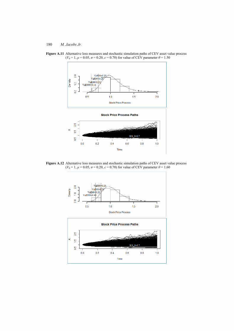
180 M. Jacobs Jr.
Figure A.11 Alternative loss measures and stochastic simulation paths of CEV asset value process (V0 = 1, μ = 0.05, σ = 0.20, c = 0.70) for value of CEV parameter θ = 1.50
Figure A.12 Alternative loss measures and stochastic simulation paths of CEV asset value process (V0 = 1, μ = 0.05, σ = 0.20, c = 0.70) for value of CEV parameter θ = 1.60
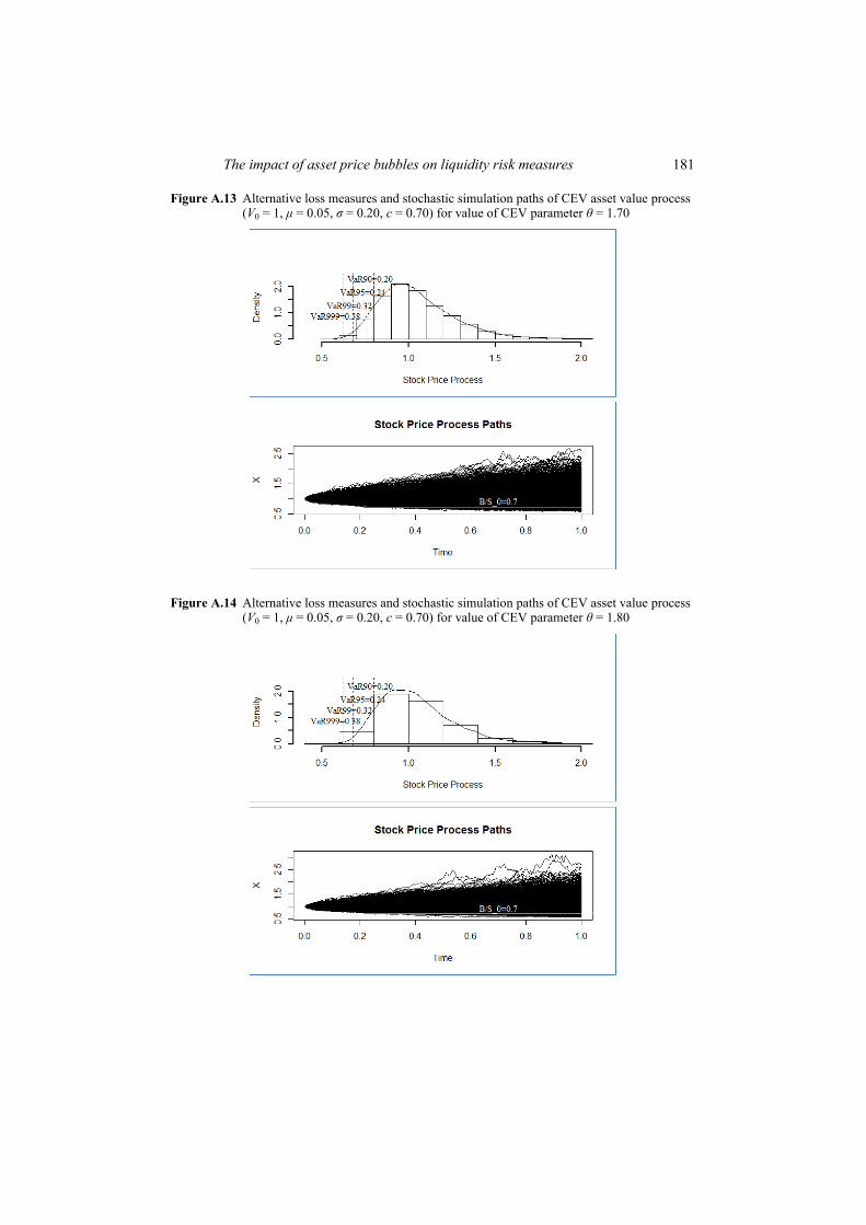
The impact of asset price bubbles on liquidity risk measures 181
Figure A.13 Alternative loss measures and stochastic simulation paths of CEV asset value process (V0 = 1, μ = 0.05, σ = 0.20, c = 0.70) for value of CEV parameter θ = 1.70
Figure A.14 Alternative loss measures and stochastic simulation paths of CEV asset value process (V0 = 1, μ = 0.05, σ = 0.20, c = 0.70) for value of CEV parameter θ = 1.80
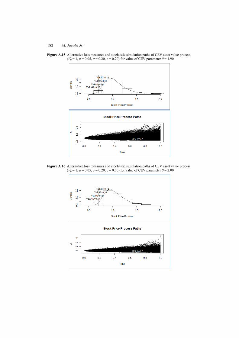
182 M. Jacobs Jr.
Figure A.15 Alternative loss measures and stochastic simulation paths of CEV asset value process (V0 = 1, μ = 0.05, σ = 0.20, c = 0.70) for value of CEV parameter θ = 1.90
Figure A.16 Alternative loss measures and stochastic simulation paths of CEV asset value process (V0 = 1, μ = 0.05, σ = 0.20, c = 0.70) for value of CEV parameter θ = 2.00