The Iceberg Theory of Campaign Contributions: Political ...econweb.umd.edu/~kaplan/jmp_final.pdf ·...
31
1 American Economic Journal: Economic Policy 2013, 5(1): 1–31 http://dx.doi.org/10.1257/pol.5.1.1 The Iceberg Theory of Campaign Contributions: Political Threats and Interest Group Behavior † By Marcos Chamon and Ethan Kaplan* We present a model where special interest groups condition contribu- tions on the receiving candidate’s support and also her opponent’s. This allows interest groups to obtain support from contributions as well as from threats of contributing. Out-of-equilibrium contribu- tions help explain the missing money puzzle. Our framework con- tradicts standard models in predicting that interest groups give to only one side of a race. We also predict that special interest groups will mainly target lopsided winners, whereas general interest groups will contribute mainly to candidates in close races. We verify these predictions in FEC data for US House elections from 1984–1990. (JEL D72) G rowing concerns about the increasing role of money in politics, and the influ- ence of interest groups on policy, are voiced with unerring regularity in popular and policy debates (Lessig 2011). Much of those concerns have not found support in the empirical literature on campaign contributions. While there is a widespread popular perception that there is too much money in politics, researchers, beginning with Tullock (1972), have struggled to rationalize why there is actually so little money considering the value of the favors campaign contributions allegedly buy. The sugar industry provides an excellent illustration of this point. The sugar program provides subsidies and huge tariff and non-tariff protection to US producers. The General Accounting Office estimates that the sugar program led to a net gain of over $1 billion to the sugar industry in 1998 (General Accounting Office 2000). However, the total combined contributions across sugar industry political action committees (PACs) in the two years of that election cycle were a mere $2.8 million (1.5 thousandths of the * Chamon: International Monetary Fund, 700 19th ST NW, Washington, DC 20431 (e-mail:mchamon@imf. org); Kaplan: Department of Economics, University of Maryland at College Park, 3105 Tydings Hall, College Park, MD 20742 (e-mail: [email protected]). We are grateful to David Austen-Smith, Stephen Coate, Ernesto Dalbo, Irineu de Carvalho Filho, Stefano Della Vigna, Gene Grossman, David Lee, Richard Lyons, Rob McMillan, Nicola Persico, Torsten Persson, David Romer, Gerard Roland, Noah Schierenbeck, David Stromberg, and seminar participants at Cambridge University, Columbia University, Cornell University, Dartmouth College, the Federal Reserve Bank of New York, the Graduate Institute for International Studies (Geneva), Gothenburg University, the Institute for International Economic Studies (Stockholm University), Harvard/MIT Political Economy Seminar, New York University, Northwestern University, Tel Aviv University, University of California at Berkeley, the University of Oslo, the 2004 Meeting of the European Economic Association, and two referees for helpful com- ments. Sebastien Turban provided excellent research assistance. Any errors are ours. Mr. Chamon began this paper prior to joining the IMF staff and completed it outside of his IMF duties. The IMF did not sponsor his work on the paper and takes no position on the topics it discusses. † To comment on this article in the online discussion forum, or to view additional materials, visit the article page at http://dx.doi.org/10.1257/pol.5.1.1.
Transcript of The Iceberg Theory of Campaign Contributions: Political ...econweb.umd.edu/~kaplan/jmp_final.pdf ·...
1
American Economic Journal: Economic Policy 2013, 5(1): 1–31 http://dx.doi.org/10.1257/pol.5.1.1
The Iceberg Theory of Campaign Contributions: Political Threats and Interest Group Behavior†
By Marcos Chamon and Ethan Kaplan*
We present a model where special interest groups condition contribu-tions on the receiving candidate’s support and also her opponent’s. This allows interest groups to obtain support from contributions as well as from threats of contributing. Out-of-equilibrium contribu-tions help explain the missing money puzzle. Our framework con-tradicts standard models in predicting that interest groups give to only one side of a race. We also predict that special interest groups will mainly target lopsided winners, whereas general interest groups will contribute mainly to candidates in close races. We verify these predictions in FEC data for US House elections from 1984–1990. (JEL D72)
Growing concerns about the increasing role of money in politics, and the influ-ence of interest groups on policy, are voiced with unerring regularity in popular
and policy debates (Lessig 2011). Much of those concerns have not found support in the empirical literature on campaign contributions. While there is a widespread popular perception that there is too much money in politics, researchers, beginning with Tullock (1972), have struggled to rationalize why there is actually so little money considering the value of the favors campaign contributions allegedly buy. The sugar industry provides an excellent illustration of this point. The sugar program provides subsidies and huge tariff and non-tariff protection to US producers. The General Accounting Office estimates that the sugar program led to a net gain of over $1 billion to the sugar industry in 1998 (General Accounting Office 2000). However, the total combined contributions across sugar industry political action committees (PACs) in the two years of that election cycle were a mere $2.8 million (1.5 thousandths of the
* Chamon: International Monetary Fund, 700 19th ST NW, Washington, DC 20431 (e-mail:[email protected]); Kaplan: Department of Economics, University of Maryland at College Park, 3105 Tydings Hall, College Park, MD 20742 (e-mail: [email protected]). We are grateful to David Austen-Smith, Stephen Coate, Ernesto Dalbo, Irineu de Carvalho Filho, Stefano Della Vigna, Gene Grossman, David Lee, Richard Lyons, Rob McMillan, Nicola Persico, Torsten Persson, David Romer, Gerard Roland, Noah Schierenbeck, David Stromberg, and seminar participants at Cambridge University, Columbia University, Cornell University, Dartmouth College, the Federal Reserve Bank of New York, the Graduate Institute for International Studies (Geneva), Gothenburg University, the Institute for International Economic Studies (Stockholm University), Harvard/MIT Political Economy Seminar, New York University, Northwestern University, Tel Aviv University, University of California at Berkeley, the University of Oslo, the 2004 Meeting of the European Economic Association, and two referees for helpful com-ments. Sebastien Turban provided excellent research assistance. Any errors are ours. Mr. Chamon began this paper prior to joining the IMF staff and completed it outside of his IMF duties. The IMF did not sponsor his work on the paper and takes no position on the topics it discusses.
† To comment on this article in the online discussion forum, or to view additional materials, visit the article page at http://dx.doi.org/10.1257/pol.5.1.1.
2 AmEriCAn ECOnOmiC JOUrnAL: ECOnOmiC POLiCy FEBrUAry 2013
net gain from the sugar program). Ansolabehere, de Figueiredo, and Snyder (2003) discuss a number of other similar examples.
The empirical literature has had mixed success in finding systematic evidence of an effect of contributions on policy outcomes. Much of that literature, reviewed in detail in Ansolabehere, de Figueiredo, and Snyder (2003), has focused on the effect of contributions on roll call voting behavior. Though some studies do find significant correlation for specific industries or for contributions by individuals (Mian, Sufi, and Trebbi 2010), a large fraction of studies do not indicate a statistically significant effect. Goldberg and Maggi (1999) estimate a structural model that captures the effect of industry contributions on their nontariff barriers coverage ratio based on the canonical Grossman and Helpman (1994) framework. They estimate that policymakers would be willing to forsake $98 of contributions to avoid a $1 loss of social welfare. The lack of systematic evidence of an effect of contributions on policy has led some to conclude that contributions are small precisely because they do not affect the political process much. Examples include Ansolabehere, de Figueiredo, and Snyder (2003) and Milyo, Primo, and Groseclose (2000).
In this paper, we present a framework that reconciles the existing empirical lit-erature with the popular view that there is too much influence of special interests in politics. Campaign contributions have traditionally been thought of as transactions involving only the contributor and the receiving candidate or political party. Such a perspective largely ignores how the possibility of contributing to an opponent could also affect the patterns of contributions and support. Unlike the previous literature, we allow interest groups to announce schedules of contributions which are contin-gent not only on the platform of the candidate receiving the offer (bilateral contact-ing) but also on the platform of the opposing candidate (multilateral contracting). As a result, a candidate may support a special interest not only in order to receive a contribution, but also in order to discourage that special interest from making a contribution to his or her opponent. This leverages the power of special interests, whose influence may be driven, or at least leveraged, by implicit out-of-equilibrium contributions, generating a disconnect between their influence and the actual con-tributions we observe. This approach also explains a number of empirical patterns documented in this paper which standard models cannot.
Our model of electoral competition builds on the frameworks of Grossman and Helpman (1996) and Baron (1994). Two candidates compete for office. Voters base their choice on the candidates’ platforms and an “impression” component that is influenced by campaign expenditures. We consider two types of interest groups: special interest groups and general interest groups. Special interest groups care only about a particular policy, and do not care inherently about which candidate wins the election as long as their special interest policy is supported by the winner. As in Baron (1994), campaign contributions can “buy” some of the impressionable component of the vote, but catering to special interests will cost the candidates votes amongst the informed component of the vote. General interest groups, on the other hand, care about a policy dimension over which voters are divided and over which politicians are precommitted, so they do care about which candidate gets elected. They contribute mainly in close elections in order to increase the odds that a candi-date they prefer gets elected.
VOL. 5 nO. 1 3Chamon and Kaplan: The ICeberg Theory of CampaIgn ConTrIbuTIons
In our multilateral contracting framework, a special interest group’s threat of contributing $1 dollar to the opponent can induce the same level of support to the special interest policy as an actual $1 dollar contribution to each candidate would in a bilateral contracting setting. Even when equilibrium contributions are made, they are still leveraged by an implicit out-of-equilibrium threat. For example, sup-pose a special interest group contributes $2,000 to the stronger of two candidates in exchange for its support, while threatening to contribute $10,000 to her opponent if that support is denied. This $2,000 equilibrium contribution in our multilateral contracting framework can induce the same level of support from that candidate that a $12,000 would in a traditional bilateral contracting setting ($2,000 for the actual contribution and $10,000 for the out-of-equilibrium one). Similarly, the weaker can-didate will provide a level of support to the special interest policy similar to that obtained by an $8,000 contribution in a bilateral contracting setting (the difference between the $10,000 the special interest can threaten to contribute to the opponent and the $2,000 it actually does). Thus, the $2,000 equilibrium contributions merely scratch the surface, with out-of-equilibrium contributions 9 times as large helping to “buy” support to the special interest without money actually being spent. Even if we considered only the contributions to the stronger candidate in this example, the spe-cial interest would still have leveraged its equilibrium contribution with out-of-equi-librium contributions 5 times as large. As equilibrium contributions get smaller, that leverage gets larger because more money is left in reserves for threats. For example, if the special interest contributes only $1,000 then out-of-equilibrium contributions to that candidate would be 10 times larger than equilibrium contributions, and for a $500 equilibrium contribution that ratio would be 20. We show, through a simple back-of-the-envelope calculation, that under reasonable assumptions on the number of contributors and the size of the legislature, our framework is capable of explain-ing very large rates of return (as large as those enjoyed by the sugar industry). This framework also has interesting and counterintuitive implications for campaign finance reform. Stricter limits on campaign contributions make out-of-equilibrium threats less effective, raising the marginal return to equilibrium contributions. As a result, stricter limits can actually lead to an increase in equilibrium contributions, but will always weaken interest group influence.
Many papers have tried to explain the missing money puzzle. Ansolabehere, de Figueiredo, and Snyder (2003) suggest that contributions are for consumption value. A large literature beginning with Gopoian (1984) and Poole, Romer, and Rosenthal (1987) views interest groups as trying to influence election outcomes rather than policies. However, neither of these strands of the literature explain why support levels for interest groups are so high nor do they explain why contributions are often larger in lopsided races than in close races. Other models have altered the timing of moves, allowing interest groups to move after politicians, or made stylized assump-tions about agenda-setting power in the legislative process. Dal Bó (2007); Fox and Rothenberg (2010); Grossman and Helpman (2001); Helpman and Persson (2001); and Persson and Tabellini (2000) are the closest models to our own in that they allow out-of-equilibrium ex post contributions to drive support for a policy favorable to an interest group. These models are able to explain a high degree of support for spe-cial interests. However, these models share the prediction that no contributions will
4 AmEriCAn ECOnOmiC JOUrnAL: ECOnOmiC POLiCy FEBrUAry 2013
occur in equilibrium. Our model is the first to show that an interest group may make both equilibrium and out-of-equilibrium contributions simultaneously, and that the degree to which each is used will depend on the candidate’s electoral strength. That is, our multilateral contracting approach allows for the possibility of out-of-equilib-rium contributions without leading to a collapse in equilibrium contributions, pro-viding an explanation for the “missing money” puzzle while still explaining why contributions actually are made and particularly to candidates that are more likely to win. As such, we can make a plausible empirical case for an explanation of the miss-ing money puzzle. In addition, our model also predicts that interest groups never give to both sides of a race, since the same level of support from each candidate can be achieved with less contributions when they are “one-sided” (for example, the support stemming from a $2,000 contribution to the stronger candidate and a $1,000 contribution to the weaker one could be achieved by just contributing $1,000 to the former). This prediction is strongly supported in the data. The few other models that also predict one-sided contributions are ones with proposal power such as Helpman and Persson (2001); however, these models also typically predict that most candi-dates, even lopsided winners, get zero contributions.
The model’s empirical predictions are tested using data from US House elec-tions in 1984–1990. We use itemized contributions data from the Federal Election Commission (FEC) to classify PACs as partisan or nonpartisan based on whether their contributions fall within a 75–25 percent split between the two major parties. The partisan contributors are analogous to the general interest groups in our model, while nonpartisan contributors are analogous to the special interest groups. The data indicates that while it is common for special interest groups to contribute to candi-dates from both parties, they very rarely contribute to opposing candidates in the same race, consistent with our model (and contradicting standard models which typically predict “two-sided” contributions). Finally, the predicted pattern whereby special interest groups contribute mainly to lopsided winners whereas general inter-est groups contribute mainly to close election candidates is also verified in the data.
The remainder of this paper is organized as follows: Section I presents a model of electoral competition with interest group influence. Sections II and III characterize campaign contribution patterns for general interest groups and special interest groups, respectively. Section IV presents empirical evidence confirming the predictions of the model. Section V discusses policy implications. Finally, Section VI concludes.
I. The Model
Our basic setting builds on the framework of Grossman and Helpman (1996). We assume that there are three strategic actors in the game: two candidates competing in a legislative race and one interest group. We separately consider two types of inter-est groups: general (or partisan) interest groups and special (or nonpartisan) interest groups. There are two stages of the model. First, the interest group moves, offer-ing payments in exchange for policy commitments by candidates. Unlike previous models, we allow special interest groups to condition payments to a given candidate, not only on her platform but also on that of her opponent. In the second stage, the two candidates simultaneously choose their levels of support for the interest group
VOL. 5 nO. 1 5Chamon and Kaplan: The ICeberg Theory of CampaIgn ConTrIbuTIons
policy, contributions are made, and payoffs are received. We assume that candi-dates have ideological preferences over certain general interest policy issues. These preferences are commonly known, and despite what candidates may say during a campaign, they will vote according to their fixed preferences once elected. However, we assume they can commit their position on a “pliable” special interest policy.1
A. Voters
For expositional purposes, we first present a model of electoral competition with-out interest groups. Following Baron (1994) and Grossman and Helpman (1996), each voter makes her decision based not only upon what policies candidates will implement, but also on her “impression” which is influenced by the amount of money spent on campaigns. We consider a median-voter type model, where voters have single-peaked preferences over the candidate’s fixed policy and over the pli-able policies. The “informed” component of the vote is based on the voter’s prefer-ence for one candidate’s platform over the other. That preference is determined by the differences in the candidates’ positions on the fixed policy plus the difference in the candidates’ positions on the pliable policy.
We focus on the voting decision of the median voter since her ballot is decisive. We denote her preference for candidate A by b + ϵ, where b is the average ideo-logical bias of the population in favor of candidate A and ϵ is the realization of a mean zero shock to ideology. The realization of ϵ is distributed with a continuous, symmetric, single-peaked distribution of unbounded support. Thus, in the absence of pliable policies or campaign expenditures, the probability that the median voter prefers candidate A (and therefore the probability that candidate A wins the election) is given by
P(b + ϵ > 0) = 1 − F(− b),
where F(− b) is the cumulative distribution of ϵ evaluated at − b. However, vot-ers also care about pliable policies. The median voter’s utility function is given by b + ϵ + W(τ) where W(τ) is the voter utility over the pliable policy, τ, of the winning candidate. Special interest pliable policies are assumed to be uniformly disliked by all voters:
(1) ∂ W(τ) _ ∂ τ < 0.
Also, for convenience of mathematical notation, we assume that W(0) = 0 and define τ , the pliable policy of interest to the special interest group, over [0, ∞).
Finally, the popularity of the candidates is also altered by campaign spend-ing. Any given voter is more likely to support candidate A over B the higher the
1 As in Grossman and Helpman (1996; 2001, 69).
6 AmEriCAn ECOnOmiC JOUrnAL: ECOnOmiC POLiCy FEBrUAry 2013
difference between the expenditures by A and B. We denote campaign expenditures by candidate k as m k . The median voter casts a ballot for candidate A when
b + ϵ + W( τ A ) − W( τ B ) + m A − m B > 0.
The probability that the median voter casts her ballot for candidate A (and there-fore candidate A wins the election) is given by2
∫ −[b+W( τ A )−W( τ B )+ m A − m B ]
∞
f (ϵ)d ϵ = 1 − F[− b − (W( τ A ) − W( τ B ) + m A − m B )].
We also sometimes refer to 1 − F[− b − (W( τ A ) − W( τ B ) + m A − m B )] as the probability of candidate A winning: P(A).
B. Candidates
The expected utility of candidate k, where k ∈ {A, B} is equal to the probability of winning:
U k = P(k).
Our results are robust to the introduction of other components in the candidate’s utility, such as an added utility over pliable policies or from money balances which are not spent on the campaign.
C. interest Groups
Finally, we turn to interest groups. We consider two types: special (or nonpar-tisan) interest groups and general (or partisan) interest groups. Special interest groups (SIGs) care only about a special interest policy τ and money. These groups are nonpartisan in the sense that they do not care about the ideology or party affili-ation of the winner, just about the resulting policy τ. Examples would include the sugar industry and other industry-specific lobbies, lobbies for government pro-curement such as specific military contractors, and trade policy lobbies. General interest groups (GIGs) care about policies over which candidates have fixed pref-erences. In other words, they have preferences over policies that candidates are unable to commit to support (or to not support) once in office. These groups will be partisan in the sense that they will prefer the winning candidate to be the one with similar fixed preferences. Examples of GIGs would include tax policy inter-est groups, labor groups, the gun lobby, pro-choice and pro-life groups, among others. We first analyze electoral competition with one GIG and then turn to a
2 As is standard, we denote by f the probability density function of ϵ. Note that if the bias b towards candidate A is zero, and both candidates announce the same pliable policies and have the same level of expenditures the prob-ability of candidate A winning the election is exactly 1/2.
VOL. 5 nO. 1 7Chamon and Kaplan: The ICeberg Theory of CampaIgn ConTrIbuTIons
setting with one SIG. We do not analyze a setting with both SIGs and GIGs though that could be an interesting extension.
The utility function for the SIG is thus defined as
U SiG = P(A) W SiG ( τ A ) + [1 − P(A)] W SiG ( τ B ) + m SiG − m A − m B ,
where W SiG ( τ k ) is the value to the SIG of implementing policy τ k and m SiG is the amount of money held by the SiG. We assume that SIGs like higher levels of pol-icy:
∂ W SiG ( τ k ) _ ∂ τ k
> 0 and that W SiG (0) = 0. We also assume
m SiG ∈ [0, ∞)
m A , m B ∈ [0, _ m ]
τ A , τ B ∈ [0, ∞),
where _ m is the legal limit on interest group campaign contributions to a candidate.
In addition, we define a variable which will be useful in our analysis. Let θ(τ) be the ratio of the marginal utility to the SIG to the marginal disutility caused to voters of an increase in the special interest policy:
(2) ∂ W SiG (τ) _ ∂ τ = − θ(τ) ∂ W(τ) _ ∂ τ .
We assume that at higher levels of special interest policy, voters care weakly more on the margin about the policy relative to interest groups3:
∀ τ : ∂ θ(τ) _ ∂ τ ≤ 0.
In the particular case of the GIG, politicians policy positions are fixed. We write the objective function of the GIG as
U GiG = P(A) + m GiG − m A − m B ,
where m GiG is the money held by the GIG. We further assume that m GiG ∈ [0, ∞).
3 We motivate this assumption with reference to a tariff model with incomplete information where voters infer policy changes from prices whereas businesses explicitly follow policy. For small policy changes, voters can’t dis-tinguish between small policy changes and random fluctuations in prices but firms can.
8 AmEriCAn ECOnOmiC JOUrnAL: ECOnOmiC POLiCy FEBrUAry 2013
II. General Interest Group
In this section, we look at the patterns of contributions that arise when there is one general interest group. Without loss of generality, we assume that the general inter-est group is ideologically aligned with candidate A. Therefore, it tries to maximize a weighted sum of the probability of candidate A’s victory and money balance after contributions. We write the formal maximization problem as
max { m A , m B }
1 − F[− b − m A + m B ] + m GiG − m A − m B
s.t.: 0 ≤ m A , m B ≤ _ m , m A + m B ≤ m GiG .
An equilibrium of the game is given by a vector of scalars specifying contribu-tions by the interest group such that the above problem is maximized:
[ m A * , m B * ].
Grossman and Helpman (1996) make a useful distinction between two types of motives for contributions: an influence motive, whereby contributions seek to influ-ence the candidate’s platforms, and an electoral motive, whereby contributions seek to influence the outcome of the election taking the platforms as given. The GIG will never contribute to the ideologically opposing candidate because the candidate cannot credibly commit to change her ideology. In lopsided elections, the GIG will not con-tribute any money to the race. In close elections, there is an electoral motive for giving to the candidate with which the GIG is aligned.
PROPOSITION 1: GiGs never give money to ideologically opposing candidates and give to aligned candidates only in sufficiently close elections.
PROOF: See Appendix.
The intuition of this result is quite simple. For close elections, the interest group spends money on improving candidate A’s victory prospects. The interest group is willing to spend money as long as the value of doing so is greater than the oppor-tunity cost of alternative usage of the funds. When the distribution of voter prefer-ences is single peaked and symmetric, marginal shifts in probability of victory per dollar spent will be highest (and thus contributions will occur) in close races. This is encapsulated in the following formula for the Kuhn-Tucker-Lagrange (KTL) multi-plier on non-negativity of contributions to party A ( λ A ):
− λ A = f (− b + m A − m B ) − 1 + λ GiG + λ _ m A ,
VOL. 5 nO. 1 9Chamon and Kaplan: The ICeberg Theory of CampaIgn ConTrIbuTIons
where λ GiG is the KTL for the GIG’s budget constraint, and λ _ m A is the KTL on contributions to candidate A not being greater than legal contribution limits. Since the KTL multiplier on non-negativity of contributions to candidate A is the value of relaxing the constraint on not reducing contributions by a dollar below zero, − λ A can roughly be interpreted as the marginal value of donating when campaign contribution limits and budget constraints don’t bind. This is then equal to the marginal gain in probability of electoral victory for the candidate preferred by the interest group less the marginal value of the dollar. Moreover, the marginal value of contribution may be even higher when the budget constraint of the interest group or campaign contribution limits are binding.
III. Special Interest Group
Whereas general interest groups mainly contribute to candidates in close elec-tions in order to affect the outcome of the election, this sub-section shows that special interest groups contribute to lopsided winners in order to influence the pol-icies which the likely winner implements; in close races, special interest groups rely more heavily on out of equilibrium threats. Since special interest groups are trying to influence candidates in areas where candidates can make commit-ments, they can condition their payments on what the candidates announce. In Proposition 1 of the online Appendix, we show that we can represent the SIG’s maximization problem as a contract theory problem where the SIG maximizes its utility choosing policy support levels for candidates A and B and monetary support levels for candidates A and B, subject to individual rationality (IR) constraints for the two candidates. Since the SIG’s maximization problem is a full information problem, there is no incentive compatibility constraint. Therefore, the contract theory representation reduces to choosing the proper IR constraint. The most that the SIG can harm a candidate is to give all the money it is capable of giving to the opposing candidate without requiring additional policy support. Moreover, since threats never materialize in equilibrium, there is no cost to the SIG from making the maximum possible threat. For example, candidate A’s outside option is given by candidate B maintaining her equilibrium level of support for the SIG, but can-didate A supporting at level zero, and thus the SIG giving the maximum amount possible to candidate B:
U A [ τ A * , τ B * , m A * , m B * ] ≥ U A [0, τ B * , 0, min [ _ m , m SiG ]].
This stands in contrast to a bilateral contracting model where the amount given to candidate B would have to be the same in candidate A’s inside option and outside option. Then the IR constraint would be: U A [ τ A * , τ B * , m A * , m B * ] ≥ U A [0, τ B * , 0, m B * ]. If the SIG has less money than the contribution cap, then the maximum amount which the SIG can use to threat a candidate is m SiG ; otherwise, it is
_ m . In order
to simplify our expressions, we make the innocuous and empirically motivated assumption that interest group coffers are larger than campaign contribution caps:
_ m ≤ m SiG .
10 AmEriCAn ECOnOmiC JOUrnAL: ECOnOmiC POLiCy FEBrUAry 2013
Formulated as a contract theory problem, the only difference between bilat-eral and multilateral contracting reduces to whether or not the amount of money given to the opponent in the inside option of the individual rationality constraint equals the amount given in the outside option. The SIG’s maximization problem is given by
(3)
max τ A , τ B , m A , m B U SiG [ τ A , τ B , m A , m B ]
s.t.: U A [ τ A , τ B , m A , m B ] ≥ U A [0, τ B , 0, _ m ]
U B [ τ A , τ B , m A , m B ] ≥ U B [ τ A , 0, _ m , 0]
0 ≤ m A , m B ≤ _ m , m A + m B ≤ m SiG .
The first implication of our multilateral contracting framework is that the SIG will never contribute to both sides of the same race. The intuition behind our result is simple. Suppose that when the SIG gives ( m A , m B ) to candidates A and B, it achieves support levels ( τ A , τ B ). Further assume, without loss of generality, that m A > m B . With bilateral offers, a reduction in contributions to either candidate means a reduc-tion in support from that candidate. However, with multilateral offers, the SIG can give m B dollars less to candidate A and compensate her by giving m B dollars less to candidate B. Similarly, the lower contribution to candidate B is fully compensated by the lower contribution to candidate A. Thus, the SIG could offer ( m A − m B , 0) while still maintaining support levels ( τ A , τ B ) and keeping 2 m B extra dollars. The SIG will never give positive amounts to both candidates. One-sidedness of contribu-tions is one of the key distinguishing predictions of our model when compared with standard models in the literature, which typically predict two-sided contributions (e.g., Snyder 1990 or Grossman and Helpman 1996).
PROPOSITION 2: SiGs never give to both sides in the same race.
PROOF: See Appendix.
For notational simplicity, let Δ = − b − (W( τ A ) − W( τ B ) + m A − m B ). We now characterize when contributions to a candidate are positive. We do this by deriving a formula for the Lagrange multipliers on non-negativity of contributions to candidates. Contributions to a candidate are zero when the multiplier is positive. We also show that outside options always bind. Using the fact that outside options bind, we then use the Lagrange multipliers to characterize when contributions are positive as a function of the probability a candidate has of winning.
In a bilateral contracting model, an interest group may choose to give more money to a supportive candidate than necessary in order to increase that candidate’s chances of electoral victory. In the multilateral contracting version, this cannot happen. The SIG can instead keep the extra money and by keeping it, increase support from the
VOL. 5 nO. 1 11Chamon and Kaplan: The ICeberg Theory of CampaIgn ConTrIbuTIons
opposing candidate. This would leave the odds of electoral victory for the supportive candidate unchanged while increasing support from the opposing candidate. As such, it is always preferable. We thus prove that outside options always bind:
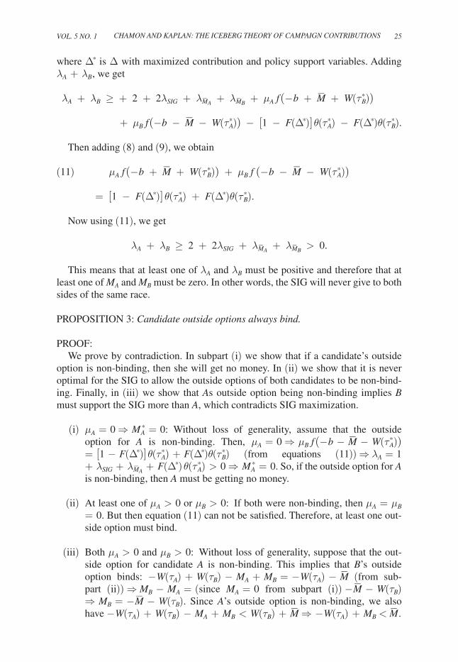
PROPOSITION 3: Candidate outside options always bind.
PROOF: See Appendix.
In the Appendix, we derive the following characterization of the KTL multipliers λ A and λ B associated with the non-negativity of contributions to A and B respectively:
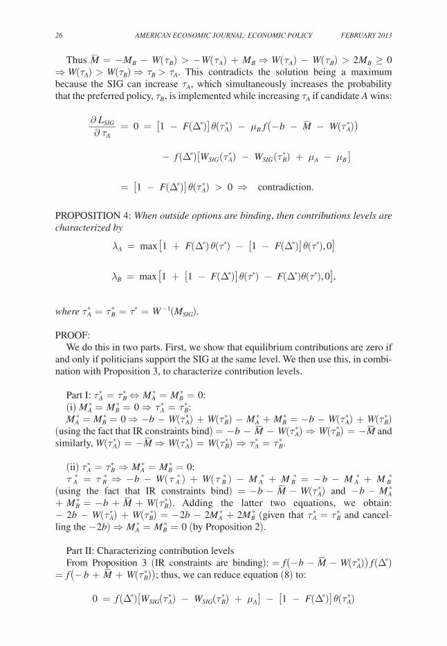
PROPOSITION 4: When outside options are binding, then contributions levels are characterized by:
λ A = max [1 + F(Δ) θ(τ) − [1 − F(Δ)] θ(τ), 0]
λ B = max [1 + [1 − F(Δ)] θ(τ) − F(Δ)θ(τ), 0],
where τ A = τ B = τ = W −1 ( _ m ).
PROOF: See Appendix.
The intuition is relatively simple. If the outside options for candidate B binds, the gross marginal benefit of contributing to A is the benefit the SIG obtains from additional support from candidate A: [1 − F(Δ)] θ( τ A ). The gross marginal cost of contributing to A is equal to the loss in the SIG’s ability to threaten candi-date B, given by F(Δ) θ( τ B ), plus the direct marginal disutility of contributing money (equal to 1). That gross marginal benefit outweighs the gross marginal cost only if A is sufficiently strong. Since outside options always bind, the charac-terization of λ A , λ B always holds. We can therefore use our formulas for λ A , λ B to state our characterization of contribution patterns for the Special Interest Group. The SIG contributes when one of λ A , λ B is not positive. This happens when either F(Δ) − [1 − F(Δ)] is sufficiently negative or F(Δ) − [1 − F(Δ)] is sufficiently positive. In other words, this happens when the vote margin difference between the candidates is sufficiently large:
PROPOSITION 5: The SiG always receives equilibrium support from at least one candidate but contributes only in sufficiently lopsided races.
PROOF: See Appendix.
Out-of-equilibrium threats lead to a collapse in contributions when both λ A and λ B are positive (so the constraints on the non-negativity of contributions bind). The range of
12 AmEriCAn ECOnOmiC JOUrnAL: ECOnOmiC POLiCy FEBrUAry 2013
F(Δ) for which that is the case is ( 1 _ 2 − 1 _
2θ(τ) , 1 _ 2 + 1
_ 2θ(τ) ), which becomes arbitrarily
small when interest groups care much more intensively about the special interest policy in comparison with the average voter: θ(τ) → ∞.
An interest group has two possible schedules of offers to make: distributed and concentrated threats. Either the interest group can use a prisoner’s dilemma type game to get an equal amount of support from each of the candidates or it can con-centrate the threats on one candidate, making the schedule only a function of what that candidate announces. In the concentrated threats schedule, for low levels of support from a candidate, the SIG threatens to contribute to the opposing candidate and for high levels of support, the SIG makes direct contributions to the candidate in question. The relative benefits of making equilibrium contributions (the concen-trated threats offer) will be high when the difference in the probability of winning is sufficiently high that even with the loss in direct utility from holding money by the SIG, the SIG still prefers to concentrate threats rather than spread them around.
We now present a simple example which is analytically tractable and illustrates the basic results of our model. By making sensible functional form choices, we are able to solve for the amount of contributions and support levels rather than just characterizing when equilibrium contributions are made. We assume that voter utility over special interest policy is equal to W( τ k ) = − τ k , and that the interest group cares more about the policy compared to voters: W SiG ( τ k ) =
_ θ τ k , where
_ θ > > 1. We deviate slightly
from the baseline model by choosing the distribution of ϵ to be uniform: U[− K, K]4 We assume that the amount of money which the interest group is able to spend is suf-ficiently low that, given the initial bias in favor of candidate A, b, even if the interest group gave all its money away without asking for any policy support in return, neither party would win with 100 percent probability. This condition reduces to: b +
_ m < K
and − b − _ m < − K. We additionally assume K ≥ (
_ θ _ m )/(
_ θ − 1) to ensure that
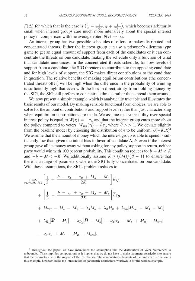
there is a range of parameters where the SIG fully concentrates on one candidate. With these assumptions, the SIG’s problem reduces to:
max τ A , τ B , m A , m B
[ 1 _ 2 + b − τ A + τ B + m A − m B
___ 2K
] _ θ τ A
+ [ 1 _ 2 − b − τ A + τ B + m A − m B
___ 2K
] _ θ τ B
+ m SiG − m A − m B + λ A m A + λ B m B + λ SiG [ m SiG − m A − m B ]
+ λ _ m A [ _ m − m A ] + λ _ m B [
_ m − m B ] − ν A [ τ A − m A + m B − m SiG ]
− ν B [ τ B + m A − m B − m SiG ].
4 Throughout the paper, we have maintained the assumption that the distribution of voter preferences is unbounded. This simplifies computations as it implies that we do not have to make parameter restrictions to ensure that the parameters lie in the support of the distribution. The computational benefits of the uniform distribution in this example, however, make the introduction of parametric restrictions worthwhile for the worked example.
VOL. 5 nO. 1 13Chamon and Kaplan: The ICeberg Theory of CampaIgn ConTrIbuTIons
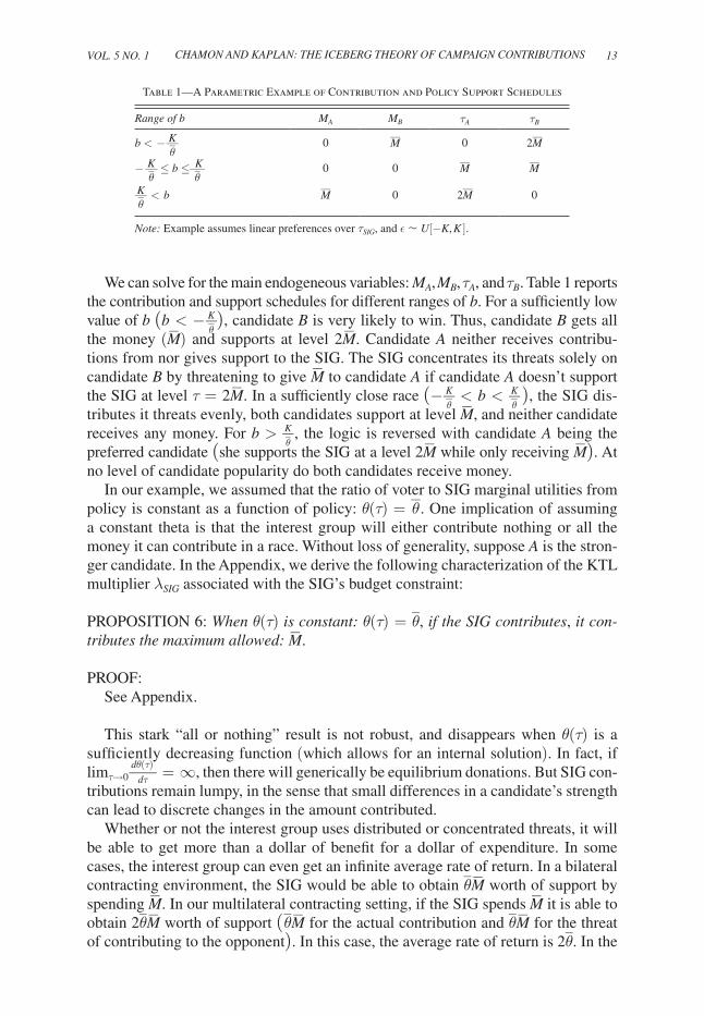
We can solve for the main endogeneous variables: m A , m B , τ A , and τ B . Table 1 reports the contribution and support schedules for different ranges of b. For a sufficiently low value of b (b < − K _
_ θ ), candidate B is very likely to win. Thus, candidate B gets all
the money ( _ m ) and supports at level 2
_ m . Candidate A neither receives contribu-
tions from nor gives support to the SIG. The SIG concentrates its threats solely on candidate B by threatening to give
_ m to candidate A if candidate A doesn’t support
the SIG at level τ = 2 _ m . In a sufficiently close race (− K _
_ θ < b < K _
_ θ ), the SIG dis-
tributes it threats evenly, both candidates support at level _ m , and neither candidate
receives any money. For b > K _ _ θ , the logic is reversed with candidate A being the
preferred candidate (she supports the SIG at a level 2 _ m while only receiving
_ m ). At
no level of candidate popularity do both candidates receive money.In our example, we assumed that the ratio of voter to SIG marginal utilities from
policy is constant as a function of policy: θ(τ) = _ θ . One implication of assuming
a constant theta is that the interest group will either contribute nothing or all the money it can contribute in a race. Without loss of generality, suppose A is the stron-ger candidate. In the Appendix, we derive the following characterization of the KTL multiplier λ SiG associated with the SIG’s budget constraint:
PROPOSITION 6: When θ(τ) is constant: θ(τ) = _ θ , if the SiG contributes, it con-
tributes the maximum allowed: _ m .
PROOF: See Appendix.
This stark “all or nothing” result is not robust, and disappears when θ(τ) is a sufficiently decreasing function (which allows for an internal solution). In fact, if li m τ→0
dθ(τ) _
dτ = ∞, then there will generically be equilibrium donations. But SIG con-tributions remain lumpy, in the sense that small differences in a candidate’s strength can lead to discrete changes in the amount contributed.
Whether or not the interest group uses distributed or concentrated threats, it will be able to get more than a dollar of benefit for a dollar of expenditure. In some cases, the interest group can even get an infinite average rate of return. In a bilateral contracting environment, the SIG would be able to obtain
_ θ _ m worth of support by
spending _ m . In our multilateral contracting setting, if the SIG spends
_ m it is able to
obtain 2 _ θ _ m worth of support (
_ θ _ m for the actual contribution and
_ θ _ m for the threat
of contributing to the opponent). In this case, the average rate of return is 2 _ θ . In the
Table 1—A Parametric Example of Contribution and Policy Support Schedules
range of b mA mB τA τB
b < − K _ _ θ 0
_ m 0 2
_ m
− K _ _ θ ≤ b ≤ K _
_ θ 0 0
_ m
_ m
K _ _ θ < b
_ m 0 2
_ m 0
note: Example assumes linear preferences over τSiG, and ϵ ~ U[−K, K ].
14 AmEriCAn ECOnOmiC JOUrnAL: ECOnOmiC POLiCy FEBrUAry 2013
opposite extreme where the SIG spends no money, it gets _ θ _ m worth of support from
each candidate. In this case, it gets an infinite rate of return (although the value of the support obtained is bounded and the optimal strategy for the interest group is not necessarily the one that maximizes the rate of return):
PROPOSITION 7: When θ(τ) is constant, the average rate of return to money con-tributed by the SiG ranges from 2
_ θ to ∞.
PROOF: See Appendix.
The leverage provided by out-of-equilibrium threats in our model immediately suggests a quantitatively relevant explanation for the missing money puzzle. We do a back of the envelope calculation of the potential strength of this leverage, using the sugar industry as an illustration. We do this by computing the rate of return to total contributions (equilibrium plus out of equilibrium). In doing so, we assume that the sugar industry coordinates and acts as a single interest group with a limitation on spending equal to the number of PACs multiplied by the limitation on giving by an individual PAC.
The General Accounting Office estimated the benefits to the sugar industry gen-erated by the sugar program to be $1 billion in 1998 (at a cost of $2 billion to US consumers, General Accounting Office 2000). In the 1998 electoral cycle, the sugar industry contributed $2.8 million; this corresponds to 1.5 thousandths of the favors received during that time, since each electoral cycle covers two years. The sugar industry contributed $2 million to Congressional candidates. Most of the remain-ing $800 thousand were likely soft money contributions, with $1.4 million going to House races. They contributed with a 52–48 percent split favoring Democrats, mak-ing it a “textbook” example of an SIG. There were 17 sugar-related PACs, which together contributed $1.6 million to congressional races, $1.2 million of which went to House candidates.5 These 17 PACs retained $800 thousand on reserve. If the entirety of the reserves could be used as an out-of-equilibrium threat to the stronger candidate in each of the 435 House races, out-of-equilibrium contributions would correspond to 435 multiplied by $800,000 or $348 million. This number would increase to $375 million if we also included the 34 Senate races. If we also consider out-of-equilibrium contributions to losing candidates, these figures would roughly double6, making them comparable to the benefits received by the sugar industry.
In practice, the magnitude of out-of-equilibrium contributions is limited by cam-paign finance rules, which impose a $10,000 cap unless they are made through inde-pendent expenditures or issue ads, in which case there would not be a limit. Out of the 17 PACs, 11 had at least $10,000 on reserves. If each of these 11 threatened to contrib-ute the maximum of $10,000 and the other six didn’t attempt to have any influence, the amount available on reserves to the opponent of a candidate that did not support
5 The campaign contribution figures reported in this section are based on data for the sugar industry available at www.opensecrets.org.
6 They would not exactly double since there are uncontested races.
VOL. 5 nO. 1 15Chamon and Kaplan: The ICeberg Theory of CampaIgn ConTrIbuTIons
the sugar special interest, then each House election winner would have faced $10,000 multiplied by 11 PACS. In other words, each House winner would have faced $110 thousand in out-of-equilibrium contributions, which would add up to $110,000 multi-plied by 435 or $48 million in the 435 House races. This corresponds to 40 times the amount of equilibrium contributions made by those PACs in House races. Thus, the ratio of value of favors allegedly bought to total contributions declines from about one thousand to one down to about ten to one if we consider both in and out-of-equilibrium contributions. This still holds despite the strong restrictions imposed on the size of contributions. That ratio can be further lowered if the number of potential contributors increases. For example, presumably the six PACs with less than $10,000 on reserves could have raised more money if sufficiently inclined to do so, and there is likely a number of individuals with a sufficiently large stake in the sugar program that would be willing to make a large contribution against a candidate opposing the program.
Our framework suggests that organized industries with low levels of contribu-tions may be compensating with greater use of out-of-equilibrium threats, since observed contributions may not be strongly correlated with policy outcomes (e.g., Goldberg and Maggi 1999). This could explain the disconnect between contribu-tions and influence observed in the empirical literature. Unorganized industries, on the other hand, may not be as able to influence policy.
IV. Empirical Evidence
The multilateral contracting approach presented in this paper makes many predic-tions. First, it implies that interest groups, including those with influence motives for donating, will not give to both sides of the same race. Second, it implies that a candidate will receive more SIG money the more likely she is to win an election. Third, it implies that GIGs will give more to candidates engaged in close elections. In this section, these prediction are all verified using itemized contribution data from the Federal Elections Commission (FEC). In addition, we provide anecdotal evidence that interest groups do threaten to contribute to opposing candidates in order to extract concessions.
A. Data
All individual contributions of $200 or more as well as contributions made by a committee are required to be reported to the Federal Election Commission (FEC). Data files itemizing those contributions are available through the FEC website, which also provides information on election results. Committees which raise and spend money to elect and defeat candidates are referred to as PACs. Following most of the literature on campaign contributions, we focus our analysis on US House general election races, and on contributions by PACs which are not connected to a party.7 We use data from the US House elections in 1984–1990. We focus on that earlier sample because soft money, which cannot be traced to particular candidates, and independent expenditures
7 Their contribution pattern is more varied than that of party committees and individuals, and seems more relevant for interest group considerations. A previous version of this paper also considered contributions by party committees and by individuals. Their behavior matched the pattern of contributions of GIGs, as one would expect.
16 AmEriCAn ECOnOmiC JOUrnAL: ECOnOmiC POLiCy FEBrUAry 2013
played a relatively smaller role then.8 Our results are similar if we include data from the 1990s and 2000s as well. For comparison purposes, contributions data is inflated to 2010 prices using the Consumer Price Index.
We construct a measure of partisanship for each PAC, in each election cycle, based on the share of its contributions to Democrat and Republican House candi-dates. We ignore independent or third-party candidates. PACs which give more than 25 percent but less than 75 percent of their contributions to both major parties are classified as SIGs. PACs which give 75 percent or more of their contributions to one party are classified as GIGs.9 We drop independent expenditures, which by law must be made without consultation, coordination or cooperation with the supported candidate or party. These expenditures are relatively small vis-à-vis the contribu-tions considered in our sample, and their inclusion does not change the qualitative results presented. The PAC contributions considered account for about 40 percent of the total contributions received by the candidates with the remaining coming from either individuals or party committees. SIGs account for about 55 percent of the contributions in our sample, with GIGs accounting for the remaining share.
Under the election laws that were applicable during our sample, in each cycle PACs were allowed to contribute at most $5,000 per candidate per election (pri-mary and general elections count as separate elections), $5,000 per other PAC and $15,000 per national party committee, and did not face any limits on total contribu-tions.10 In practice, there were ways through which an interest group could contrib-ute beyond those limits.11
B. results
The first prediction of our multilateral contracting approach is the “one-sided-ness” of contributions. If an SIG were to contribute $2,000 to a Democrat House candidate and $1,000 to her Republican opponent, the SIG would have been able to achieve a similar level of support by contributing only $1,000 to the Democrat and nothing to the Republican. Hence $2,000 worth of contributions in the former sce-nario would be “redundant.” In more formal terms, if giver g contributes m g, D j to the Democrat candidate in race j, and m g, r j to the Republican candidate in that race, then
Redundanc y g, j = 2 · min ( m g, D j , m g, r j ).
8 See http://www.citizen.org/documents/killingussoftlyreport.pdf.9 We experimented with a variety of different cutoff levels for the definitions of SIG and GIG, ranging from very
strict (e.g., SIGs contributing at most 60 percent to one party) to very lax (e.g., SIGs contributing at most 90 percent to one party). Since SIGs target mainly stronger candidates, they tend to give more to the majority party, which is the one with more lopsided winners on average. We also experimented with SIG definitions based on whether the interest group’s share of contributions to a party were inside a 25 percent band around that party’s share of the House in that year. The results are qualitatively similar across all these different rules.
10 Figures refer to “multi-candidate” committees. Otherwise, the limits were $1,000, $5,000, and $20,000 respectively.
11 One notable circunvention was “soft money” contributions, which in theory were meant to be raised by party organizations for non-federal election purposes. They were eliminated after the 2002 election cycle. Since soft money contributions cannot be traced to a specific giver-candidate pairing, they are not used in our analysis. The FEC data only identifies soft money contributions when they started to rise in importance. Beginning with the 1992 cycle, they accounted for 16 percent of all contributions.
VOL. 5 nO. 1 17Chamon and Kaplan: The ICeberg Theory of CampaIgn ConTrIbuTIons
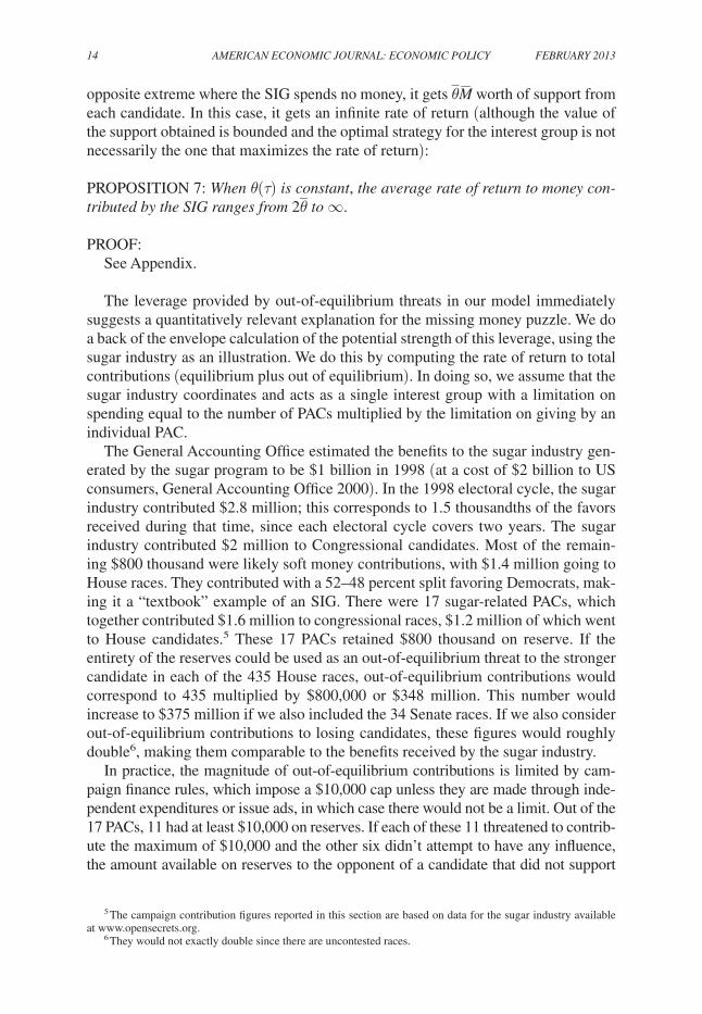
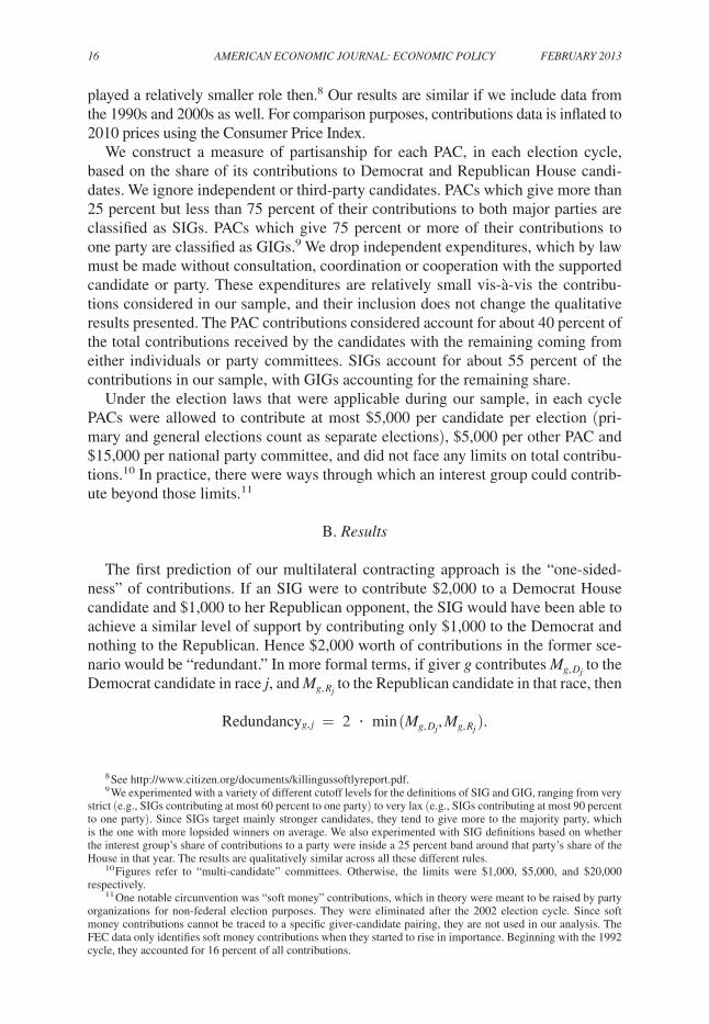
Table 2 confirms our prediction that redundant contributions do not often occur. Thus, while it is very common for PACs to contribute to both Democrat and Republican House candidates, it is extremely rare for them to give to directly oppos-ing candidates. These redundant contributions amount to less than half a percent in lopsided races, but are higher in close races. Standard campaign contribution mod-els predict that SIGs should contribute 50–50 in very close races, implying a 100 percent redundancy of their contributions according to our classification. However, even in the closest of races where the winner has 51 percent or less of the two-party vote, the redundant contributions remain only 7.4 percent of total SIG contributions. This low level of redundancy may result from changes over time in the perceived ex ante strength of the candidates and second order considerations not captured by the model. The table also reports the average share of SIGs contributing to both candidates relative to the total number of contributing SIGs in a race. That figure is also very small with only 5.3 percent in the races where the winner has 51 percent or less of the two-party vote. This finding stands in sharp contrast to the predictions of standard models, such as Grossman and Helpman (1996) and Snyder (1990).
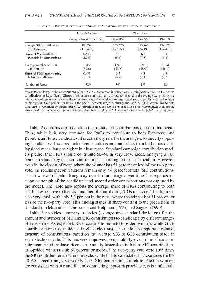
Table 3 provides summary statistics (average and standard deviation) for the amount and number of SIG and GIG contributions to candidates by different ranges of vote share. As expected, SIGs contribute more to lopsided winners while GIGs contribute more to candidates in close elections. The table also reports a relative measure of contributions, based on the average SIG or GIG contribution made in each election cycle. This measure improves comparability over time, since cam-paign contributions have risen substantially faster than inflation. SIG contributions to lopsided winners with 60 percent or more of the two-party vote were 1.65 times the SIG contribution mean in the cycle, while that to candidates in close races (in the 40–60 percent) range were only 1.16. SIG contributions to close election winners are consistent with our multilateral contracting approach provided θ(τ) is sufficiently
Table 2—SIG Contributions and Share of “Redundant” Two-Sided Contributions
Lopsided races Close races
(Winner has 60% or more) [40–60%] [45–55%] [49–51%]
Average SIG contributions 184,796 265,620 275,863 276,973 (2010 dollars) (118,420) (127,650) (124,499) (114,413)Share of “redundant” 0.5% 4.8 6.2 7.4 two-sided contributions (2.2%) (6.6) (7.5) (8.4)
Average number of SIGs 104.2 124.1 126.1 123.4 contributing (57.6) (52.2) (48.9) (41.1)Share of SIGs contributing 0.4% 3.5 4.5 5.3 to both candidates (1.4%) (3.8) (4.2) (4.5)
Number of Races 1,329 367 183 38
notes: Redundancy in the contributions of an SIG in a given race is defined as 2 × min(contributions to Democrat, contributions to Republican). Shares of redundant contributions reported correspond to the average weighted by the total contributions in each race in the respective range. Unweighted averages yield similar results, with redundancy being highest at 8.6 percent for races in the [49–51 percent] range. Similarly, the share of SIGs contributing to both candidates is weighted by the number of contributions in each race in the respective range. Unweighted averages are also very similar to the ones reported, with the share being highest at 5.5 percent for races in the [49–51 percent] range.
18 AmEriCAn ECOnOmiC JOUrnAL: ECOnOmiC POLiCy FEBrUAry 2013
large at τ = 0; contributions to losing candidates are also consistent with our approach if they are the result of ex ante uncertainty. A t-test for differences in means from dif-ferent distributions confirms that lopsided winners receive more SIG contributions than close election candidates. The difference is statistically significant below the 1 percent level for any of the three definitions of closeness used in Table 2. In the case of GIGs, lopsided winners received only 1.23 times the average GIG contribution in the cycle while those in very close races received over twice that average. As in the case of SIGs, the difference in means for lopsided winners and close election candidates is statistically significant below the 1 percent level for any of the definitions of close-ness considered. Previous studies have documented that even though PACs contribute relatively large amounts to winning candidates in lopsided races, they contribute even more to ones involved in close races (e.g., Levitt 1998). The decomposition of PACs between SIGs and GIGs helps to explain that pattern, with SIGs targeting predomi-nantly lopsided winners, GIGs targeting mainly close election candidates and their combination yielding on net more contributions in close elections.
Table 3—SIG and GIG Contributions by Ex Post Vote Share of the Candidate
Lopsided losers Lopsided winners Close election candidates
(Below 40%) (Above 60%) [40–60%] [45–55%] [49–51%]
SIGsAverage contributions 3,232 182,243 132,810*** 137,932*** 138,486*** (2010 dollars) (13,576) (118,262) (137,535) (133,665) (127,451)Average number of 1.9 103.1 64.1*** 65.8*** 64.9*** contributions (7.2) (57.9) (61.7) (58) (51.3)Size of average 1,660 1,768 2,071 2,095 2,134 contribution1 (972) (404) (484) (495) (524)Average contributions 0.03 1.65 1.21*** 1.27*** 1.3*** relative to average in cycle2 (0.12) (1.05) (1.23) (1.21) (1.12)
GIGsAverage contributions 14,108 112,384 161,013*** 180,845*** 202,275*** (2010 dollars) (33,825) (87,497) (135,843) (136,858) (129,276)Average number of 5.4 51.7 52.7*** 58.2*** 63.8*** contributions (10.3) (24.4) (32.5) (30.9) (29.6)Size of average 2,601 2,174 3,058*** 3,110*** 3,168*** contribution1 (1,182) (884) (1,293) (1,293) (1,359)Average contributions 0.16 1.23 1.78*** 2.01*** 2.26*** relative to average in cycle2 (0.38) (0.95) (1.49) (1.51) (1.43)
SIG + GIGsContributions as share 13.5 42.7 33.6*** 33.8*** 36.4*** of candidate’s total receipts (13) (17.6) (16.4) (15.8) (14.3)
Observations 1,050 1,329 734 366 76
notes: Standard deviations reported in parentheses. There are more lopsided winners than losers due to uncontested races.
1 Size of average contribution conditional on a contribution being made. Value reported indicates average for a can-didate in that range of vote share. Average weighted by the number of contributions.
2 Values correspond to the amount received by the candidate from SIGs (GIGs) divided by the average amount received from SIGs (GIGs) by all candidates in that election cycle.
*** Significant at the 1 percent level. ** Significant at the 5 percent level. * Significant at the 10 percent level.
VOL. 5 nO. 1 19Chamon and Kaplan: The ICeberg Theory of CampaIgn ConTrIbuTIons
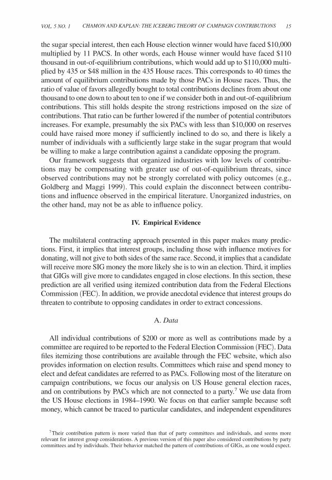
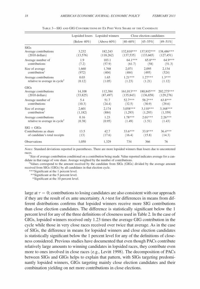
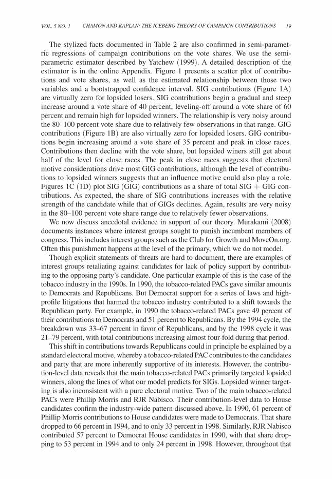
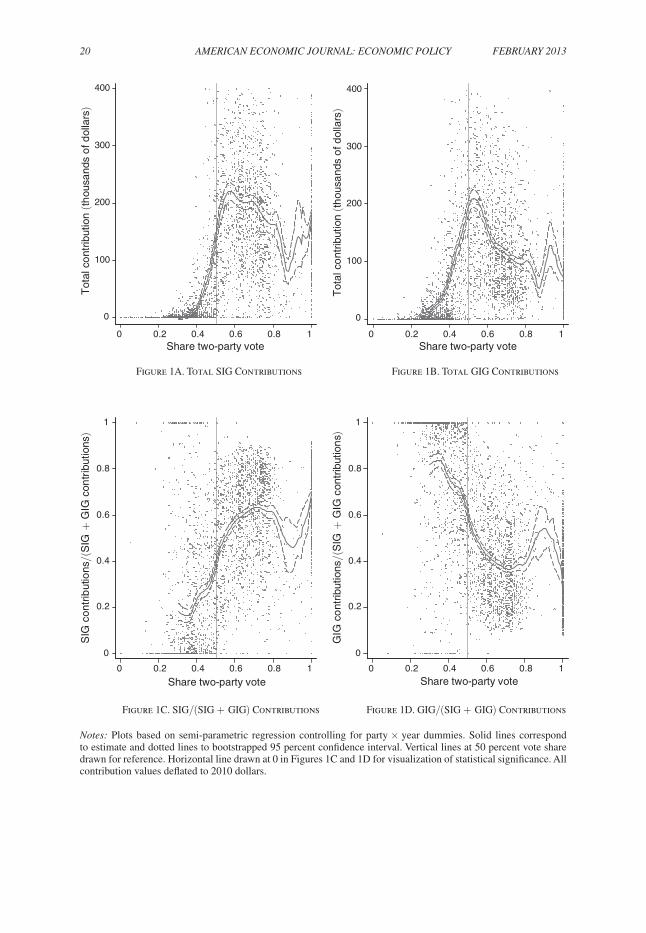
The stylized facts documented in Table 2 are also confirmed in semi-paramet-ric regressions of campaign contributions on the vote shares. We use the semi-parametric estimator described by Yatchew (1999). A detailed description of the estimator is in the online Appendix. Figure 1 presents a scatter plot of contribu-tions and vote shares, as well as the estimated relationship between those two variables and a bootstrapped confidence interval. SIG contributions (Figure 1A) are virtually zero for lopsided losers. SIG contributions begin a gradual and steep increase around a vote share of 40 percent, leveling-off around a vote share of 60 percent and remain high for lopsided winners. The relationship is very noisy around the 80–100 percent vote share due to relatively few observations in that range. GIG contributions (Figure 1B) are also virtually zero for lopsided losers. GIG contribu-tions begin increasing around a vote share of 35 percent and peak in close races. Contributions then decline with the vote share, but lopsided winers still get about half of the level for close races. The peak in close races suggests that electoral motive considerations drive most GIG contributions, although the level of contribu-tions to lopsided winners suggests that an influence motive could also play a role. Figures 1C (1D) plot SIG (GIG) contributions as a share of total SIG + GIG con-tributions. As expected, the share of SIG contributions increases with the relative strength of the candidate while that of GIGs declines. Again, results are very noisy in the 80–100 percent vote share range due to relatively fewer observations.
We now discuss anecdotal evidence in support of our theory. Murakami (2008) documents instances where interest groups sought to punish incumbent members of congress. This includes interest groups such as the Club for Growth and MoveOn.org. Often this punishment happens at the level of the primary, which we do not model.
Though explicit statements of threats are hard to document, there are examples of interest groups retaliating against candidates for lack of policy support by contribut-ing to the opposing party’s candidate. One particular example of this is the case of the tobacco industry in the 1990s. In 1990, the tobacco-related PACs gave similar amounts to Democrats and Republicans. But Democrat support for a series of laws and high-profile litigations that harmed the tobacco industry contributed to a shift towards the Republican party. For example, in 1990 the tobacco-related PACs gave 49 percent of their contributions to Democrats and 51 percent to Republicans. By the 1994 cycle, the breakdown was 33–67 percent in favor of Republicans, and by the 1998 cycle it was 21–79 percent, with total contributions increasing almost four-fold during that period.
This shift in contributions towards Republicans could in principle be explained by a standard electoral motive, whereby a tobacco-related PAC contributes to the candidates and party that are more inherently supportive of its interests. However, the contribu-tion-level data reveals that the main tobacco-related PACs primarily targeted lopsided winners, along the lines of what our model predicts for SIGs. Lopsided winner target-ing is also inconsistent with a pure electoral motive. Two of the main tobacco-related PACs were Phillip Morris and RJR Nabisco. Their contribution-level data to House candidates confirm the industry-wide pattern discussed above. In 1990, 61 percent of Phillip Morris contributions to House candidates were made to Democrats. That share dropped to 66 percent in 1994, and to only 33 percent in 1998. Similarly, RJR Nabisco contributed 57 percent to Democrat House candidates in 1990, with that share drop-ping to 53 percent in 1994 and to only 24 percent in 1998. However, throughout that
20 AmEriCAn ECOnOmiC JOUrnAL: ECOnOmiC POLiCy FEBrUAry 2013
Figure 1C. SIG/(SIG + GIG) Contributions Figure 1D. GIG/(SIG + GIG) Contributions
notes: Plots based on semi-parametric regression controlling for party × year dummies. Solid lines correspond to estimate and dotted lines to bootstrapped 95 percent confidence interval. Vertical lines at 50 percent vote share drawn for reference. Horizontal line drawn at 0 in Figures 1C and 1D for visualization of statistical significance. All contribution values deflated to 2010 dollars.
0
100
200
300
400
0
100
200
300
400T
otal
co
ntrib
utio
n (th
ousa
nds
of d
olla
rs)
Tot
al c
ont
ribut
ion
(thou
sand
s o
f dol
lars
)
0
0.2
0.4
0.6
0.8
1
SIG
con
trib
utio
ns/(
SIG
+ G
IG c
ontr
ibut
ions
)
0 0.2 0.4 0.6 0.8 1
Share two-party vote
GIG
co
ntrib
utio
ns/(
SIG
+ G
IG c
ontr
ibut
ion
s)
0 0.2 0.4 0.6 0.8 1Share two-party vote
0 0.2 0.4 0.6 0.8 1Share two-party vote
0 0.2 0.4 0.6 0.8 1Share two-party vote
0
0.2
0.4
0.6
0.8
1
Figure 1A. Total SIG Contributions Figure 1B. Total GIG Contributions
VOL. 5 nO. 1 21Chamon and Kaplan: The ICeberg Theory of CampaIgn ConTrIbuTIons
time, they continued to target mainly lopsided winners. In 1990, the average share of the two party vote for candidates receiving contributions from these PACs (weighted by contribution size) was 69 percent for both PACs. In 1998, the average share of the two party vote of receiving candidates was 70 percent for Phillip Morris and 67 percent for RJR Nabisco. Thus, even though these tobacco PACs became very closely aligned with the Republican party, the pattern in which they contributed remained distinctively SIG-like, targeting lopsided winners.
Finally, perhaps the SIGs that are in a better position to mobilize the large amounts of resources required to make out of equilibrium threats effective are those related to membership organizations (e.g., AARP or the NRA). Their endorsement or criti-cism of a candidate can lead to a flood of individual contributions. Contributions coordinated by an interest group can add up to substantially more than the campaign contribution limits for a PAC. Unfortunately, it is hard to trace their role in individ-ual contributions even though individual contributions above $200 are recorded by the FEC since we do not have much information on the membership organizations to which individual donors belong.
V. Policy Implications
Our model has interesting implications for campaign finance reform. The Bipartisan Campaign Finance Act of 2002, sometimes referred to as McCain-Feingold, banned soft money contributions though it doubled caps on hard money contributions to candidates and increased limits on allowed contributions to state and national parties. It also indexed future increases to inflation. We now consider the impact of caps on campaign expenditures in our model.
Suppose campaign finance rules lower contribution caps (i.e., further limit contri-butions). The decrease in the cap lowers the SIG’s ability to make out-of-equilibrium threats. The resulting loss in leverage raises the marginal benefit from contributing, which can lead to an increase in equilibrium contributions even though support for the SIG policy declines. To illustrate this counter-intuitive result, we provide neces-sary and sufficient conditions for SIG contributions to go from zero to a positive amount as a result of a tightening of the cap in campaign contributions from an amount
_ m OLD to an amount
_ m nEW >
_ m OLD :
PROPOSITION 8: if θ(τ) is strictly decreasing in τ : ∂ θ _ ∂ τ A , ∂ θ _ ∂ τ B
< 0, then con-tributions from an SiG are zero for a sufficiently high cap on contributions ( _ m OLD ) and positive for a lower (stricter) cap on contributions (
_ m nEW ), if and only if
_ m OLD ≥ θ −1 (min [ 1
_ 1 − 2F(−b) ,
1 _
2F(−b) − 1 ]) > _ m nEW .
PROOF: See Appendix.
The recent Citizens United v. FEC decision of January 2010 made substan-tial changes to legal precedent regarding campaign contributions. A subsequent and related March 2010 decision in FreeSpeech v. FEC now allows unlimited corporate, union, and individual independent expenditures or contributions to
22 AmEriCAn ECOnOmiC JOUrnAL: ECOnOmiC POLiCy FEBrUAry 2013
organizations which make only independent expenditures. According to our the-ory, the impact on special group influence is unambiguously to increase interest group influence. However, effects of increased caps on observed PAC plus inde-pendent expenditures are ambiguous. For large interest groups, the two decisions could lead to a decline in expenditure as they may be able to acheive their goals through out-of-equilibrium threats alone. For smaller interest groups, however, the lifting of the caps should just increase the amount of expenditures they make. On the other hand, PAC contributions were largely unaffected by the rulings. To the degree that independent and PAC expenditures are substitutes, PAC expendi-tures should decline.
VI. Conclusion
In the continuing and unresolved debate on the role of money in politics, the low levels of contributions by special interests have led some to believe that spe-cial interests do not play a large role in the political process. This paper shows how interest groups can sometimes gain support without spending any money, and even the money they do spend only reflects the surface of their influence. In addition to providing an explanation for the “missing money puzzle,” our frame-work also generates a number of stylized facts which are empirically verified. First, contrary to the conventional wisdom (and contrary to many popular models of campaign contributions), we empirically establish that while interest groups often give to both parties, they rarely give to both sides of the same race. Second, we distinguish between special and general interest groups and we predict that general interest groups give to candidates involved in close elections, whereas special interest groups target lopsided winners. These predictions are then veri-fied in the data.
We have limited ourselves to models with a single interest group. Prat and Rustichini (2002) look at models with multiple principals and multiple agents, though without multilateral contracting. Extending the current model to a context with multiple principals would be theoretically interesting, as well as potentially insightful, for the understanding of special interest group behavior.
Certainly our theory suggests that the connection between money spent and the effect of money in politics is not a simple one. Empirical work focusing merely on contributions may merely scratch the surface and underestimate the influence of interest groups. This needs to be kept in mind when analyzing campaign finance rules. Stricter limits on contributions can reduce the effectiveness of out-of-equilibrium threats and cause an increase in equilibrium contributions while limiting the influ-ence of special interests. As shown in this paper, observed contributions can be a very poor guide for the importance of money and the influence of special interests in the political process.
Appendix
PROPOSITION 1: GiG’s never give money to ideologically opposing candidates and give to aligned candidates only in sufficiently close elections.
VOL. 5 nO. 1 23Chamon and Kaplan: The ICeberg Theory of CampaIgn ConTrIbuTIons
PROOF: The GIG’s maximization problem as
max m A , m B
1 − F[− b − m A + m B ] + m GiG − m A − m B
s.t.:
(i) m A , m B ≥ 0, and
(ii) m A + m B ≤ m GiG , and
(iii) m A , m B ≤ _ m .
The first-order condition (FOC) for m B is given by
(4) − f (− b − m A + m B ) − 1 + λ B − λ GiG − λ _ m B = 0,
where λ k is the Kuhn Tucker Lagrange (KTL) multiplier on non-negativity of con-tributions to candidate k (k ∈ {A, B}), λ GiG is the KTL on the GIG’s budget contraint, and λ _ m k is the KTL on the contribution cap to candidate k.
Thus λ B = f (− b + m A − m B ) + 1 + λ GiG + λ _ m B > 0 ⇒ m B * = 0.Conversely, the FOC for m A is given by
(5) f (− b − m A + m B ) − 1 + λ A − λ GiG − λ _ m A = 0,
where λ A is the KTL associated with the non-negativity constraint on contributions to A and λ GiG the one associated with the GIG’s budget constraint. Rearranging, we obtain
max [1 − f (− b − m A + m B ) + λ GiG + λ _ m A , 0] = λ A .
Now, m A * > 0 and m B * = 0 ⇒ λ A = 0 ⇒ f (− b − m A * ) ≥ 1 + λ GiG + λ _ m A ⇒ f (− b − m A * ) ≥ 1. Also, if λ GiG = 0, λ _ m A = 0, then f (− b − m A * ) ≥ 1 ⇒ f (− b − m A * ) ≥1 + λ GiG + λ _ m A ⇒ λ A = 0 ⇒ m A * > 0 and m A * = min [ m GiG ,
_ m ]
> 0 if λ GiG ≠ 0 or λ _ m A ≠ 0 given that m B * = 0. Thus, m A * > 0 ⇔ f (− b − m A * ) ≥ 1 ⇔ ∃z, z′ > 0 such that − b + m A * ∈ (−z, z′ ) ⇔ P(A) ∈ ( _ P ,
_ P ) for some _ P ,
_ P .
PROPOSITION 2: SiGs never give to both sides in the same race.

24 AmEriCAn ECOnOmiC JOUrnAL: ECOnOmiC POLiCy FEBrUAry 2013
PROOF: For notational simplicity, let Δ = − b − (W( τ A ) − W( τ B ) + m A − m B ). We
write the SIG maximization problem as
max m A , m B , τ A , τ B
[1 − F(Δ)] W SiG ( τ A ) + F(Δ) W SiG ( τ B ) + m SiG − m A − m B
+ λ A m A + λ B m B + λ SiG [ m SiG − m A − m B ] + λ _ m A [ _
m − m A ]
+ λ _ m B [ _ m − m B ] + μ A [1 − F(Δ) − 1 + F(− b +
_ m + W( τ B ))]
+ μ B [F(Δ) − F(− b − _ m − W( τ A ))].
We denote the Lagrangian by L. Taking first-order conditions with respect to m A and m B , we obtain
(6) ∂ L _ ∂ m A = f (Δ)[ W SiG ( τ A ) − W SiG ( τ B )] − 1 + λ A − λ SiG − λ _ m A
+ f (Δ)( μ A − μ B ) = 0
(7) ∂ L _ ∂ m B = f (Δ)[ W SiG ( τ B ) − W SiG ( τ A )] − 1 + λ B − λ SiG − λ _ m B
+ f (Δ)( μ B − μ A ) = 0.
Taking first-order conditions with respect to τ A and τ B and dividing by ∂ W( τ k ) _ ∂ τ k
, we obtain
(8) ∂ L _ ∂ τ A = = 0 = [1 − F(Δ)] θ( τ A ) − μ B f (− b −
_ m − W( τ A ))
− f (Δ)[ W SiG ( τ A ) − W SiG ( τ B ) + μ A − μ B ]
(9) ∂ L _ ∂ τ B = = F(Δ)θ( τ B ) − μ A f (− b +
_ m + W( τ B ))
− f (Δ)[ W SiG ( τ B ) − W SiG ( τ A ) + μ B − μ A ] .
Combining (8) with (6) and (9) with (7), we derive
(10) λ A = max [1 + λ SiG + λ _ m A + μ B f (− b − _ m − W( τ A * ))
− [1 − F( Δ * )] θ( τ A * ), 0]
λ B = max [1 + λ SiG + λ _ m B + μ A f (− b + _ m + W( τ B * ))
− F( Δ * )θ( τ B * ), 0],
VOL. 5 nO. 1 25Chamon and Kaplan: The ICeberg Theory of CampaIgn ConTrIbuTIons
where Δ * is Δ with maximized contribution and policy support variables. Adding λ A + λ B , we get
λ A + λ B ≥ + 2 + 2 λ SiG + λ _ m A + λ _ m B + μ A f (− b + _ m + W( τ B * ))
+ μ B f (− b − _ m − W( τ A * )) − [1 − F( Δ * )] θ( τ A * ) − F( Δ * )θ( τ B * ).
Then adding (8) and (9), we obtain
(11) μ A f (− b + _ m + W( τ B * )) + μ B f (− b −
_ m − W( τ A * ))
= [1 − F( Δ * )] θ( τ A * ) + F( Δ * )θ( τ B * ).
Now using (11), we get
λ A + λ B ≥ 2 + 2 λ SiG + λ _ m A + λ _ m B > 0.
This means that at least one of λ A and λ B must be positive and therefore that at least one of m A and m B must be zero. In other words, the SIG will never give to both sides of the same race.
PROPOSITION 3: Candidate outside options always bind.
PROOF: We prove by contradiction. In subpart (i) we show that if a candidate’s outside
option is non-binding, then she will get no money. In (ii) we show that it is never optimal for the SIG to allow the outside options of both candidates to be non-bind-ing. Finally, in (iii) we show that As outside option being non-binding implies B must support the SIG more than A, which contradicts SIG maximization.
(i) μ A = 0 ⇒ m A * = 0: Without loss of generality, assume that the outside option for A is non-binding. Then, μ A = 0 ⇒ μ B f (− b −
_ m − W( τ A * ))
= [1 − F( Δ * )] θ( τ A * ) + F( Δ * )θ( τ B * ) (from equations (11)) ⇒ λ A = 1 + λ SiG + λ _ m A + F( Δ * ) θ( τ A * ) > 0 ⇒ m A * = 0. So, if the outside option for A is non-binding, then A must be getting no money.
(ii) At least one of μ A > 0 or μ B > 0: If both were non-binding, then μ A = μ B = 0. But then equation (11) can not be satisfied. Therefore, at least one out-side option must bind.
(iii) Both μ A > 0 and μ B > 0: Without loss of generality, suppose that the out-side option for candidate A is non-binding. This implies that B’s outside option binds: − W( τ A ) + W( τ B ) − m A + m B = − W( τ A ) −
_ m (from sub-
part (ii)) ⇒ m B − m A = (since m A = 0 from subpart (i)) − _ m − W( τ B )
⇒ m B = − _ m − W( τ B ). Since A’s outside option is non-binding, we also
have − W( τ A ) + W( τ B ) − m A + m B < W( τ B ) + _ m ⇒ − W( τ A ) + m B <
_ m .
26 AmEriCAn ECOnOmiC JOUrnAL: ECOnOmiC POLiCy FEBrUAry 2013
Thus _ m = − m B − W( τ B ) > − W( τ A ) + m B ⇒ W( τ A ) − W( τ B ) > 2 m B ≥ 0
⇒ W( τ A ) > W( τ B ) ⇒ τ B > τ A . This contradicts the solution being a maximum because the SIG can increase τ A , which simultaneously increases the probability that the preferred policy, τ B , is implemented while increasing τ A if candidate A wins:
∂ L SiG _ ∂ τ A
= 0 = [1 − F( Δ * )] θ( τ A * ) − μ B f (− b − _ m − W( τ A * ))
− f ( Δ * )[ W SiG ( τ A * ) − W SiG ( τ B * ) + μ A − μ B ]
= [1 − F( Δ * )] θ( τ A * ) > 0 ⇒ contradiction.
PROPOSITION 4: When outside options are binding, then contributions levels are characterized by
λ A = max [1 + F( Δ * ) θ( τ * ) − [1 − F( Δ * )] θ( τ * ), 0]
λ B = max [1 + [1 − F( Δ * )] θ( τ * ) − F( Δ * )θ( τ * ), 0],
where τ A * = τ B * = τ * = W −1 ( m SiG ).
PROOF: We do this in two parts. First, we show that equilibrium contributions are zero if
and only if politicians support the SIG at the same level. We then use this, in combi-nation with Proposition 3, to characterize contribution levels.
Part I: τ A * = τ B * ⇔ m A * = m B * = 0:(i) m A * = m B * = 0 ⇒ τ A * = τ B * : m A * = m B * = 0 ⇒ −b − W( τ A * ) + W( τ B * ) − m A * + m B * = − b − W( τ A * ) + W( τ B * )
(using the fact that IR constraints bind) = − b − _ m − W( τ A * ) ⇒ W( τ B * ) = −
_ m and
similarly, W( τ A * ) = − _ m ⇒ W( τ A * ) = W( τ B * ) ⇒ τ A * = τ B * .
(ii) τ A * = τ B * ⇒ m A * = m B * = 0: τ A * = τ B * ⇒ −b − W( τ A * ) + W( τ B * ) − m A * + m B * = − b − m A * + m B *
(using the fact that IR constraints bind) = − b − _ m − W( τ A * ) and − b − m A *
+ m B * = − b + _ m + W( τ B * ). Adding the latter two equations, we obtain:
− 2b − W( τ A * ) + W( τ B * ) = − 2b − 2 m A * + 2 m B * (given that τ A * = τ B * and cancel-ling the − 2b) ⇒ m A * = m B * = 0 (by Proposition 2).
Part II: Characterizing contribution levelsFrom Proposition 3 (IR constraints are binding): = f (− b −
_ m − W( τ A * )) f ( Δ * )
= f (− b + _ m + W( τ B * )); thus, we can reduce equation (8) to:
0 = f ( Δ * )[ W SiG ( τ A * ) − W SiG ( τ B * ) + μ A ] − [1 − F( Δ * )] θ( τ A * )
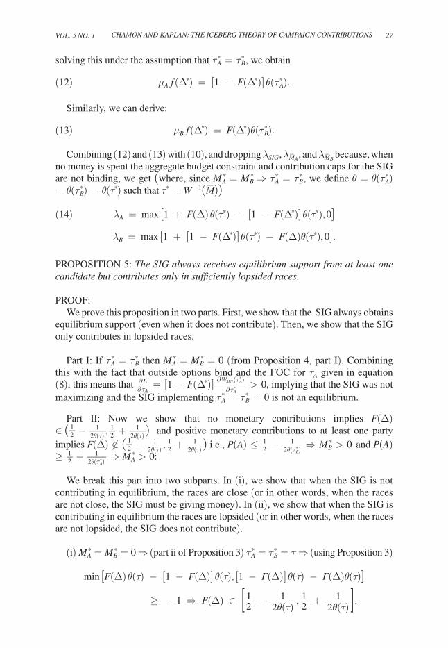
VOL. 5 nO. 1 27Chamon and Kaplan: The ICeberg Theory of CampaIgn ConTrIbuTIons
solving this under the assumption that τ A * = τ B * , we obtain
(12) μ A f ( Δ * ) = [1 − F( Δ * )] θ( τ A * ).
Similarly, we can derive:
(13) μ B f ( Δ * ) = F( Δ * )θ( τ B * ).
Combining (12) and (13) with (10), and dropping λ SiG , λ _ m A , and λ _ m B because, when no money is spent the aggregate budget constraint and contribution caps for the SIG are not binding, we get (where, since m A * = m B * ⇒ τ A * = τ B * , we define θ = θ( τ A * ) = θ( τ B * ) = θ( τ * ) such that τ * = W −1 (
_ m ))
(14) λ A = max [1 + F(Δ) θ( τ * ) − [1 − F( Δ * )] θ( τ * ), 0]
λ B = max [1 + [1 − F( Δ * )] θ( τ * ) − F(Δ)θ( τ * ), 0].
PROPOSITION 5: The SiG always receives equilibrium support from at least one candidate but contributes only in sufficiently lopsided races.
PROOF: We prove this proposition in two parts. First, we show that the SIG always obtains
equilibrium support (even when it does not contribute). Then, we show that the SIG only contributes in lopsided races.
Part I: If τ A * = τ B * then m A * = m B * = 0 (from Proposition 4, part I). Combining this with the fact that outside options bind and the FOC for τ A given in equation (8), this means that ∂ L
_ ∂ τ A = [1 − F( Δ * )] ∂ W SiG ( τ A * )
_ ∂ τ A * > 0, implying that the SIG was not
maximizing and the SIG implementing τ A * = τ B * = 0 is not an equilibrium.
Part II: Now we show that no monetary contributions implies F(Δ)∈ ( 1 _ 2 − 1
_ 2θ(τ) ,
1 _ 2 + 1
_ 2θ(τ) ) and positive monetary contributions to at least one party
implies F(Δ) ∉ ( 1 _ 2 − 1 _
2θ(τ) , 1 _ 2 + 1
_ 2θ(τ) ) i.e., P(A) ≤ 1 _ 2 − 1
_ 2θ( τ B * ) ⇒ m B * > 0 and P(A)
≥ 1 _ 2 + 1 _
2θ( τ A * ) ⇒ m A * > 0:
We break this part into two subparts. In (i), we show that when the SIG is not contributing in equilibrium, the races are close (or in other words, when the races are not close, the SIG must be giving money). In (ii), we show that when the SIG is contributing in equilibrium the races are lopsided (or in other words, when the races are not lopsided, the SIG does not contribute).
(i) m A * = m B * = 0 ⇒ (part ii of Proposition 3) τ A * = τ B * = τ ⇒ (using Proposition 3)
min [F(Δ) θ(τ) − [1 − F(Δ)] θ(τ), [1 − F(Δ)] θ(τ) − F(Δ)θ(τ)]
≥ −1 ⇒ F(Δ) ∈ [ 1 _ 2 − 1 _
2θ(τ) , 1 _ 2 + 1 _
2θ(τ) ].
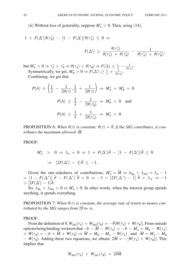
28 AmEriCAn ECOnOmiC JOUrnAL: ECOnOmiC POLiCy FEBrUAry 2013
(ii) Without loss of generality, suppose m A * > 0. Then, using (14),
1 + F( Δ * ) θ( τ B * ) − [1 − F( Δ * )] θ( τ A * ) ≤ 0 ⇒
F( Δ * ) ≤ θ( τ A * ) __ θ( τ A * ) + θ( τ B * ) − 1 __ θ( τ A * ) + θ( τ B * ) ,
but m A * > 0 ⇒ τ A * > τ B * ⇒ θ( τ A ) < θ( τ B ) ⇒ F(Δ) ≤ 1 _ 2 − 1 _
2θ( τ A ) .Symmetrically, we get, m B * > 0 ⇒ F( Δ * ) ≥ 1 _ 2 + 1
_ 2θ( τ B * ) .
Combining, we get that
P(A) ∈ ( 1 _ 2 − 1 _
2θ(τ) , 1 _ 2 + 1 _
2θ(τ) ) ⇒ m A * = m B * = 0
P(A) ≥ 1 _ 2 − 1 _
2θ( τ B * ) ⇒ m B * > 0 and
P(A) ≤ 1 _ 2 + 1 _
2θ( τ A * ) ⇒ m A * > 0.
PROPOSITION 6: When θ(τ) is constant: θ(τ) = _ θ , if the SiG contributes, it con-
tributes the maximum allowed: _ m .
PROOF:
m A * > 0 ⇒ λ A = 0 ⇒ 1 + F( Δ * ) _ θ − [1 − F( Δ * )]
_ θ ≤ 0
⇒ [2F( Δ * ) − 1] _ θ ≤ − 1.
Given the one-sidedness of contributions, m A * = _ m ⇒ λ _ m A + λ SiG = λ A − 1
+ [1 − F( Δ * )] _ θ − F( Δ * )
_ θ > 0 ⇒ −1 > [2F( Δ * ) − 1]
_ θ + λ A ⇒ −1
> [2F( Δ * ) − 1] _ θ .
So, λ _ m A + λ SiG > 0 ⇔ m A * > 0. In other words, when the interest group spends anything, it spends everything.
PROPOSITION 7: When θ(τ) is constant, the average rate of return to money con-tributed by the SiG ranges from 2
_ θ to ∞.
PROOF: From the definition of θ, W SiG ( τ A ) + W SiG ( τ B ) = −
_ θ [W( τ A ) + W( τ B )]. From outside
options being binding, we know that − b − _ m − W( τ A ) = − b − m A + m B − W( τ A )
+ W( τ B ) = − b + _ m + W( τ B ) ⇒
_ m = m B − m A − W( τ A ) and
_ m = m A − m B
− W( τ B ). Adding these two equations, we obtain: 2 _ m = − [W( τ A ) + W( τ B )]. This
implies that
W SiG ( τ A ) + W SiG ( τ B ) = 2 _ θ _ m .

VOL. 5 nO. 1 29Chamon and Kaplan: The ICeberg Theory of CampaIgn ConTrIbuTIons
The average rate of return to money spent is just benefits over expenditures. Without loss of generality, we assume that m A ≥ 0 = m B . Thus the average rate of return is given by
2 _ θ _ m _ m A ,
which ranges from 2 _ θ when m A =
_ m to ∞ when m A = 0.
PROPOSITION 8: if θ(τ) is strictly decreasing in τ : ∂ θ _ ∂ τ A , ∂ θ _ ∂ τ B
< 0, then contribu-tions from an SiG are zero for a sufficiently high cap on contributions (
_ m OLD ) and
positive for a lower (stricter) cap on contributions ( _ m nEW ) if and only if
_ m OLD ≥ θ −1
(min [ 1 _ 1 − 2F(−b) ,
1 _
2F(−b) − 1 ]) > _ m nEW .
PROOF: Main claim: We know that our SIG maximization problem now has two extra
constraints. However, we just want to characterize conditions under which m A = m B = 0 at the old limits ( m A , m B ≤
_ m OLD ) and where either m A > 0 or m B > 0
at the new limits ( m A , m B ≤ _ m nEW <
_ m OLD ). Since we know that our new maxi-
mization problem is the same as the old when the constraints on non-negativity of contribution are binding and since we know that the constraints on non-negativity of contributions are binding if and only if the following equations lead to strictly posi-tive numbers for both λ A and λ B , then we just have to find conditions under which the following equations lead to positive solutions for λ A , λ B under the old cap and not under the new cap:
λ A = 1 + F(− b) θ(τ) − [1 − F(b)] θ(τ)
λ B = 1 + [1 − F(−b)] θ(τ) − F(b)θ(τ),
where F(−b) is the cumulative distribution function giving the probability that can-didate B wins if there are no expenditures ( m A * = m B * = 0) and equal support for the SIG policy (i.e., ⇒ W( τ A ) = W( τ B )).
Now we define θ OLD as the cutoff level of θ(τ) (for W(τ) = − _ m OLD ) such that
all higher levels of θ(τ) will lead to equilibrium contributions given the old cam-paign contribution limits. From λ A ≥ 0, we get 1 ≥ [1 − 2F(−b)] θ OLD or 1
_ 1 − 2F(−b)
≥ θ OLD . Similarly, from λ B ≥ 0, we can derive 1 _
2F(−b) − 1 ≥ θ OLD . Combining these
two inequalities, we get min [ 1 _ 1 − 2F(−b) ,
1 _
2F(−b) − 1 ] ≥ θ OLD . Inverting θ (see subclaim below for a proof that θ −1 depends negatively on
_ m ), we get:
_
m OLD ≥ θ −1 (min [ 1 _ 1 − 2F(−b) ,
1 _
2F(−b) − 1 ]). In order for _ m nEW to not satisfy the
above relations, we must have: θ −1 (min [ 1 _ 1 − 2F(−b) ,
1 _
2F(−b) − 1 ]) > _ m nEW . Thus,
_ m OLD ≥ θ −1 (min [ 1 _
1 − 2F(−b) , 1 _
2F(−b) − 1 ]) >
_ m nEW .
30 AmEriCAn ECOnOmiC JOUrnAL: ECOnOmiC POLiCy FEBrUAry 2013
Subclaim: To complete the proof, we need to show that ∂ θ −1 (
_ m ) _ ∂ τ A
< 0 (where _
m is the statutory limit on campaign contributions). From Proposition 3 (outside options bind), we have − b − W( τ A ) + W( τ B ) − m A + m B = − b −
_ m − W( τ A ), but m A * = m B *
= 0 ⇒ τ A * = τ B * ⇒ − W( τ A * ) + W( τ B * ) = 0. This implies that − b = − b − _
m − W( τ A * ) ⇒ τ A * = − W −1 (
_ m ) ⇒ ∂ τ A *
_ ∂ _
m = − ∂ W −1 (
_ m ) _
∂ _
m > 0 ⇒ ∂ θ( τ A * (
_ m )) _
∂ _
m < 0 ⇒ ∂ θ −1 (
_ m ) _ ∂ τ A
< 0.
REFERENCES
Ansolabehere, Stephen, John M. de Figueiredo, and James M. Snyder, Jr. 2003. “Why Is There So Lit-tle Money in US Politics?” Journal of Economic Perspectives 17 (1): 105–30.
Baron, David P. 1994. “Electoral Competition with Informed and Uninformed Voters.” American Polit-ical Science review 88 (1): 33–47.
Besley, Timothy, and Stephen Coate. 2001. “Lobbying and Welfare in a Representative Democracy.” review of Economic Studies 68 (1): 67–82.
Blundell, Richard, and James Powell. 2000. “Endogeneity in Nonparametric and Semiparametric Regression Models.” Paper presented at Econometric Society World Meeting, Seattle.
Chamon, Marcos, and Ethan Kaplan. 2013. “The Iceberg Theory of Campaign Contributions: Political Threats and Interest Group Behavior: Dataset.” American Economic Journal: Economic Policy. http://dx.doi.org/10.1257/pol.5.1.1.
Dal Bó, Ernesto. 2007. “Bribing Voters.” American Political Science review 51 (4): 789–803.Dixit, Avinash, Gene M. Grossman, and Elhanan Helpman. 1997. “Common Agency and Coordina-
tion: General Theory and Application to Government Policy Making.” Journal of Political Econ-omy 105 (4): 752–69.
Fan, Jianqing. 1992. “Design-Adaptive Nonparametric Regression.” Journal of the American Statisti-cal Association 87 (420): 998–1004.
Fox, Justin, and Laurence Rothenberg. 2011. “Influence without Bribes: A Non-Contracting Model of Campaign Giving and Policymaking.” Political Analysis 19 (3): 325–41.
General Accounting Office. 2000. “Sugar Program: Supporting Sugar Prices has Increased Users’ Costs While Benefitting Producers.” GAO/RCED-00-126, Washington, DC.
Goldberg, Pinelopi Koujianou, and Giovanni Maggi. 1999. “Protection for Sale: An Empirical Investi-gation.” American Economic review 89 (5): 1135–55.
Gopoian, J. David. 1984. “What Makes a PAC Tick? An Analysis of the Allocation Patterns of Eco-nomic Interest Groups.” American Journal of Political Science 28 (2): 259–81.
Grossman, Gene M., and Elhanan Helpman. 1994. “Protection for Sale.” American Economic review 84 (4): 833–50.
Grossman, Gene M., and Elhanan Helpman. 1996. “Electoral Competition and Special Interest Poli-tics.” review of Economic Studies 63 (2): 265–86.
Grossman, Gene M., and Elhanan Helpman. 2001. “Contributions and Elections.” In Special interest Politics, 319–46. Cambridge, MA: MIT Press.
Helpman, Elhanan, and Torsten Persson. 2001. “Lobbying and Legislative Bargaining.” B. E. Journal of Economic Analysis and Policy 1 (1): Article 4.
King, Gary, Bradley Palmquist, Greg Adams, Micah Altman, Kenneth Benoit, Claudine Gay, Jeffrey B. Lewis, Russ Mayer, and Eric Reinhardt. 1997. “The Record of American Democracy, 1984–1990.” Harvard University, Cambridge, MA [producer], Ann Arbor, MI: ICPSR [distributor].
Lessig, Lawrence. 2011. republic, Lost: How money Corrupts Congress–and a Plan to Stop it. New York: Twelve Books.
Levitt, Steven. 1998. “Are PACs Trying to Influence Politicians or Voters?” Economics and Politics 10 (1): 19–36.
Mian, Atif, Amir Sufi, and Francesco Trebbi. 2010. “The Political Economy of the US Mortgage Default Crisis.” American Economic review 100 (5): 1967–98.
Milyo, Jeffrey, David Primo, and Timothy Groseclose. 2000. “Corporate PAC Campaign Contributions in Perspective.” Business and Politics 2 (1): 75–88.
Murakami, Michael. 2008. “Divisive Primaries: Party Organizations, Ideological Groups, and the Bat-tle over Party Purity.” PS: Political Science and Politics 41 (4): 918–23.
VOL. 5 nO. 1 31Chamon and Kaplan: The ICeberg Theory of CampaIgn ConTrIbuTIons
Persson, Torsten, and Guido Tabellini. 2000. “Electoral Competition.” In Political Economics: Explain-ing Economic Policy. Cambridge, MA: MIT Press.
Poole, Keith T., Thomas Romer, and Howard Rosenthal. 1987. “The Revealed Preferences of Political Action Committees.” American Economic review 77 (2): 298–302.
Prat, Andrea, and Aldo Rustichini. 2003. “Games Played through Agents.” Econometrica 71 (4): 989–1026.
Snyder, James M., Jr. 1990. “Campaign Contributions as Investments: The US House of Representa-tives, 1980–1986.” Journal of Political Economy 98 (6): 1195–1227.
Tullock, Gordon. 1972. “The Purchase of Politicians.” Western Economic Journal 10 (3): 354–55.US General Accounting Office. 2000. “Sugar Program: Supporting Sugar Prices Has Increased Users’
Costs While Benefiting Producers.” US General Accounting Office. Washington DC, June.Yatchew, Adonis. 1999. “An Elementary Nonparametric Differencing Test of Equality of Regression
Functions.” Economic Letters 62 (3): 271–78.