The hybrid vertical representation

The vertical coordinate in global models is usually defined using the hybrid vertical

representation. In such a system the vertical layers are defined by their pressure:

pk = Ak + Bk psurf (1)

for k = 1, . . . , N. The coefficients Ak and Bk are constants whose values effectively de-

fine the vertical coordinate, and psurf is the surface pressure.

In the EMAC model the hybrid coefficients are called hyam and hybm for the level mid-

point (i.e. the center of the cell), and hyai and hybi for the level interfaces (i.e. the borders

of the cell). The surface pressure is indicated by aps. In the specific example considered

here, there are 19 vertical layers, i.e. the dimension of hyam and hybm is 19, whereas the

dimension of hyai and hybi is 20 (see Figure 1).

Figure 1: Vertical hybrid levels from the EMAC model in the T42L19 configuration.The plot shows a selected slice at latitude ≃ 52◦S.

1

Exercise 1

• download the sample data file at

http://www.pa.op.dlr.de/̃ MattiaRighi/NCL/LECTURE/NetCDF sample.nc

• open the sample data file NetCDF sample.nc and read the variable O3, represent-

ing ozone concentration in December 2004.

• what are the units of O3? Convert them to ppbv.

• interpolate this variable from hybrid to pressure levels, using 50 equally-spaced

pressure levels ranging from 100 to 1000 hPa (HINT: use the NCL function vinth2p).

• extract the timestep corresponding to 15.12.2004 at 12:00 (HINT: use the NCL

function ut inv calendar and coordinate subscripting).

• compute the zonal average (average of the longitude coordinate).

• plot the result as a pressure-height/latitude plot (HINT: check the examples gallery

on the website).

• customize the plot to get something similar to Figure 2 (HINT: use the wh-bl-gr-ye-re

color map).

2

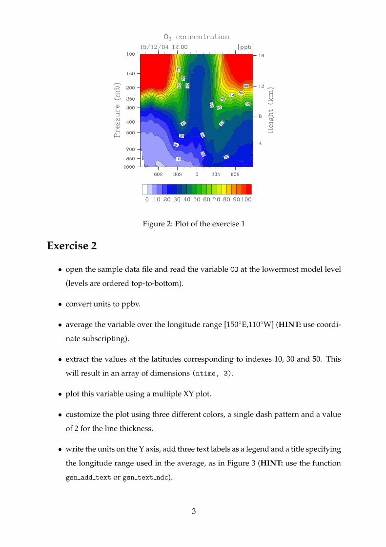
Figure 2: Plot of the exercise 1

Exercise 2

• open the sample data file and read the variable CO at the lowermost model level

(levels are ordered top-to-bottom).

• convert units to ppbv.

• average the variable over the longitude range [150◦E,110◦W] (HINT: use coordi-

nate subscripting).

• extract the values at the latitudes corresponding to indexes 10, 30 and 50. This

will result in an array of dimensions (ntime, 3).

• plot this variable using a multiple XY plot.

• customize the plot using three different colors, a single dash pattern and a value

of 2 for the line thickness.

• write the units on the Y axis, add three text labels as a legend and a title specifying

the longitude range used in the average, as in Figure 3 (HINT: use the function

gsn add text or gsn text ndc).

3

Figure 3: Plot of the exercise 2

The logistic equation

The logistic equation is a simple way to understand the concept of chaos. It was orig-

inally introduced to approximate the evolution of an animal population over time.

Consider a population that has a generation per year. If xn is the number of animals in

the year n, then the number of animal in the following year n + 1 is written as:

xn+1 = r xn (1 − xn), (2)

where r is the growth rate (or fecundity) of the population and the factor (1 − xn)

accounts for the carrying-capacity of the environment. This means that the population

cannot grow beyond a certain limit (for example, because of limited resources).

For a given initial seed value x0, one can show that depending on the value of the

growth rate r the evolution of the population follows different behaviours: fixed (the

population approaches a stable value), periodic (the population oscillates between two

or powers of two fixed values) or chaotic (the population assumes an infinite number of

values in the range [0,1]). This can be visualized with a bifurfaction diagram (Figure 4),

where the values assumed by the population are plotted as a function of r.

4

Figure 4: Bifurcation diagram for the logistic equation (from Wikipedia).

Exercise 3

Apply the logistic equation described in the previous page to obtain a bifurcation dia-

gram similar to the one in Figure 4.

• use x0 = 0.5 as initial seed.

• apply the equation for 300 values of r in the range [1;4].

• for each value of r consider n = 300 iterations.

• skip the first 100 iterations when plotting the population values.

• plot the values of x as a scatter plot (check the corresponding example on the

website), with r on the horizontal axis (HINT: the array to be plotted is a function

of r and of the iteration index (two-dimensional). It needs to be converted to one-

dimensional before plotting).

5

Figure 5: Plot of the exercise 3

6