
The HPCOUNTREG Procedure - SAS
51
SAS/ETS ® 15.2 User’s Guide The HPCOUNTREG Procedure SAS ® Documentation August 17, 2020
Transcript of The HPCOUNTREG Procedure - SAS

SAS/ETS® 15.2User’s GuideThe HPCOUNTREGProcedure
SAS® DocumentationAugust 17, 2020
This document is an individual chapter from SAS/ETS® 15.2 User’s Guide.
The correct bibliographic citation for this manual is as follows: SAS Institute Inc. 2020. SAS/ETS® 15.2 User’s Guide. Cary, NC:SAS Institute Inc.
SAS/ETS® 15.2 User’s Guide
Copyright © 2020, SAS Institute Inc., Cary, NC, USA
All Rights Reserved. Produced in the United States of America.
For a hard-copy book: No part of this publication may be reproduced, stored in a retrieval system, or transmitted, in any form or byany means, electronic, mechanical, photocopying, or otherwise, without the prior written permission of the publisher, SAS InstituteInc.
For a web download or e-book: Your use of this publication shall be governed by the terms established by the vendor at the timeyou acquire this publication.
The scanning, uploading, and distribution of this book via the Internet or any other means without the permission of the publisher isillegal and punishable by law. Please purchase only authorized electronic editions and do not participate in or encourage electronicpiracy of copyrighted materials. Your support of others’ rights is appreciated.
U.S. Government License Rights; Restricted Rights: The Software and its documentation is commercial computer softwaredeveloped at private expense and is provided with RESTRICTED RIGHTS to the United States Government. Use, duplication, ordisclosure of the Software by the United States Government is subject to the license terms of this Agreement pursuant to, asapplicable, FAR 12.212, DFAR 227.7202-1(a), DFAR 227.7202-3(a), and DFAR 227.7202-4, and, to the extent required under U.S.federal law, the minimum restricted rights as set out in FAR 52.227-19 (DEC 2007). If FAR 52.227-19 is applicable, this provisionserves as notice under clause (c) thereof and no other notice is required to be affixed to the Software or documentation. TheGovernment’s rights in Software and documentation shall be only those set forth in this Agreement.
SAS Institute Inc., SAS Campus Drive, Cary, NC 27513-2414
August 2020
SAS® and all other SAS Institute Inc. product or service names are registered trademarks or trademarks of SAS Institute Inc. in theUSA and other countries. ® indicates USA registration.
Other brand and product names are trademarks of their respective companies.
SAS software may be provided with certain third-party software, including but not limited to open-source software, which islicensed under its applicable third-party software license agreement. For license information about third-party software distributedwith SAS software, refer to http://support.sas.com/thirdpartylicenses.
Chapter 19
The HPCOUNTREG Procedure
ContentsOverview: HPCOUNTREG Procedure . . . . . . . . . . . . . . . . . . . . . . . . . . . . . 1022
PROC HPCOUNTREG Features . . . . . . . . . . . . . . . . . . . . . . . . . . . . 1022Getting Started: HPCOUNTREG Procedure . . . . . . . . . . . . . . . . . . . . . . . . . . 1023Syntax: HPCOUNTREG Procedure . . . . . . . . . . . . . . . . . . . . . . . . . . . . . . 1026
Functional Summary . . . . . . . . . . . . . . . . . . . . . . . . . . . . . . . . . . . 1026PROC HPCOUNTREG Statement . . . . . . . . . . . . . . . . . . . . . . . . . . . . 1028BOUNDS Statement . . . . . . . . . . . . . . . . . . . . . . . . . . . . . . . . . . . 1032BY Statement . . . . . . . . . . . . . . . . . . . . . . . . . . . . . . . . . . . . . . 1032CLASS Statement . . . . . . . . . . . . . . . . . . . . . . . . . . . . . . . . . . . . 1033DISPMODEL Statement . . . . . . . . . . . . . . . . . . . . . . . . . . . . . . . . . 1033FREQ Statement . . . . . . . . . . . . . . . . . . . . . . . . . . . . . . . . . . . . . 1034INIT Statement . . . . . . . . . . . . . . . . . . . . . . . . . . . . . . . . . . . . . . 1034MODEL Statement . . . . . . . . . . . . . . . . . . . . . . . . . . . . . . . . . . . . 1034OUTPUT Statement . . . . . . . . . . . . . . . . . . . . . . . . . . . . . . . . . . . 1036PERFORMANCE Statement . . . . . . . . . . . . . . . . . . . . . . . . . . . . . . 1037RESTRICT Statement . . . . . . . . . . . . . . . . . . . . . . . . . . . . . . . . . . 1038TEST Statement . . . . . . . . . . . . . . . . . . . . . . . . . . . . . . . . . . . . . 1039WEIGHT Statement . . . . . . . . . . . . . . . . . . . . . . . . . . . . . . . . . . . 1040ZEROMODEL Statement . . . . . . . . . . . . . . . . . . . . . . . . . . . . . . . . 1040
Details: HPCOUNTREG Procedure . . . . . . . . . . . . . . . . . . . . . . . . . . . . . . 1041Missing Values . . . . . . . . . . . . . . . . . . . . . . . . . . . . . . . . . . . . . . 1041Poisson Regression . . . . . . . . . . . . . . . . . . . . . . . . . . . . . . . . . . . . 1042Conway-Maxwell-Poisson Regression . . . . . . . . . . . . . . . . . . . . . . . . . . 1043Negative Binomial Regression . . . . . . . . . . . . . . . . . . . . . . . . . . . . . . 1047Zero-Inflated Count Regression Overview . . . . . . . . . . . . . . . . . . . . . . . . 1049Zero-Inflated Poisson Regression . . . . . . . . . . . . . . . . . . . . . . . . . . . . 1050Zero-Inflated Conway-Maxwell-Poisson Regression . . . . . . . . . . . . . . . . . . 1051Zero-Inflated Negative Binomial Regression . . . . . . . . . . . . . . . . . . . . . . 1053Parameter Naming Conventions for the RESTRICT, TEST, BOUNDS, and INIT State-
ments . . . . . . . . . . . . . . . . . . . . . . . . . . . . . . . . . . . . . . 1054Computational Resources . . . . . . . . . . . . . . . . . . . . . . . . . . . . . . . . 1057Covariance Matrix Types . . . . . . . . . . . . . . . . . . . . . . . . . . . . . . . . 1058Displayed Output . . . . . . . . . . . . . . . . . . . . . . . . . . . . . . . . . . . . . 1058OUTPUT OUT= Data Set . . . . . . . . . . . . . . . . . . . . . . . . . . . . . . . . 1060OUTEST= Data Set . . . . . . . . . . . . . . . . . . . . . . . . . . . . . . . . . . . 1060ODS Table Names . . . . . . . . . . . . . . . . . . . . . . . . . . . . . . . . . . . . 1060
1022 F Chapter 19: The HPCOUNTREG Procedure
Examples: The HPCOUNTREG Procedure . . . . . . . . . . . . . . . . . . . . . . . . . . 1061Example 19.1: High-Performance Zero-Inflated Poisson Model . . . . . . . . . . . . 1061
References . . . . . . . . . . . . . . . . . . . . . . . . . . . . . . . . . . . . . . . . . . . 1064
Overview: HPCOUNTREG ProcedureThe HPCOUNTREG procedure is a high-performance version of the COUNTREG procedure in SAS/ETSsoftware. Like the COUNTREG procedure, the HPCOUNTREG procedure fits regression models in whichthe dependent variable takes nonnegative integer or count values.
By default, PROC HPCOUNTREG performs computations in multiple threads.
PROC HPCOUNTREG FeaturesThe HPCOUNTREG procedure estimates the parameters of a count regression model by maximum likelihoodtechniques.
The HPCOUNTREG procedure supports the following models for count data:
� Poisson regression
� Conway-Maxwell-Poisson regression
� negative binomial regression with quadratic and linear variance functions (Cameron and Trivedi 1986)
� zero-inflated Poisson (ZIP) model (Lambert 1992)
� zero-inflated Conway-Maxwell-Poisson (ZICMP) model
� zero-inflated negative binomial (ZINB) model
� fixed-effects and random-effects Poisson models for panel data
� fixed-effects and random-effects negative binomial models for panel data
The following list summarizes some basic features of the HPCOUNTREG procedure:
� is multithreaded during all phases of analytic execution
� has model-building syntax that uses CLASS and effect-based MODEL statements familiar fromSAS/ETS analytic procedures
� performs maximum likelihood estimation
� supports multiple link functions
� uses the WEIGHT statement for weighted analysis
Getting Started: HPCOUNTREG Procedure F 1023
� uses the FREQ statement for grouped analysis
� uses the OUTPUT statement to produce a data set that contains predicted probabilities and otherobservationwise statistics
Getting Started: HPCOUNTREG ProcedureExcept for its ability to operate in the multithreaded environment, the HPCOUNTREG procedure is similarto other regression model procedures in the SAS System. For example, the following statements are used toestimate a Poisson regression model:
proc hpcountreg data=one ;model y = x / dist=poisson ;
run;
The response variable y is numeric and has nonnegative integer values.
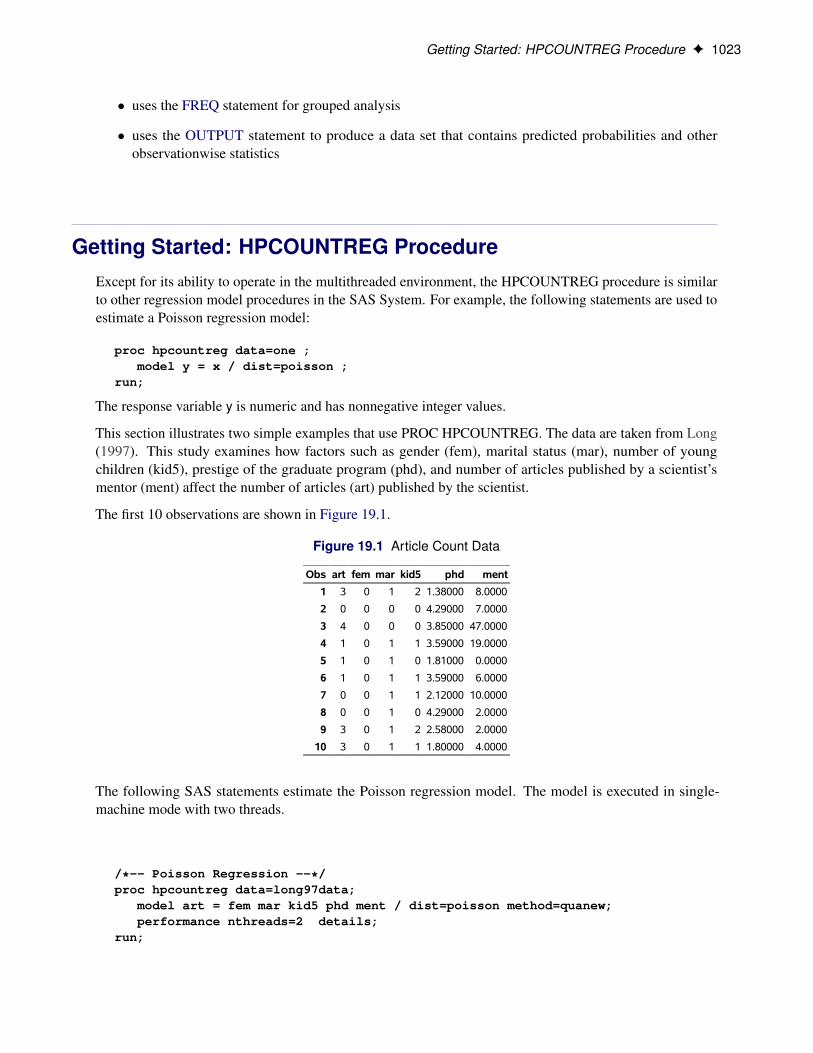
This section illustrates two simple examples that use PROC HPCOUNTREG. The data are taken from Long(1997). This study examines how factors such as gender (fem), marital status (mar), number of youngchildren (kid5), prestige of the graduate program (phd), and number of articles published by a scientist’smentor (ment) affect the number of articles (art) published by the scientist.
The first 10 observations are shown in Figure 19.1.
Figure 19.1 Article Count Data
Obs art fem mar kid5 phd ment
1 3 0 1 2 1.38000 8.0000
2 0 0 0 0 4.29000 7.0000
3 4 0 0 0 3.85000 47.0000
4 1 0 1 1 3.59000 19.0000
5 1 0 1 0 1.81000 0.0000
6 1 0 1 1 3.59000 6.0000
7 0 0 1 1 2.12000 10.0000
8 0 0 1 0 4.29000 2.0000
9 3 0 1 2 2.58000 2.0000
10 3 0 1 1 1.80000 4.0000
The following SAS statements estimate the Poisson regression model. The model is executed in single-machine mode with two threads.
/*-- Poisson Regression --*/proc hpcountreg data=long97data;
model art = fem mar kid5 phd ment / dist=poisson method=quanew;performance nthreads=2 details;
run;
1024 F Chapter 19: The HPCOUNTREG Procedure
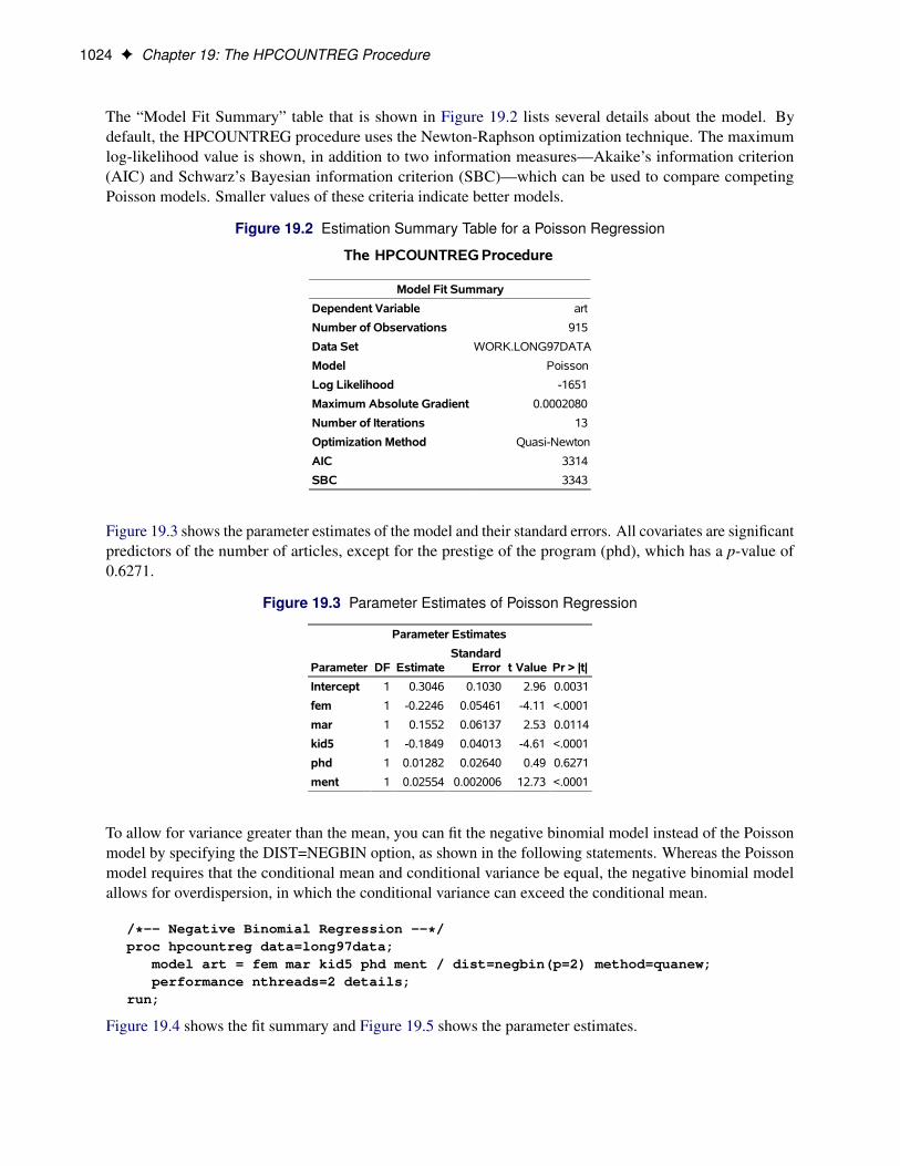
The “Model Fit Summary” table that is shown in Figure 19.2 lists several details about the model. Bydefault, the HPCOUNTREG procedure uses the Newton-Raphson optimization technique. The maximumlog-likelihood value is shown, in addition to two information measures—Akaike’s information criterion(AIC) and Schwarz’s Bayesian information criterion (SBC)—which can be used to compare competingPoisson models. Smaller values of these criteria indicate better models.
Figure 19.2 Estimation Summary Table for a Poisson Regression
The HPCOUNTREG Procedure
Model Fit Summary
Dependent Variable art
Number of Observations 915
Data Set WORK.LONG97DATA
Model Poisson
Log Likelihood -1651
Maximum Absolute Gradient 0.0002080
Number of Iterations 13
Optimization Method Quasi-Newton
AIC 3314
SBC 3343
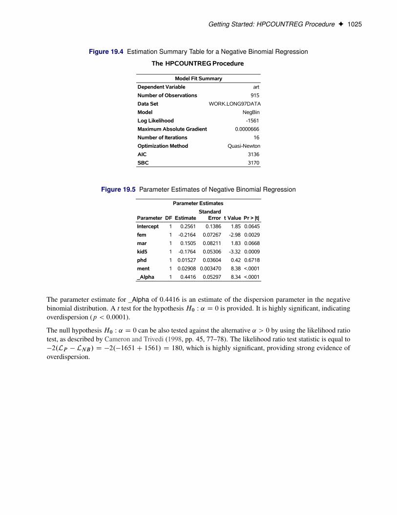
Figure 19.3 shows the parameter estimates of the model and their standard errors. All covariates are significantpredictors of the number of articles, except for the prestige of the program (phd), which has a p-value of0.6271.
Figure 19.3 Parameter Estimates of Poisson Regression
Parameter Estimates
Parameter DF EstimateStandard
Error t Value Pr > |t|
Intercept 1 0.3046 0.1030 2.96 0.0031
fem 1 -0.2246 0.05461 -4.11 <.0001
mar 1 0.1552 0.06137 2.53 0.0114
kid5 1 -0.1849 0.04013 -4.61 <.0001
phd 1 0.01282 0.02640 0.49 0.6271
ment 1 0.02554 0.002006 12.73 <.0001
To allow for variance greater than the mean, you can fit the negative binomial model instead of the Poissonmodel by specifying the DIST=NEGBIN option, as shown in the following statements. Whereas the Poissonmodel requires that the conditional mean and conditional variance be equal, the negative binomial modelallows for overdispersion, in which the conditional variance can exceed the conditional mean.
/*-- Negative Binomial Regression --*/proc hpcountreg data=long97data;
model art = fem mar kid5 phd ment / dist=negbin(p=2) method=quanew;performance nthreads=2 details;
run;
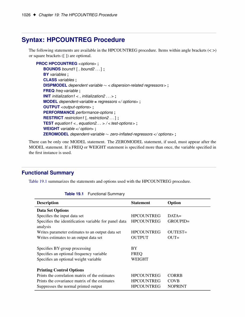
Figure 19.4 shows the fit summary and Figure 19.5 shows the parameter estimates.
Getting Started: HPCOUNTREG Procedure F 1025
Figure 19.4 Estimation Summary Table for a Negative Binomial Regression
The HPCOUNTREG Procedure
Model Fit Summary
Dependent Variable art
Number of Observations 915
Data Set WORK.LONG97DATA
Model NegBin
Log Likelihood -1561
Maximum Absolute Gradient 0.0000666
Number of Iterations 16
Optimization Method Quasi-Newton
AIC 3136
SBC 3170
Figure 19.5 Parameter Estimates of Negative Binomial Regression
Parameter Estimates
Parameter DF EstimateStandard
Error t Value Pr > |t|
Intercept 1 0.2561 0.1386 1.85 0.0645
fem 1 -0.2164 0.07267 -2.98 0.0029
mar 1 0.1505 0.08211 1.83 0.0668
kid5 1 -0.1764 0.05306 -3.32 0.0009
phd 1 0.01527 0.03604 0.42 0.6718
ment 1 0.02908 0.003470 8.38 <.0001
_Alpha 1 0.4416 0.05297 8.34 <.0001
The parameter estimate for _Alpha of 0.4416 is an estimate of the dispersion parameter in the negativebinomial distribution. A t test for the hypothesis H0 W ˛ D 0 is provided. It is highly significant, indicatingoverdispersion (p < 0:0001).
The null hypothesis H0 W ˛ D 0 can be also tested against the alternative ˛ > 0 by using the likelihood ratiotest, as described by Cameron and Trivedi (1998, pp. 45, 77–78). The likelihood ratio test statistic is equal to�2.LP � LNB/ D �2.�1651C 1561/ D 180, which is highly significant, providing strong evidence ofoverdispersion.
1026 F Chapter 19: The HPCOUNTREG Procedure
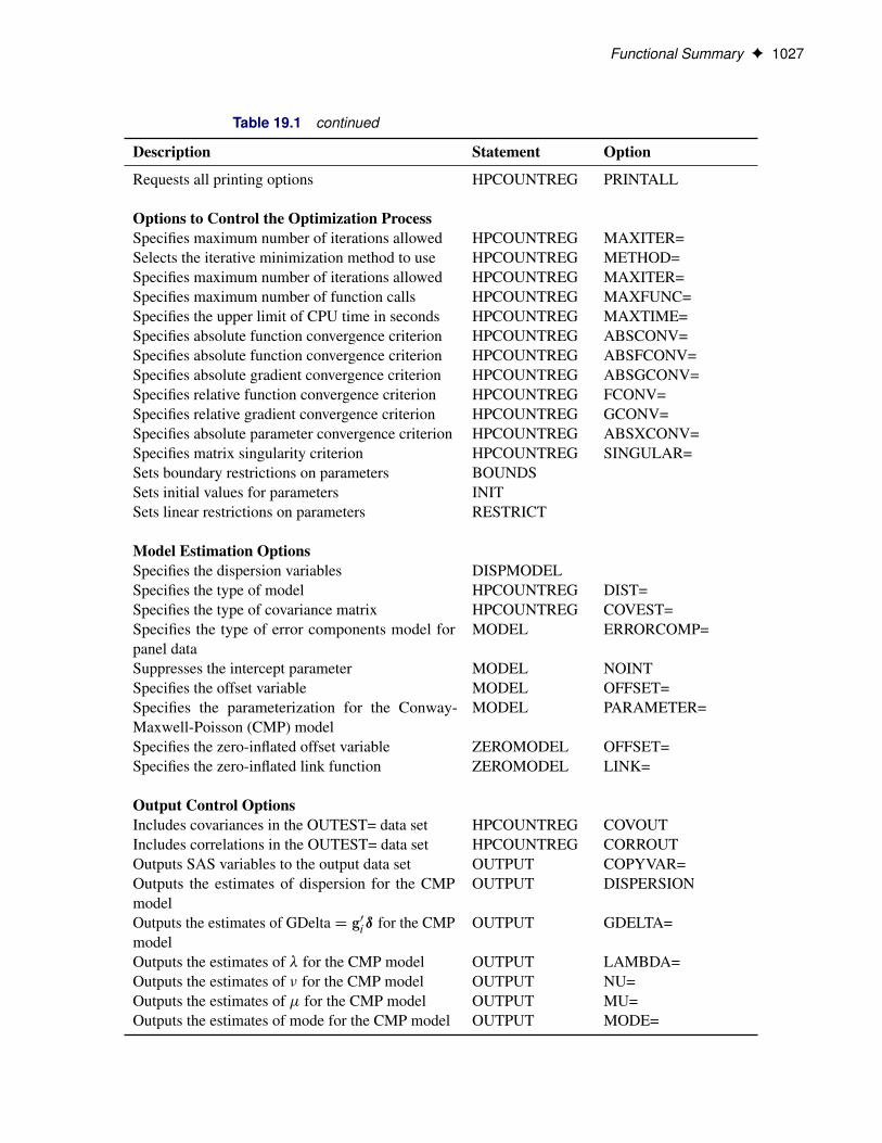
Syntax: HPCOUNTREG ProcedureThe following statements are available in the HPCOUNTREG procedure. Items within angle brackets (< >)or square brackets ([ ]) are optional.
PROC HPCOUNTREG <options> ;BOUNDS bound1 [ , bound2 . . . ] ;BY variables ;CLASS variables ;DISPMODEL dependent variable � < dispersion-related regressors > ;FREQ freq-variable ;INIT initialization1 < , initialization2 . . . > ;MODEL dependent-variable = regressors </ options> ;OUTPUT <output-options> ;PERFORMANCE performance-options ;RESTRICT restriction1 [, restriction2 . . . ] ;TEST equation1 < , equation2. . . > / < test-options > ;WEIGHT variable </ option> ;ZEROMODEL dependent-variable � zero-inflated-regressors </ options> ;
There can be only one MODEL statement. The ZEROMODEL statement, if used, must appear after theMODEL statement. If a FREQ or WEIGHT statement is specified more than once, the variable specified inthe first instance is used.
Functional SummaryTable 19.1 summarizes the statements and options used with the HPCOUNTREG procedure.
Table 19.1 Functional Summary
Description Statement Option
Data Set OptionsSpecifies the input data set HPCOUNTREG DATA=Specifies the identification variable for panel dataanalysis
HPCOUNTREG GROUPID=
Writes parameter estimates to an output data set HPCOUNTREG OUTEST=Writes estimates to an output data set OUTPUT OUT=
Specifies BY-group processing BYSpecifies an optional frequency variable FREQSpecifies an optional weight variable WEIGHT
Printing Control OptionsPrints the correlation matrix of the estimates HPCOUNTREG CORRBPrints the covariance matrix of the estimates HPCOUNTREG COVBSuppresses the normal printed output HPCOUNTREG NOPRINT
Functional Summary F 1027
Table 19.1 continued
Description Statement Option
Requests all printing options HPCOUNTREG PRINTALL
Options to Control the Optimization ProcessSpecifies maximum number of iterations allowed HPCOUNTREG MAXITER=Selects the iterative minimization method to use HPCOUNTREG METHOD=Specifies maximum number of iterations allowed HPCOUNTREG MAXITER=Specifies maximum number of function calls HPCOUNTREG MAXFUNC=Specifies the upper limit of CPU time in seconds HPCOUNTREG MAXTIME=Specifies absolute function convergence criterion HPCOUNTREG ABSCONV=Specifies absolute function convergence criterion HPCOUNTREG ABSFCONV=Specifies absolute gradient convergence criterion HPCOUNTREG ABSGCONV=Specifies relative function convergence criterion HPCOUNTREG FCONV=Specifies relative gradient convergence criterion HPCOUNTREG GCONV=Specifies absolute parameter convergence criterion HPCOUNTREG ABSXCONV=Specifies matrix singularity criterion HPCOUNTREG SINGULAR=Sets boundary restrictions on parameters BOUNDSSets initial values for parameters INITSets linear restrictions on parameters RESTRICT
Model Estimation OptionsSpecifies the dispersion variables DISPMODELSpecifies the type of model HPCOUNTREG DIST=Specifies the type of covariance matrix HPCOUNTREG COVEST=Specifies the type of error components model forpanel data
MODEL ERRORCOMP=
Suppresses the intercept parameter MODEL NOINTSpecifies the offset variable MODEL OFFSET=Specifies the parameterization for the Conway-Maxwell-Poisson (CMP) model
MODEL PARAMETER=
Specifies the zero-inflated offset variable ZEROMODEL OFFSET=Specifies the zero-inflated link function ZEROMODEL LINK=
Output Control OptionsIncludes covariances in the OUTEST= data set HPCOUNTREG COVOUTIncludes correlations in the OUTEST= data set HPCOUNTREG CORROUTOutputs SAS variables to the output data set OUTPUT COPYVAR=Outputs the estimates of dispersion for the CMPmodel
OUTPUT DISPERSION
Outputs the estimates of GDeltaD g0iı for the CMPmodel
OUTPUT GDELTA=
Outputs the estimates of � for the CMP model OUTPUT LAMBDA=Outputs the estimates of � for the CMP model OUTPUT NU=Outputs the estimates of � for the CMP model OUTPUT MU=Outputs the estimates of mode for the CMP model OUTPUT MODE=
1028 F Chapter 19: The HPCOUNTREG Procedure
Table 19.1 continued
Description Statement Option
Outputs the probability that the response variablewill take the current value
OUTPUT PROB=
Outputs probabilities for particular response values OUTPUT PROBCOUNT( )Outputs expected value of response variable OUTPUT PRED=Outputs the estimates of variance for the CMP model OUTPUT VARIANCE=Outputs estimates of XBetaD x0iˇ OUTPUT XBETA=Outputs estimates of ZGammaD z0i OUTPUT ZGAMMA=Outputs probability of a zero value as a result of thezero-generating process
OUTPUT PROBZERO=
Performance OptionsRequests a table that shows a timing breakdown PERFORMANCE DETAILSSpecifies the number of threads to use PERFORMANCE NTHREADS=
PROC HPCOUNTREG StatementPROC HPCOUNTREG <options> ;
The following options can be used in the PROC HPCOUNTREG statement.
Input Data Set Options
DATA=SAS-data-setspecifies the input SAS data set. If the DATA= option is not specified, PROC HPCOUNTREG uses themost recently created SAS data set.
GROUPID=variablespecifies an identification variable when a panel data model is estimated. The identification variable isused as a cross-sectional ID variable.
Output Data Set Options
OUTEST=SAS-data-setwrites the parameter estimates to the specified output data set.
CORROUTwrites the correlation matrix for the parameter estimates to the OUTEST= data set. This option is validonly if the OUTEST= option is specified.
PROC HPCOUNTREG Statement F 1029
COVOUTwrites the covariance matrix for the parameter estimates to the OUTEST= data set. This option is validonly if the OUTEST= option is specified.
Printing Options
You can specify the following options in either the PROC HPCOUNTREG statement or the MODELstatement:
CORRBprints the correlation matrix of the parameter estimates.
COVBprints the covariance matrix of the parameter estimates.
NOPRINTsuppresses all printed output.
PRINTALLrequests all printing options.
Estimation Control Options
You can specify the following options in either the PROC HPCOUNTREG statement or the MODELstatement:
COVEST=HESSIAN | OP | QMLspecifies the type of covariance matrix for the parameter estimates.
The default is COVEST=HESSIAN. You can specify the following values:
HESSIAN specifies the covariance from the Hessian matrix.
OP specifies the covariance from the outer product matrix.
QML specifies the covariance from the outer product and Hessian matrices.
Optimization Control Options
PROC HPCOUNTREG uses the nonlinear optimization (NLO) subsystem to perform nonlinear optimizationtasks. You can specify the following options in either the PROC HPCOUNTREG statement or the MODELstatement.
ABSCONV=r
ABSTOL=rspecifies an absolute function value convergence criterion by which minimization stops whenf .� .k// � r . The default value of r is the negative square root of the largest double-precisionvalue, which serves only as a protection against overflows.
1030 F Chapter 19: The HPCOUNTREG Procedure
ABSFCONV=r
ABSFTOL=rspecifies an absolute function difference convergence criterion by which minimization stops when thefunction value has a small change in successive iterations:
jf .� .k�1// � f .� .k//j � r
The default is 0.
ABSGCONV=r
ABSGTOL=rspecifies an absolute gradient convergence criterion. Optimization stops when the maximum absolutegradient element is small:
maxjjgj .�
.k//j � r
The default is 1E–5.
ABSXCONV=r
ABSXTOL=rspecifies an absolute parameter convergence criterion. Optimization stops when the Euclidean distancebetween successive parameter vectors is small:
k � .k/ � � .k�1/ k2� r
The default is 0.
FCONV=r
FTOL=rspecifies a relative function convergence criterion. Optimization stops when a relative change of thefunction value in successive iterations is small:
jf .� .k// � f .� .k�1//j
jf .� .k�1//j� r
The default value is 2�, where � denotes the machine precision constant, which is the smallest double-precision floating-point number such that 1C � > 1.
GCONV=r
GTOL=rspecifies a relative gradient convergence criterion. For all techniques except CONGRA, optimizationstops when the normalized predicted function reduction is small:
g.� .k//T ŒH .k/��1g.� .k//
jf .� .k//j� r
For the CONGRA technique (where a reliable Hessian estimate H is not available), the followingcriterion is used:
k g.� .k// k22 k s.� .k// k2
k g.� .k// � g.� .k�1// k2 jf .� .k//j� r
The default is 1E–8.
PROC HPCOUNTREG Statement F 1031
MAXFUNC=i
MAXFU=ispecifies the maximum number of function calls in the optimization process. The default is 1,000.
The optimization can terminate only after completing a full iteration. Therefore, the number of functioncalls that are actually performed can exceed the number of calls that are specified by this option.
MAXITER=i
MAXIT=ispecifies the maximum number of iterations in the optimization process. The default is 200.
MAXTIME=rspecifies an upper limit of r seconds of CPU time for the optimization process. The default value isthe largest floating-point double representation of your computer. The time that is specified by thisoption is checked only once at the end of each iteration. Therefore, the actual run time can be muchlonger than r . The actual run time includes the remaining time needed to finish the iteration and thetime needed to generate the output of the results.
METHOD=value
specifies the iterative minimization method to use. The default is METHOD=NEWRAP. You canspecify the following values:
CONGRA specifies the conjugate-gradient method.
DBLDOG specifies the double-dogleg method.
NEWRAP specifies the Newton-Raphson method (this is the default).
NONE specifies that no optimization be performed beyond using the ordinary least squaresmethod to compute the parameter estimates.
NRRIDG specifies the Newton-Raphson Ridge method.
QUANEW specifies the quasi-Newton method.
TRUREG specifies the trust region method.
SINGULAR=rspecifies the general singularity criterion that is applied by the HPCOUNTREG procedure in sweepsand inversions. The default is 1E–8.
1032 F Chapter 19: The HPCOUNTREG Procedure
BOUNDS StatementBOUNDS bound1 [, bound2 . . . ] ;
The BOUNDS statement imposes simple boundary constraints on the parameter estimates. You can specifyany number of BOUNDS statements.
Each bound is composed of parameter names, constants, and inequality operators as follows:
item operator item [ operator item [ operator item . . . ] ]
Each item is a constant, a parameter name, or a list of parameter names. Each operator is <, >, <=, or>=. Parameter names are as shown in the Parameter column of the “Parameter Estimates” table. For moreinformation about how parameters are named in the BOUNDS statement, see the section “Parameter NamingConventions for the RESTRICT, TEST, BOUNDS, and INIT Statements” on page 1054.
You can use both the BOUNDS statement and the RESTRICT statement to impose boundary constraints.However, the BOUNDS statement provides a simpler syntax for specifying these kinds of constraints. Formore information, see the section “RESTRICT Statement” on page 1038.
The following BOUNDS statement illustrates the use of parameter lists to specify boundary constraints.It constrains the estimates of the parameter for z to be negative, the parameters for x1 through x10 to bebetween 0 and 1, and the parameter for x1 in the zero-inflation model to be less than 1.
bounds z < 0,0 < x1-x10 < 1,Inf_x1 < 1;
BY StatementBY variables ;
A BY statement can be used with PROC HPCOUNTREG to obtain separate analyses on observations ingroups defined by the BY variables. When a BY statement appears, the input data set should be sorted inorder of the BY variables.
BY statement processing is not supported when the HPCOUNTREG procedure runs alongside the databaseor alongside the Hadoop Distributed File System (HDFS). These modes are used if the input data are storedin a database or HDFS and the grid host is the appliance that houses the data.
CLASS Statement F 1033
CLASS StatementCLASS variables ;
The CLASS statement names the classification variables to be used in the analysis. Classification variablescan be either character or numeric.
Class levels are determined from the formatted values of the CLASS variables. Thus, you can use formats togroup values into levels. For more information, see the discussion of the FORMAT procedure in Base SASProcedures Guide.
DISPMODEL StatementDISPMODEL dependent-variable � < dispersion-related-regressors > ;
The DISPMODEL statement specifies the dispersion-related-regressors that are used to model dispersion.This statement is ignored unless you specify DIST=CMPOISSON in the MODEL statement. The dependent-variable in the DISPMODEL statement must be the same as the dependent-variable in the MODEL statement.
The dependent-variable that appears in the DISPMODEL statement is directly used to model dispersion.Each of the q variables to the right of the tilde (Ï) has a parameter to be estimated in the regression. Forexample, let g0i be the ith observation’s 1 � .q C 1/ vector of values of the q dispersion explanatory variables(q0 is set to 1 for the intercept term). Then the dispersion is a function of g0iı, where ı is the .qC1/�1 vectorof parameters to be estimated, the dispersion model intercept is ı0, and the coefficients for the q dispersioncovariates are ı1; : : : ; ıq . If you specify DISP=CMPOISSON in the MODEL statement but do not include aDISPMODEL statement, then only the intercept term ı0 is estimated. The “Parameter Estimates” table inthe displayed output shows the estimates for the dispersion intercept and dispersion explanatory variables;they are labeled with the prefix “Disp_”. For example, the dispersion intercept is labeled “Disp_Intercept”.If you specify Age (a variable in your data set) as a dispersion explanatory variable, then the “ParameterEstimates” table labels the corresponding parameter estimate “Disp_Age”. The following statements fit aConway-Maxwell-Poisson model by using the regressors SEX, ILLNESS, and INCOME and by using AGEas a dispersion-related regressor:
proc hpcountreg data=docvisit;model doctorvisits=sex illness income / dist=cmpoisson;dispmodel doctorvisits ~ age;
run;
1034 F Chapter 19: The HPCOUNTREG Procedure
FREQ StatementFREQ freq-variable ;
The FREQ statement identifies a variable (freq-variable) that contains the frequency of occurrence of eachobservation. PROC HPCOUNTREG treats each observation as if it appears n times, where n is the valueof freq-variable for the observation. If the value for the observation is not an integer, it is truncated to aninteger. If the value is less than 1 or missing, the observation is not used in the model fitting. When the FREQstatement is not specified, each observation is assigned a frequency of 1.
INIT StatementINIT initialization1 < , initialization2 . . . > ;
The INIT statement sets initial values for parameters in the optimization.
Each initialization is written as a parameter or parameter list, followed by an optional equal sign (=), followedby a number:
parameter <=> number
Parameter names are as shown in the Parameter column of the “Parameter Estimates” table. For moreinformation about how parameters are named in the INIT statement, see the section “Parameter NamingConventions for the RESTRICT, TEST, BOUNDS, and INIT Statements” on page 1054.
MODEL StatementMODEL dependent-variable = regressors </ options> ;
The MODEL statement specifies the dependent variable and independent regressor variables for the regressionmodel. The dependent count variable should take only nonnegative integer values from the input dataset. PROC HPCOUNTREG rounds any positive noninteger count value to the nearest integer. PROCHPCOUNTREG discards any observation that has a negative count.
Only one MODEL statement can be specified. You can specify the following options in the MODELstatement after a slash (/):
DIST=valuespecifies a type of model to be analyzed. You can specify the following values:
POISSON | P specifies the Poisson regression model.
CMPOISSON | C | CMP specifies a Conway-Maxwell-Poisson regression model.
NEGBIN(P=1) specifies the negative binomial regression model that uses a linear variancefunction.
NEGBIN(P=2) | NEGBIN specifies the negative binomial regression model that uses a quadraticvariance function.
ZIPOISSON | ZIP specifies zero-inflated Poisson regression.
MODEL Statement F 1035
ZICMPOISSON | ZICMP specifies a zero-inflated Conway-Maxwell-Poisson regression. The ZERO-MODEL statement must be specified when this model type is specified.
ZINEGBIN | ZINB specifies zero-inflated negative binomial regression.
You can also specify the DIST option in the HPCOUNTREG statement.
ERRORCOMP=FIXED | RANDOMspecifies a type of conditional panel model to be analyzed. You can specify the following model types:
FIXED specifies a fixed-effect error component regression model.
RANDOM specifies a random-effect error component regression model.
NOINTsuppresses the intercept parameter.
OFFSET=offset-variablespecifies a variable in the input data set to be used as an offset variable. The offset-variable is used toallow the observational units to vary across observations. For example, when the number of shippingaccidents could be measured across different time periods or the number of students who participate inan activity could be reported across different class sizes, the observational units need to be adjustedto a common denominator by using the offset variable. The offset variable appears as a covariate inthe model with its parameter restricted to 1. The offset variable cannot be the response variable, thezero-inflation offset variable (if any), or any of the explanatory variables. The “Model Fit Summary”table gives the name of the data set variable that is used as the offset variable; it is labeled “Offset.”
PARAMETER=MU | LAMBDAspecifies the parameterization for the Conway-Maxwell-Poisson model. The following parameteriza-tions are supported:
LAMBDA estimates the original Conway-Maxwell-Poisson model (Shmueli et al. 2005).
MU reparameterizes � as documented by Guikema and Coffelt (2008), where � D �1=�
and the integral part of � represents the mode, which can be considered a measureof central tendency (mean).
By default, PARAMETER=MU.
Printing Options
You can specify the following options in either the PROC HPCOUNTREG statement or the MODELstatement:
CORRBprints the correlation matrix of the parameter estimates.
1036 F Chapter 19: The HPCOUNTREG Procedure
COVBprints the covariance matrix of the parameter estimates.
NOPRINTsuppresses all printed output.
PRINTALLrequests all printing options.
OUTPUT StatementOUTPUT < output-options > ;
The OUTPUT statement creates a new SAS data set that includes variables created by the output-options.These variables include the estimates of x0iˇ, the expected value of the response variable, and the probabilityof the response variable taking on the current value. Furthermore, if a zero-inflated model was fit, you canrequest that the output data set contain the estimates of z0i and the probability that the response is zero as aresult of the zero-generating process. For the Conway-Maxwell-Poisson model, the estimates of g0iı, �, �,�, mode, variance, and dispersion are also available. Except for the probability of the current value, thesestatistics can be computed for all observations in which the regressors are not missing, even if the response ismissing. By adding observations that have missing response values to the input data set, you can computethese statistics for new observations or for settings of the regressors that are not present in the data withoutaffecting the model fit.
You can specify only one OUTPUT statement. You can specify the following output-options:
OUT=SAS-data-setnames the output data set
COPYVAR=SAS-variable-names
COPYVARS=SAS-variable-namesadds SAS variables to the output data set.
XBETA=namenames the variable to contain estimates of x0iˇ.
PRED=name
MEAN=namenames the variable to contain the predicted value of the response variable.
PROB=namenames the variable to contain the probability that the response variable will take the actual value,Pr(Y D yi ).
PROBCOUNT(value1 < value2 . . . >)outputs the probability that the response variable will take particular values. Each value should be anonnegative integer. If you specify a noninteger, it is rounded to the nearest integer. The value canalso be a list of the form X TO Y BY Z. For example, PROBCOUNT(0 1 2 TO 10 BY 2 15) requestspredicted probabilities for counts 0, 1, 2, 4, 5, 6, 8, 10, and 15. This option is not available for thefixed-effects and random-effects panel models.
PERFORMANCE Statement F 1037
ZGAMMA=namenames the variable to contain estimates of z0i .
PROBZERO=namenames the variable to contain the value of 'i , which is the probability that the response variable willtake the value of 0 as a result of the zero-generating process. This variable is written to the output fileonly if the model is zero-inflated.
GDELTA=nameassigns a name to the variable that contains estimates of g0iı for the Conway-Maxwell-Poissondistribution.
LAMBDA=nameassigns a name to the variable that contains the estimate of � for the Conway-Maxwell-Poissondistribution.
NU=nameassigns a name to the variable that contains the estimate of � for the Conway-Maxwell-Poissondistribution.
MU=nameassigns a name to the variable that contains the estimate of � for the Conway-Maxwell-Poissondistribution.
MODE=nameassigns a name to the variable that contains the integral part of � (mode) for the Conway-Maxwell-Poisson distribution.
VARIANCE=nameassigns a name to the variable that contains the estimate of variance for the Conway-Maxwell-Poissondistribution.
DISPERSION=nameassigns a name to the variable that contains the value of dispersion for the Conway-Maxwell-Poissondistribution.
PERFORMANCE StatementPERFORMANCE < performance-options > ;
The PERFORMANCE statement specifies options to control the multithreaded computing environment andrequests detailed results about the performance characteristics of the HPCOUNTREG procedure. The mostcommonly used performance-options in the PERFORMANCE statement are as follows:
DETAILSrequests a table that shows a timing breakdown of the procedure steps.
1038 F Chapter 19: The HPCOUNTREG Procedure
NTHREADS=nspecifies the number of threads for analytic computations and overrides the SAS system optionTHREADS | NOTHREADS. If you do not specify the NTHREADS= option, PROC HPCOUNTREGcreates one thread per CPU for the analytic computations.
The PERFORMANCE statement is documented further in the section “PERFORMANCE Statement” (Chap-ter 20, SAS/STAT User’s Guide).
RESTRICT StatementRESTRICT restriction1 [, restriction2 . . . ] ;
The RESTRICT statement imposes linear restrictions on the parameter estimates. You can specify anynumber of RESTRICT statements.
Each restriction is written as an expression, followed by an equality operator (=) or an inequality operator (<,>, <=, >=) and then by a second expression, as follows:
expression operator expression
The operator can be =, <, >, <=, or >=.
Restriction expressions can be composed of parameter names, constants, and the following operators: times(�), plus (C), and minus (�). Parameter names are as shown in the Effect column of the “Parameter Estimates”table. The restriction expressions must be a linear function of the variables.
Parameter names are as shown in the Parameter column of the “Parameter Estimates” table. For moreinformation about how parameters are named in the RESTRICT statement, see the section “ParameterNaming Conventions for the RESTRICT, TEST, BOUNDS, and INIT Statements” on page 1054.
Lagrange multipliers are reported in the “Parameter Estimates” table for all the active linear constraints. Theyare identified by the names Restrict1, Restrict2, and so on. The probabilities of these Lagrange multipliersare computed using a beta distribution (LaMotte 1994). Nonactive (nonbinding) restrictions have no effecton the estimation results and are not noted in the output.
The following RESTRICT statement constrains the negative binomial dispersion parameter ˛ to 1, whichrestricts the conditional variance to be �C �2:
restrict _Alpha = 1;
TEST Statement F 1039
TEST Statement<label:> TEST <'string'> equation1 < , equation2. . . > / < test-options > ;
The TEST statement performs Wald, Lagrange multiplier, and likelihood ratio tests of linear hypothesesabout the regression parameters that are specified in the preceding MODEL statement.
You can add a label (which is printed in the output) to a TEST statement in two ways: add an unquotedlabel followed by a colon before the TEST keyword, or add a quoted string after the TEST keyword. Theunquoted label cannot contain any spaces. If you include both an unquoted label and a quoted string, PROCHPCOUNTREG uses the unquoted label . If you specify neither an unquoted label nor a quoted string, PROCHPCOUNTREG automatically labels the tests.
Each equation specifies a linear hypothesis to be tested and consists of regression parameter names andrelational operators. The regression parameter names are as shown in the Parameter column of the “ParameterEstimates” table. For more information about how parameters are named in the TEST statement, see thesection “Parameter Naming Conventions for the RESTRICT, TEST, BOUNDS, and INIT Statements” onpage 1054. Only linear equality restrictions and tests are permitted in PROC COUNTREG. Test equationscan consist only of algebraic operations that involve the addition symbol (+), subtraction symbol (-), andmultiplication symbol (*).
All hypotheses in one TEST statement are tested jointly.
You can specify the following test-options after a slash (/):
ALLrequests Wald, Lagrange multiplier, and likelihood ratio tests.
LMrequests the Lagrange multiplier test.
LRrequests the likelihood ratio test.
WALDrequests the Wald test.
By default, the Wald test is performed.
The following illustrates the use of the TEST statement:
proc hpcountreg;model y = x1 x2 x3;test x1 = 0, x2 * .5 + 2 * x3 = 0;test _int: test intercept = 0, x3 = 0;
run;
The first test investigates the joint hypothesis that
ˇ1 D 0
and
0:5ˇ2 C 2ˇ3 D 0
1040 F Chapter 19: The HPCOUNTREG Procedure
Only linear equality restrictions and tests are permitted in PROC HPCOUNTREG. Tests expressions canconsist only of algebraic operations that involve the addition symbol (+), subtraction symbol (-), andmultiplication symbol (*).
WEIGHT StatementWEIGHT variable < / option > ;
The WEIGHT statement specifies a variable to supply weighting values to use for each observation inestimating parameters. The log likelihood for each observation is multiplied by the corresponding weightvariable value.
If the weight of an observation is nonpositive, that observation is not used in the estimation.
The following option can be added to the WEIGHT statement after a slash (/):
NONORMALIZEdoes not normalize the weights. (By default, the weights are normalized so that they add up to theactual sample size. The weights wi are normalized by multiplying them by nPn
iD1wi, where n is the
sample size.) If the weights are required to be used as they are, then specify the NONORMALIZEoption.
ZEROMODEL StatementZEROMODEL dependent-variable � zero-inflated-regressors < / options > ;
The ZEROMODEL statement is required if either ZIP or ZINB is specified in the DIST= option in theMODEL statement. If ZIP or ZINB is specified, then the ZEROMODEL statement must follow the MODELstatement. The dependent variable in the ZEROMODEL statement must be the same as the dependentvariable in the MODEL statement.
The zero-inflated (ZI) regressors appear in the equation that determines the probability ('i ) of a zero count.Each of these q variables has a parameter to be estimated in the regression. For example, let z0i be the ithobservation’s 1 � .q C 1/ vector of values of the q ZI explanatory variables (w0 is set to 1 for the interceptterm). Then 'i is a function of z0i , where is the .q C 1/ � 1 vector of parameters to be estimated. (Thezero-inflated intercept is 0; the coefficients for the q zero-inflated covariates are 1; : : : ; q .) If q is equal to0 (no ZI explanatory variables are provided), then only the intercept term 0 is estimated. The “ParameterEstimates” table in the displayed output shows the estimates for the ZI intercept and ZI explanatory variables;they are labeled with the prefix “Inf_”. For example, the ZI intercept is labeled “Inf_intercept”. If you specifyAge (a variable in your data set) as a ZI explanatory variable, then the “Parameter Estimates” table labels thecorresponding parameter estimate “Inf_Age”.
You can specify the following options in the ZEROMODEL statement after a slash (/):
Details: HPCOUNTREG Procedure F 1041
LINK=LOGISTIC | NORMALspecifies the distribution function used to compute probability of zeros. The supported distributionfunctions are as follows:
LOGISTIC specifies logistic distribution.
NORMAL specifies standard normal distribution.
If this option is omitted, then the default ZI link function is logistic.
OFFSET=zero-inflated-offset-variablespecifies a variable in the input data set to be used as a zero-inflated (ZI) offset variable. The ZIoffset variable zero-inflated-offset-variable is included as a term, with coefficient restricted to 1, inthe equation that determines the probability ('i ) of a zero count and represents an adjustment to acommon observational unit. The ZI offset variable cannot be the response variable, the offset variable(if any), or any of the explanatory variables. The name of the data set variable that is used as the ZIoffset variable is displayed in the “Model Fit Summary” table, where it is labeled as “Inf_offset”.
Details: HPCOUNTREG Procedure
Missing ValuesAny observations in the input data set that have a missing value for one or more of the regressors are ignoredby PROC HPCOUNTREG and not used in the model fit. PROC HPCOUNTREG rounds any positivenoninteger count values to the nearest integer and ignores any observations that have a negative count.
If the input data set contains any observations that have missing response values but nonmissing regressors,PROC HPCOUNTREG can compute several statistics and store them in an output data set by using theOUTPUT statement. For example, you can request that the output data set contain the estimates of x0iˇ, theexpected value of the response variable, and the probability that the response variable will take the currentvalue. Furthermore, if a zero-inflated model was fit, you can request that the output data set contain theestimates of z0i , and the probability that the response is 0 as a result of the zero-generating process. Notethat the presence of such observations (that have missing response values) does not affect the model fit.
1042 F Chapter 19: The HPCOUNTREG Procedure
Poisson RegressionThe most widely used model for count data analysis is Poisson regression. Poisson regression assumes thatyi , given the vector of covariates xi , is independently Poisson distributed with
P.Yi D yi jxi / De��i�
yi
i
yi Š; yi D 0; 1; 2; : : :
and the mean parameter—that is, the mean number of events per period—is given by
�i D exp.x0iˇ/
where ˇ is a .k C 1/ � 1 parameter vector. (The intercept is ˇ0; the coefficients for the k regressors areˇ1; : : : ; ˇk .) Taking the exponential of x0iˇ ensures that the mean parameter �i is nonnegative. It can beshown that the conditional mean is given by
E.yi jxi / D �i D exp.x0iˇ/
Note that the conditional variance of the count random variable is equal to the conditional mean in the Poissonregression model:
V.yi jxi / D E.yi jxi / D �i
The equality of the conditional mean and variance of yi is known as equidispersion.
The standard estimator for the Poisson model is the maximum likelihood estimator (MLE). Because theobservations are independent, the log-likelihood function is written as
L DNXiD1
.��i C yi ln�i � lnyi Š/ DNXiD1
.�ex0iˇC yix0iˇ � lnyi Š/
For more information about the Poisson regression model, see the section “Poisson Regression” on page 607.
The Poisson model has been criticized for its restrictive property that the conditional variance equals theconditional mean. Real-life data are often characterized by overdispersion—that is, the variance exceeds themean. Allowing for overdispersion can improve model predictions because the Poisson restriction of equalmean and variance results in the underprediction of zeros when overdispersion exists. The most commonlyused model that accounts for overdispersion is the negative binomial model. Conway-Maxwell-Poissonregression enables you to model both overdispersion and underdispersion.
Conway-Maxwell-Poisson Regression F 1043
Conway-Maxwell-Poisson RegressionThe Conway-Maxwell-Poisson (CMP) distribution is a generalization of the Poisson distribution that enablesyou to model both underdispersed and overdispersed data. It was originally proposed by Conway andMaxwell (1962), but its implementation to model under- and overdispersed count data is attributed to Shmueliet al. (2005).
Recall that yi , given the vector of covariates xi , is independently Poisson-distributed as
P.Yi D yi jxi / De��i�
yi
i
yi Š; yi D 0; 1; 2; : : :
The Conway-Maxwell-Poisson distribution is defined as
P.Yi D yi jxi ; zi / D1
Z.�i ; �i /
�yi
i
.yi Š/�i; yi D 0; 1; 2; : : :
where the normalization factor is
Z.�i ; �i / D
1XnD0
�ni.nŠ/�i
and
�i D exp.x0iˇ/
�i D � exp.g0iı/
The ˇ vector is a .k C 1/ � 1 parameter vector. (The intercept is ˇ0, and the coefficients for the k regressorsare ˇ1; : : : ; ˇk .) The ı vector is an .mC 1/ � 1 parameter vector. (The intercept is represented by ı0, andthe coefficients for the m regressors are ı1; : : : ; ık .) The covariates are represented by xi and gi vectors.
One of the restrictive properties of the Poisson model is that the conditional mean and variance must beequal:
E.yi jxi / D V.yi jxi / D �i D exp.x0iˇ/
The CMP distribution overcomes this restriction by defining an additional parameter, �, which governs therate of decay of successive ratios of probabilities such that
P.Yi D yi � 1/=P.Yi D yi / D.yi /
�i
�i
The introduction of the additional parameter, �, allows for flexibility in modeling the tail behavior of thedistribution. If � D 1, the ratio is equal to the rate of decay of the Poisson distribution. If � < 1, the rateof decay decreases, enabling you to model processes that have longer tails than the Poisson distribution(overdispersed data). If � > 1, the rate of decay increases in a nonlinear fashion, thus shortening the tail ofthe distribution (underdispersed data).
There are several special cases of the Conway-Maxwell-Poisson distribution. If � < 1 and � ! 1, theConway-Maxwell-Poisson results in the Bernoulli distribution. In this case, the data can take only the values0 and 1, which represents an extreme underdispersion. If � D 1, the Poisson distribution is recovered with
1044 F Chapter 19: The HPCOUNTREG Procedure
its equidispersion property. When � D 0 and � < 1, the normalization factor is convergent and forms ageometric series,
Z.�i ; 0/ D1
1 � �i
and the probability density function becomes
P.Y D yi I�i ; �i D 0/ D .1 � �i /�yi
i
The geometric distribution represents a case of severe overdispersion.
Mean, Variance, and Dispersion for the Conway-Maxwell-Poisson Model
The mean and the variance of the Conway-Maxwell-Poisson distribution are defined as
EŒY � D@ lnZ@ ln�
V ŒY � D@2 lnZ@2 ln�
The Conway-Maxwell-Poisson distribution does not have closed-form expressions for its moments in termsof its parameters � and �. However, the moments can be approximated. Shmueli et al. (2005) use asymptoticexpressions for Z to derive E.Y / and V.Y / as
EŒY � � �1=� C1
2��1
2
V ŒY � �1
��1=�
In the Conway-Maxwell-Poisson model, the summation of infinite series is evaluated using a logarithmicexpansion. The mean and variance are calculated as follows for the Shmueli et al. (2005) model:
E.Y / D1
Z.�; �/
1XjD0
j�j
.j Š/�
V.Y / D1
Z.�; �/
1XjD0
j 2�j
.j Š/��E.Y /2
The dispersion is defined as
D.Y / DV.Y /
E.Y /
Conway-Maxwell-Poisson Regression F 1045
Likelihood Function for the Conway-Maxwell-Poisson Model
The likelihood for a set of n independently and identically distributed variables y1; y2; : : : ; yn is written as
L.y1; y2; : : : ; ynj�; �/ D
QniD1�
yi
.QniD1 yi Š/
�Z.�; �/�n
D �Pn
iD1 yi exp .��nXiD1
ln.yi Š//Z.�; �/�n
D �S1 exp .��S2/Z.�; �/�n
where S1 and S2 are sufficient statistics for y1; y2; : : : ; yn. You can see from the preceding equation that theConway-Maxwell-Poisson distribution is a member of the exponential family. The log-likelihood functioncan be written as
L D �n ln.Z.�; �//CnXiD1
.yi ln.�/ � � ln.yi Š//
The gradients can be written as
Lˇ D NXkD1
yk � n�Z.�; �/�Z.�; �/
!x
Lı D NXkD1
ln.ykŠ/ � nZ.�; �/�Z.�; �/
!�z
Conway-Maxwell-Poisson Regression: Guikema and Coffelt (2008) Reparameterization
Guikema and Coffelt (2008) propose a reparameterization of the Shmueli et al. (2005) Conway-Maxwell-Poisson model to provide a measure of central tendency that can be interpreted in the context of the generalizedlinear model. By substituting � D �� , the Guikema and Coffelt (2008) formulation is written as
P.Y D yi I�; �/ D1
S.�; �/
��yi
yi Š
��where the new normalization factor is defined as
S.�; �/ D
1XjD0
�j
j Š
!�
In terms of their new formulations, the mean and variance of Y are given as
EŒY � D1
�
@ lnS@ ln�
V ŒY � D1
�2@2 lnS@2 ln�
1046 F Chapter 19: The HPCOUNTREG Procedure
They can be approximated as
EŒY � � �C1
2� �
1
2
V ŒY � ��
�
In the HPCOUNTREG procedure, the mean and variance are calculated according to the following formulas,respectively, for the Guikema and Coffelt (2008) model:
E.Y / D1
Z.�; �/
1XjD0
j��j
.j Š/�
V.Y / D1
Z.�; �/
1XjD0
j 2��j
.j Š/��E.Y /2
In terms of the new parameter �, the log-likelihood function is specified as
L D ln.S.�; �//C �NXiD1
.yi ln.�/ � ln.yi Š//
and the gradients are calculated as
Lˇ D �
NXiD1
yi ��S.�; �/�
S.�; �/
!x
Lı D NXiD1
.yi ln.�/ � ln.yi Š// �S.�; �/�S.�; �/
!�g
By default, the HPCOUNTREG procedure uses the Guikema and Coffelt (2008) specification. The Shmueliet al. (2005) model can be estimated by specifying the PARAMETER=LAMBDA option. If you specifyDISP=CMPOISSON in the MODEL statement and you omit the DISPMODEL statement, the model isestimated according to the Lord, Guikema, and Geedipally (2008) specification, where � represents a singleparameter that does not depend on any covariates. The Lord, Guikema, and Geedipally (2008) specificationmakes the model comparable to the negative binomial model because it has only one parameter.
The dispersion is defined as
D.Y / DV.Y /
E.Y /
Using the Guikema and Coffelt (2008) specification results in the integral part of � representing the mode,which is a reasonable approximation for the mean. The dispersion can be written as
D.Y / DV.Y /
E.Y /�
��
�C 12� � 1
2
�1
v
Negative Binomial Regression F 1047
When � < 1, the variance can be shown to be greater than the mean and the dispersion greater than 1. This isa result of overdispersed data. When � = 1 and the mean and variance are equal, the dispersion is equal to 1(Poisson model). When � > 1, the variance is smaller than the mean and the dispersion is less than 1. This isa result of underdispersed data.
All Conway-Maxwell-Poisson models in the HPCOUNTREG procedure are parameterized in terms ofdispersion, where
� ln.�/ D ı0 CqXnD1
ıngn
Negative values of ln.�/ indicate that the data are approximately overdispersed, and positive values of ln.�/indicate that the data are approximately underdispersed.
Negative Binomial RegressionThe Poisson regression model can be generalized by introducing an unobserved heterogeneity term forobservation i. Thus, the individuals are assumed to differ randomly in a manner that is not fully accountedfor by the observed covariates. This is formulated as
E.yi jxi ; �i / D �i�i D ex0iˇC�i
where the unobserved heterogeneity term �i D e�i is independent of the vector of regressors xi . Then the
distribution of yi conditional on xi and �i is Poisson with conditional mean and conditional variance �i�i :
f .yi jxi ; �i / Dexp.��i�i /.�i�i /yi
yi Š
Let g.�i / be the probability density function of �i . Then, the distribution f .yi jxi / (no longer conditional on�i ) is obtained by integrating f .yi jxi ; �i / with respect to �i :
f .yi jxi / DZ 10
f .yi jxi ; �i /g.�i /d�i
An analytical solution to this integral exists when �i is assumed to follow a gamma distribution. This solutionis the negative binomial distribution. If the model contains a constant term, then in order to identify the meanof the distribution, it is necessary to assume that E.e�i / D E.�i / D 1. Thus, it is assumed that �i follows agamma(�; �) distribution with E.�i / D 1 and V.�i / D 1=� ,
g.�i / D��
�.�/���1i exp.���i /
1048 F Chapter 19: The HPCOUNTREG Procedure
where �.x/ DR10 zx�1 exp.�z/dz is the gamma function and � is a positive parameter. Then, the density
of yi given xi is derived as
f .yi jxi / DZ 10
f .yi jxi ; �i /g.�i /d�i
D���
yi
i
yi Š�.�/
Z 10
e�.�iC�/�i ��Cyi�1i d�i
D���
yi
i �.yi C �/
yi Š�.�/.� C �i /�Cyi
D�.yi C �/
yi Š�.�/
��
� C �i
�� � �i
� C �i
�yi
If you make the substitution ˛ D 1�
(˛ > 0), the negative binomial distribution can then be rewritten as
f .yi jxi / D�.yi C ˛
�1/
yi Š�.˛�1/
�˛�1
˛�1 C �i
�˛�1 ��i
˛�1 C �i
�yi
; yi D 0; 1; 2; : : :
Thus, the negative binomial distribution is derived as a gamma mixture of Poisson random variables. It hasthe conditional mean
E.yi jxi / D �i D ex0iˇ
and the conditional variance
V.yi jxi / D �i Œ1C1
��i � D �i Œ1C ˛�i � > E.yi jxi /
The conditional variance of the negative binomial distribution exceeds the conditional mean. Overdispersionresults from neglected unobserved heterogeneity. The negative binomial model with variance functionV.yi jxi / D �i C ˛�
2i , which is quadratic in the mean, is referred to as the NEGBIN2 model Cameron
and Trivedi (1986). To estimate this model, specify DIST=NEGBIN(P=2) in the MODEL statement. ThePoisson distribution is a special case of the negative binomial distribution where ˛ D 0. A test of the Poissondistribution can be carried out by testing the hypothesis that ˛ D 1
�iD 0. A Wald test of this hypothesis is
provided (it is the reported t statistic for the estimated ˛ in the negative binomial model).
The log-likelihood function of the negative binomial regression model (NEGBIN2) is given by
L D
NXiD1
(yi�1XjD0
ln.j C ˛�1/ � ln.yi Š/
�.yi C ˛�1/ ln.1C ˛ exp.x0iˇ//C yi ln.˛/C yix
0iˇ
)
where use of the following fact is made if y is an integer:
�.y C a/=�.a/ D
y�1YjD0
.j C a/
Zero-Inflated Count Regression Overview F 1049
Cameron and Trivedi (1986) consider a general class of negative binomial models that have mean �i andvariance function �i C ˛�
pi . The NEGBIN2 model, with p D 2, is the standard formulation of the negative
binomial model. Models that have other values of p, �1 < p <1, have the same density f .yi jxi /, exceptthat ˛�1 is replaced everywhere by ˛�1�2�p. The negative binomial model NEGBIN1, which sets p D 1,has the variance function V.yi jxi / D �i C ˛�i , which is linear in the mean. To estimate this model, specifyDIST=NEGBIN(P=1) in the MODEL statement.
The log-likelihood function of the NEGBIN1 regression model is given by
L D
NXiD1
(yi�1XjD0
ln�j C ˛�1 exp.x0iˇ/
�� ln.yi Š/ �
�yi C ˛
�1 exp.x0iˇ/�ln.1C ˛/C yi ln.˛/
)
For more information about the negative binomial regression model, see the section “Negative BinomialRegression” on page 613.
Zero-Inflated Count Regression OverviewThe main motivation for using zero-inflated count models is that real-life data frequently display overdisper-sion and excess zeros. Zero-inflated count models provide a way to both model the excess zeros and allowfor overdispersion. In particular, there are two possible data generation processes for each observation. Theresult of a Bernoulli trial is used to determine which of the two processes to use. For observation i, Process 1is chosen with probability 'i and Process 2 with probability 1 � 'i . Process 1 generates only zero counts.Process 2 generates counts from either a Poisson or a negative binomial model. In general,
yi �
(0 with probability 'i
g.yi / with probability 1 � 'i
Therefore, the probability of fYi D yig can be described as
P.yi D 0jxi / D 'i C .1 � 'i /g.0/
P.yi jxi / D .1 � 'i /g.yi /; yi > 0
where g.yi / follows either the Poisson or the negative binomial distribution.
If the probability 'i depends on the characteristics of observation i, then 'i is written as a function ofz0i , where z0i is the 1 � .q C 1/ vector of zero-inflated covariates and is the .q C 1/ � 1 vector of zero-inflated coefficients to be estimated. (The zero-inflated intercept is 0; the coefficients for the q zero-inflatedcovariates are 1; : : : ; q .) The function F that relates the product z0i (which is a scalar) to the probability'i is called the zero-inflated link function,
'i D Fi D F.z0i /
1050 F Chapter 19: The HPCOUNTREG Procedure
In the HPCOUNTREG procedure, the zero-inflated covariates are indicated in the ZEROMODEL statement.Furthermore, the zero-inflated link function F can be specified as either the logistic function,
F.z0i / D ƒ.z0i / D
exp.z0i /1C exp.z0i /
or the standard normal cumulative distribution function (also called the probit function),
F.z0i / D ˆ.z0i / D
Z z0i
0
1p2�
exp.�u2=2/du
The zero-inflated link function is indicated by using the LINK= option in the ZEROMODEL statement. Thedefault ZI link function is the logistic function.
Zero-Inflated Poisson RegressionIn the zero-inflated Poisson (ZIP) regression model, the data generation process that is referred to earlier asProcess 2 is
g.yi / Dexp.��i /�
yi
i
yi Š
where �i D ex0iˇ. Thus the ZIP model is defined as
P.yi D 0jxi ; zi / D Fi C .1 � Fi / exp.��i /
P.yi jxi ; zi / D .1 � Fi /exp.��i /�
yi
i
yi Š; yi > 0
The conditional expectation and conditional variance of yi are given by
E.yi jxi ; zi / D �i .1 � Fi /
V .yi jxi ; zi / D E.yi jxi ; zi /.1C �iFi /
Note that the ZIP model (in addition to the ZINB model) exhibits overdispersion because V.yi jxi ; zi / >E.yi jxi ; zi /.
In general, the log-likelihood function of the ZIP model is
L DNXiD1
ln ŒP.yi jxi ; zi /�
After a specific link function (either logistic or standard normal) for the probability 'i is chosen, it is possibleto write the exact expressions for the log-likelihood function and the gradient.
Zero-Inflated Conway-Maxwell-Poisson Regression F 1051
ZIP Model with Logistic Link Function
First, consider the ZIP model in which the probability 'i is expressed by a logistic link function, namely
'i Dexp.z0i /
1C exp.z0i /
The log-likelihood function is
L D
Xfi WyiD0g
ln�exp.z0i /C exp.� exp.x0iˇ//
�C
Xfi Wyi>0g
"yix0iˇ � exp.x0iˇ/ �
yiXkD2
ln.k/
#
�
NXiD1
ln�1C exp.z0i /
�
ZIP Model with Standard Normal Link Function
Next, consider the ZIP model in which the probability 'i is expressed by a standard normal link function:'i D ˆ.z0i /. The log-likelihood function is
L D
Xfi WyiD0g
ln˚ˆ.z0i /C
�1 �ˆ.z0i /
�exp.� exp.x0iˇ//
C
Xfi Wyi>0g
(ln��1 �ˆ.z0i /
��� exp.x0iˇ/C yix
0iˇ �
yiXkD2
ln.k/
)
For more information about the zero-inflated Poisson regression model, see the section “Zero-Inflated PoissonRegression” on page 617.
Zero-Inflated Conway-Maxwell-Poisson RegressionIn the Conway-Maxwell-Poisson regression model, the data generation process is defined as
P.Yi D yi jxi ; zi / D1
Z.�i ; �i /
�yi
i
.yi Š/�i; yi D 0; 1; 2; : : :
where the normalization factor is
Z.�i ; �i / D
1XnD0
�ni.nŠ/�i
and
�i D exp.x0iˇ/
1052 F Chapter 19: The HPCOUNTREG Procedure
�i D � exp.g0iı/
The zero-inflated Conway-Maxwell-Poisson model can be written as
P.yi jxi ; zi / D Fi C .1 � Fi /1
Z.�i ; �i /; yi D 0
P.yi jxi ; zi / D .1 � Fi /1
Z.�i ; �i /
�yi
i
.yi Š/�i; yi > 0
The conditional expectation and conditional variance of yi are given respectively by
E.yi jxi ; zi / D .1 � Fi /1
Z.�; �/
1XjD0
j�j
.j Š/�
V.yi jxi ; zi / D .1 � Fi /1
Z.�; �/
1XjD0
j 2�j
.j Š/��E.yi jxi ; zi /2
The general form of the log-likelihood function for the Conway-Maxwell-Poisson zero-inflated model is
L DNXiD1
wi ln ŒP.yi jxi ; zi /�
Zero-Inflated Conway-Maxwell-Poisson Model with Logistic Link Function
For this model, the probability 'i is expressed by using a logistic link function as
'i D ƒ.z0i / Dexp.z0i /
1C exp.z0i /
The log-likelihood function is
L D
Xfi WyiD0g
wi ln�ƒ.z0i /C
�1 �ƒ.z0i /
� 1
Z.�i ; �i /
�C
Xfi Wyi>0g
wi˚ln��1 �ƒ.z0i /
��� ln.Z.�; �//C .yi ln.�/ � � ln.yi Š/
Zero-Inflated Conway-Maxwell-Poisson Model with Normal Link Function
For this model, the probability 'i is specified by using the standard normal distribution function (probitfunction): 'i D ˆ.z0i /.
The log-likelihood function is written as
L D
Xfi WyiD0g
wi ln�ˆ.z0i /C
�1 �ˆ.z0i /
� 1
Z.�i ; �i /
�C
Xfi Wyi>0g
wi˚ln��1 �ˆ.z0i /
��� ln.Z.�; �//C .yi ln.�/ � � ln.yi Š/
Zero-Inflated Negative Binomial Regression F 1053
Zero-Inflated Negative Binomial RegressionThe zero-inflated negative binomial (ZINB) model in PROC HPCOUNTREG is based on the negativebinomial model that has a quadratic variance function (when DIST=NEGBIN in the MODEL or PROCHPCOUNTREG statement). The ZINB model is obtained by specifying a negative binomial distribution forthe data generation process referred to earlier as Process 2:
g.yi / D�.yi C ˛
�1/
yi Š�.˛�1/
�˛�1
˛�1 C �i
�˛�1 ��i
˛�1 C �i
�yi
Thus the ZINB model is defined to be
P.yi D 0jxi ; zi / D Fi C .1 � Fi / .1C ˛�i /�˛�1
P.yi jxi ; zi / D .1 � Fi /�.yi C ˛
�1/
yi Š�.˛�1/
�˛�1
˛�1 C �i
�˛�1
�
��i
˛�1 C �i
�yi
; yi > 0
In this case, the conditional expectation (E) and conditional variance (V) of yi are
E.yi jxi ; zi / D �i .1 � Fi /
V .yi jxi ; zi / D E.yi jxi ; zi / Œ1C �i .Fi C ˛/�
Like the ZIP model, the ZINB model exhibits overdispersion because the conditional variance exceeds theconditional mean.
ZINB Model with Logistic Link Function
In this model, the probability 'i is given by the logistic function, namely
'i Dexp.z0i /
1C exp.z0i /
The log-likelihood function is
L D
Xfi WyiD0g
lnhexp.z0i /C .1C ˛ exp.x0iˇ//
�˛�1i
C
Xfi Wyi>0g
yi�1XjD0
ln.j C ˛�1/
C
Xfi Wyi>0g
˚� ln.yi Š/ � .yi C ˛�1/ ln.1C ˛ exp.x0iˇ//C yi ln.˛/C yix
0iˇ
�
NXiD1
ln�1C exp.z0i /
�
1054 F Chapter 19: The HPCOUNTREG Procedure
ZINB Model with Standard Normal Link Function
For this model, the probability 'i is expressed by the standard normal distribution function (probit function):'i D ˆ.z0i /. The log-likelihood function is
L D
Xfi WyiD0g
lnnˆ.z0i /C
�1 �ˆ.z0i /
�.1C ˛ exp.x0iˇ//
�˛�1o
C
Xfi Wyi>0g
ln�1 �ˆ.z0i /
�C
Xfi Wyi>0g
yi�1XjD0
˚ln.j C ˛�1/
�
Xfi Wyi>0g
ln.yi Š/
�
Xfi Wyi>0g
.yi C ˛�1/ ln.1C ˛ exp.x0iˇ//
C
Xfi Wyi>0g
yi ln.˛/
C
Xfi Wyi>0g
yix0iˇ
For more information about the zero-inflated negative binomial regression model, see the section “Zero-Inflated Negative Binomial Regression” on page 620.
Parameter Naming Conventions for the RESTRICT, TEST, BOUNDS, andINIT StatementsThis section describes how you can refer to the parameters in the MODEL, ZEROMODEL, and DISPMODELstatements when you use the RESTRICT, TEST, BOUNDS, or INIT statement. The following examplesuse the RESTRICT statement, but the same remarks apply to naming parameters when you use the TEST,BOUNDS, or INIT statement. The names of the parameters can be seen in the OUTEST= data set.
To impose a restriction on a parameter that is related to a regressor in the MODEL statement, you simply usethe name of the regressor itself to refer to its associated parameter. Suppose your model is
model y = x1 x2 x5;
where x1 through x5 are continuous variables. If you want to restrict the parameter associated with theregressor x5 to be greater than 1.7, then you should use the following statement:
RESTRICT x5 > 1.7;
To impose a restriction on a parameter associated with a regressor in the ZEROMODEL statement, you canform the name of the parameter by prefixing Inf_ to the name of the regressor. Suppose your MODEL andZEROMODEL statements are as follows:
Parameter Naming Conventions for the RESTRICT, TEST, BOUNDS, and INIT Statements F 1055
model y = x1 x2 x5;zeromodel y ~ x3 x5;
If you want to restrict the parameter related to the x5 regressor in the ZEROMODEL statement to be lessthan 1.0, then you refer to the parameter as Inf_x5 and provide the following statement:
RESTRICT Inf_x5 < 1.0;
Even though the regressor x5 appears in both the MODEL and ZEROMODEL statements, the parameterassociated with x5 in the MODEL statement is, of course, different from the parameter associated with x5 inthe ZEROMODEL statement. Thus, when the name of a regressor is used in a RESTRICT statement withoutany prefix, it refers to the parameter associated with that regressor in the MODEL statement. Meanwhile,when the name of a regressor is used in a RESTRICT statement with the prefix Inf_, it refers to the parameterassociated with that regressor in the ZEROMODEL statement. The parameter associated with the intercept inthe ZEROMODEL is named Inf_Intercept.
In a similar way, you can form the name of a parameter associated with a regressor in the DISPMODELstatement by prefixing Dsp_ to the name of the regressor. The parameter associated with the intercept in theDISPMODEL is named Dsp_Intercept.
Referring to Class-Level Parameters
When your MODEL includes a classification variable, you can impose restrictions on the parametersassociated with each of the levels that are related to the classification variable as follows.
Suppose your classification variable is named C and it has three levels: 0, 1, 2. Suppose your model is thefollowing:
class C;model y = x1 x2 C;
Adding a classification variable as a regressor to your model introduces additional parameters into yourmodel, each of which is associated with one of the levels of the classification variable. You can form thename of the parameter associated with a particular level of your class variable by inserting the underscorecharacter between the name of the classification variable and the value of the level. Thus, to restrict theparameter associated with level 0 of the classification variable C to always be greater than 0.7, you refer tothe parameter as C_0 and provide the following statement:
RESTRICT C_0 > 0.7;
Referring to Parameters Associated with Interactions between Regressors
When a regressor in your model involves an interaction between other regressors, you can impose restrictionson the parameters associated with the interaction.
Suppose you have the following model:
model y = x1 x2 x3*x4;
You can form the name of the parameter associated with the interaction regressor x3*x4 by replacing themultiplication sign with an underscore. Thus, x3_x4 refers to the parameter that is associated with theinteraction regressor x3*x4.
1056 F Chapter 19: The HPCOUNTREG Procedure
Referring to interactions between regressors and classification variables is handled in the same way. Supposeyou have a classification variable that is named C and has three levels: 0, 1, 2. Suppose that your model is thefollowing:
class C;model y = x1 x2 C*x3;
The interaction between the continuous variable x3 and the classification variable C introduces three additionalparameters, which are named x3_C_0, x3_C_1, and x3_C_2. Note how, although the order of the terms inthe interaction is C followed by x3, the name of the parameter associated with the interaction is formed byplacing the name of the continuous variable x3 first, followed by an underscore, followed by the name ofthe classification variable C, followed by an underscore, and then followed by the level value. Once again,depending on the parameterization you specify in your CLASS statement, for each interaction in your modelthat involves a classification variable, one of the parameters associated with that interaction might be droppedfrom your model prior to optimization.
The name of a parameter associated with a nested interaction is formed in a slightly different way. Supposeyou have a classification variable that is named C and has three levels: 0, 1, 2. Suppose that your model is thefollowing:
class C;model y = x1 x2 x3(C);
The nested interaction between the continuous variable x3 and the classification variable C introduces threeadditional parameters, which are named x3_C__0, x3_C__1, and x3_C__2. Note how the name in each caseis formed from the name of the regressor by replacing the left and right parentheses with underscores andthen appending another underscore followed by the level value.
Referring to Class Level Parameters with Negative Values
When the value of a level is a negative number, you must replace the minus sign with an underscore whenyou form the name of the parameter that is associated with that particular level of the classification variable.For example, suppose your classification variable is named D and has four levels: –1, 0, 1, 2. Suppose yourmodel is the following:
class D;model y = x1 x2 D;
To restrict the parameter that is associated with level –1 of the classification variable D to always be less than0.4, you refer to the parameter as D__1 (note that there are two underscores in this parameter name: one toconnect the name of the classification variable to its value and the other to replace the minus sign in the valueitself) and provide the following statement:
RESTRICT D__1 < 0.4;
Dropping a Class Level Parameter to Avoid Collinearity
Depending on the parameterization you impose on your classification variable, one of the parametersassociated with its levels might be dropped from your model prior to optimization in order to avoid collinearity.For example, when the default parameterization GLM is imposed, the parameter that is associated with thelast level of your classification variable is dropped prior to optimization. If you attempt to impose a restriction
Computational Resources F 1057
on a dropped parameter by using the RESTRICT statement, PROC COUNTREG issues an error message inthe log.
For example, suppose again that your classification variable is named C and that it has three levels: 0, 1, 2.Suppose your model is the following:
class C;model y = x1 x2 C;
Because no additional options are specified in the CLASS statement, GLM parameterization is assumed.This means that the parameter named C_2 (which is the parameter associated with the last level of yourclassification variable) will be dropped from your model before the optimizer is invoked. Therefore, an errorwill be issued if you attempt to restrict the C_2 parameter in any way by referring to it in a RESTRICTstatement. For example, the following RESTRICT statement will generate an error:
RESTRICT C_2 < 0.3;
Referring to Implicit Parameters
For certain model types, one or more implicit parameters will be added to your model prior to optimization.You can impose restrictions on these implicit parameters.
For the Poisson model for which ERRORCOMP=RANDOM is specified, PROC COUNTREG automaticallyadds the _Alpha parameter to your model.
If no ERRORCOMP= option is specified, for zero-inflated binomial and negative binomial models, PROCCOUNTREG adds the _Alpha parameter to the model. If ERRORCOMP=RANDOM is specified for thezero-inflated binomial and negative binomial models, then PROC COUNTREG adds two implicit parametersto the model: _Alpha and _Beta.
For Conway-Maxwell Poisson models that do not include a DISPMODEL statement, the _lnNu parameter isadded to the model.
Whenever your model type dictates the addition of one or more of these implicit parameters, you can imposerestrictions on the implicit parameters by referring to them by name in a RESTRICT statement. For example,if your model type implies the existence of the _Alpha parameter, you can restrict _Alpha to be greater than0.2 as follows:
RESTRICT _Alpha > 0.2;
Computational ResourcesThe time and memory that PROC HPCOUNTREG requires are proportional to the number of parameters inthe model and the number of observations in the data set being analyzed. Less time and memory are requiredfor smaller models and fewer observations. When PROC HPCOUNTREG is run in the multi-threadedenvironment, the amount of time required is also affected by the number of threads as specified in thePERFORMANCE statement.
The method that is chosen to calculate the variance-covariance matrix and the optimization method alsoaffect the time and memory resources. All optimization methods available through the METHOD= optionhave similar memory use requirements. The processing time might differ for each method, depending onthe number of iterations and functional calls needed. The data set is read into memory to save processing

1058 F Chapter 19: The HPCOUNTREG Procedure
time. If not enough memory is available to hold the data, the HPCOUNTREG procedure stores the datain a utility file on disk and rereads the data as needed from this file, substantially increasing the executiontime of the procedure. The gradient and the variance-covariance matrix must be held in memory. If themodel has p parameters including the intercept, then at least 8 � .p C p � .p C 1/=2/ bytes of memoryare needed. The processing time is also a function of the number of iterations needed to converge to asolution for the model parameters. The number of iterations that are needed cannot be known in advance.You can use the MAXITER= option to limit the number of iterations that PROC HPCOUNTREG executes.You can alter the convergence criteria by using the nonlinear optimization options available in the PROCHPCOUNTREG statement. For a list of all the nonlinear optimization options, see “Optimization ControlOptions” on page 1029.
Covariance Matrix TypesThe COVEST= option in the PROC HPCOUNTREG statement enables you to specify the estimation methodfor the covariance matrix. COVEST=HESSIAN estimates the covariance matrix that is based on the inverseof the Hessian matrix; COVEST=OP uses the outer product of gradients; and COVEST=QML produces thecovariance matrix that is based on both the Hessian and outer product matrices. Although all three methodsproduce asymptotically equivalent results, they differ in computational intensity and produce results thatmight differ in finite samples. The COVEST=OP option provides the covariance matrix that is typically theeasiest to compute. In some cases, the OP approximation is considered more efficient than the Hessian orQML approximation because it contains fewer random elements. The QML approximation is computationallythe most complex because it requires both the outer product of gradients and the Hessian matrix. In mostcases, the OP or Hessian approximation is preferred to QML. The need for QML approximation arises incases where the model is misspecified and the information matrix equality does not hold. The default isCOVEST=HESSIAN.
Displayed OutputPROC HPCOUNTREG produces the following displayed output.
Model Fit Summary
The “Model Fit Summary” table contains the following information:
� dependent (count) variable name
� number of observations used
� number of missing values in data set, if any
� data set name
� type of model that was fit
� parameterization for the Conway-Maxwell-Poisson model
� offset variable name, if any
Displayed Output F 1059
� zero-inflated link function, if any
� zero-inflated offset variable name, if any
� log-likelihood value at solution
� maximum absolute gradient at solution
� number of iterations
� AIC value at solution (smaller value indicates better fit)
� SBC value at solution (smaller value indicates better fit)
A line in the “Model Fit Summary” table indicates whether the algorithm successfully converged.
Parameter Estimates
The “Parameter Estimates” table gives the estimates of the model parameters. In zero-inflated (ZI) models,estimates are also given for the ZI intercept and ZI regressor parameters, which are labeled with the prefix“Inf_”. For example, the ZI intercept is labeled “Inf_intercept”. If you specify “Age” as a ZI regressor, thenthe “Parameter Estimates” table labels the corresponding parameter estimate “Inf_Age”. If you do not listany ZI regressors, then only the ZI intercept term is estimated.
If the DISPMODEL statement is specified for the Conway-Maxwell-Poisson model, the estimates are givenfor the dispersion intercept, and parameters are labeled with the prefix “Dsp_”. For example, the dispersionmodel intercept is labeled “Dsp_Intercept”. If you specify “Education” as a dispersion model regressor, thenthe “Parameter Estimates” table labels the corresponding parameter estimate “Dsp_Education”. If you do notlist any dispersion regressors, then only the dispersion intercept is estimated.
“_Alpha” is the negative binomial dispersion parameter. The t statistic that is given for “_Alpha” is a test ofoverdispersion.
Covariance of Parameter Estimates
If you specify the COVB option in the PROC HPCOUNTREG or MODEL statement, the HPCOUNTREGprocedure displays the estimated covariance matrix, which is defined as the inverse of the information matrixat the final iteration.
Correlation of Parameter Estimates
If you specify the CORRB option in the PROC HPCOUNTREG or MODEL statement, the HPCOUNTREGprocedure displays the estimated correlation matrix, which is based on the Hessian matrix used at the finaliteration.
1060 F Chapter 19: The HPCOUNTREG Procedure
OUTPUT OUT= Data SetThe OUTPUT statement creates a new SAS data set that contains various estimates that you specify. You canrequest that the output data set contain the estimates of x0iˇ, the expected value of the response variable, andthe probability that the response variable will take the current value. In a zero-inflated model, you can alsorequest that the output data set contain the estimates of z0i , and the probability that the response is zero as aresult of the zero-generating process. In a Conway-Maxwell-Poisson model, you can also request that theoutput data set contains estimates of g0iı, �, �, �, mode, variance and dispersion.
Except for the probability of the current value, these statistics can be computed for all observations inwhich the regressors are not missing, even if the response is missing. By adding observations with missingresponse values to the input data set, you can compute these statistics for new observations or for settingsof the regressors that are not present in the data without affecting the model fit. Because of potential spacelimitations on the client workstation, the data set that is created by the OUTPUT statement does not containthe variables in the input data set.
OUTEST= Data SetThe OUTEST= data set is made up of at least two rows: the first row (with _TYPE_=‘PARM’) contains eachof the parameter estimates in the model, and the second row (with _TYPE_=‘STD’) contains the standarderrors for the parameter estimates in the model.
If you use the COVOUT option in the PROC HPCOUNTREG statement, the OUTEST= data set also containsthe covariance matrix for the parameter estimates. The covariance matrix appears in the observations with_TYPE_=‘COV’, and the _NAME_ variable labels the rows with the parameter names.
ODS Table NamesPROC HPCOUNTREG assigns a name to each table that it creates. You can use these names to denote thetable when you use the Output Delivery System (ODS) to select tables and create output data sets. Thesetable names are listed in Table 19.2.
Table 19.2 ODS Tables Produced in PROC HPCOUNTREG
ODS Table Name Description Option
ODS Tables Created by the MODEL StatementFitSummary Summary of nonlinear estimation DefaultConvergenceStatus Convergence status DefaultParameterEstimates Parameter estimates DefaultCovB Covariance of parameter estimates COVBCorrB Correlation of parameter estimates CORRB
Examples: The HPCOUNTREG Procedure F 1061
Examples: The HPCOUNTREG Procedure
Example 19.1: High-Performance Zero-Inflated Poisson ModelThis example shows the use of the HPCOUNTREG procedure with an emphasis on large data set processing.
The following DATA step generates one million replicates from the zero-inflated Poisson (ZIP) model. Themodel contains seven variables and three variables that correspond to the zero-inflated process.
data simulate;call streaminit(12345);array vars x1-x7;array zero_vars z1-z3;
array parms{7} (.3 .4 .2 .4 -.3 -.5 -.3);array zero_parms{3} (-.6 .3 .2);
intercept=2;z_intercept=-1;theta=0.5;
do i=1 to 1000000;sum_xb=0;sum_gz=0;do j=1 to 7;
vars[j]=rand('NORMAL',0,1);sum_xb=sum_xb+parms[j]*vars[j];
end;mu=exp(intercept+sum_xb);y_p=rand('POISSON', mu);
do j=1 to 3;zero_vars[j]=rand('NORMAL',0,1);sum_gz = sum_gz+zero_parms[j]*zero_vars[j];
end;z_gamma = z_intercept+sum_gz;pzero = cdf('LOGISTIC',z_gamma);cut=rand('UNIFORM');if cut<pzero then y_p=0;output;
end;keep y_p x1-x7 z1-z3;run;
The following statements estimate a zero-inflated Poisson model:
proc hpcountreg data=simulate dist=zip;performance nthreads=2 details;model y_p=x1-x7;
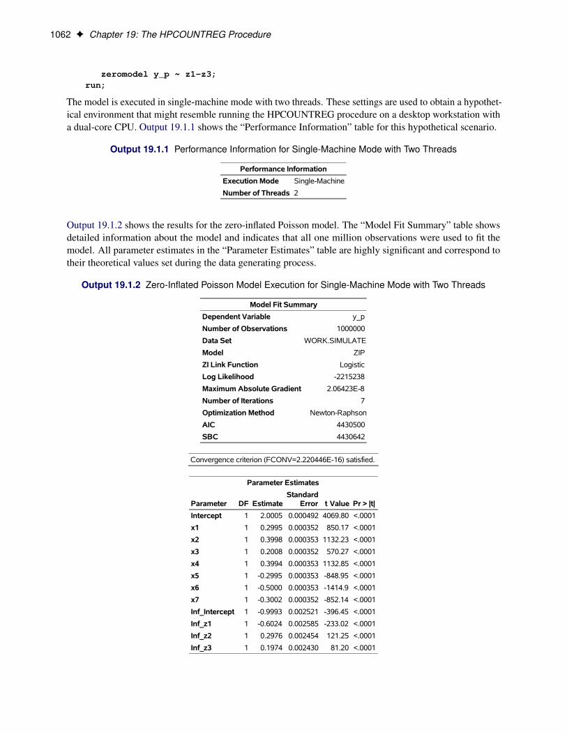
1062 F Chapter 19: The HPCOUNTREG Procedure
zeromodel y_p ~ z1-z3;run;
The model is executed in single-machine mode with two threads. These settings are used to obtain a hypothet-ical environment that might resemble running the HPCOUNTREG procedure on a desktop workstation witha dual-core CPU. Output 19.1.1 shows the “Performance Information” table for this hypothetical scenario.
Output 19.1.1 Performance Information for Single-Machine Mode with Two Threads
Performance Information
Execution Mode Single-Machine
Number of Threads 2
Output 19.1.2 shows the results for the zero-inflated Poisson model. The “Model Fit Summary” table showsdetailed information about the model and indicates that all one million observations were used to fit themodel. All parameter estimates in the “Parameter Estimates” table are highly significant and correspond totheir theoretical values set during the data generating process.
Output 19.1.2 Zero-Inflated Poisson Model Execution for Single-Machine Mode with Two Threads
Model Fit Summary
Dependent Variable y_p
Number of Observations 1000000
Data Set WORK.SIMULATE
Model ZIP
ZI Link Function Logistic
Log Likelihood -2215238
Maximum Absolute Gradient 2.06423E-8
Number of Iterations 7
Optimization Method Newton-Raphson
AIC 4430500
SBC 4430642
Convergence criterion (FCONV=2.220446E-16) satisfied.
Parameter Estimates
Parameter DF EstimateStandard
Error t Value Pr > |t|
Intercept 1 2.0005 0.000492 4069.80 <.0001
x1 1 0.2995 0.000352 850.17 <.0001
x2 1 0.3998 0.000353 1132.23 <.0001
x3 1 0.2008 0.000352 570.27 <.0001
x4 1 0.3994 0.000353 1132.85 <.0001
x5 1 -0.2995 0.000353 -848.95 <.0001
x6 1 -0.5000 0.000353 -1414.9 <.0001
x7 1 -0.3002 0.000352 -852.14 <.0001
Inf_Intercept 1 -0.9993 0.002521 -396.45 <.0001
Inf_z1 1 -0.6024 0.002585 -233.02 <.0001
Inf_z2 1 0.2976 0.002454 121.25 <.0001
Inf_z3 1 0.1974 0.002430 81.20 <.0001
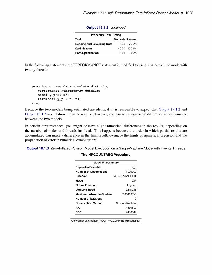
Example 19.1: High-Performance Zero-Inflated Poisson Model F 1063
Output 19.1.2 continued
Procedure Task Timing
Task Seconds Percent
Reading and Levelizing Data 3.40 7.77%
Optimization 40.30 92.21%
Post-Optimization 0.01 0.02%
In the following statements, the PERFORMANCE statement is modified to use a single-machine mode withtwenty threads:
proc hpcountreg data=simulate dist=zip;performance nthreads=20 details;model y_p=x1-x7;zeromodel y_p ~ z1-z3;
run;
Because the two models being estimated are identical, it is reasonable to expect that Output 19.1.2 andOutput 19.1.3 would show the same results. However, you can see a significant difference in performancebetween the two models.
In certain circumstances, you might observe slight numerical differences in the results, depending onthe number of nodes and threads involved. This happens because the order in which partial results areaccumulated can make a difference in the final result, owing to the limits of numerical precision and thepropagation of error in numerical computations.
Output 19.1.3 Zero-Inflated Poisson Model Execution on a Single-Machine Mode with Twenty Threads
The HPCOUNTREG Procedure
Model Fit Summary
Dependent Variable y_p
Number of Observations 1000000
Data Set WORK.SIMULATE
Model ZIP
ZI Link Function Logistic
Log Likelihood -2215238
Maximum Absolute Gradient 2.06483E-8
Number of Iterations 7
Optimization Method Newton-Raphson
AIC 4430500
SBC 4430642
Convergence criterion (FCONV=2.220446E-16) satisfied.
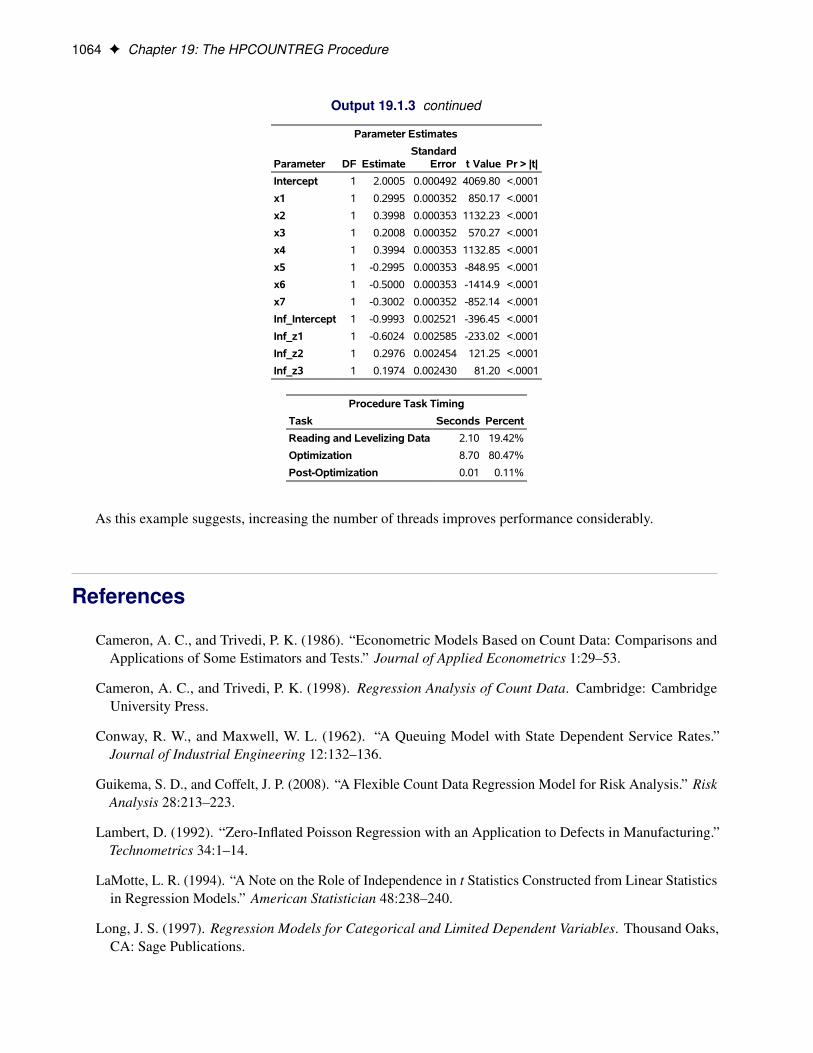
1064 F Chapter 19: The HPCOUNTREG Procedure
Output 19.1.3 continued
Parameter Estimates
Parameter DF EstimateStandard
Error t Value Pr > |t|
Intercept 1 2.0005 0.000492 4069.80 <.0001
x1 1 0.2995 0.000352 850.17 <.0001
x2 1 0.3998 0.000353 1132.23 <.0001
x3 1 0.2008 0.000352 570.27 <.0001
x4 1 0.3994 0.000353 1132.85 <.0001
x5 1 -0.2995 0.000353 -848.95 <.0001
x6 1 -0.5000 0.000353 -1414.9 <.0001
x7 1 -0.3002 0.000352 -852.14 <.0001
Inf_Intercept 1 -0.9993 0.002521 -396.45 <.0001
Inf_z1 1 -0.6024 0.002585 -233.02 <.0001
Inf_z2 1 0.2976 0.002454 121.25 <.0001
Inf_z3 1 0.1974 0.002430 81.20 <.0001
Procedure Task Timing
Task Seconds Percent
Reading and Levelizing Data 2.10 19.42%
Optimization 8.70 80.47%
Post-Optimization 0.01 0.11%
As this example suggests, increasing the number of threads improves performance considerably.
References
Cameron, A. C., and Trivedi, P. K. (1986). “Econometric Models Based on Count Data: Comparisons andApplications of Some Estimators and Tests.” Journal of Applied Econometrics 1:29–53.
Cameron, A. C., and Trivedi, P. K. (1998). Regression Analysis of Count Data. Cambridge: CambridgeUniversity Press.
Conway, R. W., and Maxwell, W. L. (1962). “A Queuing Model with State Dependent Service Rates.”Journal of Industrial Engineering 12:132–136.
Guikema, S. D., and Coffelt, J. P. (2008). “A Flexible Count Data Regression Model for Risk Analysis.” RiskAnalysis 28:213–223.
Lambert, D. (1992). “Zero-Inflated Poisson Regression with an Application to Defects in Manufacturing.”Technometrics 34:1–14.
LaMotte, L. R. (1994). “A Note on the Role of Independence in t Statistics Constructed from Linear Statisticsin Regression Models.” American Statistician 48:238–240.
Long, J. S. (1997). Regression Models for Categorical and Limited Dependent Variables. Thousand Oaks,CA: Sage Publications.
References F 1065
Lord, D., Guikema, S. D., and Geedipally, S. R. (2008). “Application of the Conway-Maxwell-PoissonGeneralized Linear Model for Analyzing Motor Vehicle Crashes.” Accident Analysis and Prevention40:1123–1134.
Shmueli, G., Minka, T. P., Kadane, J. B., Borle, S., and Boatwright, P. (2005). “A Useful Distributionfor Fitting Discrete Data: Revival of the Conway-Maxwell-Poisson Distribution.” Journal of the RoyalStatistical Society, Series C 54:127–142.
Subject Index
BY groupsHPCOUNTREG procedure, 1032
conjugate-gradient optimization method, 1031
double-dogleg optimization method, 1031
HPCOUNTREG procedurebounds on parameter estimates, 1032BY groups, 1032multithreading, 1037output table names, 1060restrictions on parameter estimates, 1038syntax, 1026
multithreadingHPCOUNTREG procedure, 1037
Newton-Raphson optimization method, 1031Newton-Raphson Ridge optimization method, 1031
optimization methodsconjugate-gradient, 1031double-dogleg, 1031Newton-Raphson, 1031Newton-Raphson Ridge, 1031none, 1031quasi-Newton, 1031trust region, 1031
output table namesHPCOUNTREG procedure, 1060
quasi-Newton optimization method, 1031
trust region optimization method, 1031

Syntax Index
ALL optionTEST statement (HPCOUNTREG), 1039
BOUNDS statementHPCOUNTREG procedure, 1032
BY statementHPCOUNTREG procedure, 1032
COPYVAR= optionOUTPUT statement (HPCOUNTREG), 1036
CORRB optionMODEL statement, 1035PROC HPCOUNTREG statement, 1029
CORROUT optionPROC HPCOUNTREG statement, 1028
COVB optionMODEL statement, 1036PROC HPCOUNTREG statement, 1029
COVEST= optionPROC HPCOUNTREG statement, 1029
COVOUT optionPROC HPCOUNTREG statement, 1029
DATA= optionPROC HPCOUNTREG statement, 1028
DETAILS optionPERFORMANCE statement (HPCOUNTREG),
1037DISPERSION= option
OUTPUT statement (HPCOUNTREG), 1037DISPMODEL statement
HPCOUNTREG procedure, 1033DIST= option
HPCOUNTREG statement (HPCOUNTREG),1034
MODEL statement (HPCOUNTREG), 1034
ERRORCOMP= optionHPCOUNTREG statement (HPCOUNTREG),
1035MODEL statement (HPCOUNTREG), 1035
FREQ statementHPCOUNTREG procedure, 1034
GDELTA= optionOUTPUT statement (HPCOUNTREG), 1037
GROUPID= optionPROC HPCOUNTREG statement, 1028
HPCOUNTREG procedure, 1026PERFORMANCE statement, 1037syntax, 1026
HPCOUNTREG procedure, CLASS statement, 1033HPCOUNTREG procedure, PERFORMANCE
statement, 1037HPCOUNTREG procedure, TEST statement, 1039HPCOUNTREG procedure, WEIGHT statement, 1040
INIT statementHPCOUNTREG procedure, 1034
LAMBDA= optionOUTPUT statement (HPCOUNTREG), 1037
LM optionTEST statement (HPCOUNTREG), 1039
LR optionTEST statement (HPCOUNTREG), 1039
METHOD= optionPROC HPCOUNTREG statement, 1031
MODE= optionOUTPUT statement (HPCOUNTREG), 1037
MODEL statementHPCOUNTREG procedure, 1034
MU= optionOUTPUT statement (HPCOUNTREG), 1037
NOINT optionMODEL statement (HPCOUNTREG), 1035
NONORMALIZE optionWEIGHT statement (HPCOUNTREG), 1040
NOPRINT optionPROC HPCOUNTREG statement, 1029, 1036
NTHREADS= optionPERFORMANCE statement (HPCOUNTREG),
1038NU= option
OUTPUT statement (HPCOUNTREG), 1037
OFFSET= optionMODEL statement (HPCOUNTREG), 1035
OUT= optionOUTPUT statement (HPCOUNTREG), 1036
OUTEST= optionPROC HPCOUNTREG statement, 1028
OUTPUT statementHPCOUNTREG procedure, 1036
PARAMETER= option
COUNTREG statement (COUNTREG), 1035MODEL statement (COUNTREG), 1035
PERFORMANCE statementHPCOUNTREG procedure, 1037
PRED= optionOUTPUT statement (HPCOUNTREG), 1036
PRINTALL optionMODEL statement, 1036PROC HPCOUNTREG statement, 1029
PROB= optionOUTPUT statement (HPCOUNTREG), 1036
PROBCOUNT optionOUTPUT statement (HPCOUNTREG), 1036
PROBZERO= optionOUTPUT statement (HPCOUNTREG), 1037
RESTRICT statementHPCOUNTREG procedure, 1038
VARIANCE= optionOUTPUT statement (HPCOUNTREG), 1037
WALD optionTEST statement (HPCOUNTREG), 1039
XBETA= optionOUTPUT statement (HPCOUNTREG), 1036
ZEROMODEL statementHPCOUNTREG procedure, 1040
ZGAMMA= optionOUTPUT statement (HPCOUNTREG), 1037