The Housing Market Effects of Local Home Purchase Restrictions: Evidence from Beijing · PDF...

The Housing Market Effects of Local Home Purchase Restrictions:

Evidence from Beijing

Weizeng SUN

Department of Construction Management & Hang Lung Center for Real Estate

Tsinghua University

[email protected]

Siqi ZHENG

Department of Construction Management & Hang Lung Center for Real Estate

Tsinghua University

[email protected]

David M. GELTNER

Center for Real Estate & Department of Urban Studies and Planning, MIT

[email protected]

Rui WANG*

Luskin School of Public Affairs, UCLA

[email protected]

*Contact information:

3250 Public Policy Building

Box 951656

Los Angeles, CA 90095

Tel +1 (310) 367-3738

Fax +1 (310) 206-5566

December 2014

0

mailto:[email protected]




The Housing Market Effects of Local Home Purchase Restrictions:

Evidence from Beijing

Abstract

Home prices have surged in major Chinese cities, leading to concerns of asset price bubbles and

housing affordability. The policy of home purchase restrictions (HPR) has been one of China’s

harshest housing market interventions to squeeze out speculative demand and dampen the

soaring home prices. Beijing was the first city to implement the HPR. Employing the regression

discontinuity design technique, we find that Beijing’s HPR policy triggered a 17-32% decrease

in resale price, a drop in the price-to-rent ratio of about a quarter of its mean value, and a deep

(1/2 to 3/4) reduction in the transaction volume of the for-sale market, with no significant change

in the rent or the transaction volume of rental units. In submarkets where housing supply was

less elastic, the effects of the HPR were larger in price and smaller in quantity, suggesting that

wealthy buyers likely benefited more from the HPR.

Keywords

Home purchase restriction, housing market, Chinese housing policy, Beijing

1

1 INTRODUCTION

Growing at a nearly 10% average annual rate for three decades, China overtook Japan in 2010 to

become the second largest economy in the world. Urbanization has accompanied the rapid

economic development of China – the proportion of population living in urban areas increased

from less than 20% in 1980 to 52% in 2012. Market-oriented reforms in the urban land and

property markets since the 1990s have replaced the socialist welfare housing regime and

established increasingly competitive housing markets in Chinese cities. Housing demand and

supply have been growing rapidly, becoming a major source for China’s economic growth. The

average amount of floor space per capita among urban households has increased from 21.81 to

29.15 square meters or by 33.6% during the first decade of this century according to national

census data. By late 2009, real estate investment accounted for about 20% of total investment

and around 9% of GDP, with loans to property developers and mortgages together accounting for

about 20% of total loans (Ahuja et al., 2010).

Home prices have surged across Chinese cities, leading to concerns about an asset price

bubble and housing affordability. Currently, home prices are at all-time highs, and have

experienced real price appreciation on a par with or in excess of that realized in other markets

(e.g., the U.S.) that are widely considered to have had housing bubbles (Wu et al., 2012).

Nonetheless, given China’s rapid income growth and large-scale rural-to-urban migration, there

are different opinions about the existence of a national housing price bubble. Higher home prices

may still be broadly in line with the fundamental factors and could be supported by a solid

demand for residential housing (World Bank, 2010). However, many agree that housing price

appreciation in the most expensive metropolitan areas, mainly the big coastal cities, has gone

beyond changes in fundamentals (e.g., Peng et al., 2008; Ahuja et al., 2010; Yu, 2010; Dreger

2

and Zhang, 2013; Wang and Zhang, 2012). In addition, given China’s high income inequality,

concerns about the possible overheating of the market and bubbles are aggravated by the

concerns that lower and middle income households cannot afford to buy an apartment in or close

to the center of large cities (World Bank, 2010).

The Chinese government owns urban land and plays the dominant role in controlling and

managing housing supply, demand, and finance. The urban property markets’ important roles in

economic growth and local fiscal revenue (especially from the land leasehold sales) have led

Chinese policymakers to closely monitor and frequently intervene in the housing market to

maintain its stable growth, especially in light of the subprime mortgage crisis in the US.

Authorities at the national and local levels have adjusted land supply, access to credit, and the

permission to purchase properties alternately to cool and stimulate markets (Chen, 2012; Lu et al.,

2012). However, there have been very few studies of the effects of government interventions in

China’s property markets, especially in local markets.

This research aims to evaluate the effects of home purchase restrictions (HPR), an

unprecedented anti-speculation policy in Beijing. Instead of relying on aggregate housing price

or rent indices, we apply the regression discontinuity design (RDD) technique to a large

transaction dataset of resale and rental housing units in Beijing. We find that resale home prices

dropped by 17-32% immediately after the implementation of the HPR, while rent remained

largely unaffected. As a result, the price-to-rent ratio shrank by about 23-29% of its pre-HPR

mean value. It suggests that the HPR did lower Beijing’s housing price, at least during the initial

years after the HPR. This paper also explores the effects’ intra-city spatial variations associated

with submarket supply condition.

3

The rest of the paper is organized as follows. We introduce the HPR policy in Beijing in

Section 2, followed by descriptions of data and methods in Sections 3 and 4. Section 5 discusses

results. Section 6 concludes the paper with policy implications.

2 HOME PURCHASE RESTRICTIONS IN BEIJING

Beijing, the capital city and a megacity of China, has one of the most heated housing markets in

the country. According to the 2010 census, the urban population of Beijing reached 16.86 million,

including about 64% locally registered residents (i.e., those with local household registration, or

Hukou)1 and 36% unregistered (or non-Hukou) residents. Between 2003-Q1 and 2010-Q1,

Beijing’s housing prices appreciated by nearly 20% per year in nominal terms (Wu et al., 2012).

Recent housing price-to-income and price-to-rent ratios are at their highest levels in Beijing’s

history. By early 2010, estimated price-to-income ratios varied from just below 10 (Lu et al.,

2012) to above 18 (Wu et al., 2012). Wu et al.’s (2012) estimates also indicate an increase in the

price-to-rent ratio from 26.4 in 2007-Q1 to 45.9 in 2010-Q1, suggesting the possibility of a local

housing bubble in development.

As China’s housing markets recovered quickly from the influence of the subprime

mortgage crisis and housing prices kept on rising, the government introduced two rounds of

market regulations in 2010 mainly to deter speculation. On February 21st, the first round of

regulation , hereinafter Policy I, required the down-payment ratio to be a minimum of 40% for

1 Hukou is a resident permit issued to households by the government of China. Every household has a Hukou that

records information about the household members, including name, birth date, relationship with each other,

marriage status (and with whom if married), address and employer. Rural Chinese who migrate to cities are often

ineligible for basic urban welfare and social services due to the lack of a local urban Hukou.

4

the purchase of second homes (a reiteration of a 2007 policy2) and the raise of profit tax rate on

home resale within five years of purchase. Due to the limited effect of Policy I, in April 2010 the

State Council required local governments to impose direct restrictions on home purchases, a

measure considered by many as “the harshest housing market regulation”.3 The larger cities were

urged by the State Council to implement stricter HPR measures and do so more promptly. Two

weeks later, on April 30, 2010, Beijing became the first city to announce and enact immediately

a bundle of policies, hereinafter Policy II.4 The central feature of Policy II was the home

purchase restrictions (HPR), the first command-and-control type regulation on housing demand.

The HPR limits households with a Beijing local Hukou to a maximum of two homes (except that

additional homes already owned were “grandfathered”) while non-hukou households were

simply prohibited from purchasing homes any more.

Accompanying the HPR in the bundle of Policy II there were two additional policies.

One is the further strengthening of Policy I – requiring a minimum of 50% down payment with a

mortgage rate at least 10% above base rate for the purchase of second homed. The other policy is

essentially a reiteration of a national policy enacted in 2007 (see footnote 2) requiring the

minimum down payment ratio to be 30% for a first-home larger than 90 m2 in size. Given the

two policies additional to the HPR in Policy II essentially marginally modified or reiterated

previous policies and were less restrictive than the HPR’s direct command and control, we will

2 On September 27, 2007, People’s Bank of China issued its No. 359 [2007] regulation: “notice of the People’s Bank

of China and China Banking Regulatory Commission on strengthening the management of commercial real estate

credit loans”. 3 According to the State Council’s guidelines, urban households with local Hukou can own up to two housing units,

and non-Hukou households who have been working and paying tax in the city for more than one year can only own

one housing unit. Other urban households were prohibited from purchasing a home. The Beijing restrictions

discussed in this paper are stricter than these national guidelines. 4 By the end of March 2011, 33 cities had imposed the HPR policy.

5

first focus our analysis on the HPR before returning to the two additional policies later in the

paper.

To restrict the speculative housing demand in Beijing, the HPR does not deal with the

factors motivating the speculative demand, and relies on a simple command-and-control of

market entry based on Hukou status and the number of units owned. By restricting the eligibility

to purchase homes to certain groups of people, the HPR significantly and suddenly alters the

demand in Beijing’s housing market, as detailed below.

The HPR brings two direct, first-order impacts on Beijing’s housing market. The first

impact is the dampening of demand for for-sale units as some households are denied access to

the market of for-sale housing, resulting in an exogenous negative demand shock in the for-sale

market. This negative demand shock should lead to clear drops in both price and transaction

volume in the for-sale market, although the impact may be somewhat mitigated after all sorts of

secondary effects kick in. The other first-order impact is the forced shift of some households

from buyers to renters. For households who have housing needs but no local Hukou, including

many young graduates from colleges and universities, the HPR reduces their options to either

becoming renters or leaving Beijing, with the latter a more complicated and longer-term decision.

However, whether and how such a shift of demand from the for-sale market (directly affected by

the HPR) to the connected rental market will affect rents and rental volumes depend on a wide

range of secondary market responses.

There are many possible secondary effects due to the behavioral changes of household

groups indirectly affected by the HPR and the supply-side responses in both the for-sale and the

rental markets. For example, the HPR still allows those households with local Hukou and less

than two homes to buy one home. They may be attracted by the housing price reduction (caused

6

by the first-order demand drop) to buy, or alternatively, they may be discouraged from

speculative purchase if the HPR reduces the expectation of price appreciation and thereby

reduces expected investment returns.5 On the supply side, while the HPR does nothing

fundamentally to stimulate new physical supply of additional housing (the welfare-maximizing

approach to putting downward pressure on home prices), such a policy could actually have a

temporary positive effect on the supply of housing if speculative developers and owners put their

vacant properties into the market as a result of perceived effectiveness of the HPR at dampening

price appreciation. As a result, although rental price and transaction volume would face upward

pressure due to the shift in demand from for-sale to rental housing, an increased supply in rental

housing could offset any upward pressure on rent.

Overall, the implications of the direct demand-side effects are unambiguous for for-sale

home prices and sales volumes (downward). But the effects of the HPR are ambiguous for rents

and volume in the rental market due to the above-noted range of potential secondary effects. The

previous qualitative analysis has important implications for the interpretation of a price drop in

the for-sale housing market in Beijing immediately following the HPR policies. Such a drop

would point to speculation as having played a major role in the increase in for-sale housing

prices in Beijing prior to May 2010, as the speculative demand from owning multiple homes is

the target of the HPR policy. However, any such interpretation would not be air-tight, as directly-

targeted groups were only partially responsible speculative demand. To the extent any post-HPR

price drop resulted from the removal of the owner-occupancy demand by some households (e.g.,

the non-Hukou households owning no home), this does not imply a speculation-based cause of

the previous for-sale home price increases or the price level just prior to May 2010.

5 Other possibilities are plausible given the different expectation effects. For example, if households view the HPR

as a temporary policy, there could emerge a new expectation-based purchase demand.

7

Finally, there is the question of whether and how effects of the HPR may be spatially

heterogeneous within metropolitan Beijing. An exogenous demand shock’s effects on a market

always depend on the supply-price elasticity of a local housing market. Several recent studies

have empirically tested the effects of housing supply constraints (caused by different geographic

conditions or local regulatory regimes) on housing price in different countries (e.g., Glaeser et al.,

2005; Glaeser et al., 2008; Hilber and Mayer, 2001; Paciorek, 2013; Saiz, 2010; Stadelmann and

Billon, 2012). In Beijing, Zheng et al. (2014) find that the capitalization rate of public goods in

home price is larger in supply-constrained locations. We expect that the HPR affects Beijing’s

different housing submarkets differently. More specifically, submarkets with a smaller supply

price-elasticity will show greater price drop and less volume drop following the HPR. This may

have important policy implications about the distributional effects of the HPR. For example, if

housing price is correlated with supply conditions (e.g., housing tends to be more expensive

where there is little room for additional supply), then this suggests that the buyers of expensive

homes probably benefit more from the HPR because affordability is improved more where

supply is less elastic.

3 DATA

We obtain resale and rental transaction datasets from a major broker company “WoAiWoJia”

(www.5i5j.com), the second largest broker in Beijing with a market share of more than 10

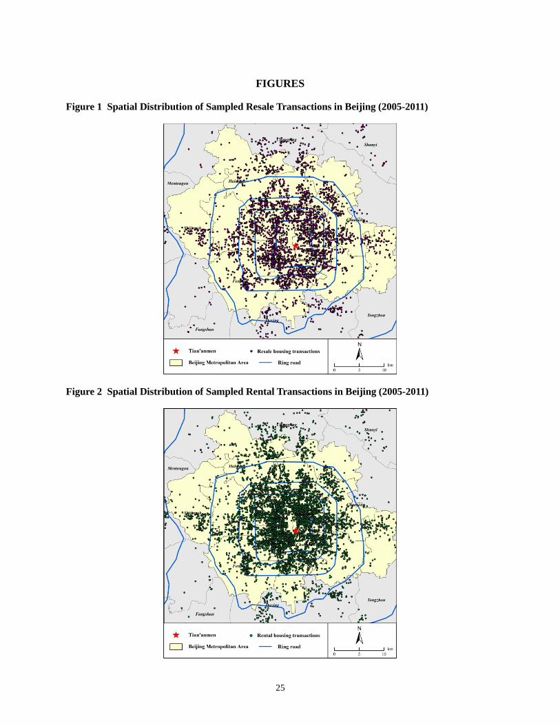
percent.6 Judging from 5i5j.com’s market share and the spatial distribution of sample

transactions (see Figures 1 and 2), we believe their resale and rental transactions can be

approximately considered as representative of the whole market.

6 “Study on the market share of Beijing real estate broker firms (June-October, 2012)” by China Index Academy

(http://fdc.fang.com/report/6115.htm).

8

Figure 1 shows the spatial distribution of all resale transactions conducted by 5i5j.com

during 2005-2011. The effective sample contains 43,305 individual sales in about 3,300

residential complexes. For each transaction record we have the information of transaction date,

exact location, and the housing unit’s physical attributes such as unit size (house_size), age

(house_age), floor number (floor), the number of bathrooms (bathroom) and decoration status in

discrete levels (decoration). The average resale housing unit is 75.45 square meters in size, 14.9

years old, and the mean transaction price (price) is 16,841.2 yuan per square meter in 2005 price.

*** Figure 1 about here ***

Similarly, Figure 2 is a map of all rental transactions. After data cleaning, the rental

transaction dataset has a total of 186,628 observations in about 3,000 residential complexes

during 2005-2011. We have similar variables of rental transactions as for the resale observations.

The average rental housing unit is 63.79 square meters in size (smaller than the average resale

housing units) and the mean monthly rental price (rent) is 46.9 yuan per square meter in 2005

price.7 Within this rental transaction dataset, 13,052 units have repeated transaction records. The

average length of the lease term for those repeated transactions is 0.9 year.


7 The common practice in Beijing is that the landlord pays for the condo fee (property management fee) and winter

heating fee, while the tenant pays utilities and other fees (there is no property tax). The sum of condo fee and winter

heating fee is about 10% to 15% of the gross rent. Also, in Beijing condo fee does not include hazard insurance,

which can be purchased by property owners from insurance companies.

9

We geocode all the resale and rental transactions and calculate the distances of each

residential complex from the city center – Tian’anmen Square (d_center), the closest Key

Primary School (d_school), subway stop (d_subway) and large park (d_park).8

Figures 3-6 plot the temporal distributions of the resale and rental transactions. The red

vertical line in each figure is the announcement/implementation date of Beijing’s HPR policy

(April 30th/May 1st, 2010). The yellow data points are transactions happened in the two weeks

between the announcement of the national guidelines (April 17th, 2010) and the implementation

of Beijing’s HPR policy. A simple visual examination does not suggest any local market

response to the national guidelines prior to the local HPR policy, understandable as Beijing

rolled out its local policy promptly after the national guidelines.

Figure 3 shows the home prices documented in the resale transactions during 2005-2011,

with a clear rising trend from 2005 to the first half of 2010. After the HPR policy (red line), the

growth becomes somewhat stagnant and even negative in 2011. Rent has a relatively wider

cross-sectional distribution than price (Figure 4). It also has a more persistent growth trend

during our study period, with significant seasonal variations.

Our resale and rental datasets overlap in 2800 residential complexes, a large majority of

the complexes in both datasets. The units in a complex share the same architectural design,

location and neighborhood attributes, and they are of the same age, while only differ somewhat

in the physical attributes such as unit size, floor number, and level of decoration. We take

advantage of this high within-complex homogeneity to calculate the complex-level price-to-rent

ratio if a complex has both resale and rental transactions in a week. We divide the average

housing price per square meter by the average monthly rent per square meter of the transactions

8 There are altogether 40 Key Primary (high-quality) Schools, 10 subway lines and 64 large parks in Beijing.

10

in that complex in each week to obtain this ratio.9 Figure 5 shows the distribution of complex-

level price-to-rent ratio and its temporal changes.

Figure 6 plots the transaction volumes of resale units by week. 5i5j.com’s transaction

volume steadily increased from 2005 to the end of 2007 before a significant drop in 2008, most

likely due to the global financial crisis. But starting from early 2009 it began to rise rapidly until

the arrival of the HPR policy, following which there seemed to be a big shrinkage in transaction

volume, although later on it rose and fell again. As with the rental price trend in Figure 4, the

rental transaction volume (Figure 7) shows a clear annual cyclical pattern. Table 1 presents the

definitions and summary statistics of the variables.

*** Figures 3-7 about here ***

*** Table 1 about here ***

4 METHOD

To identify a potential discontinuity in housing market indicators (price, rent, price-to-rent ratio,

and transaction volumes) triggered by the HPR policy, we employ the regression discontinuity

design (RDD) technique for resale and rental prices as specified below:

11

0 1 2 3 41 1 1

log( )K M

ki i k i l li m mi

k l mY HPR Week Month Xβ β β β β ε

= = =

= + ⋅ + ⋅ + ⋅ + ⋅ +∑ ∑ ∑ , (1)

9 Since the number of observations in a complex in a week is usually small, we are unable to run a hedonic

regression to control for physical attributes. Therefore the ratio is calculated with simple averages at the complex-

level.

11

where Yi is unit home price or monthly rent of a transaction observation i,. HPRi equals one if

transaction i happens after April 30th, 2010, otherwise zero. β1 is the primary coefficient of

interest that captures the discontinuity in the dependent variable due to the HPR policy. Vector

β2 captures any pre-existing time trend using a Kth-order polynomial of sequential week numbers

(Week = 1, 2, 3, …). Monthli represents 11 month dummies to capture seasonality. The physical

and location controls Xm capture the cross-sectional differences in housing unit/residential

complex characteristics. β1 represents a constant effect of HPR during the subsequent history in

our data, which is relatively short as it goes only through 2011, less than two years after the

HPR’s implementation. After estimating Equation (1), we can calculate the direction and relative

magnitude of the effect of the HPR on the housing price or rent as 11(%) | 1HPRY eβ=∆ = − .10

Similar RDD regressions are implemented with the price-to-rent ratio (aggregated each

week for complex i) and weekly resale and transaction volumes (i is suppressed in this case) as

dependent variables, although only location characteristics are controlled in the complex-level

price-to-rent ratio regressions and no physical or location control is used in the transaction

volume regressions.11

However, it is difficult to estimate the dynamic effects of the HPR (or any similar

housing market intervention) – whether and how the effects change over time for both data and

modeling reasons. To reliably estimate the HPR’s effect on the housing market over time

requires both information on not just the evolution of market fundamentals, but other relevant

local and national policy interventions during the period of study and a housing market model

10 This is because 1 1 0 1 0 1= log( ) log( ) log( / ) log( (%) | 1)HPR HPR HPR HPR HPRY Y Y Y Yβ = = = = =− = = ∆ + .

11 Although the transactions in our datasets are only part of the whole market, we can still use the RDD technique to

identify the effect of the HPR on transaction volumes, with a reasonable assumption that other factors affecting the

broker’s market share remained unchanged during the short period immediately before and after the implementation

date of HPR policy.

12

sensitive to all policy interventions involved (including perhaps inter-city market interactions),

which could be very complex and methodologically challenging.12 For example, in the long term,

deprived of the option to buy a home, some non-Hukou households at the margin may decide to

move away from Beijing, which may restrict labor supply and hurt the long-term economic

growth and housing demand in Beijing. There could be other side-effects or unanticipated

consequences, such as the behavior of household formation, including possibly an increase in

divorces, a reduction in marriage rate, and/or increased tendency for separate living between the

generations.

5 RESULTS

5.1 City-wide price, rent, and volume effects

We obtain strong and robust city-wide effects of the HPR on the price and volume in the resale

but not the rental market. Table 2 reports a representative set of RDD results.13 Column (1)

provides the regression result for resale housing price. The coefficient of HPR is statistically

significant (0.1% level) and shows a 22.7% (exp(-0.258)-1) drop in housing price after the

implementation of HPR. For the control variables, unit size and house age both have a “U-shape”

relationship with price. The peak value happens around 160 square meters in unit size and 24

12 Polynomial regressions, as adopted in this study, have the ability to approximate a difficult-to-evaluate nonlinear

function, but very limited interpretability. 13 We choose to highlight the results of a tenth-order polynomial time trend because (1) it has a higher adjusted R2

compared to the regressions with other orders of polynomial time trend; and (2) perhaps more importantly, we are

trying to be conservative on identifying the HPR effects, and the higher the polynomial order the easier for the

regression to model changes in the historical market prices in the polynomial, and the more difficult it will be for the

regression to “find” a significant treatment effect of the HPR. Nevertheless, in this paper we also present extensive

robustness checks for alternative specifications including different polynomial orders and time windows.

13

years in age. On the other hand, there is an “inverse-U” relationship between price and floor

number. Housing units on the 6th -7th floor are the most expensive, while units on the top floor

have their price discounted. The number of bathrooms and better decoration contribute to a

higher price. For the location attributes, proximities to the city center, Key Primary Schools and

subway stops all show significant price premiums. Column (2) reports the result for rents. The

coefficient of HPR is also negative (at 0.1% level) and shows a 6.33% (exp(-0.0654)-1) decrease

in rent, much smaller compared to the decrease of housing price. Results for control variables are

similar to those of housing price in column (1). Column (3) shows that after the implementation

of the HPR, the average price-to-rent ratio decreased by 110.1, more than one quarter of the

sample mean ratio of 379.82.


Table 3 reports the RDD estimates with different polynomial time trends. The effects of

HPR on resale housing prices are significantly negative and consistent in magnitude (about a 20-

23% drop). But for the rental market effects, with fifth- and sixth-order polynomial time trends,

HPR has a small positive effect around 3%. However, this effect flips its sign (-5% to -7%) with

higher orders of polynomial time trends. The effect of the HPR on price-to-rent ratio is negative

and statistically significant in all specifications with the coefficient ranging from -85.85 to -110.1,

indicating that the HPR policy suppressed the price-to-rent ratio by about 23- 29% of its mean.


14

The inconsistent estimates of the effects of the HPR on the rental market might result

from the fact that the RDD analysis of the full sample mostly compares the before-and-after-

HPR rents of different housing units, because the terms of rental contracts usually last for the

whole period of lease. To address this problem, we focus on the 13,052 repeated rental

transactions in our sample to compare the longitudinal changes in rent around the

implementation of the HPR. In Table 4, we estimate rent change in time windows of one week,

two weeks and one month on both sides of the HPR. However, we cannot identify a price

discontinuity due to the HPR in the price trend of the rental market as the t-tests cannot reject the

null that there was no difference in the way rents changed around the HPR.14


Table 5 presents the RDD regression results on transaction volumes with different orders

of polynomial time trends. The transaction volume of resale units experienced a huge negative

impact from the implementation of the HPR, with the sizes of magnitude ranging from about

50.9% (exp(-0.712)-1) to 76.7% (exp(-1.458)-1). On the contrary, the rental transaction volume

did not show significant change around the HPR.

14 At the aggregate level, we also obtain similar price and rent effects of the HPR based on the monthly indices of

new and resale price and rent. These aggregate-level analyses use the quality-controlled hedonic monthly price

indices for newly-built houses constructed by the Institute of Real Estate Studies of Tsinghua University for 90

Chinese cities (Zheng et al., 2010) and similar quality-controlled hedonic monthly price and rent indices calculated

using our micro resale and rental transaction data. We find that the effect of the HPR on the new housing price index

is a significant drop of about 12.3-17.3% with multiple orders of time polynomials, while the effects of the HPR on

resale housing price and rent indices are basically the same as the results obtained from the micro data. Results are

available upon request.

15


Table 6 shows the results of the robustness tests using alternative symmetric time

windows: 1.67 years before and after the HPR – the longest symmetric time window allowed by

our data, and one year before and after the HPR, the minimum time window to control for

seasonality. Overall, we get very consistent results about the direction and magnitude of the

resale price effect no matter which time window or polynomial order (once that order is

reasonably high) we use.


In addition, to remove the potential disturbance of Policy I on the effect of the HPR, we

further narrow the time window to February 21st 2010 - June 30th 2010, about 2 months before

and after the HPR. The results for resale housing price and rent are consistent with what we have

found above. But the sample sizes of the transaction volume regressions are too small to produce

reliable results as the narrow time window cannot control for seasonality.

Finally, to explore possible dynamic effects of the HPR, we augment Equation (1) with a

time effect of the HPR as a quadratic term or discrete time dummies. Under each specification,

we also alternate the time units (week, month, and quarter) used.15 However, no clear or

definitive dynamic pattern is identifiable across various polynomial orders and/or time windows.

For example, we cannot say definitively whether the HPR effect was growing or diminishing (or

15 We used alternative time units to model HPR’s dynamic effect, not the overall market trend, which has always

been fitted by polynomials of weeks. The use of time units other than the week and specifications other than the

polynomial alleviates the potential problem of multicollinearity between the market trend and HPR’s dynamic effect.

16

first growing and then diminishing) during the 20 months after the HPR was implemented. But

the main HPR effects remain robust and consistent in magnitude once the polynomial order is

reasonably high.

5.2 Potential effects of simultaneous policies

In Section 5.1 we assume that the HPR dominates the effect of Policy II, which in fact also

includes a further increase in down payment ratio from 40% to 50% for second homes and a

reiteration of a 2007 policy requiring differentiated down payment for homes smaller and bigger

than 90m2.16 While difficult to quantify the precise independent effects of these two policies, we

believe their effects were limited compared to that of the HPR for evidence presented below.

To estimate the effect of the increase in second-home down payment ratio (from 40% to

50%), we notice that Policy I’s main component is such an increase (from 30% to 40%). As

indirect evidence, Table 7 presents the RDD regression results for Policy I using an asymmetric

time window of January 1st 2009 to April 29th 2010 to simultaneously avoid other policies’

effects on housing markets and control for seasonality. Contrast to the significant results of the

HPR (or Policy II), all estimated effects of Policy I are statistically insignificant and much

smaller in magnitude. These results indicate that the increase of down-payment for a second

house may be quite limited, consistent with Chen (2012, pp. 295-296) and in particular Lu et

al.’s (2012, pp. 286-287) observation based on multiple waves of down payment ratio regulations

from January 2005 to May 2010 in Beijing.


16 We thank an anonymous reviewer for detail comments on this issue with helpful suggestions on empirical

strategies.

17

On the other hand, we can directly detect the influence of differentiated down-payment

ratio by home size if it effectively shifted demand to purchase smaller homes. We estimate the

HPR’s effects in markets of different home sizes with specific attention paid to difference around

the demarcation point (90 m2). We spilt the samples into eight groups (<60m2, 60-70m2, 70-80m2,

80-90m2, 90-100m2, 100-110m2, 110-120m2, and >120m2) for the subsample regressions. Table

8 shows the subsample RDD estimates of the effect of the HPR on resale prices with different

polynomial time trends. Estimated HPR coefficients are all negative and statistically significant,

suggesting a market-wide effect of the HPR on resale home price. The estimated HPR effects in

different home size categories ranges from a more dispersed -0.19 (a 17% reduction) to -0.38 (a

32% reduction) with 6th order polynomial time trend to a narrower -0.23 (a 20% reduction) to -

0.35 (a 30% reduction) with 5th order polynomial time trend, compared to the more focused

range of 20-23% reduction estimated using the full sample in Table 3. In particular, there is a

clear trend that the HPR effects become more significant (negatively) with the increase in home

size from the 80-90 m2 category (estimated HPR effects of -0.22 to -0.27 or 20-24% reduction)

to the 100-110 m2 category (estimated HPR effects of -0.35 to -0.38 or 30-32% reduction), after

which the trend is reversed, as shown in Figure 8. In other words, there does seem to be a

significant jump around the 90 m2 threshold due to the differentiated down payment policy.17

While there is no reason to believe that independently the HPR would have an equal

effect in the different home size categories, the effect of differentiated down payment ratios does

seem to coexist with the independent effect of the HPR given the significant boundary

17 Compared to results in Table 7, it seems that the increase in down-payment ratio for first home has more

significant effect on the market than for second home, probably reflecting the difference in demand of the residence

buyers and the speculators.

18

discontinuity at 90 m2. However, given the market-wide significant effect of the HPR, it is

reasonable to claim that the independent effect of the HPR lies in the range of about -0.19 (a

17% reduction) to -0.38 (a 32% reduction), the corresponding lower and higher bounds of the

subsample estimates by home size.



5.3 Spatial heterogeneous effects across submarkets

Our analysis confirms that the HPR’s effects are heterogeneous across submarkets in Beijing

with different supply elasticity. We follow Zheng et al. (2014) to combine three to six adjacent

Jiedaos (Street Offices) with continuous concentrated economic activities into 25 zones as the

basic geographic unit of analysis. Instead of using a direct measure of housing supply elasticity,

we use an exogenous variation in land availability across different locations in Beijing. During

the pre-reform socialist era, state-owned manufacturing enterprises were located across the

central and periphery locations in cities (Zheng et al., 2006). After the reinstatement of the urban

land markets in the late 1980s and especially since the SOE reform started in the late 1990s, the

state-owned manufactures, as large land users, have been gradually moved away from their

original locations. The relocation or disassembly of old state-owned manufacturing firms thus

became an important source of land for new development.18 Zheng et al. (2014) show that the

18 At the end of 1999, the Beijing municipal government announced its plan for manufacturing SOEs’ relocation: in

three to five years from 2000, 738 manufacturing firms within the fourth ring road would be relocated away (see

19

density of state-owned manufacturing employment during the early years of state-owned

enterprise (SOE) reform is statistically correlated with the amount of land leased thereafter and a

valid instrument for land availability.19

We divide the 25 zones into two subgroups – those with lower land availability (lower

SOE employment density in 2000) and those with higher land availability (i.e., higher SOE

employment density in 2000). We estimate Equation (1) using the two subsamples and compare

the subsample effects of the HPR. Table 9 presents the sub-sample RDD regression results. The

HPR policy decreases the resale price by about 23.5% in the zones with relatively inelastic land

supply, larger than its effect in the zones with relatively elastic land supply (21%). A similar

contrast is found in the resale volume effects, with the reduction in resale volume reaching 59%

in submarkets of more elastic supply, compared to the 46% reduction where supply is less elastic.

Two sample t-test results suggest that the intra-city differences in both price and volume effects

are statistically significant at the 0.1% level.


http://house.focus.cn/news/1999-11-03/654.html). According to the plan, the share of industrial land would decrease

from 8.74 percent to 7 percent within the fourth ring road. 19 The correlation coefficient between ln(SOE) (SOE is measured as employment density based on SOE

manufacturing employment numbers by zone from the Year 2000 China Manufacturing Census) and the logarithm

of the amount of land leased during 2006 to 2008 is 0.36 (p-value=0.001). In the meantime, ln(SOE)’s correlation

with ln(home price) is very weak (correlation coefficient is -0.02 for resale housing and 0.06 for new housing) and

statistically insignificant. We have also examined the suitability of historical population density as an exogenous

source of land supply variation but find its validity to be questionable.

20

http://house.focus.cn/news/1999-11-03/654.html

6 CONCLUSION

Home prices have surged in major Chinese cities, leading to concerns of asset price bubbles and

home affordability. China has enacted numerous policies to intervene in its urban housing market,

but there have been few studies evaluating their intended and unintended consequences. The

HPR has been one of China’s harshest housing market interventions to squeeze out speculative

demand and dampen the soaring home prices. Our findings provide early evidence of the HPR’s

effects. Using large datasets of resale and rental market transactions in Beijing and employing

the regression discontinuity design technique, we find that Beijing’s HPR policy triggered about

17-32% decrease in resale price, a decrease in the price-to-rent ratio of 23-29% of its pre-HPR

mean, and a very deep reduction in the transaction volume in the for-sale market, with no

significant change in the rent or the volume of rental units. In submarkets where housing supply

was less elastic, the effects of the HPR were larger in price and smaller in quantity.

A few policy implications arise from our results. A direct interpretation of our results is

that the HPR policy achieved the goal of lowering housing prices without hurting renters (usually

the less wealthy), at least during the 1.67 years of post-HPR time period we have examined. Of

course, to improve housing affordability, simply reducing home prices in the short run may not

help in the long run if it does not reduce the vacancy rate and if it suppresses new construction.

The ultimate evaluation of the HPR’s welfare effect thus depends on whether it helps to get units

occupied (the lack of significant effects in the rental market observed in this study does suggest

the possibility of increased rental supply from previously unoccupied units) and whether it

avoids suppressing new construction. On the other hand, our results that submarkets with less

supply price-elasticity show greater price drop and less volume drop point to the spatially

heterogeneous effect that may be of concern to policy makers. As in many cities, home price is

21

likely correlated with supply conditions in Beijing (e.g., housing tends to be more expensive

where supply is less elastic, such as in the densely developed areas). This means that the buyers

of more expensive homes probably benefit more from the HPR because it triggered a bigger

relative decline (and an even larger absolute decline) in market price in those submarkets.

It should be noted that the HPR’s negative effects on the resale market and price-to-rent

ratio identified in this study are only suggestive about the possibility of the existence and

magnitude of speculative demand in Beijing’s housing market. These results do not represent a

“clean” piece of evidence of the existence of speculative demand, because the owner-occupancy

demand of some non-Hukou households is also curtailed by the HPR policy. In addition, the

HPR cannot prevent speculative purchases by some, especially the Hukou households with one

home. Thus, the HPR effects quantified in this paper may be an underestimate of the magnitude

of speculative demand in this regard.20 Similarly, the lack of significant rental price and volume

impacts cannot be exclusively attributed to an increase in occupancy, a sign of the existence of a

pre-HPR bubble. Overall, one could be more definitive about the existence of a housing bubble if

crucial information such as the change in vacancy and new construction were available. In the

long run, the best policy choice to avoid or curtail excessive speculative purchase of housing

perhaps should be the provision of more alternatives for people to save and invest their money

that offer the prospect of good returns and inflation protection (i.e., development of a more

modern and complete capital market).

20 Likewise, the lack of significant effect in the rental market also cannot suggest a definitive existence of unusually

large number of vacant units (a sign of significant speculation) before the HPR, because some previous renters who

are eligible to buy may move from the rental to the purchase market as a result of the HPR effect on housing prices.

22

REFERENCE

Ahuja, A., Cheung, L., Han, G., Porter, N., & Zhang, W. (2010). Are house prices rising too fast

in China?. IMF Working Papers, 1-31.

Chen, Jie. (2012). Home Mortgage and Real Estate Market in Shanghai. Global Housing

Markets: Crises, Policies, and Institutions. Ashok Bardhan, Robert H. Edelstein, and

Cynthia A. Kroll. Hoboken: John Wiley & Sons.

Dreger, C., & Zhang, Y. (2013). Is there a bubble in the Chinese housing market? Urban Policy

and Research, 31(1): 27-39.

Glaeser, E. L., Gyourko, J., & Saks, R. (2005). Why have housing prices gone up? National

Bureau of Economic Research, No. w11129.

Glaeser, E. L., Gyourkob, J., & Saiz, A. (2008). Housing supply and housing bubbles. Journal of

Urban Economics, 64: 198–217.

Hilber, C. A., & Mayer, C. J. (2001). Land supply, house price capitalization, and local spending

on schools. The Wharton School, University of Pennsylvania,

http://realestate.wharton.upenn.edu/newsletter/392.pdf, accessed 17/12/2010.

Lu, P., H. Zhen, &Y. Xu. (2012). Irrational Prosperity, Housing Market and Financial Crisis.

Global Housing Markets: Crises, Policies, and Institutions. Editors Ashok Bardhan,

Robert H. Edelstein, and Cynthia A. Kroll. Hoboken: John Wiley & Sons.

Paciorek, A. (2013). Supply constraints and housing market dynamics. Journal of Urban

Economics, 77: 11–26.

Peng, W., Tam, D. C., & Yiu, M. S. (2008). Property market and the macroeconomy of mainland

China: a cross region study. Pacific Economic Review, 13(2), 240-258.

Saiz, Albert. (2010). The geographic determinants of housing supply. The Quarterly Journal of

23

http://realestate.wharton.upenn.edu/newsletter/392.pdf

Economics, 125(3), 1253-1296.

Stadelmann, D., & Billon, S. (2012). Capitalisation of Fiscal Variables and Land Scarcity. Urban

Studies, 49(7), 1571-1594.

Wang, Z., & Zhang, Q. (2012). Fundamentals in China’s Housing Markets. Brown University

Working Paper.

World Bank (2010). China Quarterly Update, March.

Wu, J., Gyourko, J., & Deng, Y. (2012). Evaluating conditions in major Chinese housing

markets. Regional Science and Urban Economics, 42(3), 531-543.

Yu, H. (2010). China’s house price: Affected by economic fundamentals or real estate policy?

Frontiers of Economics in China, 5(1), 25-51.

Zheng, S., Fu, Y., & Liu, H. (2006). Housing-choice hindrances and urban spatial structure:

Evidence from matched location and location-preference data in Chinese cities. Journal

of Urban Economics, 60(3), 535-557.

Zheng, S., Kahn, M. E., & Liu, H. (2010). Towards a system of open cities in China: Home

prices, FDI flows and air quality in 35 major cities. Regional Science and Urban

Economics, 40(1), 1-10.

Zheng, S., Sun, W., & Wang, R. (2014). Land supply and capitalization of public goods in

housing prices: evidence from Beijing. Journal of Regional Science, 54(4): 550-568.

24

FIGURES

Figure 1 Spatial Distribution of Sampled Resale Transactions in Beijing (2005-2011)

Figure 2 Spatial Distribution of Sampled Rental Transactions in Beijing (2005-2011)

25

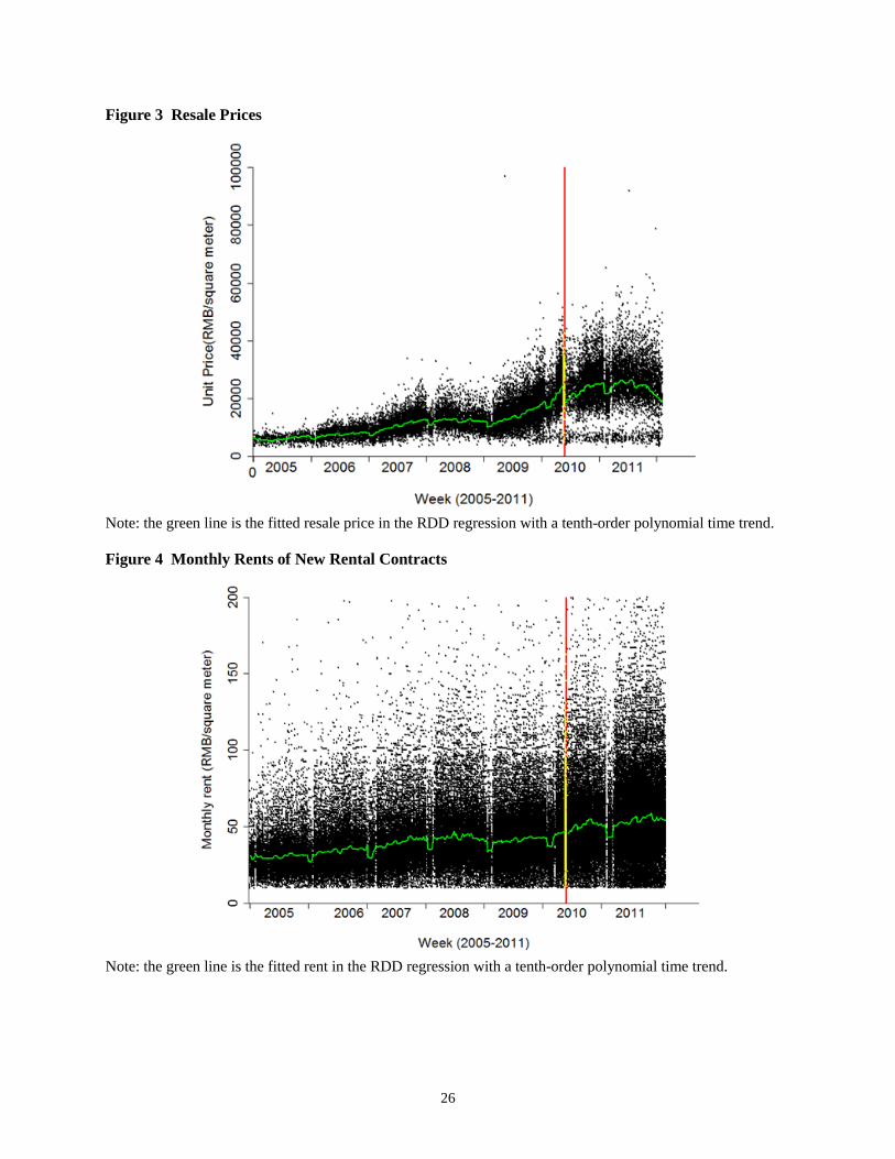
Figure 3 Resale Prices

Note: the green line is the fitted resale price in the RDD regression with a tenth-order polynomial time trend. Figure 4 Monthly Rents of New Rental Contracts

Note: the green line is the fitted rent in the RDD regression with a tenth-order polynomial time trend.

26

Figure 5 Complex-Level Price-to-Rent Ratios

Note: the green line is the fitted price-to-rent ratio in the RDD regression with a tenth-order polynomial time trend. Figure 6 Weekly Resale Volumes

27

Figure 7 Weekly Rental Transaction Volumes

Figure 8 Effects of the HPR by Home Size

-0.4

-0.3

5-0

.3-0

.25

-0.2

-0.1

5

60 70 80 90 100 110 120

Fifth-order Sixth-order Ninth-order Tenth-order

Square meter

28

TABLES Table 1 Variable Definitions and Summary Statistics

Variable Definition Obs. Mean Std.Dev. Min Max Resale Home price

Transaction price (RMB yuan/square meter)

43305 16841.20 7741.39 3069.28 96781.22

house_size Housing unit size (square meter) 43305 75.45 31.33 20.06 199.90 house_age Housing age (years) 43305 14.90 7.64 1 40 floor Floor number 43305 7.94 6.17 1 39

top Whether unit is on the top floor: 1=yes, 0=no

43305 0.12 0.32 0 1

bathroom Number of bathrooms 43305 1.11 0.32 1 3

decoration Decoration level: 1=no decoration, 2=simple decoration, 3=medium decoration, 4=full decoration

43305 2.81 0.99 1 4

Rental Home rent

Monthly rent (RMB yuan/square meter)

186628 46.90 21.56 10 199.88

house_size Housing unit size (square meter) 186628 63.79 31.95 10 200 floor Floor number 186628 7.23 5.86 1 39

top Whether unit is on the top floor: 1=yes, 0=no

186628 0.12 0.33 0 1

living_room Whether unit has at least one living room: 1=yes, 0=no

186628 0.96 0.20 0 1

Price-to-Rent Ratio Quality-controlled price to (monthly) rent ratio, by residential complex by week

13507 425.19 212.57 44.12 1248.486

Location Attributes d_cbd Distance to Tian’anmen Square (km) 3316 8.95 4.69 0.09 25.33

d_school Distance to the nearest key primary school (km)

3316 2.40 1.88 0.01 11.13

d_subway Distance to the nearest subway station (km)

3316 1.69 1.45 0.01 10.58

d_park Distance to the nearest park (km) 3316 1.83 1.23 0.02 8.76

29

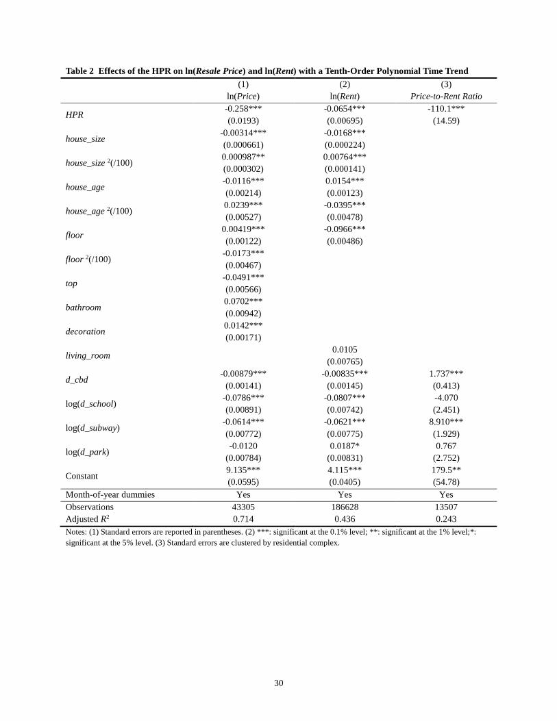
Table 2 Effects of the HPR on ln(Resale Price) and ln(Rent) with a Tenth-Order Polynomial Time Trend (1) (2) (3) ln(Price) ln(Rent) Price-to-Rent Ratio

HPR -0.258*** -0.0654*** -110.1*** (0.0193) (0.00695) (14.59)

house_size -0.00314*** -0.0168*** (0.000661) (0.000224)

house_size 2(/100) 0.000987** 0.00764*** (0.000302) (0.000141)

house_age -0.0116*** 0.0154*** (0.00214) (0.00123)

house_age 2(/100) 0.0239*** -0.0395*** (0.00527) (0.00478)

floor 0.00419*** -0.0966*** (0.00122) (0.00486)

floor 2(/100) -0.0173*** (0.00467)

top -0.0491*** (0.00566)

bathroom 0.0702*** (0.00942)

decoration 0.0142*** (0.00171)

living_room 0.0105 (0.00765)

d_cbd -0.00879*** -0.00835*** 1.737***

(0.00141) (0.00145) (0.413)

log(d_school) -0.0786*** -0.0807*** -4.070 (0.00891) (0.00742) (2.451)

log(d_subway) -0.0614*** -0.0621*** 8.910*** (0.00772) (0.00775) (1.929)

log(d_park) -0.0120 0.0187* 0.767

(0.00784) (0.00831) (2.752)

Constant 9.135*** 4.115*** 179.5** (0.0595) (0.0405) (54.78)

Month-of-year dummies Yes Yes Yes Observations 43305 186628 13507 Adjusted R2 0.714 0.436 0.243 Notes: (1) Standard errors are reported in parentheses. (2) ***: significant at the 0.1% level; **: significant at the 1% level;*: significant at the 5% level. (3) Standard errors are clustered by residential complex.

30

Table 3 Effects of the HPR on ln(Resale Price) and ln(Rent) with Alternative Polynomial Orders (1) (2) (3) (4)

Fifth-order

polynomial time trend Sixth-order

polynomial time trend Ninth-order

polynomial time trend Tenth-order

polynomial time trend

ln(Price) -0.243*** -0.221*** -0.257*** -0.258*** (0.0109) (0.0136) (0.0193) (0.0193) [0.699] [0.699] [0.714] [0.714]

ln(Rent) 0.0279*** 0.0271*** -0.0476*** -0.0682*** (0.00544) (0.00535) (0.00625) (0.00713) [0.433] [0.433] [0.436] [0.436]

Price-to-Rent Ratio

-96.57*** -85.85*** -105.3*** -110.1*** (10.15) (10.47) (14.47) (14.59) [0.235] [0.236] [0.243] [0.243]

Notes: (1) Standard errors are clustered by residential complex and reported in parentheses; adjusted R-squares are reported in square brackets. (2) ***: significant at the 0.1% level; **: significant at the 1% level;*: significant at the 5% level. (3) Control variables are the same as in Table 2. Table 4 Longitudinal Comparisons of ln(Rent) Changes before and after the HPR

Time window Leasing period

adjustment

Pre-HPR mean (Xa) (Std. dev.)

Post-HPR mean (Xb) (Std. dev.)

t-statistic H0: Xa=Xb

(p-value)

Two weeks No

11.56 12.28 0.39 (10.94) (12.04) (0.69)

Yes 16.40 17.11 0.39

(10.66) (11.74) (0.69)

Four weeks No

12.46 11.82 0.56 (11.13) (10.40) (0.57)

Yes 17.26 16.58 0.61

(10.89) (10.21) (0.54)

Two months No

12.18 12.33 0.21 (10.56) (10.14) (0.83)

Yes 16.83 16.99 0.23

(10.36) (10.03) (0.82) Table 5 Effects of the HPR on ln(Volumes) with Alternative Polynomial Orders (1) (2) (3) (4)

Fifth-order


Sixth-order polynomial time

trend

Ninth-order polynomial time

trend

Tenth-order polynomial time

trend

ln(Volume)

Resale -1.458*** -1.282*** -0.966*** -0.712***

(0.183) (0.182) (0.230) (0.219) [0.765] [0.778] [0.784] [0.810]

Rental -0.0858 -0.0837 0.258 0.303 (0.159) (0.163) (0.207) (0.209) [0.570] [0.568] [0.577] [0.578]

Notes: (1) Standard errors are reported in parentheses; adjusted R-squares are reported in square brackets. (2) ***: significant at the 1% level; **: significant at the 5% level;*: significant at the 10% level. (3) Month-of-year dummies are controlled.

31

Table 6 Robustness Tests of the HPR Effects with Alternative Polynomial Orders and Time Windows Time

window [obs.]

Polynomial orders of time trend

1st 2nd 3rd 4th 5th 6th 7th 8th 9th 10th

ln(Price)

3.33 yrs [30,826]

-0.0142 0.0630*** -0.226*** -0.203*** -0.256*** -0.242*** -0.253*** -0.257*** -0.263*** -0.265*** (0.00927) (0.00938) (0.0130) (0.0162) (0.0279) (0.0284) (0.0282) (0.0284) (0.0289) (0.0289) [0.496] [0.553] [0.574] [0.575] [0.575] [0.575] [0.575] [0.575] [0.575] [0.575]

2 yrs [21,613]

-0.0203 -0.0403 -0.245*** -0.235*** -0.233*** -0.231*** -0.240*** -0.239*** -0.240*** -0.237*** (0.0410) (0.0429) (0.0517) (0.0520) (0.0522) (0.0524) (0.0592) (0.0590) (0.0596) (0.0611) [0.475] [0.493] [0.497] [0.497] [0.497] [0.497] [0.497] [0.497] [0.497] [0.497]

ln(Resale Volume)

3.33 yrs [174]

-0.777*** -0.795*** -0.669*** -0.601*** -1.422*** -1.505*** -1.383*** -1.438*** -1.530*** -1.655*** (0.176) (0.159) (0.228) (0.193) (0.310) (0.298) (0.306) (0.309) (0.309) (0.298) [0.255] [0.391] [0.390] [0.562] [0.588] [0.600] [0.604] [0.602] [0.606] [0.641]

2 yrs [106]

-0.937* -0.584 -1.770*** -1.857*** -1.859*** -1.861*** -1.905*** -1.860*** -1.911*** -1.734*** (0.509) (0.475) (0.483) (0.510) (0.514) (0.517) (0.566) (0.569) (0.572) (0.620) [0.475] [0.493] [0.497] [0.497] [0.497] [0.497] [0.497] [0.497] [0.497] [0.497]

ln(Rent)

3.33 yrs [124,111]

0.0615*** 0.0594*** -0.0170** -0.0228*** 0.00428 -0.000513 0.00565 0.00845 0.0155 0.00799 (0.00448) (0.00441) (0.00590) (0.00586) (0.00870) (0.00856) (0.00870) (0.00879) (0.00946) (0.00859) [0.399] [0.399] [0.401] [0.401] [0.401] [0.401] [0.401] [0.401] [0.401] [0.401]

2 yrs [75,010]

0.0384** 0.0258* 0.0266 0.0157 0.0147 0.0138 0.0117 0.0112 0.0118 0.0126 (0.0127) (0.0128) (0.0141) (0.0145) (0.0146) (0.0146) (0.0160) (0.0159) (0.0160) (0.0162) [0.401] [0.401] [0.401] [0.401] [0.401] [0.401] [0.401] [0.401] [0.401] [0.401]

ln(Rental Volume)

3.33 yrs [174]

-0.117 -0.116 -0.104 -0.103 0.0779 0.155 0.0439 0.0430 0.0655 0.0975 (0.141) (0.141) (0.203) (0.204) (0.337) (0.328) (0.337) (0.340) (0.342) (0.344) [0.439] [0.437] [0.433] [0.430] [0.428] [0.430] [0.432] [0.432] [0.431] [0.431]

2 yrs [106]

-0.121 -0.196 0.0725 0.225 0.232 0.238 0.0779 0.0440 -0.00517 -0.248 (0.550) (0.561) (0.636) (0.669) (0.673) (0.678) (0.742) (0.747) (0.749) (0.804) [0.317] [0.313] [0.312] [0.308] [0.308] [0.308] [0.303] [0.303] [0.305] [0.303]

Notes: (1) Standard errors are clustered by residential complex and reported in parentheses; adjusted R-squares are reported in square brackets. (2) ***: significant at the 0.1% level; **: significant at the 1% level;*: significant at the 5% level. (3) Control variables are the same as in Table 2.

32

Table 7 Policy I’s Effects on ln(Price), ln(Rent) and ln(Volumes) (Period: January 1st 2009 to April 29th 2010) (1) (2) (3) (4)

obs. Fifth-order



trend


trend


trend

ln(Resale Price)

17,946 -0.00674 -0.00671 -0.0204 -0.0192 (0.0229) (0.0229) (0.0233) (0.0252) [0.585] [0.585] [0.585] [0.585]

ln(Rent) 45,478 0.00682 0.00677 0.00137 0.00323 (0.0136) (0.0136) (0.0138) (0.0138) [0.412] [0.412] [0.412] [0.412]

Price-to-Rent Ratio

5,650 26.02 25.61 27.84 27.16

(18.56) (18.58) (19.83) (20.16) [0.184] [0.184] [0.184] [0.184]

ln(Resale Volume)

70 0.256 0.242 0.152 0.160

(0.404) (0.405) (0.436) (0.440) [0.531] [0.531] [0.525] [0.524]

ln(Rental Volume)

70 0.713 0.714 0.687 0.728

(0.672) (0.672) (0.684) (0.689) [0.122] [0.122] [0.107] [0.105]

Notes: (1) Standard errors are clustered by residential complex and reported in parentheses; adjusted R-squares are reported in square brackets. (2) ***: significant at the 0.1% level; **: significant at the 1% level;*: significant at the 5% level. (3) Control variables are the same as in Tables 2 (for price/rent/ratio regressions) and 5 (for volume regressions).

33

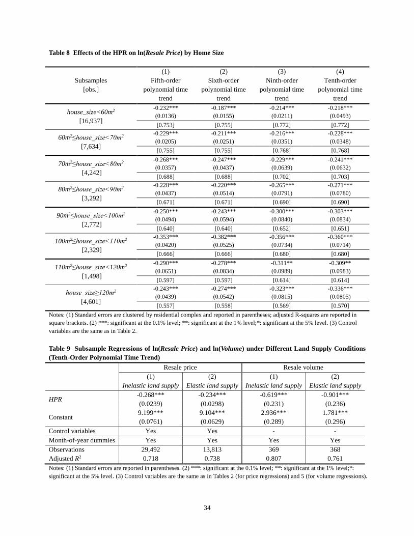
Table 8 Effects of the HPR on ln(Resale Price) by Home Size

Subsamples [obs.]

(1) (2) (3) (4) Fifth-order



trend


trend


trend

house_size<60m2 [16,937]

-0.232*** -0.187*** -0.214*** -0.218*** (0.0136) (0.0155) (0.0211) (0.0493) [0.753] [0.755] [0.772] [0.772]

60m2≤house_size<70m2 [7,634]

-0.229*** -0.211*** -0.216*** -0.228*** (0.0205) (0.0251) (0.0351) (0.0348) [0.755] [0.755] [0.768] [0.768]

70m2≤house_size<80m2 [4,242]

-0.268*** -0.247*** -0.229*** -0.241*** (0.0357) (0.0437) (0.0639) (0.0632) [0.688] [0.688] [0.702] [0.703]

80m2≤house_size<90m2 [3,292]

-0.228*** -0.220*** -0.265*** -0.271*** (0.0437) (0.0514) (0.0791) (0.0780) [0.671] [0.671] [0.690] [0.690]

90m2≤house_size<100m2 [2,772]

-0.250*** -0.243*** -0.300*** -0.303*** (0.0494) (0.0594) (0.0840) (0.0834) [0.640] [0.640] [0.652] [0.651]

100m2≤house_size<110m2 [2,329]

-0.353*** -0.382*** -0.356*** -0.360*** (0.0420) (0.0525) (0.0734) (0.0714) [0.666] [0.666] [0.680] [0.680]

110m2≤house_size<120m2 [1,498]

-0.290*** -0.278*** -0.311** -0.309** (0.0651) (0.0834) (0.0989) (0.0983) [0.597] [0.597] [0.614] [0.614]

house_size≥120m2 [4,601]

-0.243*** -0.274*** -0.323*** -0.336*** (0.0439) (0.0542) (0.0815) (0.0805) [0.557] [0.558] [0.569] [0.570]

Notes: (1) Standard errors are clustered by residential complex and reported in parentheses; adjusted R-squares are reported in square brackets. (2) ***: significant at the 0.1% level; **: significant at the 1% level;*: significant at the 5% level. (3) Control variables are the same as in Table 2. Table 9 Subsample Regressions of ln(Resale Price) and ln(Volume) under Different Land Supply Conditions (Tenth-Order Polynomial Time Trend) Resale price Resale volume (1) (2) (1) (2) Inelastic land supply Elastic land supply Inelastic land supply Elastic land supply

HPR -0.268*** -0.234*** -0.619*** -0.901*** (0.0239) (0.0298) (0.231) (0.236)

Constant 9.199*** 9.104*** 2.936*** 1.781*** (0.0761) (0.0629) (0.289) (0.296)

Control variables Yes Yes - - Month-of-year dummies Yes Yes Yes Yes Observations 29,492 13,813 369 368 Adjusted R2 0.718 0.738 0.807 0.761 Notes: (1) Standard errors are reported in parentheses. (2) ***: significant at the 0.1% level; **: significant at the 1% level;*: significant at the 5% level. (3) Control variables are the same as in Tables 2 (for price regressions) and 5 (for volume regressions).

34

The Housing Market Effects of Local Home Purchase Restrictions: Evidence from Beijing · PDF...

Documents

Transcript of The Housing Market Effects of Local Home Purchase Restrictions: Evidence from Beijing · PDF...