The Håkåneset rockslide, Tinnsjø
172
The Håkåneset rockslide, Tinnsjø Stability analysis of a potentially rock slope instability. Inger Lise Sollie Geotechnology Supervisor: Bjørn Nilsen, IGB Department of Geology and Mineral Resources Engineering Submission date: June 2014 Norwegian University of Science and Technology
Transcript of The Håkåneset rockslide, Tinnsjø

The Håkåneset rockslide, TinnsjøStability analysis of a potentially rock slope
instability.
Inger Lise Sollie
Geotechnology
Supervisor: Bjørn Nilsen, IGB
Department of Geology and Mineral Resources Engineering
Submission date: June 2014
Norwegian University of Science and Technology


I

II

III
ABSTRACT
The Håkåneset rockslide is located on the west shore of Lake Tinnsjø (191 m.a.s.l), a
fjordlake stretching 32 km with a SSE-NNW orientation in Telemark, southern Norway. The
instability extends from 550 m.a.s.l. and down to approximately 300 m depth in the lake,
making up a surface area of 0.54 km2 under water and 0.50 km
2 on land. The rockslide
comprises an anisotropic metavolcanic rock that is strongly fractured. Five discontinuity sets
are identified with systematic field mapping supported by structural analysis of terrestrial
laser scan (TLS) data. These are interpreted as gravitationally reactivated inherited tectonic
structures. At the northern end the instability is limited by a steep south-east dipping joint
(JF3 (~133/77)) that is one direction of a conjugate strike slip fault set (JF3, JF2 (~358/65)).
Towards the south the limit to the stable bedrock is transitional. A back scarp is defined by a
north-east dipping J1 (~074/59) surface that is mapped out at 550 m.a.s.l.
Kinematic analysis indicates that planar sliding, wedge sliding and toppling are feasible.
However, because the joint sets are steeply dipping these failure mechanisms can only occur
for small rock volumes and are limited to steep slope sections only. Large scale rock slope
deformation can only be justified by assuming deformation along a combination of several
anisotropies. This assumption is based on the presence of the ~50-65 degrees NE dipping J1
and the up to 19 degrees NNE dipping foliation, making bi-planar sliding a feasible
mechanism in case of a massive failure of the entire slope instability. Numerical modelling
using Phase2 support assumption of bi-planar failure and indicate that significant rock damage
by retrogressive failure mechanism is most likely for a stepped development of a basal sliding
surface. The modeling results indicate that this sliding surface may daylight at a depth of
~100 m in the lake. By sensitivity tests for groundwater and different joint- and rock mass
properties it is assumed that the instability is, besides the main structures, controlled
principally by topography and rock strength conditions.

IV

V
SAMMENDRAG
Det ustabile fjellpartiet ved Håkåneset er lokalisert på vestsiden av Tinnsjø (191 moh.) i
Telemark i Sør-Norge. Innsjøen strekker seg 32 km i SSØ-NNV retning. Ustabiliteten starter
på 550 moh. og går ned til omtrent 300m dybde i Tinnsjø, og tilsvarer 0,54 km2 under vann
og 0,50 km2 på land. Bergmassen i området består av en en anisotropisk metavulkansk bergart
som er sterkt oppsprukket. Fem sprekkesett er identifisert ved systematisk feltkartlegging, og
har blitt bekreftet med strukturell analyse av "terrestrial laser scan" (TLS). Disse er tolket som
gravitativt reaktiverte tektoniske strukturer. Den nordlige avgrensingen av ustabiliteten er
definert av et bratt sør-øst fallende sprekksett (JF3 (~133/77)) som er tolket som en retning av
et konjugert "strike-slip" forkastningssystem (JF3, JF2(~358/65)). Mot sør er det anslått å
være en gradvis overgang til stabilt fjell. I bakkant er ustabiliteten avgrenset av en bakvegg
med samme orientering som sprekkesettet J1 (~074/59), og reiser seg fra ca. 550 m.o.h..
Kinematisk analyse av diskontinuitetene antyder at planær utgliding, kileformet utgliding og
blokktopling er mulig. På grunn av at det bratte fallet på samtlige sprekkesett er disse
bruddmekanismene mulig kun for små volum og kan kun forekomme i de bratteste delene av
skråningen. For å forklare en massive utglidning av hele fjellpartiet må det antas at
deformasjonen skjer langs en kombinasjon av flere anisotropier. I dette tilfellet er J1 som
faller ~50-65 grader i NØ retning og det opp til 19 grader bratte NNØ fallende foliasjonen to
sprekkesett som gjør bi-planar utgliding av et stort volum av fjell til en mulig
bruddmekanisme. Numerisk modeliering i Phase2 støtter antakelsen om bi-planær utglidning
og indikerer at utviklingen av et nedre bruddplan vil involvere betydeling ødeleggelser av
intakt berg ved en retrogressiv bruddmekanisme. Resultatet fra modeleringen antyder at en
sannsynlig lokalisering av et bruddplanet vil være på et nivå på ca. 100 m dybde i Tinnsjø.
Sensitivitetstest av grunnvann og ulike sprekke- og bergmassestyrkeegenskaper antyder at
stabiliteten av fjellsiden er kontrollert av diskontinuitetene, topografien og bergmassestyrke
paramtre.

VI

VII
PREFACE AND ACKNOWLEDGEMENT
This thesis is the final work of my master degree at the Department of Geology and Mineral
Resource Engineering at the Norwegian University of Science and Technology (NTNU),
Trondheim. The master thesis is written in collaboration with the Norwegian Geological
Survey (NGU). Reginald Hermanns (head of the landslide department at NGU) and Bjørn
Nilsen (professor at the Department of Geology and Mineral Resource Engineering, NTNU)
have been my supervisors.
I would like to thank Bjørn Nilsen and Reginald Hermanns for guiding me through the work
with this master thesis. Thank you for always being so friendly set time for a meeting, to
answer my questions and for all interesting discussions about geology - I have really learned a
lot!
I am also very grateful for the help I have got from Gro Sandøy and Thierry Oppikofer at
NGU and Nghia Quoc Trinh at SINTEF when applying the different software techniques.
Finally, I would like to speak to my classmates at NTNU. Thank you for early mornings and
late night at "Lesesalen", ice cream in the sun, dancing in T-Town, good memories from field
excursions and the years we have had together in Trondheim. You rock!
Trondheim, 10.06.2014
Inger Lise Sollie

VIII

IX
TABLE OF CONTENTS
Abstract ................................................................................................................................... III
Sammendrag ............................................................................................................................. V
Preface and acknowledgement ............................................................................................. VII
Table of Contents ..................................................................................................................... IX
1 Introduction ....................................................................................................................... 1
1.1 Systematic mapping approach of large unstable rock slopes in Norway ........................ 1
1.2 Background .......................................................................................................................... 3
1.3 Aim and restrictions of the study........................................................................................ 3
1.4 Available data and site specific literature .......................................................................... 6
1.5 Previous work ....................................................................................................................... 7
1.5.1 Gvålviknatten rock fall monitoring project, Norwegian Public Roads Administration (Statens
Vegvesen) ...................................................................................................................................................... 7
1.5.2 Periodic monitoring with terrestrial laser scan (TLS), NGU ........................................................... 7
1.5.3 dGNSS displacement measurements (NGU, UiO) .......................................................................... 8
1.5.4 Student project assignment: Geological investigation of Håkåneset ............................................... 8
2 Site information: Regional and geological settings ......................................................... 9
2.1 Location and topography .................................................................................................... 9
2.2 Climate and hydrogeological conditions .......................................................................... 11
2.3 Geology ............................................................................................................................... 14
2.4 Historical events ................................................................................................................. 15
3 General background about large natural rock slope instabilities ................................. 17
3.1 Development and definition of rockslide ......................................................................... 17
3.2 Causes and controlling factors of rock slope instability ................................................. 19
3.3 A case study of a subaerial-subaquatic rockslide: The Hochmais–Atemkopf rockslide
system, Austria ................................................................................................................................ 19
4 Methods used of stability assessment of the Håkåneset rockslide ................................. 21
4.1 Digital elevation model (DEM) analysis ........................................................................... 21

X
4.2 Terrestrial Laser scan (TLS) analyses ............................................................................. 21
4.2.1 Structural analysis in Coltop-3D ................................................................................................... 22
4.2.2 Displacement analysis in Polyworks ............................................................................................. 24
4.3 Stability analysis................................................................................................................. 25
4.3.1 Numerical modeling with Finite Element Method (FEM) of the Håkåneset rock slide ................ 27
5 Results and findings from geological investigation of the Håkåneset rockslide
(Includes results obtained in the project assignment) .............................................................. 31
5.1 Rock mass characterization .............................................................................................. 31
5.1.1 Field observations ......................................................................................................................... 31
5.1.2 Thin section analysis ..................................................................................................................... 32
5.2 Rock mass and discontinuity parameters ........................................................................ 38
5.2.1 Justification of assumed homogeneous material type ................................................................... 38
5.2.2 Rock mass properties .................................................................................................................... 38
5.2.3 Joint sets and structural domains ................................................................................................... 41
5.2.4 Discontinuity strength parameters ................................................................................................. 44
5.3 Major geomorphological features ..................................................................................... 48
5.4 Preliminary findings .......................................................................................................... 50
5.4.1 Lateral limits of the rockslide ........................................................................................................ 50
5.4.2 Results of kinematic feasibility test ............................................................................................... 50
6 The FEM model used for the the Håkåneset rockslide ................................................. 53
6.1 Model geometry set up ....................................................................................................... 53
6.2 Analysis set up .................................................................................................................... 59
6.3 Input parameters for the Håkåneset rock mass .............................................................. 61
6.3.1 Material model and strength criterion of jointed rock mass .......................................................... 62
6.3.2 Material parameters ....................................................................................................................... 65
6.3.3 Discontinuity parameters ............................................................................................................... 70
6.3.4 Stresses .......................................................................................................................................... 79
6.3.5 Hydraulic material properties ........................................................................................................ 81
6.4 Parameter study ................................................................................................................. 82
6.4.1 Model and analyses overview ....................................................................................................... 82
7 Results .............................................................................................................................. 84
7.1 Results from structural analysis of TLS-data in Coltop ................................................. 84
7.1.1 Results from discontinuity mapping in COLTOP ......................................................................... 84

XI
7.1.2 Comparing the results from structural analysis of LiDAR-data with the structural analysis results
based on field measurements ....................................................................................................................... 88
7.1.3 Conclusion .................................................................................................................................... 90
7.2 Results from deformation analysis of TLS-data in Polyworks ...................................... 92
7.3 Results of stability analysis with numerical modeling in Phase2 ................................... 95
7.3.1 Groundwater seepage analysis ...................................................................................................... 95
7.3.2 Effect of submerged-subaquatic instability ................................................................................... 99
7.3.3 Shear strength reduction (SSR) analysis ..................................................................................... 100
8 Discussion ...................................................................................................................... 118
8.1 Geological investigation of the Håkåneset rockslide ..................................................... 118
8.1.1 Structural analysis of field and TLS-data .................................................................................... 118
8.1.1 Recorded slope deformation activity ........................................................................................... 120
8.1.2 Findings from SSR-analysis ........................................................................................................ 121
8.2 Influence of Lake Tinnsjø on the stability of the Håkåneset rockslide ....................... 127
8.3 Volume estimation of the deforming mass in the Håkåneset rockslide ....................... 129
8.4 Uncertainties in the slope stability assessment of Håkåneset rockslide ...................... 132
8.5 Recommendations for further investigations ................................................................ 135
9 Conclusion of the study ................................................................................................. 137
10 References ...................................................................................................................... 139
Appendix ................................................................................................................................... A
A1: Map: Structural orientations, lateral limits, locations (Project assignment) ...................... A
A2: dGNSS measurements (2012,2013), NGU, UiO ....................................................................... B
A3: GSI estimate of the Håkåneset rock mass............................................................................... C
A4: Stereographic pole plots for structural domains .................................................................... D
A5: Normal stress calculation to potential failure surface ............................................................ E
A6: Rock mass strength conversion in RocLab .............................................................................. F
A7: Calculation of joint stiffness ..................................................................................................... G
A8: Phase2 contour plots ................................................................................................................. C
A9: Geometry for volume calculations ............................................................................................ F

XII

Chapter 1 Introduction
1
1 INTRODUCTION
1.1 Systematic mapping approach of large unstable rock slopes
in Norway
The Geological Survey of Norway (NGU) carries out the systematic geologic mapping of
potentially unstable rock slopes in the Norway, while the Norwegian Water Resources and
Energy Directorate (Norges vassdrags- og energidirektorat, NVE) is the finically responsible
for this work (Hermanns et al., 2014). The systematic mapping has been carried out since
2005, were three of the 17 counties of Norway have been prioritized. By now, more than 300
unstable or possible unstable slopes have been found in Troms, Møre og Romsdal and Sogn
og Fjordane (Hermanns et al., 2013). Due to this high number of instabilities, a hazard and
risk classification system has been considered necessary. The established classification
system gives guidelines for a systematic mapping that focuses on the geological data that is
considered as relevant in order to effectively assess qualitatively the likelihood of failure of
unstable rock slopes. Consequently, a hazard and risk classification system is fundamental in
order to establish a database that allow to compare hazard and risk of unstable rock slopes
from all over the country (Bunkholt et al., 2013). Such a database is required in order to
prioritize time and resources for further investigation and follow-up activities on the most
critical unstable slopes.
The Håkåneset rockslide is the first rockslide in Norway where detailed mapping show that
the instability has a combination of a subaerial and a subaqueous component. It is one of 56
sites where periodical displacement measurements are carried out every year or in fixed
yearly intervals by NGU. The interest for periodically measure displacement on this specific
slope is based on the observations of geological features that indicate significant post-glacial
deformation in the rock slope. Due to signs of deformation the Håkåneset rock slope is
considered as a site which might have the potential to fail catastrophically in the future. By
definition a catastrophic failure refers to a fast event with substantial fragmentation of the
involved rock mass during the run and that impacts an area larger than that of the depositional
angle of rock falls (Hermanns and Longva, 2012). Consequently, a catastrophic rock slope
failure has the potential to cause severe material damage and loss of lives.

Chapter 1 Introduction
2
The hazard analysis provided by NGU (Hermanns et al., 2013) is based on two main steps:
First a structural site investigation is undertaken in order to map out morphological
expressions of deformation such as development of a back-scarp, lateral boundaries and basal
sliding surface, and collect a statistical significant data set of orientation measurements of
discontinuities in the assumed unstable rock mass. Further, a kinematic analysis of the
structural data is performed, in order to investigate the feasibility for sliding and toppling
failure based on slope orientation, persistence of main structures and morphologic expressions
of the sliding surface. The geological investigation of the Håkåneset rockslide was undertaken
by the candidate in a project assignment in the autumn semester 2013. The results from that
work indicate that several failure mechanisms are kinematically feasible.
The second step in the hazard analysis involves analysis of slope activity primarily based on
slide velocity, change of deformation rates, observation of rockfall activity, and historic or
prehistoric events. These are factors that will be investigated in this master thesis by analysis
of data obtained by terrestrial laser scanning (TLS) from the Håkåneset rock slope. In
addition, the master thesis includes a structural analysis of TLS data where the aim is to
confirm the structural model obtained by field measurements.
In order to improve the kinematic model of the Håkåneset rockslide a stability analysis by
numerical modeling of the instability has been performed. With numerical modeling
important factors such as persistence of main discontinuities, geotechnical properties of the
rock mass, persistent morphological features and the effect of a submerged toe have been
included in the analysis. All results from the undertaken work serve as a basis for the
discussion of a stability model of the subaerial-subaqueous Håkåneset rockslide.
Chapter 2 presents regional and geological settings for the study area. In Chapter 3 some
general aspects about large rock slope instability are defined. Next, Chapter 4 gives
background information about the methods used in this study. Chapter 5 is important as it
presents the most important results and interpretations from the geological investigation that
are essential for the further stability analysis undertaken in this master thesis. A numerical
modeling with the finite element method (FEM) is a major part of this thesis. Justification of
the applied FEM model and the obtained results are presented in Chapter 6 and Chapter 7,
respectively. Chapter 7 also includes result from structural analysis and deformation
measurements undertaken with TLS data of the study area. Interpretations and discussion of
all results obtained with the applied stability assessment techniques can be read in Chapter 8.

Chapter 1 Introduction
3
Experiences from the geological investigation are discussed to justify interesting results. A
brief volume estimate for the deforming rock mass is calculated and suggestions for further
work are given. Chapter 10 summarizes in short what is considered as the most important
experiences from the undertaken study of the Håkåneset rockslide.
1.2 Background
Mapping large unstable rock slopes is an important work for the society as it helps to detect
rock slopes that might fail catastrophically in future. Catastrophic rock slope failures have
been experienced several times in the steep topography and high relief landscape in Norway,
causing loss of lives and property (Blikra et al., 2006; Hermanns et al., 2012a). Such events
will also occur in the future. It is important to remember that in most cases the rock slope
failures are not the direct causes for the loss. Often the negative consequences to society are
due to resulting displacement waves which run up along the shoreline, after being generated
by the impact of the rockslide body into either a fjord or lake (Harbitz et al., 1993). Therefore,
unstable rock slopes in Norway present a higher threat than in other mountain environments
in the world because settlement and communities in Norway are concentrated along the coast
line of the fjords and mountain lakes (Hermanns et al., 2012a).
The Håkåneset rockslide is located directly along the shore of the lake Tinnsjø in Telemark in
southern Norway, and the instability has both a subaerial and subaqueous component. Thus, a
rapid failure of this rock slope has the potential to cause a displacement wave. A potential
displacement wave in Tinnsjø can reach the settlements in the multiple communities located
around the lake and cause loss of life and property there. Therefore a hazard and risk
classification of the Håkåneset rockslide site is considered as necessary.
1.3 Aim and restrictions of the study
The aim of this master thesis is to perform a stability assessment including numerical
modeling of the unstable rock slope at Håkåneset, in order to provide information that will be
used to discuss different failure scenarios of this unstable slope. The results from this master
thesis provide information that will be used by the Norwegian Geological Survey (NGU) to

Chapter 1 Introduction
4
improve the monitoring network and to contribute to the hazard and risk classification of the
Håkåneset rockslide. The exact classification will not be carried out in this master thesis.
A kinematic model and a simple preliminary stability model of the Håkåneset rockslide exists
as an introductory project assignment conducted by the candidate in the autumn semester
2013. However, a more comprehensive stability analysis, taking into account important
effects like scaling due to non-persistent discontinuities, rock mass strength in relation to
failure of rock bridges and shearing of joint irregularities and the effect of a submerged toe, is
required before the instability of the Håkåneset rockslide can be assessed satisfactorily.
This master thesis particularly focuses on:
1. Reducing the uncertainty of the existing preliminary structural model of the
Håkåneset rockslide by supplementary structural analysis of LiDAR (LIght
Detection And Ranging) -data (aerial laser scans (ALS) and terrestrial laser
scans (TLS)) in COLTOP 3D.
2. Reduce the uncertainties of the kinematic model discussed in the project
assignment and discuss a stability model of the Håkåneset rockslide, by
including joint surface conditions and rock mass properties in the analysis.
This is obtained by defining a structural profile along the slope selected that
area interpreted to be most critical regarding the stability of the slope, which
are used for:
Calculation of stress distribution and Factor of Safety in various parts
of the rock slope by numerical modelling techniques in Phase2
(Rocscience), in order to detect the most likely failure surfaces.
Including the effect of the water within the lower part of the slope in
the stability analysis.
Measuring deformation of the rock slope by the use of land based TLS
in PolyWorks.
Combining the structural profile of the rock slope and deformation
measurements for volume estimations.

Chapter 1 Introduction
5
Adjustment of the thesis description
Some adjustments are made on the original thesis description in consulation with the main
supervisor Bjørn Nilsen. The adjustments are:
1. Only one topographic profile is used for the numerical model. This was decided
because it was evaluated to be important to focus the analyses to what is considered as
the most critical area.
2. Limit equilibrium modelling has not been used in this study. A numerical model with FEM
was suggested by the main supervisor as the best approach of this study due to the pre-known
information about the study area.
3. The undertaken deformation measurement did not give sufficient information for carry out a
volume calculation. However, volume estimation is performed based on the numerical
modeling results and interpretation of a digital elevation model (DEM) of the study area.

Chapter 1 Introduction
6
1.4 Available data and site specific literature
An overview of data from the Håkåneset rockslide site available for the master thesis is listed
in Table 1 below.
Table 1: Available site specific data from the Håkåneset rockslide used in this master
thesis.
Available data from the Håkåneset site: Source
Gvålviknatten rock fall monitoring reports from
2002/2003 and 2006.
(Frisvold, 2006, 2007)
1x1m resolution elevation model from Airborn
Laser Scanning LiDAR data
Statens Kartverk
Bathymetric data NGU, Eilertsen (2013)
High resolution TLS data from 2011, 2012 and
2013
NGU
Air photos of the Håkåneset site Statens Vegvesen
Deformation measurements obtained by Global
Navigation Satellite System (GNSS) from 2012
to 2013
(Eiken, 2013)
Project assignment: Håkåneset, Tinnsjø -
Geological investigation of potentially rockslide.
(summarized in Chapter 5)
(Sollie, 2013)
Chapter 1 Introduction
7
1.5 Previous work
1.5.1 GVÅLVIKNATTEN ROCK FALL MONITORING PROJECT, NORWEGIAN
PUBLIC ROADS ADMINISTRATION (STATENS VEGVESEN)
Highway 37, Tinnsjøvegen, cuts through the unstable rock slope at Håkåneset, and is a road
that regularly experiences rockfall activity. The "Gvålviknatten rockfall monitoring project"
was started by the Norwegian Public Roads Administration (Statens Vegvesen, SVV) in 2001,
with the aim to establish systematic displacement monitoring of bedrock, blocks and soil by
the application of air photos of areas with frequent rock fall activity along the road (Frisvold,
2006, 2007). In addition, GPS control points were installed on selected outcrops for regular
displacement measurements. In particular an exposed outcrop of dissected rock, 200 m above
the highway, named Gvålviknatten (see Appendix 1), was in focus of the project.
Gvålviknatten is located in the central part of the defined limits of the study area. Two GPS
points that were installed on the block area of Gvålvikknatten indicate displacement of
3.1±0.8 cm horizontally and 0.6 ± 0.2 cm vertically from 2003 to 2006. This correspond to a
yearly rate of 10 mm horizontally and 2 mm vertically, which will be within the accuracy
interval of GPS measurements (1-2 cm horizontally and 2-3 cm vertically). The project did
not detect any critical areas that require continuous monitoring. The Gvålviknatten monitoring
project is not in any progress by SVV itself at present time (Langelid, 2013).
1.5.2 PERIODIC MONITORING WITH TERRESTRIAL LASER SCAN (TLS), NGU
During the elaboration of the national hazard mapping plan for Norway, the county geologist
of Telemark, Sven Dahlgren, suggested the unstable area in Håkåneset along Tinnsjø as a
potential high risk site. The national systematic mapping project by NGU initially focused on
the three counties Troms, Møre og Romsdal and Sogn og Fjordane, and therefore the
Håkåneset site was included in a "rest Norway "-project. During the first recognition to the
Håkåneset site it was decided as necessary to define the lateral limits of the instability with
further investigations. TLS has been carried out in 2011, 2012 and 2013. The first year the
survey was obtained from the road with a scanner that has an operative range of
approximately 600 m. However, since 2012 the scanning has been set up at two different
localities in a distance of approximately 2.5 km from the opposite side of Lake Tinnsjø.

Chapter 1 Introduction
8
1.5.3 DGNSS DISPLACEMENT MEASUREMENTS (NGU, UIO)
Displacement measurements of the Håkåneset rockslide have been undertaken by the
Norwegian Geological Survey (NGU) on a yearly basis since 2012 (June 2012 and June
2013). The work is performed in cooperation with the Department of Geoscience at the
University of Oslo (UiO). Measurements are obtained with a Topcon two-frequent GNSS
(Global Navigation Satellite System) by registration of the displacement vectors between two
rover points within the instability and two fixed points (TIN-1 and TIN-2) along the highway
(see Appendix 1). The rover points were installed on what is described as "relative big
blocks" (Eiken, 2013). The study area at Håkåneset is heavily vegetated, which make it
challenging to obtain measurements of satisfactorily quality.
The results from the first year of monitoring are given in Appendix 2. Rover point TIN-1 is
located at Gvålviknatten, while rover point TIN-2 is located in the most upslope exposed
block area within the study area (see Appendix 1).
By experience, significant values for rockslide displacement monitoring are 1-3 mm for
horizontal displacement and 2-6 mm for vertical displacement (Eiken, 2013). Significant
displacement is only measured at TIN-2 (Appendix 2), where a horizontal displacement of 9
mm is registered. The direction of this significant displacement is in WSW-direction, i.e.
directed into the slope.
1.5.4 STUDENT PROJECT ASSIGNMENT: GEOLOGICAL INVESTIGATION OF
HÅKÅNESET
A detailed study of the Håkåneset rockslide was performed as a project assignment conducted
by the candidate of this master thesis in the autumn semester 2013. The work included
mapping of geomorphology, structural geology and geotechnical parameters, laboratory work
for estimation of rock mass strength parameter, kinematic feasibility test and discussion of a
simple preliminary stability model of the Håkåneset rockslide. Important observations and
results obtained during the project assignment are presented in Chapter 5, and serve as a basis
for the further stability analysis performed in this master thesis.

Chapter 2 Site information
9
2 SITE INFORMATION: REGIONAL AND GEOLOGICAL
SETTINGS
2.1 Location and topography
The Håkåneset rockslide is located at the north-west shore of Lake Tinnsjø in the county
Telemark in southern Norway. Tinnsjø stretches 32 km with a SSE-NNW orientation, 191
meter a.s.l (Dons and Jorde, 1978). The unstable rockslope is a combined subaerial and
submerged slope in the foot of the mountain Håkåneset. The mountain goes up to 1249
m.a.s.l. In the project assignment the instability was identified to extend from approximately
300 meters depth in Tinnsjø and up to 550 m.a.s.l on the subaerial mountain slope.
The topography in Telemark is characterized by deeply eroded U-shaped glacial valleys, with
an increasing relief from east to west. The main valleys in Telemark were formed in the
Quaternary by erosion that cut down into the old paleic surface (Jansen, 1986), which is the
pene plane of the original Mesoproterozoic Sveconorwegian orogen of the Fennoscandian
Shield (Viola et al., 2009). Glacial processes followed these primary erosional features and
Figure 1: The unstable rock slope in this study is located at the foot of the Håkåneset Mountain, on a
ENE facing slope along the shore of the lake Tinnsjø. This shaded relief model is derived from a
10x10 m resolutions DEM model.

Chapter 2 Site information
10
formed deep U-shaped valleys. The deglaciation of the Scandinavian Ice Sheet started in the
Old Dryas, about 18,000 years ago. Tinnsjø was at the ice margin approximately 10 600 years
ago(Figure 2, Ramberg (2008)).
The orientation of Tinnsjø is parallel to the main glacial movement direction during the last
glacial maximum in the area,Figure 3. In glacially eroded mountain setting valley profiles
have extra deep submersions downstream meeting points of two or more valleys. In such
areas the merging of several valley glaciers increases the erosion effect, causing deep
thresholds (Jansen, 1986). Today these thresholds are filled with water and forming lakes
such as Lake Tinnsjø, which is located south of five merging valleys. Tinnsjø is measured to
be up to 460 m deep (http://www.nve.no/).
Figure 2: Map showing the stages of the
retreat of the Scandinavian Ice Sheet. Ages
for the various position of the ice margin
are shown in thousands of calendar years.
Tinnsjø (yellow star) was at the ice margin
approximately 10 600 years ago (outlined
with yellow line). The line marked "12.5-
11.6" (blue) denotes the outer limit during
the Younger Dryas stadial. (ed. after J.
Kleman and A. Strømberg published by
Ramberg (2008).
Figure 3: Extracted section of glacial map of
Norway showing the main glacial movement (black
arrows) in the area of the study area The
Håkåneset rockslide is located at the west shore of
Tinnsjø, outlined in red. (Holtedahl and Andersen,
1960)

Chapter 2 Site information
11
2.2 Climate and hydrogeological conditions
There are no detailed sources or maps of the local hydrogeological conditions of the study
area. In order to get an impression of the regional climate and hydrogeological conditions in
Telemark, regional maps published at seNorge.no have been studied. seNorge.no is an open
portal on the Internet that shows daily updated maps of snow, weather and water conditions
and climate in Norway.
Ground water
Norway’s national catchment database is called REGINE, established and maintained by
Norwegian Water Resources and Energy Directorate (NVE). REGINE divides Norway into
major and subordinate reference units along the coastline, rivers and catchments, where the
subdivision defines the structure in the hydrological system. Maps and information are
provided at (atlas.nve.no).
To get an impression of the local hydrogeological conditions of the study area, the
hydrogeological map of the Tinnsjø REGINE unit (no. 016.G42) was studied, see Figure 4.
The Tinnsjø unit is a part of catchment of Skien ("Skienvassdraget"), and covers an surface
area of 23.15 km2. On average the seepage is 13.27 mill m
3/yr based on measurements in the
Figure 4: Extraction of hydrogeological map of the study area
(atlas.nve.no). No particular conditions are reported within the limits
of the study area.

Chapter 2 Site information
12
period 1961-1990 (atlas.nve.no). North of the instability of the Håkåneset rockslide is
Bjørnebekken, which is the drainage channel of several mountain lakes at the Håkåneset
mountain plateau that is located directly above the instability. Also, in the south of the study
area there are two topographical depressions that are possible drainage channels.
Precipitation
The normal annual precipitation in the region of the study are is 1500-2000 mm, based on
climate registrations in the period 1971-2000, see Figure 5 (www.senorge.no).
Temperature and permafrost
Permafrost thaw is thought to be an important mechanism through which climate controls
slope stability (Gruber and Haeberli, 2007). Figure 6 is a regional map showing the normal
annual temperature in Southern Norway (1971-2000) extracted from the national climate
database at (www.senorge.no). Tinnsjø is located within the red box, thus in a climate region
where the annual mean air temperature is around zero degree. Consequently, conditions
related to permafrost and slope stability is not important for the study of the Håkåneset
rockslide.

Chapter 2 Site information
13
Water level in Tinnsjø
The Håkåneset rockslide is directly in contact with Lake Tinnsjø, which implies that the
groundwater table in the slope will be sensitive to fluctuations in the lake surface level. Due
to the last statutory regulation of the Tinnsjø lake dated to 17.11.2006, maximum fluctuations
of ± 4m is allowed (Østhus, 2012).
Figure 5: Regional map showing the normal
annual precipitation (1971-2000) in Southern
Norway(www.senorge.no). Tinnsjø is located
within the red box. Thus the normal annual
precipitation in the study area can be expected
to be 1500-2000 mm.
Figure 6: Regional map showing the normal
annual temperature in Southern Norway
(1971-2000) (www.senorge.no). Tinnsjø is
located within the red box, thus in a climate
region where the annual temperature is around
zero degree.

Chapter 2 Site information
14
2.3 Geology
The so called "Telemarksuiten" is dominated by rock of Precambrian age (Jansen, 1986).
These are metasediments and metavolcanic rocks. The Håkåneset rockslide is located within
the lowest geological unit "Rjukangruppen", which is characterized by metarhyolite and
metamorphosed tuff, some quartzite and conglomerates/agglomerates (Dons and Jorde, 1978).
Figure 7 gives the location of the study area (red box) on a lithological map (geo.ngu.no). The
Precambrian bedrock in Telemark is in general dissected by several faults and joint sets that
are the result of different deformation phases in the geological history, where characteristic
main sets have a SW-NE and NW-SE orientation (Jansen, 1986).
In Figure 7 it is seen that directly on the opposite side of the lake (at the north-east shore) to
the study area several bands of amphibolites, metagabbro and amphibolgneiss are mapped
(geo.ngu.no). These bands are trending south-west, i.e. in the direction of the study area, and
Figure 7: N250 map showing the regional main bedrock types around Tinnsjø. The study
area(outlined with red the box) is located within a metarhyolitic/metamorphic tuff unit
(geo.ngu.no).

Chapter 2 Site information
15
therefore bedrock of the latter mentioned types can also be expected to be found within the
study area of the Håkåneset rockslide even though they are not mapped out.
The bedrock in the study was further identified during the geological investigation undertaken
by the candidate. Important observations are presented in Chapter 5.
2.4 Historical events
Historical data about the spatial distribution of gravitational slope processes in Norwegian
mountain slopes are vital information when assessing the likelihood of new rock slope
failures in an area. Statistically, areas where a large activity is recorded in historical times
have a higher likelihood to experience new events in the future (Blikra et al., 2006). The
Norwegian Water Resources and Energy Directorate (NVE) provide a historical geohazard
database (Skredhendelsesdatabasen), with information about all historically recorded
geohazards in Norway. By definition, a geohazard event in this database is an event that has
caused damage of life and property (www.nve.no).
A high number of gravitational slope processes events are recorded along the shore of Tinnsjø
(Figure 8). The highest concentration of events is along the west shore of the lake, where also
the study area is located. 220 events are recorded here (www.nve.no). These are mainly rock
fall events. The high frequency of recorded events at the west shore compared to the east
shore of the lake can be explained with a combination of two effects related to construction of
Tinnsjøvegen: 1) a high number of events due to undercutting of the natural slope, and 2)
frequently records of events by road authorities.
37 gravitational slope processes events are registered within the study area of the Håkåneset
rockslide, where 35 are rock fall events, seeFigure 9. The records within the study area are
dated from 1993 - 2013.

Chapter 2 Site information
16
Figure 8: Recorded historical l landslide and rock fall activity
along Tinnsjø (www.nve.no)
Figure 9: 35 historic rock fall events are recorded within the
study area of the Håkåneset rockslide (www.nve.no).
Chapter 3 Theory
17
3 GENERAL BACKGROUND ABOUT LARGE NATURAL ROCK
SLOPE INSTABILITIES
3.1 Development and definition of rockslide
A rockslide is by definition a landslide that involves movement of rock material (e.g Hungr
et al. (2012)). According to Terzaghi (1950) and Leroueil et al. (1996) in Hungr et al. (2012)
is a landslide a mechanical system that develops in time through several stages. These stages
of mass movement may be divided in pre-failure deformations, the failure itself and post-
failure displacements (Skempton and Hutchinson, 1969). Hungr et al. (2012) purposes the
following definition of the term "failure":
"Failure is the single most significant movement episode in the known or anticipated history
of a landslide, which usually involves the first formation of a fully-developed rupture surfaces
as a displacement or strain discontinuity."
When assessing a possible landslide it
is essential to evaluate what stages that
dominates in the unstable slope, as it
may help to predict future behaviour
and explain kinematic trends. In
addition, it may help to obtain more
reliable estimates of material properties
as the degree of strength loss during
deformation and failure (e.g. peak, vs.
residual strength) can be taken account
of. The Håkåneset rockslide is
anticipated to be in the pre-failure
stage.
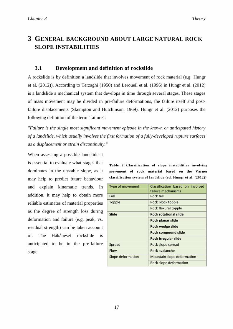
Table 2 Classification of slope instabilities involving
movement of rock material based on the Varnes
classification system of landslide (ed. Hungr et al. (2012))
Type of movement Classification based on involved failure mechanisms
Fall Rock fall
Topple Rock block topple
Rock flexural topple
Slide Rock rotational slide
Rock planar slide
Rock wedge slide
Rock compound slide
Rock irregular slide
Spread Rock slope spread
Flow Rock avalanche
Slope deformation Mountain slope deformation
Rock slope deformation

Chapter 3 Theory
18
A classification system for landslides in rock based on movement type is the modified Varnes
classification system of landslides in Hungr et al. (2012). As seen in Table 2 can a rockslide
be divided in five subgroups that describes the involved failure mechanisms in the
deformation that brings the slope to a critical state of failure.
The description of the rockslide types defined in the Varnes classification system is presented
in Table 3
Table 3: Varnes classification of rockslide types based on involved failure mechanisms and the
character of the movement.
Rock rotational slide (“rock slump”): Sliding of a mass of weak rock on a cylindrical or ellipsoidal rupture
surface which is not structurally-controlled. Little internal deformation. A large main scarp and characteristic
back-tilted bench at the head. Usually slow to moderately slow.
Rock planar slide (“block slide"): Sliding of a mass of rock on a planar rupture surface. The surface may be
stepped forward. No internal deformation. The slide head may be separating from stable rock along a deep,
vertical tension crack. Usually extremely rapid.
Rock wedge slide: Sliding of a mass of rock on a rupture surface formed of two planes
with downslope-oriented intersection. No internal deformation. Usually extremely rapid.
Rock compound slide: Sliding of a mass of rock on a rupture surface consisting of several planes, or a surface
of uneven curvature, so that motion is kinematically possible only if accompanied by significant internal
distortion of the moving mass. Horst-and-graben features at the head and many secondary shear surfaces are
typical. Parts of the rupture surface may develop by shearing through the rock structure. Slow or rapid.
Rock irregular slide ("rock collapse"): Sliding of a rock mass on an irregular rupture surface consisting of a
number of randomly-oriented joints, separated by segments of intact rock (“rock bridges”). Occurs in strong
rocks with non-systematic structure. Failure mechanism is very complex and often difficult to describe. May
include elements of toppling. Often very sudden and extremely rapid

Chapter 3 Theory
19
3.2 Causes and controlling factors of rock slope instability
According to Stead and Eberhardt (2013) is a rock slope instability a result of high degree of
rock damage that varies both spatially and temporally, where characteristic damage
distribution is in particular associated with variation in:
Slope topography
Failure surface morphology
Failure surface geometry
Failure mechanism
Lithology
Geological structure
Certain areas of a slope may be predisposed to increased damage either in relation to 1)
driving forces, 2) water pressure or 3) due to the existence of pre-existing tectonic damage
(Stead and Eberhardt, 2013). Moreover, factors that govern an existing rock slope instability
are in particular (Nilsen et al., 2000):
Rock type boundaries and mechanical properties
Faults and weakness zones
Detailed jointing
Groundwater and climate conditions
Rock stresses
3.3 A case study of a subaerial-subaquatic rockslide: The
Hochmais–Atemkopf rockslide system, Austria
The Hochmais–Atemkopf rockslide system is a mass movement in a more than 1000 m high
E-facing slope above the Gepatsch dam reservoir in Northern Tyrol, Austria (Zangerl et al.,
2010). The bedrock comprises a foliated, paragneissic rock unit (Schneider-Muntau and
Zangerl, 2005). According to Schneider-Muntau and Zangerl (2005) can the deforming slope
be divided in four individual sliding masses, Figure 10. Between sliding mass 3 and 4 in
Figure 10 there are moraine deposits, resulting from the postglacial sliding of a fractured
paragneiss slab. The instability is largely influenced by pre-existing mesoscale discontinuities
(i.e. tensile joints and shear fractures) aligned subperpendicular to the foliation.

Chapter 3 Theory
20
Displacements in the range of 3 to 4 cm per year is recorded in the lower part of the slope and
are mainly directed parallel down slopes, which suggests a translational sliding mechanism.
The lowest sliding plane interacts directly with the water level in the reservoir. According to
Zangerl et al. (2010) could recorded temporal slope accelerations not be explained by rainfall
and snow melt periods. The annual fluctuations in the reservoir level on the other hand were
justified as the main controlling factor on the slope movement. The importance of water level
as a driving factor of the slope stability is also supported by a limit equilibrium (LE) analysis
undertaken by Schneider-Muntau and Zangerl (2005). Two more observations regarding the
effect of the reservoir water level was indicated in this LE study: 1) the destabilizing effect
due to the buoyancy forces on the submerged rock mass is more significant than the
destabilizing effect due to an increased groundwater table elevation, and 2) the hydrostatic
pressure affect the rate of displacement.
Figure 10: W-E geological cross section of the Hochmais–Atemkopf rockslide system
(Schneider-Muntau and Zangerl, 2005).

Chapter 4 Methodology
21
4 METHODS USED OF STABILITY ASSESSMENT OF THE
HÅKÅNESET ROCKSLIDE
4.1 Digital elevation model (DEM) analysis
Digital elevation model (DEM) is a high resolution three dimensional representation of the
terrain and is an efficient tool in slope stability analysis for both visualization and
interpretations (Bitelli et al., 2004). DEM are derived by a Light Detection And Ranging
(LiDAR) technique that is a remote sensing technique widely used in studies on rock slope
instabilities. The basic principle of the LiDAR technique is to providing high-resolution point
clouds of the topography, generated by terrestrial laser scans (TLS) or airborne laser scans
(ALS). DEM can be combined with high resolution bathymetric data if that is of interest. In
particular, morphological structures related to rock slope instabilities (e.g. faults, open cracks
forming a back scarp, bulges) can be investigated by DEM analysis.
A DEM model of the study area, processed from a 1 m resolution ALS, was combined with a
bathymetric depth model and adapted in the geographical information software ArcMap10.1
(Esri, 2012) for further analyses. The DEM of the study area was used for:
- Interpretation of major geomorphology.
- Defining lateral limits of the instability.
- Extracting a scaled topographic profile of the instability.
- Estimation of surface area of the instability.
In addition was high-resolution DEM of TLS data of the study area used for structural and
displacement measurements.
4.2 Terrestrial Laser scan (TLS) analyses
Terrestrial Laser Scanning (TLS) is widely used in slope stability assessment as an efficient
tool for structural analysis and for displacement measurements using multi-temporal TLS data
(Oppikofer et al., 2012). In this master thesis TLS data from the study area used for structural
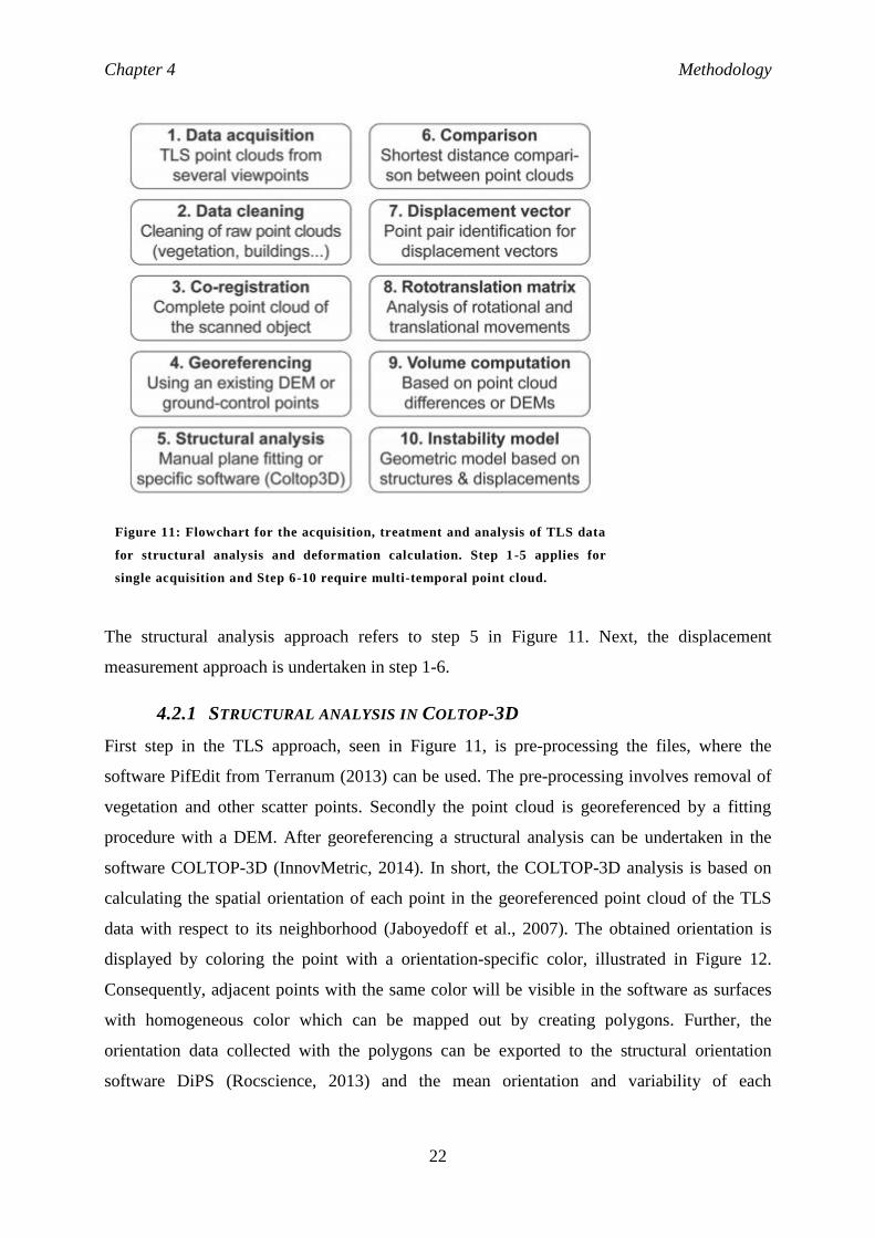
and displacement analyses. Figure 11 presents an overview of the steps involved in this
approach. A brief description of each can be read in e.g. by Oppikofer et al. (2012).
Chapter 4 Methodology
22
The structural analysis approach refers to step 5 in Figure 11. Next, the displacement
measurement approach is undertaken in step 1-6.
4.2.1 STRUCTURAL ANALYSIS IN COLTOP-3D
First step in the TLS approach, seen in Figure 11, is pre-processing the files, where the
software PifEdit from Terranum (2013) can be used. The pre-processing involves removal of
vegetation and other scatter points. Secondly the point cloud is georeferenced by a fitting
procedure with a DEM. After georeferencing a structural analysis can be undertaken in the
software COLTOP-3D (InnovMetric, 2014). In short, the COLTOP-3D analysis is based on
calculating the spatial orientation of each point in the georeferenced point cloud of the TLS
data with respect to its neighborhood (Jaboyedoff et al., 2007). The obtained orientation is
displayed by coloring the point with a orientation-specific color, illustrated in Figure 12.
Consequently, adjacent points with the same color will be visible in the software as surfaces
with homogeneous color which can be mapped out by creating polygons. Further, the
orientation data collected with the polygons can be exported to the structural orientation
software DiPS (Rocscience, 2013) and the mean orientation and variability of each
Figure 11: Flowchart for the acquisition, treatment and analysis of TLS data
for structural analysis and deformation calculation. Step 1 -5 applies for
single acquisition and Step 6-10 require multi-temporal point cloud.

Chapter 4 Methodology
23
discontinuity set is determined. A basic assumption in COLTOP-3D is that topographic
surfaces is considered to reflect the discontinuity sets that exist in the slope.
Due to the high accuracy of the technique, geometrical properties such as persistence and
roughness can also be obtained from the structural analysis in COLTOP-3D. Hence, structural
mapping by TLS data is favorable compared to traditional geological field mapping when the
instability is located in areas that are not easy accessible. Because LiDAR scans cover a larger
section of the slope it provides better mapping of major persistent structures that controls the
large-scale stability of the slope and is an efficient tool for justifying that all major
discontinuity sets have been mapped during the field investigation. Moreover, the information
obtained from TLS-data are more statistically representative, thus it can be used to reduce the
uncertainty of a structural model that are based on field measurements.
As for all analytical tools there are limitations and uncertainties also related to structural
analysis with TLS data. Before applying the obtained results for further analyses it is
necessary to evaluate the realibility. Therefore, results obtained by structural mapping in TLS
Figure 12: COLTOP-3D color scheme. The scheme is a
colored stereonet that is used to represent the spatial
orientation of a point in the DEM point cloud. The color
represent the aspect and the intensity represents the dip
angle (modified from (Hanssen (1998); Jaboyedoff et al.
(2007))).
Chapter 4 Methodology
24
data should whenever possible be justified with results from other investigation techniques.
For an overview of publications that deals with several aspects of the application of TLS to
rock slope assessment, see Abellán et al. (2014)
4.2.2 DISPLACEMENT ANALYSIS IN POLYWORKS
The software Polyworks (Terranum, 2013) can be applied for a deformation analysis of a
rockslide, see e.g.Abellán et al. (2014). The software detects volume changes in the slope by
comparison of temporal TLS-data that are scanned with exactly the same orientation. First
step in the displacement analysis is to combine temporal TLS point cloud models. In the
undertaken study data from 2012 and 2013 were used. This was performed by applying tools
in IMAlign in Polyworks. Further the combined model was imported to IMInspect
(Polyworks), in which the analysis displacement was carried out. A comprehensive
description of the displacement measuring approach can be read in Loftesnes (2010).
In particular, detection of areas with increased rock fall activity is important to detect in a
large rock slope stability analysis, because rock fall areas might reflect zones of higher slope
deformation activity.

Chapter 4 Methodology
25
4.3 Stability analysis
The factors that are considered when choosing an analysis method for a rock slope analysis
are mainly 1) the complexity of the geological conditions 2) time and costs. Stead et al.
(2006) gives recommendations of preferred analysis method based on the complexity of the
geological conditions, which are illustrated and described in Figure 13 and briefly described
in the further text:
I. Kinematic and Limit equilibrium analysis: Before applying numerical modeling a
slope stability problem is usually identified by a kinematic feasibility test. Kinematic
feasibility tests assess the possibilities for different failure mechanisms (planar sliding,
wedge sliding and toppling failure) based on the discontinuity orientations with
respect to the slope orientation. A kinematic feasibility test was undertaken for the
Håkåneset rockslide in the project assignment, and is presented in Chapter 5.4.2.
Figure 13: This figure gives recommendation for preferred slope stability a nalysis
method based on the complexity of the assumed dominant failure mechanism forming a
sliding surface (Stead et al., 2006)
Chapter 4 Methodology
26
When a failure mechanism is defined as kinematically feasible the stability can be
evaluated with limit equilibrium (LE) analysis to determine a factor of safety (FS). LE
is a mathematical method that is time and cost effective and has therefore been an
efficient tool in slope stability analysis for years. However, in order to obtain a
satisfactorily result with LE calcuations, the geology usually have to be oversimplified
by assuming that the failure is translational and involves release on smooth basal, rear
and lateral surfaces where the principle active damage mechanisms are progressive
failure and/or asperity breakdown (Stead et al., 2006).
II. Numerical methods: Numerical modeling in slope stability analysis is use for stress
and deformation calculations (Stead et al., 2006). The fast development of computers
that can handle a large quantity of data has led to the development of numerical
models that can perform calculations on complex models. In rock engineering this
means that essential complexities like geometry, material anisotropy, non-linear
behavior, in situ stresses, the presence of several coupled processes, e.g.: pore
pressures and seismic loading, can be more reliable represented compared to when a
limit equilibrium model is used for stability analysis. This means that the effect of
step-path failure involving internal deformation and fracturing of intact rock can be
taken account of if a numerical modeling is applied in a slope stability anaysis.
Consequently, one of the major advantages with numerical modeling contra limit
equilibrium analysis is that the calculations can be performed without pre-defining
failure planes. As a result, a more reliable estimate can be obtained, however this is
fully dependent on the quality of the input parameters that are used. It is crucial to
remember that numerical analysis basically is about investigating the sensitivity of the
model due to changing input parameters, and should never be interpreted as exact
calculations with definite answers (Nilsen et al., 2000). Numerical modeling is only a
tool that can provide information that helps to understand the conditions in a unstable
rock mass, and the results obtained with the modeling should always be verified with
field observations.
Numerical methods are divided into continuous models and discontinuous models,
where
1. Continuous models consider the material as continuous through the whole
model. Consequently, rock mass behavior is essential in these models, and they
Chapter 4 Methodology
27
are best suited for the analysis of slopes that comprises massive, intact rock,
weak rock and soil-like or heavily jointed rock masses.
2. Discontinuous models dissect the material into blocks that represents
discontinuities. Thus, the representation of discontinuity orientation, location
and behavior become of fundamental importance. Discontinuous models are
favorable to apply in cases where the instability is controlled by discontinuity
behavior.
III. Hybride methods involve analyses where continuum–discontinuum codes with
fracture simulation capabilities are combined. These codes are expensive and slow,
thus mostly used to complex translation/rotational instabilities where failure requires
internal yielding, brittle fracturing and shearing (in addition to strength degradation
along release surfaces).
4.3.1 NUMERICAL MODELING WITH FINITE ELEMENT METHOD (FEM) OF
THE HÅKÅNESET ROCK SLIDE
For the stability assessment of the Håkåneset rockslide it was suggested by the main
supervisor Nilsen (2014) to use the software Phase2, which is a continuous numerical Finite
Element Method (FEM ) including the application of a Shear Strength Reduction (SSR)
method. The main reasons for choosing this method are its applicability and easily available
license at NTNU. This chapter justifies the application of a FEM as a suitable numerical
model for investigating the aims of study of the Håkåneset rockslide.
Finite Element Method (FEM) in general
Finite Element Method (FEM) is a continuous numerical modelling technique that is widely
applied to slope stability analysis. (Hammah et al., 2007). Hammah et al. (2007) lists the
following as the primarily reasons for its popularity:
1. Can handle multiple materials in a single model (material heterogeneity)
2. Readily accommodate non-linear material responses
3. Model complex boundary conditions, and
4. Easily available software

Chapter 4 Methodology
28
Slope failure in FEM is assumed to occur "naturally" through the zones in which the shear
strength of the material is insufficient to resist the shear stresses (Griffiths and Lane, 1999).
This assumption is the basis for defining factor of safety (FS) as (Wyllie and Mah, 2004) :
(Eq. 1)
By this definition FS can be used to reflect a calculated stability of a slope, where FS < 1
indicate unstable slope conditions.
Software: Phase2 (Rocscience)
The two-dimensional software Phase2 (Rocscience, 2014a) is used in this study. Phase
2 is an
efficiently tool for model progressive failure, where the calculation basically involves
determining relative displacements and stress conditions in a slope model. Several analysis
techniques in Phase2 can be applied to investigate these conditions. This study includes a
Groundwater Seepage analysis and a Shear Strength Reduction (SSR) analysis that provides a
FS for the slope model based on defined input parameter values. In addition, maximum shear
strain and displacement contour plots are provided (among others) that can be used for visual
analysis to get an impression of the stability conditions in the slope. Model set up, analysis
settings and input parameters used for the FEM analysis in this study is discussed in Chapter
6.
Groundwater Seepage analysis
A groundwater seepage analysis in Phase2 allow for modeling the pore pressure distribution
and the location of a groundwater table (pore pressure = 0) in the slope model based on
defined hydraulic material parameters (Rocscience, 2014b). The results from the groundwater
analysis are automatically added to the stress analysis. In this way the modeling is performed
with effective stress values. Since there is no information about the location of the
groundwater table in the mountains slope at Håkåneset, this was analysis option was
considered efficient to use.
Chapter 4 Methodology
29
Finite Element Shear Strength Reduction Analysis (FE-SSR)
By the definition of Hammah et al. (2004):
"The Shear Strength Reduction (SSR) technique of a finite element model is a simple slope
stability analysis approach that involves a systematic search for a stress reduction factor
(SRF) or factor of safety (SF) value that brings a slope to the very limits of failure."
As defined by Eq. 1, the factor of safety is defined as the ratio of the actual shear strength to
the minimum shear strength required to prevent failure. Wyllie and Mah (2004) describe a
SSR analysis as a process that basically involves a systematically reduction of the shear
strength until collapse occurs in the model, and the critical stress reduction factor (CSRF) is
the ratio between the rock's actual strength to the reduced shear strength at failure. This
systematically reduction of the shear strength is simulated by running series with an
increasing trial factor of safety, f. If Mohr-Coulomb material is assumed, f determines the
reduction of the actual shear strength properties, cohesion (c) and friction angle (φ) for each
series (Wyllie and Mah, 2004). The trial factor of safety is increased gradually until the slope
fails. At failure, the factor of safety equals the trial factor of safety. At this point the numerical
solution does not converge because equilibrium cannot be established for the stress- and
displacement distribution calculations when the particular simulated material strength are
used as input for the calculations (Griffiths and Lane, 1999).
Parameter study
Due to high uncertainty related to input parameter values for the rock mass, a parameter study
has been performed on assumed critical parameters. This involves a systematic change of the
chosen input parameters to see how it affects the conditions of CSRF, shear strain
concentrations. An overview of all the analyses that has been performed in this study of the
Håkåneset rockslide is presented in Chapter 6.4.
Justification of methods used for Håkåneset study
As defined in the project assignment, does the rock mass at Håkåneset comprise of brittle
metavolcanic rock that is heavily dissected by 5 main discontinuity sets of non-persistent
joints, see Chapter 5. As recommended by Stead et al. (2006), Figure 13, numerical methods
should be applied to model scenarios where the development of a failure plane involves

Chapter 4 Methodology
30
complex translation, meaning that a high degree of asperity breakdown, progressive failure,
fracturing of brittle intact rock are expected. The fact that no failure surface is identified for
the Håkåneset rockslide and the non-persistence of the joints are the reason for interpreting
the geology to be so complex that numerical modeling is chosen over LE for investigating the
stability of this slope. According to Hammah et al. (2007) can the use of FE-SSR analysis on
blocky rock mass failure mechanisms (planar, wedge, toppling) with absolutely no a priori
assumptions on the modes, shapes or locations of these mechanisms be justified if the
material is so evenly jointed that it can be assumed as a continuum. With this basic
assumption, FE-SSR is considered as a suitable to used to predict the development of a failure
plane in the heavily dissected rock masses in the rockslope at Håkåneset.
The Håkåneset rockslide slides into the Lake Tinnsjø, thus hydrogeological conditions are
essential to include in the model in order to get the most realistic model. Simultaneously,
adding the hydrogeological parameters also adds new uncertainties to the model. Because no
groundwater measurement exists for the study area, the automatic groundwater seepage
analysis in Phase2 was chosen as a good approach for including pore pressure calculations in
the slope model.

Chapter 5 Geological investigation
31
5 RESULTS AND FINDINGS FROM GEOLOGICAL
INVESTIGATION OF THE HÅKÅNESET ROCKSLIDE
(INCLUDES RESULTS OBTAINED IN THE PROJECT ASSIGNMENT)
This chapter is a summary of the project assignment Håkåneset, Tinnsjø - Geological
investigation of potentially rockslide performed by the candidate as an introductorily study to
this master thesis. In addition, results from a supplementary thin section analysis performed
during the master thesis are also presented. This chapter gives information about: identified
joint sets, important mapped and interpreted geological features, geotechnical parameters for
the rock mass and the joint surfaces in the study area and the result of a kinematic feasibility
test.
5.1 Rock mass characterization
5.1.1 FIELD OBSERVATIONS
During the field investigation two main rock type units was observed: 1) a dark rock with
quartz, calcite and amphibolites crystallizations of various character, interpreted as a
metaryholitic rock, and 2) a light rock type with visible foliation planes, interpreted as a
gneissic rock. The lithological boundary between these units could not be mapped out as a
distinct boundary. Observations along the road cut gave the impression of dark metarhyolitic
rock at the lowest elevations in the road cut and a transitional transformation to the lighter
rock type further up. Mostly the assumed gneissic bedrock was observed at the locations up
slopes of the road. The most distinct bedrock characteristics are shown in Figure 14.

Chapter 5 Geological investigation
32
5.1.2 THIN SECTION ANALYSIS
Four thin sections were prepared to analyze the texture and mineralogy of the in situ rock.
The in situ rock samples were taken in the road cut close to Location 1 and 2 in Appendix 1.
Thin section #1 is prepared from a rock sample of the light colored rock unit and thin section
#2, # 3 and #4 were prepared from the dark colored rock unit explained in Chapter 5.1.1. Thin
section #1, #2 and #3 were prepared with orientations in order to investigate the presence and
orientation of foliation and possible microfractures. Several photos of the analyzed thin
sections prepared in the laboratory at NTNU can be seen in Figure 15, Figure 16 and Figure
17. All photos are taken with the same settings with plain light (ppl) polarisor crossed (xpl)
and with fluorescence.
Figure 14: Some rock type characteristic observed in the area
during field work. A) Gneissic rock with poorly developed
schistose foliation. B) Metavolcanic ryholite with calcite (white)
and brown FE-mineralized surface. C) Metarhyolite with quartz
and calcite minerals. D) Porous ryholite with re-crystallized
calcite and quartz in the pore holes.

Chapter 5 Geological investigation
33
Mineralogy
All thin sections are dominated by a fine grained matrix of feldspar, quarts, mica and epidote.
Muscovite is identified in thin section #1 (visible as "disco" colored grains in 1_xpl Figure
15b). In thin section #3(Figure 16) and #4 (Figure 17) the fine grained matrix has high biotite
content (brownish color in 3_ppl (Figure 16a) and 4_ppl (Figure 17a)), whereas in section
1_ppl (Figure 15a) the amount of biotite is significantly lower. Also, the fine grained matrix
in all thin sections have mineral grains of oxides (black, non-transparent), calcite (cross-
hatched cleavage pattern), feldspar and quarts that are of bigger size than the matrix itself.
The major dark colored area in section 1_xpl (Figure 15b) is interpreted as a phenocrystal
(Sørensen, 2014).
Texture: deformation and foliation
The texture of the grains is clearly deformed, which can be seen from the rounded shape of
the feldspar grains and the asymmetric shape of the oxides in all thin sections. All thin
sections also show a foliation due to a preferred orientation of deformed mineral grains, and
mica sheets oriented parallel to the deformed grains, se e.g. Figure 16a/b. In #1 (Figure 15)
the oriented mica sheets are manly muscovite, while in #2, #3(Figure 16) and #4 (Figure 17)
there are mainly biotite defining the foliation. The foliation trends NE in #1 and N-S in #3.
Micro fractures
Microfractures are identified in thin section #3 (Figure 16c) and #4a-b (Figure 17 c and f)
(yellow color), developed parallel to the foliation. The microfractures are filled with calcite. It
can be seen that the presence of coarse grains in the fine grained matrix affect the fracture
development by changing its orientation, as can be seen in thin section #4b Figure 17b. In #4a
the interaction between the fracture development and the foliation is clear: the microfractures
appear more scattered within the biotite layer which illustrates the weakening effect of
foliations.

Chapter 5 Geological investigation
34
Interpretations
The following interpretations are made based on the thin section analysis of the rock at
material from Håkåneset:
- The difference between the light colored and dark colored rock units observed in field
is due to variable biotite content. However, since the texture is the same it is
considered reasonable that for further stability analysis a homogeneous rock type can
be assumed.
- The presence of phenocrystals confirms that the rock mass is of magmatic origin
(Sørensen, 2014).
- The rounded and asymmetric shaped feldspar and oxide grains may in addition to the
dominance of fine grained matrix be interpreted as an evidence that the rock mass has
undergone significant deformation (Sørensen, 2014). This justifies that the rock has
undergone shear deformation and metamorphism.
- The rock is clearly foliated due to deformed grains and mica sheets oriented parallel to
the deformed grains. The foliation appears with N-NE trend. Hence, significant
strength anisotropy in the rock is expected.
- Microfractures development is disturbed by the presence of coarser mineral in the fine
grained matrix.
- The microfractures are developed approximately parallel to the foliation.

Chapter 5 Geological investigation
35
-
a)
b)
Oriented (North up )thin section a) 1_ppl and b) 1_xpl. Presence of the former
phenocrystals (major dark feature in 1-xpl) as pyroclasts confirms that the rock is of
volcanic origin. Deformed grains and muscovite sheets oriented in a preferred orietation
trending NE defines the foliation in the rock. The in situ rock appears with a light color
due to low biotite content.
Figure 15: Oriented (North up) thin section #1 of the light colored in situ rock type within the
Håkåneset instability.

Chapter 5 Geological investigation
36
a)
b)
c)
a) Thin section 3_ppl, b) 3_xpl and
c)3_fluorocence image. High biotite
content give the in situ rock a dark color.
Rounded and deformed grains oriented
~N-S defines a foliation orientaion.
Branched microfracture partly developed
parallel to the preferred foliation
direction.
Figure 16: Oriented (North up) thin section #3 prepared from the dark colored situ rock within
the Håkåneset instability.

Chapter 5 Geological investigation
37
a) ppl
d) ppl
b) xpl
e) xpl
c) fluorized
f) fluorized
Photos from thin section #4. Biotite sheets are oriented parallel to the preferred direction of
deformed grains in the fine grained matrix. How the foliation contols the development of
microfractures is cleary observed in the c). Also note how fractures are deflected around large
quartz aggregates in d).
Figure 17: Thin section #4 (not oriented) of dark colored in situ rock sample within the
Håkåneset instability.

Chapter 5 Geological investigation
38
5.2 Rock mass and discontinuity parameters
5.2.1 JUSTIFICATION OF ASSUMED HOMOGENEOUS MATERIAL TYPE
The rock mass in the unstable rock slope at Håkåneset comprises a metavolcanic rock that
appears both as light and dark colored units. There are not observed any distinct lithological
boundary between these units. Thin section analysis of in situ rock samples revealed that the
rock mass of both units have the same texture. In general both units have high mica content;
however in the light colored rock muscovite is dominant, while biotite dominates in the dark
colored rock, thus being an explanation to the color difference. The mica sheets are oriented
parallel to a preferred direction of deformed grains, giving the rock strong anisotropic
character due to foliation. For anisotropic rock material will the strength estimates obtained
by uniaxial compressive strength test be highly dependent on the load direction relative to the
anisotropy. However, the anisotropy of the in situ rock material from Håkåneset was not taken
into account in the laboratory work conducted in this study, and therefore it was evaluated
that calculating the mean of all obtained test, independent on rock unit, would be the best
approach to obtain a representative estimate for the rock strength. The lack of lithological
boundary in field, same texture in all thin sections, and insufficient shear strength parameters
to distinguish between the light and dark rock units are all factors that justifies that for a
stability model the rock mass in the rock slope at Håkåneset can be considered as anisotropic
homogeneous metavolcanic rock.
5.2.2 ROCK MASS PROPERTIES
Geotechnical properties
Deformability parameters (E, ν), unconfined compressive strength (UCS) and basic friction
angle (φb) are necessary input parameters in the numerical modelling approach (Wyllie and
Mah, 2004). These parameters were determined by laboratory tests on cores of rock material
collected from the Håkåneset site during the project assignment. All tests were performed at
the Geological Engineering Laboratory of NTNU/SINTEF, Trondheim, Norway, following
the standard of ISRM (2007) and Barton-Bandis standard procedures described in (Grøneng
and Nilsen, 2009). The test results are given in Table 4.

Chapter 5 Geological investigation
39
Reliability of the laboratory estimates
Estimation of rock mass parameter can be challenging and involves several uncertainties
regarding both the representativeness of the tested material and the laboratory approach. For
the values for the in situ rock from Håkåneset provided in Table 4, the following comments
are considered as important:
The rock samples used for the testing was partly detached and taken from the road cut,
which imply that it can be strongly affected by the road construction.
The rock material is strongly anisotropic due to foliation, thus the loading direction is
essential in the compressive strength test. Because the foliation was difficult to
recognize on the rock samples, the loading direction relative to the foliation is not
Table 4: Geotechnical data (mean values and standard deviation) of rock materoal taken
from the site of Håkåneset rock slide. Blue numbers represent the number of tested
specimens.
Rock sample location
Rock type E [GPa]
(#)
(#)
γ [kN/m3]
UCS [MPa]
(#)
Failure angle*
(#)
Tilt angle [φb] (#)
Weakness zone (J1-fault)
Meta- volcanic
45,6 ± 4,6 (6)
0,21 ± 0,013
(6)
30 81,3 ± 22,6
(3)
23 ± 6 (3)
27,7 ± 2,2 (2)
Possible rupture surface (J1 surface)
Meta- volcanic
33,1 ± 3,3 (3)
0,13 ± 0,006
(3)
30 59,5 ± 4,6 (3)
29 ± 1 (1)
27,3 ± 1,7 (1)
Road cut Meta- volcanic
54,4 ± 4,3 (3)
0,18 ± 0,030
(3)
30 154,3 ± 29,4
(2)
18 ± 3 (2)
28,4 ± 1,2
(1)
Average mean
44,3 0,17 30 98,4 23 27,8
#: number of tested specimens * Measured on the failed specimens from uniaxial compressive strength test

Chapter 5 Geological investigation
40
uniform for the tested samples. This will be a significant bias in the obtained strength
estimates for the rock material.
Even though the specimens seemed to have different character (described in the
project assignment) the material is assumed homogenous.
Geological strength index (GSI)
The geotechnical rock properties presented in Table 4 are values measured for intact rock
conditions. However, the actual rock mass in nature is highly disturbed and dissected by
discontinuities, which implies a significant reduction in the strength of the geological unit.
The Geological Strength Index (GSI) provides a number which, when combined with the
intact rock properties, can be used for estimating the reduction in rock mass strength for
different geological conditions (Hoek, 2007). The in situ rock mass at Håkåneset is blocky,
where four joint sets are dominant. The joint surfaces conditions are: slightly weathered, Fe-
mineralization, planar, undulating rough (see Table 6, Chapter 5.2.2), which is best classified
as good "Good" surface conditions, as defined in Hoek (2007) and will indicate a GSI value
of the range 60 to 80, see Appendix 3. At some localities the surface conditions were
smoother and better described as "Fair", implying a GSI value of 40 to 60.
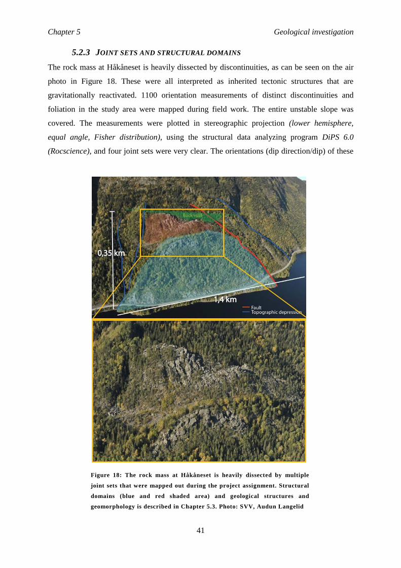
Chapter 5 Geological investigation
41
5.2.3 JOINT SETS AND STRUCTURAL DOMAINS
The rock mass at Håkåneset is heavily dissected by discontinuities, as can be seen on the air
photo in Figure 18. These were all interpreted as inherited tectonic structures that are
gravitationally reactivated. 1100 orientation measurements of distinct discontinuities and
foliation in the study area were mapped during field work. The entire unstable slope was
covered. The measurements were plotted in stereographic projection (lower hemisphere,
equal angle, Fisher distribution), using the structural data analyzing program DiPS 6.0
(Rocscience), and four joint sets were very clear. The orientations (dip direction/dip) of these
Figure 18: The rock mass at Håkåneset is heavily dissected by multiple
joint sets that were mapped out during the project assignment. Structural
domains (blue and red shaded area) and geological structures and
geomorphology is described in Chapter 5.3. Photo: SVV, Audun Langelid

Chapter 5 Geological investigation
42
were determined by cluster analysis, which involve defining windows around the pole
clusters. The contour range was set to 2-10 for this analysis. The joint sets are labeled as J1,
JF2, JF3 and J4 (corresponding to J1, J2, J3 and J4 in the project assignment). Additionally, a
less distinct and more variable oriented foliation and coincident foliation planes were
recognized and referred to as schistose foliation, SF. Further, the measurements were
organized and plotted as steronets for 20 localities on a base map of the study area (Appendix
1). Even though the measurements are very consistent, a systematic change in the orientation
of joint set J1 and J4 was identified. Together with mapped major tectonic features (described
in Chapter 5.3), this systematic change was the basis for dividing the study site in three
subaerial domains, see Figure 19. Dip and dip direction of the joint sets for each domain are
given in Table 5, and visualized in Appendix 4. All joint sets are mapped in all domains.
However, some joint sets were not statistically significant with the chosen criteria for the
cluster analysis (contour range 2-10). In these cases the contour range was increased to 1-10,
and the set window was drawn based on this for the particular joint set cluster. Joint set
orientations that are determined with an increased contour range are written with grey color
and italicized style in Table 5. The joint set characteristics based on the field observations are
briefly summarized in Table 6.

Chapter 5 Geological investigation
43
Table 5: Mean dip and dip direction (Fisher distribution) of identified joint sets given for the
whole study area (ALL) and for each defined subdomain (N orth, Lower-South, Upper-South).
Joint set orientations in black are determined with a contour range of 2 -10 in DiPS (Rocscience).
Grey colored and italicized style represent orientations where the contour range was increased to
1-10 in order make the joint set statistically significant.
Joint set
Discontinuity type Average all domains
(DipDir/Dip)
Domain North (DipDir/Dip)
Domain Lower-South
(DipDir/Dip)
Domain Upper-South
(DipDir/Dip)
J1 Exfoliation 074°/59° ± 20° 071°/62° ± 16° 076°/51° ± 19° 075°/63° ± 14°
JF2 Fault plane (conjugate) 358°/65° ± 18° 359°/69° ± 18° 355°/51° ± 14° 360°/67° ± 16°
JF3 Fault plane (conjugate) 133°/77° ± 20° 137°/72° ± 14° 138°/79° ± 14° 140°/78° ± 8°
J4 Joint 208°/76° ± 16° 237°/62° ± 13° 213°/76° ± 10° 207°/71° ± 15°
SF Schistose foliation 237°/19° ± 21° 284°/11° ± 16° 031°/16° ± 14° 277°/15° ± 18°
Figure 19: Defined structural domains for the study area: Subaerial domains are called North (N),
Upper-South (U-S) and Lower-South (L-S), and are based on a systematic spatial variability in
discontinuity orientations. Subaqueous domains are Bathymetric-North (B-N) and Bathymetric-South (B-
S) and are divided based on geomorphological features that are visible on bathymetric images.
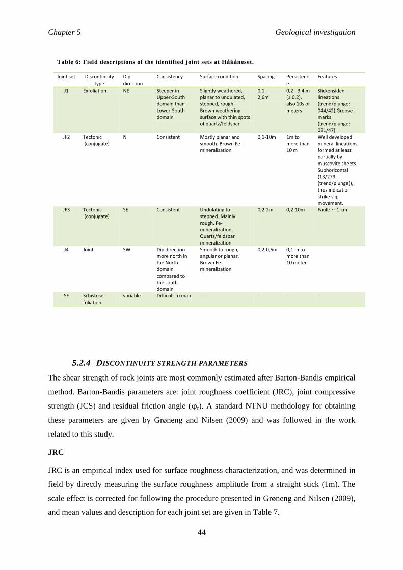
Chapter 5 Geological investigation
44
5.2.4 DISCONTINUITY STRENGTH PARAMETERS
The shear strength of rock joints are most commonly estimated after Barton-Bandis empirical
method. Barton-Bandis parameters are: joint roughness coefficient (JRC), joint compressive
strength (JCS) and residual friction angle (φr). A standard NTNU methdology for obtaining
these parameters are given by Grøneng and Nilsen (2009) and was followed in the work
related to this study.
JRC
JRC is an empirical index used for surface roughness characterization, and was determined in
field by directly measuring the surface roughness amplitude from a straight stick (1m). The
scale effect is corrected for following the procedure presented in Grøneng and Nilsen (2009),
and mean values and description for each joint set are given in Table 7.
Table 6: Field descriptions of the identified joint sets at Håkåneset.
Joint set Discontinuity type
Dip direction
Consistency Surface condition Spacing Persistence
Features
J1 Exfoliation NE Steeper in Upper-South domain than Lower-South domain
Slightly weathered, planar to undulated, stepped, rough. Brown weathering surface with thin spots of quartz/feldspar
0,1 - 2,6m
0,2 - 3,4 m (± 0,2), also 10s of meters
Slickensided lineations (trend/plunge: 044/42) Groove marks (trend/plunge: 081/47)
JF2 Tectonic (conjugate)
N Consistent Mostly planar and smooth. Brown Fe-mineralization
0,1-10m 1m to more than 10 m
Well developed mineral lineations formed at least partially by muscovite sheets. Subhorizontal (13/279 (trend/plunge)), thus indication strike slip movement.
JF3 Tectonic (conjugate)
SE Consistent Undulating to stepped. Mainly rough. Fe-mineralization. Quarts/feldspar mineralization
0,2-2m
0,2-10m
Fault: ~ 1 km
J4 Joint SW Dip direction more north in the North domain compared to the south domain
Smooth to rough, angular or planar. Brown Fe-mineralization
0,2-0,5m 0,1 m to more than 10 meter
SF Schistose foliation
variable Difficult to map - - - -

Chapter 5 Geological investigation
45
JCS
JSC is an index that represents the strength of the rock at the discontinuity surface. JCS was
estimated by applying Schmidt hammer test on three natural, weathered surfaces, following
the procedure in Grøneng and Nilsen (2009). The Schmidt hammer values were converted to
representative JCS values that are presented in Table 8 below. According to Grøneng and
Nilsen (2009) can JCS be assumed equal to the unconfined compressive strength (UCS, σc) of
the intact rock if the joints are completely unweathered. In reality natural joint surfaces will
always be weathered to some extent, and JCS will be lower than UCS tested on specimens in
laboratory. UCS estimate of the intact rock from Håkåneset determined in the laboratory was
in the range 60-154MPa (Table 4), whereas mean JCS values ranges from 120-223MPa
(Table 8). Due to the fact that JSC values obtained with Schmidt hammer is greater than the
UCS values determined in the laboratory on intact rock, the Schmidt hammer results has been
considered not reliable. The unrealistic correlation may also be explained with the fact that
some specimens was loaded subperpendicular to the foliation, thus a low value is obtained.
It was decided to use the laboratory estimate as input value for further investigations, as this
will give the most conservative result.. A widely accepted estimate for JCS on weathered
joints based on laboratory rock strength estimates are 1/4 σc, recommended by Barton and
Choubey (1977). With a mean value for USC of 98MPa for the tested Håkåneset rock mass,
25MPa is assumed as an acceptable input JSC value for the natural joints in the study area.
Basic friction angle (φb) and residual friction angle (φr)
By the definition in Grøneng and Nilsen (2009) can the basic friction angle (φb) be considered
as a material constant and refers to smooth, planar surfaces in fresh rock. The residual friction
angle (φr) refers to the residual condition of natural joint surfaces after shear displacement.
Empirical formulas have been developed for determining φr from φb. In this study φb was
determined with tilt test in the laboratory, after the recommendations in Grøneng and Nilsen
(2009). Four specimens were tested, and the tilt angle was assumed to be a representative
value for φb, as justified in (Grøneng and Nilsen, 2009). The results of the tilt test are given in
Table 4. According to Barton (1973) can φr for natural joints be assumed equal the φb for
sawn surfaces (the tilt angle) of the same rock material, and is usually in the range between
25° and 35°. This assumption is used for the discontinuities in the Håkåneset rock mass, thus
φr = φb = 28° is assumed as representative value.

Chapter 5 Geological investigation
46
Table 7: Estimated JRC for the defined joint sets. Estimated after a standard NTNU
methodology presented by Grøneng and Nilsen (2009)
Joint set JRC Description Source
J1 13,7 ± 4,7 planar to undulated, stepped, rough
Field estimate
JF2 4,7 ± 1,5 planar, smouth Field estimate
JF3 > 20 rough, undulating Field estimate
J4 9,5 ± 2,1 smooth to rough, angular or planar
Field estimate
SF 5 ± 1 smooth, stepped Chart value
Table 8: Estimated JCS (USC) for natural discontinuity surfaces at the Håkåneset site obtained
with Schmidt hammer as presented in Grøneng and Nilsen (2009). Suggested empirical estimate
calculated from UCS obtained in the laboratory
Joint set Assumed geological feature Rock type JCS (MPa) Source
J1 Back scarp Granitic 195 ± 60 Field work
J1 Sliding plane Metarhyolitic 120 ± 32 Field work
JF3 Weakness zone Metarhyolitic 223 ± 27 Field work
1/4σc Laboratory speciemens Granitic/metarhyolitic ~25 Empirical formula by Barton and Choubey (1977)

Chapter 5 Geological investigation
47
Estimated discontinuity shear strength of J1
Determinations of the shear strength of discontinuities, that are assumed to be important
sliding surfaces, are essential in a slope stability analysis (Grøneng and Nilsen, 2009).
Grøneng and Nilsen (2009) assumes that the shear strength of a discontinuity is defined by
four geological properties: 1) the surface roughness, 2) the strength of rock at the
discontinuity surface, 3) the normal stress acting on the discontinuity and 4) the amount of
shear displacement. These are represented by three index parameters; the joint roughness
coefficient, JRC , the joint wall compressive strength, JCS, and the residual friction angle, φr,
in addition to the normal stress, σn, action on the surface. Figure 20 gives the relationship
between shear strength and normal stress on a representative J1 surface within the study area.
This relationship is calculated after a modified Coulomb criteria after the procedure given by
Grøneng and Nilsen (2009). The non-linear relationship between peak shear strength and
normal stress for low stress levels is justified in for instance Nilsen et al. (2000)An average
value of the estimated JCS given in Table 8 for J1 is used in the calculation.
Figure 20: Estimated joint shear strength for the Håkåneset slope. The estimation is performed after
the empirical method of Barton-Bandis, described in Grøneng and Nilsen (2009). Input values found
in Table 4, Table 7 and Table 8
0
0,5
1
1,5
2
0 0,5 1 1,5 2 2,5 3 3,5
Shea
r st
ress
, τ [
MP
a]
Normal stress, σ [MPa]
Joint shear strength of surface Estimated after Barton-Bandis empirical method

Chapter 5 Geological investigation
48
5.3 Major geomorphological features
Several geomorphological features could be mapped on both air photos and in the field, and
these are assumed to affect and control the stability of the slope. These features are outlined in
Figure 21. A brief description of these structures is given in the following text. A more
detailed description can be read in the project assignment
Subaerial features
J1-fault zone: A weakness zone (red dotted line) in Figure 21 is recorded to daylighting in the
road cut in the north domain (Location 6 in Appendix 1). The width is estimated to be 8,0 m.
The weakness zone material consists of highly fractured rock mass with lense structures and
fine grained joint filling down to clay size (fault breccia) and high mica content. Estimated
GSI value is 27-50. The material characteristic indicates that the damage is a result of tectonic
activity. The tectonic activity interpretation is supported by observations of mineral lineations
(13/279) on a JF2 (63/007) surface within the weakness zone material and slicken sides
(42/044) at a J1 (53/077) surface below the weakness zone. The same J1 surface have groove
Figure 21: Important geomorphological features that are assumed to be affecting and
controlling the stability of the slope. The three defined structural domains are highlighted
and arrows show the direction of the measured movement in the slope by dGNSS (not in
scale).

Chapter 5 Geological investigation
49
marks (47/081) (not statistically significant), that is interpreted as evidence of gravitationally
reactivation of the fault. On air photos the weakness zone seems to continue as a NNW-SSE
trending depression, defining the boundary between the U-S and L-S domains in Figure 19
(yellow line in Figure 21). i.e. congruent with the orientation of joint set J1.
Back scarp: The upper limit of the instability is defined by a back scarp at an elevation of
approximately 550 m a.s.l. The orientation of this steeply dipping wall is 65/070 (±06/±012)
(calculated from 18 measurements), thus it is parallel to J1 surfaces.
JF3-fault zone: A distinct SW-NW trending fault zone (red solid line) is interpreted as the
northern limit of the instability. This linear feature is also clear on the bathymetric map (see
Figure 21), and continues down to approximately 300 meters depth. Based on field
measurements the orientation of the fault is 78/314, thus congruent with joint set JF3.
Subaquatic features
Spatially variable bedrock structures: The bathymetric map reveals that subaquatic a
southern area with significantly bedrock structures can be seen relative to a northern area
where the bedrock surfaces appear smoother, see Figure 21. This is the reason for dividing the
submerged slope in a northern and a southern domain. The bedrock structures in the southern
domain are prominent in the north and less distinct in the south.
Multiple sliding planes: Several linear SE-NW trending features of 40 - 100 m length can be
seen in the prominent subaquatic bedrock structures at 200 - 300 meters depth (purple lines in
Figure 21). In the far north of the southern domain two SW-NE trending steps are observed.
These linear features and steps are interpreted as an indication that multiple sliding planes
exists in the slowly deforming rock mass.
Buttress: South in the southern domain is a dome like feature. This feature stands out from a
typical glacial eroded valley profile, and is therefore assumed to be a buttress of hard rock that
was resistant to the glacial erosion in (see Figure 21).

Chapter 5 Geological investigation
50
5.4 Preliminary findings
5.4.1 LATERAL LIMITS OF THE ROCKSLIDE
The lateral limits of the instability have been determined by geomorphological mapping and
interpretation of aerial photos and bathymetric images. The surface area has been calculated
to be 0,50 km2 subaerial and 0,54km
2 subaqueous by the 3D Analyst tool in ArcMap (ArcGiS,
ESRI).
Two distinct faults striking SW-NE parallel to joint set J3 form the northern lateral release
surface. Such a clear release surface does not occur in the south and the bathymetric data
rather suggest that the limit of the unstable area in the south is transitional.
5.4.2 RESULTS OF KINEMATIC FEASIBILITY TEST
Based on the geological investigation of the Håkåneset the instability was concluded to be
structurally controlled by the discontinuities. In the project assignment a kinematic feasibility
test was performed for each of the subaerial domains, testing for the possibility of planar
sliding, wedge failure and block toppling. The test was performed under the criteria in NGU's
hazard analysis published by Hermanns et al. (2012b). Maximum slope inclination
determined in ArcMap 10.1 (Esri, 2012) is assumed. The results are illustrated by Figure 22.
For detailed description about how to interpret the plots, see Hermanns et al. (2012b).

Chapter 5 Geological investigation
51
a)
b)
c)
Figure 22: Kinematic feasibility test results for a) Lower-South (L-S) domain. b) Upper-South (U-
S) domain. c) North (N) domain. The feasibility for planar, wedge and toppling failure are tested
assuming maximum slope inclination. Guidelines given for the risk and hazard classification syst em
provided by NGU (Hermanns et al., 2012b)are followed.

Chapter 5 Geological investigation
52
Based on the interpretation of the kinematic feasibility test in Figure 22 there are five
important failure mechanisms that are considered as relevant for the further stability analysis
of the Håkåneset rock slide:
1. Planar sliding is feasible in steep parts of the slope along planes of minimum dipping
values of an exfoliation plane (J1) dipping 40-80 degree in NE direction towards
Tinnsjø.
2. Either steeply dipping J1 surfaces like along the back scarp, or joint set (J4) dipping
40-90 degree into the slope, can form rear release surfaces.
3. Bi-planar sliding is feasible along a compound sliding surface defined by the
exfoliation J1 and the variable schistose, SF.
4. Wedge sliding formed by the intersection of the conjugate joint sets J2 and J3 is
feasible where the slope is steeper than 50-60 degrees.
5. Toppling of small rock volumes. (Not important for a massive failure of the slope.)

Chapter 6 FEM model setup
53
6 THE FEM MODEL USED FOR THE HÅKÅNESET
ROCKSLIDE
This chapter presents all settings and input parameters which serves as a basis for the stability
analysis of the Håkåneset rockslide undertaken in this study. It gives all the information that
should be known before interpreting (Chapter 7).
The stability analysis performed in this study is undertaken by applying the numerical
modeling software Phase2 (Rocscience, 2014a). A description of this software and reason for
choosing it for the slope stability of the Håkåneset rockslide is discussed in more detail in
Chapter 4.5.1. This chapter first verifies the construction of a representative model for the
studied slope, presented in Chapter 6.1. The chosen analysis settings are presented in Chapter
6.2. Chapter 6.3 presents the structure of the parameter study undertaken in the following
analysis, and lists the different slope models that have been analyzed. The discussion for
choosing input rock mass parameter values are summarized in Chapter 6.4.
6.1 Model geometry set up
The numerical modeling in this study is carried out on a 2-dimentional one stage model. The
model is constructed based on a scaled cross section profile of the Håkåneset rock slope. The
profile was extracted from a 1m resolution DEM in ArcMap 10.1 (Esri, 2012) using the 3D
Analyst tool. The location of the profile is through the central part of the study area,
illustrated in Figure 23 as a red line. This location is chosen to include the assumed most
active part of the slope with respect to slope deformation. The assumption about increased
activity in the north of the study area is based on an interpretation of bedrock structures on
bathymetric images, where pronounced structures appear in the central part of the study area,
as described in Chapter 3.2. The profile is oriented perpendicular to the valley slope and rises
from the bottom of the lake at 300 meters depth in Lake Tinnsjø and up to the mountain
plateau at 962 m.a.s.l. In addition, it has been essential to have a favorable orientation of the
profile with respect to mapped structural and geomorphological features that are assumed as
controlling factors for the slope stability. Thus, the profile intersects with the exfoliation joint
set J1, the prominent SW-NE striking JF3-failt fault system and the NW-SE striking J1-fault
cutting through the slope. The characterization of these geomorphological features can be read
in Chapter 5.3.

Chapter 6 FEM model setup
54
Boundary conditions
The geometry of the model is constructed on the basis of recommendations given in Wyllie
and Mah (2004), see Figure 24, in order to avoid boundary effects. Boundary effects in this
matter are related to the artificial boundaries of the model, i.e. far-field boundaries that do not
correspond to natural ground surface boundares. In reality no artificial boundaries exist, thus
they may influence the analysis results if they are located to close to the area representing the
slope stability problem in the model. In any numerical model for slope stability analysis the
condition of the artificial boundaries must be specified either as prescribed displacement or as
prescribed stress. Prescribed displacement are most commonly used for slope stability
problems (Wyllie and Mah, 2004), therefore also applied in this study. Table 9 gives an
overview of the displacement boundary set up of Håkåneset rockslide model.
Figure 23: AA' is the trend of the cross section profile
used to construct the Phase2 model. Profile
constructed from 1m resolution DEM in Esri (2012)
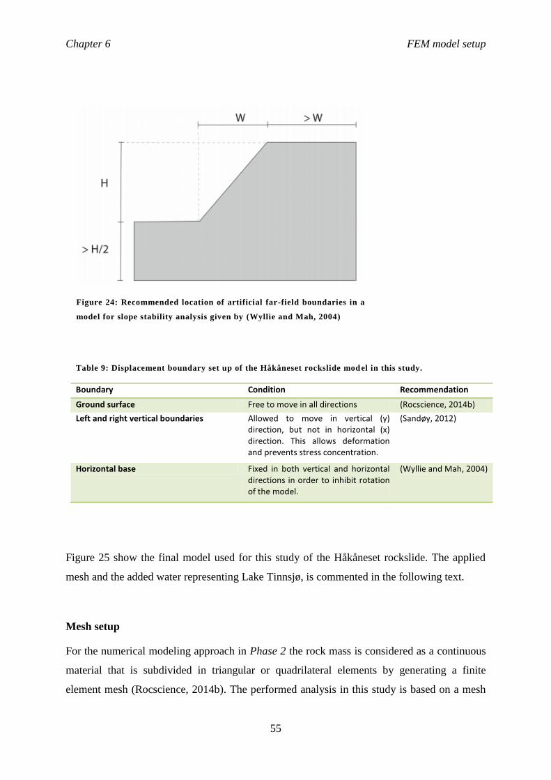
Chapter 6 FEM model setup
55
Figure 25 show the final model used for this study of the Håkåneset rockslide. The applied
mesh and the added water representing Lake Tinnsjø, is commented in the following text.
Mesh setup
For the numerical modeling approach in Phase 2 the rock mass is considered as a continuous
material that is subdivided in triangular or quadrilateral elements by generating a finite
element mesh (Rocscience, 2014b). The performed analysis in this study is based on a mesh
Figure 24: Recommended location of artificial far-field boundaries in a
model for slope stability analysis given by (Wyllie and Mah, 2004)
Table 9: Displacement boundary set up of the Håkåneset rockslide model in this study.
Boundary Condition Recommendation
Ground surface Free to move in all directions (Rocscience, 2014b)
Left and right vertical boundaries Allowed to move in vertical (y) direction, but not in horizontal (x) direction. This allows deformation and prevents stress concentration.
(Sandøy, 2012)
Horizontal base Fixed in both vertical and horizontal directions in order to inhibit rotation of the model.
(Wyllie and Mah, 2004)

Chapter 6 FEM model setup
56
of 3-noded triangular elements, following recommendation given by Trinh (2014). This mesh
set up gives a fast modeling but still with a satisfactorily quality of the computation. A
"Graded" mesh is used, by recommendation given in Rocscience (2014b).
The size of the elements or the density of the mesh in the model is determined by applying the
Advanced Mesh Region option under the Mesh Setup option in Phase2. By defining a mesh
region it is possible to construct a more time effective model where the mesh has a higher
density in the interesting part of the model, i.e. around the unstable slope, and lower density
mesh in the parts that are not close to the unstable slope region. The mesh region was
assigned to the model of this study within the same area that is defined as a SSR Search Area
(see Shear Strength Reduction analysis set up in Chapter 7. 2) in Figure 25. The density of the
mesh is determined by defining an element length of 75 m, which means that the length
between the elements at the model boundary within the region (corresponding to the slope
face at this model) is 75 m. The mesh type within the region was chosen as Uniform, because
this gives an uniformly meshed rock mass over the instability of the study and the quality of
the calculations are equal for all depths in the slope model. This is considered to give the most
representative analysis in the search for a feasible sliding plane.
Outside the defined mesh region, a graded mesh type was chosen. When using Advanced
Mesh Region the Default Number of Nodes on External is not affecting the meshing of the
model. However, the mesh is dependent on the Gradiation factor of the graded mesh outside
the mesh region, as this factor determine the discretization of all boundaries outside the
defined mesh region. A Gradiation factor of 0,1 (default) is used for this model. With this, the
model has a generated mesh with 994 elements and 534 nodes, which is assumed to be a
satisfactorily mesh quality for this study (confirmed by Trinh (2014)).
Pounded lake water
The unstable slope at Håkåneset has both a subaerial and a subaquatic component, thus the
Lake Tinnsjø should be included in the model to make it as close to the reality as possible. In
a Phase2 model the effect of a lake can be investigated by constructing a "pounded water" in
the model (Rocscience, 2014a). Rocscience (2014b) defines pounded water as water which is
impounded against a dam or a slope, and is represented as a blue hatch pattern above the
ground surface, as shown in Figure 25a,b). The pounded water conditions are assigned to the
model by defining the Set Boundary Conditions under the Groundwater option, as described

Chapter 6 FEM model setup
57
in tutorials given by Rocscience (2014b). The boundary type Total Head are used, which
require input on the elevation of the phreatic surface at the external boundaries. Since the
surface elevation of the Lake Tinnsjø is 191 m.a.s.l., a Total Head Value of 191m was
assigned to the right external boundary from the lower right corner and up to the level of 191
m in the model, thus representing the elevation of the assumed phreatic surface. Selection
mode was defined as Boundary Segments.
Pounded water applies an additional stress to the slope due to the weight of the water
(Rocscience, 2014b). However, the Total Head Boundary Conditions described above do not
define the weight of the pounded water. Therefore, the weight of the pounded water must be
defined by adding a Pounded Water distributed load to the model. The pounded water load is
found under the Loading option in Phase2. The water is modeled as an equivalent distributed
load, and is represented as blue arrows in the model in Figure 25a). A pounded water load,
also with a Total Head Value corresponding to the elevation of the lake surface at 191 m.a.s.l,
was defined.

Chapter 6 FEM model setup
58
a)
b)
Figure 25: The Phase2 model used for the stability analysis of the Håkåneset rockslide. The profile is
constructed from the AA' profile in Figure 23

Chapter 6 FEM model setup
59
6.2 Analysis set up
General settings
For the numerical modeling in this study a plane strain analysis with Gaussian solver type is
defined, as recommended by Rocscience (2014b).
Stress analysis set up
For the Stress Analysis set up the following settings are defined:
Maximum Number of
Iterations
The default number of 500 was used.
Tolerance: The tolerance of a model imply the point at which the
calculations of the analysis should be considered as
converged (Rocscience, 2014b). The stresses in the
analyses of this study are simulated with a tolerance of
0.001, which is the default value in Phase2.
Number of Load Steps: Auto (default)
Convergence type: The convergence type defines the stopping criteria for the
calculations. The default Absolute Energy is used as
convergence criteria in this study.
Tensile failure reduces shear
strength to residual.
This option was chosen because it implies that if tensile
failure occurs at a point in a material (and shear failure has
not already occurred), the shear strength of the material at
that point will be automatically reduced to the residual
shear strength parameters for that material. Rocscience
(2014b) recommends this as a realistic assumption to make,
particularly for brittle materials, thus it is considered as a
representative condition for the metavolcanic rock masses
Chapter 6 FEM model setup
60
at Håkåneset. When defining this criterion it is required that
the material is defined as plastic.
Joint tension reduces joint
stiffness by a factor of 0,01
(default value):
This setting specify how the joint property stiffness is
reduced if the joint element is subjected to tensile stress
normal to the joint. The rock mass at Håkåneset is highly
dissected by closed and open joints, and therefore it was
considered that this condition is essential to include in the
model.
Use effective stress analysis: Since the lake water and consequently groundwater is
assumed as an essential part of the Håkåneset model, it is
found reasonable to define that the analysis should be based
on effective stresses in the slope. By the description given
in Rocscience (2014b) this means that calculated
deformation is a result of changes in effective stress due to
pore pressure changes, assuming that changes in
deformation or loading do not affect the pore pressure.
Groundwater seepage analysis set up
Due to lack of groundwater level measurements, it was decided to define a steady-state finite
element ground water seepage analysis to be included in the modeling. To perform a
groundwater seepage analysis the Total Head boundary conditions must be set to define the
hydraulic boundary conditions of the model. For the Håkåneset model this corresponds to the
elevation of the water level in the lake for the right boundary segments, which was already
defined when constructing the lake in the model (see Chapter 6.1. Pounded water). By
studying air photos it can be observed that several small lakes that do not have any open
drainage channels, are located at the plateau above the unstable area. This observation can be
interpreted as an indication that the water table in the slope is close to the surface at high
elevations. Therefore, hydraulic conditions with a total head value of 962m, were assigned to
all segments at the left vertical boundary of the model. The chosen value corresponds to the

Chapter 6 FEM model setup
61
elevation of the mountain at the left end point of the profile from which the model was
constructed.
For simplification has infiltration conditions not been taken into account in the analysis of this
study and boundary conditions at the free surface representing the mountain slope was
assigned as Unknown (P=0, Q=0).
Since the hydrogeological conditions in the rock slope in this study are unknown, it must be
emphasized that the groundwater seepage settings adds significant uncertainties to the model.
A parameter study on the groundwater conditions will therefore be important to perform.
Shear Strength Reduction (SSR) analysis setup
The SSR analysis was defined with the default settings of "Initial Estimate of SRF" = 1 and
"Tolerance"=0.001.
A SSR area is defined including the region where the slope is located, visible as a dotted
square. Within the SSR-area the material is considered as brittle, and outside the area it
behaves elastically (Rocscience, 2014b).
6.3 Input parameters for the Håkåneset rock mass
A slope stability analysis is undertaken in order to predict where the rock mass is most likely
to fail based on the input parameters, i.e. the aim is to search for a feasible failure surface
within the rock mass in the model. In most cases of large scale rock slope failures is the
development of a failure surface not a uniform process, but rather a complex deformation in a
combination of unfilled joints (rock-to-rock contacts), filled joints (gouge material) and
bridges of intact rock (Grøneng et al., 2009). This is also assumed to be the case for the
Håkåneset rockslide, which comprises a heavily jointed rock mass made up of hard brittle
blocks separated by non-persistent discontinuity surfaces. The strength of such rock masses
depends on the strength and deformability of the intact pieces and on their freedom of
movement which, in turn, depends on the number, orientation, spacing and shear strength of
the discontinuities (Hoek, 1983).
In Phase2 a representative rock masses quality is assigned to the model by 1) defining
materials with estimated parameters 2) defining joints with estimated properties. Estimation
of material parameters for the rock mass at Håkåneset are discussed in Chapter 6.3.2 and
estimated discontinuity properties are discussed Chapter 6.3.3.

Chapter 6 FEM model setup
62
6.3.1 MATERIAL MODEL AND STRENGTH CRITERION OF JOINTED ROCK MASS
A numerical model requires input parameters related to rock mass behavior and strength
parameters. Necessary input parameters depend on what material model and strength criteria
that are assumed to describe the rock mass.
Material models
Material models are idealized stress/strain relations that describes how the material behaves
under variable stress conditions. Figure 26 is an illustration the different material models that
are common to consider.
The elastic behavior of the material up to the level of failure (peak strength) is described by
assuming a failure criterion. Failure criterions are discussed in the next section. The different
material models describe how the strength of the material is assumed to change after the point
of failure. The residual strength relative to the peak strength describes the plastic strain-
softening model of the material due to failure.
Figure 26: Stress-strain relations that represent the behavior of the rock mass
when different material models are assumed. The residual strength relative to
the peak strength describes the plastic strain-softening model of the material
(ed. Hoek (2007)).

Chapter 6 FEM model setup
63
Failure criterions
Mohr-Coulomb strength criterion
Mohr-Coulomb strength criterion is a traditional failure criterion, where the shear strength of
a rock is represented by a linear relationship between the normal stress state, n, and the
material properties cohesion (c) and inner friction angle () after the definition e.g. found in
Hoek (2007):
(Eq. 2)
Hoek-Brown empirical strength criterion
The mechanics behind a large landslide is complex because the rock mass failure is controlled
by the characteristics of both intact rock material and discontinuities (Stead and Eberhardt,
2013). Due to this complexity, the failure in rock masses has a non-linear character that
cannot be described with the linear Mohr-Coulomb criterion. Therefore, in order to describe
the non-linear behavior of blocky rock masses, the empirical failure criterion Generalized
Hoek-Brown was developed (Hoek et al., 2002).
The Generalized Hoek-Brown failure criterion for jointed rock mass is an empirical failure
criterion that is defined by (Hoek, 2007):
(Eq. 3)
where:
σ1' and σ3' are the maximum and minimum effective principal stresses at failure,
mb is the value of a Hoek-Brown constant mi for the rock mass:
(Eq. 4)
s and a are constants which depend upon the rock mass characteristics
(Eq. 5)
(Eq. 6)

Chapter 6 FEM model setup
64
and σci is the uniaxial compressive strength of the intact rock pieces.
The factors mb, s and a are included to reduce the properties of intact rock so that a strength
estimate for jointed rock mass is obtained. These reducing factors are calculated on the basis
of two factors that express the characteristic of joints in the rock mass and the rock mass
quality:
- Geological Strength Index (GSI) of the rock mass.
- Disturbance factor D, depending upon the degree of disturbance due to blast damage
and stress relaxation. D varies from 0 for undisturbed in situ rock to 1 for disturbed
rock mass.
With this, Hoek-Brown is commonly used to describe the strength of jointed rock masses
(Hoek and Brown, 1997). However, this criterion also assumes isotropic rock conditions and
rock mass behavior. Therefore, it should only be used for rock mass which are dissected by a
sufficient number of closely spaced discontinuities with similar surface conditions, so that
isotropic behavior involving failure on discontinuities can be assumed. For the same reason,
this criterion can only be applied when the block sizes are small compared to the overall
object being studied (Hoek, 2007). With these restrictions, the Generalized Hoek-Brown
strength criterion is favorable for describing the failure of big slopes with jointed rock masses
like at Håkåneset
Equivalent Mohr-Coulomb parameters
Equivalent Mohr-Coulomb parameters are estimates for the shear strength parameters
cohesive strength, c', and the angle of friction, φ', and is obtained by converting Hoek-Brown
parameters to traditional Mohr-Coulomb parameters over a specified stress range (Hoek et al.,
2002). This is a commonly used approach because even though Hoek-Brown failure criterion
is assumed to best describe a jointed rock mass, most geotechnical software is still written in
terms of the Mohr-Coulomb failure criterion (Hoek et al., 2002). As for finite element
computation, finding estimates for the Hoek-Brown parameters require calculations that slow
down the analysis considerably (Hammah et al., 2004). Therefore, it is favorable to use the
equivalent Mohr-Coulomb parameters as input parameters in a numerical modeling. The
conversion of the parameters can be undertaken with the software RocLab provided by

Chapter 6 FEM model setup
65
(Rocscience, 2011). Equivalent Mohr-Coulomb parameters have been used as in put
parameters in his study.
6.3.2 MATERIAL PARAMETERS
With the assumption of the rock mass as homogeneous, a single material model was
constructed. Required parameters are properties that are related to unit weight of the rock and
its strength and elastic properties. The results of field and laboratory test of rock samples from
the particular study area (Chapter 5) supplemented empirical values and recommendations
from Rocscience (2014b) have been used to obtain required Equivalent Mohr-Coulomb input
values for the SSR-analysis in Phase2.
Equivalent Mohr-Coulomb strength parameters was converted from the following Hoek-
Brown parameters (Hoek et al., 2002) in RocLab (Rocscience, 2011):
- Uniaxial compressive strength (σci) of intact rock.
- Value of Hoek-Brown constant for intact rock (mi).
- Geological Strength Index value (GSI-value) for the rock mass.
- Disturbance factor D.
- Deformation modulus of the intact rock, E
Chosen values for the estimation are discussed below. Input and output of the conversion is
summarized in Table 10
sigci (σci) The uniaxial compressive strength of intact rock has been tested by uniaxial
compressive strength test on specimens (d = 50 mm) that were cored from rock
samples collected from the weakness zone, the possible rupture surface and
from rock of good quality within the limits of the unstable rock masses in the
study area. The rock sample from the weakness zone was taken from rock of the
best quality within the zone. The laboratory work was undertaken and described
in the project assignment, and the test results are summarized in Table 4 in
Chapter 5. Due to the uncertainties related the obtained laboratory estimates (see
Chapter 5) it was considered that an average value of all test results would be
the most representative estimate for the uniaxial strength of the overall rock
mass. Thus, the value of 98MPa for σci was used as input in the estimation in

Chapter 6 FEM model setup
66
RocLab.
GSI During the field investigation the rock mass was given a GSI value of 60-80 for
rough surfaces and 40-60 for smoother surfaces, see Chapter 5.2.2 and
Appendix3. Based on this, a GSI value of 60 chosen as a representative input
value for average rock mass.
mi This parameter was not tested during the laboratory work related to this study.
Therefore, the guidelines given by Hoek (2007) have been the basis for
assessing a representative value. Rocscience (2011) recommends a mi in the
range 25±5 for a rhyolitic rock and 28±5 for a gneissic rock. Therefore, the
value 27 is chosen as a representative value for the rock masses at Håkåneset in
this study.
D According to Rocscience (2011) the disturbance factor should not be applied to
the entire rock mass. In a natural rock slope, the GSI value take account for the
disturbance due to fracturing and weathering of the rock mass. Therefore, after
discussion with the supervisor, a disturbance factor D = 0 was chosen for this
modeling.
Ei For the same reason that an average value of all valid tests was used to find an
estimate of σci, the average value of the performed deformability tests was used
to find an estimate for Young's Modulus, Ei. The average of 12 deformability
tests is 44300MPa.
From the Hoek-Brown input parameters discussed above, the equivalent Mohr-Coulomb
strength parameters cohesion, c, and friction angel, φ, are calculated. The strength of a
material depends on the stress conditions, as can be read from the definition of shear strength
in Eq. 2 (Hoek and Brown, 1997). Thus, the apparent cohesion and apparent friction angle
have to be determined by taking the normal stress σn acting on the sliding surface into
account. However, the software used in this study require a constant input value of c and φ,
which means it is necessary to first determine a assumed normal stress level for the material
where a feasible failure surface is expected to form. The normal stress can be estimated from
the overburden to a possible sliding plane, by the relation
Chapter 6 FEM model setup
67
Eq. 7
The major advantage by applying the FE-SSR technique in this study was that no prior
assumption about a failure surface was needed. However, the normal stress dependent shear
strength parameters bring up a limitation of the method if σn have to be calculated from the
overburden of a feasible sliding surface that has to be assumed before the analysis. This
highlights the importance of performing a parameter study of the shear strength parameters
when investigating the slope stability. Based on the field observations the orientation of the
J1-fault (described in Chapter 5.3) would a logical feature to use for determining a normal
stress level that can be used to obtain a initial estimates for the materiel shear strength
parameters. The calculation of the normal stress level is given in Appendix 5. Overburden
ranges from 0 to approximately 75 m in the subaerial part of the slope and increases to
approximately 200m at the level of the lake floor. 100 m overburden was chosen as a
reasonable mean value. Further, the normal stress was calculated as an average normal stress
according to the weight component of an overburden of h=100m acting perpendicularly on
the sliding plane with an average dip angle of 46° and a specific rock density of 30kN/m3
(Table 4) after Equation 6. The input values give a normal stress of 2,1MPa. The effective
normal stress value is obtained taking the pore pressure acting on the plane into account. For
simplification and for considering a worst case scenario with fully saturated slope materials,
an average groundwater height of 100 m was assumed, resulting in an effective normal stress
of σn=1.4 MPa. (Hydrostatic stress calculated to be 0,7MPa). The equivalent M-C parameters
under a normal stress condition of 1.4 MPa can be determined by the Instantaneous MC
sampler in RocLab, see Appendix 6. The results of the rock mass strength parameter
estimations in RocLab are given in Table 10.

Chapter 6 FEM model setup
68
Dilation angle
The shearing of rock induces a volume increase due to normal displacement in the rock
(Rocscience, 2014b). Dilation angle increases with the rock shear strength, and ranges from
zero to φ. According to Hammah et al. (2008) , the dilation angle does not have significant
influence in the slope stability problems due to general low confinement stresses. Also for the
rock mass at Håkåneset the confinement stress can be expected to be low, as the heavily
dissected rock at the surface indicates significant stress relief have taken place. Based on this,
dilation angle is set to zero in the undertaken modeling.
Table 10: Estimated material properties of the rock mass at Håkåneset. Conversion of Hoek-Brown
parameters to equivalent Mohr-Coulomb parameters obtained in RocLab. M-C parameters are used as input
in the Phase2 model.
INPUT (RocLab) Parameters:
Symbol Mean Value
- 30% +30% Source
Strength criterion: Generalized Hoek-Brown
Uniaxial compressive strength intact rock (UCS)
ci [MPa] 98 67 127 Laboratory work undertaken in the project assignment
Geological Strength Index GSI 60 42 78 Field observations during the project assignment work
Intact rock parameter mi 27 19 35 Evaluated based on inbuilt RocData values in RocLab
Disturbance factor D 0 0 0 Discussed with main supervisor Bjørn Nilsen
Young's Modulus Ei [MPa] 44300 30100 57590 Laboratory work undertaken in the project assignment
Unit weight [MN/m3] 0,03 0,03 0,03 Laboratory work undertaken in the project assignment
OUTPUT (used as input in Phase2 models) Strength criterion: Mohr-Coulomb
Parameters: Initial
(σn =1,4MPa)
30 % reduced strength parameter input
(σn =1,4MPa)
30% increased strength parameter input
(σn =1,4MPa)
Håkåneset model Model 1 Model 2 Model 3
Peak cohesion Cpeak [MPa] 1,5 0,8 3,6 RocLab estimation
Residual cohesion Cres [MPa] 1,0 0,5 2,4 Assumed 2/3 of peak
Peak friction angle peak [°] 63 54 68 RocLab estimation
Residual friction angle res [°] 42 36 45 Assumed 2/3 of peak
Defomation modolus Em [MPa] 23036 5507 49357 RocLab estimation
Peak tensile strength
σt (peak)[MPa] 0,2 0,04 0,7 RocLab estimation
Residual tensile strength
σt (res)[MPa] 0,1 0,03 0,5 Assumed 2/3 of peak

Chapter 6 FEM model setup
69
Tensile strength
Tensile strength reflects the interlocking of the rock particles when they are not free to
dilate (Hoek and Brown, 1997). According to Stead and Eberhardt (2013) can tension
cracking be interpreted as an early sign of instability. Consequently, the tensile strength is an
essential parameter for slope stability. The applied tensile strength estimate in this study is
obtained from the RocLab calculation of equivalent Mohr-Coulomb parameters (Table 10).
Material type: Elastic and plastic
Required strength properties of a material in the Phase2 model depend on whether the material
is assumed as elastic or plastic. In order to perform a SSR-analysis the material has to be
defined as plastic. A plastic strain-softening model is assumed for this study, and input of a
residual strength of the material is required. By discussion and recommendation from Trinh
(2014), the residual values are calculated as 2/3 of the peak values. This is considered as an
reasonable estimate for the relative rough surfaces observed in field at Håkåneset.
Table 11: Initial input material properties used for the SSR analysis in Phase 2
Parameter Source
Elastic type Isotropic
Unit weight [MN/m3] 0,03 Laboratory test in project assignment
Poisson's ratio 0,18 Laboratory test in project assignment
Youngs modulus (rock mass) Em [MPa] 23036 RocLab estimation
Peak cohesion at 1,4MPa c' [MPa] (peak) 1,5 RocLab estimation
Residual cohesion at 1,4MPa c' [MPa] (resid) 1,0 (Trinh, 2014)
Peak friction angle at 1,4Mpa (peak) 63 RocLab estimation
Residual friction angle at 1,4Mpa (resid) 42 (Trinh, 2014)
Peak tensile strength t'[MPa] (peak) 0,2 RocLab estimation
Residuak tensile strength t'[MPa] (resid) 0,1 RocLab estimation
Dilation angle d 0 (Hammah et al., 2008)

Chapter 6 FEM model setup
70
6.3.3 DISCONTINUITY PARAMETERS
Barton-Bandis discontinuity shear strength parameters
When a rock mass is dominated by joints with no filling, the shear strength of the joint surface
is critical for the stability due to the rock-to-rock contact (Wyllie and Mah, 2004). The
frictional force at the joint surface depends on 1) the surface roughness, 2) the strength of
rock at the discontinuity surface, 3) the normal stress acting on the discontinuity and 4) the
amount of shear displacement (Grøneng and Nilsen, 2009). Barton and Choubey (1977)
relates these properties to the three indices: joint roughness coefficient, JRC , the joint wall
compressive strength, JCS, and the residual friction angle, φr, in addition to the normal stress,
σn, action on the surface. The definition of the shear strength (τ) with the Barton-Bandis
parameters is:
(Eq. 8)
Barton-Bandis parameters for the rock mass at Håkåneset were obtained in the project
assignment, following the methodology given by Grøneng and Nilsen (2009). Estimated JRC
for the joint sets is given in Table 7, and JCS values are given in Table 8. Realistically will
the strength of discontinuities be significantly lower than for intact rock. However, the
Schmidthammer test results (Table 8) indicated significantly higher values for JCS, than
respective USC values determined in the laboratory. Therefore, the Schmidt hammer values
were considered as not reliable, and the empirical estimate of 25 MPa as a value for JCS have
been used in the modeling (see Chapter 5.2.2.). As justified by Grøneng and Nilsen (2009)
can φr be assumed equal the basic frictional angle φb determined by tilt test, thus the mean tilt
test value of 28° (Table 4) was used.
In case of slip due to indicated development of a failure surface in the model, the joint shear
strength parameters JRC and JCS will automatically be set to zero and the shear strength will
depend only on the residual friction angle and the normal stress by to the following relation
(Rocscience, 2014b):
(Eq. 9)
When using Barton-Bandis slip criteria for a SSR analysis, the strength reduction is only
applied to the material strength properties while the joints will retain their original strength
properties during the SSR analysis.

Chapter 6 FEM model setup
71
Joint stiffness
Goodman et al. (1968) introduced normal stiffness (Kn) and shear stiffness (Ks) as two vital
parameters that describes joint deformability by relating the normal and shear stress on the
joint element to the normal and shear displacement. Joint stiffness is a parameter that is not
well known and difficult to measure, and several methods for obtaining representative
estimates have been developed. One of these are empirical formulas that estimates the joint
stiffness based on the rock mass properties rock mass E-modulus (Em), intact rock E-modulus
(Ei), rock mass shear modulus (Gm), intact rock shear modulus (Gi) and joint spacing (L).
The calculations are based on the assumption that that the deformability of the rock mass is
due to the deformability of the intact rock and the deformability of the joints in the rock mass.
The formulas are derived based on the average spacing of the joint set, assuming that the joint
orientation is perpendicular to the loading.
In the project assignment it was concluded that development of a failure surface along the
foliation joint set SF should be investigated more in detail by the numerical modeling.
Therefore, a sensitivity test on the joint stiffness of SF is undertaken, based on the values
given in Table 13. The stiffness values are calculated by varying the mean spacing. Brideau et
al. (2008) justifies that importance of schistose foliation in the development of a basal failure
surface, therefore the chosen spacings used to obtain the stiffness estimates can be assumed
realistic.
Table 12: Estimated joint stiffness for each joint set. See Appendix 7a).
Joint set values
J1 JF2 JF3 J4 SF
Normal stiffness Kn [MPa/m] 47992 9598 47992 159972 479917
Shear stiffness Ks [MPa/m] 20335 4067 20335 67785 203355
Table 13: Input for parameters study of joint stiffness of foliation joint set SF. See
Appendix 7
PARAMETER STUDY SF
Average spacing L [m] 0,01 0,1 1 10
Normal stiffness Kn [MPa/m] 4799167 479917 47992 4799
Shear stiffness Ks [MPa/m] 2033545 203355 20335 2034

Chapter 6 FEM model setup
72
Justification of the stiffness parameters
An overview of empirical joint stiffness estimates is given in Sandøy (2012),
Appendix 7b), suggesting that Kn is in the range 3000-10000 and Ks is in the range of
900-1000. The stiffness estimates for the Håkåneset joints are 10.000-500.000 for Kn
and 5000-20.000 (Table 12) for Ks, thus significantly higher than the empirical date
presented by Sandøy (2012)
The estimates obtained for the joint sets at Håkåneset is significantly higher than
Sandøy (2012). The high stiffness calculated for the Håkåneset rock mass was found
to be sensitive to the GSI value, as GSI is critical parameter for the ratio between Ei
and Em. Bandis et al. (1983) gives five factors which is expected to influence the
normal stiffness of joints:
i. initial actual contact area, relative amplitude and vertical distribution of the
aperture between joint wall;
ii. joint wall roughness, expecting that the small scale roughness is the most
critical in controlling normal stiffness;
iii. strength and deformability of asperities;
iv. thickness, type and physical properties of the infilling material.
i., ii. and iv. are factors that are taken account of by the GSI when using estimating Em
based on the generalized Hoek-Brown failure criterion, which supports the assumption
of GSI being the critical factor of the joint stiffness. Because of all uncertainties
related to the calculations of stiffness in general, thus adding significant uncertainties
to the background of the available empirical data, it was decided not to adjust the
stiffness values obtained for the Håkåneset rock mass to the empirical data (after
discussion with Nilsen (2014)).
Addition pressure inside joints
The groundwater pore pressure option is selected as an additional water pressure inside
joints, and the model will take account for the water pressure within the joint due to
groundwater in the joint analysis. This additional pressure is applied to both sides of the joint
wall.

Chapter 6 FEM model setup
73
Initial joint deformation
Initial joint deformation refers to how the joint behaves in regard to the far field stresses
(Rocscience, 2014b). This option is left on so that the joints in the model will deform based
on both the defined far field stresses and the induced stresses due to external water load. As a
result, the stress field in the vicinity of the joints will be altered from the initial far field
distribution, which is assumed to give the most realistic conditions in the model.
Persistent structures: J1-Fault, JF3-fault and back scarp
The AA' profile (Figure 23) intersects with the prominent SW-NE trending JF3-fault, see
Figure 21 (red line), which is interpreted to be a controlling factor for the slope stability by
defining the northern lateral limit. Therefore, this structure is essential to include in the Phase2
modeling. There have not been undertaken any test for obtaining material or discontinuity
strength parameters specific for this fault zone. However, the geological investigation in the
project assignment revealed that the fault zone is developed parallel to the defined JF3 joint
set. Therefore, the JF3-fault has been added to the model as a continuous joint with JF3 joints
properties. This is assumed as a valid simplification because field mapping indicate that there
are no clear difference in the bedrock or surface characteristics in the fault zone relative to the
overall rock mass in the slope. However, the fact that the JF3-fault can be mapped out on
airphoto and DEM and in the field with a persistent ~km, while the JF3 joints only have
persistence in the meter scale imply that there realistically are strength differences.
A second fault, J1-fault (see Chapter 5.3, Figure 21 and Figure 23) intersects with the AA'
profile, and has orientation as suggesting it is developed along J1 joints. The thickness of this
zone is estimated to be ~8m, comprising significantly damaged material and possible clay
content. Because no exact testing has been undertaken on this weakness zone material for
determining its shear strength, it was considered as a reliable simplification to define the J1-
fault as a persistent J1 joint based on the accuracy of the undertaken model. A graph showing
the estimated relation between J1 strength and the normal stress acting on the surface was
obtained in the project assignment and given in Figure 20 in this thesis.
The profile also intersects with a back scarp, see Figure 21 (green line) and Figure 23. The
orientation is measured to be congruent with the J1-fault set, and therefore added to the model
as a persistent J1-fault.

Chapter 6 FEM model setup
74
The chosen values for the necessarily in put parameters in the Phase2 model are summarized
in Table 14:
Ubiquitous joint model
"Ubiquitous joints" is an option in the Interpret mode in Phase2 that display the regions in the
model where the stresses generated from the SSR-analysis are sufficient to cause slip on a
anticipated planes with a user defined orientation (Rocscience, 2014a). Hench, it is an
efficient post-processing tool to investigate if failure can occur on a joint surface when only
its estimated surface shear strength is known. It is fundamental to ubiquitous joints that the
joints themselves do not influence the stress/displacement field. Based on experiences in
Böhme et al. (2013) the introduction of ubiquitous joints in the strength factor calculations
may lead to results that can help to explain the present days morphology. Because J1 and SF
are the joint sets that are assumed to be most critical for the slope stability, these were
included as ubiquitous joints with the properties given in Table 15.
Table 14: Initial joint strength input parameters for the Phase 2 modeling.
Parameter Symbol Joint set values Source
J1 JF2 JF3 J4 SF
Barton-Bandis parameters
JRS 14 5 20 10 5 Field estimate
JCS 25 25 25 25 25 1/4c (Barton and Choubey, 1977)
Basic friction angle
φb [°] 28 28 28 28 28 Tilt test project assignement
Residual friction angle
φr [°] 28 28 28 28 28 φr = φb
(Barton, 1973)
Joint stiffness Normal stiffness Kn [MPa/m] 47992 9598 47992 159972 479917 Formulas given in
Rocscience (2014a)
Shear stiffness Ks [MPa/m] 20335 4067 20335 67785 203355 Formulas given in Rocscience (2014a)

Chapter 6 FEM model setup
75
Joint network model
The rock mass at Håkåneset is observed as highly dissected and blocky, and the instability is
assumed to be structurally controlled. Because of the non-persistency of the identified joint
sets described in Chapter 5.2.2, a joint network models for each set was constructed which
make it possible to construct the joints with orientation, spacing and persistence. In this way
the model reflects realistic conditions by having sections that represent intact rock bridges.
Several scenarios were analyzed by investigating different combinations of joint set in the
model, i.e. different joint networks were assigned to the model. The different models are
presented in Chapter 6.4.
Parallel Deterministic joint networks have been used in this study. This network model is
defined by parallel joints with assumed constant spacing, length and persistence. This is a
simplification of the reality as natural variation in joint orientation and extend are
considerable. However, using the mean orientations as constant values is considered to be
sufficient for the numerical modeling in order to get an impression of the stability of the
slope.
Table 15: Ubiquitous joint Barton-Bandis properties for J1 and SF. Used in Analysis 1.2
Joint set
J1
Joint set
SF
Source
Friction
angle
28 28 Tilt test 5samples in project assignment
Inclination -59 -19 Average all slope measurements from field investigation in
project assignment
JRC 14 5 J1: Direct roughness measurement in field
SF: Chart in Grøneng and Nilsen (2009)
JCS 25 25 1/4 σc recommended from Barton and Choubey (1977)

Chapter 6 FEM model setup
76
Orientation
When constructing the joint networks the joint were defined with 3-dimentional orientation:
dip and dip direction. Values are given in Table 5, which are the orientations obtained from
the field measurements in the project assignment.
A 3-dimentional input requires a definition of a so called Trace Plane. A Trace Plane is the
cross-sectional plane of the Phase2 model, i.e. a vertically dipping plane. Its orientation is by
definition given as the dip direction of this vertically dipping plane, where the dip direction is
given by the normal vector (pointing into the screen) of the trace plane, measured clockwise
from north (Rocscience, 2014b). When the trace plane orientation is entered in the model
Phase2 uses the 3-dimensional input to determine the 2-dimensional traces of the joint planes
on the trace plane. Thus, when a trace plane is defined in the analysis it is not necessary to
transform the measured joint orientations to apparent orientation relative to the model profile.
The trend of the AA' profile, Figure 23, is 078. The AA' trend was determined from the DEM
in ArcMap 10.1 (Esri, 2012). This gives a trace plane orientation of 348.
Spacing
Spacing is the perpendicular distance between the parallel joint planes. Since a trace plane is
defined in the model of this study, then spacing value to enter is the actual, 3-dimensional
spacing between the joint planes. This will be the true perpendicular distance between the
parallel joint planes, i.e. the spacing after the correction of the orientation of the scan line.
Table 6 gives values for true spacing of the joint sets identified at Håkåneset. In order to
simplify the modeling the spacing values was exaggerated. Input values that are used as initial
values are given in Table 16.

Chapter 6 FEM model setup
77
Length and persistence
Discontinuous joints in a joint network in Phase2 are described with persistence and length.
Persistence defines the length of intact material between adjacent joint segments (Rocscience,
2014b). It is important to have in mind that the definition of persistence in Phase2 as given in
(Rocscience, 2014a) differs from the definition used during the geological mapping. The field
investigation used the definition for persistence given by Wyllie and Mah (2004)m, where
persistence is defined as the continuous length or area of the discontinuity, thus corresponding
to the parameter defined as "length" in Rocscience (2014b). As illustrated in Figure 27 the
persistence in the Phase2 model is a measure of joint continuity represented as the ratio of
joint length (L1) to total length along the joint planes (L2), thus having a value between 0 and
1. Input values in the model are given in Table 16.
Since the rock masses at Håkåneset is observed as highly dissected, where air photos indicate
continuous joints of 10s of meters, see photo in Figure 18, a persistence value of 0.7 is chosen
as representative for joint set J1, JF2, JF3 and J4, see Table 16. The schistose foliation is
mapped out as less pronounced. Therefore a persistence value of 0,2 is considered as a
representative average values. With this the model assumes that a significant have to be
damaged in order to develop a failure surface.
The length defines the length of each individual joint in the network, as measured in the plane
of the model (i.e. the trace plane). Input values for length are given in Table 16 based on the
mapped persistence values given in Table 6.
Figure 27: Length (L1) and persistence(L1/L2) of a
joint after the definition used in the Phase2 model
(Rocscience, 2014b).

Chapter 6 FEM model setup
78
Joint end condition
When a joint or joint set is added to the model, the end condition of the joint is specified as
"open" or "closed". For the model of this study the end of the joints are defined as "Closed"
where the joint terminates within the rock mass, and "Open" where the joint boundary
terminates at the free ground surface. A "Closed" joint end condition means that relative
movement (sliding or opening) cannot occur at the joint end, while "Open" joint end condition
means that relative movement in the joint end is allowed. It is relistic that joints can open at
the free surface. Down in the ground on the other hand, joints cannot open without inducing
stresses in the surrendering, which is realistically represented with a "closed" end condition.
Summary of structural discontinuity parameters
In Table 16 the structural input parameters that have been discussed are summarized. These
parameters are used to define the joint network properties for the different models uses for the
stability analysis in Phase2.
Table 16: Chosen discontinuity input values in the Phase2 model. Spacing and length are
exaggerated in order to exaggerate the modeling.
Joint model Parallel Deterministic
Trace plane orientation
348
Joint set Domain Lower-South (DipDir/Dip)
Domain Upper-South (DipDir/Dip)
Spacing Length Persistence* Joint end condition
J1 076°/51° ± 19° 075°/63° ± 14° 30 m 100 m 0,7 Open at boundary,
material and surface contact
JF2 355°/51° ± 14° 360°/67° ± 16° 60 m 100 m 0,7
JF3 138°/79° ± 14° 140°/78° ± 8° 30 m 50 m 0,7
J4 213°/76° ± 10° 207°/71° ± 15° 30 m 100 m 0,7
SF 031°/16° ± 14° 277°/15° ± 18° 100 m 10 m 0,2
* Determined after the definition in Rocscience (2014a) (different than the definition used in field for the
field measurements in Chapter 5. In Table 6 persistence is defined as in Wyllie and Mah (2004)).

Chapter 6 FEM model setup
79
6.3.4 STRESSES
Strength properties depend on the stress conditions (Hoek, 2007). In Phase2 this is taken into
account by defining a stress field. For surface models like a slope model a Gravity stress field
is recommended (Rocscience, 2014a) to represent the in-situ stress conditions. Under this
setting the stress are assumed to vary with depth. The depth was defined to be measured from
the Actual ground surface of the model, which means that the initial vertical stress component
at a given point is calculated using this measured depth and the actual unit weight of the
overlying materials. The unit weight is defined in the Define Material Properties dialog. To
use Actual Ground Surface is favorable for a slope stability study since the ground profile has
a variable elevation. In addition, it is recommended by Rocscience (2014b) to use the Actual
Ground Surface option when performing a SSR-analysis because experiences imply that it
provides more reliable and accurate results with less computation, due to the more realistic
estimate of the initial stress distribution.
The horizontal components of the gravitational field stress are given as Horizontal / Vertical
stress ratios based on the vertical stress at any point in the model. On In-Plane and one Out-
Of-Plane ratio is defined based on the directions of the mean principal stresses used for the
calculations.
Eq. 9
Eq. 10
Input values used for the estimation of the stress field at Håkåneset are based on values found
in a database presented by (Hanssen, 1998). This is known as the last known data set of field
stress measurements for Norway. The data set is a collection of data that is based on available
information on three-dimensional rock stress measurements in NTH (NTNU) and SINTEF
archives, dated from its initial development to 1992. Two boreholes in Rjukan, located 15,5
km west of the study site at Tinnsjø, can be used to get an impression of the field stresses in
the region. Both have a quality ranking B (scale A-D) that should imply representative values.
Note, near surface effects considerably affect the horizontal- and vertical stress components
and lead to relative high compressive or occasionally tensile horizontal stresses at shallow
depths (Hanssen, 1998). Data from Rjukan is given in Table 17 below:
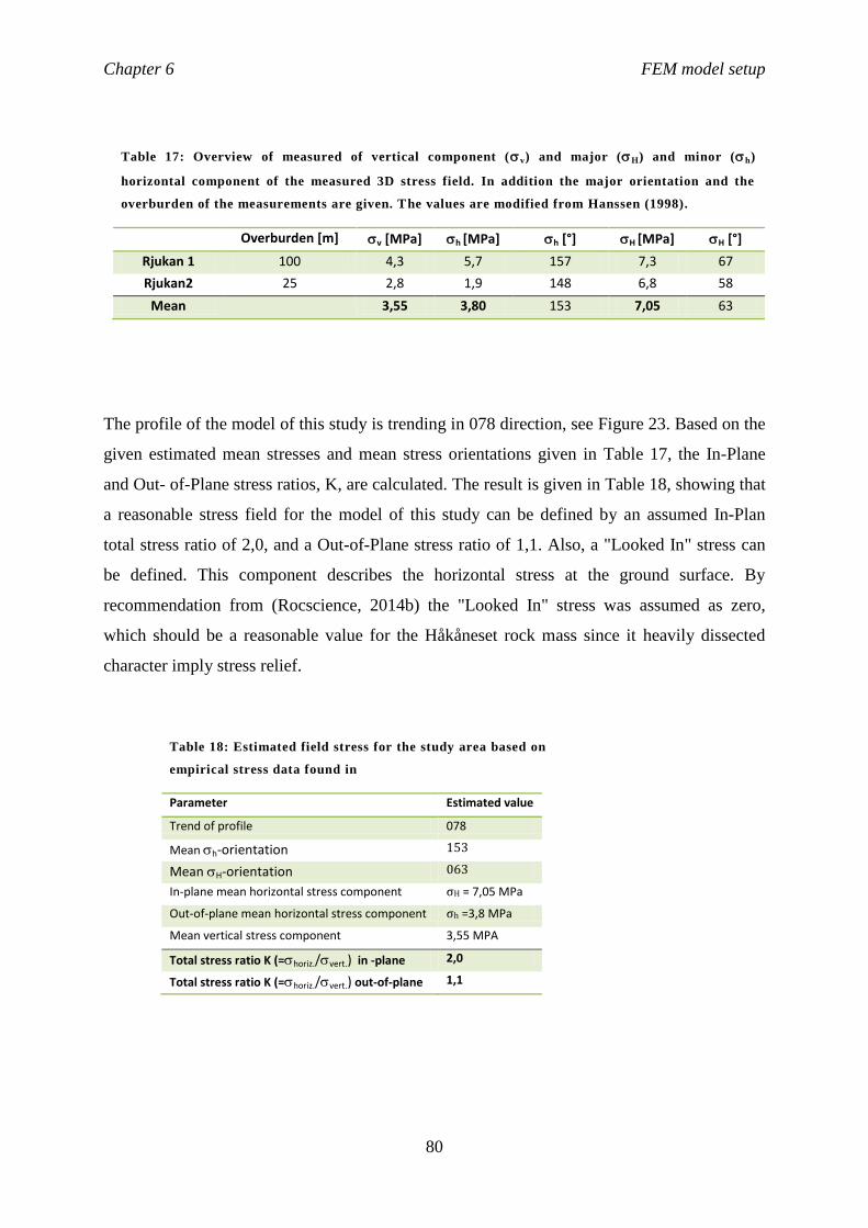
Chapter 6 FEM model setup
80
The profile of the model of this study is trending in 078 direction, see Figure 23. Based on the
given estimated mean stresses and mean stress orientations given in Table 17, the In-Plane
and Out- of-Plane stress ratios, K, are calculated. The result is given in Table 18, showing that
a reasonable stress field for the model of this study can be defined by an assumed In-Plan
total stress ratio of 2,0, and a Out-of-Plane stress ratio of 1,1. Also, a "Looked In" stress can
be defined. This component describes the horizontal stress at the ground surface. By
recommendation from (Rocscience, 2014b) the "Looked In" stress was assumed as zero,
which should be a reasonable value for the Håkåneset rock mass since it heavily dissected
character imply stress relief.
Table 18: Estimated field stress for the study area based on
empirical stress data found in
Parameter Estimated value
Trend of profile 078
Mean h-orientation 153
Mean H-orientation 063
In-plane mean horizontal stress component σH = 7,05 MPa
Out-of-plane mean horizontal stress component σh =3,8 MPa
Mean vertical stress component 3,55 MPA
Total stress ratio K (=horiz./vert.) in -plane 2,0
Total stress ratio K (=horiz./vert.) out-of-plane 1,1
Table 17: Overview of measured of vertical component (v) and major (H) and minor (h)
horizontal component of the measured 3D stress field. In addition the major orientation and the
overburden of the measurements are given. The values are modified from Hanssen (1998).
Overburden [m] v [MPa] h [MPa] h [°] H [MPa] H [°]
Rjukan 1 100 4,3 5,7 157 7,3 67
Rjukan2 25 2,8 1,9 148 6,8 58
Mean 3,55 3,80 153 7,05 63

Chapter 6 FEM model setup
81
6.3.5 HYDRAULIC MATERIAL PROPERTIES
Hydraulic properties are related to groundwater and saturated conditions, which influences the
effective stresses in the rock mass. No groundwater borehole data exists for the study area.
Therefore experiences from literature are used to give a reasonable estimate of the hydraulic
parameters of the rock mass that are required for a Goundwater seepage analysis in Phase2.
The model set up is based on a Simple model type, which requires less input parameters.
Required hydraulic parameters for the modeling are:
- A saturated permeability, Ks
- Anisotropic permeability, specified with a factor K2/K1 and a K1 Angle
In general, flow through intact rock is negligible for most rock types, thus in many studies it
is common to assume that essentially all flow occurs along the discontinuities (Wyllie and
Mah, 2004). Wyllie and Mah (2004) defines the term secondary conductivity, which refers to
the flow in the rock mass, i.e. taking account for both the flow in the intact rock and in the
discontinuities that are present. Thus, the term secondary hydraulic conductivity in Wyllie and
Mah (2004) refers to the parameter saturated permeability, Ks, in Rocscience (2014b). Ks for
a geologic material have a wide range of values due to its significant sensitivity to the
persistence, width and infilling characteristics of the discontinuities. Typical ranges of Ks for
a variety of rock types are given by Atkinson (2000). The rock masses at Håkåneset is best
represented by the subgroup "Fractured igneous and metamorphic rocks", thus having a Ks in
the range 2,5 10-8
-10-4
cm/s. The modeling was performed for both end values in order to test
the significance of the hydraulic permeability parameter Ks. The rock mass in the model is
assumed as homogenous and isotropic for simplicity, thus K2/K1 is 1 and the K1 angle is 0.
With the Simple model type, an unsaturated permeability function is automatically determined
by Phase2 based on the magnitude of the saturated permeability Ks and the selected Soil Type
(Rocscience, 2014b). Soil type is set as General, which implies that the unsaturated
permeability simply is assumed to decreases by an order of magnitude within the initial range
of matric suction values, and then remains constant for higher values of suction (Rocscience,
2014b).
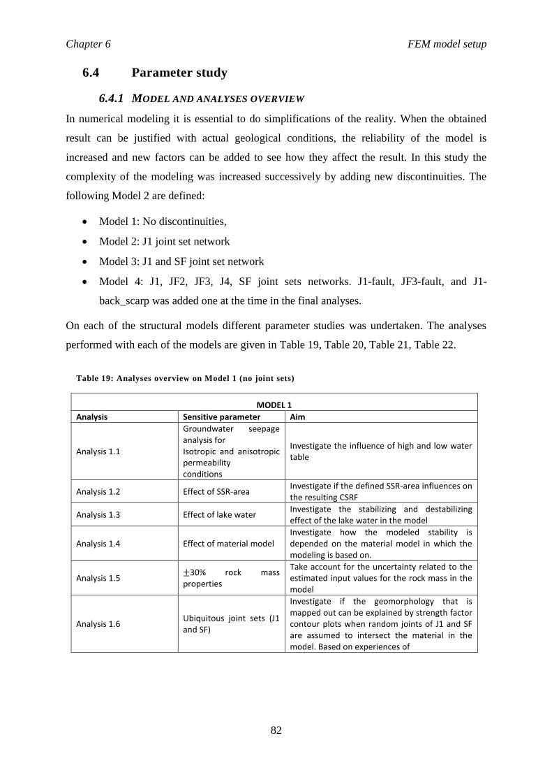
Chapter 6 FEM model setup
82
6.4 Parameter study
6.4.1 MODEL AND ANALYSES OVERVIEW
In numerical modeling it is essential to do simplifications of the reality. When the obtained
result can be justified with actual geological conditions, the reliability of the model is
increased and new factors can be added to see how they affect the result. In this study the
complexity of the modeling was increased successively by adding new discontinuities. The
following Model 2 are defined:
Model 1: No discontinuities,
Model 2: J1 joint set network
Model 3: J1 and SF joint set network
Model 4: J1, JF2, JF3, J4, SF joint sets networks. J1-fault, JF3-fault, and J1-
back_scarp was added one at the time in the final analyses.
On each of the structural models different parameter studies was undertaken. The analyses
performed with each of the models are given in Table 19, Table 20, Table 21, Table 22.
Table 19: Analyses overview on Model 1 (no joint sets)
MODEL 1
Analysis Sensitive parameter Aim
Analysis 1.1
Groundwater seepage analysis for Isotropic and anisotropic permeability conditions
Investigate the influence of high and low water table
Analysis 1.2 Effect of SSR-area Investigate if the defined SSR-area influences on the resulting CSRF
Analysis 1.3 Effect of lake water Investigate the stabilizing and destabilizing effect of the lake water in the model
Analysis 1.4 Effect of material model Investigate how the modeled stability is depended on the material model in which the modeling is based on.
Analysis 1.5 ±30% rock mass properties
Take account for the uncertainty related to the estimated input values for the rock mass in the model
Analysis 1.6 Ubiquitous joint sets (J1 and SF)
Investigate if the geomorphology that is mapped out can be explained by strength factor contour plots when random joints of J1 and SF are assumed to intersect the material in the model. Based on experiences of

Chapter 6 FEM model setup
83
Table 20: Analyses overview in Model 2 (J1 joint set)
MODEL 2
Analysis 2.1 Model with J1 joint network. Two structural domains. Initial values.
Investigate how the stability in the rock mass changes when discontinuous joints dissect the material.
Analysis 2.2-2.5 Parameter study of friction angle in the rock mass
Investigate how the stability in the rock mass changes with decreased shear strength
Analysis 2.6-2.9 Parameter study of cohesion in the rock mass
Investigate how the stability in the rock mass changes with decreased shear strength
Analysis 2.10 1) 12% reduced φ 2) 48% reduced c.
Comparing two conditions of equal stability but different rock mass parameter values
Analysis 2.11 1) 50% reduced φ 2) 50% reduced c
Investigate contour plots for a unstable slope condition
Analysis 2.12 30% reduced φ and 50% reduced c a) high water table b)low water table
Investigate contour plots for a that is assumed to be the best reflection of the actual conditions in the slope
Analysis 2.13 Parameter study joint property, JRC, JCS and
Investigate the sensitivity of slope stability due to joint strength parameters of J1
Table 21: Analyses overview of Model 3 (J1 and SF)
MODEL 3
Analysis 3.1 Model with J1 and SF discontinuities
Investigate the sensitivity of slope stability due to joint network properties of SF
Analysis 3.2-3.3 Parameter study on joint network property: persistence
Analysis 3.4-3.7 Parameter study of joint property: stiffness
Analysis 3.8-3.9 Parameter study of joint network property: length and persistence
Table 22: Analyses overview Model 4 (all discontinuities)
MODEL 4
Analysis 4.1 All joint sets added Investigate the slope condition changes when all joint sets are added in the model
Analysis 4.2 J1-fault, JF3-fault, back scarp, all joints
Investigate the effect of adding major geological structures mapped in field

Chapter 7 Results structural analysis
84
7 RESULTS
7.1 Results from structural analysis of TLS-data in Coltop
In order to reduce the uncertainty of the structural model obtained in the project assignment, a
supplementary analysis of terrestrial lidar scan data (TLS) was performed in the 3D Lidar data
analyzing software COLTOP. The aim with this supplementary structural analysis is to
support the field orientation measurements and the reliability of the subdivision of joint sets
defined in the project assignment, and to control if there are structures on the slope that were
missed during field mapping.
7.1.1 RESULTS FROM DISCONTINUITY MAPPING IN COLTOP
Figure 28 show the point cloud model of the Håkåneset rock slide that was used for the
structural analysis in COLTOP. The model is based on terrestrial laser scans from two
directions, obtained by NGU in 2012. The software PolyWorks was used to clean, combine
and georeference the scans before the model was exported to COLTOP.
Figure 28: Print screen from the structural analyzing software COLTOP, showing the colored point
cloud model of the study area at Håkåneset. The model is obtained by terrestrial laser scan from two
directions in 2012.

Chapter 7 Results structural analysis
85
The COLTOP-model reflects exposed surfaces as areas with homogeneous color in the point
cloud, as described in Chapter 4.2.1 and Figure 12. The surfaces are interpreted to reflect the
discontinuity sets that are present in the rock masses on the slope. In the Håkåneset model, six
different colors were mapped out: green, yellow, turquoise, pink, purple and light
yellow/green, see Figure 29.
10-30 surfaces of each color-selection were mapped out by drawing polygons. The output of
these polygons is a high number of orientation (Dip direction/Dip) measurements. The
number of measurements is referred to as #Points in Table 23. Some brief observations for
each color-selection is listed in Table 23. Several of the selections are pronounced only as
small surfaces that were difficult to define without including many scatter points, resulting in
a relative wide standard deviation. Also, since the joint sets in Håkåneset in general are
vertically dipping, points in one surface might have a 180 degree difference in dip direction,
and consequently the color of the surface will not be homogeneous (Selection 4: yellow/blue
is a good example).
Figure 29: COLTOP displays exposed surfaces as areas with homogeneous color. The surfaces are
interpreted to reflect the discontinuities that are present in the rock mass. Six color selections were
defined and mapped out in the Håkåneset: turquoise, green, yellow/blue, light yellow/green, pink and
purple.

Chapter 7 Results structural analysis
86
The orientation of the six color-selections was determined by exporting the selected
orientation data into the structural orientation analyzing software DiPS 6.0 (Rocscience). First
the analysis was performed with data from the whole area. Second, data for each structural
domain (North, Lower-South and Upper-South) were exported to DiPS separately and
analyzed. The subdomains were defined in the project assignment, due to a systematic spatial
structural variability in the slope, see Figure 19. Joint set orientations were determined by
cluster analysis in contour plots (lower hemisphere, equal area, Fisher distribution). The
Table 23: Surface selections mapped in the COLTOP-model. All data plotted in a stereographic
projection pole plot.
Color Selection #Surfaces #Points Observation Sterographic projection
turquois 1 24 10336 Mainly in the upper south domain.
Dominant systematic joints in the block area in the upper south domain.
green 2 30 22658 Big slope parallel surfaces in the back wall.
The most pronounced color in the entire slope.
pink 3 30 4581 Only small surfaces.
Visible in the whole model.
Variable density.
yellow/blue 4 19 7739 Best pronounced in the road cut.
Often together with green color.
purple 5 11 3149 Only pronounced in the Lower-South domain: in the block area and in the road cut directly under the block area.
Only small surfaces.
Often together with pink.
light yellow/green
6 20 25249 Big slope parallel surfaces.
Dominant color in the lower part of the slope.
Not seen in the back wall.

Chapter 7 Results structural analysis
87
contour range was set to 2 -10 and 10 intervals, and the joint sets were defined by drawing a
window covering all measurements within this contour range. Due to this setting some joint
sets are not statistically significant, thus orientation data are not determined for these joint sets
in the particular domains. The result is given in Table 24 as mean orientations (Dip
direction/Dip) and its standard deviation. The same procedure has been performed on the
orientations measurement data from the field mapping, given in Table 5.
Table 24: Results of structural analysis of TLS-data in Coltop, given as mean orientation (Dip
direction/Dip) and standard deviation of identified surface color selections.
Domains
Colour Entire study area North Lower-South Upper-South Back Wall
Sele
ctio
n
1 turqouis 15°/60° ± 19° 26°/47° ± 19° 11°/67° ± 18° 10°/56° ± 10° 17°/67° ± 15°
2 green 66°/67° ± 16° 67°/65° ± 17° 71°/67° ± 17° 68°/65° ± 17° 63°/68° ± 13°
3 pink 221°/79° ± 18° 232°/76° ± 15° 216°/79° ± 15° 211°/81° ± 15° 234°/79° ± 15°
4 yellow/blue 122°/75° ± 19° 125°/69° ± 17° 123°/76° ± 17° - 108°/76° ± 19°
5 purple 260°/73° ± 18° - 258°/74° ± 17° - -
6 yellow/white 80°/44° ± 21° 77°/54° ± 23° 80°/43° ± 21° 89°/41° ± 19° -

Chapter 7 Results structural analysis
88
Ta
ble
25
: Disc
on
tinu
ity o
rie
nta
tion
s (Dip
dir
ectio
n/D
ip) o
bta
in b
y str
uctu
ra
l an
aly
sis of fie
ld m
ea
sur
em
en
ts field
mea
sur
em
en
ts co
mp
are
d to
disc
on
tinu
ity o
rie
nta
tion
s ob
tain
ed
b y
stru
ctu
ra
l an
aly
sis of T
LS
- da
ta in
CO
LT
OP
- 3D
7.1.2 COMPARING STRUCTURAL ORIENTATION MEASUREMENTS: TLS VS.
FIELD
The discontinuity orientations mapped in TLS-model,
Table 24, was compared to the discontinuity
orientations mapped in field, Table 5. It is clear that all
selections from COLTOP can be related to one of the
joint sets defined from the field measurements:
Selection 1, turqouis surfaces, corresponds to the
tectonic joint set JF2.
Selection 2, green surfaces, corresponds to the
slope parallel exfoliation joint set J1 in the
steepest parts of the slope.
Selection 3, pink surfaces, corresponds to joint
set J4.
Selection 4, yellow/blue surfaces, corresponds to
the tectonic joins set JF3.
Selection 5, purple surfaces, can be J1 or J4, see
discussion in point 3) below.
Selection 6, light yellow/green surfaces,
corresponds to the slope parallel exfoliation joint
set J1 in the shallowest part of the slope.
The structural analysis of TLS-data confirms that all
dominant joint sets in the Håkåneset rock slope were
mapped. Table 25 present the comparison between
discontinuity orientations (Dip direction/Dip) derived
from field data and from TLS-data. Data for each
defined joint set is given for the entire study area and for

Chapter 7 Results structural analysis
89
each subdomain. Some important trends are observed when comparing the data sets:
1. Selection 2 (green) and Selection 6 (light yellow/green) can be distinguished as
separate selections, but both are observed as slope parallel surfaces in the TLS-model,
thus interpreted as an exfoliation joint. The orientations of Selection 2 and Selection 6
are labeled as J1-1 and J1-2, respectively in Table 25. For all domains the orientation
of the field mapped data is approximately the average value of the TLS-data based
joint sets J1-1 and J1-2.
2. J1-1 is oriented NE and dips with a steeper angle than J1-2. J1-2 is oriented more
towards east than J1-1 in all domains. In addition, J1-1 is observed as most dominant
in the Upper-South domain and J1-2 is observed as most dominant in the Lower-South
domain. The latter can be seen visually in Figure 31, as the point cloud appear green
and yellow in the upper parts, and more light yellow towards the lower part. Thus, it is
reasonable to assume that the dip angle of the exfoliation joint in general is stepper in
the upper part than in the lower part of the slope. The same trend that was observed in
the structural analysis of the field measurements in the project assignment, and was
the reason for the subdivision between the two southern structural domains (Lower-
South and Upper-South). The results from the COLTOP analysis support this
subdivision.
3. J1_3 is represented by the surfaces mapped out as Selection 5. This joint set could
either be included in Selection 3, indicate that joint set J4 has a wide range of dip
direction, or they can be included in Selection 2 as a variance of the steeply dipping
exfoliation joint set J1. The latter has been assumed as most likely due to the
following reason: The morphology on the slope in the study area is assumed to be
defined by slow deformation along reactivated inherited structures. However, the
dominant exfoliation joint set is by definition not a reactivated joint set, but rather a
result of this reactivation due to stress relief during the deformation. Consequently, it
is reasonable to include J1_3 surfaces in the exfoliation joint set, even though it is not
surface parallel, because J1_3 can be assumed to reflect a steeply dipping inherited
structure that defined the formation of exfoliation. Because the morphology on the
slope of the study area reflects the dominance of the J1 structure, while J4 is not
observed as a regional structure in the study area, the explanation of Selection 5 being
a variance of J1 rather than a variance of J4 is assumed as most likely.

Chapter 7 Results structural analysis
90
4. For JF2 and JF3 there is a consistent 10-20 degree bias between the dip directions of
the field mapped data and TLS mapped data. For JF2 this bias is clockwise towards
and for JF3 this bias is counterclockwise. An possible explanation of this bias is:
5. Foliation planes are not mapable in the TLS data model in COLTOP. This is as
expected since the foliation seen in field was dipping with a low angle, and will
therefore be approximately parallel with the laser beam. Consequently, foliation
planes are not covered in the point cloud model. This highlights the importance of
field mapping in order to detect all discontinuities that are present in a rock mass.
7.1.3 CONCLUSION
The structural analysis of LiDAR-data in Coltop support the reliability the field
measurements, and indicate that all discontinuity sets that are dominant in the slope have been
mapped in the field. There is no significant difference in the estimated orientation data
derived with the two applied approaches. Therefore, the kinematic model obtained in the
project assignment can be considered as representative for the Håkåneset rockslide, and is
considered a good basis for further stability analysis of the rockslide.
Figure 30: In Polyworks the colored surfaces are
obtained by interpolation of a plane between two
scan directions. This might cause a bias due to the
scan direction This is likely to be the reason for the
systematic difference between the field orientation
measurements and the TLS orientations
measurements of JF2 and JF3.

Chapter 7 Results structural analysis
91
Figure 31: A systematic structural variability in the exfoliation joint set J1 is observed: the upper
and central part is colored green and yellow, respectively, and the lower part is colored more
light yellow. From the stereographic plots in the left corner this color trend indicate that the
upper part of the slope is dominated by more steeply dipping surfaces than the lower part. The
same trend was observed in the field mapped data in the project assignment.

Chapter 7 Deformation analysis in Polyworks
92
7.2 Results from deformation analysis of TLS-data in Polyworks
A deformation analysis of the instability at Håkåneset was performed in order to identify
displacements of rock masses and the volume of these. TLS-data models from 2012 and 2013
were compared to search for significant displacement.
No critical areas with significant displacement can be reported for the study area after the
performed stability analysis in IMInspect, Polyworks. However, it is important to highlight
that the data TLS-data models used for the analysis were limited. These limitations are due to
vegetation cover, resulting in a model with decreasing points density for the southern part of
the slope. Because of this the combination and comparison of the models was difficult, which
lower the reliability of the results.
Figure 32 is the output model from the comparison of the 2013 model with respect to the
2012 model in IMInspect. The color codes are used to interpret the displacement activity in
the slope. Note that grey color represents areas that have not been cleaned for vegetation in
the 2013 TLS-data. The following conclusions can be interpreted from the performed
analysis:
1. As a first step in the analysis the models from 2012 and 2013 was combined taking
only the assumed stable areas, i.e. the northern part (right) and the upper most part of
the slope into account. This procedure is undertaken by ignoring the points of the
assumed unstable areas. Green color represents areas that have been nicely fitted, and
by this it is seen that the fit alignment is good in the right part of the model. A green
color would also be expected in the uppermost part of the slope, since this is defined
as the back scarp of the instability. However, the error seems to increase towards the
left of the model - indicated with more yellow and red colors. This is a clear indication
of the limitations of the model that has been used for this displacement analysis, as
regards insufficient point density of the left part of the model. This observation has to
be remembered for further interpretation of the color codes within the limits of the
unstable rock masses.
2. Blue color is pronounced in the parts representing the upper block area. The blue color
indicates a negative rock mass volume, and could therefore be interpreted a sign of
significant rock fall. However, when further investigating theses blue areas, it was
revealed the 2012 scan has a limit in this part, see Figure 33. Consequently, large
errors occur when the 2013 scan is compared to the reference scan in this region
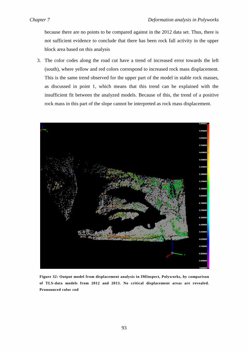
Chapter 7 Deformation analysis in Polyworks
93
because there are no points to be compared against in the 2012 data set. Thus, there is
not sufficient evidence to conclude that there has been rock fall activity in the upper
block area based on this analysis
3. The color codes along the road cut have a trend of increased error towards the left
(south), where yellow and red colors correspond to increased rock mass displacement.
This is the same trend observed for the upper part of the model in stable rock masses,
as discussed in point 1, which means that this trend can be explained with the
insufficient fit between the analyzed models. Because of this, the trend of a positive
rock mass in this part of the slope cannot be interpreted as rock mass displacement.
Figure 32: Output model from displacement analysis in IMInspect, Polyworks, by comparison
of TLS-data models from 2012 and 2013. No critical displacement areas are revealed.
Pronounced color cod

Chapter 7 Deformation analysis in Polyworks
94
Conclusion of displacement analysis
Due to the quality of the data set the analysis is dominated by a systematic error because the
fit alignment between the temporal models is bad. Thus, the results obtained by the analysis in
this study cannot be used for further discussion of the slope stability condition at Håkåneset.
Figure 33: In the left figure both 2012 and 2013 data are displayed. In the right figure only 2013 data
are visible. It is clear that the 2012 scan has a limit in the area, indicated with the red dotted line, that
results in blue color (negative volumes). Thus, there is not sufficient evidence to conclude that there has
been rock fall activity in the upper block area based on this analysis.

Chapter 7 Results numerical modeling
95
7.3 Results of stability analysis with numerical modeling in
Phase2
This chapter presents the results obtained by numerical modeling using a finite element
method (FEM) with a shear strength reduction (SSR) approach. Four structural models have
been investigated by successively adding new discontinuities. The stability has been
investigated by parameter sensitivity tests for different hydrogeological conditions and rock
mass and joints properties, resulting in different critical strength reduction factor (CSRF). As
a vital achievement of the stability analysis of the Håkåneset rockslide is to predict the most
likely location and geometry of a potential sliding surface in case of a large-scale slope
failure. This is done by visual analysis where maximum shear strain plots are used to interpret
active-passive zones. According to Stead and Eberhardt (2013) will the failure surface
geometry have a significant influence on the rock slope damage. With this, evaluation of
shear strain at different slope conditions is justified as an efficient approach for indicating a
probable sliding plane. Contour plots for total displacement, horizontal displacement and
vertical displacement have also been interpreted in the study. When reading the results it is
important to remember that the contour range values differs for each plot, and consequently
the colors can only be used for interpreting relative changes within one plot and not for
comparison of different analyses
An overview of performed analyses was given in Table 19, Table 20, Table 21 and Table 22.
When a model for numerical modeling is constructed, it is necessary to do significant
simplifications of the reality. It must be emphasized that the result from a numerical modeling
can never be of better reliability than the quality of the input data. Several uncertainties are
discussed for the input values used in this study, related both to the model itself and to the
rock mass input parameters. This must always be kept in mind when interpreting the results,
and they should never be trusted as finite answers.
7.3.1 GROUNDWATER SEEPAGE ANALYSIS
This study uses a groundwater seepage analysis to model a groundwater table based on
assumed hydraulic rock mass properties. Since there exist no hydraulic data and the
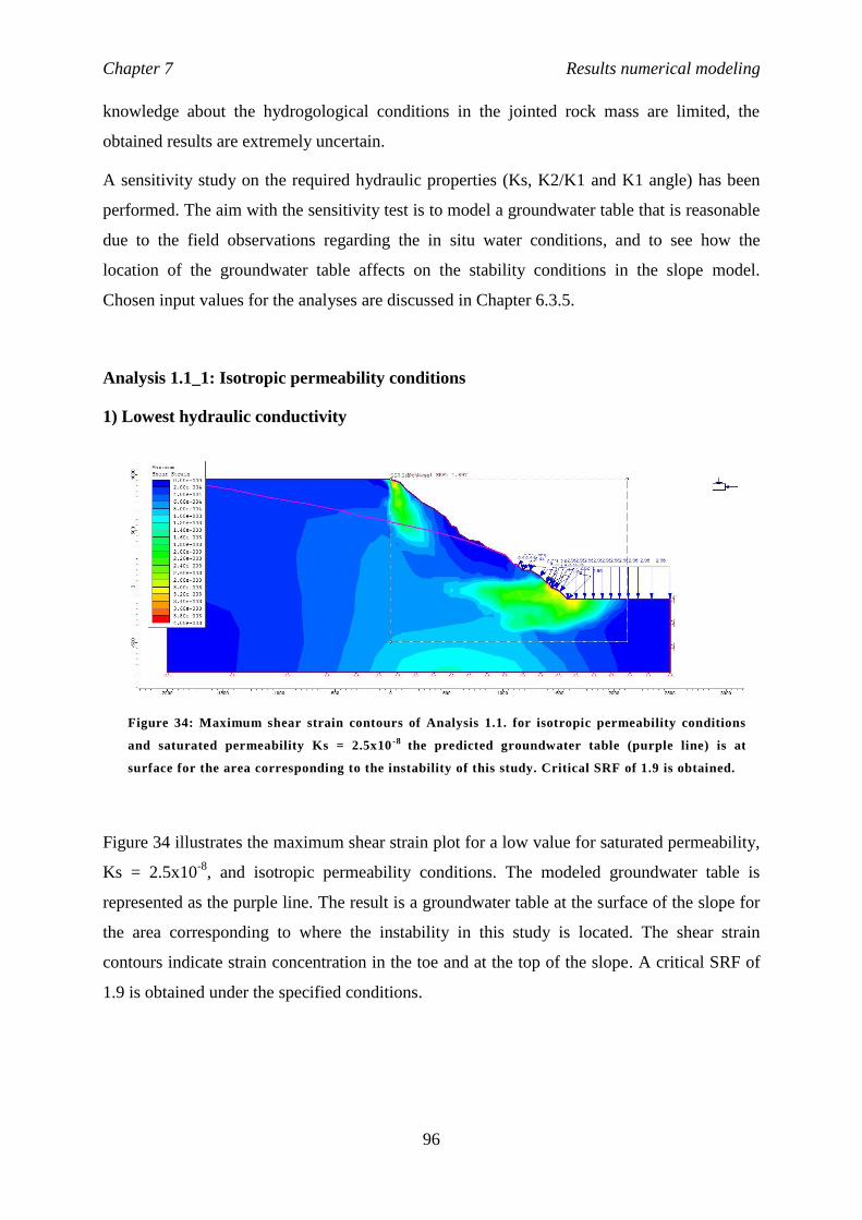
Chapter 7 Results numerical modeling
96
knowledge about the hydrogological conditions in the jointed rock mass are limited, the
obtained results are extremely uncertain.
A sensitivity study on the required hydraulic properties (Ks, K2/K1 and K1 angle) has been
performed. The aim with the sensitivity test is to model a groundwater table that is reasonable
due to the field observations regarding the in situ water conditions, and to see how the
location of the groundwater table affects on the stability conditions in the slope model.
Chosen input values for the analyses are discussed in Chapter 6.3.5.
Analysis 1.1_1: Isotropic permeability conditions
1) Lowest hydraulic conductivity
Figure 34 illustrates the maximum shear strain plot for a low value for saturated permeability,
Ks = 2.5x10⁻⁸
, and isotropic permeability conditions. The modeled groundwater table is
represented as the purple line. The result is a groundwater table at the surface of the slope for
the area corresponding to where the instability in this study is located. The shear strain
contours indicate strain concentration in the toe and at the top of the slope. A critical SRF of
1.9 is obtained under the specified conditions.
Figure 34: Maximum shear strain contours of Analysis 1.1. for isotropic permeability conditions
and saturated permeability Ks = 2.5x10 -8 the predicted groundwater table (purple line) is at
surface for the area corresponding to the instability of this study. Critical SRF of 1.9 is obtained.

Chapter 7 Results numerical modeling
97
Justifying the SSR-area
The dotted square in Figure 34 represents the defined SSR-area that is defined in order
to get the most time effective model. Before the analysis of geological factors could
start, it was considered necessary to investigate if the SSR-area influenced the result.
When Analysis 1.1 was run without a SSR-area (referred to as Analysis 1.2 in Table
19) the CSRF and strain concentration zones were not significantly changed. Hence,
the application of SSR-area in the model could be considered justified as not affecting
the results of further modeling.
Analysis1.1_2: Highest hydraulic conductivity
Figure 35 illustrate the resulting shear strain conditions for Analysis 1.1_2 that assumes
isotropic hydraulic conductivity that is a factor of 106 higher than assumed in Analysis 1.1_1.
The groundwater table follows the slope surface in the area corresponding to the location of
the Håkåneset instability, and the CSRF is unchanged 1.9 to the value obtained in Analysis
1.1_1. Strain concentration is predicted in the toe and at the top of the mountain slope. Thus,
the result of Analysis 1.1_1 and Analysis 1.1_2 indicate that the magnitude of the hydraulic
conductivity over the range that is assumed reasonable for the jointed rock mass at Håkåneset
does not have a significant effect on the slope stability. Due to this observation it was decided
to base further modelling on the mean hydraulic conductivity of 5.0 10-5
.
Figure 35: Maximum shear strain contours of Analysis 1.1 for isotropic permeabilit y conditions and
saturated permeability Ks=1x10 -2. The predicted groundwater table (purple line) and CSRF are
unchanged compared to Analysis 1.1_1.

Chapter 7 Results numerical modeling
98
Analysis 1.1_3: Anisotropic permeability conditions
Figure 36 is the resulting shear strain plot when an anisotropic permeability condition is
defined, assuming vertical groundwater flow with the horizontal permeability being a factor
of 0.001 of vertical (Ks = 5.0 10-5
). Under these settings a subsurface groundwater table
(purple line) is predicted. Critical SRF is obtained for the value of 2.1. Strain concentrations
are predicted in the same regions and of the same magnitude as in Analysis1.1_1-2 where the
groundwater table was at surface.
Figure 36: A subsurface groundwater table is predicted when an anisotropic permeability conditions
with dominant vertical water flow is assumed. Vertical permeability defined as equal to Ks= 5,0 10-5
and horizontal permeability a factor of 0.001 to the vertical. CSRF of 2,1 is obtained.

Chapter 7 Results numerical modeling
99
7.3.2 EFFECT OF SUBMERGED-SUBAQUATIC INSTABILITY
Analysis 1.3 is conducted with the same settings as the anisotropic hydraulic model in
Analysis 1.1_3, but with no lake water (pounded water and water load excluded). A critical
SRF value of 2,1 is obtained. From Figure 37 show that strain concentrations are predicted at
the top of the mountain slope and horizontally from the toe and into the slope.
Figure 37: Maximum shear strain plot for a model without the lake water. Same model setting as in
Analysis 1.1 with anisotropic conditions. CSRF value of 2.1 is obtained.

Chapter 7 Results numerical modeling
100
7.3.3 SHEAR STRENGTH REDUCTION (SSR) ANALYSIS
Model 1 is a topographic model with no discontinuities. A plot summarizing the resulting
CSRF for each analysis with Model 1 is given in Figure 38, and more detailed description is
given in the following text. Also the results from the analyses regarding the hydrogeological
conditions (Chapter 7.3.1-2) are plotted. The trend in Figure 38 indicates that the slope
stability is most sensitive to factors that material properties are dependent on (material model,
material strength).
Figure 38: Summary of tested parameters with Model 1.
0
0,5
1
1,5
2
2,5
3
3,5
4
0 20 40 60 80
Cri
tica
l str
en
gth
re
du
ctio
n f
acto
r (C
SRF)
Peak friction angle
Sensitivity study Model 1 (no joint sets)
Initial rock mass properties and surface parallel GW 30% reduced rock mass properties
30% increased rock mass properties
Subsurface water table
Ubiquitous joints (J1, SF)
No SSR area
Elastic-perfectly plastic material model (Analysis 1.4) No lake water, subsurface groundwater table

Chapter 7 Results numerical modeling
101
Influence of material model (Analysis 1.4)
Analysis 1.1-3 assumes elastic-plastic softening material model. The choice of a material
model is essential for the modeling result and therefore important to investigate.
In Analysis 1.4 an elastic-perfectly plastic (EPP) materiel model was assumed, that imply
residual strength parameters equal the peak friction angle. Isotropic permeability was assumed
to get the most conservative analysis. Compared to the model with elastic-plastic softening
and isotropic hydraulic properties in Analysis 1.1, the CSRF was increased from 1.9 to 3.8 for
the EPP model. The shear strain plot for the EPP model setup in Figure 39A indicates a
continuous circular maximum strain concentration starting from the mountain plateau and
daylighting at the level of the lake surface. In addition, maximum strain is expected in a small
area at approximately 100 m depth. The total displacement plot in Figure 39B indicates a
decreasing displacement from surface and into the slope, with maximum displacement at the
top of the mountain slope, i.e. outside the area corresponding to the location of the Håkåneset
rockslide. In Analysis 1.1 on the other hand, where residual strength was assumed to be 2/3 of
the peak value, most significant displacement was indicated in an area of the model that
correspond to the submerged domain of the defined instability. The slope conditions indicated
in Analysis 1.1 is to reflect the actual conditions in the slope in a better way than Analysis
1.4. Based on this it was decided to continue the further stability analysis in Phase2 with an
elastic-plastic softening material model, with residual material strength values assumed as 2/3
of the peak values.
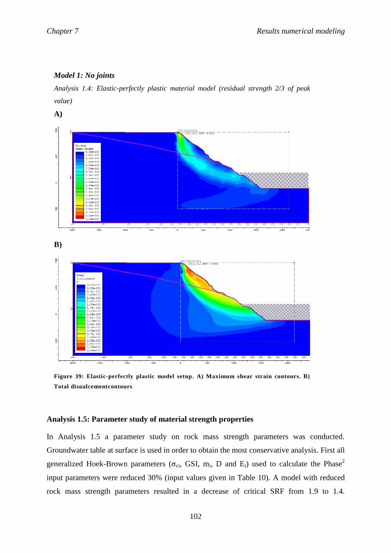
Chapter 7 Results numerical modeling
102
Analysis 1.5: Parameter study of material strength properties
In Analysis 1.5 a parameter study on rock mass strength parameters was conducted.
Groundwater table at surface is used in order to obtain the most conservative analysis. First all
generalized Hoek-Brown parameters (σci, GSI, mi, D and Ei) used to calculate the Phase2
input parameters were reduced 30% (input values given in Table 10). A model with reduced
rock mass strength parameters resulted in a decrease of critical SRF from 1.9 to 1.4.
Model 1: No joints
Analysis 1.4: Elastic-perfectly plastic material model (residual strength 2/3 of peak
value)
A)
B)
Figure 39: Elastic-perfectly plastic model setup. A) Maximum shear strain contours. B)
Total dispalcementcontours

Chapter 7 Results numerical modeling
103
Maximum shear strain contours for this model setup is shown in Figure 40A), where strain
concentration is indicated in the lower part of the slope, thus it coincides with the location of
the unstable area. Figure 40B) show that maximum total displacement is indicted in the
submerged component of the unstable slope.
Secondly, the generalized Hoek-Brown parameters were increased with 30% (Table 10),
resulting in increasing critical SRF from 1.9 to 2.6. Figure 41A shows that a model setup with
Model 1: No joints
Analysis 1.5: 30% reduced rock mass strength
A)
B)
Figure 40: A) Maximum shear strain contour plot and B) Total displacement contour plot for 30%
reduced rock material properties (Analysis 1.4).

Chapter 7 Results numerical modeling
104
increased material strength properties predict a circular shaped maximum shear strain
concentration area starting at the top of the mountain slope and continue down to the toe.
Again the total displacement plot in Figure 41B indicates most displacement activity in the
central part of the submerged slope component.
Model 1 with ubiquitous joints J1 and SF (Analysis 1.6)
In Analysis 1.6 J1 and SF joint sets were added to the Model 1 as ubiquitous joints.
Groundwater table at surface is used in order to obtain the most conservative analysis. From
Model 1: No joints
Analysis 1.5: 30% increased rock mass strength
A)
B)
Figure 41: A) Maximum shear strain contour plot and b) Total displacement contour plot for 30%
increased rock material properties (Analysis 1.5).

Chapter 7 Results numerical modeling
105
the kinematic feasibility test (see Chapter 5.4.2) it was concluded that the exfoliation joint set,
J1, and the schistose foliation joint set, SF, are the most interesting joint sets for further
investigation of the slope stability at Håkåneset regarding a massive slope failure. Therefore,
these joint sets were included as ubiquitous joint sets in the stress calculations of Model 1, in
order to get a first impression whether the stresses generated from the finite element analysis
are sufficient to cause slip along planes with J1 and SF orientation based on the specified
discontinuity strength parameters only. Barton-Bandis joint strength input parameters values
is given in Table 14.
The resulting strength factor contour plot of Model 1 is presented in Figure 42. By definition,
the factor of safety (strength factor) is the shear strength divided by the shear stress, implying
that a FoS less than 1 indicate slip. In Figure 42A) only J1 is added as a ubiquitous joint in the
model. The field estimate of JRC = 14 for J1 joint surfaces gave no critical FoS in the slope
model. However, by reducing JRC to 5, the contour plot in Figure 42A) was obtained,
indicating two critical areas in the submerged part of the slope. In Figure 42B) SF is added in
addition to J1, resulting in expected FoS less than 1 in the region of Model 1 that corresponds
to the limits of the instability of this study.
The result from the ubiquitous joint option supports the assumption of J1 and SF as critical
structural factors regarding the slope stability at Håkåneset, thus the importance of J1 and SF
properties was prioritized for the continuing numerical modeling .

Chapter 7 Results numerical modeling
106
Model 1: No joins
A) Analysis 1.6a: Ubiquitous joints J1
B) Analysis 1.6b: Ubiquitous joints J1 and SF
Figure 42: Strength Factor contour plots when A) J1 and B) J1and SF are added as
ubiquitous joints in Model 1. The area indicating critical conditions regarding failure
(orange contour) increases from plot A) to B).
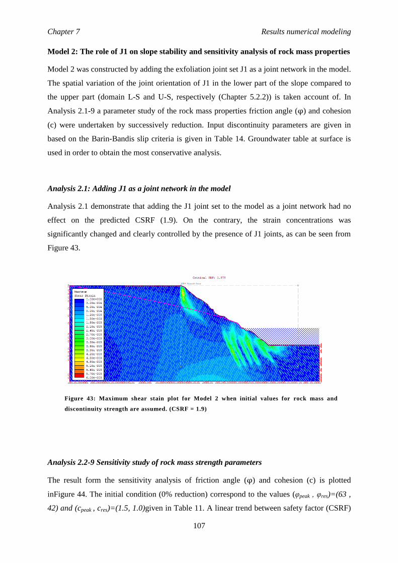
Chapter 7 Results numerical modeling
107
Model 2: The role of J1 on slope stability and sensitivity analysis of rock mass properties
Model 2 was constructed by adding the exfoliation joint set J1 as a joint network in the model.
The spatial variation of the joint orientation of J1 in the lower part of the slope compared to
the upper part (domain L-S and U-S, respectively (Chapter 5.2.2)) is taken account of. In
Analysis 2.1-9 a parameter study of the rock mass properties friction angle (φ) and cohesion
(c) were undertaken by successively reduction. Input discontinuity parameters are given in
based on the Barin-Bandis slip criteria is given in Table 14. Groundwater table at surface is
used in order to obtain the most conservative analysis.
Analysis 2.1: Adding J1 as a joint network in the model
Analysis 2.1 demonstrate that adding the J1 joint set to the model as a joint network had no
effect on the predicted CSRF (1.9). On the contrary, the strain concentrations was
significantly changed and clearly controlled by the presence of J1 joints, as can be seen from
Figure 43.
Analysis 2.2-9 Sensitivity study of rock mass strength parameters
The result form the sensitivity analysis of friction angle (φ) and cohesion (c) is plotted
inFigure 44. The initial condition (0% reduction) correspond to the values (φpeak , φres)=(63 ,
42) and (cpeak , cres)=(1.5, 1.0)given in Table 11. A linear trend between safety factor (CSRF)
Figure 43: Maximum shear stain plot for Model 2 when initial values for rock mass and
discontinuity strength are assumed. (CSRF = 1.9)

Chapter 7 Results numerical modeling
108
and parameter reduction is observed for both φ and c where CSRF is more sensitive to
variations of φ than variations of c.
In Figure 45 rock mass parameter reduction is plotted in relation to the shear strength for a
normal stress level of 1,4MP. (Shear strength is calculated with Eq. 2).
Figure 44: Result of parameter study of Model 2 by reducing friction angle and cohesion
separately. CSRF appears as most sensitive to reduction in friction angle.
0
0,2
0,4
0,6
0,8
1
1,2
1,4
1,6
1,8
2
0 % 20 % 40 % 60 % 80 % 100 %
Cri
tica
l SR
F
Parameter reduction
Sensitivity study of rock mass shear strenght parameters on Model 2 (Joint set J1)
Friction angle
Cohesion
Figure 45: Shear strength sensitivity due to reduction of friction
angle (red) and cohesion (blue). Calculations assumed that normal
stress level is 1,4MPa.
0
0,5
1
1,5
2
2,5
3
3,5
4
4,5
0 % 10 % 20 % 30 % 40 % 50 % 60 % 70 % 80 % 90 %
She
ar s
tre
ngt
h,
Rock mass parameter reduction

Chapter 7 Results numerical modeling
109
From the relations in Figure 45 it can be read that a 12% reduction of friction angle should
result in the same shear strength as 48% reduction of friction angle. Since CSRF by definition
depends on the shear strength, it is expected that the two different models should indice the
same CSRF. This is confirmed in Analysis 2.10. On the contrary, the strain concentrations
plots are significantly different in the case with 12% reduced cohesion compared to when
only the friction angle is reduced 48%, as illustrated in Figure 46.
Analysis 2.11 demonstrates the expected slope conditions when a unstable condition with a
safety factor less than 1 is indicated. According to the trend in Figure 44 a critical slope
A) 12% reduced phi
B) 48% reduced cohesion
Figure 46: A) 48% reduced cohesion correspond to B) 12% reduced friction angle to obtain the
same shear strength level and equal CSRF for both conditions. Even though the CSRF is equal,
the strain concentration for the two conditions are significantly different.

Chapter 7 Results numerical modeling
110
condition with Safety Factor equal 1,0 should be obtained if the friction angle is reduced by
50% due to the initial values, Table 11. Figure 47A) shows maximum shear strain plot when
the friction angle is reduced with 50% and a critical condition with CSRF less than 1 is
obtained. Most significant shear strain is expected from the central part of the submerged
slope component and dipping into the slope. In Figure 47B it can be seen that most significant
total displacement is indicated from the level of the central part of the submerged slope.
To compare, a model set up with 50% reduced cohesion was conducted, resulting in the
contour plots seen in Figure 48. The shear strain plot in Figure 48A indicate maximum strain
concentration in four zones that are dipping parallel with the J1 joints. Most significant
Model 2: Joint set J1
Analysis 2.11_1): 50% reduced friction angle
A)
B)
Figure 47: Model 2 with 50% reduced friction angle gives a safety factor of 1.0, which indi cate
unstable slope conditions. A) Maximum shear strain contour plot and B) Total displacement
contour plot.

Chapter 7 Results numerical modeling
111
displacement, Figure 48B, is indicated in the part of the slope that is at the level of the lake
level.
Based on the results presented above, it was concluded that conditions that bring the slope
towards a critical state of failure can be obtained by reduction of friction angle, while
reduction of the cohesion gives a strain condition that best describes the mapped morphology
in the slope. By combining these experiences, Analysis 2.12a was conducted with a material
Model 2: Joint set J1
Analysis 2.11_2): 50% reduced cohesion
A)
B)
Figure 48: Model 2 with 50% reduced cohesion gives a safety factor of 1.7, which indicate stable slope
conditions. A) Maximum shear strain contour plot and B) Total displacement contour plot . In this case
the most active zone is indicated closer to lake surface level.

Chapter 7 Results numerical modeling
112
model with 30% reduced friction angle and 50% reduced cohesion to initial values.
Groundwater conditions were set as conservative with groundwater table at surface. This
material model setup was found by trial as the condition that brings the SRF close to the
critical state at 1 and at the same time is closest to reflect the observed geomorphology in the
slope. However, it is important to remember that this visual analysis is also fully dependent
on other input parameters (tensile strength, E-modul, joint surface strength, hudraulic
properties etc.) that are not tested for, thus the obtained values for φ and c that leads to a
model condition that indicate failure cannot be taken as true critical values. The result of the
model setup in Analysis 2.12 is illustrated in Figure 49. For this model set up a CSRF 1.06
was obtained when a high water table is assumed for a conservative analysis. Maximum shear
strain zones in Figure 49A) are parallel to J1 orientation in the lower part of the model. In
addition, strain condition is indicated at the top of the entire mountain slope. Figure 49B)
indicate that most significant total displacement should be expected in a subsurface area
(red/yellow contours) at a lake bottom level, while the horizontal displacement (abs) plot in
Figure 49C) indicate most significant displacement (relative to CSRF=1) in the submerged
component of the instability from the central area and up to the lake surface level.
Analysis 2.12b assumed anisotropic permeability and a subsurface ground water table a CSRF
of 1.1 was obtained. The contour ranges for the anisotropic hydraulic condition is presented in
Appendix 8.1, showing that the contour are only slightly different to the isotropic hydraulic
condition.

Chapter 7 Results numerical modeling
113
A)
B)
C)
Figure 49: Analysis 2.12 on Model 2 assuming (φpeak , φres)=(44 , 29) (30% to initial) and (cpeak ,
cres)=(0.75, 0.5) (50% to initial) (Table 11). A) Maximum shear strain. B) Total displacement relative
CSRF=1. C) Horizontal displacement (abs).

Chapter 7 Results numerical modeling
114
Discontinuity strength parameter sensitivity test (Analysis 2.11-13)
Joint set J1 is defined with Barton-Bandis strength parameters JRC; JCS and friction angle.
The sensitivity of these parameters regarding the slope stability was investigating by reducing
the JRC and JSC with 50% and the friction angle with 30% (Analysis 2.13) one at the time.
For all three analyses the CSRF was constant at 1.06 and the investigated contour ranges was
equal for all conditions. Thus the J1 joint shear strength properties cannot be investigated
more in detail with the accuracy of the model set up in this study.
Model 3: J1 and the role of schistose foliation on slope stability
In analysis 3.1 Model 3 is conducted by adding the schistose foliation joint set SF into the
model together with J1. A sensitivity test on SF strength parameters (Barton-Bandis
parameters and stiffness) was considered as important because SF has been interpreted as
essential in the development of a basal sliding plane. The analysis results obtained with
Model 2 indicate that the rock mass strength properties are important, and varying the
discontinuity parameters of J1 did not affect the result under the defined conditions. To
investigate this observation further, Model 3 is constructed with the 30% increased rock mass
strength properties so that the strength contrast between the intact material and the weaker
joint planes is increased. In that way, the effect of varying the joint properties should be
strengthened.
The result form the parameter study of SF joint set is summarized in Table 26. First the
persistence of SF in the joint network model was increased from 0,2 to 0,5 and 0,8 in Analysis
3.1-3. CSRF is constant for all analyses. Joint stiffness is an uncertain parameter that is
important to investigate. The joint stiffness is calculated from the average spacing (field value
in Table 6) of the joint set, see Appendix 7. Because the foliation was difficult to identify in
field, a parameter study is performed by assuming different spacing in Analysis 3.4-7, see
Table 13. The result from varying the spacing/stiffness indicates that the critical SRF is not
affected by the stiffness of the SF joint set. In Analysis 3.8 and 3.9 the length of SF was
increased to 50 m in order to test if the lack of influence of SF stiffness could be because the
length of the SF joints was small (10 m in Analysis 3.4-7) compared to the length of J1 (100
m). Analysis 3.8 assumes a persistence of 0.2, while Analysis 3.9 assumes persistence of 0.5.
Again the CSRF was unaffected.
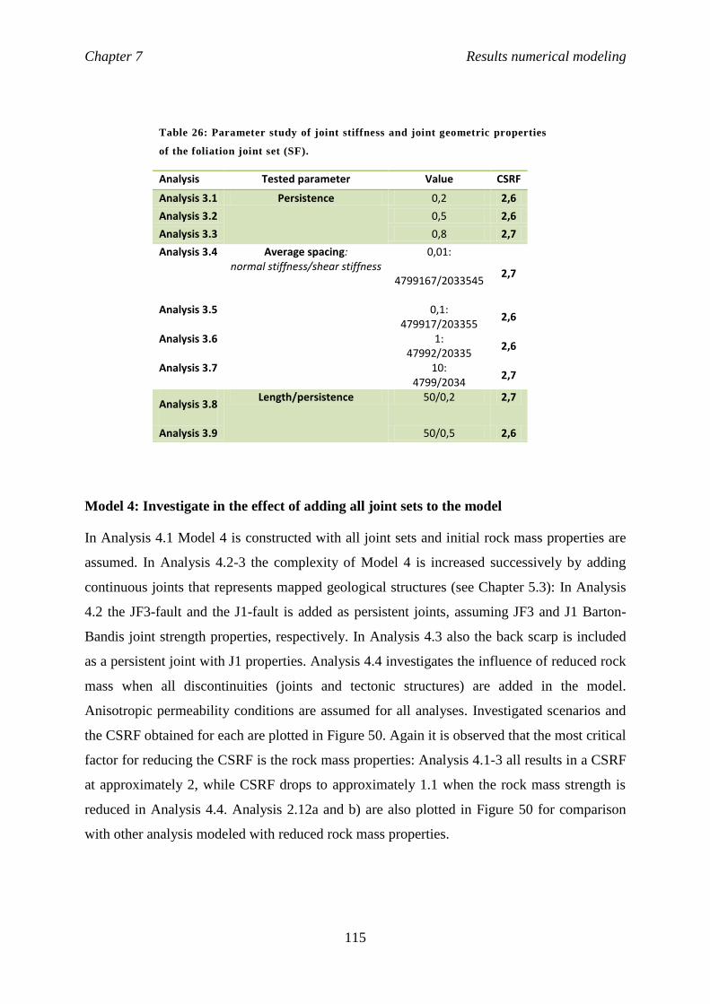
Chapter 7 Results numerical modeling
115
Model 4: Investigate in the effect of adding all joint sets to the model
In Analysis 4.1 Model 4 is constructed with all joint sets and initial rock mass properties are
assumed. In Analysis 4.2-3 the complexity of Model 4 is increased successively by adding
continuous joints that represents mapped geological structures (see Chapter 5.3): In Analysis
4.2 the JF3-fault and the J1-fault is added as persistent joints, assuming JF3 and J1 Barton-
Bandis joint strength properties, respectively. In Analysis 4.3 also the back scarp is included
as a persistent joint with J1 properties. Analysis 4.4 investigates the influence of reduced rock
mass when all discontinuities (joints and tectonic structures) are added in the model.
Anisotropic permeability conditions are assumed for all analyses. Investigated scenarios and
the CSRF obtained for each are plotted in Figure 50. Again it is observed that the most critical
factor for reducing the CSRF is the rock mass properties: Analysis 4.1-3 all results in a CSRF
at approximately 2, while CSRF drops to approximately 1.1 when the rock mass strength is
reduced in Analysis 4.4. Analysis 2.12a and b) are also plotted in Figure 50 for comparison
with other analysis modeled with reduced rock mass properties.
Table 26: Parameter study of joint stiffness and joint geometric properties
of the foliation joint set (SF).
Analysis Tested parameter Value CSRF
Analysis 3.1 Persistence 0,2 2,6
Analysis 3.2 0,5 2,6
Analysis 3.3 0,8 2,7
Analysis 3.4 Average spacing: normal stiffness/shear stiffness
0,01:
4799167/2033545 2,7
Analysis 3.5 0,1: 479917/203355
2,6
Analysis 3.6 1: 47992/20335
2,6
Analysis 3.7 10: 4799/2034
2,7
Analysis 3.8 Length/persistence 50/0,2 2,7
Analysis 3.9 50/0,5 2,6

Chapter 7 Results numerical modeling
116
The model in Analysis 4.4 has the model set up that is closest to reality, as it includes all
major geological structures that are mapped as important for the slope stability (J1, JF2, JF3,
J4, SF, back scarp, J1-fault, JF3-fault and groundwater table below the surface). A CSRF of
1.1 is obtained under the specified settings. The Maximum Shear Strain plot in Figure 51A)
indicates most significant strain concentration in the toe of the slope and in several steeply
dipping zones in the area of the model that coincide with the assumed limits of the Håkåneset
instability. In addition, a minor strain concentration area is indicated subsurface in the upper
part of the mountain slope.
Figure 50: Sensitivity study of Model 4. Investigate the effect of adding mapped geological structures
in the Model 4.
0
0,5
1
1,5
2
2,5
0 20 40 60 80
Cri
tica
l Str
en
gth
re
du
ctio
n f
acto
r
Friction angle (peak)
Sensitivity study Model 4 (all joint sets)
Initial: All joint sets. Low GW (Analysis 4.1)
Fault zone and weakness zone,low GW (Analysis 4.2)
Fault zone, weakness zone and back scarp, low GW (Analysis 4.3)
Fault zone, weakness zone and back scarp, reduced rock mass, low GW (Analysis 4.4)
Model 12a, Analysis 2.12 (J1, reduced rock mass, high GW table)
Model 12b, Analysis 2.11 (J1, reduced rock mass, low GW table)

Chapter 7 Results numerical modeling
117
A)
B)
Figure 51: Subsection of Model 4. Analysis 4.4 is the most complex model constructed in this study
and includes: All joint sets (J1, JF2, JF3, J4, SF), the back scarp, J1-fault zone, JF3-fault and the
weakness zone that intersect the profile. When 30% reduced rock mass properties (peak = 44, peak
c = 0,75) and anisotropic permeability conditions are assumed the CSRF is calculated to 1.1.

Chapter 8 Discussion
118
8 DISCUSSION
8.1 Geological investigation of the Håkåneset rockslide
8.1.1 STRUCTURAL ANALYSIS OF FIELD AND TLS-DATA
Geological site investigation of the unstable rockslope at Håkåneset, revealed that unstable
rock mass is heavily dissected by five discontinuity sets J1, JF2, JF3, J4 and SF.
Supplementary structural analysis of TLS-data in COLTOP confirms that all dominant joint
sets in the study area was mapped in field. A consistent bias between the orientations
determined by field measurements and by TLS-analysis can be explained with the overlap in
the scan direction of the TLS survey. The foliation planes of SF were not visible in the TLS-
analysis, which can be justified due to its shallow dip perpendicular to the scan direction.
J1 (075°/63°, 076°/51°) dips in the direction of the slope and has been interpreted as a
exfoliation along preexisting joints. JF2 (360°/67°, 355°/51°), JF3 (140°/78°, 138°/79°) and
J4 (207°/71°, 213°/76°) are interpreted as inherited tectonic structures that has been
gravitationally reactivated. Factors indicating that the mountain slope is heavily affected by
tectonics are:
- A persistent fault zone is a reactivated tectonic structure with JF3 orientation that cuts
through the study area. Hence, the JF3 joints can be considered as gravitational
reactivated inherited tectonic structure.
- Mineral lineations formed by muscovite sheets, observed on a JF2 surface (described
in the project assignment) support the interpretation of tectonic activity.
- JF2 and JF3 orientations fit to a conjugate strike-slip fault system that appears
regionally in Telemark.
- Joint surfaces with mineralization are dominant in the entire slope. Mineralization of
joint surfaces may occur by tectonic activity.
- The rock mass in the J1-fault zone that daylight in the road cut (at Location 6 in
Appendix 1) is dissected by lenses structure. Lenses forms by tectonic movement.
In field the foliation SF (277°/15°, 031°/16°) was observed as variable both in development
and orientation. Based on analyses of oriented thin sections of in situ rock from the road cut in
the study area a distinct foliation was identified with N-NE trend. Thus the direction of the
foliation in the lower-south domain determined in field is supported by the thin section

Chapter 8 Discussion
119
analysis. The thin section analysis confirms that foliation is defined by biotite and muscovite
sheets oriented in a preferred orientation parallel to deformed grains of other minerals in a
fine grained matrix.
J1, JF2, JF3 and J4 are all steeply dipping, and a kinematic test indicate that the orientation of
these joint sets make planar sliding, wedge sliding and toppling feasible:
1. Planar sliding is feasible in steep parts of the slope along planes of minimum dipping
values of the exfoliation plane (J1) dipping 50-65 degree in NE direction towards
Tinnsjø.
2. Wedge sliding formed by the intersection of the conjugate joint sets JF2 and JF3 is
feasible where the slope is steeper than 50-60 degrees.
3. Toppling of small blocks is feasible due to the closely spaced joint sets J4 that dips 50-
90 degrees into the slope.
The failure mechanisms described above are limited to steep slope sections only, and can only
occur for small rock volumes. This is confirmed with field observations, where significant
rock block toppling and wedges formations was observed in the road cut.
Large scale rock slope deformation can only be justified by assuming deformation along a
combination of several anisotropies. J1 and SF have been considered as the most critical joint
sets to make massive slope feasible:
1. Because J1 is steeply dipping (50-65 degree) and SF is shallowly dipping (up to 19
degree) and both with the approximately same dip direction towards NE they can form
a compound sliding surface characterized as bi-planar sliding.
2. A possible back scarp and a weakness zone formed by tectonic activity are oriented
like J1.
3. Mineral lineations and groove marks were observed in field on a J1 surface. These are
indicators of displacement along J1, even though their presence is not statistically
significant.
4. Thin section analysis indicates that microfracturing is strongly affected and develops
parallel to the foliation (not statistically significant).
Due to prominent subaquatic bedrock structures on the bathymetric map (see Figure 21) it is
considered reasonable to assume the same rock mass characteristics in the subaquatic
component of the instability as in the subaerial. A distinct cut off in the relief of the
bathymetric structures is interpreted as evidence that the two distinct SW-NE striking faults in

Chapter 8 Discussion
120
the central part of the studied area form the northern lateral release surface of the Håkåneset
rock slide. Such clear release surface does not occur in the south and the bathymetric data
rather suggest that the limit of the unstable area in the south is transitional. No systematic
decrease of degree of damage of the rock mass towards the south in the subaerial slope
component can be interpreted as an indication that the fracturing of the rock mass mainly
have taken place before an assumed sliding process started. This is also supported by the fact
that the orientations of all joint sets appear consistent also outside the defined lateral limits of
the instability. According to Stead and Eberhardt (2013) is release surfaces an essential
component of kinematic release for a landslide. Obviously, the missing distinct lateral limit in
the south is a factor that reduces the likelihood of a massive failure of the slope. The buttress
observed in the bathymetric image in the south of the study area can be the sufficient
stabilizing feature that has prevented a southern lateral limit to be developed.
8.1.1 RECORDED SLOPE DEFORMATION ACTIVITY
SW movement trend in the differential GNSS analysis is consistent with the direction of
toppling failure along J4. Notwithstanding, the dGNSS measurement is based on only one
year's interval and from one rover point only, thus being far from statistically significant. The
annual scale rate (9 mm horizontally and 2 mm vertically) is however supported by traditional
GPS displacement measurements undertaken by SSV from 2003 to 2006 that revealed an
annual average displacement of 10 mm horizontally and 2 mm vertically in at the exposed
location called Gvålvikknatten in the central area of the Håkåneset rockslide (see Appendix
1). In both of the geodetic measurement approaches that have been undertaken the horizontal
displacement is higher than the vertical. According to Wyllie and Mah (2004) is horizontal
displacements greater than vertical displacements characteristics for toppling behavior. This
support that the small scale displacements that are recorded can geologically be explained as
toppling activity of smaller rock volumes.
The displacement analysis performed on TLS-data did not reveal any reliable results due to
limited quality of the data set. However, frequent rock fall recorded along the road by SVV
(see also Figure 8 and Figure 9) can be interpreted as evidence that there are activity in the
slope due to large slope deformation. Although this is true, external factors like road
construction effects, erosion, freeze and thawing etc. will likely be a significant factor for
triggering rock fall.

Chapter 8 Discussion
121
8.1.2 FINDINGS FROM SSR-ANALYSIS
Impact of topography on slope stability
Stead and Eberhardt (2013) mention tension cracking in the slope crest and heave/bulging at
the toe as early indicators of slope instability, where slope topography is one of the essential
factors controlling the spatial distribution of such damages in a rock slope. The analysis result
presented in this study (Chapter 7) seem to indicate that the topography is a vital factor also
for the presence of the Håkåneset instability, because active zones in the maximum shear
strain plots area are concentrated in majority in the toe of the slope model and in a smaller
area in the upper region in the mountain slope for all analyses. Since the topography in the
model is the only factor that is kept constant in all analyses, its importance as a dominating
factor to the strain concentration is justified.
The induces active zone in the toe is also clearly seen on displacement contour plots that
indicate that most significant displacement out of the slope can be expected at approximately
100 m depth in Lake Tinnsjø. This is supported by prominent geological structures on
bathymetric map. The buttress in the south of the study area is located at approximately the
same elevation as the indicated active zone, and strengthens the assumption of the buttress
being a vital stabilizing feature.
Sensitivity of hydrogeological conditions
According to Wyllie and Mah (2004) there are in particular two essential water pressure
properties that reduces stability: 1) the diminishing of the shear strength of potential failure
surfaces and 2) increasing the forces that induce sliding when present in tension cracks and
near vertical fissures.
A subsurface groundwater table was obtained from the groundwater seepage analyses when
anisotropic permeability with vertical permeability significantly greater than the horizontal
permeability was assumed. Because the rock mass at Håkåneset is heavily dissected by
steeply dipping joint sets (> 50 degree for both J1, JF2, JF3 and J4) this anisotropic
permeability condition is assumed as realistic. By assuming isotropic permeability in the
material the groundwater seepage analysis resulted in a surface near groundwater table.
According to Wyllie and Mah (2004) can a surface parallel groundwater table in strong rock
with widely spaced joints be justified by the fact that the a low porosity rock imply that the

Chapter 8 Discussion
122
water flow will rapidly fill the joints close to surface and increase the water pressure in the
slope in periods of increased precipitation. Therefore, in order to take account for periods of
heavy rain fall and snow melt as a worst case scenario a surface near groundwater table can be
assumed realistic to use in a numerical modeling.
Obviously, a lower groundwater table will have a positive effect on the CSRF due to
increased effective stresses when the pore pressure decreases, which is confirmed in Analysis
1.1_2 (Figure 34) and Analysis 1.1_3 (Figure 35) and illustrated in Figure 38. However, by
studying Figure 50 it is seen that the outcome of this analyses indicates that the sensitivity of
slope stability to groundwater table location under the defined hydraulic conditions is
negligible compared to the effect of varying the material properties. The importance of
material properties to slope stability is discussed in the next section.
Excluding the constructed lake water (pounded water and water load) in the Model 1 had no
effect on the predicted CSRF, as can be seen from the result of Analysis 1.3 and 1.1_3. Also
the maximum shear strain contours for each analysis, Figure 36 and Figure 37 respectively,
were only slightly changed. This can be interpreted as an indication that the stabilizing effect
of a water load from the lake is negligible compared to the major effect of the topography to
induce unstable areas in the Håkåneset mountain slope. On the contrary, it is well known that
the presence of groundwater and the associated water pressure on a potential sliding plane is
crucial in rock slope stability (Nilsen et al., 2000). Therefore, the lack of sensitivity in the
model by excluding such an essential factor as the water highlights the importance of
interpreting numerical modeling results with caution. Essential hydrogeological factors and
their effect on the stability of the Håkåneset rockslide are further discussed in Chapter 9.3.
Material strength as a controlling factor for massive slope failure
The numerical modeling undertaken in this study highlights the rock mass strength as the
most critical factor to slope stability. This is experienced both from the sensitivity study of
Model 1, 2 and 4 where CSRF is significantly changed when rock mass parameters are varied,
as illustrated by the plots in Figure 38 and Figure 50. Figure 38 shows the results obtained by
sensitivity test with Model 1 (J1 joints included as the only discontinuities), where it is clear
that the rock mass strength is the fare most controlling factor in comparison the other tested
factors, i.e. the groundwater level. From Figure 50 it become visible that the dominance of the
rock mass strength as the controlling factor to slope stability also is supported by the

Chapter 8 Discussion
123
sensitivity study of Model 4. Realistically, Model 4 should represent a more unstable slope
than Model 1-3 since the material is broken up by the discontinuities that represent the rear
release surfaces. Still, the CSRF appears not to be affected by the discontinuities and is only
changed significantly when the rock mass strength is reduced.
The vital importance of rock mass strength to rock slope stability is easily justified by the fact
that the joint sets at Håkåneset are non-persistent, implying that damage of intact rock is
necessary in the development of a basal sliding surface. A basal sliding plane is an essential
structure in a rockslide. Bjerrum (1967) defines progressive failure as the process where a
continuous sliding surface is developed by damage of intact material. Furthermore, Eberhardt
et al. (2004) justify degradation of rock mass strength as the vital factor for progressive failure
in a natural rock slope. Progressive failure and degradation means that the rock mass strength
is reduced over time due to the propagation of fractures through intact rock between existing
discontinuities. Obviously, this damage controlled failure mechanism is developed by a
through-going step path failure, involving tension failure by microcracking and shear failure
of intact rock (Stead and Eberhardt, 2013). The foliation parallel microfractures seen in thin
the sections of insitu rock from the study area can be used as supporting indicators of
progressive failure.
Terzaghi (1962) emphasize that shear failure is controlled by two parameters:1) the shearing
resistance represented by the friction angle (φ) and 2) the cohesion (c) of intact rock bridges
between discontinuous joints. The sensitivity test results of friction angle and cohesion
undertaken in this study, plotted in Figure 44, indicate that the stability of the slope is most
sensitive to changes in friction angle. Slope stability is quantified by the CSRF, which by
definition depends on the shear strength. When shear strength is plotted to percentage value
reduction of friction angle and cohesion separately, see Figure 46, the same trend with shear
strength being more sensitive to changes of friction angle than changes of cohesion, is
observed. Analysis 2.12 investigates how friction angle and cohesion influences the slope
differently for a specific CSRF condition. Figure 46A illustrate the reduction of friction angle,
indicating that the J1 discontinuity is important due to the distribution of the strain
concentrations. In Figure 46B) on the other hand, is the cohesion reduced, and J1 seems to be
less important as the strain concentration appears in a smaller region but with higher
magnitude of the maximum induced strain. The result of Analysis 2.12 indicates that the
strain concentration in the slope is significantly affected by the magnitude of friction angle
relative to the cohesion. A possible explanation to this observation is: Because the cohesion is

Chapter 8 Discussion
124
related to the shearing of intact rock in rock bridges it is reasonable to assume that rock
damage becomes easier when the cohesion is reduced, implying that more rock bridges in a
smaller area can be sheared. The friction angle is related to the frictional restrain in the rock,
and consequently sliding along J1 surfaces can be assumed to be easier when friction angle is
reduced. To summarize, when the rock is less cohesive the development of a failure surface is
less affected by pre-existing joints because rock bridges between sub parallel joints are more
easily shared, while for a rock with reduced friction angle the weakness defined by pre-
existing joint become even more pronounced because the strength contrast between the joint
and the rock bridges become even stronger. The J1-fault and the J3-fault are mapped out with
as with a persistence in the km scale and have several indicators suggesting they are essential
for the development of the instability in the Håkåneset rockslope. Both of these structures
have orientations that correspond to a joint set. In addition, the interpreted back scarp, which
is the third persistent structure that is essential for the slope stability, also has a orientation the
correspond to a existing joint set (J1). The fact that the persistent faults and the back scarp are
developed along pre-existing joints, suggest that the model that strengthens the importance of
the joints in the model, i.e. a model with a frictional angle reduce compared to the initial
value, best describes the reality.
The role of the J1 discontinuity set on the slope stability
As discussed above does the result from the rock mass sensitivity test in Analysis 2.12
highlight the pre-existing joints as essential for the stability in the slope. As described in
Chapter 9.1.1. is the exfoliation joint set J1 considered as vital for the slope stability due to
field observations and its control on the kinematics of the rockslide. In the FEM-analysis the
importance of J1 regarding slope stability was first confirmed by adding J1 as ubiquitous
joints in Analysis 1.6, where the resulting Safety Factor plot, Figure 42A, indicate most
critical parts in the region of the model where the instability is located in nature. Active zones
indicated with ubiquitous joints have also been justified by Böhme et al. (2013) for the
Stampa rockslide in western Norway. Adding J1 to the Phase2
model as a joint network in
Analysis 2.1 did not change the CSRF value, but had a significant effect on where strain
concentrations were induced: with J1 joints in the model several steeply dipping strain
concentration zones parallel to the orientation of J1 joints became dominant. These strain
concentrations were induced mainly in the lower part of the constructed mountain slope and
fit well to the where the back scarp and the fault zones would intersect the profile that the

Chapter 8 Discussion
125
model in constructed from. The trend of back scarp and the fault zones in the profile can be
seen on Figure 54. These observations clearly highlight the importance of the J1 joint set as a
crucial structure for the stability of the rock slope at Håkåneset.
The J1-fault and the back scarp is interpreted as two possible rear release surfaces. As
mentioned, adding J1 in the model indicates several steeply dipping strain concentrations with
J1 orientation. With this observation, the feasibility for the development of new rear release
surfaces in addition to J1-fault and the back scarp cannot be excluded. The varying
topography and graben morphology in the upper part of the slope are observations that
support that several more active sliding zones are present in the deforming rock slope.
However, in case of a basal failure surface is developed and allow for sliding it would be
reasonable to think that the back scarp and fault zones would be critical as rear release
surfaces because of their persistent character and reduced strength due to earlier damage.
With this, the importance of the exfoliation joint set regarding the stability of the Håkåneset
rockslide is clearly supported by the results from the undertaken numerical modeling in this
study.
The role of the foliation on the slope stability
By field observations and kinematic feasibility test, the foliation joint set SF was identified as
important for the formation of a basal sliding surface. By numerical modeling this
interpretation was first supported when most active zones corresponding to the instability
came out clearly in the ubiquitous joint strength factor plot of Model 1, as illustrated in Figure
42B. By comparing Figure 42A and Figure 42B it can be observed that a larger of area of the
instability in the Håkåneset rock slope is indicated as critical in the plot when SF is included
(Figure 42B). This strengthens the importance of SF to the instability of the slope.
Furthermore, was SF included in Phase2 model as a joint network of non-persistent joints,
defined with shorter length and less persistent than J1 (see Model 3 Appendix (??). As
observed when J1 was included in the modeling, adding SF did not have any effect on the
CSRF either. The shear strain contours plots for Model 2 and Model 3, given in Appendix ??,
indicate only minor differences. Still, with SF present in the model the strain concentrations
seem to appear more distinct, and a likely basal sliding plane is reasonable to interpret to
develop with SF direction, daylighting at approximately 100m depth in Lake Tinnsjø. On the
contrary, the mean dip angle of SF (19°) is less than the assumed friction angle of the

Chapter 8 Discussion
126
discontinuities (28°), thus sliding along foliation planes alone is unlikely. This supports the
interpretation of a retrogressive step path failure as the most likely failure mechanism in the
development of a basal sliding surface for the Håkåneset rockslide. In the field were the
foliation planes mapped out as purely developed, which further supports progressive failure as
failure mechanism. Identified microfracturing parallel to the foliation in thin sections of the
insitu rock can also be used to justify the likelihood of stepped failure along foliation joints.
With this, the development of a basal sliding plane have to be assumed to require significant
rock damage, thus confirming the previous interpretation of the rock mass as the most
controlling factor for this instability. The lack of sensitivity in the modeling when varying
important joint parameters like persistence, spacing and stiffness, as seen from the results
presented in Table 26 can be justified with the dominance of rock mass strength in the
development of a sliding surface.

Chapter 8 Discussion
127
8.2 Influence of Lake Tinnsjø on the stability of the Håkåneset
rockslide
In particular two important factors are evaluated as essential regarding the presence of Lake
Tinnsjø and the instability at Håkåneset: 1) the stabilizing effect due to hydraulic pressure
from the water column and 2) the depth of the groundwater table on which the induced pore
water pressure in the rock masses is strongly dependent. Some reflections regarding these
effects are discussed in the following text. In addition, a buoyancy effect must be expected to
influence on the stability in a negative way, as seen in the study of the Hochmais–Atemkopf
rockslide by Schneider-Muntau and Zangerl (2005)
Following the definition given by Born et al. (1979) Lake Tinnsjø can be classified as a
discharge lake due to its location with respect to the surrounding topography. The
groundwater table in this environment will always communicates with the lake level and
raises close to the surface along the mountain slope as seen in Figure 52. In a temperate
climate like in southern Norway, precipitation and consequently the groundwater table level is
variable. Figure 53 illustrates how a fluctuation of the groundwater table due to variable
precipitation periods will affect a combined subaerial-subaquatic rock slope instability
differently than a fully subaerial instability. The fact that the groundwater table always will
communicate with the lake surface implies that the groundwater table variations only will
affect the upper part of the instability, while for the subaerial rockslope the hydrogeological
conditions in the unstable rock mass can change from almost dry to fully saturated conditions.
Based on this it should be reasonable to expect that lake Tinnsjø is favorable as regards
stabilizing the deforming rock mass at Håkåneset because its presents contribute to less
variations in the groundwater table, and consequently negative effects due to induces seepage
forces is prevented. This interpretation is however strongly dependent on that the lake surface
level can be constant, so that seepage forces due to a fluctuating lake level can be considered
as negligible.

Chapter 8 Discussion
128
Figure 52: Typical groundwater flow (black arrows) in a discharge lake like
Tinnsjø. The groundwater table (dotted line) communicate with the lake level and
raises subsurface along the mountain slope (Born et al., 1979)
a)
b)
Figure 53: General groundwater condition for a rock slope instability that has a) a subaerial and a
subaquatic component and b)only a subaerial component (modified from Wyllie and Mah (2004)).

Chapter 8 Discussion
129
8.3 Volume estimation of the deforming mass in the Håkåneset
rockslide
Figure 54 show the result from Analysis 4.4 on Model 4 and illustrate the location of the
failure surface that is interpreted as most likely due to the numerical modelling obtained in
this study. Justification of the interpretation is given in the following text.
A bi-planar failure mechanism is interpreted as likely for the Håkåneset rock slope. Model 4
is the model in this study that is constructed to reflect the most of the actual structures in the
slope. In Analysis 4.4 a condition close to the critical state (CSRF ~ 1) obtained in, thus the
contour plots from this analysis is reasonable to use for indication of the failure surface in
case of a massive slope failure.
The failure plane is interpreted to be compound of 1) a steep rear release surface developed
along J1 joints and 2) a shallow basal failure surface developed by retrogressive failure along
the schistose foliation. These interpretations are based on visual analysis of shear strain and
displacement contour plots. The reliability of the results can be justified due to the fact that:
a. the location of the most active zones is approximately consistent for all analyses.
b. the active zones are indicated in areas of the model that coincide with the location
geological structures (back scarp, two fault zones) that was interpreted as important
for the slope stability during the geological investigation.
c. the interpreted basal sliding plane daylight the slope at a location that coincide with a
topographic step in the topography. This step may be interpreted as a bulging toe.
According to Stead and Eberhardt (2013) is a bulging toe considered as a pre-indicator
of slope instability.
Due to the persistent character of the mapped back scarp and the J1-fault zone these are
considered to define the most likely rear release surfaces. In addition, during the field
investigation the material in the J1-fault zone was observed as significantly disturbed and
with clay content. Based on this it is reasonable to assume that the shear strength along the J1-
fault is significantly reduced compared to other J1-joints. These observations support a
scenario with the J1-fault as rear release surface in combination with the basal sliding plane
daylighting at approximately 100 meters depth in Lake Tinnsjø. Worst case scenario is
induced if failure takes place along the back scarp.
The geometry the Phase2 profile in Figure 54 of each of the rear release surface scenarios
described above is used for the volume calculation. The extend of the instability at surface

Chapter 8 Discussion
130
was estimated in ArcMap 10.1 (Esri, 2012). Because the southern limit of the rockslide is
assumed to be translational, two scenarios were calculated: 1) the buttress limits the instability
and 2) the topographic gully is the limit (worst case). The calculations are given in Appendix.
Assuming the J1-fault as rear release predict a deforming volume from 17 to 33 million m3 if
the southern limit controlled by the buttress or the gulley, respectively. Worst case scenarios
with the back scarp are rear release surface predict that the instability involves a rock mass in
the range of 74 to 144 million m3.
From the conclusions about the effect of Tinnsjø on the slope stability, it is interesting to
consider a cenari where the basal surface daylights at the lake level, where hydrostatic
pressure from the lake is not effecting the slope. Under these conditions the unstable mass is
estimated to be in the range from 2 - 4 million m3 with J1-falt as release surface and 26-50
with the back scarp as rear release surface.

Chapter 8 Discussion
131
A)
B)
Figure 54: A) Maximum shear strain and B) Total displacement in Model 4, Analysis
4.4. A compound sliding surface is indicated (red dotted) by visual interpretation.

Chapter 8 Discussion
132
8.4 Uncertainties in the slope stability assessment of Håkåneset
rockslide
In this slope stability assessment of the Håkåneset rockslide several techniques are applied,
which require a great amount of input parameters. The quality of modeling results is
impossibly better than the input parameters. Obtaining representative values for the required
parameters on which the modeling is based is challenging and the result can never be
concluded as completely true. In addition are significant simplifications of the reality
necessary when constructing the model. While this is true, when the modeling results show
reasonable patterns that can be related to observations in the field the reliability of the model
is increased. Because of this possibility of visual justification numerical modeling is well
accepted as an efficient tool in slope stability assessment for getting an impression of what
can be considered as most likely critical factors and conditions. Several of the obtained results
for this study of the Håkåneset rockslide can be justified with field observations, which adds
reliability to the constructed model. However, it is important to be aware of the most
important limitations and uncertainties related to the undertaken stability assessment. This
will be discussed in the following text.
By nature geology is complex and anisotropic, thus the isotropic rock mass assumption which
the numerical modeling is bases on is unrealistic.
Induced stresses and the resulting strains depend on the field stress in the rock mass, thus the
strain contour plots obtained in the numerical model should realistically be dependent on the
defined stress field. The stress field values used as input in this study are empirical values,
which means their representativeness for the in situ conditions at Håkåneset is questionable.
Nonetheless, since Phase2 is a 2D-program it is difficult to obtain stress distribution
parameters that take into account the natural three dimensional stress fields. While this is true,
in the case of the undertaken modeling the reliability of the assumed field stress can be
justified because the shear strain patters obtained by the undertaken modeling can be related
to major structures mapped in the field and on the DEM. In addition, experience from
previous rockslope stability studies indicate that field stress only have minor influence on the
SSR analysis (Loftesnes, 2010; Sandøy, 2012).

Chapter 8 Discussion
133
The results from the undertaken numerical modeling highlight the rock mass strength
parameters (friction angle and cohesion) as a critical factor for driving the slope towards a
disequilibrium conditions.
Estimations for the rock parameters in this study are obtained by field and laboratory results
on in situ rock. Representative rock samples are in general difficult to obtain. The rock
samples used in this study were collected from the road cut and were partly detached, thus
their representativeness for intact in situ rock is highly questionable as strength reduction due
to the influence from the road construction might be significant. The uncertainty related to the
rock strength is further supported by the unrealistic relationship with the laboratory estimate
for UCS as lower than the field estimate for JCS. In addition, significant uncertainties related
to scale effect when obtaining rock properties with different approaches will always be
present even though the scale are accounted for by empirical based conversions.
The numerical setup requires initial rock mass input parameters for friction angle and
cohesion determined as instantaneous strength parameters under an assumed normal stress
condition. The normal stress condition is determined by assuming that the basal failure
surface develops in rock mass with 100 m overburden. The location of a possible basal plane
for a massive failure of the Håkåneset rockslide is unknown, thus the assumed overburden of
100 m is a major simplification of the reality and add uncertainty to the modeling. In addition,
since the predicted failure plane geometry of the Håkåneset rockslide is bi-planar and due to
topography, the overburden of the failure surface will be variable, implying that normal stress
level and consequently the rock mass strength also will be variable.
Retrogressive failure is concluded as the most likely failure mechanism for the Håkåneset
rock slope. This mechanism involves tension cracking, thus the tensile strength of the rock
will be essential in the development of the sliding plane. In the undertaken numerical
parameter study the significance of the tensile strength due to strain concentrations have not
been tested for, which is an important limitation of the undertaken parameter study
The importance of joint spacing and persistence on rock slope kinematics are well
documented, e.g. by (Brideau et al., 2008). Still, the performed parameter study of SF joints in
the model had negligible effect on the safety factor and strain estimation. This is not realistic
and is a significant limitation of the numerical model in this study. A possible explanation to
the lack of influence might be that because the joints are constructed to be non-persistent the

Chapter 8 Discussion
134
importance of rock mass properties masks the influence of varying joint characteristics. Also,
the dominant topographic effect might contribute to this.
Because the Håkåneset rockslide extends both over and under water and a groundwater table
will naturally be an essential component to include in the model. In addition, the rockslide is
located in a climate region where frequent rainy periods are common, thus a fluctuation
groundwater table and induced seepage forces will be part of the reality. Seepage forces has
not been taken into account in this study, neither have infiltration conditions. Water
conditions are complex and introduce significant uncertainties and limitations to the
modeling. Some important uncertainties related to the Håkåneset modeling are:
- seepage forces and infiltration conditions
- the permeability of the rock mass
- the hydrogeological conditions of joints
- the influence of the fault to the groundwater table location
A detailed description of groundwater conditions related to slope stability is given by Wyllie
and Mah (2004).

Chapter 8 Discussion
135
8.5 Recommendations for further investigations
Based on the described uncertainties regarding both geological factors and hydrological
conditions there is still need for increased knowledge about the Håkåneset rock slide. In
particular it is important to obtain better dataset to detect the ongoing deformation. Therefore,
it is important that dGNSS measurements are continued for several years in order more
comparable data. The measurements should be optimized by installing additional rover points
in order to detect whether the observed displacement is a result of massive slope deformation
or minor scale block toppling. Also, to continue to with the TLS survey is considered
important for detecting rock fall activity. For further TLS surveys it must be emphasized to
focus on increasing the quality of the data, as the data set used in this study was not sufficient
to obtain reliable results.
The numerical modeling suggests the J1-fault as a likely rear release surface, and obtaining
more reliable material strength properties for this zone would be important for further
predicting the likelihood of sliding along this zone. Test material can be easily obtained, since
this structure is daylighting in the road cut. Shear box test can be used to determining the
shear strength of such weakness zone material. In the field clay filling on discontinuities
surfaces within the damaged rock mass in this weakness zone was observed. It is
recommended that this material is tested for swelling clay, because swelling effect is a critical
phenomenon regarding rock stability. Identification of swelling clays can be obtained with a
X-ray diffraction (XRD) analysis in the laboratory of NTNU/SINTEF.

Chapter 8 Discussion
136
Chapter 9 Conclusion
137
9 CONCLUSION OF THE STUDY
Structural analysis on TLS data validated the previously obtained structural field
measurements and the kinematical model of the Håkåneset rock slide. The undertaken FE-
SSR analysis in Phase2 supports that bi-planar failure mechanism involving development of a
basal failure surface by retrogressive failure is feasible.
The stability assessment suggests that:
The steeply dipping exfoliation joint set (J1 (075°/63°, 076°/51°)) can be confirmed
essential for defining a rear release surface. A fault and a back scarp visible in the
subaerial slope are persistent structures with J1 orientation that justify the importance
of J1 in case of a massive slope failure. The presence of multiple sliding surfaces is
supported by strain concentration contours obtained by numerical modeling, and can
also be justified by the variable topography in the rock slope.
Due to topographic influence it is reasonable to expect that the most active zone is in
the submerged part of the slope even though hydrostatic forces from the lake will act
as a stabilizing factor. This is justified by prominent bedrock structures on bathymetric
map. Visual analysis of strain concentrations plot suggests that a basal failure surface
can daylight at approximately 100 m depth in the lake. In addition this adds reliability
to the interpretation of a subaquatic buttress being a significant stabilizing factor and
the reason for the lack of a clear southern lateral limit.
A basal failure surface can be developed by step-path retrogressive failure. This
requires significant rock damage, as the field observations indicate that schistose
foliation planes are poorly developed. Thin section analysis revealed that the rock is
strongly anisotropic and have indicators that justify shear deformation, which supports
that development of a basal sliding surface is feasible.
With retrogressive failure as a likely failure mechanism, the rock mass shear strength
properties are crucial to investigate to predict the likelihood of large scale failure to
occur.
Volumes in the range 2 - 50 million m3 is estimated for failure involving only
subaerial material, and 17-144 million m3 if the basal failure surface is assumed to
daylight at the submerged toe. These calculations are indeed very uncertain and further
stability assessment of the Håkåneset rockslope is highly recommended before
predicting the likelihood of a massive failure of the slope.

Chapter 9 Conclusion
138
Chapter 10 References
139
10 REFERENCES
Revista de la Asociación Geológica Argentina: Buenos Aires, Asociación Geológica
Argentina.
Abellán, A., Oppikofer, T., Jaboyedoff, M., Rosser, N. J., Lim, M., and Lato, M. J., 2014,
Terrestrial laser scanning of rock slope instabilities: Earth Surface Processes and
Landforms, v. 39, no. 1, p. 80-97.
Atkinson, L. C., 2000, The role and mitigation of groundwater in slope stability: Slope
Stability in Surface Mining, p. 89.
atlas.nve.no, The National Catchment Database (REGINE), Volume 2014, Norwegian Water
Resources and Energy Directorate
Bandis, S., Lumsden, A., and Barton, N., Fundamentals of rock joint deformation, in
Proceedings International Journal of Rock Mechanics and Mining Sciences &
Geomechanics Abstracts1983, Volume 20, Elsevier, p. 249-268.
Barton, N., 1973, Review of a new shear-strength criterion for rock joints: Engineering
geology, v. 7, no. 4, p. 287-332.
Barton, N., and Choubey, V., 1977, The shear strength of rock joints in theory and practice:
Rock mechanics, v. 10, no. 1-2, p. 1-54.
Bitelli, G., Dubbini, M., and Zanutta, A., 2004, Terrestrial laser scanning and digital
photogrammetry techniques to monitor landslide bodies: International Archives of
Photogrammetry, Remote Sensing and Spatial Information Sciences, v. 35, no. Part B
5, p. 246-251.
Bjerrum, L., 1967, Progressive failure in slopes of overconsolidated plastic clay and clay
shales: Journal of Soil Mechanics & Foundations Div.
Blikra, L., Longva, O., Braathen, A., Anda, E., Dehls, J., and Stalsberg, K., 2006, Rock slope
failures in Norwegian fjord areas: examples, spatial distribution and temporal pattern,
Landslides from massive rock slope failure, Springer, p. 475-496.
Born, S., Smith, S., and Stephenson, D., 1979, Hydrogeology of glacial-terrain lakes, with
management and planning applications: Journal of Hydrology, v. 43, no. 1, p. 7-43.
Brideau, M.-A., Yan, M., and Stead, D., 2008, The role of tectonic damage and brittle rock
fracture in the development of large rock slope failures: Geomorphology, v. 103, no.
1, p. 30-49.
Bunkholt, H., Nordahl, B., Hermanns, R. L., Oppikofer, T., Fischer, L., Blikra, L. H., Anda,
E., Dahle, H., and Sætre, S., 2013, Database of unstable rock slopes of Norway.: In:
Margottini C, Canuti P, Sassa K (eds) Landslide science and practice, Springer,
Berlin, v. 3, no. Spatial analysis and modelling., p. 423-428.
Böhme, M., Hermanns, R. L., Oppikofer, T., Fischer, L., Bunkholt, H. S., Eiken, T.,
Pedrazzini, A., Derron, M.-H., Jaboyedoff, M., and Blikra, L. H., 2013, Analyzing
complex rock slope deformation at Stampa, western Norway, by integrating
geomorphology, kinematics and numerical modeling: Engineering Geology, v. 154, p.
116-130.

Chapter 10 References
140
Dons, J. A., and Jorde, K., 1978, Berggrunnskart Skien: Norges geologiske undersøkelse
(NGU), scale 1:250000.
Eberhardt, E., Stead, D., and Coggan, J., 2004, Numerical analysis of initiation and
progressive failure in natural rock slopes—the 1991 Randa rockslide: International
Journal of Rock Mechanics and Mining Sciences, v. 41, no. 1, p. 69-87.
Eiken, T., 2013, Deformasjonsmålingar i potensielle fjellskred, Telemark: Institutt for geofag,
Universitetet i Oslo.
Eilertsen, R., 2013, Personal communaication, Bathymetric data Tinnsjø.
Esri, 2012, ArcGIS ArcMap, Esri
Frisvold, T., 2006, Gvålviknatten rasovervåkningsprosjekt, Tinn kommune 2002/2003.
-, 2007, Gvålviknatten rasovervåkningsprosjekt, Tinn kommune. 2006.
geo.ngu.no, Nasjonal berggrunnsdatabase, Berggrunn N250 med fjellskygge, Volume 2104:
Kontaktadresse: Postboks 6315 Sluppen, 7491, The Norwegian Geological Survey.
Goodman, R. E., Taylor, R. L., and Brekke, T. L., 1968, A model for the mechanics of jointed
rock: Journal of Soil Mechanics & Foundations Div.
Griffiths, D., and Lane, P., 1999, Slope stability analysis by finite elements: Geotechnique, v.
49, no. 3, p. 387-403.
Gruber, S., and Haeberli, W., 2007, Permafrost in steep bedrock slopes and its
temperature‐related destabilization following climate change: Journal of Geophysical
Research: Earth Surface (2003–2012), v. 112, no. F2.
Grøneng, G., and Nilsen, B., 2009, Procedure for determining input parameters for Barton-
Bandis joint shear strength formulation, Trondheim, Instituttet, NTH, 21 bl. :
Grøneng, G., Nilsen, B., and Sandven, R., 2009, Shear strength estimation for Åknes sliding
area in western Norway: International Journal of Rock Mechanics and Mining
Sciences, v. 46, no. 3, p. 479-488.
Hammah, R., Yacoub, T., Corkum, B., and Curran, J., The practical modelling of
discontinuous rock masses with finite element analysis, in Proceedings Proceedings of
the 42nd US Rock Mechanics Symposium–2nd US-Canada Rock Mechanics
Symposium, San Francisco, US2008.
Hammah, R., Yacoub, T., Corkum, B., Wibowo, F., and Curran, J., Analysis of blocky rock
slopes with finite element shear strength reduction analysis, in Proceedings
Proceedings of the 1st Canada-US Rock Mechanics Symposium2007, p. 329-334.
Hammah, R. E., Curran, J. H., Yacoub, T., and Corkum, B., Stability analysis of rock slopes
using the finite element method, in Proceedings Proceedings of the ISRM regional
symposium EUROCK2004.
Hanssen, T. H. D. I., 1998, Rock stresses and tectonic activity: Fjellsprengnigskonferansen,
Oslo 1998, no. Norsk Jord- og Fjellteknisk forbund, p. 29.29 - 29.10.
Harbitz, C., Pedersen, G., and Gjevik, B., 1993, Numerical simulations of large water waves
due to landslides: Journal of Hydraulic Engineering, v. 119, no. 12, p. 1325-1342.
Hermanns, R., Hansen, L., Sletten, K., Böhme, M., Bunkholt, H., Dehls, J., Eilertsen, R.,
Fischer, L., L’Heureux, J., and Høgaas, F., 2012a, Systematic geological mapping for
landslide understanding in the Norwegian context: Landslide and engineered slopes:

Chapter 10 References
141
protecting society through improved understanding. Taylor & Francis Group, London,
p. 265-271.
Hermanns, R., and Longva, O., 2012, Rapid rock-slope failures: Landslides (types,
mechanisms and modeling). Cambridge University Press, Cambridge, p. 59-70.
Hermanns, R., Oppikofer, T., Anda, E., Blikra, L., Böhme, M., Bunkholt, H., Crosta, G.,
Dahle, H., Devoli, G., Fischer, L., Jaboyedoff, M., Loew, S., Sætre, S., and Yugsi
Molina, F., 2013, Hazard and Risk Classification for Large Unstable Rock Slopes in
Norway: Italian journal of engineering geology and environment.
Hermanns, R. L., Oppikofer, T., Anda, E., Blikra, L. H., Böhme, M., Bunkholt, H., Crosta, G.
B., Dahle, H., Devoli, G., Fischer, L., Jaboyedoff, M., Loew, S., Sætre, S., and
Molina, F. Y., 2012b, Recommended hazard and risk classification system for large
unstable rock slopes in Norway: Norwegian Water and Energy Directorate (NVE).
Hermanns, R. L., Oppikofer, T., Molina, F. Y., Dehls, J., and Böhme, M., 2014, Approach for
Systematic Rockslide Mapping of Unstable Rock Slopes
in Norway: Springer, v. 3, no.
, p. 129-134.
Hoek, E., 1983, Strength of jointed rock masses: Geotechnique, v. 33, no. 3, p. 187-223.
Hoek, E., 2007, Practical Rock Engineering, Rock Mass Properties: Toronto, Ontario,
Canada, Rocscience Inc.
Hoek, E., and Brown, E., 1997, Practical estimates of rock mass strength: International
Journal of Rock Mechanics and Mining Sciences, v. 34, no. 8, p. 1165-1186.
Hoek, E., Carranza-Torres, C., and Corkum, B., 2002, Hoek-Brown failure criterion-2002
edition: Proceedings of NARMS-Tac, p. 267-273.
Holtedahl, O., and Andersen, B. G., 1960, Glacial map of Norway: The Norwegian
Geological Survey (NGU)
scale 1:2000000.
http://www.nve.no/, The National Lake Database (Innsjødatabasen), Volume 2014:
Middelthunsgate 29, Postboks 5091 Majorstua, 0301 Oslo Norwegian Water
Resources and Energy Directorate.
Hungr, O., Leroueil, S., and Picarelli, L., 2012, The Varnes classification of landslide types,
an update: Landslides, p. 1-28.
InnovMetric, 2014, PolyWorks: 3D scanner and 3D digitizer software, InnovMetric Software
Inc.
ISRM, 2007, Suggested Methods for Determining the Uniaxial Compressive Strength and
Deformability of Rock Materials in: Ulusay, R., Hudson, J.A. (Eds.), The Complete
ISRM Suggested Methods for Rock Characterization, Testing
and Monitoring:1974-2006., ISRM & ISRM Turkish National Group
p. 137-140.
Jaboyedoff, M., Metzger, R., Oppikofer, T., Couture, R., Derron, M.-H., Locat, J., and
Turmel, D., New insight techniques to analyze rock-slope relief using DEM and
3Dimaging cloud points: COLTOP-3D software, in Proceedings 1st Canada-US Rock
Mechanics Symposium2007, American Rock Mechanics Association.

Chapter 10 References
142
Jansen, I. J., 1986, Telemark Kvartærgeologi. Jord og landskap i Telemark gjennom 11 000
år. , Institutt for naturanalyse.
Langelid, A., 2013, Gvålviknatten rockfall monitoring project.
Loftesnes, K., 2010, Svaddenipun, Rjukan: Stability analysis of potentially unstable
mountainside.
Myrvang, A., 2001, Bergmakanikk, Institutt for geologi og bergteknikk, NTNU.
Nilsen, B., 2014, Discussion related to this master thesis: Håkåneset, Tinnsjø - Stability
analysis of potentially rock slope instability. .
Nilsen, B., Palmström, A., and Bergmekanikkgruppe, N., 2000, Engineering Geology and
Rock Engineering: Handbook, Norwegian Group for Rock Mechanics.
Oppikofer, T., Bunkholt, H., Fischer, L., Saintot, A., Hermanns, R., Carrea, D., Longchamp,
C., Derron, M., Michoud, C., and Jaboyedoff, M., Investigation and monitoring of
rock slope instabilities in Norway by terrestrial laser scanning, in Proceedings
Landslides and Engineered Slopes. Protecting Society through Improved
Understanding: Proceedings of the 11th International & 2nd North American
Symposium on Landslides, Banff, Canada2012, p. 3-8.
Ramberg, I. B., 2008, The Making of a Land: Geology of Norway, Geological Society
Publishing House.
Rocscience, 2011, RocLab, Rocscience Inc., p. Rock mass strength analysis using the Hoek-
Brown failure criterion.
-, 2013, DiPS, Rocscience Inc., p. Structural orientation analysis software.
-, 2014a, Phase2 v8.02: Finite Element Analysis for Excavations and Slopes., Rocscience Inc.
.
-, 2014b, Phase2 v8.02: WebHelp 5.50, Rocscience Inc.
Sandøy, G., 2012, Back-analysis of the 1756 Tjellefonna rockslide, Langfjorden.
Schneider-Muntau, B., and Zangerl, C., Numerical Modelling of a Slowly Creeping Landslide
in Crystalline Rock–a Case Study, in Proceedings Impact of the human activity on the
geological environment. Proceedings of the fifth ISRM regional symposium Eurock.
Brno, International Society for Rock Mechanics, Czech Republic2005, p. 535-540.
Skempton, A., and Hutchinson, J., Stability of natural slopes and embankment foundations, in
Proceedings Soil Mech & Fdn Eng Conf Proc/Mexico/1969.
Sollie, I. L., 2013, Håkåneset, Tinnsjø - Geological investigation of potentially rockslide.
Stead, D., and Eberhardt, E., 2013, UNDERSTANDING THE MECHANICS OF LARGE
LANDSLIDES: Italian Journal of Engineering Geology and Environment - Book
Series (6).
Stead, D., Eberhardt, E., and Coggan, J., 2006, Developments in the characterization of
complex rock slope deformation and failure using numerical modelling techniques:
Engineering Geology, v. 83, no. 1, p. 217-235.
Sørensen, B. E., 2014, Thin section analysis of in-situ rock, Håkåneset: The Norwegian
University of Science and Technology (NTNU).
Terranum, 2013, Coltop3D - LIDAR data processing and analyzing software for geologists.

Chapter 10 References
143
Terzaghi, K., 1962, Stability of steep slopes on hard unweathered rock: Geotechnique, v. 12,
no. 4, p. 251-270.
Trinh, Q. N., 2014, Personal Communication.
Viola, G., Ganerød, G. V., and Wahlgren, C.-H., 2009, Unraveling 1.5 Ga of brittle
deformation history in the Laxemar-Simpevarp area, southeast Sweden: Acontribution
to the Swedish site investigation study for the disposal of highly radioactive nuclear
waste. : Tectonics, v. 28.
www.nve.no, Geohazard database of Norway (Skredhendelsesdatabasen) Volume 2104:
Middelthunsgate 29, Postboks 5091 Majorstua, 0301 Oslo Norwegian Water
Resources and Energy Directorate.
www.senorge.no, seNorge, Volume 2014, Norwegian Water Resources and Energy
Directorate
Norwegian Meteorological Institute
Norwegian Mapping Authority.
Wyllie, D. C., and Mah, C., 2004, Rock slope engineering, CRC Press.
Zangerl, C., Eberhardt, E., and Perzlmaier, S., 2010, Kinematic behaviour and velocity
characteristics of a complex deep-seated crystalline rockslide system in relation to its
interaction with a dam reservoir: Engineering Geology, v. 112, no. 1, p. 53-67.
Østhus, N., 2012, Regulation lisence of Lake Tinnsjø, Øst-Telemarks brukseierforening.

Chapter 10 References
144

APPENDIX
A
APPENDIX
A1: Map: Structural orientations, lateral limits, locations
(Project assignment)
Appendix 1 Structural orientation plot map of the Håkåneset rockslide site. Geological
investigation was undertaken by the candidate in the project assignment, 2013.
Gvålviknatten

APPENDIX
B
A2: dGNSS measurements (2012,2013), NGU, UiO
Appendix 2: dGNSS displacement results for measurements from 2012 and 2013. Yhis is a modified
table of the result table in Eiken (2013)
Rover point Year N E H Horizontal displacement
(m)
Horizontal displacement
direction (360)
Vertical displacement
(m)
TIN-1 2012 6640912,1708 493537,2837 438,1888
TIN-1 2013 6640912,1702 493537,2814 438,1890 0,002 255,38 0,000
TIN-2 2012 6640928,5981 493425,3752 501,1442
TIN-2 2013 6640928,5904 493425,3698 501,1422 0,009 215,04 -0,002

APPENDIX
C
A3: GSI estimate of the rock mass at Håkåneset
Appendix 3:GSI estimate of the for the Håkåneset rock mass obtained
by field investigation during the project assignment. Red: General rock
mass. Yellow: J1-fault zone (ed. Hoek (2007))
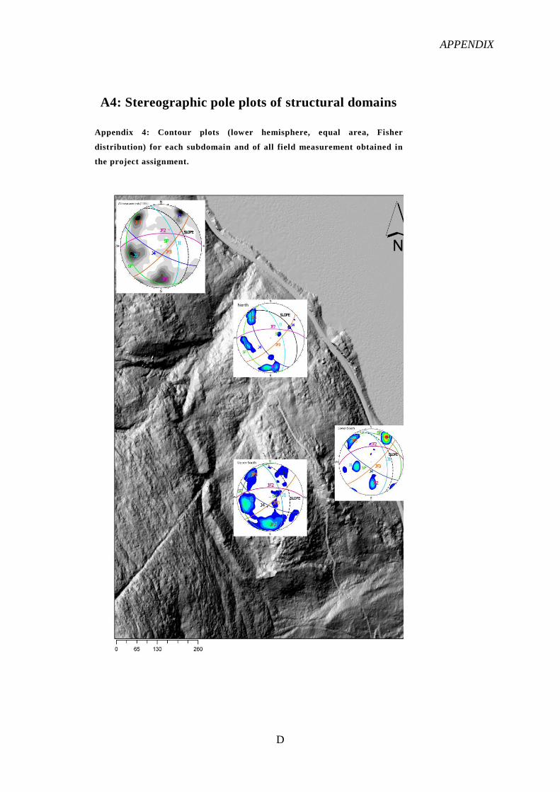
APPENDIX
D
A4: Stereographic pole plots of structural domains
Appendix 4: Contour plots (lower hemisphere, equal area, Fisher
distribution) for each subdomain and of all field measurement obtained in
the project assignment.

APPENDIX
E
A5: Normal stress calculation to potential failure surface
, MPa
, MPa
, , ,
Appendix 5: Subsection of Phase2 model for estimation of overburden down to an assumed potential
failure surface (green line). The overburden is used to determine the normal stress dependent material
shear strength parameters cohesion and friction angle as instantaneous values in RocLac (Rocscience,
2011).

APPENDIX
F
A6: Rock mass strength conversion in RocLab
Appendix 6: Output in RockLab. Instantaneous Samples for normal stress at
1,4MPa assumed.

APPENDIX
G
A7: Calculation of joint stiffness
Formulas for the calculations can be found in (Rocscience (2014b))
kn = normal shear stiffness
ks = shear stiffness
Ei = deformability modulus intact rock
Em = deformability modulus intact rock
L = mean joint spacing
Gm = rock mass shear modulus
Gi = intact rock shear modulus
Appendix 7a: Input values and results of joint set stiffness calculations
Rock parametes Symbol Value Source
Deformation modulus, intact rock Ei [MPa] 44300 Laboratory estimate obtained in project assignment
Deformation modulus, rock mass Em [MPa] 23036 RocLab (Rocscience, 2011)conversion, assumed Generalized H-B failure criterion
Poisson ratio Poissons 0,17 Laboratory estimat
Shear moduls, intact rock Gi [MPa] 18771 Formulas given in Myrvang (2001)
Shear modulus, rock mass Gm [MPa] 9761 Formulas given in Myrvang (2001)
Parameter Symbol Joint set values Source
J1 JF2 JF3 J4 SF
Joint set character
Average spacing L [m] 1 5 1 0,3 0,1 Field estimate
Joint stiffness Normal stiffness Kn [MPa/m] 47992 9598 47992 159972 479917 Formulas given in
Rocscience (2014a)
Shear stiffness Ks [MPa/m] 20335 4067 20335 67785 203355 Formulas given in
(Rocscience, 2014a)

APPENDIX
B
Appendix 7b:Epirical joint stiffness data given in (Sandøy, 2012)

APPENDIX
C
A8: Phase2 contour plots
Appendix 8.1: Analysis 2.12b (Model 2): 30%
reduced friction angle 50% reduced cohesion for
anisotropic hydrological conditions.(Initial values
given in Chapter 6). Location of the groundwater
table is highly uncertain.

APPENDIX
D
Appendix 8.2
Shear strain plot Model 1
Analysis 1.1: Initial rock mass
CSRF:1.9
Appendix 9a: Maximum shear strain plot Model 1
Appendix 8.3:
Shear strain plot Model 2: J1
Analysis 2.1: Initial rock mass
CSRF: 1.9

APPENDIX
E
Appendix 8.4:
Shear strain plot Model 3: J1 and SF
Analysis 2.1: Initial rock mass
CSRF: 1.8
Appendix 8.5:
Shear strain plot Model 4: All discontinuities
Analysis 4.4: Initial rock mass
CSRF: 1.1

APPENDIX
F
A9: Geometry for volume calculations
Appendix 9.1
Appendix 9.1a
Appendix 9.1b

APPENDIX
G
Appendix 9.2
Appendix 9.3
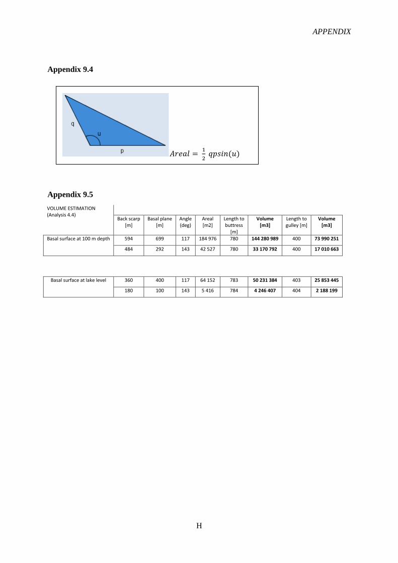
APPENDIX
H
Appendix 9.4
Appendix 9.5
VOLUME ESTIMATION (Analysis 4.4)
Back scarp [m]
Basal plane [m]
Angle (deg)
Areal [m2]
Length to buttress
[m]
Volume [m3]
Length to gulley [m]
Volume [m3]
Basal surface at 100 m depth 594 699 117 184 976 780 144 280 989 400 73 990 251
484 292 143 42 527 780 33 170 792 400 17 010 663
Basal surface at lake level 360 400 117 64 152 783 50 231 384 403 25 853 445
180 100 143 5 416 784 4 246 407 404 2 188 199