The History of the Cross Section of Returns
29
The History of the Cross Section of Returns September 2017 Juhani Linnainmaa, USC and NBER Michael R. Roberts, Wharton and NBER
Transcript of The History of the Cross Section of Returns

The History of the Cross Section of ReturnsSeptember 2017
Juhani Linnainmaa, USC and NBER
Michael R. Roberts, Wharton and NBER

Introduction
• Lots of anomalies
• 314 “factors” Harvey, Liu, and Zhu (2015)
• What is mechanism behind anomalies
• Unmodeled risk? Mispricing? Data-snooping?
• Empirical strategy
• Exploit comprehensive accounting data from 1926 to 2016
1. Pre-sample period (Jaffe et al ’89, Davis et al ‘00)
2. In-sample period
3. Post-sample period (Jagadeesh and Titman ’01, Schwert ’03,
McLean and Pontiff ‘16)
© Michael R Roberts 2

Key Findings
• 78% of anomalies “disappear” in pre- and post-periods
• Sharpe ratios, alphas, and information ratios all decrease; volatility and
covariation increase
• Including investment and profitability
• Sharpe ratio of 5-factor strategy ≈ Market Sharpe ratio (0.5) in pre-
• Choice of in-sample period critical to significance
• Small changes attenuate/eliminate many existing results
• 22% of anomalies survive
• Pre-sample: real investment, equity financing, distress, ROE/ROA
• Post-sample: Sales and earnings, total financing, distress, ROE/ROA
© Michael R Roberts 3
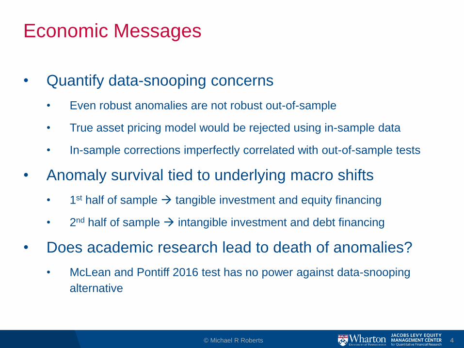
Economic Messages
• Quantify data-snooping concerns
• Even robust anomalies are not robust out-of-sample
• True asset pricing model would be rejected using in-sample data
• In-sample corrections imperfectly correlated with out-of-sample tests
• Anomaly survival tied to underlying macro shifts
• 1st half of sample tangible investment and equity financing
• 2nd half of sample intangible investment and debt financing
• Does academic research lead to death of anomalies?
• McLean and Pontiff 2016 test has no power against data-snooping
alternative
© Michael R Roberts 4
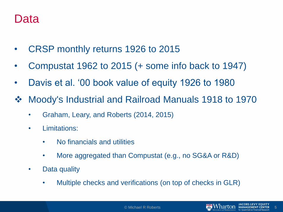
Data
• CRSP monthly returns 1926 to 2015
• Compustat 1962 to 2015 (+ some info back to 1947)
• Davis et al. ‘00 book value of equity 1926 to 1980
Moody's Industrial and Railroad Manuals 1918 to 1970
• Graham, Leary, and Roberts (2014, 2015)
• Limitations:
• No financials and utilities
• More aggregated than Compustat (e.g., no SG&A or R&D)
• Data quality
• Multiple checks and verifications (on top of checks in GLR)
© Michael R Roberts 5

Coverage
© Michael R Roberts 6
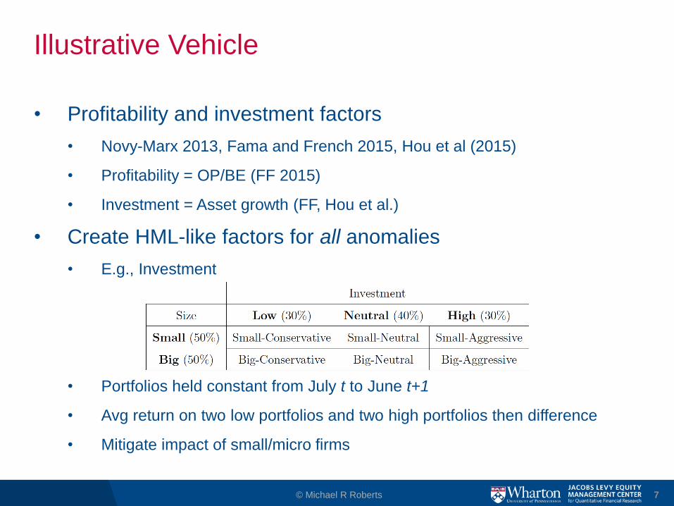
Illustrative Vehicle
• Profitability and investment factors
• Novy-Marx 2013, Fama and French 2015, Hou et al (2015)
• Profitability = OP/BE (FF 2015)
• Investment = Asset growth (FF, Hou et al.)
• Create HML-like factors for all anomalies
• E.g., Investment
• Portfolios held constant from July t to June t+1
• Avg return on two low portfolios and two high portfolios then difference
• Mitigate impact of small/micro firms
© Michael R Roberts 7
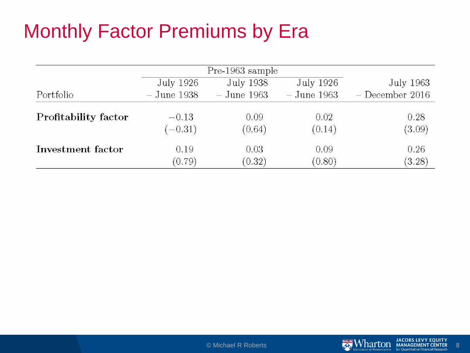
Monthly Factor Premiums by Era
© Michael R Roberts 8
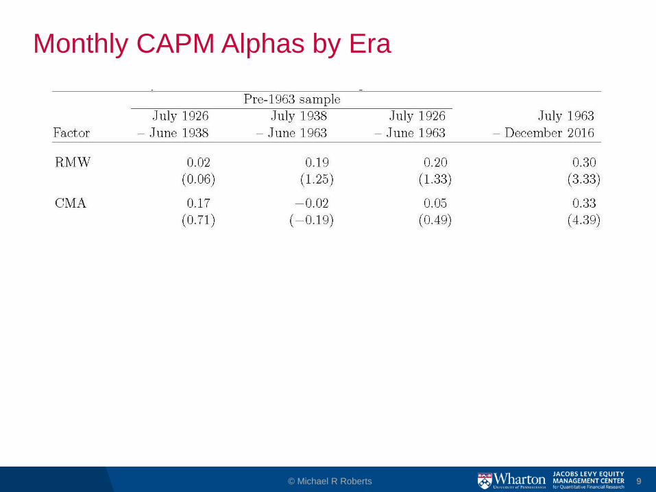
Monthly CAPM Alphas by Era
© Michael R Roberts 9
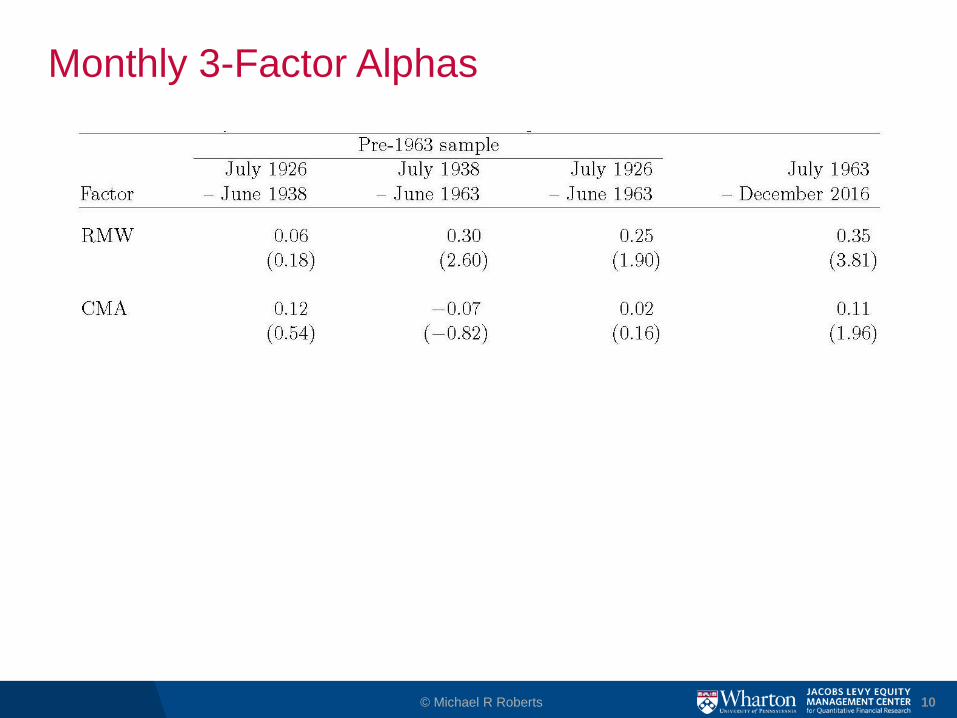
Monthly 3-Factor Alphas
© Michael R Roberts 10
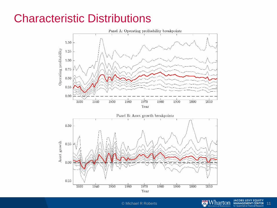
Characteristic Distributions
© Michael R Roberts 11

The Rest of the Zoo
© Michael R Roberts 12
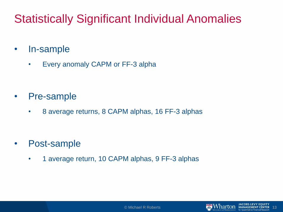
Statistically Significant Individual Anomalies
• In-sample
• Every anomaly CAPM or FF-3 alpha
• Pre-sample
• 8 average returns, 8 CAPM alphas, 16 FF-3 alphas
• Post-sample
• 1 average return, 10 CAPM alphas, 9 FF-3 alphas
© Michael R Roberts 13
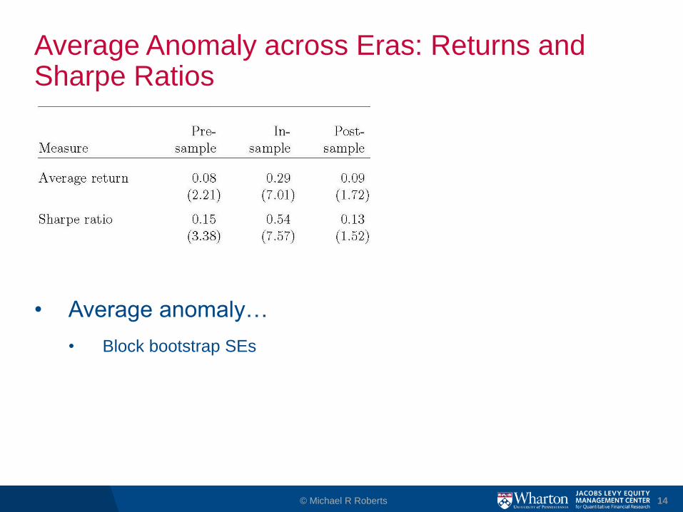
Average Anomaly across Eras: Returns and Sharpe Ratios
© Michael R Roberts 14
• Average anomaly…
• Block bootstrap SEs
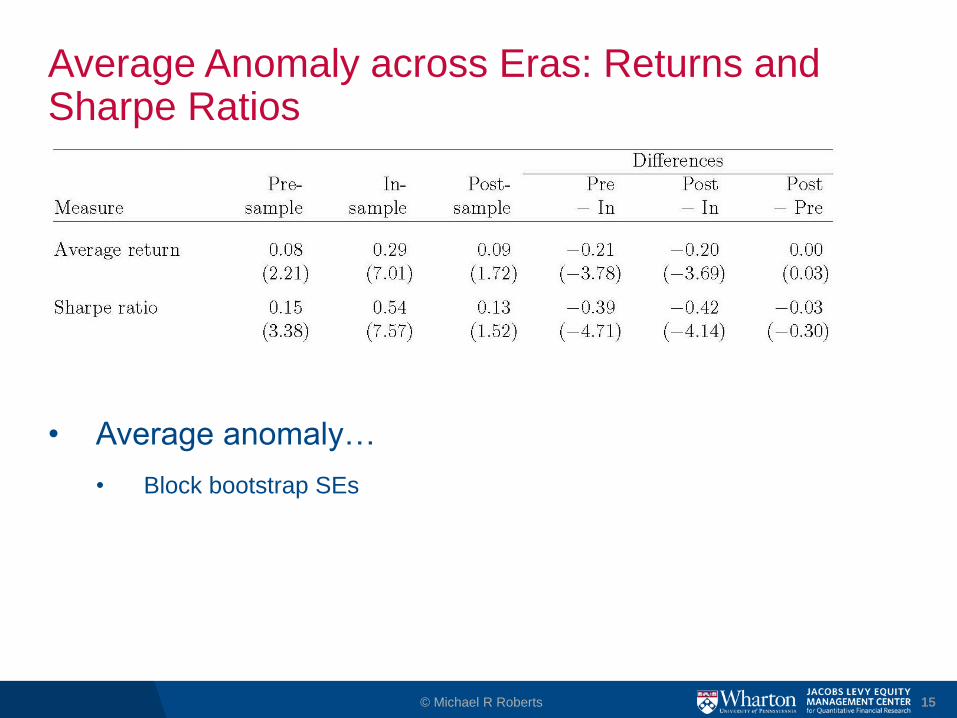
Average Anomaly across Eras: Returns and Sharpe Ratios
© Michael R Roberts 15
• Average anomaly…
• Block bootstrap SEs
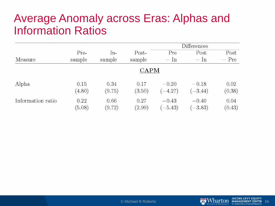
Average Anomaly across Eras: Alphas and Information Ratios
© Michael R Roberts 16

Average Anomaly across Eras: Alphas and Information Ratios
© Michael R Roberts 17
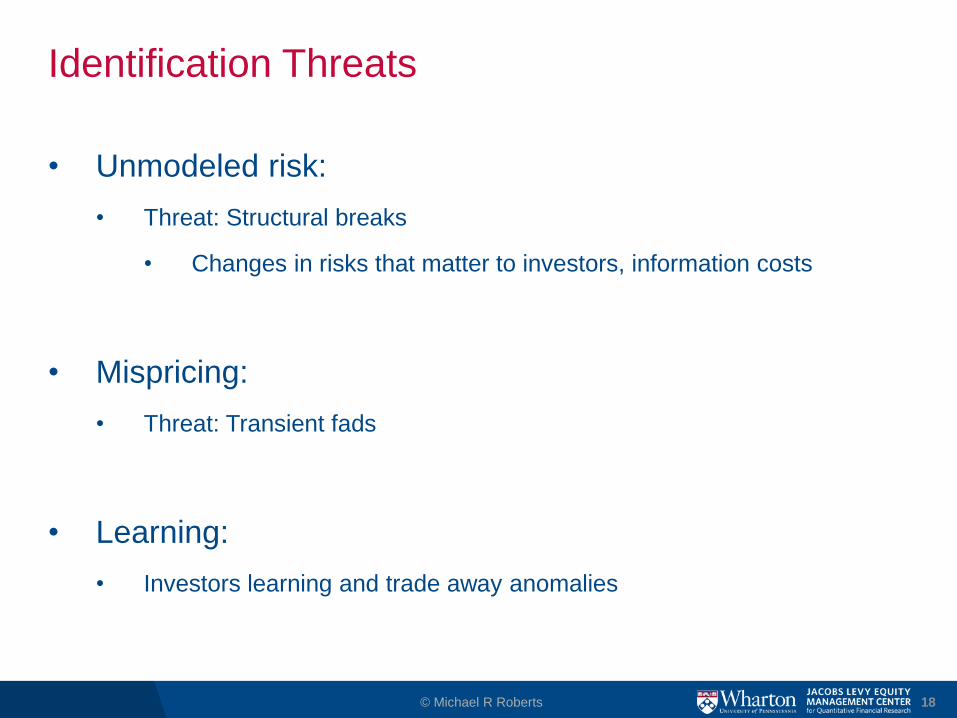
Identification Threats
• Unmodeled risk:
• Threat: Structural breaks
• Changes in risks that matter to investors, information costs
• Mispricing:
• Threat: Transient fads
• Learning:
• Investors learning and trade away anomalies
© Michael R Roberts 18

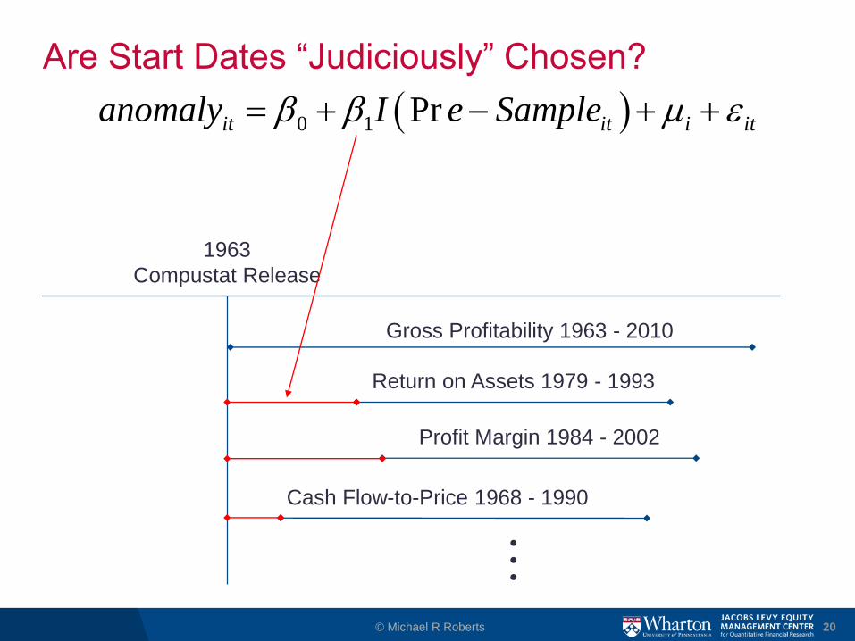
Are Start Dates “Judiciously” Chosen?
© Michael R Roberts 19
1963
Compustat Release
Gross Profitability 1963 - 2010
Return on Assets 1979 - 1993
Profit Margin 1984 - 2002
Cash Flow-to-Price 1968 - 1990
●
●
●
• All anomalies could have been measured as of 1963
• Was there a structural break around this time?
Are Start Dates “Judiciously” Chosen?
© Michael R Roberts 20
1963
Compustat Release
Gross Profitability 1963 - 2010
Return on Assets 1979 - 1993
Profit Margin 1984 - 2002
Cash Flow-to-Price 1968 - 1990
●
●
●
0 1 Prit it i itanomaly I e Sample
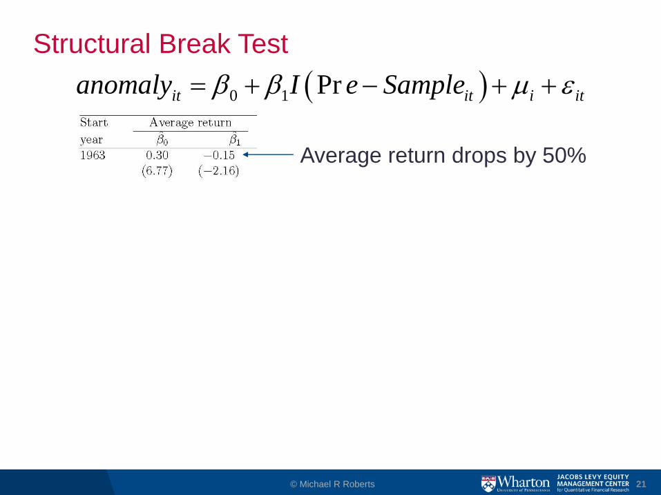
Structural Break Test
© Michael R Roberts 21
0 1 Prit it i itanomaly I e Sample
Average return drops by 50%

Structural Break Test
© Michael R Roberts 22
0 1 Prit it i itanomaly I e Sample
.
.
.Average return decline 40%-
80%
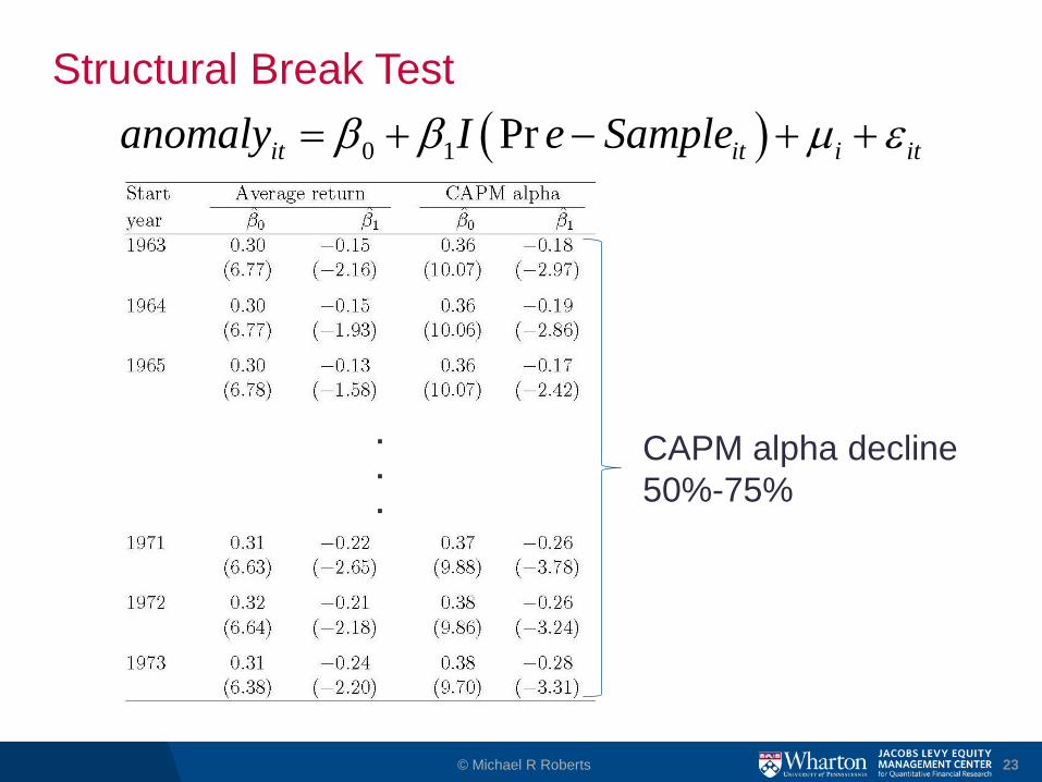
Structural Break Test
© Michael R Roberts 23
0 1 Prit it i itanomaly I e Sample
.
.
.
CAPM alpha decline
50%-75%

Structural Break Test
© Michael R Roberts 24
0 1 Prit it i itanomaly I e Sample
.
.
.
FF-3 alpha
decline
30%-90%

Correlation Structure of Returns
• How does an anomaly correlate with other anomalies
across eras?
• Motivated by Mclean and Pontiff (2016)
© Michael R Roberts 25
anomalyi,t
= a + b1Post
i,t+ b
2InSample Index
- i,t+ b
3PostSample Index
- i,t
+b4Post
i,t´ InSample Index
- i,t+ b
5Post
i,t´ PostSample Index
- i,t+ e
i,t
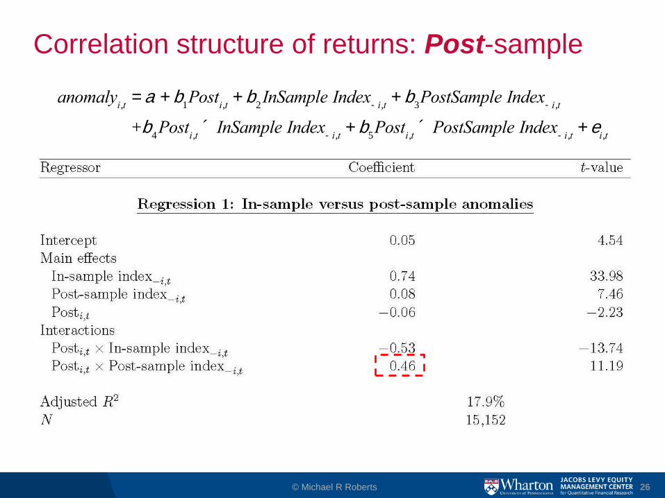
Correlation structure of returns: Post-sample
© Michael R Roberts 26
anomalyi,t
= a + b1Post
i,t+ b
2InSample Index
- i,t+ b
3PostSample Index
- i,t
+b4Post
i,t´ InSample Index
- i,t+ b
5Post
i,t´ PostSample Index
- i,t+ e
i,t

Correlation structure of returns: Pre-sample
© Michael R Roberts 27
anomalyi,t
= a + b1Pr e
i,t+ b
2InSample Index
- i,t+ b
3Pr eSample Index
- i,t
+b4Pr e
i,t´ InSample Index
- i,t+ b
5Pr e
i,t´ Pr eSample Index
- i,t+ e
i,t

Do In-sample Adjustments Work?
• Not really…
• Pr(Type I
error) = 30%
• Pr(Type II
error) = 26%
© Michael R Roberts 28

Conclusions and Future Work
• Half-empty
• Data-snooping is severe
• Statistical adjustments have limitations
Out-of-sample testing (new data, holdout samples)
• Half-full
• Persistent violations of common AP models
• Appear correlated with economic fundamentals
• In-progress:
• What is the “right” model?
• How does this model tie into economic fundamentals?
© Michael R Roberts 29