Richard HornbeckHarvard University and NBER

Pinar KeskinWellesley College

The Historically Evolving Impact of the Ogallala Aquifer:Agricultural Adaptation to Groundwater and Drought

September 2012Discussion Paper 12-39

heep@harvard.edu

www.hks.harvard.edu/m-rcbg/heep

Harvard Environmental Economics ProgramD E V E L O P I N G I N N O VAT I V E A N S W E R S T O T O D AY ’ S C O M P L E X E N V I R O N M E N TA L C H A L L E N G E S

The Historically Evolving Impact of the Ogallala Aquifer:

Agricultural Adaptation to Groundwater and Drought

Richard Hornbeck

Harvard University and NBER

Pinar Keskin

Wellesley College

The Harvard Environmental Economics Program

The Harvard Environmental Economics Program (HEEP) develops innovative answers to today’s

complex environmental issues, by providing a venue to bring together faculty and graduate students

from across Harvard University engaged in research, teaching, and outreach in environmental and

natural resource economics and related public policy. The program sponsors research projects,

convenes workshops, and supports graduate education to further understanding of critical issues in

environmental, natural resource, and energy economics and policy around the world.

Acknowledgments

The Enel Endowment for Environmental Economics at Harvard University provides major support

for HEEP. The Endowment was established in February 2007 by a generous capital gift from Enel

SpA, a progressive Italian corporation involved in energy production worldwide. HEEP receives

additional support from the affiliated Enel Foundation.

HEEP is also funded by grants from the Alfred P. Sloan Foundation, the James M. and Cathleen D.

Stone Foundation, Chevron Services Company, Duke Energy Corporation, and Shell. HEEP enjoys

an institutional home in and support from the Mossavar-Rahmani Center for Business and

Government at the Harvard Kennedy School. HEEP collaborates closely with the Harvard

University Center for the Environment (HUCE). The Center has provided generous material

support, and a number of HUCE’s Environmental Fellows and Visiting Scholars have made

intellectual contributions to HEEP. HEEP and the closely-affiliated Harvard Project on Climate

Agreements are grateful for additional support from the Belfer Center for Science and International

Affairs at the Harvard Kennedy School, ClimateWorks Foundation, the Qatar National Food

Security Programme, and Christopher P. Kaneb (Harvard AB 1990).

Citation Information

Hornbeck, Richard, and Pinar Keskin. “The Historically Evolving Impact of the Ogallala Aquifer:

Agricultural Adaptation to Groundwater and Drought,” Discussion Paper 2012-39, Cambridge,

Mass.: Harvard Environmental Economics Program, September 2012.

The views expressed in the Harvard Environmental Economics Program Discussion Paper Series

are those of the author(s) and do not necessarily reflect those of the Harvard Kennedy School or of

Harvard University. Discussion Papers have not undergone formal review and approval. Such

papers are included in this series to elicit feedback and to encourage debate on important public

policy challenges. Copyright belongs to the author(s). Papers may be downloaded for personal use

only.

The Historically Evolving Impact of the Ogallala Aquifer:

Agricultural Adaptation to Groundwater and Drought∗

Richard Hornbeck

Harvard University and NBER

Pinar Keskin

Wellesley College

July 2012

Abstract

Agriculture on the American Great Plains has been constrained historically by

water scarcity. In the latter half of the 20th century, technological improvements en-

abled farmers over the Ogallala aquifer to extract groundwater for large-scale irrigation.

Comparing counties over the Ogallala with nearby similar counties, groundwater access

increased agricultural land values and initially reduced the impact of droughts. Over

time, land-use adjusted toward high-value water-intensive crops and drought-sensitivity

increased. Farmers in nearby water-scarce counties have adopted lower-value drought-

resistant practices that fully mitigate their naturally higher drought-sensitivity. The

historically evolving impact of the Ogallala aquifer illustrates the importance of wa-

ter for agricultural production, but also the large scope for agricultural adaptation to

groundwater and drought.

∗For many helpful comments and suggestions, we thank seminar participants at AEA, Bocconi, Brown,Columbia, EHA, Harvard, IIES, Kansas, Miami-OH, Michigan, Michigan State, NBER, NEUDC, PERC,Queen’s, RES, Santa Barbara, Toronto, Tufts, UPF, Vanderbilt, Wellesley, World Bank, and Yale. For finan-cial support, we thank the Harvard University Center for the Environment and the Harvard SustainabilityScience Program. Melissa Eccleston, James Feigenbaum, Jan Kozak, and Jamie Lee provided excellentresearch assistance.

Water resources are critical to agricultural development in many arid regions, such as the

Western United States (Coman 1911; Hansen, Libecap, and Lowe 2011) and India (Rao 1979;

Shah 1993; Moench 1996; FAO 1999; Schoengold and Zilberman 2007; Keskin 2009). Water

scarcity is often exacerbated by inefficient water allocation, and much research has focused on

common pool externalities and the institutional structure for water allocation (Gisser 1983;

Ostrom 1990; Provencher and Oscar 1993; Blomquist 1994; Aggarwal and Narayan 2004;

Foster and Rosenzweig 2008; Sekhri 2008; Rosegrant et al. 2009; Ostrom 2011; Libecap

2011). It is less known how agricultural land-use and drought sensitivity adapt to water

availability in the short-run and, of more interest, evolve over many decades.1 Historical

changes in groundwater access provide a unique opportunity to identify how agriculture

adapts to available water resources and the threat of drought.

This paper analyzes the impacts of groundwater on agricultural land-use and drought

sensitivity, exploiting local variation in Plains counties’ access to the Ogallala aquifer. The

Ogallala was formed by ancient runoff from the Rocky Mountains, trapped below the modern

Great Plains, and it maintains distinct irregular boundaries that cut across modern soil

groups and natural vegetation regions. The Ogallala was first discovered in the 1890s,

but it remained mainly inaccessible. Following World War II, improved pumps and center

pivot irrigation technology made Ogallala groundwater available for large-scale irrigated

agriculture.

The baseline empirical specifications compare counties over the Ogallala with nearby

counties in the same state and soil group, controlling for longitude, latitude, average precip-

itation, and average temperature. Historical county-level data are drawn from the Census

of Agriculture and merged with a United States Geological Survey map of the Ogallala’s

boundary. Extended empirical specifications estimate the interaction between groundwater

and drought, using annual data on crop yields and drought severity. Ogallala counties and

non-Ogallala counties had similar characteristics prior to improved groundwater availability,

lending support to the identification assumption that Ogallala counties would otherwise have

been similar to non-Ogallala counties.

Increased access to groundwater has theoretically distinct short-run and long-run impacts

when farmers are able to adjust production methods faster than crop choice. In the short-run,

farmers increase irrigation intensity and crop yields become less sensitive to drought. In the

long-run, farmers also shift land toward water-intensive crops and crop yields become more

sensitive to drought. The net impact of groundwater on drought sensitivity is theoretically

1In general, the economic impacts of environmental change depend on how economic agents adapt in thelong-run (Mendelsohn, Nordhaus, and Shaw 1994; Schlenker, Hanemann, and Fisher 2006; Deschenes andGreenstone 2007; Guiteras 2009; Schlenker and Roberts 2009; Dell, Jones, and Olken 2011; Olmstead andRhode 2011; Hornbeck 2012).

1

ambiguous, depending on relative adjustment along the intensive (short-run) and extensive

(long-run) margins.2 In each period, the net present value of access to groundwater is

capitalized in agricultural land values.

Following the introduction of improved pumps and center pivot irrigation technology,

irrigated farmland increased substantially in counties over the Ogallala, both in absolute

terms and relative to nearby similar counties. Farmers increased irrigation first along the

intensive margin, shifting non-irrigated farmland to irrigation, before somewhat expanding

total farmland.

In the production of crops, farmers’ initial response was to increase the irrigation intensity

of corn and wheat. Irrigated corn acreages and irrigated wheat acreages increased, while

total corn and wheat acreages were mostly unchanged. In later periods, farmers shifted land

toward the more water-intensive corn.

Consistent with the model, farmers’ short-run adjustments reduced the impact of drought

on water-intensive corn yields. In the long-run, additional changes in land allocation re-

established the impact of drought on corn yields. Conversely, farmers in nearby water-scarce

counties have maintained drought-resistant agricultural practices that fully mitigate their

naturally higher sensitivity to drought.

Groundwater access remains a valuable agricultural asset, however, improving crops’

drought-resistance in the short-run and enabling the production of higher value crops in

the long-run. Estimated land value premiums capitalized the Ogallala’s peak value at $26

billion in the 1970’s and, as extraction rates remained high and water levels declined, the

Ogallala’s estimated value fell to $9 billion in 2002. The impact on agricultural revenues has

been increasing over time, particularly as farmers adjusted toward high-value water-intensive

corn. In the modern period, declining land values and rising revenues are consistent with

expectations that many areas will lose their current access to Ogallala groundwater.

Overall, the historically evolving impact of the Ogallala aquifer illustrates both the im-

portance of water for agricultural production and the large scope for agricultural adaptation

to groundwater and drought. Increased access to groundwater generates agricultural gains

in the short-run and long-run, but has distinct short-run and long-run impacts on drought

sensitivity due to adaptation of agricultural practices to available water resources. The long-

run impacts of water availability are difficult to observe in modern settings, as short-run

data do not capture the potential for long-run agricultural adaptation. As aquifers become

increasingly accessible in parts of Africa, and become depleted in parts of South Asia and

2In the opposite case, when farmers lose access to groundwater, the short-run response is to decreaseirrigation intensity and yields become more sensitive to drought. In the long-run, farmers shift land fromwater-intensive crops and yields become less sensitive to drought.

2

elsewhere, it is important to understand both the short-run and long-run impacts of ground-

water availability. The particular impacts of groundwater access may vary with agricultural

policy and other context-specific factors; however, for settings in which long-run historical

perspective is unavailable, the Ogallala provides a stark example of agricultural adaptation

to water availability and drought.

I Background on the Ogallala Aquifer

The Ogallala aquifer is one of the world’s largest underground freshwater sources. It was

formed by ancient runoff from the Rocky Mountains, trapped amidst accumulated sand,

gravel, clay, and silt. The Ogallala is a closed aquifer, essentially a nonrenewable resource,

that receives less than an inch of annual recharge due to minimal rainfall, high evaporation,

and low infiltration of surface water (Zwingle 1993; Opie 1993; McGuire et al. 2003).3

The Ogallala underlies 174,000 square miles of the Great Plains from the Texas panhandle

to South Dakota. The Ogallala’s boundaries are sharply defined by the location of ancient

valleys and hills, which have long since been covered and obscured on the surface.4

The Ogallala was first discovered by the United States Geological Survey in the 1890s,

but was considered of limited agricultural importance (Webb 1931; US Department of Com-

merce 1937). Windmill pumps could only provide small quantities of water, approximately

enough to irrigate 5 acres or provide for 30 cattle (Cunfer 2005). In a 1928 bulletin, the Ne-

braska Agricultural Extension Service highlighted the need for improved irrigation methods

to supplement scarce rainfall and streams; while “the underground water supply is abun-

dant,” there are insufficient means of “lifting it to the surface and applying it to the land”

(Weakley and Zook 1928). Groundwater irrigation was thought to be of great potential

value, particularly in raising corn yields, but pumps were small and expensive (Weakly 1932;

Brackett and Lewis 1933; Weakly 1936).

After World War II, automobile engines were adapted to power improved pumps, lifting

groundwater cheaply and in larger volumes. In the 1950’s, Nebraska Agricultural Exten-

sion Service bulletins discuss the growing importance of groundwater irrigation pumps (Epp

1954). Thorfinnson and Epp (1953) report that pump irrigation increases corn yields and

“serves as partial insurance against the hazards of drought.” Rhoades et al. (1954) discuss

3Artificial recharge has been considered but is infeasible. The 1968 Texas Water Plan considered divertingwater from the Mississippi River, but the Army Corps of Engineers estimated an annual requirement of 50billion kilowatts of electricity ($5 billion in 2010) and Texas abandoned the plan (Opie 1993).

4Local irrigation potential from the Ogallala is determined by three main characteristics: (1) depth ofwater (distance between the ground surface and the surface of the aquifer); (2) saturated thickness (distancefrom surface of the aquifer to the Triassic clay bottom of the aquifer); (3) specific yield (amount of waterthat can be extracted from a unit volume of saturated ground). Most areas retain sufficient water for localvariation in these characteristics to have little first-order importance for current land-use; as water levelscontinue to decline, however, these characteristics will become increasingly important.

3

how, as lands become irrigated, farmers can adjust corn “production practices to take full

advantage of irrigation water.” To guide adaptation in sub-humid Plains areas, Gertel et

al. (1956) draw lessons from a local Nebraska river basin: through production adjustments,

irrigation allows a higher-value crop rotation, with an emphasis on corn, and provides partial

insurance against drought.

In these early years, groundwater was mainly pumped into open irrigation furrows. Sprin-

kler systems were not widely adopted due to technical limitations and high costs (Bonnen et

al. 1952).5 In Texas, agricultural bulletins in 1952 focused on wheat production, for which

irrigation “is generally a practice of supplementing the natural rainfall and is not an intensive

irrigation of the crop” (Porter et al. 1952). “Only a limited amount of corn is grown” and

“practically all of the corn acreage is under irrigation because of the low natural rainfall”

(Rogers and Collier 1952).

Groundwater irrigation increased substantially with the subsequent introduction and

adoption of center pivot technology. Originally invented in 1949 by a Colorado farmer,

Frank Zybach, the “self-propelled sprinkling apparatus” combined recent advances in tur-

bine pumps, steel and aluminum pipes, and lawn sprinklers.6 Center pivot technology was

particularly suited to the Great Plains: able to direct water to plants with minimal evap-

oration in dry windy weather and able to accommodate large fields with hilly or sandy

land.

Zybach’s patent was granted in 1952 and he moved home to Nebraska and partnered

with a local businessman to begin manufacturing prototypes. Early center pivot machines

were unreliable; in 1954, they sold the patent to the Nebraska-based Valley Manufacturing

Company, who improved the design and began large-scale production and distribution. Com-

petition increased after Zybach’s original patent expired in 1969, though Nebraska remains

the hub of the center pivot irrigation industry.

As pumping and center pivot irrigation technologies were improved and adopted, Ogal-

lala groundwater became increasingly used for irrigation and farmers’ withdrawals quickly

surpassed the aquifer’s natural recharge rate. The USGS estimates that groundwater with-

drawals quintupled from 1949 to 1974 and water tables have declined substantially from

5From Bonnen et al. (1952), “Use of Irrigation Water on the High Plains,” Texas Bulletin 756: “A fewoperators have attempted to overcome the disadvantage of steep slopes and extremely sandy soils throughthe use of sprinkler systems. These have the advantage of providing an even distribution of water on landdifficult to water by other means. The practice has not been widely adopted partly because of a greatlyincreased investment, higher pumping costs, the additional labor involved in moving the system over theland, the difficulty of applying water rapidly enough especially during periods of high temperatures, and theuneven wetting of the soil during periods of windy weather.”

6For first-hand accounts of the technology’s introduction and improvement, seehttp://www.livinghistoryfarm.org/

4

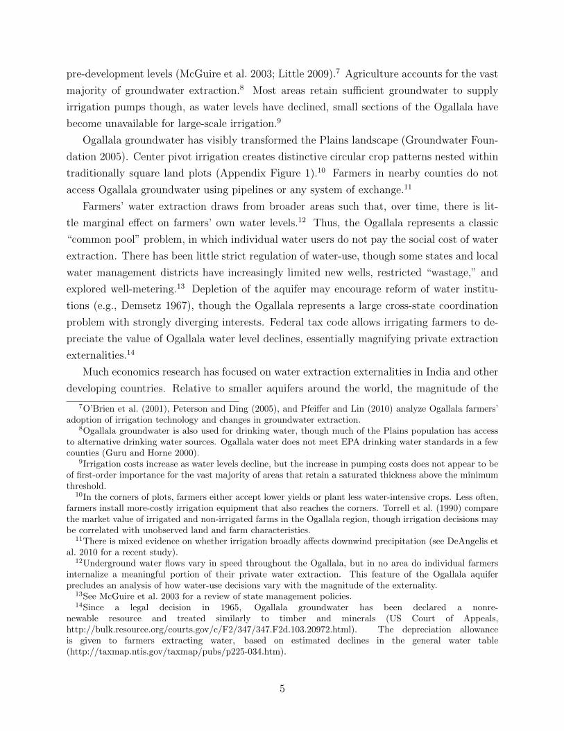
pre-development levels (McGuire et al. 2003; Little 2009).7 Agriculture accounts for the vast

majority of groundwater extraction.8 Most areas retain sufficient groundwater to supply

irrigation pumps though, as water levels have declined, small sections of the Ogallala have

become unavailable for large-scale irrigation.9

Ogallala groundwater has visibly transformed the Plains landscape (Groundwater Foun-

dation 2005). Center pivot irrigation creates distinctive circular crop patterns nested within

traditionally square land plots (Appendix Figure 1).10 Farmers in nearby counties do not

access Ogallala groundwater using pipelines or any system of exchange.11

Farmers’ water extraction draws from broader areas such that, over time, there is lit-

tle marginal effect on farmers’ own water levels.12 Thus, the Ogallala represents a classic

“common pool” problem, in which individual water users do not pay the social cost of water

extraction. There has been little strict regulation of water-use, though some states and local

water management districts have increasingly limited new wells, restricted “wastage,” and

explored well-metering.13 Depletion of the aquifer may encourage reform of water institu-

tions (e.g., Demsetz 1967), though the Ogallala represents a large cross-state coordination

problem with strongly diverging interests. Federal tax code allows irrigating farmers to de-

preciate the value of Ogallala water level declines, essentially magnifying private extraction

externalities.14

Much economics research has focused on water extraction externalities in India and other

developing countries. Relative to smaller aquifers around the world, the magnitude of the

7O’Brien et al. (2001), Peterson and Ding (2005), and Pfeiffer and Lin (2010) analyze Ogallala farmers’adoption of irrigation technology and changes in groundwater extraction.

8Ogallala groundwater is also used for drinking water, though much of the Plains population has accessto alternative drinking water sources. Ogallala water does not meet EPA drinking water standards in a fewcounties (Guru and Horne 2000).

9Irrigation costs increase as water levels decline, but the increase in pumping costs does not appear to beof first-order importance for the vast majority of areas that retain a saturated thickness above the minimumthreshold.

10In the corners of plots, farmers either accept lower yields or plant less water-intensive crops. Less often,farmers install more-costly irrigation equipment that also reaches the corners. Torrell et al. (1990) comparethe market value of irrigated and non-irrigated farms in the Ogallala region, though irrigation decisions maybe correlated with unobserved land and farm characteristics.

11There is mixed evidence on whether irrigation broadly affects downwind precipitation (see DeAngelis etal. 2010 for a recent study).

12Underground water flows vary in speed throughout the Ogallala, but in no area do individual farmersinternalize a meaningful portion of their private water extraction. This feature of the Ogallala aquiferprecludes an analysis of how water-use decisions vary with the magnitude of the externality.

13See McGuire et al. 2003 for a review of state management policies.14Since a legal decision in 1965, Ogallala groundwater has been declared a nonre-

newable resource and treated similarly to timber and minerals (US Court of Appeals,http://bulk.resource.org/courts.gov/c/F2/347/347.F2d.103.20972.html). The depreciation allowanceis given to farmers extracting water, based on estimated declines in the general water table(http://taxmap.ntis.gov/taxmap/pubs/p225-034.htm).

5

Ogallala and the speed of underground water flow imply that most local water extraction is

soon drawn from further sources. Standard plot sizes begin at 160 acres on the US Plains,

much larger than in India, so wells have less temporary effect on neighboring wells.15 Large

plot sizes also imply that fixed costs of digging a well are relatively less important than the

marginal costs of water extraction.

Because farmers’ water extraction is almost entirely an externality, i.e., there is little local

variation in the degree of externality, this paper focuses on other questions concerning land-

use adaptation and drought sensitivity. For these questions, a relative advantage to studying

Ogallala groundwater is that the United States Geological Survey (USGS) has detailed maps

on the Ogallala’s location; thus, it is not necessary to infer groundwater availability from

constructed wells or other agricultural decisions. In addition, because the Ogallala is a

large closed aquifer, the annual availability of groundwater is less-affected by drought and

agricultural land-use. Over time, water levels are endogenous to agricultural activity, so the

empirical analysis assigns groundwater availability using USGS pre-development Ogallala

boundaries.

II Agricultural Adaptation to Groundwater and Drought

Technological innovations substantially increased water availability for agriculture over the

Ogallala. In this simple model, farmers can adjust the water-intensity of production on the

intensive margin (within crops) and the extensive margin (between crops). Depending on the

relative speed and magnitude of adjustment on the intensive and extensive margins, ground-

water access has different short-run and long-run impacts on the sensitivity of agricultural

production to drought. The overall productive value of groundwater is capitalized in land

values.

II.A Baseline Model of Agricultural Adaptation to Groundwater

Assume that a farmer uses water and land to produce rents from two crops, according to two

concave production functions, y1(w1, L1) and y2(w2, L2). Water and land increase production

of both crops, but the first crop is more water-intensive.16

The farmer maximizes total rents, subject to a water constraint (w1 + w2 = w) and a

land constraint (L1 + L2 = 1).17 The farmer’s optimal production decisions are functions of

15Plot sizes of 160 acres create a natural minimum 0.4 kilometer buffer between wells, which is often thepolicy goal in developing countries to reduce the immediate impact of farmers’ extraction on neighbors’ waterlevels. Over time, depending on terrain characteristics, aquifer water flows underground to equalize levels.

16In particular, we introduce three assumptions. First, the marginal product of water is higher for thefirst crop: ∂y1/∂w1 > ∂y2/∂w2 > 0. Second, the marginal product of water declines slower for the first crop:∂2y2/(∂w2)2 < ∂2y1/(∂w1)2 < 0. Third, water and land are complementary for both crops, but weakly moreso for the first crop: ∂2y1/∂L1∂w1 ≥ ∂2y2/∂L2∂w2 > 0.

17While water availability is not actually subject to a hard constraint, this simplified model captures the

6

the water endowment: w∗1(w), L∗

1(w), w∗2(w), L∗

2(w).

An increase in the water endowment, i.e., a technological improvement in access to Ogal-

lala groundwater, affects agricultural production along the intensive and extensive margins:

(1)∂w∗

1(w)

∂w> 0 and

∂L∗1(w)

∂w> 0.

On the intensive margin, the farmer uses more water for the water-intensive crop. On the

extensive margin, land is shifted toward the water-intensive crop.18 Refer to the Theory

Appendix for a proof of the comparative statics in equation (1).

In a dynamic setting, agricultural adjustment may be delayed on the intensive margin

and/or extensive margin.19 Agricultural land-use adjustment may be delayed by switching

costs, or otherwise constrained by agricultural policy. Agricultural rents increase as produc-

tion adjusts along both margins. Agricultural land values increase immediately in antici-

pation of later rent increases, to the extent that the increase in groundwater availability is

unexpected.

II.B Adaptation to Drought Risk and Groundwater

Of further interest is how a farmer adapts to the threat of drought, particularly when there

is a change in groundwater availability. Assume that a risk-neutral farmer’s agricultural

production function depends on an additional drought term: y1(w1, L1, d) + y2(w2, L2, d).

Drought d is unexpected, reflecting deviations from average weather conditions, and farmers

cannot respond by changing water or land inputs.20 Groundwater partially mitigates the

negative impact of drought, particularly for the water-intensive crop.21

The farmer continues to maximize total rents, subject to constraints on water and

land. Given optimal allocations of water and land, the impact of drought is given by:

∂y1(L∗1, w

∗1, d)/∂d + ∂y2(L

∗2, w

∗2, d)/∂d. Of particular interest, an increase in the water en-

intuition of cases where the costs of obtaining water for irrigation are lowered by improved technologicalaccess to Ogallala groundwater.

18Changes in water usage for the less water-intensive crop (∂w∗2(w)/∂w) can be positive or negative,

depending on the production function parameters.19The increase in groundwater availability may also be gradual, as pumping and center pivot irrigation

technologies improve.20In practice, a farmer may partially adjust inputs when a drought occurs; for the model, it is only

necessary that a farmer is less able to adjust inputs after a drought is known than before the season began.21In particular, we introduce two additional assumptions. First, drought decreases the productivity of

land for both crops, but drought has a larger negative effect on the water-intensive crop: ∂2y1/∂L1∂d <∂2y2/∂L2∂d < 0. Second, drought increases the productivity of water for both crops, but more so for thewater-intensive crop: ∂2y1/∂w1∂d > ∂2y2/∂w2∂d > 0.

7

dowment has an ambiguous effect on the impact of drought:

(2)d

dw̄

[∂y1∂d

+∂y2∂d

]=

(∂2y1∂d∂w1

∂w∗1

∂w̄+

∂2y2∂d∂w2

∂w∗2

∂w̄

)︸ ︷︷ ︸

>0

+

(∂2y1∂L1∂d

− ∂2y2∂L2∂d

)∂L∗

1

∂w̄︸ ︷︷ ︸<0

.

On the intensive margin, an increase in water mitigates the impact of drought on each crop

(the first term). On the extensive margin, however, land shifts toward the more drought-

sensitive crop (the second term). The water-intensive crop may also become more sensitive

to drought as the land allocation shifts (e.g., growing corn in the Texas panhandle).

If land allocations are constrained in the short-run, an increase in the water endowment

only increases water usage on the intensive margin and mitigates the impact of drought. In

the long-run, however, as land allocations adjust, drought has more impact and may even

reduce agricultural production more than before. The Theory Appendix provides a proof of

this general case.

For a stark example, consider a plausible special case in which a farmer maximizes

L1y1(w1, d) + L2y2(w2, d) subject to w1L1 + w2L2 = w̄ and L1 + L2 = 1. After an in-

crease in the water endowment, in the short-run, per-acre crop water usage increases and

the impact of drought is mitigated. In the long-run, however, the farmer shifts land to

the water-intensive crop (∂L∗1(w)/∂w > 0) and per-acre crop water usage is unchanged

(∂w∗1(w)/∂w = ∂w∗

2(w)/∂w = 0). Thus, in the long-run, an increase in the water endow-

ment magnifies the impact of drought. The Theory Appendix provides a proof of this special

case.

The comparative statics are intuitive for a symmetric loss of access to groundwater. In

the short-run, crop choice remains fixed and there is less available water, so drought has a

larger impact on production. In the long-run, crop choice shifts toward the drought-resistant

crop and the impact of drought is mitigated. If there is sufficient change in crop choice, then

the impact of drought may become even less than before the loss of groundwater. In the

cross-section, areas without groundwater may sufficiently adapt toward non-water-intensive

crops to fully mitigate their naturally higher impact of drought.

III Data Construction and County Differences by Ogallala Share

III.A Census Data and Spatial Patterns

Historical county-level data are available every five years from the US Census of Agriculture

(Gutmann 2005; Haines 2005).22 The main variables of interest include: irrigated acres

and total acres of agricultural land, harvested acres and bushels of corn and wheat, value

22We thank Haines and collaborators for providing additional data.

8

of agricultural revenue, and value of agricultural land. The empirical analysis focuses on a

balanced panel of 368 Plains counties, from 1920 to 2002, for which data are available in

every period of analysis. To account for occasional changes in county borders, census data

are adjusted in later periods to maintain 1920 county definitions (Hornbeck 2010).

Figure 1 maps the Ogallala aquifer, overlaid with county borders in 1920. The shaded

area represents the USGS’s estimated original boundary of the aquifer, prior to intensive

use for agriculture. The sample is restricted to counties within 100 kilometers of the aquifer

boundary.

Figure 2 maps the 368 sample counties, shaded to reflect the irrigated percent of county

land in 1935 (panel A) and 1974 (panel B). In 1935, there was little irrigation in all sample

counties, aside from a few counties on major rivers. By 1974, irrigation increased substan-

tially in counties over the Ogallala, while counties within 100km were relatively unchanged.

Spatial patterns in agricultural land values are consistent with large economic impacts of

groundwater access. Figure 3 shows counties in 1920 (panel A) and 1964 (panel B), shaded in

each year to reflect their quintile in the distribution of counties’ average value of agricultural

land per county acre. There are strong regional determinants of land values; within local

areas, however, Ogallala counties and non-Ogallala counties had similar land values in 1920.

By 1964, land values are generally higher over the Ogallala than in nearby counties not over

the Ogallala.

The empirical research design exploits spatial variation in access to Ogallala groundwater,

comparing counties over the Ogallala with nearby similar counties. To focus on comparisons

among “nearby similar counties,” the empirical specifications control for average differences

by state, soil group, longitude, latitude, average precipitation, and average temperature.

States, mapped in Figure 1, capture differences in region, state agricultural extension ser-

vices, and other state-level policies.

Figure 4 displays major soil groups in the Plains, as defined by the Soil Conservation

Service in 1951. The 1951 SCS map was scanned, traced in GIS software, and merged to

1920 county borders to assign each county the fraction of its area in each soil group. These

soil groups proxy for detailed regional determinants of agricultural production. For example,

“Alluvial Soils” occur along major rivers and predict higher irrigation in 1935. Conversely,

“Sand and Silt” in North-Central Nebraska is unproductive for agriculture. The Ogallala

boundary cuts across major soil groups; importantly, as the analysis effectively compares

Ogallala and non-Ogallala counties within the same soil group.

Climate and geographic location may also influence agricultural production, even within-

state and within-soil group. County-level data on average precipitation and temperature

are taken from PRISM data (PRISM 2004). County longitude and latitude are measured

9

using the coordinates of 1920 county centroids (NHGIS).23 Because non-Ogallala counties

surround the Ogallala region, there is variation in Ogallala access within similar climate,

longitude, and latitude.

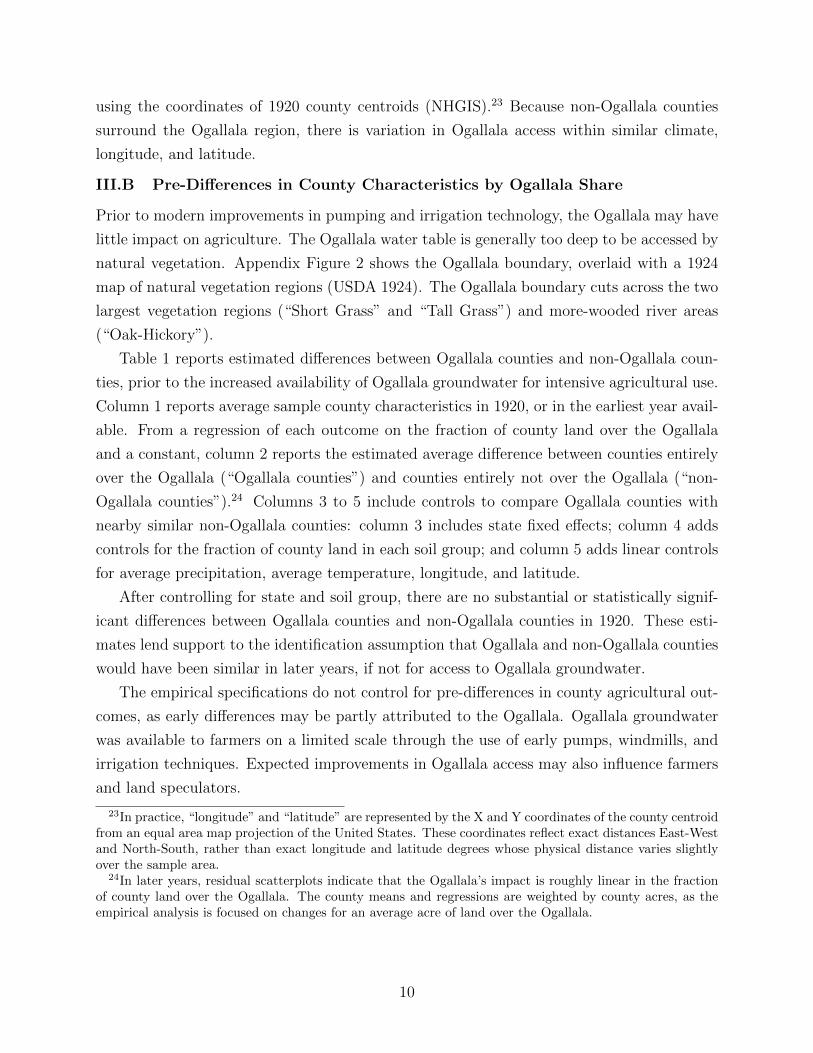
III.B Pre-Differences in County Characteristics by Ogallala Share

Prior to modern improvements in pumping and irrigation technology, the Ogallala may have

little impact on agriculture. The Ogallala water table is generally too deep to be accessed by

natural vegetation. Appendix Figure 2 shows the Ogallala boundary, overlaid with a 1924

map of natural vegetation regions (USDA 1924). The Ogallala boundary cuts across the two

largest vegetation regions (“Short Grass” and “Tall Grass”) and more-wooded river areas

(“Oak-Hickory”).

Table 1 reports estimated differences between Ogallala counties and non-Ogallala coun-

ties, prior to the increased availability of Ogallala groundwater for intensive agricultural use.

Column 1 reports average sample county characteristics in 1920, or in the earliest year avail-

able. From a regression of each outcome on the fraction of county land over the Ogallala

and a constant, column 2 reports the estimated average difference between counties entirely

over the Ogallala (“Ogallala counties”) and counties entirely not over the Ogallala (“non-

Ogallala counties”).24 Columns 3 to 5 include controls to compare Ogallala counties with

nearby similar non-Ogallala counties: column 3 includes state fixed effects; column 4 adds

controls for the fraction of county land in each soil group; and column 5 adds linear controls

for average precipitation, average temperature, longitude, and latitude.

After controlling for state and soil group, there are no substantial or statistically signif-

icant differences between Ogallala counties and non-Ogallala counties in 1920. These esti-

mates lend support to the identification assumption that Ogallala and non-Ogallala counties

would have been similar in later years, if not for access to Ogallala groundwater.

The empirical specifications do not control for pre-differences in county agricultural out-

comes, as early differences may be partly attributed to the Ogallala. Ogallala groundwater

was available to farmers on a limited scale through the use of early pumps, windmills, and

irrigation techniques. Expected improvements in Ogallala access may also influence farmers

and land speculators.

23In practice, “longitude” and “latitude” are represented by the X and Y coordinates of the county centroidfrom an equal area map projection of the United States. These coordinates reflect exact distances East-Westand North-South, rather than exact longitude and latitude degrees whose physical distance varies slightlyover the sample area.

24In later years, residual scatterplots indicate that the Ogallala’s impact is roughly linear in the fractionof county land over the Ogallala. The county means and regressions are weighted by county acres, as theempirical analysis is focused on changes for an average acre of land over the Ogallala.

10

III.C Changes in County Characteristics by Ogallala Group

For a preliminary view of the data, Figure 5 plots average outcomes over time for two groups

of sample counties: counties less than 10% over the Ogallala, and counties more than 90%

over the Ogallala.25 By contrast, the main empirical specifications use continuous variation

in counties’ Ogallala share and control for other differences among sample counties.

Counties in both groups had similar low levels of irrigated farmland in 1935 (Panel

A). As pumping and irrigation technology improved, counties over the Ogallala increased

irrigation through the 1970’s. Irrigated corn acreage increased somewhat in Ogallala counties

from 1954 to 1964, and was substantially higher by 1978 (Panel B). In contrast, total corn

acreage changed similarly from 1920 through 1964, and only became substantially higher

in Ogallala counties by 1978 (Panel C).26 The value of farmland was relatively lower or

similar in Ogallala counties from 1920 through the 1940’s; after 1950, land values became

consistently higher in Ogallala counties than in non-Ogallala counties (Panel D).

IV Empirical Framework

In the main empirical specifications, outcome Y in county c is regressed on the fraction

of county area over the Ogallala, state fixed effects αs, the fraction of county area in each

soil group γg, and linear functions of four fixed county characteristics Xc (average rainfall,

average temperature, longitude, and latitude).27 These cross-sectional specifications are

pooled across all time periods, with each coefficient allowed to vary in each time period:

(3) Yct = βtOgallalaSharec + αst + γgt + θtXc + εct

In each time period, the estimated β reports the average difference between counties entirely

over the Ogallala and counties never over the Ogallala.28

The estimated β’s can be interpreted as the impact of the Ogallala in each year, under

the identification assumption that sample counties would have had the same average out-

comes in each year if not for the Ogallala. In practice, this identification assumption must

hold after controlling for other differences correlated with state, soil group, precipitation,

25Average outcomes for the in-between counties are between the averages for the two groups shown, butthis third category is omitted from the figure for increased clarity.

26Harvested corn acreages fell substantially during the 1930’s drought and widespread crop failure.27Parts of the sample region were severely eroded during the 1930’s Dust Bowl (Hornbeck 2012). The

empirical results are robust to controlling for erosion severity; in principle, however, counties’ land-use anderosion may be affected by counties’ Ogallala share. Thus, these controls are not included in the mainspecifications.

28Some counties are partly over the Ogallala, and this specification assumes that the effect of the Ogallalais linear in the fraction of county area over the Ogallala. From graphing county residual changes in irrigatedfarmland against county residual Ogallala shares, the effect of the Ogallala appears roughly linear in theshare of county area over the Ogallala.

11

temperature, longitude, and latitude. In this way, the research design exploits the sharp

spatial discontinuity created by the Ogallala’s irregular boundary. Robustness checks limit

the sample to counties that intersect the Ogallala boundary.

The Ogallala’s impact may vary over the analyzed region. For example, the Ogallala may

have less impact in areas with unproductive soil and more impact in areas with productive

soil and water deficiencies.29 For simplicity, the analysis reports the impact of the Ogallala

on the average acre of land over the Ogallala. For this purpose, the regressions are weighted

by county size.

Differences in the estimated β’s, from one year to another year, report the average change

for an Ogallala county relative to a non-Ogallala county over that time period. Differencing

the estimated coefficients is numerically equivalent to estimating equation (3) in differences

or with county fixed effects.30 The standard error of the difference is generally 20-40% lower

than the standard error of the two cross-sectional coefficients due to positive serial correlation

in county-level outcomes. The change in β’s can be interpreted as the changing impact of

the Ogallala, under the weaker identification assumption that sample counties would have

had the same average changes if not for the Ogallala.

For the statistical inference, standard errors are clustered at the county level to adjust

for heteroskedasticity and within-county correlation over time. When allowing for spatial

correlation among sample counties, the estimated standard errors increase by approximately

10-30%.31

V Results

V.A Irrigation and Farmland: Intensive vs. Extensive Margins

Table 2, column 1, reports the estimated impact of the Ogallala in each year on acres of

irrigated farmland per county acre. In 1935, irrigation was a statistically insignificant 0.4

percentage points lower in Ogallala counties than in non-Ogallala counties.32 By 1950, irri-

gation was a statistically insignificant 1.3 percentage points higher in Ogallala counties than

29Indeed, the preliminary figures indicate substantial variation along these lines in the impact the Ogallalaon irrigation and land values.

30Differencing and fixed effects are equivalent for two time periods; for this multi-period regression, thespecification is essentially separable for any two time periods. The explanatory variables are fully interactedwith time, such that the impact of each variable is allowed to vary in each year. The sample is also balancedin each regression, such that every county has data in every analyzed period. Thus, the estimated coefficientsin any one year are not influenced by county outcomes in any other year.

31Spatial correlation among counties is assumed to be declining linearly up to a distance cutoff and zeroafter that cutoff (Conley 1999). For a distance cutoff of 100 miles or 200 miles, the estimated Conleystandard errors are approximately 10-30% higher than the standard errors when clustering at the countylevel, depending on the outcome variable.

32Note that the first row of coefficients for each outcome are the same coefficients reported in column 5 ofTable 1.

12

in non-Ogallala counties. As groundwater irrigation technology improved and agricultural

production adjusted, this difference increased to 11.3 percentage points by 1978. Ogallala

counties maintained substantially higher irrigation levels through 1997.

Column 2 reports the estimated impact of the Ogallala on acres of total farmland per

county acre. The fraction of county land in farms was similar in Ogallala and non-Ogallala

counties through 1959, though higher in some periods. Since the 1960’s, the fraction of

county land in farms has been consistently higher by 5 to 7 percentage points in Ogallala

counties. This small relative increase mainly reflects a slower absolute decline in farmland

than in non-Ogallala counties.

Comparing the estimates in column 1 and column 2, initial adjustments in agricultural

production were mainly on the intensive margin. Farmers increased irrigation of existing

farmland, shifting land from dryland farming. Subsequently, farmers both increased irriga-

tion and relatively expanded production along the extensive margin of total farmland.

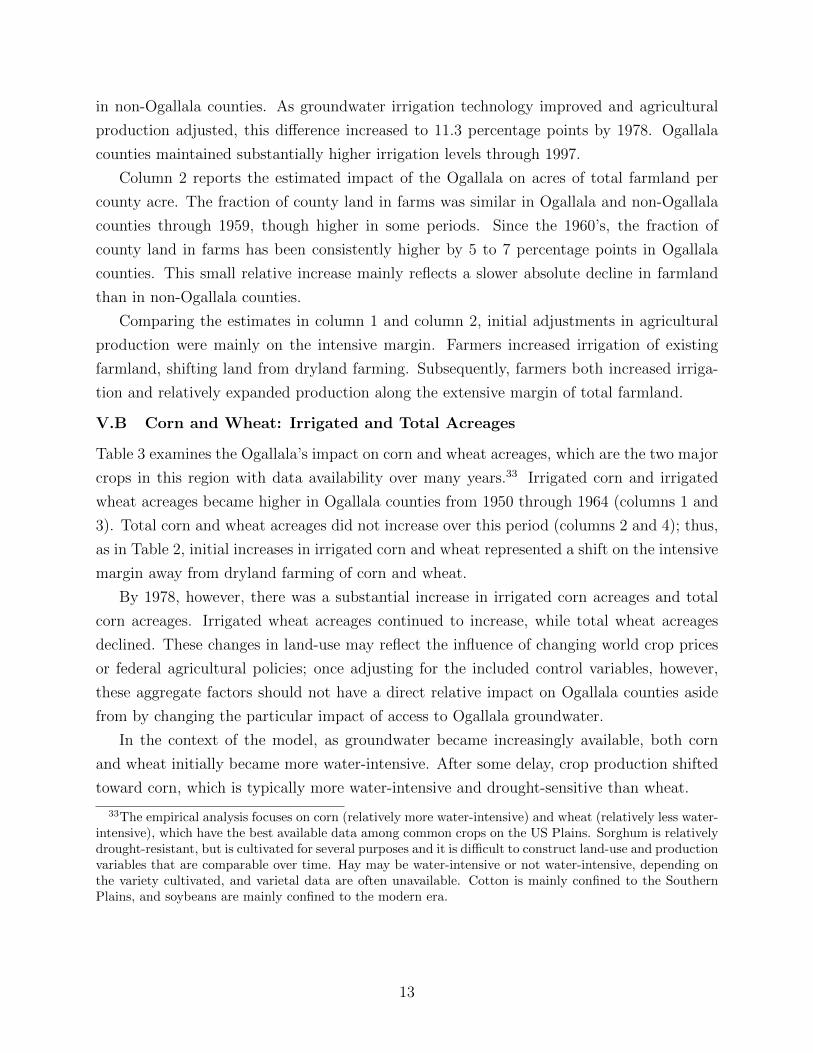
V.B Corn and Wheat: Irrigated and Total Acreages

Table 3 examines the Ogallala’s impact on corn and wheat acreages, which are the two major

crops in this region with data availability over many years.33 Irrigated corn and irrigated

wheat acreages became higher in Ogallala counties from 1950 through 1964 (columns 1 and

3). Total corn and wheat acreages did not increase over this period (columns 2 and 4); thus,

as in Table 2, initial increases in irrigated corn and wheat represented a shift on the intensive

margin away from dryland farming of corn and wheat.

By 1978, however, there was a substantial increase in irrigated corn acreages and total

corn acreages. Irrigated wheat acreages continued to increase, while total wheat acreages

declined. These changes in land-use may reflect the influence of changing world crop prices

or federal agricultural policies; once adjusting for the included control variables, however,

these aggregate factors should not have a direct relative impact on Ogallala counties aside

from by changing the particular impact of access to Ogallala groundwater.

In the context of the model, as groundwater became increasingly available, both corn

and wheat initially became more water-intensive. After some delay, crop production shifted

toward corn, which is typically more water-intensive and drought-sensitive than wheat.

33The empirical analysis focuses on corn (relatively more water-intensive) and wheat (relatively less water-intensive), which have the best available data among common crops on the US Plains. Sorghum is relativelydrought-resistant, but is cultivated for several purposes and it is difficult to construct land-use and productionvariables that are comparable over time. Hay may be water-intensive or not water-intensive, depending onthe variety cultivated, and varietal data are often unavailable. Cotton is mainly confined to the SouthernPlains, and soybeans are mainly confined to the modern era.

13

V.C Agricultural Land Values and Revenues

The model predicts that higher land values over the Ogallala capitalize the net present value

of agricultural rents from groundwater. In each period, land values reflect: (1) current

agricultural rents, (2) expected increases in rents from future improvements in pumping and

irrigation technology, (3) expected increases in rents from adjusting agricultural production,

and (4) expected decreases in rents from exhaustion of groundwater. Note that the impact

of Ogallala groundwater on land values depends not only on the quantity of technologically-

available water, but also technologies and prices that affect the value of water in agricultural

production.

In the 1950’s, after the introduction of improved pumping and irrigation technologies,

the value of agricultural land and buildings became consistently higher in counties over the

Ogallala (Table 4, column 1).34 The land value premium peaks at 51% in 1964 (0.415 log

points), and has since declined to 19% in 2002 (0.178 log points).

Column 2 reports the implied market valuation of Ogallala groundwater in each period,

based on the coefficients in column 1 and the total value of land over the Ogallala.35 Column 3

converts the estimated valuations into constant 2002 dollars using the Consumer Price Index:

the value of Ogallala groundwater rises from $8.9 billion in 1950 to a peak of $26 billion in

1974, and declines to $9.0 billion by 2002. Column 5 converts the estimated valuations into

constant 2002 dollars using a regional land value price index: the rise and fall in Ogallala

value is similar to column 3, though the Ogallala’s value peaks roughly 10 years earlier.36

Recent declines in land values over the Ogallala are consistent with expectations that

groundwater will become exhausted in some areas. An alternative interpretation is that

the marginal value of water has declined in recent periods (e.g., declining relative prices

of water-intensive crops). While agricultural rents are not directly observable, agricultural

revenues provide a useful proxy.37 Table 4, column 5, reports that agricultural revenues

have been higher over the Ogallala since the late 1940’s, but increased substantially in the

34Over this long time period, data are only available for the combined value of agricultural land andbuildings. From 1900 to 1940, when data are available separately for land and buildings, the value of landis the much larger component.

35The coefficient β implies that land values would decline by (eβ−1)eβ

percent, on average, in the absenceof Ogallala groundwater. This percent decline is multiplied by the total value of land over the Ogallala,estimated as the sum of each county’s total land value multiplied by its share of land over the Ogallala. Theestimates’ t-statistics are approximately the same as in column 1; they would be identical, but the estimatedlog point differences are converted to percent differences.

36The land value price index is defined as the 2002 value of land in sample counties with zero Ogallalashare, divided by that year’s value of land in sample counties with zero Ogallala share.

37If the agricultural production function were Cobb-Douglas, then percent differences in revenue equal thepercent differences in unobserved agricultural rents. However, Ogallala counties’ higher irrigation expensessuggest that factor shares may not be constant and higher revenues are likely to overstate the impact onrents.

14

1970’s as agriculture shifted toward greater corn acreages over the Ogallala. The impact on

revenues has increased in recent periods, as land values have declined, suggesting that the

marginal return to water remains high and decreased land values reflect market expectations

of exhaustion.38

The estimated Ogallala premiums in land values and revenues may reflect the combination

of a variety of factors, including: (1) increased allocation of land to high value crops, (2)

increased crop yields, (3) decreased irrigation costs, (4) general increases in yields of water-

intensive crops, and (5) general increases in prices of water-intensive crops. In particular,

the introduction of hybrid corn or increased corn prices may increase the Ogallala’s value

if the Ogallala enables counties to grow corn. The estimated marginal return to water

will inherently reflect the influence of prices and productivity of water-intensive activities.

For example, as policymakers consider the risk of an oil pipeline contaminating Ogallala

groundwater, these five factors jointly contribute to the policy-relevant valuation of Ogallala

groundwater for agricultural production.

Higher land values over the Ogallala do not appear to reflect increased demand for land

in the urban sector. In contrast to other areas of the United States, the sample region is

predominately rural and there is less impact of urban expansion on agricultural land values.

The Ogallala is not estimated to increase log county population or the fraction of population

living in urban areas (i.e., places with population greater than 2500). Further, the estimated

land value premiums are similar or higher when restricting the sample to 253 counties with

zero urban population in 1920 or 287 counties with less than 25% urban population in 1920.

V.D Robustness and General Equilibrium Spillovers

The empirical results appear robust to changes in the particular empirical specification, as

suggested by the unadjusted data reported in the maps (Figures 2 and 3) and aggregate

changes by Ogallala share (Figure 5). The results are generally insensitive to changing the

included control variables and/or their functional form. The results are also similar when

narrowing the main 368 county sample to 186 counties on the Ogallala boundary, i.e., with

Ogallala shares strictly between zero and one.

The estimated relative differences in Ogallala counties may not reflect the aggregate

impact of the Ogallala if there are spillover effects on non-Ogallala counties. There are

minimal direct spillovers in access to water, as Ogallala water is not directly transferred

to non-Ogallala counties for agricultural use. The Ogallala may also have limited indirect

38The estimated market valuation of the Ogallala may understate its potential value, to the extent thatgroundwater extraction externalities induce inefficient water-use. The estimates may overstate the value ofgroundwater, to the extent that groundwater access encourages greater fixed investments that are capitalizedin the value of agricultural land and buildings.

15

effects on agricultural prices because the Ogallala region represents a small share of national

and world agricultural production. However, to the extent that some markets are more

local, nearby non-Ogallala counties may be affected by changes in factor availability and

terms-of-trade.

To explore local spillover effects, a placebo test compares counties near the Ogallala to

counties further from the Ogallala. Restricting the sample to counties with zero Ogallala

share, equation (3) is modified to estimate the impact in each year of distance to the Ogallala

boundary. For ease of interpretation, distance is measured in units of 100km and made neg-

ative. The estimated coefficients are interpreted as the impact of the Ogallala on the nearest

sample counties, relative to the impact of the Ogallala on the furthest sample counties.

Table 5 reports estimates from this placebo test. For each of the main outcome vari-

ables, there is no substantial or statistically detectable relative impact of the Ogallala on

nearby non-Ogallala counties. When expanding the sample to counties 200km from the

Ogallala boundary for increased statistical power, there remains little detectable impact of

the Ogallala on nearby counties relative to further counties.

VI Groundwater and Drought: Short-run and Long-run Interaction Effects

The impact of groundwater on drought sensitivity depends on the relative speed and magni-

tude of land-use adjustment on the intensive and extensive margins. In response to increased

availability of Ogallala groundwater, farmers are estimated to have initially increased water-

use mainly on the intensive margin. Irrigated farmland, irrigated corn acreage, and irrigated

wheat acreage became higher in Ogallala counties; in contrast, there was little initial change

in total farmland, total corn acreage, and total wheat acreage. In later periods, farmers in-

creased total corn acreage, with some small increases in total farmland and small decreases

in wheat acreage.

Given these findings, the model predicts an initial decline in the sensitivity of corn yields

to drought. This effect is predicted to dissipate once total corn acreage increases, expanding

into arid drought-sensitive lands. An alternative interpretation is that non-Ogallala counties

have adapted to water scarcity by maintaining acreage in drought-resistant crops.

To explore the short-run and long-run impact of groundwater on drought sensitivity of

corn and wheat yields, annual county-level data are drawn from the National Agricultural

Statistics Service (NASS). In contrast to Census data on harvested acreages, the NASS

provides data on planted acreages of corn and wheat. Drought-damaged cropland is often

not harvested, so it is important to define crop yields as the log number of bushels produced

per planted acre. In the sample region, corn and wheat yields are only available in each year

16

for a limited number of counties between 1940 and 1993.39

Drought is defined according to the Palmer Drought Severity Index (PDSI), and annual

county-level PDSI data are drawn from the National Climatic Data Center (NCDC).40 The

PDSI uses cumulative rainfall and temperature to determine dryness or wetness, relative to

the local average climate. To focus on drought, the PDSI is set equal to zero in wet years

and the index ranges between zero and 7.22 with a 1.16 standard deviation. For ease of

interpreting the empirical estimates, we normalize this drought measure to have mean zero

and a standard deviation of one.

Focusing initially on non-Ogallala counties, from 1940 to 1993, background specifications

regress log crop yields on drought, with year fixed effects or state-by-year fixed effects.

Drought is estimated to have a large negative impact on corn yield and a moderate negative

impact on wheat yield. Irrigated crop yields are less-affected by drought than non-irrigated

crop yields, particularly for corn. These estimates are consistent with expectations that

corn is more water-intensive and drought-sensitive than wheat (Brower and Heibloem 1986;

Pimentel et al. 1997).

The main empirical specifications use variation in access to Ogallala groundwater, over

space and time, to estimate interaction terms between drought and the Ogallala. Based on

previous results, the 54 years of data are split into three 18-year eras: before widespread use

of Ogallala irrigation for corn and wheat (1940-1957), after increases in the water-intensity

of corn and wheat (1958-1975), and after a shift toward the more water-intensive corn (1976-

1993). Of particular interest is how the Ogallala affects the impact of drought in the second

and third eras, relative to the first era, conditional on a number of control variables.41

Formally, log crop yield Y in county c and year t is regressed on the triple interaction

between a county’s Ogallala share, normalized drought index, and a dummy for the second

era or third era (Ogallalac ×Droughtct × 1(e = 2) and Ogallalac ×Droughtct × 1(e = 3)).

The change in impact of Ogallala access on yield during average weather is captured by the

double interaction between a county’s Ogallala share and a dummy for the second era or

third era (Ogallalac×1(e = 2) and Ogallalac×1(e = 3)). As controls, the regression includes

county fixed effects (αc) and era-specific controls for state (γ1se), soil group (γ2ge), and linear

functions of average precipitation, average temperature, longitude, and latitude (γ3eXc). The

effect of drought is allowed to vary in each county by controlling for interactions between

39Before 1940, NASS data is available for few states and the 1930’s were otherwise atypical due to extremedrought, the Dust Bowl, and the Great Depression. After 1993, NASS data is available for fewer countieswithin these states.

40We thank Hansen, Libecap, and Lowe (2011) for providing PDSI data.41Drought mainly varies across years in the sample region, so it is not feasible to exploit only within-year

variation in drought intensity and access to Ogallala groundwater.

17

drought and county fixed effects (Droughtct×αc). The effect of drought is allowed to vary in

each era (Droughtct× 1(e = 2) and Droughtct× 1(e = 3)). In some specifications, the effect

of drought is also allowed to vary in each era and state (Droughtct × γ1se), each era and soil

group (Droughtct × γ2ge), or each era and linear functions of average precipitation, average

temperature, longitude, and latitude (Droughtct×γ3eXc). The full empirical specification is:

Yct = β1Ogallalac ×Droughtct × 1(e = 2) + β2Ogallalac ×Droughtct × 1(e = 3)(4)

+ β3Ogallalac × 1(e = 2) + β4Ogallalac × 1(e = 3)

+ αc + γ1se + γ2ge + γ3eXc

+ δ1Droughtct × αc + δ2Droughtct × 1(e = 2) + δ3Droughtct × 1(e = 3)

+ δ4Droughtct × γ1se + δ5Droughtct × γ2ge + δ6Droughtct × γ3eXc + εct

The main coefficients of interest are β1 and β2, which indicate how the Ogallala affects the

impact of drought in the second and third eras, relative to the first era. In addition, the

coefficients β3 and β4 indicate how the Ogallala affects yields during average weather in the

second and third eras, relative to the first era. The sample is balanced in each regression,

such that every county included has data in each period. There are fewer counties in each

sample, and the states with available data are reported along with the number of county

observations. The regressions continue to be weighted by county size, and standard errors

are clustered at the county level.

Table 6, panel A, reports estimates from equation (5) for corn yields. In the second era,

from 1958 to 1976, the Ogallala substantially mitigated the impact of drought on corn yields.

In years when drought was one standard deviation higher, Ogallala counties experienced a

34% to 45% productivity advantage over non-Ogallala counties (0.29 log points to 0.38 log

points), relative to average county-level differences in drought sensitivity. Because the sample

is restricted to 134 counties over 54 years in Nebraska, South Dakota, and Iowa, Column 1

imposes a restriction on the control variables that δ4 = δ5 = δ6 = 0, column 2 restricts only

δ6 = 0, and column 3 presents the full specification from equation (5). During this second

era, there was little change in corn yields during average weather conditions (-0.02 log points

to -0.05 log points).

In the third era, from 1977 to 1993, the Ogallala lost most of its effect on corn yields

during drought (-0.05 log points to 0.08 log points). Yields increased slightly during average

weather conditions from the second era to the third era (0.10 log points to 0.13 log points).

During this third era, as revenues increased substantially, the Ogallala’s main impact was

enabling expansion of high-value corn cultivation without inducing severe drops in yields

during average weather conditions or droughts. Similarly, by limiting corn cultivation, non-

18

Ogallala counties have maintained average yields and drought-resistance despite higher water

scarcity.

By comparison, panel B, reports estimates from equation (5) for wheat yields. The

Ogallala had little impact on wheat yields, which is more drought-resistant than corn.

VII Conclusion

Agriculture on the Plains has been constrained historically by water scarcity. In the lat-

ter half of the 20th century, technological improvements enabled farmers over the Ogallala

aquifer to extract groundwater for large-scale irrigation. Increased access to Ogallala ground-

water increased agricultural land values and initially reduced the impact of droughts. Over

time, land-use adjusted toward high-value water-intensive crops and drought-sensitivity in-

creased.

Lacking access to Ogallala groundwater, nearby counties have maintained lower-value

agricultural practices that are less water-intensive and more drought-resistant. While agri-

cultural land values and revenues remain lower in nearby counties, agricultural production

has adapted to water availability such that non-Ogallala counties are no more sensitive to

drought than heavily-irrigated Ogallala counties.

Scarce water resources have an important role in shaping agricultural production, par-

ticularly in arid drought-prone areas. In modern settings, however, it is difficult to observe

how agriculture adapts over time to available water resources and the threat of drought. As

aquifers become increasingly accessible in parts of Africa, and become depleted in parts of

South Asia and elsewhere, it is important to understand both the short-run and long-run

impacts of groundwater availability. The particular pattern of agricultural land-use adjust-

ment observed in this setting may reflect the influence of US agricultural policy and other

context-specific factors; however, for settings in which such historical perspective is unavail-

able, the historically evolving impact of the Ogallala aquifer provides a stark example of

the importance of water for agricultural production and also the large scope for long-run

agricultural adaptation to groundwater and drought.

19

20

REFERENCES Aggarwal, R.M. and T.A. Narayan. 2004. "Does inequality lead to greater efficiency in the use of local commons? The role of strategic investments in capacity," Journal of Environmental Economics and Management, 47, 163-182. Blomquist, W. 1994. “Changing Rules, Changing Games: Evidence from Groundwater Systems in Southern California,” in Rules, Games, and Common-Pool Resources, eds. Elinor Ostrom, Roy Gardner, and James Walker, Ann Arbor, MI: University of Michigan Press. Bonnen, C.A., W.C. McArthur, A.C. Magee, and W.F. Hughes. 1952. “Use of Irrigation Water on the High Plains.” Texas Agricultural Experiment Station, College Station, Texas Agricultural and Mechanical College System, Bulletin 756 (December). Brackett, E.E. and E.B. Lewis. 1933. “Pump Irrigation Investigations in Nebraska.” Agricultural Experiment Station, University of Nebraska College of Agriculture, Lincoln, Bulletin 282 (July). Brower, C., and Heibloem, M. 1986. "Irrigation water management: Irrigation water needs," Training Manual 3, Rome 7, FAO. Coman, K. 1911. "Some Unsettled Problems of Irrigation," American Economic Review, 1(1)1-19. Conley, T. 1999. “GMM estimation with cross sectional dependence.” J. of Econometrics, 92 (1)1-45. Cunfer, G., 2005. On the Great Plains: Agriculture and Environment. Texas A&M University Press, College Station. DeAngelis, A., F. Dominguez, Y. Fan, A. Robock, M. D. Kustu, and D. Robinson. 2010. "Evidence of enhanced precipitation due to irrigation over the Great Plains of the United States," Journal of Geophysical Research, 115. Dell, M., B. Jones, and B. Olken. 2011. “Temperature Shocks and Economic Growth: Evidence from the Last Half Century.” August, Mimeo. Demsetz, H. 1967. “Toward a Theory of Property Rights,” American Economic Review: Papers and Proceedings, 57, 347-359. Deschenes, O. and M. Greenstone. 2007. “The Economic Impacts of Climate Change: Evidence from Agricultural Output and Random Fluctuations in Weather.” American Economic Review, 97(1)354-385. Epp, A.W. 1954. “The Cost of Pumping Water for Irrigation in Nebraska.” Agricultural Experiment Station, University of Nebraska College of Agriculture, Lincoln, Bulletin 426 (November). FAO. 1999. Poverty Reduction and Irrigated Agriculture. International Programme for Technology and Research in Irrigation and Drainage. Food and Agricultural Organization of the United Nations, Rome.

21

Foster, A. and M. Rosenzweig, “Inequality and the Sustainability of Agricultural Productivity Growth: Groundwater and the Green Revolution in Rural India,” mimeo, 2008. Gertel, K., J.W. Thomas, T.S. Thorfinnson, and H.W. Ottoson. 1956. “Adjusting to Irrigation in the Loup River Area in Nebraska.” Agricultural Experiment Station, University of Nebraska College of Agriculture, Lincoln, Bulletin 434 (February). Gisser, M. 1983. "Groundwater: Focusing on the Real Issue," Journal of Political Economy, 91, 1001-1027. Groundwater Foundation. 2005. Rainmakers: A Photographic Story of Center Pivots. Lincoln, Nebraska. Guiteras, R. 2009. “The Impact of Climate Change on Indian Agriculture,” mimeo. Guru, M.V., and J.E. Horne. 2001. “The Ogallala Aquifer,” Water Resource Management, 48, 321-329. Gutmann, M.P. 2005. Great Plains Population and Environment Data: Agricultural Data. Ann Arbor: University of Michigan and ICPSR. Haines, M.R. 2005. Historical, Demographic, Economic, and Social Data: The United States, 1790–2000. Hamilton, NY: Colgate University and ICPSR. Hansen, Z., G. Libecap, and S. Lowe. 2011. "Climate Variability and Water Infrastructure: Historical Experience in the Western United States," in The Economics of Climate Change: Adaptations Past and Present, eds. Gary D. Libecap and Richard H. Steckel, May 2001, NBER, University of Chicago Press. Hornbeck, R. 2012. “The Enduring Impact of the American Dust Bowl: Short- and Long-run Adjustments to Environmental Catastrophe,” American Economic Review, Vol. 102, No. 4, pp. 1477-1507. Hornbeck, R. 2010. “Barbed Wire: Property Rights and Agricultural Development,” Quarterly Journal of Economics, 125, 767–810. Keskin, P. 2009. “Thirsty Factories, Hungry Farmers: Intersectoral Impacts of Industrial Water Demand,” mimeo, Kennedy School of Government. Libecap, G. 2011. "Institutional Path Dependence in Climate Adaptation: Coman's 'Some Unsettled Problems of Irrigation,'" American Economic Review Centenary Symposium, 101(1)64-80. Little, J. 2009. “The Ogallala Aquifer: Saving a Vital U.S. Water Source.” Scientific American, March. McGuire, V.L., Johnson, M.R., Schieffer, R.L., Stanton, J.S., Sebree, S.K., and Verstraeten, I.M., 2003, Water in storage and approaches to ground-water management, High Plains aquifer, 2000: U.S. Geological Survey Circular 1243. Mendelsohn, R., W. Nordhaus, and D. Shaw. 1994. "The impact of global warming on

22

agriculture: A Ricardian analysis," American Economic Review, 84(4)753-771. Moench, M. 1996. Groundwater policy: Issues and alternatives in India. Colombo: International Irrigation Management Institute. NHGIS, http://www.nhgis.org/, Minnesota Population Center, University of Minnesota. O’Brien, D.M., F.R. Lamm, L.R. Stone, and D.H. Rogers. 2001. “Corn-Yield and Profitability for Low- Capacity Irrigation Systems,” Applied Engineering in Agriculture, 17, 315–21. Olmstead, A.L. and P. Rhode. 2011. "Adapting North American wheat production to climatic challenges, 1839 - 2009," PNAS, 108(2)480-485. Opie, J. 1993. Ogallala: Water for a Dry Land. Lincoln: University of Nebraska Press. Ostrom, E. 1990. Governing the commons: The evolution of institutions for collective action. London: University of Cambridge Press. Ostrom, E. 2011. "Reflections on 'Some Unsettled Problems of Irrigation,'" American Economic Review Centenary Symposium, 101(1)49-63. Peterson, J.M., and Y. Ding. 2005. “Economic adjustments to groundwater depletion in the high plains: Do water-saving irrigation systems save water?” American Journal of Agricultural Economics, 87 (1), 147–159. Peterson, J.M., T.L. Marsh, and J.R. Williams. 2003. “Conserving the Ogallala Aquifer: Efficiency, Equity, and Moral Motives,” Choices, 1, 15–18. Pimentel, D., J. Houser, E. Preiss, O. White, H. Fang, L. Mesnick, T. Barsky, S. Tariche, J. Schreck, and S. Alpert. 2007. "Water Resources: Agriculture, the Environment, and Society." BioScience, 47(2)97-106. Pfeiffer, L. and C.-Y.C. Lin. 2010. "The effect of irrigation technology on groundwater use," Choices, 25(3). Porter, K.B., I.M. Atkins, and C.J. Whitfield. 1952. “Wheat Production in the Panhandle of Texas.” Texas Agricultural Experiment Station, College Station, Texas Agricultural and Mechanical College System, Bulletin 750 (June). PRISM Climate Group. 2004. http://prism.oregonstate.edu, Oregon State University. Rao, K. L. 1979. India’s Water Wealth. Orient Longman, New Delhi. Rhoades, H.F., O.W. Howe, J.A. Bondurant, and F.B. Hamilton. 1954 “Fertilization and Irrigation Practices for Corn Production on Newly Irrigated Land in the Republican Valley.” Agricultural Experiment Station, University of Nebraska College of Agriculture, Lincoln, Bulletin 424 (February). Rogers, J.S. and J.W. Collier. 1952. “Corn Production in Texas.” Texas Agricultural Experiment Station, College Station, Texas Agricultural and Mechanical College System, Bulletin 746 (March).

23

Rosegrant, M.W., C. Ringler and T. Zhu. 2009. “Water for Agriculture: Maintaining Food Security under Growing Scarcity,” Annual Review of Environment and Resources, 34, 205-222. Schlenker, W., W. Hanemann, and A. Fisher. 2006. "The Impact of Global Warming on U.S. Agriculture: An Econometric Analysis of Optimal Growing Conditions." Review of Economics and Statistics, 88(1)113-125. Schlenker, W. and M. Roberts. 2009. "Nonlinear temperature effects indicate severe damages to U.S. crop yields under climate change," PNAS, 106(37)15594-98. Schoengold, K. and Zilberman, D. 2007. "The economics of water, irrigation and development," in Evenson R.E., Pingali, P., Schultz, T.P. (eds.), Handbook of Agricultural Economics: Agricultural Development: Farmers, Farm Production and Farm Markets, vol. 3, North-Holland. Sekhri, S. 2008. "Public Provision and Protection of Natural Resources: Groundwater Irrigation in Rural India," forthcoming, American Economic Journal, Applied Economics. Shah, T. 1993. Groundwater Markets and Irrigation Development: Political Economy and Practical Policy. Bombay: Oxford University Press. Soil Conservation Service. 1951. Map of Major Soil Groups. National Archives Record Group 114, item 148. Thorfinnson, T.S. and A.W. Epp. 1953. “Effect of Pump Irrigation on Farms in Central Nebraska.” Agricultural Experiment Station, University of Nebraska College of Agriculture, Lincoln, Bulletin 421 (October). Torell, L.A., JD Libben, and M.D. Miller. 1990. “The market value of water in the Ogallala aquifer,” Land Economics, 66, 163-75. U.S. Department of Agriculture. 1924. Atlas of Agriculture, Part I, section E, Washington, DC: GPO. U.S. Department of Commerce. 1937. The Future of the Great Plains: Report of the Great Plains Committee to the House of Representatives, 75th Cong., 1st session, doc. 144. Weakly, H. E. and L.L. Zook. 1928. “Pump Irrigation Results.” Agricultural Experiment Station, University of Nebraska College of Agriculture, Lincoln, Bulletin 227 (June). Weakly, H.E. 1932. “Pump Irrigation and Water Table Studies.” Agricultural Experiment Station, University of Nebraska College of Agriculture, Lincoln, Bulletin 271 (May). Weakly, H.E. 1936. “Pump Irrigation at the North Platte Experimental Substation.” Agricultural Experiment Station, University of Nebraska College of Agriculture, Lincoln, Bulletin 301 (June). Webb, W.P. 1931. The Great Plains, New York, NY: Grosset & Dunlap. Zwingle, E. 1993. “Wellspring of the High Plains,” National Geographic, March, 80-109.

24

Figure 1. Ogallala Region and Counties Within 100km

Notes: The shaded area represents the original boundary of the Ogallala Aquifer, as mapped by the United States Geological Survey. This map is overlaid with county borders, as defined in 1920, for all counties within 100km of the Ogallala boundary.

25

Figure 2. Irrigated Percent of County Area in 1935 and 1974 A. Irrigation in 1935

B. Irrigation in 1974

Notes: Figures 3a and 3b show the 368 main sample counties, shaded to reflect the percent of county land irrigated in 1935 (Figure 3a) and 1974 (Figure 3b). White areas are omitted from the sample.

26

Figure 3. Value of Agricultural Land per County Acre, Shaded by Quintile in Each Year A. Land Value in 1920

B. Land Value in 1964

Notes: The 368 sample counties are shaded to reflect their quintile in the distribution of counties' average value of agricultural land per county acre in 1920 (Panel A) and 1964 (Panel B). The lightest gray represents the 20% least valuable counties, while the darkest gray represents the 20% most valuable counties. White areas are omitted from the sample.

27

Figure 4. Ogallala Boundary and Soil Group Control Variables

Notes: The Ogallala boundary (USGS) is overlaid with major soil groups, as mapped by the Soil Conservation Service (SCS 1951).

28

Figure 5. Average County Characteristics Per County Acre, by Ogallala Group Panel A. Irrigated Farmland Acres

Panel C. Corn Acres Harvested

Panel B. Irrigated Corn Acres Harvested

Panel D. Log Value of Farmland

Notes: Each panel reports average characteristics for counties in two groups: those less than 10% over the Ogallala and those more than 90% over the Ogallala. Panels A and D include counties from the main 368 county sample. Panel B (Panel C) includes counties from a restricted 333 county sample (365 county sample) with irrigated corn acreage (total corn acreage) data in every period shown.

0.0

5.1

.15

.2

1925 1935 1945 1954 1964 1974 1982 1992 2002

0% to 10% 90% to 100%Percent of County Area over Ogallala:

0.0

5.1

.15

.2

1925 1935 1945 1954 1964 1974 1982 1992 2002

0% to 10% 90% to 100%Percent of County Area over Ogallala:

0.0

5.1

.15

.2

1925 1935 1945 1954 1964 1974 1982 1992 2002

0% to 10% 90% to 100%Percent of County Area over Ogallala:

34

56

7

1925 1935 1945 1954 1964 1974 1982 1992 2002

0% to 10% 90% to 100%Percent of County Area over Ogallala:

Table 1. Average County Characteristics in 1920 and Differences by Ogallala Share

County Means No Controls StateFixed Effects

State and Soil Group

State, Soil, Climate, X/Y

Per county acre: (1) (2) (3) (4) (5)

Farmland 0.706 0.140** 0.020 -0.001 -0.003

[0.249] (0.039) (0.032) (0.034) (0.038)

Irrigated Farmland, 1935 0.007 -0.0013 -0.0013 -0.0026 -0.0039

[0.020] (0.0024) (0.0022) (0.0027) (0.0034)

Log Value of Farmland 2.87 0.432* -0.203 -0.057 -0.038

and Farm Buildings [1.30] (0.194) (0.155) (0.120) (0.135)

Log Value of Farm 1.75 0.306 -0.224 -0.102 -0.010

Revenue [1.18] (0.177) (0.147) (0.117) (0.128)

Corn Acres 0.054 0.0066 -0.0347** 0.0006 -0.0043

[0.088] (0.0098) (0.0075) (0.0067) (0.0075)

Irrigated Corn Acres 0.0003 0.00007 -0.00006 -0.00024 -0.00029

[0.0011] (0.00015) (0.00012) (0.00018) (0.00019)

Wheat Acres 0.077 0.017 -0.008 -0.003 0.001

[0.113] (0.013) (0.011) (0.011) (0.012)

Irrigated Wheat Acres 0.001 -0.00016 -0.00007 -0.00059 -0.00083

[0.003] (0.00027) (0.00031) (0.00051) (0.00067)

Coefficient on Ogallala Share:

Notes: Column 1 reports average county characteristics in 1920, except for irrigated farmland for which data are first available in 1935. Corn and wheat data refer to acreages harvested. County averages are weighted by county acres, and standard deviations are reported in brackets. Columns 2 through 5 report estimates from regressing each outcome on the fraction of county area over the Ogallala. Column 2 reports the unconditional difference. Column 3 controls for state fixed effects. Column 4 also controls for the fraction of county area in each soil group (Figure 4). Column 5 also controls for linear functions of county average precipitation, average temperature, longitude, and latitude. The regressions are weighted by county acres, and robust standard errors are reported in parentheses. ** denotes statistical significance at the 1% level, * at the 5% level.

29 

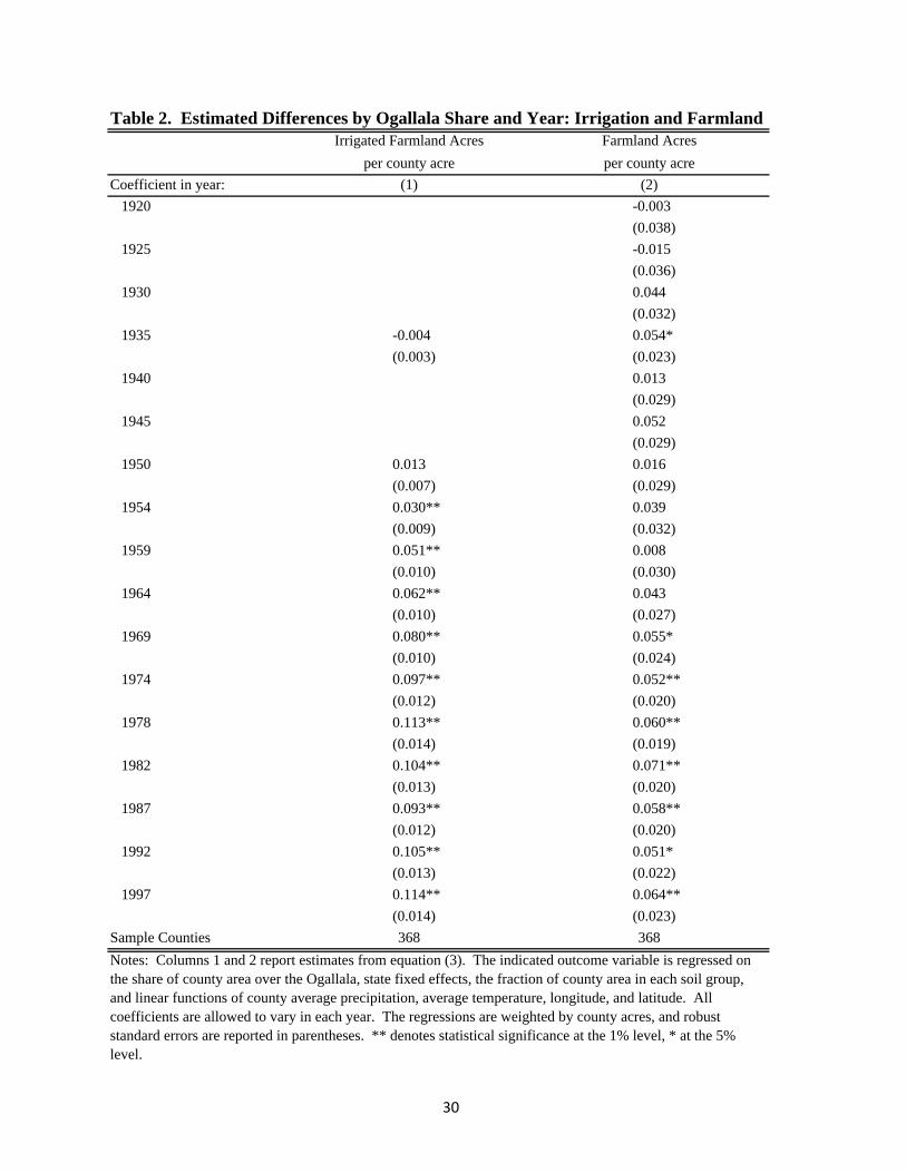
Table 2. Estimated Differences by Ogallala Share and Year: Irrigation and FarmlandIrrigated Farmland Acres Farmland Acres

per county acre per county acre

Coefficient in year: (1) (2)

1920 -0.003

(0.038)

1925 -0.015

(0.036)

1930 0.044

(0.032)

1935 -0.004 0.054*

(0.003) (0.023)

1940 0.013

(0.029)

1945 0.052

(0.029)

1950 0.013 0.016

(0.007) (0.029)

1954 0.030** 0.039

(0.009) (0.032)

1959 0.051** 0.008

(0.010) (0.030)

1964 0.062** 0.043

(0.010) (0.027)

1969 0.080** 0.055*

(0.010) (0.024)

1974 0.097** 0.052**

(0.012) (0.020)

1978 0.113** 0.060**

(0.014) (0.019)

1982 0.104** 0.071**

(0.013) (0.020)

1987 0.093** 0.058**

(0.012) (0.020)

1992 0.105** 0.051*

(0.013) (0.022)

1997 0.114** 0.064**

(0.014) (0.023)

Sample Counties 368 368

Notes: Columns 1 and 2 report estimates from equation (3). The indicated outcome variable is regressed on the share of county area over the Ogallala, state fixed effects, the fraction of county area in each soil group, and linear functions of county average precipitation, average temperature, longitude, and latitude. All coefficients are allowed to vary in each year. The regressions are weighted by county acres, and robust standard errors are reported in parentheses. ** denotes statistical significance at the 1% level, * at the 5% level.

30 

Table 3. Estimated Differences by Ogallala Share and Year: Corn and Wheat Acreages

Irrigated Corn All Corn Irrigated Wheat All WheatCoefficient in year: (1) (2) (3) (4)

1920 -0.0003 -0.0036 -0.0009 0.0108(0.0002) (0.0075) (0.0007) (0.0122)

1925 0.0108 0.0262*(0.0086) (0.0114)

1930 0.0112 0.0645**(0.0096) (0.0144)

1935 -0.0074* 0.0311**(0.0035) (0.0115)

1940

1945 0.0117 0.0340*(0.0081) (0.0136)

1950 0.0021* 0.0035 0.0012* 0.0733**(0.0010) (0.0080) (0.0006) (0.0139)

1954 0.0032** 0.0033 0.0016* 0.0340**(0.0012) (0.0069) (0.0006) (0.0105)

1959 0.0097** 0.0046 0.0035** 0.0515**(0.0026) (0.0075) (0.0012) (0.0099)

1964 0.0120** -0.0020 0.0072** 0.0264**(0.0027) (0.0052) (0.0017) (0.0095)

1969 0.0261**(0.0091)

1974 0.0332**(0.0115)

1978 0.0651** 0.0446** 0.0133** 0.0236*(0.0097) (0.0097) (0.0020) (0.0105)

1982 0.0578** 0.0381** 0.0187** 0.0315*(0.0094) (0.0090) (0.0026) (0.0125)

1987 0.0544** 0.0374** 0.0163** 0.0276**(0.0084) (0.0081) (0.0025) (0.0104)

1992 0.0670** 0.0499** 0.0171** 0.0156(0.0099) (0.0099) (0.0027) (0.0114)

1997 0.0762** 0.0652** 0.0140** 0.0146(0.0106) (0.0110) (0.0022) (0.0115)

Sample Counties 333 365 313 367

Corn Acres Harvestedper county acre

Wheat Acres Harvestedper county acre

Notes: Columns 1-4 report estimates from equation (3). The indicated outcome variable is regressed on the share of county area over the Ogallala, state fixed effects, the fraction of county area in each soil group, and linear functions of county average precipitation, average temperature, longitude, and latitude. All coefficients are allowed to vary in each year. The regressions are weighted by county acres, and robust standard errors are reported in parentheses. ** denotes statistical significance at the 1% level, * at the 5% level.

31

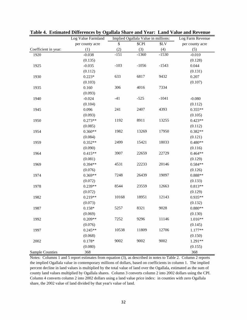
Table 4. Estimated Differences by Ogallala Share and Year: Land Value and RevenueLog Value Farmland Log Farm Revenue

per county acre $ $CPI $LV per county acreCoefficient in year: (1) (2) (3) (4) (5)

1920 -0.038 -151 -1360 -1530 -0.010(0.135) (0.128)

1925 -0.035 -103 -1056 -1543 0.044(0.112) (0.131)

1930 0.223* 633 6817 9432 0.207(0.103) (0.107)

1935 0.160 306 4016 7334

(0.093)1940 -0.024 -41 -525 -1041 -0.080

(0.104) (0.112)1945 0.096 241 2407 4393 0.355**

(0.093) (0.105)1950 0.273** 1192 8911 13255 0.423**

(0.085) (0.112)1954 0.360** 1982 13269 17950 0.382**

(0.084) (0.121)1959 0.352** 2499 15421 18033 0.480**

(0.090) (0.116)1964 0.415** 3907 22659 22729 0.464**

(0.081) (0.129)1969 0.394** 4531 22233 20146 0.584**

(0.076) (0.126)1974 0.369** 7248 26439 19097 0.888**

(0.072) (0.133)1978 0.239** 8544 23559 12663 0.813**

(0.072) (0.129)1982 0.219** 10168 18951 12143 0.935**

(0.073) (0.132)1987 0.158* 5257 8321 9028 0.880**

(0.069) (0.130)1992 0.209** 7252 9296 11146 1.016**

(0.076) (0.145)1997 0.245** 10538 11809 12706 1.177**

(0.068) (0.150)2002 0.178* 9002 9002 9002 1.291**

(0.080) (0.155)Sample Counties 368 368

Implied Ogallala Value in millions:

Notes: Columns 1 and 5 report estimates from equation (3), as described in notes to Table 2. Column 2 reports the implied Ogallala value in contemporary millions of dollars, based on coefficients in column 1. The implied percent decline in land values is multiplied by the total value of land over the Ogallala, estimated as the sum of county land values multiplied by Ogallala shares. Column 3 converts column 2 into 2002 dollars using the CPI. Column 4 converts column 2 into 2002 dollars using a land value price index: in counties with zero Ogallala share, the 2002 value of land divided by that year's value of land.

32

Table 5. Estimated Local Spillover Impacts: Nearby Non-Ogallala Counties vs. Counties 100km from the Ogallala Irrigated Log Farm Log Farm Farmland Farmland Irrigated Corn All Corn Irrigated All Wheat Value Revenue

Coefficient in: (1) (2) (3) (4) (5) (6) (7) (8)1920 0.134** -0.0002 0.0111 -0.00004 0.0249 0.277 0.210

(0.048) (0.0004) (0.0179) (0.00059) (0.0176) (0.172) (0.184)1935 0.000 0.092 0.0086 0.0119 0.285

(0.006) (0.056) (0.0111) (0.0133) (0.213)1945 0.009 0.0162 0.0176 0.268 0.232

(0.054) (0.0203) (0.0176) (0.189) (0.187)1950 -0.002 -0.048 0.0008 0.0182 -0.00020 -0.0029 0.085 0.054

(0.009) (0.049) (0.0016) (0.0202) (0.00022) (0.0213) (0.138) (0.170)1954 -0.001 -0.044 0.0017 0.0091 -0.00016 0.0041 0.0754 -0.036

(0.009) (0.060) (0.0017) (0.0189) (0.00013) (0.0157) (0.159) (0.194)1959 -0.005 -0.016 0.0036 0.0078 -0.00020 0.0153 0.102 0.007

(0.010) (0.051) (0.0037) (0.0206) (0.00019) (0.0144) (0.115) (0.192)1964 -0.004 -0.030 0.0037 -0.0012 -0.00004 0.0004 0.061 0.020

(0.010) (0.050) (0.0031) (0.0148) (0.00043) (0.0142) (0.118) (0.209)1969 -0.002 0.021 0.0022 0.073 0.111

(0.010) (0.043) (0.0164) (0.117) (0.223)1978 0.003 0.018 0.0102 0.0068 -0.00024 0.0122 -0.022 0.204

(0.013) (0.049) (0.0076) (0.0162) (0.00085) (0.0208) (0.122) (0.257)1982 0.003 0.019 0.0083 0.0054 -0.00003 -0.0059 -0.015 0.234

(0.012) (0.053) (0.0083) (0.0154) (0.00116) (0.0244) (0.144) (0.235)1987 0.000 0.036 0.0065 0.0044 -0.00004 -0.0042 -0.042 0.181

(0.010) (0.047) (0.0062) (0.0129) (0.00083) (0.0199) (0.106) (0.262)1992 0.004 0.042 0.0104 0.0066 0.00002 -0.0011 0.117 0.298

(0.012) (0.056) (0.0087) (0.0160) (0.00114) (0.0222) (0.116) (0.277)1997 -0.001 -0.004 0.0081 0.0049 -0.00066 -0.0215 0.078 0.190

(0.012) (0.052) (0.0070) (0.0145) (0.00176) (0.0217) (0.119) (0.271)Sample Counties 136 136 114 133 99 135 136 136

Corn Acres Harvested Wheat Acres Harvested

Notes: For counties with zero area over the Ogallala, each column reports estimates from a modified equation (3): coefficients report the impact of "Negative Distance to Ogallala Boundary," measured in 100km units. Coefficients reflect average outcomes in counties next to the Ogallala boundary, relative to counties 100km away. Otherwise, the specifications are as described in Tables 2-4. For conciseness, some coefficients are omitted from 1925, 1930, 1940, 1974, and 2002. ** denotes statistical significance at the 1% level, * at the 5% level.

33 

Table 6. Estimated Impacts of Ogallala and Drought on Yields, Relative to 1940 - 1956(1) (2) (3)

Panel A. Log Corn Yield

Ogallala * Drought * (1958 - 1975) 0.375** 0.353** 0.292*

(0.101) (0.098) (0.121)

Ogallala * Drought * (1976 - 1993) 0.077* -0.050 -0.036

(0.038) (0.065) (0.080)

Ogallala * (1958 - 1975) -0.034 -0.023 -0.053

(0.145) (0.151) (0.151)

Ogallala * (1976 - 1993) 0.084 0.082 0.082

(0.139) (0.137) (0.139)

Sample Counties 134 134 134

Panel B. Log Wheat Yield

Ogallala * Drought * (1958 - 1975) 0.008 0.075 0.067

(0.052) (0.045) (0.054)

Ogallala * Drought * (1976 - 1993) 0.057 0.045 -0.024

(0.055) (0.057) (0.076)

Ogallala * (1958 - 1975) 0.052 0.047 0.046

(0.042) (0.042) (0.042)

Ogallala * (1976 - 1993) 0.094 0.074 0.060

(0.072) (0.073) (0.075)

Additional Controls:

Drought * County Fixed Effects Yes Yes Yes

Drought * Era Yes Yes Yes

Drought * Era * State & Soil No Yes Yes

Drought * Era * Climate & X/Y No No Yes

Sample Counties 165 165 165

Notes: Columns 1-3 report estimates from versions of equation (4). In panel A, log corn yield is regressed on the triple interaction between a county's Ogallala share, normalized Palmer Drought Severity Index, and a dummy for the second era (1958 - 1975) or third era (1976 - 1993). Also reported is the double interaction between Ogallala share and era. All specifications control for county fixed effects and era-specific controls for state, soil group, and linear functions of average precipitation, average temperature, longitude, and latitude. In addition, all specifications control for interactions between drought and county fixed effects and interactions between drought and era fixed effects. The sample is limited to 134 counties in Nebraska, South Dakota, and Iowa with data available in each of the 54 years between 1940 and 1993. Column 2 also controls for interactions between drought and state fixed effects and interactions between drought and soil group shares. Column 3 also controls for interactions between drought and linear functions of average precipitation, average temperature, longitude, and latitude. Panel B reports estimated impacts on wheat yields. The sample is limited to 165 counties in Colorado, Kansas, Oklahoma, South Dakota, and Wyoming with wheat yield data in each of the 54 years between 1940 and 1993. The regressions are weighted by county acres, and robust standard errors are reported in parentheses. ** denotes statistical significance at the 1% level, * at the 5% level.

34

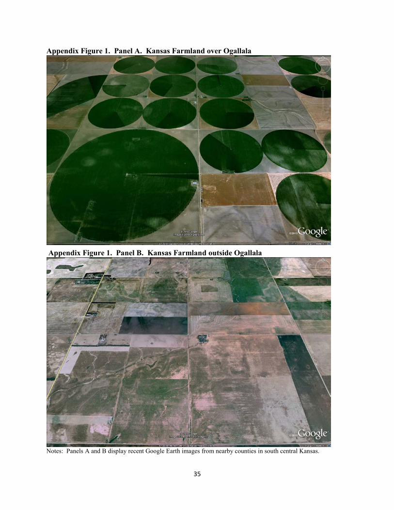
35

Appendix Figure 1. Panel A. Kansas Farmland over Ogallala

Appendix Figure 1. Panel B. Kansas Farmland outside Ogallala

Notes: Panels A and B display recent Google Earth images from nearby counties in south central Kansas.

36

Appendix Figure 2. Ogallala Boundary and Natural Vegetation Regions

Notes: The Ogallala boundary (USGS) is overlaid with natural vegetation regions, as mapped by the 1924 Atlas of Agriculture (USDA 1924).

VIII Theory Appendix

This appendix contains proofs of the theoretical results discussed in section II.

VIII.A Model Setup

The maximization problem of our representative farmer is

maxL1,L2,w1,w2

y1(L1, w1, d) + y2(L2, w2, d)

subject to the constraints

w1 + w2 = w̄

L1 + L2 = L̄

The production functions are globally concave, with five additional assumptions:

1. The marginal product of water is higher for the first crop:

∂y1/∂w1 > ∂y2/∂w2 > 0.

2. The marginal product of water declines slower for the first crop:

∂2y2/(∂w2)2 < ∂2y1/(∂w1)

2 < 0.

3. Water and land are complementary for both crops, but weakly more so for the first

crop:

∂2y1/∂L1∂w1 ≥ ∂2y2/∂L2∂w2 > 0.

4. Drought decreases the productivity of land for both crops, but drought has a larger

negative effect on the water-intensive crop:

∂2y1/∂L1∂d < ∂2y2/∂L2∂d < 0.

5. Drought increases the productivity of water for both crops, but more so for the water-

intensive crop:

∂2y1/∂w1∂d > ∂2y2/∂w2∂d > 0.

37

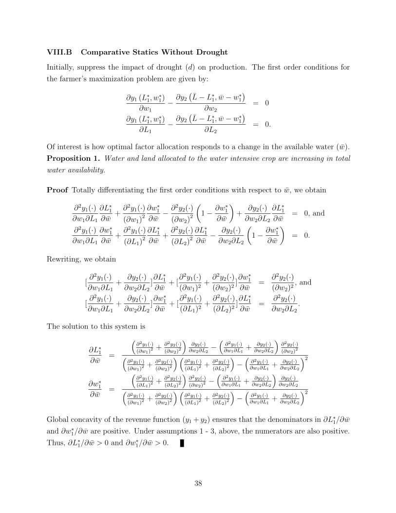
VIII.B Comparative Statics Without Drought

Initially, suppress the impact of drought (d) on production. The first order conditions for

the farmer’s maximization problem are given by:

∂y1 (L∗1, w

∗1)

∂w1

−∂y2

(L̄− L∗

1, w̄ − w∗1

)∂w2

= 0

∂y1 (L∗1, w

∗1)

∂L1

−∂y2

(L̄− L∗

1, w̄ − w∗1

)∂L2

= 0.

Of interest is how optimal factor allocation responds to a change in the available water (w̄).

Proposition 1. Water and land allocated to the water intensive crop are increasing in total

water availability.

Proof Totally differentiating the first order conditions with respect to w̄, we obtain

∂2y1(·)∂w1∂L1

∂L∗1

∂w̄+∂2y1(·)(∂w1)

2

∂w∗1

∂w̄− ∂2y2(·)

(∂w2)2

(1− ∂w∗

1

∂w̄

)+

∂y2(·)∂w2∂L2

∂L∗1

∂w̄= 0, and

∂2y1(·)∂w1∂L1

∂w∗1

∂w̄+∂2y1(·)(∂L1)

2

∂L∗1

∂w̄+∂2y2(·)(∂L2)

2

∂L∗1

∂w̄− ∂y2(·)∂w2∂L2

(1− ∂w∗

1

∂w̄

)= 0.

Rewriting, we obtain

[∂2y1(·)∂w1∂L1

+∂y2(·)∂w2∂L2

]∂L∗

1

∂w̄+ [

∂2y1(·)(∂w1)2

+∂2y2(·)(∂w2)2

]∂w∗

1

∂w̄=

∂2y2(·)(∂w2)2

, and

[∂2y1(·)∂w1∂L1

+∂y2(·)∂w2∂L2

]∂w∗

1

∂w̄+ [

∂2y1(·)(∂L1)2

+∂2y2(·)(∂L2)2

]∂L∗

1

∂w̄=

∂2y2(·)∂w2∂L2

.

The solution to this system is

∂L∗1

∂w̄=

(∂2y1(·)(∂w1)

2 + ∂2y2(·)(∂w2)

2

)∂y2(·)∂w2∂L2

−(

∂2y1(·)∂w1∂L1

+ ∂y2(·)∂w2∂L2

)∂2y2(·)(∂w2)

2(∂2y1(·)(∂w1)

2 + ∂2y2(·)(∂w2)

2

)(∂2y1(·)(∂L1)

2 + ∂2y2(·)(∂L2)

2

)−(

∂2y1(·)∂w1∂L1

+ ∂y2(·)∂w2∂L2

)2∂w∗

1

∂w̄=

(∂2y1(·)(∂L1)

2 + ∂2y2(·)(∂L2)

2

)∂2y2(·)(∂w2)

2 −(

∂2y1(·)∂w1∂L1

+ ∂y2(·)∂w2∂L2

)∂y2(·)∂w2∂L2(

∂2y1(·)(∂w1)

2 + ∂2y2(·)(∂w2)

2

)(∂2y1(·)(∂L1)

2 + ∂2y2(·)(∂L2)

2

)−(

∂2y1(·)∂w1∂L1

+ ∂y2(·)∂w2∂L2

)2Global concavity of the revenue function (y1 + y2) ensures that the denominators in ∂L∗

1/∂w̄

and ∂w∗1/∂w̄ are positive. Under assumptions 1 - 3, above, the numerators are also positive.

Thus, ∂L∗1/∂w̄ > 0 and ∂w∗

1/∂w̄ > 0.

38

VIII.C General Case: Comparative Statics With Drought

Proposition 2. When the land allocation is held constant, an increase in water availability

reduces the (negative) impact of drought:

d

dw̄

[∂y1 (L∗

1, w∗1 (w̄) , d)

∂d+∂y2 (L∗

2, w∗2 (w̄) , d)

∂d

]> 0.

Conversely, when the land allocation can respond to changes in w̄, an increase in water

availability has an ambiguous effect on the impact of drought.

Proof Consider the effect of w̄ on the derivative of the revenue function with respect to d.

d

dw̄

[∂y1∂d

+∂y2∂d

]=

∂2y1∂d∂L1

∂L∗1

∂w̄+

∂2y1∂d∂w1

∂w∗1

∂w̄− ∂2y2∂d∂L2

∂L∗1

∂w̄+

∂2y2∂d∂w2

∂w∗2

∂w̄

=

(∂2y1∂d∂w1

∂w∗1

∂w̄+

∂2y2∂d∂w2

∂w∗2

∂w̄

)︸ ︷︷ ︸

>0

+

(∂2y1∂d∂L1

− ∂2y2∂d∂L2

)∂L∗

1

∂w̄︸ ︷︷ ︸<0

Assumption 5 and Proposition 1 imply that the first term is positive. Assumption 4 and

Proposition 1 imply that the second term is negative. Thus, an increase in water availability

has an ambiguous effect on the impact of drought. If the land allocation is held fixed

(∂L∗1/∂w̄ = 0), then the impact is unambiguously positive. In addition, the effect of water

availability on the impact of drought is more positive than when the land allocation is free

to adjust.

VIII.D Special Case: Comparative Statics With Drought

Consider the special case of constant returns to land, in which the farmer maximizes

L1y1(w1, d) + L2y2(w2, d).

Proposition 3. When the production technology displays constant returns to land:

1. If the land allocation can adjust to w̄, then an increase in water availability increases

the (negative) impact of drought:

d

dw̄

[L∗1 (w̄)

∂y1 (w∗1 (w̄) , d)

∂d+ L∗

2 (w̄)∂y2 (w∗

2 (w̄) , d)

∂d

]< 0.

2. If the land allocation is fixed, then an increase in water availability reduces the (nega-

tive) impact of drought.

39

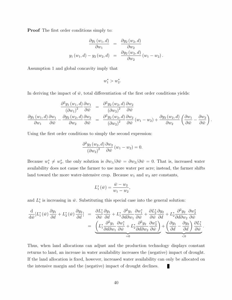
Proof The first order conditions simply to:

∂y1 (w1, d)

∂w1

=∂y2 (w2, d)

∂w2

y1 (w1, d)− y2 (w2, d) =∂y2 (w2, d)

∂w2

(w1 − w2) .

Assumption 1 and global concavity imply that

w∗1 > w∗

2.

In deriving the impact of w̄, total differentiation of the first order conditions yields:

∂2y1 (w1, d)

(∂w1)2

∂w1

∂w̄=

∂2y2 (w2, d)

(∂w2)2

∂w2

∂w̄

∂y1 (w1, d)

∂w1

∂w1

∂w̄− ∂y2 (w2, d)

∂w2

∂w2

∂w̄=

∂2y2 (w2, d)

(∂w2)2

∂w2

∂w̄(w1 − w2) +

∂y2 (w2, d)

∂w2

(∂w1

∂w̄− ∂w2

∂w̄

).

Using the first order conditions to simply the second expression:

∂2y2 (w2, d)

(∂w2)2

∂w2

∂w̄(w1 − w2) = 0.

Because w∗1 6= w∗

2, the only solution is ∂w1/∂w̄ = ∂w2/∂w̄ = 0. That is, increased water

availability does not cause the farmer to use more water per acre; instead, the farmer shifts

land toward the more water-intensive crop. Because w1 and w2 are constants,

L∗1 (w̄) =

w̄ − w2

w1 − w2

,

and L∗1 is increasing in w̄. Substituting this special case into the general solution:

d

dw̄[L∗

1 (w̄)∂y1∂d

+ L∗2 (w̄)

∂y2∂d

] =∂L∗

1

∂w̄

∂y1∂d

+ L∗1

∂2y1∂d∂w1

∂w∗1

∂w̄+∂L∗

2

∂w̄

∂y2∂d

+ L∗2

∂2y2∂d∂w2

∂w∗2

∂w̄

=

(L∗1

∂2y1∂d∂w1

∂w∗1

∂w̄+ L∗

2

∂2y2∂d∂w2

∂w∗2

∂w̄

)︸ ︷︷ ︸

=0

+

(∂y1∂d− ∂y2

∂d

)∂L∗

1

∂w̄︸ ︷︷ ︸<0

.

Thus, when land allocations can adjust and the production technology displays constant

returns to land, an increase in water availability increases the (negative) impact of drought.

If the land allocation is fixed, however, increased water availability can only be allocated on

the intensive margin and the (negative) impact of drought declines.

40