The historic nor’easter of 13-14 March 2010 By

Richard H. Grumm National Weather Service

1. INTRODUCTION

An historic nor’easter affected the East Coast of the United States on 13-14 March 2010. The storm will be remembered for heavy rainfall (Fig. 1), flooding, strong winds, and the coastal surge1. Hurricane force wind gusts were reported at Kennedy International Airport (KJFK) around 0000 UTC 14 March 2010 when wind gusts reach 64KTS (74 mph). Islip had 54 KTS winds2

This storm has been compared to several past storms. The nor’easters of 12-13 December 1992 and 07-08 January 1996 storms both produced strong storm surges along the East Coast. Unlike this storm, these storms produced areas of heavy snowfall. Another similar storm, which produced heavy rainfall, was the 3-4 March 1993 event. All of these storms had strong easterly winds with significant u-wind anomalies north of the cyclone. It was in this general area where these storms produced the most significant impact. The 850 hPa winds and u-wind anomalies during the peak of the 13-14 March 2010 nor’easter are shown in Figure 2.

. The strong winds produced widespread power outages, downed trees, and produced coastal flooding due to a strong storm surge.

Colle et al (2010) examined storms which produced storm surges in New York City. They listed all storms which produced storms which produced significant surges above the mean-high water mark (Colle et al. 2010: Table 1) separating out tropical cyclones (Tab le2: Colle et al. 2010). The top 3 storms were Hurricane 1 Information provided by Brian Colle SUNY-Stony Brook.

2 KISP 132356Z 08027G42KT 4SM RA BKN010 OVC016 09/07 A2958 RMK AO2 PK WND 10054/2312 SLP017 P0008 60042 T00940067 10094 20089 58017 $=

Gloria September 1985 (2.0m), Hurricane Donna September 1960 (1.73m), and the nor’easter of 12-13 December 1992 (1.75m). A total of 17 tropical storms produced strong storm surges. The list of extratropical cyclones includes many memorable East Coast Winter Storms (ECWS) and famous nor’easters including the 31 October 1991 (1.40m), 13 March 1993 “Superstorm” (1.46m), and the 7-8 January 1996 “Blizzard of 1996” (1.35m) and the 14-15 November 1995 nor’easter (1.24). Storm surges and coastal flooding are often overlooked but important aspect nor’easters. The storm of 13-14 March produced a surge of 1.28 m.

As with many nor’easters, this storm produced high winds. The highest gusts were on Long Island including KJFK (75 mph) and Breezy Points (66 mph). Table 1 lists some of the higher winds reports for the event for gusts over 50 MPH. The strongest winds were primarily along the coast. However, strong winds and wind damage were reported well into central Pennsylvania.

This event also produced locally heavy rainfall. Coastal areas received 2 to 3 inches with locally higher amounts exceeding 5 inches. A higher elevation report in southern Pennsylvania received 6.25 inches of rainfall. Table 2 lists rainfall amounts in excess of 5 inches. There were over 165 reports of 3 inches or more observed liquid equivalent precipitation.

This paper will provide an overview of the historic nor’easter of 13-14 March 2010. The focus is on the pattern and the significant weather impacts. A comparison of this storm to several notable nor’easters from the published literature is presented too.

2. METHODS AND DATA

The 500 hPa heights, 850 hPa temperatures and winds, other standard level fields were derived

from the NCEP GFS, GEFS, and the NCEP/NCAR (Kalnay et al. 1996) reanalysis data. The means and standard deviations used to compute the standardized anomalies were from the NCEP/NCAR data as described by Hart and Grumm (2001). Anomalies were displayed in standard deviations from normal, as standardized anomalies. All data were displayed using GrADS (Doty and Kinter 1995).

The standardized anomalies computed as:

SD = (F – M)/σ ()

Where F is the value from the reanalysis data at each grid point, M is the mean for the specified date and time at each grid point and σ is the value of 1 standard deviation at each grid point.

Model and ensemble data shown here were primarily limited to the GFS and GEFS. The 1.25x1.25 degree JMA data may be used when it becomes available. The NAM and SREF data were also available for use in this study. Displays will focus on the observed pattern and some forecast issues associated with the pattern.

For brevity, times will be displayed in day and

Figure 1 Total observed liquid precipitation (mm) from 1200 UTC 12 March through 1200 UTC 15 March 2010. From the unified precipitation data set. Return to analysis section.

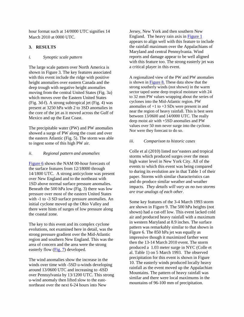
hour format such at 14/0000 UTC signifies 14 March 2010 at 0000 UTC.

3. RESULTS i. Synoptic scale pattern The large scale pattern over North America is shown in Figure 3. The key features associated with this event include the ridge with positive height anomalies over eastern Canada and the deep trough with negative height anomalies moving from the central United States (Fig. 3a) which moves over the Eastern United States (Fig. 3d-f). A strong subtropical jet (Fig. 4) was present at 3250 hPa with 2 to 3SD anomalies in the core of the jet as it moved across the Gulf of Mexico and up the East Coast. The precipitable water (PW) and PW anomalies showed a surge of PW along the coast and over the eastern Atlantic (Fig. 5). The storm was able to ingest some of this high PW air.

ii. Regional pattern and anomalies Figure 6 shows the NAM 00-hour forecasts of the surface features from 12/18000 through 14/1800 UTC. A strong anticyclone was present over New England and to the northeast with 1SD above normal surface pressure anomalies. Beneath the 500 hPa low (Fig. 3) there was low pressure over most of the eastern United States with -1 to -3 SD surface pressure anomalies. An initial cyclone moved up the Ohio Valley and there were hints of surges of low pressure along the coastal zone. The key to this event and its complex cyclone evolutions, not examined here in detail, was the strong pressure gradient over the Mid-Atlantic region and southern New England. This was the area of concern and the area were the strong easterly flow (Fig. 7) developed. The wind anomalies show the increase in the winds over time with -5SD u-winds developing around 13/0600 UTC and increasing to -6SD over Pennsylvania by 13/1200 UTC. This strong u-wind anomaly then lifted slow to the east-northeast over the next 6-24 hours into New

Jersey, New York and then southern New England. The heavy rain axis in Figure 1 appears to align well with this feature to include the rainfall maximum over the Appalachians of Maryland and central Pennsylvania. Wind reports and damage appear to be well aligned with this feature too. The strong easterly jet was a critical player in this event.

A regionalized view of the PW and PW anomalies is shown in Figure 8. These data show that the strong southerly winds (not shown) in the warm sector taped some deep tropical moisture with 24 to 32 mm PW values wrapping about the series of cyclones into the Mid-Atlantic region. PW anomalies of +1 to +3 SDs were present in and near the region of heavy rainfall. This is best seen between 13/0600 and 14/0000 UTC. The really deep moist air with +5SD anomalies and PW values over 50 mm never surge into the cyclone. Nor were they forecast to do so.

iii. Comparison to historic cases Colle et al (2010) listed nor’easters and tropical storms which produced surges over the mean high water level in New York City. All of the events to which this event was being compared to during its evolution are in that Table 1 of their paper. Storms with similar characteristics can and do produce similar weather and weather impacts. They details will vary as no two storms are true analogs of each other. Some key features of the 3-4 March 1993 storm are shown in Figure 9. The 500 hPa heights (not shown) had a cut-off low. This event lacked cold air and produced heavy rainfall with a maximum in western Maryland at 8.9 inches. The surface pattern was remarkably similar to that shown in Figure 6. The 850 hPa jet was equally as impressive though it maximized farther west then the 13-14 March 2010 event. The storm produced a 1.03 meter surge in NYC (Colle et al. Table 1) on 5 March 1993. The observed precipitation for this event is shown in Figure 10. The easterly winds produced locally heavy rainfall as the event moved up the Appalachian Mountains. The pattern of heavy rainfall was similar and there were local maximums in the mountains of 96-100 mm of precipitation.

Another similar event, which caused massive coastal storm surge and flooding issues (Colle et al 2010), was the storm of 11-13 December 1992 (Fig. 11). This storm was associated with cold air and there was some extremely heavy snowfall (2 to 3 feet) in the mountains of Maryland and Pennsylvania. This slow moving storm produced a similar Appalachian precipitation maximum and really produced heavy rainfall in eastern New England (Fig. 12). The pattern was shown at 12/1800 UTC as the rain began in earnest in New England. However, between 11/1800 and 12/0000 UTC a -5SD u-wind anomaly moved through Maryland and Pennsylvania (not shown). The 7-8 January 1996 or Blizzard of 1996 storm was also similar to this storm. Obviously the storm contained cold air and was snow producing nor’easter. The data here are valid at 08/0600 UTC as the surge in NYC peaked around 08/0600 UTC (Colle et al. 2010). This storm had an organized and deep cyclone (Fig 13c) and of course the strong and anomalous u-wind anomalies (Fig 13a). This event was faster moving and associated with colder air and thus produced lower overall precipitation amounts (Figure 14). iv. Forecasts The event was well predicted by the NCEP models and ensemble forecast systems (EFS). As with all events there were timing and location issues which impact the forecasts.

The GEFS forecasts of 1 inch or greater QPF from 1200 UTC 09-11 March 2010 are shown in Figure 15. These data show that with considerable lead time the potential for heavy rain were predicted for the general region where heavy rain was observed. Other probability forecasts produced similar outcomes using 2 inches and 36 hour accumulations.

In general the rain event and affected are was well predicted. The 9 forecasts of the ensemble mean QPF (Fig. 16) further support this general

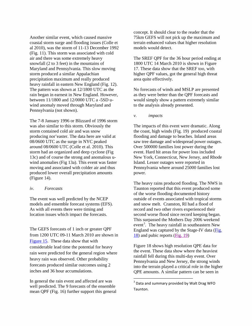
concept. It should clear to the reader that the 75km GEFS will not pick up the maximum and terrain enhanced values that higher resolution models would detect. The SREF QPF for the 36 hour period ending at 1800 UTC 14 March 2010 is shown in Figure 17. These data show that the SREF too, with higher QPF values, got the general high threat area quite effectively. No forecasts of winds and MSLP are presented as they were better than the QPF forecasts and would simply show a pattern extremely similar to the analysis already presented. v. impacts The impacts of this event were dramatic. Along the coast, high winds (Fig. 19) produced coastal flooding and damage to beaches. Inland areas saw tree damage and widespread power outages. Over 500000 families lost power during the event. Hard hit areas for power loss included New York, Connecticut, New Jersey, and Rhode Island. Lesser outages were reported in Pennsylvania where around 25000 families lost power. The heavy rains produced flooding. The NWS in Taunton reported that this event produced some of the worse flooding documented history outside of events associated with tropical storms and snow melt. Cranston, RI had a flood of record and two other rivers experienced their second worse flood since record keeping began. This surpassed the Mothers Day 2006 weekend event3

Fig. 18

. The heavy rainfall in southeastern New England was captured by the Stage-IV data (

) and pubic reports (Fig. 19) Figure 18 shows high resolution QPE data for the event. These data show where the heaviest rainfall fell during this multi-day event. Over Pennsylvania and New Jersey, the strong winds into the terrain played a critical role in the higher QPE amounts. A similar pattern can be seen in 3 Data and summary provided by Walt Drag WFO Taunton.

New England. Both regions showed clear and consistent rain shadows. The Connecticut and Hudson Valleys show up as clear rainfall minimums in the lower panel of Figure 18. A similar minimum was present west of the Catskills. In the upper panel, the Susquehanna Valley and the lee, for easterlies, of the Alleghenies were also precipitation minimums. 4. CONCLUSIONS

A slow moving cyclone produced an historic nor’easter on 13-14 March 2010. This storm produced hurricane force wind gusts, high surge, a storm surge, and heavy rainfall. The winds produced widespread power outages due to downed trees and wires. The winds also impacted coastal regions. The rains were intense and produced flooding in Pennsylvania, New York, New Jersey and New England. This was a high impact event that contained clear and consistent signals in the NCEP models and EFS to provide a reasonable lead-time on predicting this event. This storm shared main of the characteristics of many of the significant storms of the winter of 2009-2010. The deep trough moving beneath the high latitude ridge is a common theme for nor’easters and was the case with this event. This storm lacked cold air and did not produce significant snowfall. Additionally, this storm had strong southern stream jet (Fig. 4) which is quite common during an ENSO positive winter. Another feature of many strong cyclonic events was the surge of high PW air (Fig. 5) into the cyclone.

The storm produced high winds with many locations along the coast having near hurricane forecast winds. Over 500,000 people lost power mainly along the coastal zone during the event. The strong winds and coastal flooding appeared to be timed well and linked to the anomalous low-level easterly jet (Fig. 7). This jet was also well timed and coincided with the storm surge and surf which caused flooding in NYC and adjacent New Jersey and along the coast of southern New England as it lifted to the north and east.

Heavy rains were another issue, though they were not focused over areas with large snow water and the rains came over a long period of time. This and slow steady snow melt for several days ahead of the event precluded major and widespread flooding. Many dodged a bullet. The axis of heavy rainfall (Fig. 1) was well aligned with the anomalous low-level jet and u-wind anomalies as shown in Figure 7. Overall, both the SREF and GEFS did well predicting the rainfall. Due to resolution issues they lacked, though the SREF hinted at, the impact and localization of the terrain.

During the event, high resolution windows from the GFS were used (not shown) to produce QPFs for the time of heavy rainfall over Pennsylvania. The results of these downscaled GFS runs to 8 km produced heavy rainfall in many of the terrain focused areas where the rain fell. Due to uncertainty issues, some of the regions of heavy rainfall from downscaled runs 60, 66 and 72 hours in advance did not materialize. But this real-time test showed the value of downscaled runs during periods of heavy rainfall events.

The comparative nor’easter shown here all shared some common characteristics. The key feature they all had in common was strong 850 hPa u-winds with u-wind anomalies in the -5 to -6SD range. These common features, often well predicted could be leveraged to improve rating and evaluating East Coast Winter storms. Ensemble forecasts compared to climatology and model climatologies could be leveraged to rate nor’easters based on ensemble forecasts. An operational storm rating system from 1 to 5 could be used. Threats for key features could be made in relation to snowfall threats, rainfall threats, high surf and coastal flooding threats and high wind threats. This approach would eliminate some of the adjectives used to describe storms.

The time to produce products to rate and show key threats has passed we need such products to evaluate significant threats with discrete probabilities now.

Clearly, we need to better leverage EFS data to rate storms and provide probabilistic threat outcomes. These products need to be made available to NWS forecasters to facilitate rapid identification of key meteorological threats. Both planview and point specific displays must be provided to forecasters.

5. Acknowledgements

Discussion on ensemble displays were conducted before the event with Lance Bosart, SUNY-Albany. Tim Hewson provided ECMWF guidance related to the storm to include ECMWF EFI forecasts for New York City. Local support and data summaries were provided by the local NWS Office in State College. Thanks to my old friend John LaCorte for decoding and plotting rain, snow, and wind reports.

6. REFERENCES

Colle, B.A., F. Buonaiuto, M.J. Bowman, R.E. Wilson, R. Flood, R. Hunter, A. Mintz, and D. Hill, 2008: New York City's Vulnerability to Coastal Flooding. Bull. Amer. Meteor. Soc., 89, 829-841.’

Colle, B.A., K. Rojowsky, and F. Buonaiuto, 2010: New York City Storm Surges: Climatology and an Analysis of the Wind and Cyclone Evolution. J.Appl. Meteor. Climatol., 49, 85-100.

Doswell,C.A.,III, H.E Brooks and R.A. Maddox, 1996: Flash flood forecasting: An ingredients based approach. Wea. Forecasting, 11, 560-581.

Doty, B. E., and J. L. Kinter III, 1995: Geophysical data and visualization using GrADS. Visualization Techniques Space and Atmospheric Sciences, E. P. Szuszczewicz and Bredekamp, Eds., NASA, 209–219.

Grumm, R.H. and R. Hart. 2001: Standardized Anomalies Applied to Significant Cold Season Weather

Events: Preliminary Findings. Wea. and Fore., 16,736–754.

Grumm, R.H., and R. Hart, 2001a: Anticipating Heavy Rainfall: Forecast Aspects. Preprints, Symposium on Precipitation Extremes, Albuquerque, NM, Amer. Meteor. Soc., 66-70.

Grumm, R.H., and R. Holmes, 2007: Patterns of heavy rainfall in the mid-Atlantic. Pre-prints, Conference on Weather Analysis and Forecasting,Park City, UT, Amer. Meteor. Soc., 5A.2.

Grumm, Richard H. 2000, "Forecasting the Precipitation Associated with a Mid-Atlantic States Cold Frontal Rainband", NWA Digest,24, 37-51.

Hart, R. E., and R. H. Grumm, 2001: Using normalized climatological anomalies to rank synoptic scale events objectively. Mon. Wea. Rev., 129, 2426–2442.

Junker, N.W., R.H. Grumm,R.H. Hart, L.F Bosart, K.M. Bell, and F.J. Pereira, 2008: Use of normalized anomaly fields to anticipate extreme rainfall in the mountains of northern California.Wea. Forecasting, 23,336-356.

--------, M.J. Brennan, F. Pereira, M.J. Bodner, and R.H. Grumm, 2009: Assessing the Potential for Rare Precipitation Events with Standardized Anomalies and Ensemble Guidance at the Hydrometeorological Prediction Center. Bull. Amer. Meteor. Soc., 90, 445–453.

Lackmann, G. M., and J. R. Gyakum, 1999: Heavy cold-season precipitation in the northwestern United States: Synoptic climatology and an analysis of the flood of 17–18 January 1986. Wea. Forecasting, 14, 687–700.

Neiman, P.J., F.M. Ralph, A.B. White, D.E. Kingsmill, and P.O.G. Persson, 2002: The Statistical Relationship between Upslope Flow and Rainfall in California's Coastal Mountains: Observations during CALJET. Mon. Wea. Rev., 130, 1468–1492.

______ , _____, G.A. Wick, J.D. Lundquist,

and M.D. Dettinger, 2008: Meteorological Characteristics and

Overland Precipitation Impacts of Atmospheric Rivers Affecting the West Coast of North America Based on Eight Years of SSM/I Satellite Observations. J. Hydrometeor., 9, 22–47.

Stuart, N.A., and R.H. Grumm, 2006: Using

Wind Anomalies to Forecast East Coast Winter Storms. Wea. Forecasting, 21, 952–968.

Figure 2. GFS 00-hour forecasts showing 850 hPa winds (KTS) and 850 hPa wind anomalies. Data are valid at a) 0000 UTC 13 March, b) 0600 UTC 13 March, c) 1200 UTC 13 March, d) 1800 UTC 13 March, e) 0000 UTC 14 March, and f) 0600 UTC UTC 14 March 2010

Figure 3. As in Figure 2 except for 500 hPa heights (m) and height anomalies over North America.

Figure 4. As in Figure 2 except 250 hPa winds and 250 hPa wind anomalies.

Figure 5. As in Figure 2 except for precipitable water (mm) and precipitable water anomalies. Return to text.

Figure 6. NAM 00-hour forecasts of mean-sea level pressure (hPa) and pressure anomalies. The data shown are form 00-hour NAM initialized at at a) 1800 UTC 12 March, b) 0000 UTC 13 March, c) 0600 UTC 13 March, d) 1200 UTC 13 March, e) 1800 UTC 13 March, f) 0000 UTC 14 March, g) 0600 UTC 14 March, h)1200 UTC 14 March, and i) 1800 UTC 14 March 2010.

Figure 7. As in Figure 6 except for NAM 850 hPa winds (kts) and u-wind anomalies. Winds have been thinned showing every 3rd grib point.

Figure 8. As in Figures 6 & 7 except for NAM PW and PW anomalies. Return to text.

Figure 9. JRA analysis with NCEP/NCAR bases anomalies of conditions at 1800 UTC 04 March 1993 showing a) 850 hPa u-winds and u-wind anomalies, b) 850 hPa v-winds and v-wind anomalies, c) mean sea level pressure and anomalies, and d) precipitable water and anomalies.

Figure 10. As in Figure 1 except for 1200 UTC 3-6 March 1993.

Figure 11. As in Figure 9 except valid at 1800 UTC 12 December 1992.

Figure 12. As in Figure 10 except valid for 1200 UTC 10-13 December 1992.

Figure 13. As in Figure 9 except valid at 0600 UTC 8 January 1996.

KJFK 132351Z 08035G64KT 5SM -RA BR BKN014 OVC021 09/07 A2949 RMK AO2 PK WND 07064/2347 SLP986 P0000 60033 T00940072 10111 20094 56026 KJFK 132351Z 08035G64KT 5SM -RA BR BKN014 OVC021 09/07 A2949 KJFK 140051Z 09035G48KT 10SM -RA BKN014 OVC020 11/08 A2952 RMK AO2 PK WND 08055/0041 SLP995 P0001 T01060078

Figure 14. As in Figure 9 except valid 1200 UTC 6 to 1200 UTC 9 January 1996.

Town State Wind MPH LST AM/PM

NYC/JFK ARPT NY 75 833 PM EAST MILTION MA 69 1251 AM JONES BEACH STATE NY 67 350 PM BREEZY POINT NY 67 330 PM BLUE POINT NY 67 302 PM FIRE ISLAND NY 67 700 PM FORT LEE NJ 66 634 PM AMITY HARBOR NY 66 621 PM BAYVILLE NY 63 435 PM JONES BEACH ISLAND NY 63 240 PM WHITE PLAINS NY 62 629 PM FARMINGDALE NY 60 636 PM GROTON/NEW LONDON CT 59 812 PM TETERBORO NJ 59 859 PM SHIRLEY NY 56 340 PM SHIRLEY NY 56 539 PM YARMOUTH MA 56 1157 PM FALMOUTH MA 56 155 AM CALDWELL NJ 55 605 PM PELHAM BAY PARK NY 55 515 PM WESTHAMPTON BEACH NY 55 502 PM NEWPORT RI 55 110 AM WESTERLY RI 55 100 AM ISLIP NY 54 346 PM BROOKLINE MA 54 1249 AM BOSTON MA 54 344 PM NYC/CENTRAL PARK NY 53 345 PM EAST SETAUKET NY 53 445 PM SOUTHAMPTON NY 53 625 PM NANTUCKET MA 53 141 AM BERGENFIELD NJ 52 605 PM HARWICH MA 52 705 PM VINEYARD HAVEN MA 52 1050 PM WRENTHAM MA 52 136 AM JERSEY CITY NJ 50 621 AM WEST ISLAND MA 50 201 PM BARRINGTON RI 50 1200 AM Table 1. Maximum wind gust 13-14 March 2010 based NWS public information statements. Value of 50 mph or more shown . Return to text.

.

Figure 15. NCEP GEFS forecasts of 1 inch or more of precipitation for the 24 hour period ending at 1200 UTC 14 March 2010. The 3 2 panel images are from 1200 UTC forecasts initialized on a) 09 March, b) 10 March, and c) 11 March 2010. Upper panels show the probability of 1 inch or more QPF and the ensemble mean 1 inch contour. Lower panels show the ensemble mean QPF (shaded) and each members 1 inch contour. Return to text.

Figure 16. GEFS ensemble mean QPF accumulated for the period ending at 1200 UTC 15 March 2010 from forecasts initialized at a) 0000 UTC 10 March, b) 1200 UTC 10 March, c) 0000 UTC 11 March, d) 0600 UTC 11 March, e) 1200 UTC 11 March, f) 1800 UTC 11 March, g) 0000 UTC 12 March, h) 0600 UTC 12 March and i) 1200 UTC 12 March 2010.

Figure 17. As in Figure 15 except NCEP SREF showing 36-hour probability of 2 inches or more QPF ending 1800 UTC 14 March and accumulated QPF and each members 2 inch contour from SREF initialized at 0900 UTC and 2100 UTC 12 March 2010.

Figure 18. Stage-IV precipitation (mm) upper panel for the Mid-Atlantic region lower panels is for New England. Due to the period of precipitation the Mid-Atlantic region data ends at 1800 UTC 14 March and the New England data at 1800 UTC 15 March 2010. Return to text.

county location rain state

YORK SOUTH BERWICK 9.09 me

ROCKINGHAM EPPING 7.73 nh

UNION ELIZABETH 7.63 nj

YORK SOUTH ELIOT 7.6 me

YORK WELLS BEACH 7.55 me

ROCKINGHAM EXETER 7.52 nh

STRAFFORD DOVER 7.4 nh

ESSEX BEVERLY 7.13 ma

STRAFFORD DURHAM 6.92 nh

PLYMOUTH KINGSTON 6.52 ma

YORK WELLS 6.28 me

YORK CAPE NEDDICK 6.27 me

YORK CAPE NEDDICK 6.27 me

ADAMS CASHTOWN 6.25 pa

MIDDLESEX CAMBRIDGE 6.23 ma

YORK KENNEBUNK 6.2 me

MIDDLESEX SOUTH AMBOY 6.08 nj

ROCKINGHAM STRATHAM 6.05 nh

ROCKINGHAM GREENLAND 6.04 nh

MIDDLESEX SOUTH BILLERICA 5.85 ma

ROCKINGHAM PORTSMOUTH 5.79 nh

MIDDLESEX NORTH TEWKSBURY 5.77 ma

BRISTOL NORTON 5.76 ma

BRISTOL DIGHTON 5.76 ma

STRAFFORD EAST ROCHESTER 5.64 nh

ESSEX PEABODY 5.57 ma

MIDDLESEX KINGSTON 5.52 ma

PROVIDENCE WEST GLOCESTER 5.51 ri

STRAFFORD MADBURY 5.5 nh

MIDDLESEX HUDSON 5.5 ma

ROCKINGHAM DEERFIELD 5.37 nh

ROCKINGHAM NORTHWOOD 5.2 nh

ESSEX NEWARK 5.17 nj

HUDSON NORTH BERGEN 5.16 nj

MIDDLESEX SOUTH PLAINFIELD 5.12 nj

MIDDLESEX GROTON 5.09 ma

PASSAIC WEST MILFORD 5.06 nj

WINDHAM STERLING 5.04 ct

ROCKINGHAM WEST HAMPSTEAD 5.03 nh

NASSAU MILL NECK 5.02 ny

MIDDLESEX DEEP RIVER 5.02 ct

NASSAU EAST MEADOW 5.01 ny

CARROLL MOULTONBOROUGH 5 nh Table 2. Locations with 5 or more inches of storm total precipitation based on NWS reports. Data includes County, Town, rainfall (in) and the State. Return to text.

Figure 19. Public reports of rainfall (in) and wind gusts (mph). Return to text.