The High Yield Spread as a Predictor of Real Economic Activity: Evidence of a Financial Accelerator for the United States

Ashoka Mody Research Department

International Monetary Fund

Mark P. Taylor University of Warwick

and Centre for Economic Policy Research

Abstract Studies find the nominal term spread—the difference between long and short rates on government paper—to predict real economic activity in the United States. We find, however, that this relationship appears to be unique to the 1970s and 1980s, in that it appears to break down for the US during the 1990s and was only very weak during the 1960s. We suggest that the predictive ability in the 1970s and 1980s may have been due to the presence of high and volatile inflation during that period. We find, further, that the spread between below investment grade corporate debt and the government bond yield—i.e. the high-yield spread—does predict real activity well during the 1990s. In addition, we find evidence of some nonlinearity in that abnormally high levels of the high yield spread have significant additional short-term predictive power. Further, when the industrial output series is purged of, alternately, demand disturbances, and supply disturbances, the predictive ability of the high yield spread remains strong at all horizons. We interpret the predictive ability of the high yield spread as evidence in support of a financial accelerator mechanism for the United States. Keywords: High yield spread; Real activity; Permanent–temporary decomposition; Financial accelerator. JEL classification: E33; E44 ___________________________________________________________________________ The research reported in this paper was undertaken while Mark Taylor was a Visiting Scholar in the Research Department of the International Monetary Fund. The views expressed here are those of the authors and should not be attributed to the International Monetary Fund or to any of its member countries.

1. Introduction The slope of nominal yield curve, or the term spread, was shown by studies published in the late 1980s and early 1990s to have significant predictive content for future real economic activity, both in the United States and in Europe.1 Following the early work by Stock and Watson (1989) and Estrella and Hardouvelis (1991),2 however, confidence in the predictive power of the term spread waned a little when it failed to predict the 1990-91 US recession (see, e.g., Dotsey, 1998). Nevertheless, further work by, inter alios, Estrella and Mishkin (1997), Plosser and Rouwenhorst (1994), and Dombrosky (1996) seemed to establish that its power as a leading indicator of real economic activity had not evaporated. This somewhat mixed evidence on the forecasting performance of the yield spread remains in the literature. Dotsey (1998, p. 50), for example, in a paper that is generally supportive of the view that the term spread does indeed contain predictive information, notes that “that conclusion must be tempered, however, by the observation that over more recent periods the spread has not been as informative as it has been in the past.” Gertler and Lown (1999), drawing on the theory of the financial accelerator (see, for example, Bernanke and Gertler, 1989; Bernanke, Gertler and Gilchrist, 1998, and the references cited therein), argue that an alternative financial variable should also have predictive power for real economic activity—this is the premium required on non-investment grade bonds (also referred to as “high yield” or “junk” bonds) over government debt or AAA-rated corporate bonds. Gertler and Lown (1999) provide some empirical support for this view based on correlation and impulse-response analysis, using data on the high-yield spread and a measure of the US output gap. We seek to contribute to this literature in a number of ways. First, we examine the robustness of the term spread as a predictor of economic activity by estimating long-horizon regressions covering broadly three periods—the 1960s, the 1970s and 1980s, and the 1990s. In brief, we find that the term spread does not predict real economic activity well for the most recent period, although it does perform well in this capacity for the 1970s and 1980s. Interestingly, however, we find that the predictive content of the term spread appears to be unique to the 1970s and 1980s, in that we also find that it does not appear to be present in the data for the 1960s. We then move on to examine the predictive content of the high yield spread, in what we believe is the first analysis of this variable as a predictor of real economic activity using long-horizon regression, which has been the standard tool by which the predictive content of the 1 See, for example, Stock and Watson (1989), Harvey (1989), Chen (1991), Estrella and Hardouvelis (1991), Hu (1993), Caporale (1994), Peel and Taylor (1998), and Bernard and Gerlach (1998).

2 See also Laurent (1988).

2

term spread has generally been judged. We find that the predictive content of the high yield spread appears to be very significant. In addition, we find evidence of some nonlinearity, in that abnormally high levels of the high yield spread have significant additional short-term predictive power. Finally, we break down our measure of real economic activity—real industrial production—into temporary and permanent components, using a variant of an econometric technique developed by Blanchard and Quah (1989). After estimating the long-horizon regressions with output purged of, respectively, its permanent (or “supply”) and temporary (or “demand”) components, we find that the high yield spread retains its predictive ability. The results suggest, however, that the permanent or “supply” effects contribute more to the predictive ability of the high yield spread. The remainder of the paper is set out as follows. In Section 2, we briefly discuss the theoretical background to both the slope of the nominal yield curve and the high-yield spread as predictors of future real economic activity. In Section 3, we describe the data, while in Section 4 we report the results of long-horizon regressions of cumulative real output growth movements onto the lagged nominal term spread and the high-yield spread. In Section 5, we very briefly outline a method for isolating the permanent and temporary components of real output movements which is then applied to the data. In Section 6, we repeat the long-horizon regressions for the high-yield spread, using real output data which has been alternately stripped of movements due to permanent, or supply shocks, and of movements due to temporary, or demand shocks. A concluding section discusses the prospects for these financial predictors of real activity. 2. Predicting real economic activity: theoretical background 2.1 The term spread as a predictor of real activity Though several studies have found the term spread to contain information with respect to future economic activity, the theoretical basis for this relationship has remained unclear, as noted, for example, by Plosser and Rouwenhorst (1994) and Dotsey (1998). Thus, Estrella and Hardouvelis (1991), while documenting the predictive ability of the term spread, also cautioned that the relationship could easily wane. The slope of the yield curve to be influenced by factors such as expected real interest rates, current and expected inflation, and risk or term premia. A starting point for the link between the term spread and real economic activity could be the theoretical relationship between real interest rates and macroeconomic activity, for example through consumption and investment (see Taylor, 1999, for a survey). One can use, for example, a simple optimizing model of consumption to derive a theoretical model of the link between future consumption and the real term structure as follows. Consider a representative agent whose real consumption in period t is Ct, whose instantaneous utility function is (.)U , and whose subjective rate of time

3

preference is ρ. If the j-period real interest rate is (j)ti , then, making the usual assumptions

such as additive separability of preferences and, for simplicity, perfect foresight, we can derive among the first-order conditions for the agent’s optimal consumption plan Euler equations of the form:

)('))(1(1)(' 11(1)

+−++= ttt CUiCU ρ (1)

)('))(1(1)(' 2

2(2)+

−++= ttt CUiCU ρ (2) where (.)'U denotes the fist derivative of the utility function and hence marginal utility. The intuition is standard: if the agent is optimizing, then it is impossible to improve the plan by, say reducing consumption slightly today [at a cost of )(' tCU− ], investing for j periods at the real interest rate (j)

ti , and increasing consumption in period j [yielding a gain, in period-t present value terms, of [ )('))(1(1 (j)

jtj

t CUi +−++ ρ ]—the cost just offsets the gain. From

(1) and (2) we can, however, derive:

)(')('

)(1)(1)(1

2

1(1)

(2)

+

++=++

t

t

t

t

CUCU

ii

ρ , (3)

or alternatively, to a close approximation:

1)(')(')(1)(

2

1(1) −+=−+

+

t

ttt CU

CUii ρ)2( . (4)

Equation (4) thus describes a very simple possibility of how movements in the real yield curve may affect future economic activity. An increase in the slope of the real term structure will induce optimizing agents to take advantage of the better yield available at longer maturities by reducing consumption in the short term and increasing consumption in the long term. With diminishing marginal utility, a rise in )( (1)(2)

tt ii − requires a reduction in 1+tC and an increase in 2+tC . In so far as movements in the nominal term spread move with the real term spread, therefore, and in so far as increased consumption demand raises economic activity, this framework predicts that rises in the nominal term spread will indeed be associated with increases in future economic activity. Note, however, that this analysis is based on a consideration of Euler equations rather than proper reduced forms: these are conditions that must hold at the margin, rather than being reduced form equations. Moreover, the issue becomes complicated when the move is made from considering the behavior of the representative agent to considering the behavior of the economy in aggregate. In fact, the implication of a large empirical literature on consumption is that the statistical link between real interest rates and aggregate consumption is extremely tenuous (Deaton, 1992; Taylor, 1999), suggesting that it is unlikely that the nominal term

4

spread, by acting as a proxy for the real term spread, is predicting future shifts in consumption demand. A huge amount of empirical work on aggregate investment also concludes that the statistical link between real interest rates and investment demand is weak (Chirinko, 1993; Taylor, 1999), moreover, suggesting that searching for a theoretical link between the term spread and investment is also likely to be fruitless. Alternatively, we might explore the avenue that the term spread reflects expected future inflation. However, the long-term interest rates typically used in this connection are quite long-horizon—of the order of ten years or more. Given that the term spread appears to have predictive content for at most a few years, it therefore seems unlikely that this forward-looking element plays a large role in this respect. With respect to term or risk premia, empirical work on term or risk premia has typically found no evidence of strong and statistically stable models (see for example Taylor, 1992). There seem to be two other remaining avenues through which the term spread may predict future real activity. First, in so far as a general monetary easing will be reflected in a fall in short-term interest rates and hence a steepening of the yield curve, the term spread will be positively correlated with future movements in real activity brought about by the expansionary policy. The second possibility is that the term spread also reflects movements in the current rate of inflation. If a rise in current inflation leads to a rise in short-term interest rates—and, hence, a flattening of the yield curve—and if inflation and real activity are negatively correlated, a fall in the term spread will predict slower future real activity. The proposition that high inflation is likely to be associated with a weakening of economic activity is supported by recourse to standard economic theory. In a simple aggregate supply-aggregate demand framework, for example, reductions in real output brought about by shifts in aggregate supply will be accompanied by a rise in prices and inflation as the economy moves along the aggregate demand schedule. If we introduce nominal wage inertia and a long-run vertical supply curve into such a framework, then aggregate demand shifts may also lead to negative correlation between inflation and growth since, while the short-run effect of a positive demand shock will be to raise output, prices will initially be largely unaffected because of nominal inertia. If the supply curve is vertical in the long-run, moreover, then after a few periods the initial rise in output will begin to decline, just as the rise in prices is beginning to feed through, so that inflation and the change in output will tend to correlate negatively. In the appendix, we set out a formal macroeconomic model with long-run monetary neutrality and nominal wage inertia induced through wage contracting, in which we show that the overall covariance between inflation and output growth may be negative.3 3 Fama (1981) argues that the fact that real stock price returns and inflation tend to be negatively correlated may be because inflation and (current and expected) real output may be negatively correlated.

5

If, further, we allow for the negative effects on economic activity from inflationary uncertainty and other distortions induced by an environment of high and volatile inflation, then a negative correlation between inflation and growth seems even more likely—at least in a period of high inflation. In Figure 1 we have graphed the twelve-month consumer price index inflation rate and the twelve-month percentage growth in real industrial production for the US over the period 1958M1-2001M12 (see Section 3 for data sources). Two aspects of the graph are particularly striking. First, the rate of inflation is higher and more volatile during the 1970s and 1980s than it was during either the 1960s or the 1990s. Second, there appears to be stronger evidence of negative correlation between inflation and the rate of growth of industrial production during the 1970s and 1980s. In addition, as argued above, while demand shocks may induce, in certain circumstances, negative correlation between output growth and inflation, supply shocks will unambiguously do so, and this effect appears to be particularly marked following the first and second oil shocks of 1974 and 1979. In contrast, the behavior of inflation during the 1990s appears to have much more in common with that of the 1960s, in that it is generally much lower, less volatile, and apparently less negatively correlated with output growth. In light of our discussion of the possible underlying causes of the link between the term spread and future real activity, therefore, this suggests testing for the strength of the link during the 1960s as well as during the 1990s, to see if the link is in fact significantly weaker during these two periods. 2.2 The high yield spread as a predictor of real activity The theoretical underpinning of the high yield spread as a predictor of real economic activity primarily relates to the theory of the financial accelerator (see for example Bernanke and Gertler 1989; Bernanke, Gertler and Gilchrist 1998, and the references therein). While the details of these models differ, their central features are reasonably uniform and their key elements may be set out informally as follows. There is some friction present in the financial market, such as asymmetric information or costs of contract enforcement, which, for a wide class of industrial and commercial businesses, introduces a wedge between the cost of external funds and the opportunity cost of internal funds—the “premium for external funds’’. This premium is an endogenous variable, which depends inversely on the balance sheet strength of the borrower, since the balance sheet is the key signal through which the creditworthiness of the firm is evaluated. However, balance sheet strength is itself a positive function of aggregate real economic activity, so that borrowers’ financial positions are procyclical and hence movements in the premium for external funds are countercyclical. Thus, as real activity expands, the premium on external funds declines, which, in turn, leads to an amplification of borrower spending, which further accelerates the expansion of real activity. This is the basic mechanism of the financial accelerator.

6

A problem in testing the theory of the financial accelerator empirically in the past has, however, been the lack of any reliable data on a key central variable in the theory—the premium on external funds. This is because firms which are subject to important financial constraints of this kind have typically relied on commercial bank loans as the chief source of external finance, and time series of relevant bank borrowing rates are not available. Moreover, as Gertler and Lown (1999) point out, even if they were, the fact that bank loans typically contain important non-price terms would render these series very imperfect and noisy signals of the premium on external funds. Since the mid 1980s, however, the US market for below investment grade debt, sometimes referred to as high yield bonds or, less euphemistically, “junk bonds”, has developed enormously. Gertler and Lown (1999) note that firms raising funds in the high yield bond market are likely to be precisely those that face the type of market frictions that the theory of the financial accelerator describes. Moreover, since the opportunity cost of internal funding for firms is likely to be close to the “safe” rate of interest such as that on government or AAA rated debt, the spread between high yield bonds and government debt or AAA rated debt is likely to be a good indicator of the premium on external finance. If the theory of the financial accelerator works in practice, therefore, one would expect the high yield spread to be a countercyclical predictor of future real activity. 3. Data Monthly data for the US for the period 1964M1-2001M12 were obtained on real industrial production, the consumer price index, the three-month Treasury bill rate, and the ten-year government bond yield, from the International Monetary Fund’s International Financial Statistics database. A monthly series on the high yield spread was constructed as follows. First, we obtained data from the Merrill Lynch Global Bond Indices data base an index (in annualized yield terms) of the yields on corporate bonds, publicly issued in the US domestic market with a year or more to maturity which were rated BBB3 or lower. We then subtracted the ten-year government bond yield from this to construct the spread. Because the market for below investment grade debt only developed during mid-1980s, a reliable series for the high yield spread could only be constructed for the period of the 1990s. 4. Long-horizon regressions The dependent variable in the basic long-horizon regressions is the annualized cumulative percentage change in real industrial production:

)(1200tktktk yy

ky −=∇ ++ (5)

7

where k denotes the forecasting horizon in quarters and yt is the logarithm of an index of real industrial production at time t. The k-period change in the logarithm of industrial output is multiplied by (1200/k) to ensure that the percentage growth rate is expressed in annualized terms, as the interest rates are. The slope of the nominal yield curve is measured by the difference between the yield on ten-year US government bonds (Rt) and the three-month US Treasury bill rate (rt), while the high yield spread is measure as the difference between the “junk bond” yield (Qt) and the ten-year government bond yield (Rt). The basic regression equations are therefore of the form:

ktttkkktk rRy ++ +−+=∇ ηβα )( , (6) for the term spread regressions, and

ktttkkktk RQy ++ +−+=∇ εδγ )( , (7) for the high yield spread regressions, where kt +η and kt +ε are the forecast errors. As is well known, even under the assumption of rational expectations, the fact that the sampling interval is smaller than the forecasting horizon generates a moving average forecast error of order one less than the number of sampling periods in the forecast horizon, because of common “news” items generating successive forecast errors. Hence, the forecast errors may be assumed to have a moving average representation of order k-1. This was allowed for by using an appropriate method-of-moments correction to the estimated covariance matrix (Hansen, 1982). 4.1 Term spread regressions The results of estimating equations (6) for forecast horizons up to twenty-four months ahead are given in Tables 1-3 for various sample periods. In Table 1, we report the long-horizon regressions for the 1970s and 1980s—i.e., for the sample period 1970M1-1990M12. These results are consistent with those reported in the literature for similar sample periods: the slope coefficient is strongly significantly different from zero, with t-ratios in every case of the order of around four. In Table 2, we report results for the same regressions applied to data for the mid to late 1960s—i.e. 1964M1-1970M12. Although the term spread does have some predictive power for real activity during this period, the slope coefficients are significantly different from zero at the five percent level only for horizons ranging from six to twelve months (with only marginal significance of the coefficient at the eighteen month horizon). The value of the t-ratios, even for the significant estimated coefficients, is also much lower than for the 1970s and 1980s, ranging between 2 and 2.9.

8

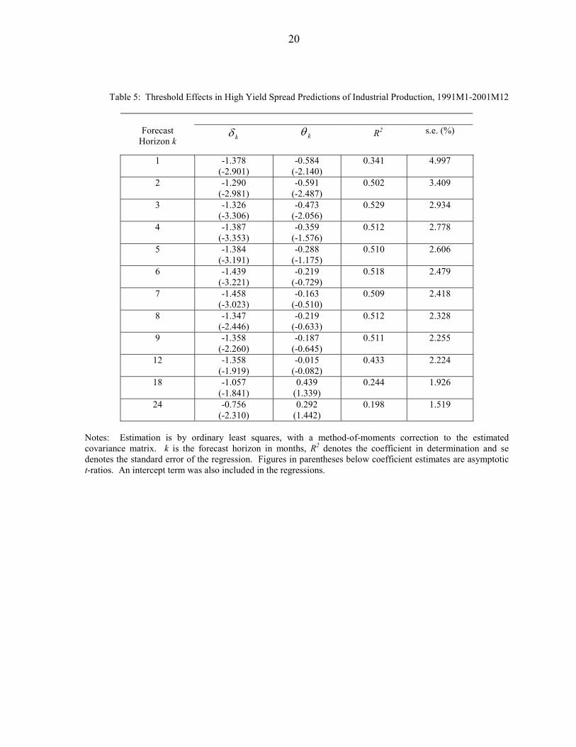
Table 3 shows the results of estimating the long-horizon term spread regressions for the most recent period, 1991M1-2001M12. Although the slope coefficients are significantly different from zero at the five percent level for horizons of up to two months, the t-ratios tail off after that so that none of them is significantly different from zero at the five percent level beyond the two-month horizon. The goodness of fit of the long-horizon regressions has also fallen dramatically at all horizons, relative to the corresponding levels for the 1970s and 1980s. Overall, therefore, the strong predictive content of the term spread with respect to future real economic activity seems to be largely confined to the period of the 1970s and 1980s. For the 1960s, the relationship appears to be much weakened, while for the 1990s the predictive power of the term spread appears to have virtually disappeared altogether. 4.2 High yield spread regressions Given that the market for below investment grade debt only developed in the US in the mid 1980s, lack of availability of data on the high yield spread forced us to consider only the most recent of the three sample periods, i.e. 1991M1-2001M12. The resulting long-horizon regressions are reported in Table 4. The sign of the estimated slope coefficient is negative every case: a larger spread predicts a slowdown, exactly as suggested by the theory of the financial accelerator. The predictive content of the high yield spread is quite striking. In every case, the estimated slope coefficient is strongly significantly different from zero at the one percent level, with t-ratios ranging in absolute value from around three to around nine. The goodness of fit, as measured by the coefficient of determination, is in nearly every case very much higher than the corresponding R2 for the term spread regressions, even during the “heyday” of the term spread during the 1970s and 1980s, the two exceptions being at the eighteen and twenty-four month horizons. Finally, since the theory of the financial accelerator suggests the possibility of non-linear interactions between financial variables and real activity, we examined whether “unusual” levels of high yield spreads convey additional information on real activity. Our proxy for “unusual” levels is a spread that is more than 1.5 standard deviations away from the sample mean. To test for this, we adjusted the long-horizon regression (7) to:

kttttkttkkktk RQIRQy ++ −+−+=∇ εθδγ )()( , (8) where It is a dummy variable that takes the value unity if the high yield spread is more than 1.5 standard deviations away from its mean over the sample period. The results of estimating this equation are shown in Table 5, and reveal that such abnormally high spreads do indeed predict an additional slowing down in growth, although only over the shorter horizons of up to three months.

9

5. Supply and demand innovations in real output Given the apparent importance of the high yield spread as a predictor of real economic activity during the last decade or so, we carried out some further investigations as to whether the spread is able to predict the cumulative growth in output when it is stripped of, alternately, its demand-side and supply-side components or, to be precise, its temporary and permanent components. Permanent and temporary output movements may be variously interpreted according to the underlying theoretical framework employed. In the traditional aggregate demand-aggregate supply (ADAS) model with a long-run vertical supply curve, for example, aggregate demand disturbances result in a temporary rise in output, while aggregate supply disturbances permanently affect the level of aggregate output. Blanchard and Quah (1989) use an ADAS framework in their analysis, and associate aggregate supply shocks with permanent shocks and aggregate demand shocks with temporary shocks. In this paper we shall follow their taxonomy. While it is possible that demand disturbances may have permanent effects on the real side of the economy, we concur with Blanchard and Quah that shocks having a permanent effect on output are likely to be due mostly if not wholly to supply-side factors, while those having only a temporary effect are likely to be due mostly if not wholly to demand-side factors. If the permanent long-run effects of demand disturbances are small relative to the long-run permanent effects of supply disturbances, then the Blanchard–Quah taxonomy is a useful organizing principle for empirical purposes. Readers rejecting this taxonomy, however, may simply reinterpret our analysis as investigating whether nominal spreads affect the permanent or the temporary components of real output movements. Given this taxonomy of permanent and temporary shocks to output, supply and demand shocks to real economic activity can be identified by imposing appropriate restrictions on the Wold representation of time series for real and nominal macroeconomic variables. In particular, consider the Wold representation for changes in the logarithm of output and the logarithm of prices:

=

∇∇

∑∞

= t

t

j jj

jjj

t

t Lpy

2

1

1 2221

1211

ςς

φφφφ

1

1 (9)

where the lmjφ are the parameters of the multivariate moving average representation and ς1t and ς2t are white noise innovations. We can identify ς1t and ς2t as demand and supply innovations in the following way. Write ςt =(ς1t ς2t )’, and denote the bivariate vector of innovations recovered from the vector autoregressive representation for )'( tt py 11 ∇∇ as υt Since the VAR representation is simply an inversion of the Wold representation (9), υt will in general be a linear function of ςt , υt =A ςt say, where A is a 2x2 matrix of constants. To

10

recover the underlying demand and supply innovations from the VAR residuals then requires that the four elements of A be identified, which requires four identifying restrictions. Three restrictions can be obtained by normalizing the variances of ς1t and ς2t to unity and setting their covariances to zero (see Blanchard and Quah, 1989, for a defense of these restrictions). The fourth, crucial identifying restriction, which effectively identifies ς1t as the demand innovation (or temporary output innovation), is the requirement that ς1t have no long-run effect on the (log-) level of real output, although it may affect the long-run price level. The latter restriction on the Wold representation (9) may be written:

∑∞

=

=1

11 0j

jφ . (10)

These four restrictions are then sufficient to recover the underlying temporary and permanent innovations to output, which, as we discussed above, may be interpreted as underlying demand and supply innovations respectively.4 Having identified the supply and demand innovations, we can then partition the moving average representation for real industrial output into counterfactual series, corresponding to the path that would have obtained in the absence of demand innovations and the path that would have obtained in the absence of supply innovations over the estimation period. We can then utilize these counterfactual series in tests of the predictive power of the high yield spread. We applied this method to the monthly series in the logarithm of industrial production and the consumer price index for the whole sample period, 1964M1-2001M12. Preliminary unit root (augmented Dickey–Fuller) tests on the data (not reported) showed the change in the logarithm of real industrial output, and the change in the logarithm of the consumer price index to be stationary processes. There was also no evidence of cointegration between industrial production and prices. This implies that output growth and inflation can be modeled as a bivariate moving average representation, which can be inverted to a pure autoregression not involving error correction terms. We therefore proceeded to estimate a vector autoregressive representation for the vector time series )'( 11 tt py ∇∇ . The order of the VAR was chosen by sequentially excluding the highest lags of both series, starting from a twelfth-order VAR, and testing the exclusion restrictions on the system using a likelihood ratio test. This process was stopped when the exclusion restrictions were jointly significant at the five percent level. This led to a choice of lag depth of six. The residuals from the estimated equations were judged to be approximately white noise, using either individual 4 For further details of the decomposition, see Blanchard and Quah (1989), Bayoumi and Taylor (1995) or Taylor (2002). Taylor (2002) discusses recursive restrictions of this type in the general multi-variable case.

11

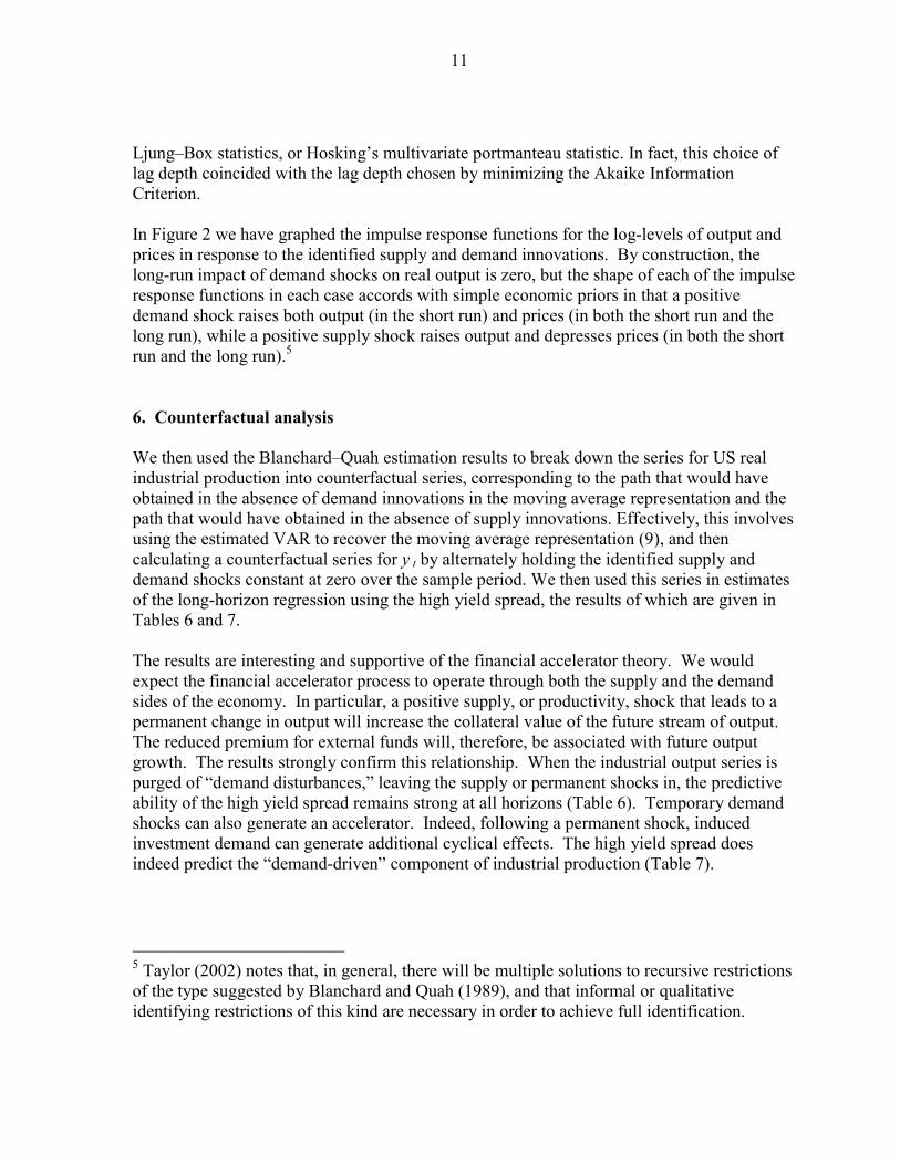
Ljung–Box statistics, or Hosking’s multivariate portmanteau statistic. In fact, this choice of lag depth coincided with the lag depth chosen by minimizing the Akaike Information Criterion. In Figure 2 we have graphed the impulse response functions for the log-levels of output and prices in response to the identified supply and demand innovations. By construction, the long-run impact of demand shocks on real output is zero, but the shape of each of the impulse response functions in each case accords with simple economic priors in that a positive demand shock raises both output (in the short run) and prices (in both the short run and the long run), while a positive supply shock raises output and depresses prices (in both the short run and the long run).5 6. Counterfactual analysis We then used the Blanchard–Quah estimation results to break down the series for US real industrial production into counterfactual series, corresponding to the path that would have obtained in the absence of demand innovations in the moving average representation and the path that would have obtained in the absence of supply innovations. Effectively, this involves using the estimated VAR to recover the moving average representation (9), and then calculating a counterfactual series for y t by alternately holding the identified supply and demand shocks constant at zero over the sample period. We then used this series in estimates of the long-horizon regression using the high yield spread, the results of which are given in Tables 6 and 7. The results are interesting and supportive of the financial accelerator theory. We would expect the financial accelerator process to operate through both the supply and the demand sides of the economy. In particular, a positive supply, or productivity, shock that leads to a permanent change in output will increase the collateral value of the future stream of output. The reduced premium for external funds will, therefore, be associated with future output growth. The results strongly confirm this relationship. When the industrial output series is purged of “demand disturbances,” leaving the supply or permanent shocks in, the predictive ability of the high yield spread remains strong at all horizons (Table 6). Temporary demand shocks can also generate an accelerator. Indeed, following a permanent shock, induced investment demand can generate additional cyclical effects. The high yield spread does indeed predict the “demand-driven” component of industrial production (Table 7). 5 Taylor (2002) notes that, in general, there will be multiple solutions to recursive restrictions of the type suggested by Blanchard and Quah (1989), and that informal or qualitative identifying restrictions of this kind are necessary in order to achieve full identification.

12

7. Conclusion Why did the term spread become a much weaker predictor of economic activity in the 1990s? Gertler and Lown (2000) suggest that changes in US monetary policy may have had something to do with this. In particular, a more robust defense of inflation starting in the mid-to-late 1980s may have changed private sector expectations with respect to future inflation. While the shift in monetary policy may have been influential, it is relevant that the predictive ability of the term spread was also weaker prior to 1970. The period during which the term spread was informative with respect to real activity—the 1970s and 1980s—was the period of the two oil shocks and characterized by high inflation (and possibly, therefore, greater inflation uncertainty) and volatile growth. We should expect in such a period that the negative covariance between current inflation and real activity would be most pronounced. A rise in current inflation, associated with a rise in short-term rates, would lead to a flattening of the term spread and lower real activity. However, in periods when inflation is low—and more predictable—these effects may be weaker.

In contrast, the financial accelerator creates a more robust foundation for the high yield spread as a predictor of future real macroeconomic activity. That relationship is based on financial frictions that amplify the business cycle. While such frictions, in particular, asymmetric information, may decline over time, that seems unlikely to occur in the immediate future. The robustness of this relationship is also suggested by the finding that the high yield spread captures both the supply-side (or permanent) shocks and the demand-side (temporary shocks).

13

Appendix: The negative covariation of inflation and output growth in a model with nominal wage inertia and long-run monetary neutrality

Consider the following simple, log-linear macroeconomic model, which displays long-run monetary neutrality and short-run nominal wage inertia induced through a wage formation equation in which wages are set in a two-period overlapping contracts framework:

ttt pmy −= (A1)

ttt ny θ+= (A2)

ttt wp θ−= (A3)

}*{| 2 nnEww ttt == − (A4) Equation (A1) represents the aggregate demand side of the economy as a function of real balances. The production function (A2) relates output to the level of employment, nt, and productivity θt. The price level is shown in (A3) to be a function of the nominal wage and productivity, while in (A4) the nominal wage contract is set two periods in advance at the level expected to generate full-employment level, n*. The model is closed by assuming that money and productivity are determined by the evolution of demand and supply shocks, edt and est respectively, as follows:

dttt emm += −1 (A5)

sttt e+= −1θθ . (A6) Assume that the covariance of edt and est is zero and that the supply and demand shocks have constant variances. Solving the model for inflation and output growth as a function of the exogenous demand and supply disturbances yields:

stdtt eep −=∇ −21 (A7)

stdtdtt eeey +−=∇ −21 , (A8) where 1∇ denotes the first-difference operator. Note that only supply shocks have a permanent effect on output, while both supply and demand shocks can affect long-run prices. Using (A7) and (A8), the covariance of growth and inflation is easily seen to be negative:

0)]()([),( 11 <+−=∇∇ stdttt eVareVarypCov . (A10)

14

References Bayoumi, Tamim, and Mark P. Taylor (1995). “Macroeconomic Shocks, the ERM, and Tri-Polarity.” Review of Economics and Statistics 77: 321–331. Bernanke, Ben S., and Mark Gertler (1995). “Inside the Black Box: The Credit Channel of Monetary Policy.” Journal of Economic Perspectives 9: 27-48. Bernanke, Ben S., and Mark Gertler (2001). “Should Central Banks Respond to Movements in Asset Prices?” American Economic Review 91: 253-57. Bernanke, Ben S., Mark Gertler, and Simon Gilchrist (1999). “The Financial Accelerator in a Quantitative Business Cycle Framework.” In John B. Taylor and Michael Woodford (Eds.) Handbook of Macroeconomics 1C.: 1341-93. Amsterdam; New York and Oxford: Elsevier Science, North-Holland. Bernard, Henri, and Stefan Gerlach (1998). “Does the Term Structure Predict Recessions? The International Evidence.” International Journal of Finance and Economics 3: 195-215. Blanchard, Olivier, and Danny Quah (1989). “The Dynamic Effects of Aggregate Demand and Supply Disturbances.” American Economic Review 79: 655–673. Caporale, Guglielmo M., (1994). “The Term Structure as a Predictor of Real Economic Activity: Some Empirical Evidence.” Discussion Paper DP-4-94, Centre for Economic Forecasting, London Business School. Chen, N. (1991). “Financial Investment Opportunities and the Real Economy.” Journal of Finance 46: 29–44. Chirinko, Robert S. (1993). “Business Fixed Investment Spending: Modeling Strategies, Empirical Results, and Policy Implications.” Journal of Economic Literature 31: 1875-1911. Deaton, Angus (1992). Understanding Consumption. Oxford: Clarendon Press. Dotsey, Michael (1998). “The Predictive Content of the Interest Rate Term Spread for Future Economic Growth.” Federal Reserve Bank of Richmond Economic Quarterly 84: 31-51. Estrella, Arturo, and Gikas A. Hardouvelis (1991). “The Term Structure as a Predictor of Real Economic Activity.” Journal of Finance 46: 555–576. Estrella, Arturo, and Frederic S. Mishkin (1998) “Predicting US Recessions: Financial Variables as Leading Indicators.” Review of Economics and Statistics 77: 321–331.

15

Estrella, Arturo, and Frederic S. Mishkin (1995b) “The Predictive Power of the Term Structure of Interest Rates in Europe and in the United States: Implications for the European Central Bank.” European Economic Review 41: 1375-1401. Fama, Eugene F. (1981). “Stock Returns, Real Activity, Inflation and Money.” American Economic Review 71: 545-565. Gertler, Mark, and Cara S. Lown (1999). “The Information in the High Yield Bond Spread for the Business Cycle: Evidence and Some Implications.” Oxford Review of Economic Policy 15: 132-150. Hansen, Lars P., (1982). “Large-Sample Properties of Generalized Method of Moments Estimators.” Econometrica 50: 1029–1054. Harvey, Campbell R., (1989). “Forecasts of Economic Growth from the Bond and Stock Markets.” Financial Analysts’ Journal September–October: 38–45. Hu, Z., (1993). “The Yield Curve and Real Activity.” International Monetary Fund Working Paper 93/19, Washington D.C. Laurent, Robert (1988). “An Interest Rate Based Indicator of Monetary Policy.” Federal Reserve Bank of Chicago Economic Perspectives 12: 3-14. Peel, David A., and Mark P. Taylor (1998) “The Slope of the Yield Curve and Real Economic Activity: Tracing the Transmission Mechanism.” Economics Letters 59:353-360. Plosser, Charles I., and K.Geert Rouwenhurst (1994). “International Term structures and Real Economic Growth.” Journal of Monetary Economics 33: 133–155. Stock, James H., and Mark Watson (1989). “New Indexes of Coincident and Leading Indicators.” In: Olivier J. Blanchard and Stanley S. Fischer (Eds.) NBER Macroeconomics Annual 1989. Cambridge MA: MIT Press Taylor, Mark P. (1992). “Modeling the Yield Curve.” Economic Journal 102: 524-37.

Taylor, Mark P. (1999). “Real Interest Rates and Macroeconomic Activity.” Oxford Review of Economic Policy 15: 95-113. Taylor, Mark P. (2002). “Estimating Structural Macroeconomic Shocks Through Long-Run Recursive Restrictions on Vector Autoregressive Models: The Problem of Identification.” Mimeo, Department of Economics, University of Warwick.

16

Table 1: Term Spread Predictions of Industrial Production Growth, 1971M1-1990M12

Forecast

Horizon k kβ R2 s.e. (%)

1 2.038 (4.080)

0.071 10.433

2 2.255 (3.566)

0.120 8.610

3. 2.392 (3.625)

0.165 7.612

4 2.449 (3.734)

0.200 6.931

5 2.438 (3.833)

0.223 6.435

6 2.409 (3.870)

0.243 6.005

7 2.395 (3.954)

0.269 5.586

8 2.391 (3.938)

0.294 5.243

9 2.370 (3.868)

0.316 4.931

12 2.349 (3.928)

0.384 4.223

18 2.102 (3.864)

0.445 3.353

24 1.632 (4.565)

0.375 3.029

Notes: Estimation is by ordinary least squares, with a method-of-moments correction to the estimated covariance matrix. k is the forecast horizon in months, R2 denotes the coefficient in determination and se denotes the standard error of the regression. Figures in parentheses below coefficient estimates are asymptotic t-ratios. An intercept term was also included in the regressions.

17

Table 2: Term Spread Predictions of Industrial Production Growth, 1964M1-1970M12

Forecast

Horizon k kβ R2 s.e. (%)

1 1.366 (0.428)

0.003 9.790

2 1.798 (0.536)

0.010 7.272

3. 2.703 (0.709)

0.028 6.263

4 3.934 (1.027)

0.068 5.652

5 5.059 (1.470)

0.119 5.245

6 6.018 (2.127)

0.182 4.812

7 6.898 (2.912)

0.252 4.403

8 7.513 (2.893)

0.310 4.125

9 8.070 (2.414)

0.372 3.821

12 7.424 (1.996)

0.365 3.593

18 5.303 (1.947)

0.284 2.980

24 3.400 (1.530)

0.175 2.614

Notes: Estimation is by ordinary least squares, with a method-of-moments correction to the estimated covariance matrix. k is the forecast horizon in months, R2 denotes the coefficient in determination and se denotes the standard error of the regression. Figures in parentheses below coefficient estimates are asymptotic t-ratios. An intercept term was also included in the regressions.

18

Table 3: Term Spread Predictions of Industrial Production Growth, 1991M1-2001M12

Forecast Horizon k

kβ R2 s.e. (%)

1 0.880 (1.981)

0.025 6.082

2 1.015 (2.031)

0.052 4.812

3. 1.085 (1.888)

0.069 4.423

4 1.116 (1.729)

0.079 4.212

5 1.129 (1.595)

0.090 3.980

6 1.164 (1.520)

0.104 3.789

7 1.216 (1.497)

0.124 3.610

8 1.269 (1.479)

0.145 3.438

9 1.275 (1.450)

0.158 3.285

12 1.174 (1.416)

0.155 3.021

18 0.870 (1.538)

0.122 2.484

24 0.908 (1.696)

0.170 2.148

Notes: Estimation is by ordinary least squares, with a method-of-moments correction to the estimated covariance matrix. k is the forecast horizon in months, R2 denotes the coefficient in determination and se denotes the standard error of the regression. Figures in parentheses below coefficient estimates are asymptotic t-ratios. An intercept term was also included in the regressions.

19

Table 4: High Yield Spread Predictions of Industrial Production Growth, 1991M1-2001M12

Forecast

Horizon k kδ R2 s.e. (%)

1 -2.092 (-9.195)

0.326 5.056

2 -2.030 (-8.355)

0.495 3.512

3. -1.998 (-6.813)

0.562 3.031

4 -1.951 (-5.482)

0.573 2.866

5 -1.852 (-4.820)

0.570 2.734

6 -1.771 (-4.375)

0.560 2.654

7 -1.686 (-3.994)

0.540 2.614

8 -1.617 (-3.739)

0.532 2.544

9 -1.555 (-3.543)

0.523 2.472

12 1.406 (-3.428)

0.489 2.348

18 -1.009 (-3.974)

0.342 2.150

24 -0.784 (-2.934)

0.254 2.035

Notes: Estimation is by ordinary least squares, with a method-of-moments correction to the estimated covariance matrix. k is the forecast horizon in months, R2 denotes the coefficient in determination and se denotes the standard error of the regression. Figures in parentheses below coefficient estimates are asymptotic t-ratios. An intercept term was also included in the regressions.

20

Table 5: Threshold Effects in High Yield Spread Predictions of Industrial Production, 1991M1-2001M12

Forecast

Horizon k kδ kθ R2 s.e. (%)

1 -1.378 (-2.901)

-0.584 (-2.140)

0.341 4.997

2 -1.290 (-2.981)

-0.591 (-2.487)

0.502 3.409

3 -1.326 (-3.306)

-0.473 (-2.056)

0.529 2.934

4 -1.387 (-3.353)

-0.359 (-1.576)

0.512 2.778

5 -1.384 (-3.191)

-0.288 (-1.175)

0.510 2.606

6 -1.439 (-3.221)

-0.219 (-0.729)

0.518 2.479

7 -1.458 (-3.023)

-0.163 (-0.510)

0.509 2.418

8 -1.347 (-2.446)

-0.219 (-0.633)

0.512 2.328

9 -1.358 (-2.260)

-0.187 (-0.645)

0.511 2.255

12 -1.358 (-1.919)

-0.015 (-0.082)

0.433 2.224

18 -1.057 (-1.841)

0.439 (1.339)

0.244 1.926

24 -0.756 (-2.310)

0.292 (1.442)

0.198 1.519

Notes: Estimation is by ordinary least squares, with a method-of-moments correction to the estimated covariance matrix. k is the forecast horizon in months, R2 denotes the coefficient in determination and se denotes the standard error of the regression. Figures in parentheses below coefficient estimates are asymptotic t-ratios. An intercept term was also included in the regressions.

21

Table 6: High Yield Spread Predictions of Industrial Production Growth with Industrial Production Purged of Demand-Side Disturbances, 1991M1-2001M12

Forecast

Horizon k kδ R2 s.e. (%)

1 -0.392 (-2.366)

0.070 2.173

2 -0.474 (-1.923)

0.126 1.956

3. -0.571 (-1.799)

0.182 1.935

4 -0.637 (-1.851)

0.222 1.924

5 -0.687 (-2.026)

0.254 1.864

6 -0.714 (-2.142)

0.271 1.811

7 -0.721 (-2.213)

0.277 1.782

8 -0.730 (-2.293)

0.285 1.767

9 -0.731 (-2.400)

0.294 1.732

12 -0.730 (-2.700)

0.311 1.672

18 -0.679 (-3.966)

0.314 1.567

24 -0.592 (-2.330)

0.229 1.700

Notes: Estimation is by ordinary least squares, with a method-of-moments correction to the estimated covariance matrix. The series for industrial production has been purged of demand-side disturbances using the Blanchard-Quah method described in the text. k is the forecast horizon in months, R2 denotes the coefficient in determination and se denotes the standard error of the regression. Figures in parentheses below coefficient estimates are asymptotic t-ratios. An intercept term was also included in the regressions.

22

Table 7: High Yield Spread Predictions of Industrial Production Growth with Industrial Production Purged of Supply-Side Disturbances, 1991M1-2001M12

Forecast

Horizon k kδ R2 s.e. (%)

1 -1.785 (-6.189)

0.212 5.255

2 -1.684 (-5.009)

0.337 3.701

3. -1.622 (-4.141)

0.398 3.186

4 -1.534 (-3.620)

0.411 2.960

5 -1.407 (-3.282)

0.387 2.800

6 -1.292 (-3.155)

0.356 2.685

7 -1.168 (-3.167)

0.323 2.589

8 -1.078 (-3.171)

0.310 2.461

9 -0.998 (-3.183)

0.302 2.320

12 -0.858 (-2.994)

0.284 2.094

18 -0.635 (-2.758)

0.221 1.862

24 -0.482 (-1.904)

0.142 1.856

Notes: Estimation is by ordinary least squares, with a method-of-moments correction to the estimated covariance matrix. The series for industrial production has been purged of supply-side disturbances using the Blanchard-Quah method described in the text. k is the forecast horizon in months, R2 denotes the coefficient in determination and se denotes the standard error of the regression. Figures in parentheses below coefficient estimates are asymptotic t-ratios. An intercept term was also included in the regressions.

Figu

re 1

: U

S In

flatio

n an

d O

utpu

t Gro

wth

, 195

8-20

01

-25

-20

-15

-10-50510152025 19

58M

119

62M

119

66M

119

70M

119

74M

119

78M

119

82M

119

86M

119

90M

119

94M

119

98M

120

02M

1

12-m

onth

infla

tion

rate

12-m

onth

gro

wth

in o

utpu

t

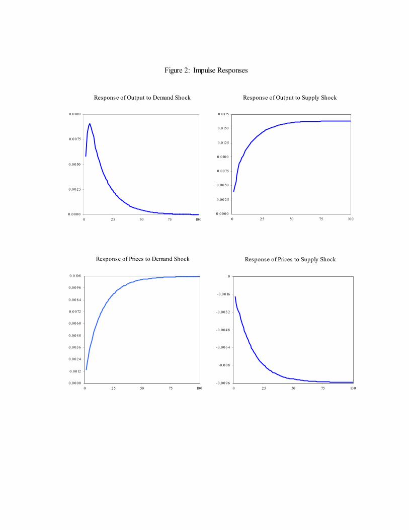
Figure 2: Impulse Responses

Response of Output to Demand Shock

0.0000

0 .0 025

0 .0 050

0 .00 75

0 .0100

0 25 50 75 10 0

Response of Output to Supply Shock

0 .0 000

0 .00 25

0 .00 50

0 .0075

0 .0100

0 .0125

0 .0150

0 .0175

0 25 50 75 100

Response of Prices to Demand Shock

0 .0 000

0 .00 12

0 .0 024

0 .0 036

0 .0 048

0 .0 060

0 .00 72

0 .0 084

0 .0 096

0 .0108

0 25 50 75 100

Response of Prices to Supply Shock

-0 .009 6

-0 .00 8

-0 .006 4

-0 .004 8

-0 .003 2

-0 .0 016

0

0 25 50 75 100