Institutions Rule - Harvard Kennedy School - Harvard University
Upload
truongkietCategory
view
215download
0
The Harvard CollegeMathematics Review
Volume 3 Spring 2011
In this issue:
CHRISTOPHER POLICASTROArtin's Conjecture
ZHAO CHEN, KEVIN DONAGHUE& ALEXANDER ISAKOV
A Novel Dual-Layered Approach to Geographic Profiling in Serial Crimes
MICHAEL J. HOPKINSThe Three-Legged Theorem
MLRA Student Publication of Harvard College

Website. Further information about The HCMR can befound online at the journal's website,
h t t p : / /www. thehcmr.o rg / fl )
Instructions for Authors. All submissions should include the name(s) of the author(s), institutional affiliations (ifany), and both postal and e-mail addresses at which the corresponding author may be reached. General questions shouldbe addressed to Editor-in-Chief Rediet Abebe at hcmr@ hcs .harvard.edu.
Articles. The Harvard College Mathematics Review invitesthe submission of quality expository articles from undergraduate students. Articles may highlight any topic in undergraduate mathematics or in related fields, including computer science, physics, applied mathematics, statistics, and mathematical economics.
Authors may submit articles electronically, in .pdf, .ps,or .dvi format, to [email protected], or in hardcopy to
The Harvard College Mathematics ReviewStudent Organization Center at HillesBox # 36059 Shepard StreetCambridge, MA 02138.
Sponsorship. Sponsoring The HCMR supports the undergraduate mathematics community and provides valuablehigh-level education to undergraduates in the field. Sponsorswill be listed in the print edition of The HCMR and on a special page on the The HCMR's website, (1). Sponsorship isavailable at the following levels:
Sponsor $0 - $99Fellow $100-$249Friend $250 - $499
Contributor $500-$1,999Donor $2,000 - $4,999Patron $5,000 - $9,999
Benefactor $10,000 +
Contributors ■ Jane Street Capital • The Harvard University Mathematics DepartmentCover Image. The image on the cover depicts severalfunctions, whose common zero locus describes an algebraicvariety (which is in this case an elliptic curve). This issue'sarticle "Hilberts Nullstellensatz and Schemes" by Miles Edwards (p. 17) describes one of the foundational theorems inalgebraic geometry, relating an ideal in a polynomial ring toits corresponding algebraic variety. This image was created inAsymptote by Graphic Artists Eric Larson and KatherineBanks.
Submissions should include an abstract and reference list. Figures, if used, must be of publication quality. If a paper isaccepted, high-resolution scans of hand drawn figures and/orscalable digital images (in a format such as eps) will be required.
Problems. The HCMR welcomes submissions of originalproblems in all mathematical fields, as well as solutions topreviously proposed problems.
Proposers should send problem submissions to ProblemsEditor Lucia Mocz at hemr-problems@hcs. harvard,edu or to the address above. A complete solution or a detailedsketch of the solution should be included, if known.
Solutions should be sent to hcmr-solutions@hcs .harvard.edu or to the address above. Solutions shouldinclude the problem reference number. All correct solutionswill be acknowledged in future issues, and the most outstanding solutions received will be published.
Advertising. Print, online, and classified advertisementsare available; detailed information regarding rates can befound on The HCMR's website, (1). Advertising inquiriesshould be directed to hemr- advert ise@hcs .harvard,edu, addressed to Business Manager Gerishom Gimaiyo.
Subscriptions. One-year (two issue) subscriptions areavailable, at rates of $5.00 for students, $7.50 for other individuals, and $15.00 for institutions. Subscribers should mailchecks for the appropriate amount to The HCMR's postal address; confirmation e-mails or queries should be directed [email protected].
©2007-2011 The Harvard College Mathematics ReviewHarvard College
Cambridge, MA 02138
The Harvard College Mathematics Review is produced andedited by a student organization of Harvard College.
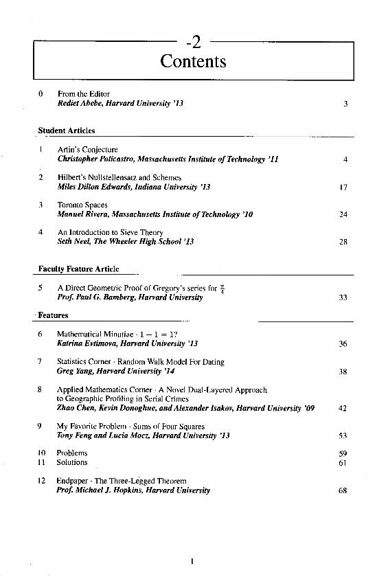
— -2 —Contents
0 From the EditorRediet Abebe, Harvard University '13
Student Articles
Artin's ConjectureChristopher Policastro, Massachusetts Institute of Technology '11 4
Hilbert's Nullstellensatz and SchemesM i l e s D i l l o n E d w a r d s , I n d i a n a U n i v e r s i t y ' 1 3 1 7
Toronto SpacesManuel Rivera, Massachuset ts Inst i tu te of Technology '10 24
An Introduction to Sieve TheoryS e t h N e e l , T h e W h e e l e r H i g h S c h o o l ' 1 3 2 8
Faculty Feature Article
5 A Direct Geometric Proof of Gregory's series for \P r o f . P a u l G . B a m b e r g , H a r v a r d U n i v e r s i t y 3 3
Features
6 Mathematical Minutiae -1 + 1 = 1?K a t r i n a E v t i m o v a , H a r v a r d U n i v e r s i t y ' 1 3 3 6
7 Statistics Corner • Random Walk Model For DatingG r e g Y a n g , H a r v a r d U n i v e r s i t y ' 1 4 3 8
8 Applied Mathematics Corner • A Novel Dual-Layered Approachto Geographic Profiling in Serial CrimesZhao Chen, Kevin Donoghue, and Alexander Isakov, Harvard University '09 42
9 My Favorite Problem • Sums of Four SquaresTo n y F e n g a n d L u c i a M o c z , H a r v a r d U n i v e r s i t y ' 1 3 5 3
1 0 P r o b l e m s 5 91 1 S o l u t i o n s 6 1
12 Endpaper • The Three-Legged TheoremP r o f . M i c h a e l J . H o p k i n s , H a r v a r d U n i v e r s i t y 6 8

Editor-in-ChiefRediet Abebe'13
Business ManagerGerishom Gimaiyo '13
A r t i c l e s E d i t o r A s s o c i a t e D i r e c t o rF r a n c o i s G r e e r ' 1 1 E r i c L a r s o n ' 1 3F e a t u r e s E d i t o r A s s i s t a n t A r t i c l e s E d i t o rK a t h e r i n e B a n k s ' 1 2 A k h i l M a t h e w ' 1 4P r o b l e m s E d i t o r A s s i s t a n t P r o b l e m s E d i t o r sL u c i a M o c z ' 1 3 G e Ya n g ' 1 4 a n d L e v e n t A l p o g e ' 1 4
Issue Production DirectorsEric Larson '13 and Katherine Banks '12
Graphic ArtistsEric Larson '13 and Katherine Banks' 12
Editors EmeritusZachary Abel' 10, Scott Kominers '09/AM' 10/PhD' 11, Ernest Fontes ' 10
WebmasterRediet Abebe'13
B o a r d o f R e v i e w e r s B o a r d o f C o p y E d i t o r sL e v e n t A l p o g e ' 1 4 R e d i e t A b e b e ' 1 3A n i r u d h a B a l a s u b r a m a n i a n ' 1 4 J o h n C a s a l e ' 1 2K a t h e r i n e B a n k s ' 1 2 A s h o k C u t k o s k y ' 1 3J o h n C a s a l e ' 1 2 Y a l e F a n ' 1 4A s h o k C u t k o s k y ' 1 3 F r a n c o i s G r e e r ' 1 1Y a l e F a n ' 1 4 E r i c L a r s o n ' 1 3F r a n c o i s G r e e r ' 1 1 G e f f o r y L e e ' 1 4E r i c L a r s o n ' 1 3 A k h i l M a t h e w ' 1 4G e o f f r e y L e e ' 1 4 L u c i a M o c z ' 1 3A k h i l M a t h e w ' 1 4 Z a c h a r y Y o u n g ' 1 4Lucia Mocz'13Ge Yang'14Zachary Young '14
Faculty AdviserProfessor Peter Kronheimer, Harvard University

oFrom the Editor
Rediet AbebeHarvard University '13Cambridge, MA 02138
r tes faye@co l lege .harvard .edu
When I took on the role of Editor-in-Chief of the Harvard College Math Review in May 2010,1was not sure how HCMR was going to turn out, or if we were even going to have an HCMR by theend of the school year. After more than a year of inactivity, HCMR was potentially faced with major changes and decisions. It was not until we recruited new staff and executive board members thatI became fully confident that, once again, we were going to have an issue that would help studentslearn and appreciate advanced mathematics like the founder and former Editors had envisioned itwould.
Since September when we started accepting applications for the different position until a fewweeks ago when we were making final edits on the articles, members of the HCMR executive boardand the staff have worked tirelessly to make this issue one of the strongest ones we have had. Tothis end, I would like to thank the Articles Editor, Francois Greer, the Features Editor, KatherineBanks, the Problems Editor, Lucia Mocz and their staff for all the hard work. I would also like tothank Eric Larson for taking up several roles and working on each flawlessly.
The executive board is thankful for Professor Peter Kronheimer, the Harvard UniversityMathematics Department and the staff at the Student Organization Center at Hilles for theircontinual advice and support. You continue to make the HCMR a success and we are glad to haveyour support year after year.
We also thank the HCMR advisors and sponsors, whose generous contributions have been afoundation for the journal's success.
I would also like to personally express my deepest gratitude to Editor Emeriti Zach Abel, ScottD. Kominers and Ernest E. Fontes for constantly being there to answer all the major and minorquestions I had even after their graduation from Harvard College. Your invaluable expertise andguidance has inspired the entire staff.
Finally, the executive board would like to thank all our writers and readers in the United Statesand around the world. We are honored at all the feedback and contributions we have received sofar. As always, please direct your comments, questions and submissions to [email protected] the board is in the process of discussing potential changes in the structure, web and print output,your feedback is more valuable than ever. For updates, check www.thehcmr.org/
Rediet AbebeEditor-in-Chief, The HCMR

STUDENT ARTICLE1
Artin's Conjecture
Christopher Policastro*Massachusetts Institute of Technology ' 11
Cambridge, MA 02138cpol i@mit .edu
AbstractWe survey Artin L-functions by providing the necessary background to describe Artin's conjecture.Having detailed the basic properties of Artin L-series, we show that they extend meromorphicallyto the plane, and discuss recent research on this continuation. We assume the reader has someknowledge of group representations, algebraic number theory, and complex analysis.
1.1 IntroductionCertain arithmetic properties of a number field are contained within holomorphic functions calledL-series. These series are defined in some right half-plane and can be meromorphically continuedto C. The resulting L-functions share several analytic properties that can be used to characterizethem.
The L-series for a number field take two rather different forms that can be reconciled in somecases. The abelian type were introduced by Erich Hecke, who constructed them from characters ofray class groups in an attempt to generalize the Dirichlet L-series
* > x ) = Z * & ( i . Dn > l
where \ : (Z/raZ)* -+ C* is a homomorphism for some ra. The nonabelian type owe to EmilArtin, who defined them by representations of Galois groups following the work of Takagi. Someyears after he described the basic properties of these L-series, Richard Brauer proved that theyadmit a meromorphic continuation to the plane.
Artin famously conjectured that with few exceptions this continuation was holomorphic. Thoughprogress continues to be made on the conjecture, it remains one of the most important outstandingproblems in mathematics. The goal of this paper is to attract readers to this very active branch ofanalytic number theory.
The rest of the paper is as follows. Having recalled several facts about representations of finite groups and Hecke L-functions, we define incomplete Artin L-series and prove their functorialproperties. Having shown that these series meromorphically extend to C, we verify Artin's conjecture for a class of extensions, and briefly discuss works of Langlands and Selberg as they apply tothe conjecture.
Before continuing let us fix some notation. Throughout we have k denote a number field,that is, a finite extension of Q. Let Ok be the ring of integers, and for an ideal o in Ofc, let91(a) = Card(Ojt/a). For K/k a finite extension, and ^J|p primes, we let ff and ef denotethe residual degree and ramification index. By a place v of k, we mean an equivalence class ofnontrivial valuations of k. These are of three sorts: finite places corresponding to primes of k, realplaces corresponding to the real embeddings of A:, and complex places corresponding to the pairsof conjugate complex embeddings of k.
t Christopher Policastro is a senior studying mathematics at the Massachusetts Institute of Technology. Hismathematical interests lie somewhere between geometry and algebra. At the moment, he is leaning towardsrepresentation theory.
C h r i s t o p h e r P o l i c a s t r o — A r t i n ' s C o n j e c t u r e 5
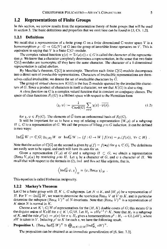
1.2 Representations of Finite GroupsIn this section, we review results from the representation theory of finite groups that will be usedin section 3. The basic definitions and properties that we omit here can be found in [3, Ch. 1,2].
1.2.1 DefinitionsWe recall that a representation of a finite group G on a finite dimensional C-vector space V is ahomomorphism p : G -> GL(V") of G into the group of invertible linear operators on V. This isequivalent to saying that V is a finite C[G]-module.
The complex valued function \(s) = Tr(p(s)) s e G is called the character of the representation p. We know that a character completely determines a representation, in the sense that two finiteC[G]-modules are isomorphic iff they have the same character. The character of a 1-dimensionalrepresentation is called abelian.
By Maschke's theorem, C[G] is semisimple. Therefore each finite C[G]-module decomposesinto a direct sum of irreducible representations. Characters of irreducible representations are themselves called irreducible; we denote the set of irreducible characters by G.
The group of virtual characters K(G) is the free Z-module spanned by the irreducible characters of G. Since a product of characters is itself a character, we see that K(G) is also a ring.
A class function on G is a complex valued function that is constant on conjugacy classes. Thespace of class functions Fc(G) is a Hilbert space with respect to the Hermitian form
<*'*>:=cdb^5*«-*w- (L2)for x, ip € Fc(G). The elements of G form an orthonormal basis of Fc(G).It will be important for us to have a way of relating a representation (W, p) of a subgroup
H C G to a representation of G. We call the process of lifting p to G induction. It can be definedin two ways:
Indg W := C[G] ®C[H] W or Indg W := {/ : G -> W \ f(rs) = pT(f(s)), Vr G H} .
Note that the action of C[G] on the second is given by g(f) = /(•#) forg e C[G]. The definitionsare easily seen to be equal, and each will have its uses for us.
Given a representation (V,p) of G and a subgroup H c G, we obtain a representation(Resn V,p\h) by restricting p to H. Let \ be a character of G, and ip a character of H. Werecall that with respect to the formula in (2), Ind and Res act like adjoints, that is,
(lnd% ip,x) = (^,ResHx)H
This equation is called Frobenius reciprocity.
1.2.2 Mackey's TheoremLet G be a finite group with H, K C G subgroups. Let N < K, and (W, p) be a representation ofH. For V =: Indg W, we want to determine the restriction Res^ V of V to K, and in particulardetermine the subspace (Res*: V)N of iV-invariants. Note that (Res^ V)N is a representation ofif since iV is normal in K.
Choose a set K \ G/H of representatives for the (H, K) double cosets of G; this means G isthe disjoint union of KsH for s e K \ G/H. Let Hs = sHs~x n K. Note that Hs is a subgroupof K, and the rule ps(#) := p(x) for a: e #s gives a homomorphism ps : Hs -+ GL(sW), wheresW is taken in V. Inducing ps to K for each s, we have the following result.Proposition 1. (Res* Indg W)N =i ©s€/AG/H(Indgs sW)N.
The proposition can be obtained as an immediate generalization of [6, Sec. 7.3].
6 T h e H a r v a r d C o l l e g e M a t h e m a t i c s R e v i e w 3
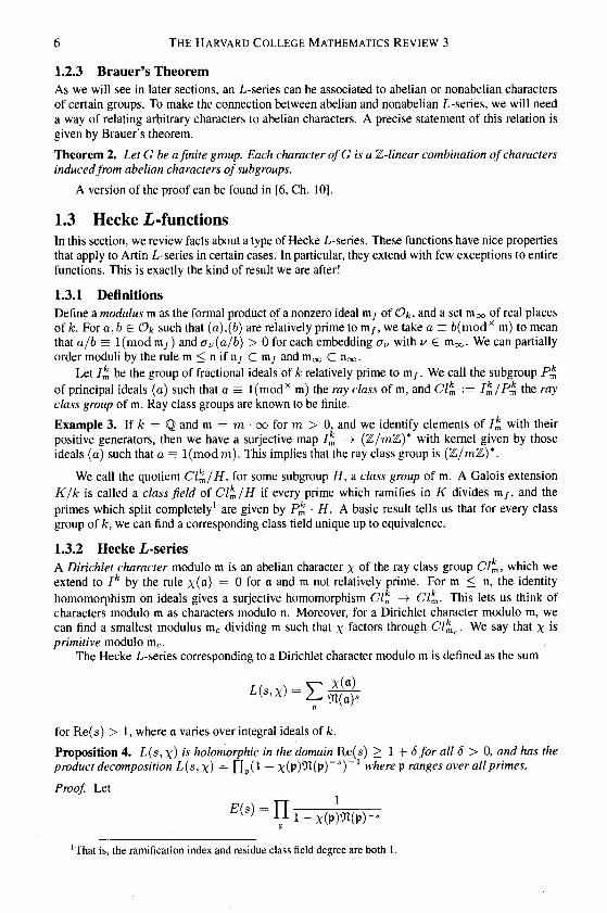
1.2.3 Brauer's TheoremAs we will see in later sections, an L-series can be associated to abelian or nonabelian charactersof certain groups. To make the connection between abelian and nonabelian L-series, we will needa way of relating arbitrary characters to abelian characters. A precise statement of this relation isgiven by Brauer's theorem.Theorem 2. Let G be a finite group. Each character ofG is a Z-linear combination of charactersinduced from abelian characters of subgroups.
A version of the proof can be found in [6, Ch. 10].
1.3 Hecke L-functionsIn this section, we review facts about a type of Hecke L-series. These functions have nice propertiesthat apply to Artin L-series in certain cases. In particular, they extend with few exceptions to entirefunctions. This is exactly the kind of result we are after!
1.3.1 DefinitionsDefine a modulus m as the formal product of a nonzero ideal m/ of Ok, and a set rrioo of real placesof k. For a,b e Ok such that (a),(b) are relatively prime to m/, we take a = b(modx m) to meanthat a/b = l(modm/) and a„(a/b) > 0 for each embedding au with v G moo. We can partiallyorder moduli by the rule m < n if n/ C m/ and m^ C noo.
Let I* be the group of fractional ideals of k relatively prime to m/. We call the subgroup P*of principal ideals (a) such that a = l(modx m) the ray class of m, and C/m := Im/Pm the rayclass group of m. Ray class groups are known to be finite.Example 3. If k — Q and m = ra • oo for ra > 0, and we identify elements of /£ with theirpositive generators, then we have a surjective map /£ -> (2/mZ)* with kernel given by thoseideals (a) such that a = l(modra). This implies that the ray class group is (Z/raZ)*.
We call the quotient Cl^/H, for some subgroup H, a class group of m. A Galois extensionK/k is called a class field of Cl^/H if every prime which ramifies in K divides m/, and theprimes which split completely1 are given by P^ • H. A basic result tells us that for every classgroup of k, we can find a corresponding class field unique up to equivalence.1.3.2 Hecke i>-seriesA Dirichlet character modulo m is an abelian character \ of the ray class group C/f^, which weextend to Ik by the rule x(a) = 0 for a and m not relatively prime. For m < n, the identityhomomorphism on ideals gives a surjective homomorphism C/„ -+ Cl1^. This lets us think ofcharacters modulo m as characters modulo n. Moreover, for a Dirichlet character modulo m, wecan find a smallest modulus mc dividing m such that \ factors through Cl^c. We say that \ isprimitive modulo mc.
The Hecke L-series corresponding to a Dirichlet character modulo m is defined as the sum
L(s,X) = Yl X(a)W(a)s
for Re(s) > 1, where a varies over integral ideals of k.Proposition 4. L(s, x) is holomorphic in the domain Re(s) > 1 + 6 for all 8 > 0, and has theproduct decomposition L(s,x) = Ylp(l ~ x(p)^(p)~s)_1 where p ranges over all primes.Proof. Let
■ x ( p W p ) -
!That is, the ramification index and residue class field degree are both 1.

Christopher Policastro—Artin's Conjecture
for Re(s) > 1 + 8 and p such that x(p) ¥" 0- Formally taking the logarithm gives
. x(P)n1
P n > \p n > \ V r /
Since x is abelian, and C7* is finite, we have \x(p)\ = 1. As |91(p)s| = 9t(p)Re(s) > pf*(1+6) >p1+6, and at most [k : Q] primes lie above p, we have that
p n > l v r / p n > l ^
This bound does not depend on s. So we see that log E(s) converges absolutely and uniformly forRe(s) > 1 4- S. Theref6re E(s) is holomorphic in this half plane, and we are left showing thatE(s) = L(s,X).
Expand the factors in E(s) corresponding to the finitely many primes pi... pr such thatW(pi) < N, and multiply them. This yields
l l l - x f a W P i ) - l l A K ( P i ) s J ^ < l i ( * Y L , O T ( a ) » u }t = l A v r t / v r t / 1 = 1 x v r i / ' m ( a ) < N V ' m ( a ) > N V '
where the prime indicates that the second sum in the last equality is only over integral ideals a thatare divisible only by the primes pi... pr. By (4) we have
r 1 1
Ui-x(Pin(Pi)-s~L{s'x) -„?..wS« n ( o ) > N v ;i = l
so we need to show that this last term tends to zero as N —> oo to complete the proof. Now
1 ' 1 1
where the second sum is over integral ideals only divisible by pi... pr. So using the bound in (3)for the case of x trivial and s = 1 + S, we see that Yl<y\(a)<N 9t(a)-1-(5 is monotone increasingand bounded above by C(l 4- £)[fc:Q] as N -+ oo. Hence the tail J2m(a)>N ^(a)-1-5 convergest o z e r o a s N — > o o . D
From Example 3, we see that Hecke L-series do indeed generalize Dirichlet L-series. Thoughit requires some work, we can extend Hecke L-series to the plane in much the same way we extendDirichlet L-series. We obtain the following result, due to Hecke.Proposition 5. L(s, x) can be holomorphic ally continued to Cfor \ nontrivial. For x trivial, itextends to a meromorphic function with poles at s = 0,1.
For a proof of this fact see [5, VII.8].
1.4 Artin L-functionsWe are at last ready to describe Artin L-series. Since (1) is the Riemann zeta function for ra = 1,the series L(s, Xtriv) for m = Ok has historically been denoted as Qk(s). When Artin introduceda L-series in [1] attached to nonabelian characters, he hoped to verify a conjecture of Dedekindconcerning the poles of C/r.W/C* (s) for K/k a Galois extension.
Assuming that K/k is a class field, Weber had shown that Ck(s)/0c(s) could be decomposedinto a product of L-series for nontrivial characters of the corresponding class group. By Hecke's
8 T h e H a r v a r d C o l l e g e M a t h e m a t i c s R e v i e w 3
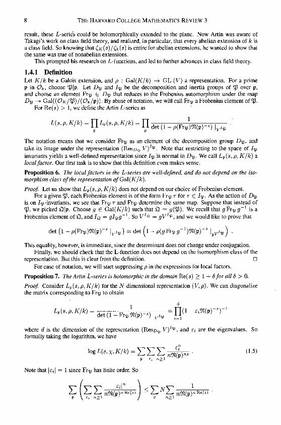
result, these L-serie's could be holomorphically extended to the plane. Now Artin was aware ofTakagi's work on class field theory, and realized, in particular, that every abelian extension of k isa class field. So knowing that Oc(s)/Cfc(s) is entire for abelian extensions, he wanted to show thatthe same was true of nonabelian extensions.
This prompted his research on L-functions, and led to further advances in class field theory.
1.4.1 DefinitionLet K/k be a Galois extension, and p : Gai(K/k) -+ GL (V) a representation. For a primep in Ok, choose ^3|p. Let Dy and Lp be the decomposition and inertia groups of <P over p,and choose an element Fr j G D<# that reduces to the Frobenius automorphism under the mapD<# r-» Gal((OK/^)/(Ok/p))- By abuse of notation, we will call Fr*p a Frobenius element of <$.
For Re(s) > 1, we define the Artin L-series as
u „ f , K m - n m » » m - n J e , ( 1 _ P ( R ^ ( > ) - , , l v , v ■
The notation means that we consider Fr.^ as an element of the decomposition group Dy, andtake its image under the representation (Resz^ V)1^. Note that restricting to the space of Lpinvariants yields a well-defined representation since L# is normal in D<#. We call Lp(s, p, K/k) alocal factor. Our first task is to show that this definition even makes sense.Proposition 6. The local factors in the L-series are well-defined, and do not depend on the isomorphism class of the representation ofGd\(K/k).Proof Let us show that Lp (s, p, K/k) does not depend on our choice of Frobenius element.
For a given *J3, each Frobenius element is of the form Fr r for r G I<#. As the action of D<#is on I<#-invariants, we see that Fr<p r and Fr># determine the same map. Suppose that instead of<P, we picked Q\p. Choose g G Ga\(K/k) such that Q = g(ty). We recall that gFr^g'1 is aFrobenius element of £3, and Iq = gl<#g~l. So VIq = gVLv, and we would like to prove that
det(l-p(Fr^)01(p)-s \viv)=det(l-p(gFrvg-1)yi(p)-s |^) .This equality, however, is immediate, since the determinant does not change under conjugation.
Finally, we should check that the L-function does not depend on the isomorphism class of ther e p r e s e n t a t i o n . B u t t h i s i s c l e a r f r o m t h e d e f i n i t i o n . □
For ease of notation, we will start suppressing p in the expressions for local factors.Proposition 7. The Artin L-series is holomorphic in the domain Re(s) > 1 4- 8 for all 5 > 0.Proof. Consider Lp(s, p, K/k) for the N-dimensional representation (V, p). We can diagonalizethe matrix corresponding to Frqj to obtain
- s \ - lM',P,*/*) = det(l-Fr^(P)-*)U = lid ~^(PD
where d is the dimension of the representation (Reso^ V)Iv, and ei are the eigenvalues. Soformally taking the logarithm, we have
i o g L ( 3 , x , ^ ) = E E E ^ F • ( L 5 )
Note that \si\ = 1 since Fr*p has finite order. So
1^ [1^2^ n01(p)n Re(s> ) ~ ^ 1^^(p)nRe(S) J - Z-, Z^ n9i(p)nRe(s)
C h r i s t o p h e r P o l i c a s t r o — A r t i n ' s C o n j e c t u r e 9
Therefore the result follows by comparison with the logarithm of Cfc(s), and the argument in Propos i t i o n 4 . □
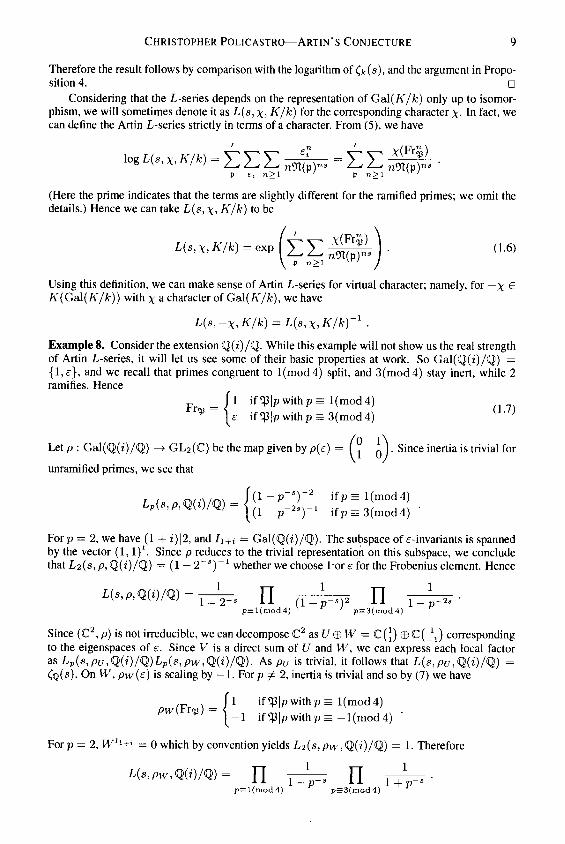
Considering that the L-series depends on the representation of Ga\(K/k) only up to isomorphism, we will sometimes denote it as L(s, x, K/k) for the corresponding character x- In fact, wecan define the Artin L-series strictly in terms of a character. From (5), we have
p S i n > l V r / p n > l K r j
(Here the prime indicates that the terms are slightly different for the ramified primes; we omit thedetails.) Hence we can take L(s,x, K/k) to be
L ( S , X , T O = e x p ^ i : ^ ) - ( 1 - 6 )Using this definition, we can make sense of Artin L-series for virtual character; namely, for — x GK(Gal(K/k)) with x a character of Gal(K/k), we have
L(s,-x,K/k) = L(s,X,K/k)-1 .Example 8. Consider the extension Q(i)/Q. While this example will not show us the real strengthof Artin L-series, it will let us see some of their basic properties at work. So Gal(Q(i)/Q) ={l,e}, and we recall that primes congruent to l(mod4) split, and 3(mod4) stay inert, while 2ramifies. Hence
( l i f q } | p w i t h p - l ( m o d 4 )v \ e i f < P | p w i t h p E E 3 ( m o d 4 ) { }
Letp: Gal(Q(z)/Q) -> GL2(C) be the map given by p(e) = (- n ). Since inertia is trivial for. 1 0unramified primes, we see that
L p ( s , p , Q ( i ) / Q ) = ^ n 2 x( l - p ~ s ) - 2 i f p = l ( m o d 4 )(l-p-28)'1 ifp = 3(mod4) '
Forp = 2, we have (1 4- i)\2, and h+i = Gal(Q(z)/Q). The subspace of ^-invariants is spannedby the vector (1,1)*. Since p reduces to the trivial representation on this subspace, we concludethat L2(s, p, Q(i)/Q) = (1 - 2~s)_1 whether we choose 1-or e for the Frobenius element. Hence
l ^ q w / q h ^ n ( r r ^ i n r ^ -p = l ( m o d 4 ) v ^ ' p = 3 ( m o d 4 ) ^
Since (C2, p) is not irreducible, we can decompose C2 as U © W = C(\) © C(_\) correspondingto the eigenspaces of e. Since V is a direct sum of U and W, we can express each local factoras Lp(s,pu,Q(i)/Q)Lp(s,pw,Q(i)/Q)- As pv is trivial, it follows that L(s,pu,Q(i)/Q) =(q(s). On W, pw(e) is scaling by — 1. Forp ^ 2, inertia is trivial and so by (7) we have
xfl if ^|p with p ee 1 (mod 4)Pw( rvj-|__1 if qjjp withp _ _i(mod4) '
For p = 2, WIl+i = 0 which by convention yields L2(s, pw,Q(i)/Q) = 1. Therefore
L ( 8 , P w M i ) / ® ) = n t ^ n- ^ i + v ~ sp = l ( m o d 4 ) p = 3 ( m o d 4 )

1 0 T h e H a r v a r d C o l l e g e M a t h e m a t i c s R e v i e w 3
We notice that the right hand side is the Hecke L-series for modulus 4 • oo and the nontrivialirreducible character of (Z/4Z)*, which we denote as X4- So we conclude that
L ( s , p , Q ( i ) / Q ) = ( q ( s ) L ( s , X 4 ) • ( 1 . 8 )
From this example, we can already see some of the important facts about Artin L-series. In particular, we guess that the L-series corresponding to the trivial representation is merely the zeta functionof k; namely L(s, Xm\,K/k) = Cfc(s). We will have more to say about such basic properties inthe following section.
1.4.2 Functorial PropertiesIn this section, we prove three results that will be crucial to our understanding of Artin L-series. Inparticular, we learn how L-series corresponding to different fields relate to one another.Proposition 9 (Additivity). Ifx and x' are virtual characters ofGal(K/k) then L(s, x+x'> K/k) -L(s,x,K/k)L(s,Xf,K/k).Proof. This follows immediately from (6). We note that rearrangement is allowed since the seriesc o n v e r g e s a b s o l u t e l y , a s w e s a w i n P r o p o s i t i o n 7 . □Proposition 10 (Towers). Let k C K C L be such that K/k is Galois, and let xoea character ofGa\(K/k). Extend x to a character x ofGa\(L/k). It follows that L(s, x , L/k) =L(s,X,K/k).Proof. Let x correspond to a representation (V", p). Let ^P'|^3|p be prime ideals in Ol, Ok, andOk- Gal(L/k) acts on V according to the projection Gal(L/k) -» Gal(K/k). This map inducessurjective homomorphisms D<$> -> D<$ and Ly -+ I<#. So we obtain a surjective homomorphismDy/Iy —> Dqj/Lp that sends Fr^/ to Frqj. Therefore the action of Fr^/ on V1^' is the same asthe action of Fr^ on V1^. This implies that
det (1 - Frr 9t(p)-) |vV=det(l-Fr¥0I(p)-s) \y,v
w h i c h g i v e s t h e r e s u l t . □Lemma 11. Let G be a finite group with H C G a subgroup. IfN<G, and (W, p) is a representation ofH, then
(Indg W)** Ind^HnN)W»™ .
Proof. We will use our function definition of induction to obtain a natural isomorphism. We notethat a ^-function / : G -+ W is N invariant iff f(xr) = f(x) for all r e N, namely, / isconstant on right, and so also left, cosets of N. This holds iff / is a H/(H n Af)-function on G/N.Such a function takes values in WHnN since rf(x) = f(rx) = f(x) for r G H n N. □Proposition 12 (Induced Representations). Let L/k be a Galois extension. For K an intermediatefield, and \ a character ofGa\(L/K), one has
L(s,X,L/K) = L(s,x\L/k)
where X' := Ind^J^^ X-
Proof. Let G — Gal(L/k) and H = Gal(L/K). Suppose that x corresponds to a representation(W, p) of H, and take V to be Ind§ W. Consider a prime p in Ok- Let qi,..., qr be the primesin Ok lying above p, and for each q^, choose a prime ^ in Ol dividing it. We want to show that
L p ( 8 , X \ L / k ) = l [ L q i ( 8 , x , L / K ) ( 1 . 9 )
and will proceed by reducing to the case r — 1, and then the case that p is unramified.

C h r i s t o p h e r P o l i c a s t r o — A r t i n ' s C o n j e c t u r e 1 1
Denote the decomposition and inertia groups of ^ over p by Di and U. We see that D[ :=H n Di and ![ \— H D U are the decomposition and inertia groups of *}3i over q*. As G actstransitively on the primes lying above p, we can choose elements n G G such that t"1^ = tyi.Since H acts transitively on the primes dividing each q», we note that the set {n \ 1 < i < r} is asystem of representatives for the double cosets Di \ G/H.
We recall that A = r^Din, h = r^hn, and r"1 FrVl r. = FrVi. For /* the residualdegree of q* over p, we know that 9t(q0 = ^(p)^, and Fr£. is a Frobenius element of tyi over
To reduce to the case of r = 1, we will use Mackey's theorem. We can take
Lp(s,x,L/k) = d e t ( l - F V V l « n ( p ) - ) l v ' iSince Fr^ G L>i, this can be rewritten as
Lp(s,X',L/k) = (det (1 - FrVl tt(pp) |(ReSDi Indo w)h )"1 .
By Proposition 6, we know that local factors are equivalent under isomorphism. So by Proposition1, we have
Lp(s,X',L/k) = (det(l - FrVl %p)-° | ©(^nr,^-' nW)h) Jr
= rj(det(l - Fr.Vl 9t(p)- J (Ind£ __, r^)'1))"1 .i = l * *
We can conjugate each factor by r~* to obtain
Lp(s,X',L/k) = n(det(l - r"1 FrVl r^pp | (Ind'C!"1^ HO7'"''1"))-1r
= n(det(! - n*< *(P)~5 I (Ind§ WT ))"1.z = l
Therefore (9) can be rewritten as
n(det(l-Fr^*(p)-s I (Ind^W)1^))-1 = Y[L,t(s,x,L/K)i = l * i = l
= n(det(l-F4^(p)-^s)|vv7,)"1 .i = l
This equation will follow from equality of the ilh factors on either side. So without loss of generality, assume that r = 1. We are left showing that
(det(l - FVV. m(p)~s | (Ind£j Vy)^))"1 = (det(l - FV* ^(p)"^s | W^))"1
for all i. By Lemma 11, this can be rewritten as
(det(l - ErVi np)~S I (Ind^/J] W^)))"1 - (det(l - Rr* <tt(p)-'*s | t^'))"1 (1.10)
If we can convince ourselves that equation (10) corresponds to the tower LDi c LD*7i c L7i,then we can further assume that p is unramified.

12 The Harvard College Mathematics Review 3
In this case, we have Gal(L77LD*) £ Di/U, and Gal(L77LD^) * D'Ji/h ^ D^/IlThe latter isomorphisms let us make sense of W1* as a representation of Gal(L7i/LD' h). Let
Qd :=. Old, H %, QD,t := OlDJ/. n<ft, Qj := £>L/Z n % -
Since
fSL = \Lh : LD*} = Card(A//0 = ff\ /^„ = [^ : ^''l = Card(D{//0 = /*'
we find that f^'1 = fi. Note that 9t(p) = 0I(QD), and that the Frobenius element of Q/ overQd is FrVi. We conclude that for the sake of proving (10), we can take p, q», and q?i to be QD,£}D//,and£}/.
Keeping the initial notation, we can assume that *}3 is the only prime in Ol dividing p, andthat it is unramified. We have that G = Gal(L/k) is generated by FV«p, and H = Gal(L/K) isgenerated by Fr^ for / := /pq = [G : H]. Using our extension of scalars definition of induction,we have that
/ - iV = @FvlvW.
i=0
Let A be the matrix of Fr^ with respect to the basis wi,... ,Wd of W. If I is the d x d unit matrix,then
/ 0 • • • 0 A \I • • • 0 0
\ 0 . . . / 0 /
is the matrix of Fr*p with respect to the basis {Fr^ Wj} of V. This yields
det(l-Fr^9T(p)-s |V) = det-01(p)-s7
V -vi(prsi
-Vl(p)-SA\0
/
(1.11)
Now multiply the first row by ^(p) s and add it to the second, and then multiply the second rowby 9I(p)~s and add it to the third, and so on. Continuing in this way, we see that the determinanto f t h e m a t r i x i n ( l l ) i s d e t ( l - F r j [ J 9 t ( p ) ~ s / ) \ W - □
Consider the character Xtriv of Gal(K/k) induced from the trivial character Xtriv of the subgroup {1}. By Frobenius reciprocity we have
(Xtriv,^) Gal(K/fc) (Xtriv,ReS{i}^){ = V(l)
for each xp G Gal(K/k). Hence xtriv = X^ggTi(k//c) ip(l) • V>- So by Propositions 9 and 12, weobtain the following result.
Corollary 13. <*(,) = <*Wn*eSa(*/*>\{i} L{s^,K/k)^\Given that each L(s,ip,K/k) could be extended to an entire function, we would have the
sought after generalization of Weber's result on abelian extensions! This remains conjectural, however, as we will soon discuss.

C H R I S T O P H E R P O L I C A S T R O — A R T I N ' S C O N J E C T U R E 1 3
1 . 4 . 3 A b e l i a n C h a r a c t e r s . . . .Havine described some of the basic properties of Artin L-series, we want to know their relation toS^e!^Sular, we Jght wonder whether an Artin L-series attached to an abeliancSci gW us aTecke Series8 This seemed plausible to Artin who needed *-relate totTorization of <K(S) (cf. Corollary 13) to Weber's factorization of Ck(s) in the case that K/k is
"Sbs/t/on id<*tiirF**"« JCJs a class field for some class group CT /jf/. Moreover, he knewProposition l4(Artm Kec.proc.ty,. ^j «««»m««wa-4u,)«x'flw-ni^m^:§.SqiB^on_ _Pf in its kernel.
nf n lf^f™ °f thiS "dual f0rm" of Artin Re^procity see [7]. Let v be an abelian charactero'Gal(K/k) Composing with the Artin symbol, and noting that Ms ma ffactors through /"/?'simenJof SSi ? ChTT, m°f ° f °f thC ^ d3SS ^ This iws ™ «» Sve a Predsestatement of the relation of abelian L-series to nonabelian L-series.
iSomt? ( /l X 'heCOrresP°ndi»8character ofCI*. For S := {p|f | X(IV) = 1},L(s,x,K/k) = L(s,x')T[ 1
then C v = {0}. So the corresponding local factor is 1. If p|f and X(IV) = 1, then
L P ( s , x , K / k ) = *i - x(Fvv)«n(p)- •Hence
L ( s , x , t f / A ) = T T F T 1pt| 1 - X(ttv)9t(p)- 11 i _ x(FVv)OT(p)- •
We recall that
By construction *'(p) = x ((*£)). Therefore X'(p) = x(F^). This gives the result. □

1 4 T H E H a r v a r d C o l l e g e M a t h e m a t i c s R e v i e w 3
a-w = L(a,x')j]rP„- w(p)-.-
^ ( - S ^ t 0 * " * * * * C — 1 3 . w e c a n
C q ( o ( « ) = C q ( * ) £ ( « , X 4 ) . ( 1 1 2 )
1 . 4 . 4 M e r o m o r p h i c C o n t i n u a t i o n . ^ _ • . .
1.5 Artin's ConjectureRecall that the starting point of Artin's investigation of nonabelian L-series was the question ofwhether {*-(*)/&(*) was an entire function for K/k a nonabelian Galois extension. By Corollary13 and Theorem 17, we see that Cx(s)/Cfc(s) extends to a meromorphic function on C. The resultsdiscussed do not, however, let us conclude that this extended function lacks poles. The difficultyis that, in the notation of Theorem 17, Brauer's theorem does not tell us which m are positive, orwhich Vi are nontrivial. Artin believed though that his nonabelian L-series could be analyticallycontinued, given that the character \ did not contain any copies of xt™; namely, he made thefollowing conjecture.
Artin's Conjecture. For K/k a Galois extension, and \ a nontrivial irreducible character,the Artin L-series L(s, \, K/k) extends to an entire function.
Though progress has been made on this conjecture, it remains an open question. Before discussing some present work on this problem, let us note a class of Galois groups for which it is true.Suppose that Gal(K/k) is a monomial group, that is, each irreducible character \ of Gal(K/k) isinduced from an abelian character </>' of some subgroup H. This would include, for instance, thecase that Gal(K/k) is a p-group for some prime p.
C h r i s t o p h e r P o l i c a s t r o — A r t i n ' s C o n j e c t u r e 1 3
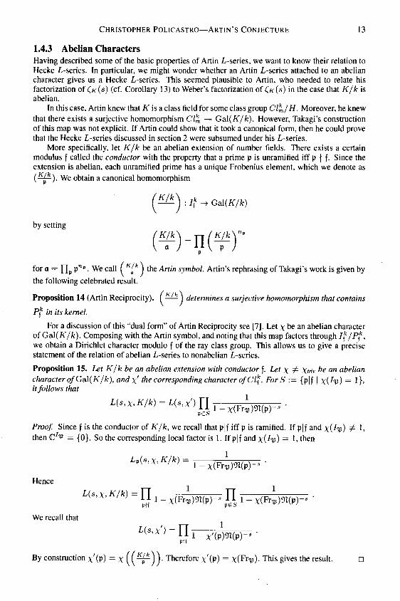
1.4.3 Abelian CharactersHaving described some of the basic properties of Artin L-series, we want to know their relation toHecke L-series. In particular, we might wonder whether an Artin L-series attached to an abeliancharacter gives us a Hecke L-series. This seemed plausible to Artin, who needed to relate hisfactorization of (k(s) (cf. Corollary 13) to Weber's factorization of £k(s) in the case that K/k isabelian.
In this case, Artin knew that K is a class field for some class group Cl /H. Moreover, he knewthat there exists a surjective homomorphism C/£ -» Gal(K/k). However, Takagi's constructionof this map was not explicit. If Artin could show that it took a canonical form, then he could provethat the Hecke L-series discussed in section 2 were subsumed under his L-series.
More specifically, let K/k be an abelian extension of number fields. There exists a certainmodulus f called the conductor with the property that a prime p is unramified iff p \ f. Since theextension is abelian, each unramified prime has a unique Frobenius element, which we denote as(^p). We obtain a canonical homomorphism
by setting
f ___A : /* _> Gal(K/k)
(M)_n(^vfor a = Y\p Pnp • We call ( ^p J the Artin symbol. Artin's rephrasing of Takagi's work is given bythe following celebrated result.
Proposition 14 (Artin Reciprocity). ( —*— j determines a surjective homomorphism that containsPffc in its kernel.
For a discussion of this "dual form" of Artin Reciprocity see [7]. Let x be an abelian characterof Gal(K/k). Composing with the Artin symbol, and noting that this map factors through if/Pf,we obtain a Dirichlet character modulo f of the ray class group. This allows us to give a precisestatement of the relation of abelian L-series to nonabelian L-series.Proposition 15. Let K/k be an abelian extension with conductor f. Let x ¥" Xtriv be an abeliancharacter of Ga\(K/k), and x' the corresponding character of Cif. For S := {p|f | x(Iv) = 1}>it follows that
Proof. Since f is the conductor of K/k, we recall that p|f iff p is ramified. If p|f and x(Iy) / 1.then C/$p = {0}. So the corresponding local factor is 1. If p|f and x(?v) = 1»tnen
Lp(s,X,K/k)l -x (Frv)9 I (p) - * '
HenceHs, x, K/k) = yi ______ rj _____.
We recall that
L(s'x')=ni-x'(PW)--By construction x(p) = X ((^))- Therefore x'(p) = x(Fr^). This gives the result.

1 4 T h e H a r v a r d C o l l e g e M a t h e m a t i c s R e v i e w 3
So if x is injective, then S = 0, and we conclude that L(s, x, K/k) = L(s, x')- In tne casethat x = Xtriv, then \' is the trivial character modulo f, and we see that
CK{s) = L(s,x')Y[r^{P l f K r j
Example 16. Let us see how the previous results apply to Example 8. By Corollary 13, we canreplace L(s, p, Q(i)/Q) by Cq(o(5) in (8)t0 obtain
C q ( z ) W = C q ( s ) L ( s , X 4 ) - ( 1 . 1 2 )
Since the discriminant of Q(i)/Q is 4, we know that the finite part of the conductor is either 2or 4. We know that a prime p > 0 splits completely iff p = l(mod4). So f = 4 • oo withCZ^oo — (Z/4Z)* by Example 3. Hence Proposition 15 explains why X4 appears in expression(12).
1.4.4 Meromorphic Continuation.Having connected Artin L-series to Hecke L-series, we can use Proposition 5 to meromorphicallyextend Artin L-series to the plane.Theorem 17. Let L/k be a Galois extension, and x a character ofGal(L/k). The Artin L-seriesL(s,x, L/k) admits a meromorphic continuation to C.Proof. By Theorem 2, we can express \ as X = YhLi n* * Inc*Hz ^ for m £ ^> where Hi c Gare subgroups, and xpi is abelian. By Proposition 9 we obtain
m
L(s, x, L/k) = fj L(s, Indg, Vi, L/fc)n' .1 = 1
By Proposition 12, we have L(s,Indtf. ipi,L/k) = L(s,ipi,L/Ki) where K* is an intermediate field such that GaI(L/A'i) = h\. By Proposition 15 and Proposition 5, we know thatL(s, ipi, L/Ki) can be meromorphically continued to C. This gives the result. □
Phew! Artin was unable to prove Theorem 17, though he made progress on it by showing aweaker version of Brauer's theorem. He proved that a character of a finite group can be expressedas a Q-linear combination of characters induced from abelian characters of subgroups. So clearingdenominators, he concluded that a sufficiently large power of the L-series admitted a continuation.
1.5 Artin's ConjectureRecall that the starting point of Artin's investigation of nonabelian L-series was the question ofwhether CtfM/CfcW was an entire function for K/k a nonabelian Galois extension. By Corollary13 and Theorem 17, we see that Of W/Cfc(s) extends to a meromorphic function on C. The resultsdiscussed do not, however, let us conclude that this extended function lacks poles. The difficultyis that, in the notation of Theorem 17, Brauer's theorem does not tell us which m are positive, orwhich fa are nontrivial. Artin believed though that his nonabelian L-series could be analyticallycontinued, given that the character x did not contain any copies of XtnV; namely, he made thefollowing conjecture.
Artin's Conjecture. For K/k a Galois extension, and x a nontrivial irreducible character,the Artin L-series L(s,x,K/k) extends to an entire function.
Though progress has been made on this conjecture, it remains an open question. Before discussing some present work on this problem, let us note a class of Galois groups for which it is true.Suppose that Ga\(K/k) is a monomial group, that is, each irreducible character x of Ga\(K/k) isinduced from an abelian character i/j' of some subgroup H. This would include, for instance, thecase that Gal(K/k) is a p-group for some prime p.
C h r i s t o p h e r P o l i c a s t r o — A r t i n ' s C o n j e c t u r e 1 5
From Frobenius reciprocity, we see that if \ is nontrivial, then xp' is nontrivial. By Proposition12, we know that that L(s, x, K/k) = L(s, xp', K/KH). If N C H is the kernel of xp', thenby Proposition 10, we have that L(s, xp', K/KH) = L(s, xp, KN/KH) where xp : H/N <-+ C*.So by the remark after Proposition 15, and Proposition 5, we conclude that L(s,xp,KN/KH)analytically extends to C. Therefore Artin's conjecture holds for monomial Galois groups.
What stinks is that not every group is monomial.
1.5.1 Langlands programWhile Artin was able to prove many important analytic properties of his nonabelian L-series, andconnect them to abelian L-series using his reciprocity theorem, he was unable to give the appropriate n-dimensional analogues of Dirichlet characters and L-functions. Although at the time, Heckewas researching such functions in the case of n = 2, it remained for Robert Langlands many yearslater to see a connection, and provide some precise statements. His vast set of conjectures offernot only, a solution to Artin's conjecture, but a synthesis of many of the classical ideas in numbertheory.
We will very roughly describe Langlands' insight. For a more detailed survey the reader shouldsee [2, Sec. IIIJV] and [4, Sec. 7]. Given a place v ofk, let kv denote the corresponding completionwith valuation ring Ov- Let Gn(A) be the subgroup of Ylv GLn(ku) formed by tuples (gu) suchthat gu € GLn(Ou) for all but finitely many v. Suppose 7r is an irreducible unitary representationof Gn (A) in some Hilbert space Hw. By defining local factors for almost all primes, Langlandsdescribed an L-series L(s,n) given by their product. Jacquet and Langlands then proved thatfor arbitrary n, local factors could be added so that the product could be taken over all primes.Moreover, if n takes a certain form, they were able to show that L(s,ir) extends to an entirefunction, unless n = 1 and n is trivial. Motivated by a search for a sort of converse to this result,Langlands made the following conjecture.
Langlands' Reciprocity Conjecture. Let K/k be a Galois extension, and cr : Gal(K/k) ->GLn(C) an irreducible n-dimensional representation. There exists a representation ira ofGn(A)such that L(s, ira) = L(s, cr, K/k).
When n=l and K/k is abelian, this conjecture reduces to Artin's reciprocity theorem. Forarbitrary n, the truth of this result would imply Artin's conjecture.
As we will see in the next section, there appear to be other ways of arriving at Artin's conjecture. But given the scope of the Langlands program, this route would be a momentous achievementfor number theory.
1.5.2 Selberg conjecturesIn the course of this paper, we have seen several different constructions of L-series. The similarities of these constructions lead us to wonder whether we could study a broadly defined familyof L-functions, rather than a single construction. These sorts of concerns led Alte Selberg to ax-iomatically define a class S of L-functions. Elements F(s) e S are complex valued functionsof a complex variable that satisfy several of the properties we have discussed; they should be rep-resentable as a series for Re(s) > 1, but also have an expression as a product, and they shouldmeromorphically extend to the plane.
Since S is multiplicatively closed, Selberg wanted some notion of factorization and irreducib-lity. He called a function F e S primitive if the equation F — FiF2 for Fi,F2 e S implieseither F = F\ of F = F2. It can be shown that each element of S factors into a product ofprimitive functions. The uniqueness of this factorization would be among several consequences oftwo conjectures made by Selberg. For statements, we refer the reader to [4, Sec. 1].
Using the Chebotarev density theorem, and the basic properties of Artin L-series developedhere, it is easily shown that unique factorization implies Artin's conjecture. For a proof of this fact,and a more detailed discussion of the relation of Selberg's conjectures to Artin's and Langlands'conjectures see [4].
1 6 T h e H a r v a r d C o l l e g e M a t h e m a t i c s R e v i e w 3
AcknowledgementsThe author would like to thank Keith Conrad for suggesting several revisions to this paper, and alsoCarl Erickson and Ben Brubaker for helpful discussions.
References[l] E. Artin, Uber eine neue Art von L-Reihen, Collected Papers, Springer, 1965.
[2] S. Gelbart, An Elementary Introduction to the Langlands Program, Bull. A.M.S. Vol. 10,No. 2 (1984), 177-220.
[3] W Fulton and J. Harris, Representation Theory, Graduate Texts in Mathematics, Springer,2004.
[4] M. R. Murty, Selberg's Conjecture and Artin L-functions, Bull. A.M.S. Vol. 31, No. 1 (1994),1-14.
[5] J. Neukirch, Algebraic Number Theory, Grundlehren der mathematischen Wissenschaften,Springer, 1999.
[6] J.P. Serre, Linear Representations of Finite Groups, Graduate Texts in Mathematics, Springer,1971.
[7] J. Tate, Problem 9: the general reciprocity law, Proc. Sympos. Pure Math., A.M.S., Vol. 28(1976), 311-322.

STUDENT ARTICLE
Hilbert's Nullstellensatz and SchemesMiles Dillon Edwards*Indiana University '13
Bloomington, IN [email protected]
AbstractWe prove Hilbert's Nullstellensatz from a geometric perspective, and use it to motivate the beginnings of scheme theory.Disclaimer. In the rest of this paper, "ring" is shorthand for "commutative ring with unit".
2.1 Introduction, Statement, and Start of ProofIn differential geometry, we study manifolds—spaces that look like Rn in small neighborhoods.The simplest kinds are curves and surfaces. Level sets of smooth functions are also manifolds(possibly with singularities). So are the solution sets of systems of equations involving smoothfunctions.
In algebraic geometry, we study algebraic analogs. The classical objects of study are calledalgebraic varieties. These are solution sets to systems of algebraic equations, i.e., common zeroesof polynomials over some field K. Familiar examples include finite collections of lines, planes,hyperplanes, and even points, as well as conic sections, quadric surfaces, elliptic curves, and graphsof polynomials. We can consider solutions in different contexts. We may consider solutions inaffine n-dimensional K-space, that is, Kn. However, it is often convenient to work in projectivespace, which allows certain statements that are "almost always" true (e.g., "any two distinct linesmeet in one point") to become statements that are always true. Still, projective space is "locally"affine, in the sense that every point has a neighborhood (in fact, quite a large one—almost the entirespace) that looks like affine space.
One pleasing result from classical algebraic geometry is Bezout's Theorem ([6], III.2), whichsays (in its elementary form) that any two curves of degrees ra and n (in a projective plane overan algebraically closed field) meet in ran points, if multiplicity is counted carefully. This seemsintuitive—after all, it matches the case where the curves are just collections of lines. However, itis not easy to prove, in part due to the fact that it is tricky to define multiplicity of intersection in aprecise way. Another charming result is the fact that every cubic surface in projective space (overan algebraically closed field) contains 27 lines ([3], V.4).
Hilbert's Nullstellensatz is a result (or collection of results) that connects n-dimensional affineif-space (where K is an algebraically closed field) with its ring of (polynomial) functions in aprecise and intimate way. Without further ado, we present the theorem—or at least, one version ofthe theorem.Theorem 1 (Hilbert's Nullstellensatz, Version 1). Let K be an algebraically closed field. Then themaximal ideals of the ring K[x\,... ,xn] are precisely of the form I(p), where I(p) denotes theset of polynomials that vanish at the point p in n-dimensional K-space.Start of proof. We first note that I(p) is always a maximal ideal of K[xi,... ,xn], as it is infact the kernel of the evaluation map K[xi,...,xn] -+ K that evaluates polynomials at p. Thismap is clearly surjective, as K[xi,. ..,xn] contains all the constant polynomials. It follows that
t Miles Dillon Edwards is a sophomore studying mathematics and cello performance at Indiana University.He has taught at PROMYS and works for the Art of Problem Solving. He has particular interest for grouptheory, number theory, and most things algebraic.
17

1 8 T h e H a r v a r d C o l l e g e M a t h e m a t i c s R e v i e w 3
K[xi,...,xn]/I(p) is a field isomorphic to K, so I(p) is maximal. It thus remains to show thatevery maximal ideal of K[xi,..., xn] arises in this way.
This is the difficult part of the proof, but it is plausible. If we have a maximal ideal I ofK[xi,. ..,xn), then the quotient field K[xi,..., xn]/I is canonically a field extension of K. Thisis suspicious, because K is supposed to be algebraically closed, and we are only working withfinitely many variables. The only way things could possibly go wrong would be if we somehow gota transcendental extension of K. This seems highly unlikely, as such an extension would have tocontain a transcendental t, as well as 1/P(t), for every nonzero polynomial P. Our proof involvesa little more work, as we could have an extension that is not purely transcendental, but this is themain idea.
2.2 Rings of Integers and the End of the ProofWe now develop some commutative algebra that will be familiar to students of algebraic numbertheory.Definition 2. Let A be a subring of a ring B. An element x of B is integral over A if it is a zeroof a monic polynomial with coefficients in A; that is, if there are elements ao,..., an_i in A suchthat
xn 4- an-ix71'1 H h aix + ao = 0.
The motivation for this terminology comes from number theory, where B is usually a numberfield (i.e., a finite extension of the field of rationals) and A is usually Z, the ring of ordinary integers.In this case, the algebraic integers are the zeroes of monic polynomials with integer coefficients.
It turns out that the elements of B that are algebraic over A constitute a ring, called the integralclosure of A (in B). Furthermore, if B has no zero divisors, then every element of B that isalgebraic over A is equal to some x/a, where x is an integer over A and a is an element of A. Wenow prove these facts.
Proposition 3 (Criterion for Integrality). Let B be an extension of a ring A. An element x of B isintegral over A if and only if A[x] (a subring ofB) is finitely generated as an A-module.Proof. First, suppose that A [x] is a finitely generated A-module. Consider the ascending chain ofsubmodules
AcA + AxcA + Ax + Ax2 C • • • .
The union of this chain is the entire module A[x\. On the other hand, A[x] is finitely generated.Thus if we fix a generating set, then there must be some finite n such that A + Ax-\ h Ax71'1contains each of the elements of the generating set of A[x\. But then this submodule A + Ax +
h Axn~x must be equal to A[x]—in particular, there must exist elements ao,. ..,an-i of Asuch that
n i i i n — 1x = ao + aix + h an-ixIt follows that x is integral over A.
Conversely, suppose that x is integral over A. Let
xn + an-ixn~l -\ ha0
be a monic polynomial in x which evaluates to zero. Then from the polynomial division algorithm,every element of A[x] is equal to some polynomial in x of degree at most n—1, with coefficientsin A. Thus A[x] is generated by the f in i te set {1, x1, . . . , xn~1}. □
The next proposition resembles a familiar result from field theory, that dimension of field extensions is multiplicative.
Proposition 4. Let B be a ring, and let Abe a subring ofB. Let C and D be subrings ofB thatcontain A.IfC and D are finitely generated as A-modules, then so is CD, the least subring of Bcontaining C and D.

Miles Dil lon Edwards—Hilbert 's Nul lstel lensatz and Schemes 19
Proof Let {ci,..., cm} be a generating set for C, and let {di,..., dn } be a generating set for D.We claim that the elements of the form ddj generate CD as an ^-module. To this end, we notethat the elements of CD are the elements of B that are sums of elements of the form cd, for cin C and d in D. It thus suffices to show that every element of the form cd lies in the submodulegenerated by the Cidj. For this, we note that for any c in C, there are elements ai,... ,am of Asuch that m
c = } a j C j ;i = l
similarly, for any d in D, there are coefficients a[,..., a'n such thatn
3 = 1
Then we havecd = ^ aid ^2 a'jdo = y^^(aia'j)cidj,
i j i , j
which lies in the submodule spanned by the Cidj. Thus the set of elements of the form adj generateCD as an A-module; since the generating set in question is finite, we are done. □
Now we get the result we wanted from the previous two propositions.Definition 5. A ring A is Noetherian if one of the following equivalent conditions is satisfied:
• Every ascending chain jof ideals Io C h C • • • is eventually constant.
• Every ideal of A is finitely generated.
• Every submodule of a finitely generated A-module is finitely generated.
Proposition 6 (The Set of Integral Elements is a Ring). Let Abe a subring of a ring B. Then theset of elements ofB that are integral over A constitute a ring.
Proof. Though this proposition is true generally, it simplifies the proof (and is sufficient for ourpurposes) to deal with the case where the ring A is Noetherian.
Suppose that x and y are integral over A. Then A[x] and A[y] are finitely generated A-modules.Since A[x] = A[—x], it follows that — x is integral over A. Now, x + y and xy both belong toA[x, y], which is the subring of B generated by A[x] and A[y\. But the ring A[x, y] is a finitelygenerated ^-module, by proposition 4. Since A is Noetherian, the submodules A[x + y] and A[xy]are also finitely generated. Therefore x + y and xy are integral over A. This gives us what wew a n t e d . □Proposition 7 (All Algebraic Elements Arise from Integral Elements). Let B be a ring, and let Abe a subring ofB. Let y be an element ofB that is algebraic over A. Then there is some nonzeroelement a of A and some element x ofB, integral over A, such that x = ay.Proof. By definition, there are some elements ao,... ,an such that
5_a = 0'i=0
with an 7^ 0. Let x = any. Then we haven n — 1
i = 0 i = 0 i = 0
Then x is integral over A, and x = any, where an belongs to A, as desired.

2 0 T h e H a r v a r d C o l l e g e M a t h e m a t i c s R e v i e w 3
We finish with a result that allows us to determine concretely whether elements of B are integralover A, if B is a field.Proposition 8 (Concrete Criterion for Integrality). Let B be afield, and let Abe a subring ofBwhich is a unique factorization domain. Let C be the field of fractions of A. Then an element xof B is integral over A if and only if it is algebraic over C, and all the coefficients of its (monic)minimal polynomial (over C) lie in A.
Proof. It is clear that if the latter condition holds, then x is integral. For the converse, suppose that xis integral; then by definition, x is algebraic over C. Let / be the (monic) minimal polynomial of #,and let h be a monic polynomial with coefficients in A such that h(x) = 0. Then there must besome a with coefficients in C such that fg = h. But by Gauss's lemma, both / and g must havecoefficients in A. In particular, /, the minimal polynomial of x, has coefficients in A. □Conclusion of the Proof of the Nullstellensatz. Suppose for the sake of contradiction that / is anideal of K[x\,..., xn] such that K[x\,..., xn]/I is a transcendental extension L of K. We picka transcendence base ti,...,tk for L, i.e., a maximal set of elements with no polynomial relationsamong them. (We can even take the U to be a subset of the Xi. For more details on transcendencebases, we refer the reader to section VIII. 1 of [4].) Then L is an algebraic (in fact, finite) extensionof the purely transcendental extension K(t\,..., tk). Let A be the subring K[ti, ...,£&]. Then Ais a unique factorization domain. (The interested reader may find a proof of this fact in Theorem 2.3of [4], in chapter IV, related to Gauss's lemma.) It is also a Noetherian ring, by Hilbert's BasisTheorem ([1], 7.5; [4], section IV4). Since all algebraic elements in this situation arise fromintegral elements, every element of L is of the form x/a, where x is integral over A and a is anelement of A, i.e., a polynomial in ti,..., tk with coefficients in K.
Now, let ai,..., an be nonzero elements of A such that the elements _*_* (of L) are all integralover A. We claim that the ai cannot all be units (i.e., elements of K)—indeed, otherwise, the Xi(or rather, their images in L) would all be algebraic integers over A, so all the elements of L wouldbe integral over A. This implies in particular that 1/ti is not in L, as its minimal polynomial isP(z) = z — 1/ti, in violation of our concrete criterion for integrality. Thus the a* are not allunits—that is, they are not all constant polynomials. Then their product _i • • • an is not constant,so ai • • • an + 1 is not zero. Consider, then, the element
1ai • • • on + 1
of L. Since L is a quotient of K[x\,..., xn\, this element must be equal to some polynomial in_ i,..., xn- It follows that there must be non-negative exponents ei,..., en such that
ai • - an + 1
is integral over A = K[ti,..., tk]- But this cannot be—indeed, this element belongs to the fieldof fractions of A, but not to A (since the numerator and denominator have no common factors, andthe denominator is not a unit). Therefore it cannot be integral over A, from our concrete criterion.Th is i s a con t rad ic t i on , so L mus t be an a lgebra ic ex tens ion . □
If we examine our methods carefully, we see that we only used the algebraic closure of K whenwe noted that all algebraic extensions of K are trivial. Thus the following, slightly more generalversion of the theorem is true.Theorem 9 (Hilbert's Nullstellensatz for a General Field). Let K be afield, and let I be a maximal ideal of the polynomial ring K[x\,..., xn\- Then the quotient K[xi,..., xn]/I is a finiteextension ofK.
2.3 The Strong FormThe Nullstellensatz we have given is called the "weak version". The "strong version" is as follows.
Miles Dil lon Edwards—Hilbert 's Nullstel lensatz and Schemes 21
Theorem 10 (Hilbert's Nullstellensatz, Strong Version). Let K be an algebraically closed field,and let a be an ideal of K[x\,..., xn]. Let V (a) be the variety in Kn of points at which all theelements of a vanish. Then the ideal of elements that vanish on V(a) is the radical of a.
We recall that the radical of an ideal a is the collection of elements a such that an belongs to afor some positive n; it is an ideal, and it is sometimes denoted r(a), or y/a. If we use I(V) todenote the ideal of elements vanishing on a variety V, then we can express the strong form as apithy equation :
I(V(a)) = ^~a.
In our proof, we use the fact that the radical of an ideal is the intersection of the prime idealscontaining that ideal. This is equivalent to the statement that the nilradical of a ring (i.e., thecollection of nilpotent elements) is the intersection of the ring's prime ideals. We prove this fact inour appendix; the reader may also refer to [1], chapter 1.
Proof of the Strong Version. It follows from our definitions that if fn belongs to a, then / mustvanish at every point in V^a). Thus the radical of a is a subset of the ideal of V(a), so it suffices toshow that the opposite inclusion holds. This reduces to showing that if / is a polynomial that vanishes on K[xi,..., xn], then / belongs to every prime ideal containing a, from the characterizationof the nilradical of the ring K[xi,..., xn]/a.
To this end, let p be a prime ideal containing a, and let q be the ideal generated by p in thering K[xi, ...,xn,y\- We note that the variety of the ideal (q, 1 - yf) has no points (in Kn+1);indeed, if a point vanishes under all the elements of q, then it must vanish under /, so 1 — yf mustevaluate to 1. By the weak version of the Nullstellensatz, this means that there is no maximal idealthat contains (q, 1 — yf), so K[xi,... ,xn,y]/(c\,l — yf) must be the zero ring. But this ring isjust the localization of the ring K[x\,..., xn]/p by the element /. Since this quotient ring has nozero divisors (as p is a prime ideal), this means that / must be zero in this ring—that is, p mustc o n t a i n / . □
This theorem shares its name with the "weak" form because the weak form follows from thestrong form thus: if an ideal a has no points on its variety, then its radical must be the collectionof polynomials that vanish on the empty set, which is (vacuously) the collection of all polynomialsin our ring. In particular, a cannot be a maximal (proper) ideal, as its radical is the unit ideal; itfollows that the only maximal ideals are those that arise from points.
As we have seen, the other direction is not as easy. The idea of introducing a variable y to standfor 1// is called the Rabinowitsch trick, after J. L. Rabinowitsch, who published it in a one-pagepaper in 1929. There are many ways of proving the weak form of the Nullstellensatz, but modernproofs of the strong form seem, as a rule, to deduce the strong form from the weak form using thistrick. Curiously, little seems to be known about Rabinowitsch—he is not currently listed in theMathematics Genealogy Project. Rabinowitsch's paper was apparently submitted from Moscow,but this author has not succeeded in finding any other information about him.
The method is called a "trick", but it seems a little less arbitrary if we are aware of the Jacobsonradical of a ring R, which is both the intersection of all maximal ideals of R and the collection ofelements x such that 1 — yx is invertible for every element y of x ([1], ch. 1). We know that /belongs to the Jacobson radical of K[xi,..., xn]/a, and we want to wreak havoc on any primeideals p to which / does not belong. And what could cause greater havoc than requiring 1 — yf tobe zero, when it is supposed to be invertible?
2.4 Historical AsideThe German word Nullstellensatz roughly means "theorem of the zeroes". The reason for this namebecomes more apparent if we state the classical versions of the theorems. These are equivalent tothe versions we have seen so far; they have the advantage of making the theorem appear morestriking and making the connection between the two versions more apparent, but the disadvantageof obscuring the geometric intuition.

2 2 T h e H a r v a r d C o l l e g e M a t h e m a t i c s R e v i e w 3
Theorem 11 (Hilbert's Nullstellensatz, Classical Weak Form). Let K be an algebraically closedfield, and let f\,..., fT be polynomials in n variables over K. Then either the fi have a commonzero, or there exist polynomials gi,..., gr such that
_ 9ifi = 1.l < i < r
Theorem 12 (Hilbert's Nullstellensatz, Classical Strong Form). Let K be an algebraically closedfield,and let fi,..., fr be polynomials in n variables over K. Let f be another such polynomial.If f vanishes on all the common zeroes of the fi, then there exist polynomials gi,... ,gr and aninteger ra such that
_ 9ifi = r.l < i < r
When we express the theorems like this, the weak form is the special case of strong form where/ is the constant polynomial 1.
2.5 Varieties and SchemesHilbert's Nullstellensatz gives us some hope of expressing results from algebraic geometry morepurely in the language of commutative algebra—points correspond to maximal ideals, and moregenerally, sub-varieties correspond to (radical) ideals. We can think of a ring of the form
K[x i , . . . ,xn} /a
as the ring of functions on the variety V(a). Maximal ideals of this ring correspond to maximalideals of K[x\,..., xn] that contain the ideal a—i.e., points on the variety of a. In general, idealscorrespond to sub-varieties.
But why limit ourselves to finitely generated rings over algebraically closed fields? It is sometimes useful to work over fields that are not algebraically closed—indeed, in number theory, weoften want to work over Q or finite extensions of Q. So we could be tempted to define an abstractvariety as the collection of maximal ideals of an arbitrary (commutative) ring. The problem withthis idea is that ring homomorphisms do not induce convenient general relations between maximalideals of rings. But they do induce nice relations between prime ideals: specifically, the inverseimages of prime ideals under ring homomorphisms are again prime ideals. This motivates the definition of the spectrum of a ring as the set of all prime ideals of the ring; it comes with a topology,where a closed set is the collection of prime ideals containing a given ideal. In the case where ourring is K[xi,..., xn\, these are just the varieties of n-space; intuitively, closed sets of the spectrumare (sub)varieties of the space.
This gives us a generalized notion of affine varieties. For the generalizations of projectivespace and other things, we allow spaces in which every point has a neighborhood isomorphic tosome affine space, i.e., to the spectrum of some ring, in such a way that the isomorphisms. Thisconstruction is done precisely, and in more detail in [3], II. 1-2.
This definition is slightly strange, in part because of the presence of non-maximal prime ideals.These are "points" in the spectrum, but they also define closed sets containing other points. As itturns out, the closed sets they define are irreducible; that is, they cannot be expressed as a unionof two strictly smaller closed sets. We think of these ideals as generic points on these irreducibleclosed subsets. It turns out that this relation is bijective; every irreducible closed subset has ageneric point that is a prime ideal (see [1], ex. 19; [3], III, 3.1).
Another strange aspect of this definition is that our space is endowed with a very weak topology.We have already noted that there may be many "generic" points whose closures contain otherpoints. Our open sets will be very large—after all, in our model case, affine n-space, our closedsets have dimension smaller than the space itself. For example, the spectrum of C[x] consists of thepoints of the complex plane (corresponding to maximal ideals), along with a generic point of theentire space, corresponding to the zero ideal. But the only open sets are those obtained by removing

Miles Dil lon Edwards—Hilbert 's Nul lstel lensatz and Schemes 23
finitely many closed points. This means that, among other things, every injective function from anyHausdorff space into the spectrum of C[x] is continuous, as long as we avoid the generic point! Thisstrange topology makes standard topological tools difficult to use, but certain cohomology theorieshave been developed for use with schemes and related spaces; some of these theories are developedin [3], chapter III. This theory of schemes seems strange at first, but it has been influential, and itlies behind some of the more spectacular recent advances in number theory.
2.6 AcknowledgementsI am indebted to many teachers and friends who have helped me lately. I owe particular debtsto Michael Larsen of Indiana University, and to my parents, Meg Dillon and Steve Edwards, ofSouthern Polytechnic State University.
2.7 Appendix: the NilradicalProposition 13. Let R be a ring. Then the nilradical of R is the intersection of the prime idealsofR-Proofi Suppose first that an element a belongs to the nilradical of R. Then an = 0 for somepositive integer n; it follows that a must be zero in any quotient of R that has no zero divisors.Thus a lies in every prime ideal of R.
Suppose on the other hand that an ^ 0 for every positive integer n. Consider the set S ofideals that avoid all powers of a, ordered by inclusion. This set is non-empty (since it contains thezero ideal), and the union of any totally ordered family of elements of S also belongs to S. ThusS satisfies the hypotheses of Zorn's lemma, so it has a maximal element; let p be such a maximalelement. We claim that p is a prime ideal.
Indeed, suppose that x and y are elements of R such that xy = 0 in R/p. Since p is a maximalelement of S, we know that either p contains x, or the ideal p + (_) contains an for some integer n.Similarly, either p contains y, or the ideal p + (y) contains am for some integer ra.
Suppose that powers of a belong both to p 4- (x) and to p + (y). Then there exist elements dand e of R such that dx = an (mod p) and ey = am (mod p). Then we have
0 ee d;r?/e = am+n (modp),
a contradiction. Therefore one of x and y must belong to p. Thus p is a prime ideal that avoids allpowers of a.
Thus if a does not belong to the nilradical of R, then R has a prime ideal not containing a, sow e a r e d o n e . □
References[1] M. F. Atiyah and I.G. MacDonald: Introduction to Commutative Algebra. Westview
Press, 1969.
[2] D. Eisenbud: Commutative Algebra with a View Toward Algebraic Geometry. New York:Springer, 1999.
[3] R. Hartshorne: Algebraic Geometry. New York: Springer, 1977.
[4] S. Lang: Algebra. New York: Springer, 2002.
[5] J. L. Rabinowitsch: Zum Hilbertschen Nullstellensatz, Math. Ann. 102 (1930) #1, 520.
[6] I. R. Shafarevich (trans. K. A. Hirsch): Basic Algebraic Geometry. Springer, 1977.

STUDENT ARTICLE
Toronto Spaces
Manuel Rivera*Massachussets Institute of Technology '10
Cambridge, MA [email protected]
AbstractA topological space X is said to be a Toronto space if it is homeomorphic to all its subspaces ofthe same cardinality. In this paper, we present some results in the area of set theoretic topologyconcerning these spaces and the so-called Toronto problem, an open question about the existenceof a Toronto space that is uncountable, non-discrete and Hausdorff. We conclude the paper thatsuch a space, if it exists, must be separable (assuming the Continuum Hypothesis).
3.1 IntroductionOne often hears in mathematical circles that the field of point set topology is dead. It is certainly nota popular area of research; however, there are many interesting open problems which are accessibleto young researchers and have connections with other areas of mathematics, such as logic and settheory. In this paper, we present some results and questions about Toronto spaces, assuming onlythe basic notions of point-set topology. We begin by reviewing some preliminary concepts beforedescribing the nature of Toronto spaces.Definition 1. If X is any set, the collection of all subsets of X is a topology on X which we callthe discrete topology. We say a topological space X is non-discrete if there exists a subset of Xwhich is not an open set in X.Definition 2. Let X be a topological space with topology r. If Y is a subset of X, the collectiont' = {Y DO : O e t}\ssl topology on Y, called the subspace topology.
Now, we define our main object of study, which was introduced by J. Steprans in [4]:Definition 3. Let X be a topological space. We say X is a Toronto space if it is homeomorphic toall its subspaces of the same cardinality as X.
In other words, we say a topological space X is a Toronto space if for any subspace Y c Xsuch that \Y\ = \X\, Y is homeomorphic to X (Y _i X).
Note that any set X with the discrete topology is a Toronto space. For if Y C X then thesubspace and the discrete topologies on Y are equivalent. Hence, if \Y\ = \X\, any bijectionbetween X and Y induces a homeomorphism. However, not every Toronto space must have thediscrete topology. For example, let Z be any set and consider the collection r = {A C Z : A = 0or Z — A is finite}. It is straightforward to check that r is a topology on Z; we call it the finitecomplement topology. A space with the finite complement topology is a Toronto space, since if Xhas the finite complement topology so does any subspace.
We can narrow our study by considering Hausdorff Toronto spaces. First, recall the definitionof a Hausdorff space:
+Manuel Rivera graduated from MIT in 2010 with an undergraduate degree in mathematics. He is currentlya graduate student at the Graduate Center of The City University of New York working in algebraic and geometric topology. In his free time, he enjoys thinking about problems in mathematical logic, set theory andcombinatorics.
24

M a n u e l R i v e r a — T o r o n t o S p a c e s 2 5
Definition 4. A topological space X is Hausdorff if for any two distinct points x and y of X, thereexist open sets Ux and Uy in X such that x G Ux, y G Uy, and Ux fl £/y = 0
In the finite complement topology, each open set contains all but finitely many points, so ifthe space is infinite, any two open sets intersect. Hence, an infinite topological space with thefinite complement topology is not Hausdorff. It is much harder to find examples of non-discreteHausdorff Toronto spaces. We will show that every countable Hausdorff Toronto space is discrete.For the uncountable case, the question is still open. This is known as the Toronto problem:
Question 1. Is there an uncountable, non-discrete, Hausdorff Toronto space?
3.2 Countably Infinite Toronto SpacesAs usual, we denote by u the least infinite ordinal, by ui the first uncountable ordinal and by N0and Hi their respective cardinalities. From now on, we are interested in Hausdorff Toronto spaces.In this section we will prove that the set of isolated points of any Hausdorff Toronto space of infinitecardinality is infinite. From this, it will follow that any Hausdorff Toronto space of cardinality N0is discrete. Recall the following definition and notation:Definition 5. Let X be a topological space. We say a point xGXis isolated if the set {x} is openinX .
If X is a topological space, we will denote by X* the set of all isolated points in X. Nowwe can prove our first theorem: the existence of an infinite set of of isolated points in any infiniteHausdorff Toronto space.Theorem G.IfX is an infinite Hausdorff Toronto space, then the set X* is infinite.
Proof. First, let us show that X* is non empty. Let x and y be two distinct points in X. Since Xis Hausdorff, there exist disjoint open sets U and V such that x G U and y G V. Let A denotethe cardinality of X, i.e. A = \X\. Consider the set A = X - U. It follows that we have either\A\ < A or \A\ = A.
If \A\ < A, then we know by cardinal arithmetic that \U U {y}\ = A. Consider the subspaceY = U U {y} of X, and note that V n Y = {y}. Hence, {y} is an open set in Y. We know\Y\ = A = \X\ and that X is a Toronto space, so there exists a homeomorphism h : Y —> X.Since {y} is open in Y it follows that {h(y)} is open in X. Therefore, the point h(y) is isolated inX, so h(y) eX*.
Now, suppose that \A\ = A. Consider the subspace Z = AU {x} of X. It follows, again bycardinal arithmetic, that \Z\ = A, so we can apply an argument similar to the previous case. Notethat U fl Z = {x}, so the set {x} is open in Z. Since \Z\ = A = |X| and X is a Toronto spacewe have that there is a homeomorphism h : Z -+ X. It follows that {h(x)} is open in X, soh(x)ex*.
We have proved that X* is nonempty; now we show that it contains an infinite number ofpoints. For the sake of a contradiction, suppose X* is finite. Let X* = {_i,..., Xk}- Consider thesubspace W = X - {xi} of X. By cardinal arithmetic we know that \W\ = A = \X\. Hence,since X is a Toronto space there is a homeomorphism h : X -> W. It now follows that the onlyisolatedpointsinH/are/i(xi),...,/i(xfc),sol¥* = {h(xi), ...,h(xk)}. Also,{xi}nW = {_*}for i = 2,..., k and since {x^ is open in X for all i = 1,..., k, we have that the points x2, ...,xkare isolated in W. We also know that W has exactly k isolated points, so let x0 be the remainingisolated point of W which is not in the set {x2, ...,xk}. By the definition of the subspace topology,there is an open set O in X such that O n W = {x0}. Hence, O - {x0} C X - W = {xi}. So,we have two cases: either O - {x0} = 0 or O - {x0} = {xi}.
If O - {x0} = 0 then the point x0 would be an isolated point in X not in the set X* ={xi,..., xk}, contradicting the fact that X* is the set of all isolated points in X. If O - {x0} ={xi} then O = {x0,xi}. Since A' is Hausdorff, the set {xi} is closed in X. But, {x0} =O fl (X - {xi}), and since both O and X - {_i} are open in X it follows that {x0} is open in Xas well, thus x0 G X*. This contradicts with the fact that X* = {xi,..., xk}-

2 6 T h e H a r v a r d C o l l e g e M a t h e m a t i c s R e v i e w 3
Both cases have led to a contradiction, so it follows that the set X* contains an infinite numbero f p o i n t s . □
Now, we can completely classify countably infinite Hausdorff Toronto spaces. As a directconsequence of Theorem 6, we have that these spaces must have the discrete topology.Theorem 7. IfX is a Hausdorff Toronto space of cardinality Ho, then X has the discrete topology.
Proof. Let X be a countably infinite Hausdorff Toronto space. By Theorem 6, we have that X* isan infinite subset of X. Therefore, |A| = Ho = |^*|» and since X is a Toronto space, it followsthat X = X*. Thus, every point in X is isolated, so X has the discrete topology. □
3.3 Uncountable Toronto SpacesWe have pinned down, up to homeomorphism, countably infinite Hausdorff Toronto spaces. Thenatural generalization is to consider higher cardinalities. We will restrict out attention to spacesof cardinality Hi. There has not been much research on Toronto spaces of cardinality greater thanHi, since this case already poses a difficult problem, i.e. Question 1. As the reader may suspect,when studying spaces of cardinality Hi, we need to assume the Continuum Hypothesis to obtainresults. Recall the Continuum Hypothesis (CH): There is no set S satisfying H0 < \S\ < 2*°, orequivalently 2N° = Hi.Theorem 8. IfX is a non-discrete Hausdorff Toronto space of cardinality Hi, then, assuming CH,X is separable.
Proof. Let us prove that X* is a countable dense subset of X. Denote by X* the closure of X*,so we must show X* = X.
We claim that \X* | = Hi. By Theorem 7, we have that X* is not finite and if \X* \ < Hi, then,assuming CH, \X*\ = Ho. But then, \X - X*\ = Hi = \X\ implying that X is homeomorphic toX — X* which is a contradiction, since X contains isolated points and X — X* does not.
Since |A*| = Hi = |A|, there is a homeomorphism h : Y* -> X. Note that X = h(X*) =h(X*) C X*, as desired. Thus, X* is a dense subset of X.
Moreover, we can use a similar argument to show X* is countable. If not, then by CH, \X* \ =Hi = \X\ and therefore X is homeomorphic to X*. Thus, since all points in X* are isolated, itfollows that A' must have the discrete topology, contradicting the initial hypothesis. □
Note that in the proof above we only used the fact that X is non-discrete when proving thatA* is countable. So, the set of isolated points of a Hausdorff Toronto space A of cardinality Hi isa dense set. If we require A to be non-discrete, then A* is countable.
3.4 ConclusionTheorem 8 is the only known result about Hausdorff Toronto spaces of cardinality Hi. It appearsthat more advanced tools from set theory are required to study deeper properties of Hausdorfftopologies on u\. There are some results about Hausdorff spaces of cardinality Hi, assumingproperties weaker than the Toronto property. The deepest result, as far as we know, is due toSoukup [3] who proved that it is consistent that there is a hereditarily separable, O-dimensional,Hausdorff space A of cardinality Hi such that for each uncountable subspace Y of X there is acontinuous bijection (p : Y —> X and there is a partition (Yi)i<n of Y into finitely many piecessuch that 0 is a homeomorphism when restricted to Yi for each i < n. The proof is dense and itrelies mainly on set theoretic tools. However, it looks like Question 1 might be studied using moretopological tools. This short note is intended to spark interest in the Toronto Problem among youngresearchers, and to prevent the area of set theoretic topology from being forgotten with time.

M a n u e l R i v e r a — T o r o n t o S p a c e s 2 7
References[1] N. Hernandez. Remarks about Toronto spaces. Divulg. Mat., (1998) 6(2), 87-91.
[2] J. Munkres. Topology: A First Course. N.J.: Prentice-Hall Inc., Englewood Cliffs, 1975.
[3] L. Soukup. A piecewise Toronto space. Studia Sei. Math. Hungar. (2004) 41(3), 325-337,.
[4] J. Steprans. Steprans' problems. In Open Problems in Topology. North-Holland, Amsterdam,1990.

STUDENT ARTICLE
An Introduction to Sieve Theory
Seth NeelfThe Wheeler School' 11
Providence, RI [email protected]
AbstractWe introduce the two simplest combinatorial sieves: the ancient Sieve of Eratosthenes and therelated Sieve of Legendre. We then use the ideas developed to explore the Brun Sieve, provingBrun's bound on the number of twin primes less than N. Finally we describe the more modernSelberg Sieve, and highlight some of the major contributions of sieve theory.
4.1 IntroductionSieve theory is a set of tools in number theory that estimate (bound) the size of sets of sifted integers.Sifted integer sets are sets that do not follow a known pattern. For example, the set of primes lessthan N is the most basic example of a sifted set. Our concept of an arithmetical sieve is basedon the following principle: if we take an integer sequence A, a set of primes B, and a numberz > 2, and sift out from A all numbers divisible by primes p G B,p < z, then the remainingintegers in A can only have prime divisors from B greater than z. The object of Sieve theory isto estimate S(A, B, z), the number of unsifted elements of A. We first examine the most basicsieve, the Sieve of Eratosthenes, which is used to generate the prime numbers. We then examinethe related Legendre Sieve which uses the principle of inclusion-exclusion (PIE) to obtain a precisecount of S(A, P, z). We move on to the more complicated Brun Sieve which uses PIE and a simpleinequality to bound S(A, P, z), and use this bound to prove a bound on the number of twin primesless than N. Finally we discuss the Selberg Sieve and the state of modern sieve theory.
4.2 The Sieve of Eratosthenes and the Legendre SieveThe primes are the simplest example of a sifted set, and accordingly the simplest example of a sieveis the Sieve of Eratosthenes; an ancient method for generating all the primes up to an integer N.The algorithm is summarized below:
1. List all the consecutive integers from two to N: 2,3,..., N.
2. Let p = 2 be the first prime number, and strike from the list all multiples of p greater than p.
3. Find the first number on the list greater than p\ this is the next prime; let p equal this number.
4. Repeat steps 2 and 3 until p2 > N; all remaining unsifted numbers are prime.
Note that in the Sieve of Eratosthenes A is the set of naturals up to N, B is the set of primesp such that p < [\/N\, and z = [y/N\. It is easy to see that any unsifted numbers are primebecause if they are not prime they must have two factors greater than [y/N\ which means they aregreater than N and thus not in the set. Now let us try to count the primes in the interval [1, N]
+ Seth Neel is a senior at The Wheeler School in Providence, Rhode Island. He has taken math courses atBrown University since his junior year, and in the summer of 2009 he attended the Program in Mathematics forYoung Scientists at Boston University. His interests include squash, chess, and rap music.
28

Seth Neel—An Introduction to Sieve Theory 29
explicitly, which will take us from the Sieve of Eratosthenes to the related Sieve of Eratosthenes-Legendre or the Legendre Sieve. While the set of primes does not have enough structure to beeasily counted, there are other sets in [N, 2N] thai we can count with relative ease; for example| {n G [N, 2N] : n = a (mod q)} \ = ^ + Rq. Here the error term Rq depends on what Af ismodulo q, but it is quite small as long as q is small relative to N\ when q gets large we can evenhave Rq > -.Theorem 1. The principle of inclusion-exclusion states that given finite sets Bi,B2,... ,Bn
BiUB2u---uBn\= [J2\Bi\\- ]T \B*nBj\ +--- + (-i)n~1|£in---n_?n|\ l < i < j < n J
Example 2. Let us count all integers k G N, k < n coprime to 3,5. Because 3 and 5 are primes, kis coprime to them both if 3,5 | k. The number of integers less than n divisible by p is |_- J. Thusby inclusion-exclusion \{k G N\k < n, k coprime to 3,5}| = n - |_f J - |_f J + LfsJ-
The Sieve of Legendre simply counts the primes in [ 1 ,N] by sifting out the numbers divisibleby primes using inclusion-exclusion. More formally if we have A = {n : n < N}, and B —{p : p < z} , the Legendre Sieve states:
S(A,B,z) = N-^2p<z
+ EPl<P2<z
____PlP2 E
P1<P2<P3<Z
NP1P2P3
+ '
where the expansion has 27r(2) terms, where 7r(z) is the prime counting function. If we use -to approximate the term |_| J we can have very large error in the Legendre Sieve due to the largenumber of terms in the sieve and the fast growth rate of the product of the primes less than N.However, we can still obtain some simple bounds for S(A, B,z). The obvious lower bound (knownas the union bound) is
S(A, B, z) > N - Y^ Np<z Pi
and the slightly less obvious upper bound is
S(A,B,z) <N ■ Ep<z
+ EPl<P2<z
NPlP2
In general from the notion of inclusion-exclusion we can see that if we take the first n terms in theLegendre Sieve (excluding N) we get a lower bound for n even and an upper bound for n odd.Definition 3. The Mobius function is defined by p(d) = 0 if 3p a prime such that p2\d, andp(d) = —lu, where u is the number of prime divisors of d if not.
Then if we take P = Ylp<z Pi we can rewrite the Legendre sieve more concisely as:
S(A,B,z) = 2p(d)d \ P
4.3 The Brun Sieve and Brun's TheoremWe give part of Brun's proof that the sum of the reciprocals of the twin primes converges. A twinprime is a prime p such that p + 2 is prime (or alternatively p - 2). We will prove an upper boundfor the number of twin primes less than N, which is an important step in Brun's proof. In the proofwe prove an upper bound S(A, P, z) or the number of elements in A with no prime factors greaterthan z which is of course a much larger set than the set of all twin primes in A.

3 0 T h e H a r v a r d C o l l e g e M a t h e m a t i c s R e v i e w 3
Theorem 4 (Brun). Let n2(N) denote the number of twin primes less than N. Then
N(hglogN)27T2(N) < (log AT)2
Proof. We make a simple observation: if p, p + 2 are twin primes than p(p + 2) has no smallprime factors; i.e. no prime factors less than p. Now let f(x) — x(x + 2) and our sequenceA = f(l), f(2),..., f(N). Let P be the set of primes pi < p2 < p3 < • • • and Ad denote theelements of A that are divisible by d. Then inclusion-exclusion (the Legendre Sieve) gives us:
S ( A , P, z ) = Y I ( - 1 ) 8 E A p w - K . ( 4 - Ds € N U 0 K i i < - - - < i s
As we saw earlier Ad is difficult to count when d is large relative to z\ the error term becomessignificant. When d = p we have Ap = ^^- + #p where e(p) — 2 for p > 2. This is becausewe will have roughly two times as many terms that are divisible by p in A than if we were siftingA' — 1,2, ...,N because numbers d congruent to 0 or -2 modulo p will have f(d) = 0 (mod p)and e(p) = 1 forp — 2. Rp < 2 is the error term. We can extend this for d = YlPiiPi2 '"Vis t0get
Ad = __? i l l __> N + Rd> Rd < 2* (4 .2 )aBut now any attempt to substitute into (4.1) is futile because of the large error term Rd if s is atall large. The crux of Brun's way to get around this problem relies on the fact that we can truncate(4.1) at an even integer t, and we will get an upper bound for S(A, P, z). Substituting into (4.1) weget
t
S (A ,P,z )<J2 ( - lY E AP i lP i2 . . .P im (4 .3 )s = 0 l < i i < - - - < i s
Substituting (4.2) into (4.3) we get
s ( A , P, z ) < N ± { - i y £ ^ y ^ ^ - f ^ ^s = 0 l < n < - < z s P i l P i 2 " - P i s S - 0 W
We use heuristics to point us in the right direction. Let us guess at the value of S(A, P, z). Weassume that p|n G A with probability ^^, and that these events are independent over differentp (we are assuming that the error Rp in the expression for Ap is 0). Then we have S(A, P, z) =N Ylp<z (1 ~~ jT ) • So we perform manipulations to make N Ylp<z (1 — ^rr~ ) trie main term
II f1 - it) = E(-ds+1 E f l-1 + E (-ds+1 E r -2 (4-5)p < 2 ^ ^ ' s = 0 l < i i < - - < i s s = t + l l < i i < - < i s
I
p < 2 ^ ^ ' s = 0 \ / s = t + l l < i i < - . . < i a

S e t h N e e l — A n I n t r o d u c t i o n t o S i e v e T h e o r y 3 1
A closer analysis shows that N Ylp<z (1 ~ ~) dominates the upper bound in (4.6), so we can
simply estimate N Ylp<z (* ~~ ~^) • We claim
\ ) \ p ) l o g z 2 '
To see this, note that
; ^ z \ p J ( l o g * ) 2
where the first equation holds because 1 — x < e~x, and the second is left to the reader. Finallyn2(x) < S(A, P, z) < (lo^)2, and letting z = c ^^ N establishes the theorem. □
4.4 Modern Sieves4.4.1 The Selberg SieveAs with the Legendre and Brun sieves, many other sieves revolve around carefully choosing whichterms to include, and using them to find bounds. These sieves are known as combinatorial sieves.Because of its large error terms, the Legendre Sieve is not very useful in practice. Modern sievesinclude Brun's Sieve, Gallagher's Sieve, the Turan Sieve, and the Selberg Sieve, which resolve theproblems of the Legendre Sieve by seeking to bound S(A,B,z), instead of computing it exactly.We now describe the Selberg Sieve, and its most important application. This requires a bit morebackground on the Mobius function.Definition 5. An arithmetic function / is a complex valued function defined on the positive integers. A multiplicative function is an arithmetic function such that Va, b where (a, b) = 1, f(ab) =f(a)f(b). The summation function F of / is an arithmetic function defined by
F(n) = £/(d).d\n
Theorem 6 (Mobius inversion formula). If f is an arithmetic function and F is the summationfunction of f then
/(n) = 2>(d)F(J).d\n
Proof Following [4], we have:
E F (1z) = Y,Il /(c) = E E > )/(c) = E /(*) E /*(<<) = /(«)d \ n d \ n c \ % c \ n d \ ^ c \ n _ | ~ -
where the last equality follows from the fact that for ^ > 1, J2d\ * ^(d) = 0. □Now that we've familiarized ourselves with Mobius inversion, we can state the Selberg Sieve.
Let A be a set of positive integers < t, and P be a set of primes. Note that if d is a product ofdistinct primes, then Ad is the intersection of the Ap for all p|d. Let P(k) denote the product ofthe primes less than the real number k. As usual S(A, P, k) will denote the set of elements in Athat aren't divisible by any prime p < k. It turns out that |i4d| can be estimated by
3 2 T h e H a r v a r d C o l l e g e M a t h e m a t i c s R e v i e w 3
where / is a multiplicative function and Rd is the error term. Let g be the Mobius inversion of /,i-e- 9(n) = Ed,n^)/(t),and/(n) = £d|nfl(d). Let V(k) = Ed<k,dlP(k) ^§- Usingthis estimation and an inclusion-exclusion argument similar to the one we gave for Brun's Sieve wehave an upper bound due to Selberg:Theorem 7 (Selberg Sieve).
S ( A , P , k ) < ^ - + 0 [ £ | * I d f d a I | ]V ' \ d 1 , d 2 < Z , d 1 , d 2 \ P ( z ) )
Among its many other uses the Selberg Sieve can be used to establish Brun's Theorem, andmost notably:Theorem 8 (Brun-Titchmarsh Theorem). If S(x, a, q) denotes the number of primes p < x congruent to a modulo q then
2xs{x>a>q)-m^
4.4.2 The Future of Sieve TheoryLike many branches of mathematics, sieve theory evolved in pursuit of a few legendary problems,namely the Goldbach Conjecture and the Twin Prime Conjecture. The Goldbach conjecture statesthat every integer greater than 2 can be written as the sum of two primes. The Twin Prime Conjecture is that there are infinitely many twin primes. Sieve Theory has managed to approximatethese problems in incredible ways; in 1966 Chinese mathematician Chen Jingrun proved that everysufficiently large even number can either be written as the sum of two primes or a prime and a number that is the product of two primes, and as we've seen Brun showed the sum of the reciprocalsof the twin primes converge. Another strong Sieve Theory result is the Friedlander-Iwaniec Theorem which states that there are infinitely many primes of the form a2 + b4. While Sieve Theorytechniques do seem powerful, they are limited by what is known as the "parity problem": sievemethods can't distinguish between numbers with an even number of prime factors, and numberswith an odd number of prime factors. Even the formidable Terence Tao who used sieve methodsto prove his Tao-Green theorem on primes in arithmetic progression despairs on his blog that "itis probably premature with our current understanding to try to find a systematic way to get aroundthe parity problem in general but it seems likely that we can get around it in some cases."
References[1] A.C. Cojocaru and M.R. Murty, An Introduction to Sieve Methods and their Applications,
London Mathematical Society Student Texts, 66, Cambridge University Press 2005.
[2] H. Halberstam and H.E. Richert, Sieve Methods, Academic Press, 1974.
[3] M.S.H. Faester, Brun's Theorem and the Sieve of Eratosthenes, available at http: //www.cs.au.dk/~mshf.
[4] T. Andreescu, D. Andrica, and Z. Feng, 104 Number Theory Problems: From the Training ofthe USA IMO Team, BirkMuser, 2007.
[5] T. Tao, Open Question: The parity problem in sieve theory, available at http://terrytao . wordpress . com, 2007.

FACULTY FEATURE ARTICLE5
A Direct Geometric Proof of Gregory'sseries for |
Paul G. Bamberg1Harvard University
Cambridge, MA [email protected]
AbstractIn the spirit of a proof that was done in 15th century India long before the birth of James
Gregory, and without any explicit mention of the arc tangent function, Gregory's series is shownby a geometric argument to sum to one-fourth the area of the unit disc.
5.1 IntroductionOne of the most famous formulas involving ir is the infinite series known as "Gregory's series:"
T T , 1 1 14 = 1 - 3 + 5 - 7 + - '
The usual derivation of this series relies on the differentiation rule for the arc tangent function:
C r e t a n * = 'd x 1 + x 2 '
from which it follows that— = arctan 1=1 -—-—- dx.
Jo 1 +According to the binomial expansion,
/ - , , 2 \ - l - , 2 , 4 6 ,( 1 + X ) = 1 — „ + X — X +
H'« ■ x2 + x4-x6 + -.)dx = l-l + l-± + -
This formula was known to the great 15th century mathematicians of Kerala, India, notablyNilakantha and Jyestadeva, who wrote about it in Sanskrit verse [1], but they could not have knownit as Gregory's series, for the simple reason that James Gregory (1638-1675) had not been born yet.Neither, for that matter, had Newton, inventor of differential calculus and of the binomial theoremfor arbitrary exponent, both needed for the standard derivation. Furthermore, the standard derivation makes no contact with a geometrical definition of n either in terms of the area or circumferenceof a circle.
tPaul Bamberg studied physics at Harvard and Oxford, taught physics at Harvard from 1967 to 1995, andreturned to Harvard in 2000 as a member of the mathematics department. Between 1980 and 2000, as a founderof Dragon Systems, he invented and implemented algorithms for speech recognition on personal computers, buthis first love has always been teaching.
33

34 The Harvard College Mathematics Review 3
My purpose is to present a simple derivation of Gregory's series that defines 7r as the area ofthe unit circle, that uses no differentiation formulas except for the definition of the derivative, andthat never mentions infinite series. It was inspired by a proof first done by Jyestadeva [1], but everydetail has been changed. In particular, Jyestadeva set out to calculate the length of a circular arc,while I have used an "area squeeze" argument.
5.2 A Geometric Proof
Figure 5.1: Area Squeeze Diagram
Everything is based on Figure 5.1. The circle through A and B has a radius of 1 and an area of7r. The radius OB intersects the horizontal axis at x = 1, and so the wedge AOB has area .
Regard the area of a circular wedge as a function of -coordinate of the point where the radiusintersects the #-axis. Thus, in the diagram, A(x) is the area of wedge AOE, while A(x + h) is thearea of wedge A OF.
The area of a wedge scales as the square of the radius, so the wedge EOF, when scaled up sothat it is bounded by a circular arc through C, has area (A(x + h) — A(x))(l + x2). The samewedge, when scaled up so that it is bounded by a circular arc through D, has area (A(x 4- h) —A(x))(l + (x + h)2).
Look at the triangle COD, whose area is \. This triangle contains the smaller wedge (throughC) and is contained in the larger wedge (through D). Since the area of a wedge is a continuous

Paul G. Bamberg—A Direct Geometric Proof of Gregory's series for \ 35
function of its radius, it follows that there is a value H, satisfying 0 < H < h, such that
'l = (A(x + h)-A(x)).(l + (x + H)2).
Now we can calculate the derivative A'(x) directly from its definition:
A i ( ^ y A ( x + h ) ~ A ( x ) 1A ( x ) = l i m — j — ^ = l i m - — - . t t t x t .v ) h - + o h h - + o 2 ( l + ( x + H ) 2 )
As h —> 0, so does H. We conclude that
A ' ( x ) l2(1 -fx2)"
It follows that
Once you understand the result, it makes intuitive sense. If you evaluate the integral fQ dx,you get the area of a triangle with base 1 and height 1. If, instead, you want the area of the circularwedge, you merely scale down the integrand by a factor of y^-j.
How, now, do we proceed without the binomial expansion? First observe that
1 1 2 1 - . 2 f - . 2= 1 — x • 7: = 1 — x - 1 — x -i - \ - x 2 i + x 2 y i + x 2
Iterating n times, we get the exact result1 = i - _ 2 + _ 4 - a 6 + . . . ± _ n l
1 + x 2 1 + x 2 '
Integrating term by from 0 to 1 (Jyestadeva found this hard to do), we obtain
4 3 5 7 2 n + l '
where, since 0 < yir < 1 over the interval of integration, C must lie between 0 and 1.
References[1] R. Roy. The discovery of the series formula for it by Leibniz, Gregory and Nilakantha. Math.
Mag., (1990) 63(5), 291-306.

FEATURE
6MATHEMATICAL MINUTIAE
1 + 1 = 1?Katrina Evtimova*
Harvard University '13Cambridge, MA 02138
kevt imova@col lege.harvard.edu
Can the "identity" 1 = 1 + 1 make any mathematical sense? While most people would instantly say, "No way!," it turns out that under certain conditions, the answer to this question ispositive. Indeed, although this strange "identity" may seem quite contradictory at first, there arerigorously proved results in mathematics which favor it. For example, such a mathematical paradoxwas proved by the Polish mathematicians Stefan Banach and Alfred Tarski in the 1920s and can bestated as follows:Theorem 1 (Banach-Tarski Paradox). A solid sphere in R3 can be divided into finitely many pieceswhich, using only rigid motions, can be reassembled to form two distinct spheres of the same volumeas that of the original one.
In this article, we are going to outline a rough idea of why this theorem holds, following theexposition in [3].
But let us first consider an example that will make us prone to believe that 1 = 1 + 1 mayactually hold. Let P be the set of all polynomials in eiv? with nonnegative integer coefficients. Wepartition P into two non-intersecting subsets, A and B, where A is the set of all polynomials in Pwith a zero constant term and B is the set of all polynomials in P with a nonzero constant term.We have that P is the disjoint union of A and B. We will show that using only rigid motions, i.e.,those motions of the plane that preserve relative distances between points, we can get P from Aand from B separately.
Indeed, if we multiply all elements in A by e~w, i.e., rotate A by <p radians clockwise, weobtain the whole set P. Also, if we add the constant 1 to the elements of B, i.e., translate B by 1,we again obtain the whole set P. Thus we showed that P is decomposable into two copies of itself.Quite amazing! This helpful example is an illustration of the Sierpinski-Mazurkiewicz Paradox.The reader is encouraged to learn more about this mathematical phenomenon in [2] and [3].
Now, let's turn to the proof of the Banach-Tarski Paradox. How is it possible to decomposea solid sphere into finitely many pieces that, when reassembled, give two distinct spheres of thesame volume as the original one? The key points are the properties of the irrational numbers andthe Axiom of Choice.
For simplicity, imagine that the Earth is an ideal solid sphere. Consider two axes of rotationfor the Earth — the first one (/i) with endpoints being the north and south poles and the second one(/2) with endpoints being the two intersections of the Greenwich meridian with the equator.
Let 6 be an irrational number. We denote by ri the clockwise rotation of 6 degrees around hand by r2 the clockwise rotation of 6 degrees around l2. Let rfx and rf1 be the inverse rotationsof n and r2, respectively. We define S to be the free group generated by n, r2, rfl, rf* wherethe rotations in the pairs (n, rf:) and (r2, rfx) cancel each other. In other words, S is the set ofall finite strings of rotations ri, r2, rf \ and rfl such that no string has the rotations n and r^1or r2 and rf* adjacent to each other in its expression. Each element of S can be considered as a
t Katrina is a sophomore in Mather house concentrating in Math. She is an international student fromBulgaria who is currently most interested in abstract algebra. In the past, Katrina has conducted research inrepresentation theory.
36

K a t r i n a E v t i m o v a — 1 + 1 = 1 ? 3 7
sequence of rotations which are applied from the left to the right. Note that by the irrationality of 0,the orders of elements in S are infinite, since there is no positive integer n such that after applyingeither of the rotations n or r2 exactly n times, we end up at the point that we started with. Namely,for a point P, we have that r?(P) / P since otherwise, it would follow that n6 is a multiple of360°, i.e., that 0 is rational. Therefore, there are infinitely many elements in S.
In order to keep things simple, we will consider only the points on the surface of the Earth.Let us denote them by the set E. The following is a sketch of an algorithm for partitioning E intosmaller disjoint subsets. Note that the effectiveness of this algorithm is not rigorously proved, asour aim is just to get a sense of the general idea of the proof. Let A\ be a point in E. Let Ei be thesubset of E obtained by applying all elements in S to A\. We choose a point A2 in E such that A2is not in E\. Such a point exists since the number of points in S is countably infinite, whereas thenumber of points in E is uncountably infinite. Again, we apply all elements of S to it and continuein the same manner. Thus, we obtain the disjoint sets E\, E2, - - - C E. We need uncountablymany points At in order to cover all points in E by the union of all Ei since a countable union ofcountable sets is still countable but E is uncountable.
Now, by the Axiom of Choice, we can choose a unique point from each of the subsets Ei andthus construct a new subset D of E. By the way D is constructed, we conclude that every point inE can be covered by applying a unique element of 5 to a unique point in D. In other words, eachpoint in E has a unique representation as an element of 5 applied to a point in _>.
Let Eri be the subset of E of points obtained by applying an element of S, starting with therotation n, to some point in D. We define ET2, J_(ri)-i, and £(r2)-i in a similar way. The lastmajor point in our outline is to note that by applying the rotation r^1 to the points in Eri, weobtain all the points in Eri U EV2 U £(r2)-i. Similarly, applying rfx to Er2 gives all the pointsin Eri U Er2 U £(n)-i • Therefore, the set E can be partitioned in the following two ways:
E = rY1(Eri)uEr-i,
E = r21(EV2)UEr-i.
These two decompositions imply that starting with the set E, we can partition it into 4 subsets fromwhich, using only rigid motions, we can construct two sets E. This result is very similar to theBanach-Tarski paradox, but we are still missing a few important points which we are just going tostate. The first one is that we restricted ourselves to the surface of the Earth. We need to extendthe outlined algorithm to the whole volume of the Earth. The second one is that when we extend,it there are some points that are left out by our algorithm, namely the points on the two axes ofrotation h and l2 and the points in D. In the end, it turns out that the Earth can be divided intoexactly 5 pieces which, when reassembled, give two spheres of the same volume as that of theEarth. This is exactly what Banach and Tarski proved. As mentioned above, what we outlined sofar is just the idea of why 1 holds. If you are interested in a more rigorous proof of this fact, youare encouraged to consult [3].
But you should not think that you can actually perform the decomposition just sketched. Itis not physically possible since matter is not infinitely divisible. In spite of that, this counterintuitive result is a brilliant example of the beauty of mathematics and its power to challenge ourimagination.
References[1] F. Su. Banach-Tarski Paradox. Math Fun Facts.
h t t p : / / w w w. m a t h . h m c . e d u / f u n f a c t s / f fi l e s / 3 0 0 0 1 . 1 - 3 - 8 . s h t m l[2] F. Su. Sierpinski-Mazurkiewicz Paradox. Math Fun Facts.
ht tp: / /www.math.hmc.edu/funfacts/ ffi les/30001. l-2-8.shtml[3] F. Su. The Banach-Tarski Paradox.
h t t p : / /www.ma th .hmc .edu /~su /pape rs .d i r / banach ta rsk i . pd f

FEATURE
7STATISTICS CORNER
Random Walk Model For DatingGreg Yang1"
Harvard University '14Cambridge, MA 02138
With the food on my tray, I started the mundane process of finding a dinner buddy again. Butwhat caught my eyes instead was a beautiful girl with big eyes and sweet lips sitting alone. Takingdown a shot of confidence, I put my tray down right across from her and introduced myself...
What are the chances for us to be together?
For the sake of simplicity, let's assume the following:
• We meet everyday and hang out.
• Each day I have a probability p of making her happier and q of making her less happy, wherep + q = 1. Similarly she has a probability r of making me happier and s of making me lesshappy, where r + s = 1.
• We can measure the happiness of each person with the other by an integer. On day 0, eachperson has happiness 0. Every day after that, the happiness of each person either decreasesor increases by 1, with the probability described above.
• Suppose when I have happiness C (a positive integer), then I'm ready for a relationship, andcorrespondingly define D for her. Thus, only when I have more happiness than C and whenshe has more happiness than D will we date.
Then we can map our "Happiness State" with an ordered pair (P, K)i at day i on a 2-dimensionalplane. Let U[(P, K%] be the probability that this happiness state is (P, K) on day i. We have thefollowing equations, given the above assumptions:
U[(0,0)o} = l,U[(x, y)i+1] = prU[((x - 1), (y - 1)),] + qrU[((x + 1), (y - l))i]
+ psU[((x - 1), (y + 1))*] + qsU[((x + 1), (y + 1)),].
Thus now we ask (slightly qualifying the initial question): What's the chance of us dating at timeti In math terms, what's the probability of (P, K) with P > C and K > D at ti In other words,we seek to find
P>C,K>D
Theorem 1. Given that a particle starts at 0 on the number line at time 0, and that at each secondit can either move left or right by 1, the number of ways to arrive at position k at time t is ((t_ /2)-
tGreg Yang, Harvard '14, plans to concentrate in mathematics. He has much experience from High SchoolMath Olympiads in solving difficult problems. Since coming to Harvard, he has begun to explore interestingapplications of math to social sciences.
38

G r e g Y a n g — R a n d o m W a l k M o d e l F o r D a t i n g 3 9
Proof: At time t, the particle has taken t steps, each either left or right (denoted L or R respectively). We may represent the sequence of steps with a sequence of letters L and R. If k > 0, then(t — \k\)/2 of them are L; if k < 0, then (t - \k\)/2 of them are R. Then we just need to choosewhere those (t — \k\)/2 letters appear from the total t letters, which is ((t_|Juw2)- This is also
((t+,l|)/2),sooneofthemmustbe ((t-fc)/2)- DCorollary 2. The polynomial (x+y)1 generates the above sequence, with the coefficient ofxayt~abeing the number of ways to arrive at position (2a — t).
If we extend the result of this corollary to our 2 dimensional grid, and observe that verticalmovement happens simultaneously but independently from horizontal movement, we get the following:Corollary 3. In (x + y)f(n + ra)', the coefficient ofxayt~anbmt~b corresponds to the numberof ways to get to (2a — t,2b — t).Corollary 4. Define the polynomial
Et(x,y,n,m) := YI xayt-anbmt-b( [xayt-anbmt~b](x + y) \n + ra) ' ) ,2 a - t > C , 2 b - t > D
where [xk] represents the coefficient extractor of the polynomial succeeding it. Then Et(p, q, r, s)is the probability that we are dating at time t.
Notice that
Et(x,y,n,m) = ( £ sV~>V~°](* + ! /) ' ] •( £ nbmt-b[nbmt-b](n + m)« j .\ 2 a - t > C J \ 2 b - t > D J
Let Ft(x,y) = Y,2a-t>c xayt~a[xayt~a](x + y)f. If we use Ft to represent Ft(p,q) for thesake of simplicity, then with a little algebra we can show that
z ? v ^ f ^ + ^ + i L c + H i J r + i v ^ / C + 2 h \ c + h h + i , -h = 0 \ / h = 0 \ /
where Fc —pC-This series is easily calculable with Mathematica for finite k. But what happens as k goes to
infinity? In other words, what's the chance that she is willing to date me forever? (I hope it's 1.)Let sc=Er=0 (ci2+r)Pc+h+y+i - £r=o (%.a>c+v+i+Pc-1** i™*-tigate the case when (7=1. Then
NolicethaEr- fi^V+V-" - J IXo CTp'*V*'. ButCd) = 5\,„ e,>V(i+1) generates the Catalan numbers Cn+\ = YJk=o^kCn-k- This recursive relation gives C =1 + xC2, which by the quadratic formula implies C(x) = 1~^~4x. When C is treated as aTaylor expansion around 0, it has convergence radius 1/4. (This is a brief treatment of the Catalannumbers and their generating function. For more information, consult combinatorics textbooks.)
Note that £(xC) = ^(1~v^r^) = (1 - 4x)~1/2. On the other hand,
i > 0 \ / i > 0 \ /

4 0 T h e H a r v a r d C o l l e g e M a t h e m a t i c s R e v i e w 3
This sum is convergent for x e (-1/4,1/4). If p ^ 1/2 => pq = p(l — p) < 1/4, we find
S i = p ( ^ ( x C ) ( M ) - l ) - i ( | ( * C ) ( M ) - l ) + P1 1 , , . . s -1 /2
p - ^ J { { l - 4 p q ) - l / " - l ) + p= (p-i)(l-4p(l-p))-1/2 + ±
= (P-l)/\i-M + l
=Ksgn(p_0+i)1 i f p > l / 2 ,0 if p < 1/2.
In the case of p = q = 1/2, we may just use the definition of Ft:
l i m F t = l i m V | * | p V " °t - » o o t - ¥ o o z — ' \ a I2a-t>C \ /
= ** £ Q(V4)(2a-t>C \ /
\ t - C < 2 a < C + t
However, by Stirling's approximation,
2nVim2n , . v / 4^ (2n /e )2n , , y „2nl i m ( l / 4 ) " n = l i m v l _ l v v y - ( 1 / 4 )n ^ o o \ n / y n - * x > ( , / 2 ^ i ( n / e ) n ) 2
= lim 4=(V4)2n= 0.
And because (2nn) > (2fcn) for all/c, we have 0 = lim„_>oo (2nn)(l/4)2n > limn->oo (2fcn)(l/4)2n >0, so we actually have equalities here. Similarly,
lim (2n-l)(l/4r-i= lim l(2;Vl/4)2''(4)=0.n - * o o \ n I n - x x > 2 \ 7 1 I
And 0 = limn^oo (2nn"1)(1/4)2n_1 > lh~n->oo (2nfc""1)(l/4)2n"1 > 0 for all k, so we actuallyhave equalities here as well.
Then lim^oo Ylt-c<2a<c+t C)(V4)* = 0, as the sum has a finite number (at most C) ofterms, and each of these terms goes to 0. Hence linit->oo(l —5_t-c<2a<c+* C)(V4)*)/2 = 1/2is the probability that she is willing to date me forever, if p = q = 1/2. (Well, at least it's prettyfair.)
We can use the same strategy above to prove that Sc is constant regardless of C. In otherwords, limt->.oo Ft is the same for any value of C.

G r e g Y a n g — R a n d o m W a l k M o d e l F o r D a t i n g 4 1
This is a surprising result. It means that if the girl makes me happier in more than half of thedays, then I am willing to date her forever; if she makes me happier in less than half of the days,then I would not want to date her in the long run. Applying the same logic on her, it follows thatwe will date (and probably be married) eventually if and only if each of us makes the other happierin more than half of the time.
We can generalize this model by changing the time interval that corresponds to t (for example,change "day" to "hour"). This model may even apply to other social situations that involve quasi-random interactions such as friendships.Now we must consider the flaws of this random walk model used for a dating scenario.
1. Even though one cannot predict the effects of one's actions on another, he or she still has achoice of whether to show signs of affection or annoyance. This model completely ignoreschoice.
2. The behaviors of the two are different in different stages of their relationship. So perhapsthe p and r should vary depending on the happiness state.
3. There are many other social factors influencing the two. By only considering the interactionsbetween them and not between them and everyone else, the model is ignoring effects ofthings like peer pressure and multiple suitors on the happiness state.
4. The practicality of the model still rests on the knowledge of one's p value, which is noteasily extracted.
5. We should consider different degrees of happiness. So perhaps we should use a probabilitydistribution more complex than the dichotomy presented above.
6. And more.
But if I neglect these flaws for a second, it seems that we are either destined to be together or...
"May I sit here?""Oh sorry, my boyfriend is sitting there."... destined to be apart.

FEATURE8
APPLIED MATHEMATICS CORNER
A Novel Dual-Layered Approach toGeographic Profiling in Serial Crimes
Zhao ChentHarvard University '09Cambridge, MA 02138
Kevin Donoghue*Harvard University '09Cambridge, MA 02138
Alexander Isakov* (corresponding author)Harvard University '09Cambridge, MA 02138
AbstractThe formalized theory of geographic profiling has advanced substantially, both theoretically and interms of wide-spread practical use, since its beginnings in 1989. In this paper, we propose a novelmodel for geographic profiling, using a dual-layered approach that incorporates more than simplyspatial considerations to predict future criminal behavior. We implement our model by generating athree-dimensional plot laid upon a city grid that plots "danger zones" where a serial criminal mightnext strike. We test our model against intuitively obvious cases, and follow up by applying themodel to the case of the arsonist Mr. Thomas Sweatt. Finally, we suggest some natural extensionsand variants for further research and implementation.
8.1 IntroductionThis paper on geographic profiling is a modified version of our submission to the Mathematical
Contest in Modeling, a four-day international competition where teams of up to three people propose an original model to a given real-world problem. Our team was ranked Finalist for a discretemodel that can be used for catching serial criminals.
Given a serial criminal, the place and time of his or her crimes can be used to generate aprediction of either where the criminal resides or where the next crime will be committed. Such
tZhao Chen is a senior in Pforzheimer House at Harvard College concentrating in Physics and Mathematics. His primary experimental interests lie in atomic/molecular/optical physics and condensed matter, but as amathematical hobbyist he also enjoys graph theory and algebra. His other interests include food and East Asianhistory/literature.
* Kevin Donoghue is a senior at Harvard concentrating in Mathematics. Currently, he is mostly concernedwith geometry and analysis, although he enjoys all kinds of pure math. He is also interested in classical music.* Alexander Isakov is a senior at Harvard concentrating in Physics and Mathematics. His primary interests are physics generally, and nonlinear dynamics in particular, but as a hobby he enjoys programming andmathematical modeling with friends. He is also interested in the classics.
42

Zhao Chen, Kevin Donoghue, Alexander Isakov—Geographic Profiling 43
predictions are known as geographic profiles, and they have been used in a variety of cases, suchas the one of the serial arsonist Thomas Sweatt [7], whose crime map [18] is shown in Fig. 1.
Indeed, as geographic profiling becomes more prevalent in investigative strategies, the need formore accurate methods of modeling criminal activity has grown. Preexisting models rely heavily ongeographic data [10], and as such do not take fully into account the crime information available. Wehave found that it is possible to prevent such waste of information, and create a more sophisticatedprofiling system which incorporates more of the available data.
8.1.1 Problem BackgroundSerial criminals exhibit certain pathologies that allow predictive measures to be taken against
them. Most importantly, in contrast to one-time criminals, serial criminals tend to target strangers,which makes their actions more prone to patterns [11]. Beginning with the seminal work of Brant-ingham and Brantingham in 1981 [2], criminologists began to turn to geographic profiling as auseful complement to crime investigations [11]. According to Brantingham and Brantingham, serial criminals tended to operate within a relatively limited "activity space." Fueled by these ideas,investigators began to use the geographic and temporal information about committed crimes togenerate a probabilistic map that helped them predict where the criminal resided. The majority ofmodels used various spatial metrics to define a "geographic center" of the crimes committed, andpredicted that the criminal resided in close proximity of this center. Such methods were often verysimple, using basic mathematical operations to determine this central point [12].
Kim Rossmo, a student of the Brantinghams, attempted to modify this model in 1987 with a"buffer zone," reasoning that the criminal would not be too comfortable committing crimes in acertain radius around his or her home [13]. In later work, Rossmo's model was further refined toinclude multiple "anchor points" (as opposed to a single point) where the suspect was predicted tolive. In other work, location of body dump sites were taken into consideration by looking at howfar a suspect would be able to take the body [12]. Despite such refinements, however, Rossmo hasadmitted that these methods are far from perfect and must always be used in tandem with traditionaltried-and-true methods [13]. Many studies have shown educated individuals consistently coming upwith just as accurate geographical predictions as the most sophisticated modeling software. [5, 14]
Moreover, despite the effort put into geographic profiling as a tool to locate criminals, relativelylittle attention has been given to predicting an uncaught serial criminal's next target. Given thewealth of information on how serial criminals think and plan out their crimes, this type of crimeprediction holds much promise.
We propose a new model to be used for geographic profiling. After testing our model againsta series of limiting cases, we use it to determine the correct place of residence and a very accuratedanger zone in the case of the Washington D.C. arsonist Thomas Sweatt. We show that from thedata of the first ten Sweatt arson locations, our model accurately predicts the neighborhoods that areaffected by later crimes as well as the residence of the arsonist. Indeed, one of the neighborhoodsthat the model designates as most likely to contain the criminal actually does contain Mr. Sweatt'sresidence.
The paper is organized as follows. First, we detail the model. Then, we describe how ourmodel performs with a fictitious criminal who exhibit distinct behavioral patterns. We also providea thorough treatment of the real-life Thomas Sweatt case. Finally, we conclude and suggest possibleopportunities for further research.
8.2 The Model8.2.1 Definitions and Terms
Our model will be based on an N x N grid called a city. Every point on the grid is identifiedby its unique Cartesian coordinate (x, y), and is known as a neighborhood. Each neighborhood isassigned parameters such as densities of different races, average wealth, etc., as shown in Table 1.
Throughout this paper, we deal with serial criminals and glean information from the crimes theycommit. A crime refers to a certain cartesian coordinate (x, y) and an index i that orders the crimesby time, as well as information about the neighborhood and the particular victim (race, gender, age,

4 4 T h e H a r v a r d C o l l e g e M a t h e m a t i c s R e v i e w 3
average wealth of neighborhood, average safety of neighborhood, etc.). Such information togetheris called the crime vector. Every crime that the serial criminal commits has its own associated crimevector. The crime vector of the zth crime is denoted £*, and its different components are denoted^ .component. For example, if the third crime were committed against race Ra, then &3-R = Ra-If this crime were committed at the neighborhood (3,3), then €i.x = £i.y = 3. For ease ofnotation, we denote the location of the iih crime as the point d = (£»._, £i.y):
The metric we use for distance in our model is a modified version of the Manhattan Distance,which was used in Rossmo's original model [12]. The Manhattan Distance between (x,y) and(x', y') is \x — x'\ -f \y — y'\- However, we also account for more efficient transportation available(highways, subways, bus routes, etc.) by saying that the distance between two points pi = (x, y)and p2 = (x1', y') connected by fast transportation is a(\x - x'\ + \y — y'\), where 0 < a < 1. Weuse a = | and all points with coordinate x = 3 are connected by public transportation. Hence, wedefine the distance between two points D(pi, p2) as the minimum distance of any path on our gridleading from pi to p2. In our test city, where fast transportation lies along the line x = 3, this isprecisely:
D(pi,p2) = min{|;r - x'\ + \y - y'\, \x - 3| + \x' - 3| + a\y - y'\}. (8.1)
The goal is to generate a danger map which is our generated grid along with a value (by ouralgorithm, this value will be between 0 and 2) associated with each cell that is correlated with theprobability of the serial criminal's next crime being committed there. We do this by generating apsychological danger mapping and a spatial danger mapping, and superimposing these two mapswith appropriate weighting. More precisely, for a grid of size k x £, we define two mappings
S p : { 0 , . . . , k - 1 } x { 0 , . . . , £ - 1 } - > R ( 8 . 2 )
S s : { 0 , . . . , k - 1 } x { 0 , . . . , £ - 1 } ^ R ( 8 . 3 )
and call Sp(a, b) the psychological danger at the neighborhood (a, b), and Ss(a, b) the spatial danger at point (a, b). We also look for the psychological weight (pp and the spatial weight (ps (bothreal numbers between 0 and 1 inclusive), and we construct the map
& = x P ( ( P P ) 8 p + x P ( < p s ) 5 s ( 8 . 4 )
where
This A is the total danger mapping, and we call A(a,b) the total danger at the neighborhood(a,b)1. This total danger will give us a quantitative measure of how likely a serial criminal willnext commit a crime.
Table 1 shows the relevant parameters that will be assigned to each neighborhood in our model.
2The function xp in this expression is there to reduce noise, k in xp is an empirically determined constant.
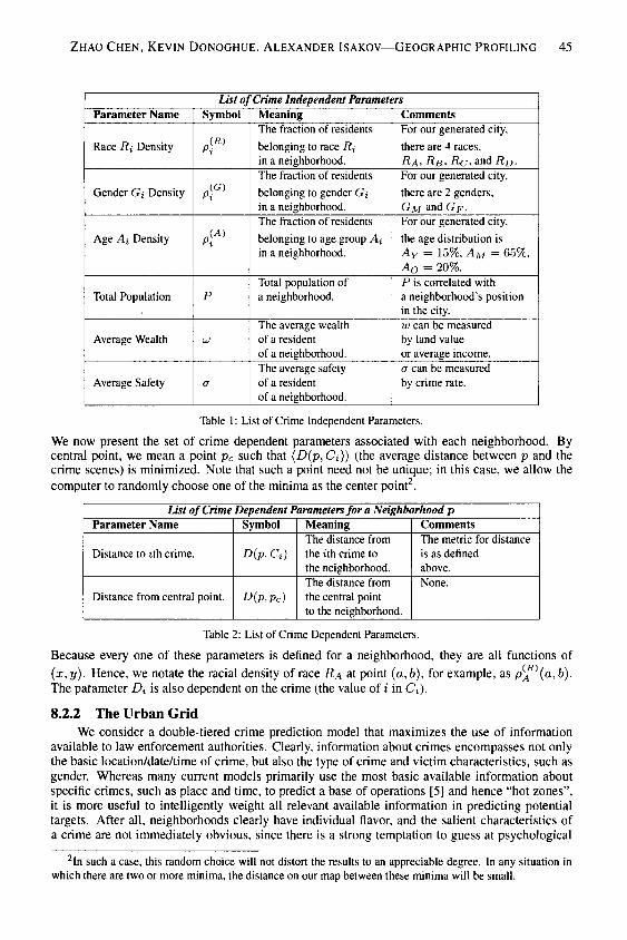
Zhao Chen, Kevin Donoghue, Alexander Isakov—Geographic Profiling 45
List of Crime Independent ParametersParameter Name Symbol Meaning Comments
Race Ri Density A*The fraction of residentsbelonging to race Riin a neighborhood.
For our generated city,there are 4 races,Ra, Rb, Rc^nd Rd-
Gender Gi Density Pr The fraction of residentsbelonging to gender Giin a neighborhood.
For our generated city,there are 2 genders,Gm and Gp-
Age Ai Density ^The fraction of residentsbelonging to age group Aiin a neighborhood.
For our generated city,the age distribution isAY = 15%, AM =65%,A0 = 20%.
Total Population pTotal population ofa neighborhood.
P is correlated witha neighborhood's positionin the city.
Average Wealth UJThe average wealthof a residentof a neighborhood.
w can be measuredby land valueor average income.
Average Safety (JThe average safetyof a residentof a neighborhood.
<j can be measuredby crime rate.
Table 1: List of Crime Independent Parameters.We now present the set of crime dependent parameters associated with each neighborhood. Bycentral point, we mean a point pc such that (D(p, Ci)) (the average distance between p and thecrime scenes) is minimized. Note that such a point need not be unique; in this case, we allow thecomputer to randomly choose one of the minima as the center point2.
List of Crime Dependent Parameters for a Neighborhood pParameter Name Symbol Meaning Comments
Distance to ilh crime. D ( p , d )The distance fromthe zth crime tothe neighborhood.
The metric for distanceis as definedabove.
Distance from central point. D(p,Pc)The distance fromthe central pointto the neighborhood.
None.
Table 2: List of Crime Dependent Parameters.Because every one of these parameters is defined for a neighborhood, they are all functions of(x, y). Hence, we notate the racial density of race Ra at point (a, b), for example, as p"A (a, b).The parameter Di is also dependent on the crime (the value of i in d).
8*2.2 The Urban GridWe consider a double-tiered crime prediction model that maximizes the use of information
available to law enforcement authorities. Clearly, information about crimes encompasses not onlythe basic location/date/time of crime, but also the type of crime and victim characteristics, such asgender. Whereas many current models primarily use the most basic available information aboutspecific crimes, such as place and time, to predict a base of operations [5] and hence "hot zones",it is more useful to intelligently weight all relevant available information in predicting potentialtargets. After all, neighborhoods clearly have individual flavor, and the salient characteristics ofa crime are not immediately obvious, since there is a strong temptation to guess at psychological
2In such a case, this random choice will not distort the results to an appreciable degree. In any situation inwhich there are two or more minima, the distance on our map between these minima will be small.

4 6 T h e H a r v a r d C o l l e g e M a t h e m a t i c s R e v i e w 3
motivation and use such guesses in predictions [10]. Insofar as we consider serial crimes [1] thatneither target specific individuals (as opposed to contract killings or political abductions) nor specific neighborhoods for their peculiar "local flavor", it is best to first strip the city of all except themost relevant factors that can lead to accurate predictions. We generate a city as follows.
1. Specify a grid size. We use a 10 x 10 grid, which allows for a wide mix of characteristicsto be dispersed through the city.
2. Specify P for each neighborhood. We assume that population is denser around easy-to-access places, so we choose from a uniform distribution based on distance from the line x —3. We have the population for each neighborhood drawn from [Unif(10,100—10(|_ — 3|))J,so that each neighborhood has at least 10 people.
3. Specify w and a for each neighborhood. These relative numbers will be useful in gauging a criminal's psychological parameter. We suppose that on average wealthier and saferneighborhoods are farther from the city center, a, u> are drawn from [Unif(l, 2 4- l/2(|x -4| + .J2/ — 4|))J, which will avoid unreasonable disparities in wealth and safety.
4. Input transporation. Adjacent points connected by fast transportation are counted as onlyI units of distance apart. This is important since serial criminals often take transportationinto account when they plan their actions [1,2].
5. Assign demographic information to each person. For each person in a neighborhood i, weassign a race, gender, and age. At the onset, only the age types are not equally distributed,but we will later modify racial distributions to test our model in circumstances where race isan issue.
Our model of a city as a grid has some important features that bear mentioning. For one, notethat all parameters are chosen independently of each other. Also, all parameters (including wealth)are discrete for faster coding and to represent the easily avilable information (it is easier and oftenmore useful to classify someone as "middle class" rather than assigning a real number to his or herwealth). Certain parameters are specific to the individual (e.g. race), while some are specific to aneighborhood (e.g. wealth).
8.2.3 Calculating Probabilities and Weights on the Urban Grid
Suppose that we have the crime vectors £1,..., £n- We need at least n = 5 crime incidentsin a serial case, which is a threshold for useful geographic profiling [4]. We assume that everyneighborhood on our grid has either zero population data or an appreciable population size, whichallows us to use densities rather than absolute numbers (e.g. using p\ ' rather than the total numberof residents of race Ri) to draw conclusions.
In terms of criminal characteristics, we suppose that the criminal is attacking strangers, consistent with many criminology studies [1]. Serial criminals who attack known associates are muchless prone to victim selection patterns, and hence the sporadic nature of their attacks are not suitable for geographic profiling. We assume that the criminal is acting on his own, and his actionsare apolitical and not associated with any organization (legal or otherwise). Further, we assumethat parameters in the psychological map are independent of one another as viewed by the criminal. Although it is also reasonable to suppose that serial criminals are generally aware of theirsurroundings, or at least have some working knowledge of the makeup of the nearby environment,our model nonetheless takes the possibility of random action seriously by subtracting the consistentcharacteristics of victims from the overall relevant population characteristic averages to account forthe "state of readiness" to commit a crime [1].
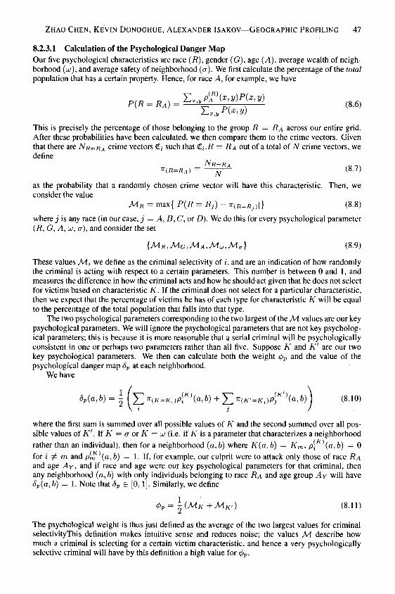
Zhao Chen, Kevin Donoghue, Alexander Isakov—Geographic Profiling 47
8.2.3.1 Calculation of the Psychological Danger MapOur five psychological characteristics are race (R), gender (G), age (A), average wealth of neighborhood (oo), and average safety of neighborhood (a). We first calculate the percentage of the totalpopulation that has a certain property. Hence, for race A, for example, we have
p r / ? - R ^ - _ _ _ _ _ _ _ _ 1 < X Mp { r ~ R a ) - e , , p ( * , » ) ( 8 ' 6 )This is precisely the percentage of those belonging to the group R = Ra across our entire grid.After these probabilities have been calculated, we then compare them to the crime vectors. Giventhat there are Nr=ra crime vectors £j such that di.R = Ra out of a total of N crime vectors, wedefine
* ( R = R A ) = ^ - ^ ( 8 - 7 )
as the probability that a randomly chosen crime vector will have this characteristic. Then, weconsider the value
M r = m a x { | P ( i ? = R , ) - t t ( r = R j ) \ } ( 8 . 8 )where j is any race (in our case, j = A, B, C, or D). We do this for every psychological parameter(R, G, A, oo, a), and consider the set
{ M r , M g , M a , M u , M * } ( 8 . 9 )These values Mi we define as the criminal selectivity of i, and are an indication of how randomlythe criminal is acting with respect to a certain parameters. This number is between 0 and 1, andmeasures the difference in how the criminal acts and how he should act given that he does not selectfor victims based on characteristic K. If the criminal does not select for a particular characteristic,then we expect that the percentage of victims he has of each type for characteristic K will be equalto the percentage of the total population that falls into that type.
The two psychological parameters corresponding to the two largest of the M values are our keypsychological parameters. We will ignore the psychological parameters that are not key psychological parameters; this is because it is more reasonable that a serial criminal will be psychologicallyconsistent in one or perhaps two parameters rather than all five. Suppose K and K' are our twokey psychological parameters. We then can calculate both the weight <pp and the value of thepsychological danger map Sp at each neighborhood.
We have
5 r ( a M = \ \ £ * < , K = K i ) P ? \ a M + ^ ^ K > = K i ) p f \ a , b ) \ ( 8 . 1 0 )
where the first sum is summed over all possible values of K and the second summed over all possible values of K'. If K = a or K — uj (i.e. if K is a parameter that characterizes a neighborhoodrather than an individual), then for a neighborhood (a, b) where K(a, b) = Km, p\K\a, b) = 0for i t£ m and p^(a, b) = 1. If, for example, our culprit were to attack only those of race Raand age Ay, and if race and age were our key psychological parameters for that criminal, thenany neighborhood (a, b) with only individuals belonging to race Ra and age group Ay will haveSp(a, b) = 1. Note that 5P e [0,1). Similarly, we define
< I > p = \ ( M k + M k > ) ( 8 . H )
The psychological weight is thus just defined as the average of the two largest values for criminalselectivityThis definition makes intuitive sense and reduces noise; the values M describe howmuch a criminal is selecting for a certain victim characteristic, and hence a very psychologicallyselective criminal will have by this definition a high value for <pp.

48 The Harvard College Mathematics Review 3
8.2.3.2 Calculation of the Spatial Danger Map and Total Danger MapFor every point p = (a, b) on our grid, we can calculate
(D(p,d)) (8.12)the average distance between p and the crime coordinates d. The point pc such that this averageis at a minimum is known as the central point. If there is more than one possible value for pc, werandomly select one.
We now calculate the values of the spatial danger map. First, we assign a value to every point pon our grid based on its proximity to the crimes, weighted towards the later crimes (consistent withthe idea that serial criminals tend to spread out as they commit more crimes, and hence a crimecommitted later would tend to be closer to other later crimes [15]). Namely,
£(P) = £(i.irD(p,a) (8.13)
The 1.1 is our weight factor*. We normalize this quantity and form
S(P) E„(i- i)<P(p,CQmax{£} (8.14)
where by max{£} we mean the maximum value of £ for all points in our grid. Hence, we now havea value between 0 and 1 to describe the proximity of any point to our crime scenes, with weighttowards the later crimes.
Next, given all the values D(pc, C\) for every d, we can define the radius 1Z of crimes as theaverage of these values, and the radial variance V of crimes as the variance of this set of values.Then, for any point p = (a, b), we have that
Ss(p) = S(a,b) = - (Exp (D(p,pc)-K)22V
+ £(P) (8.15)
The first term is a Gaussian with variance V and mean K. Hence, the first term produces a valuebetween 0 and 1 describing how much the D(p,pc) deviates from 11. This contribution follows thetheory that many criminals operate out of a "home base" [9], and hence their crime scenes tend toorient themselves to be approximately the same distance from this home base4. The second termdescribes how far away a point is from the crime scenes in general, and follows the theory thatcrime scenes tend to radiate outwards [14], which means that points closer to later crimes are morelikely to be chosen as subsequent crime sites. With these two contributions, we can define Ss(p), avalue between 0 and 1, and the psychological danger of a point.
What remains is to calculate the weight (ps. Given ak x £ grid,
= Exp - 0 VVkl. (8.16)
The parameter 0 > 0 depends on qualities of the city. The larger the value for 0, the more sensitiveto variance the weight (ps becomes. Hence, we would expect 0 to be larger for locales that are morecrowded or for larger grids in general, where the criminal has a larger activity region to function in.For our 10 x 10 grid, we use 0 = 5, and in this case we have
= Exp (8.17)
3The weight factor 1.1 is large enough to substantially weight £ towards the later crimes, but not largeenough to completely wash out data from the older crimes.
4Note that in this case, distance doesn't mean that we would geometrically expect a circle, since there existsa line of fast transportation down x = 3.
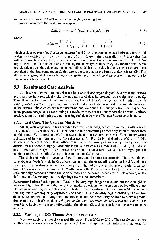
Zhao Chen, Kevin Donoghue, Alexander Isakov—Geographic Profiling 49
and hence a variance of 2 will result in the weight becoming 1/e.We can now form the total danger map as
A(a, b) = xP((Ps)Ss(a, b) + xP(<PP)6p(a, b) (8.18)
where
^ ) = ^ r ( i + e - ^ ) , - T T ^ ) ( 8 1 9 )which assigns to every (a, b) a value between 0 and 2. xp is recognizable as a logistics curve whichis slightly modified so that ^(0) = 0 and xp(l) = 1 (to 4 significant digits), k is a value thatwill determine how steep the xp function is, and for our present model we use the value k = 4. Weapply the xp function in order to ensure that significant weight values for (pp, <ps are amplified, whileless significant weight values are made negligible. With this model, higher values of (pi are moreprevalent in the final sum, and as (pi decreases, the function xp((pi) begins to drop off rapidly. Thisallows us to gauge differences between the spatial and psychological models with greater claritythan a purely linear model.
8.3 Results and Case AnalysisAs described above, our model takes both spatial and psychological data from the crimes,
and based on how statistically significant each set of data is, produces two weights (ps and (pp.Thus, there are four possible general cases, based on whether (ps and (pp are each high or low. Inlimiting cases where only (ps is high, our model produces a high danger value around the locationsof the crimes - these cases are less interesting and we omit a full analysis from this paper. Wehence present here results after running our model with two cases - one where the criminal's crimesproduce a high (pp and high <ps, and one using real data from the Thomas Sweatt arsonist case.8.3.1 Test Case: The Cunning Murderer
Mr. X, with vengeance in his heart due to perceived wrongs, decides to murder 30-40 year old(Am) males (Gm) of Race Ra- He feels comfortable committing crimes only small distances fromneighborhood X, at coordinate (6,6). However, he does not commit crimes at X, but rather withina distance of between one and two from that point. Ss (Fig. 2) is weighted by xp((ps) = 0.944,which is not too far from 1. It is farther from 1 since the crime pattern is not perfectly circularlydistributed but shows a highly symmetrical spatial cluster with a radius of 1.3. Sp (Fig. 3) alsohas a high overall weight of .751, since the criminal is consistent. We see that it highlights theneighborhoods with similar demographics to the intended targets.
The choice of weights makes A (Fig. 4) represent the situation correctly. There is a dangerzone about X (with X itself having a lower danger than the surrounding neighborhoods), and thereis a rapid drop in danger as we move away from the radius, due to the heavy spatial organization. This is a clear reflection of the "buffer zone effect", as explained in [13]; X is relativelysafe, but neighborhoods around the average radius of the crime scenes are very dangerous, with adeformation of symmetry due to weighting towards the later crimes.Recommendation: Station police officers in the very high danger zones and put those neighborhoods on high alert. Put neighborhood X on medium alert, but do not station a police officer there.Do not issue warning to neighborhoods outside of the immediate hot zone. Since Mr. X is bothspatially and psychologically organized, and hence has a reasonably high probability of targetingthe specific area without living there, the model should not necessarily be used to make a prediction as to the criminal's residence, despite the fact that the current models would put it at X. It ispossible to implement a search effort within the given radius, given that it is not overly expensiveto do so.
8.3.2 Washington DC: Thomas Sweatt Arson CaseNow we apply our model to a real-life case. From 2002 to 2004, Thomas Sweatt set fire
to 46 apartments and cars in Washington D.C. First, we split our city into four quadrants, for

5 0 T h e H a r v a r d C o l l e g e M a t h e m a t i c s R e v i e w 3
which we use available data on race distribution in Washington D.C. to give each quadrant theappropriate distribution in expectation. We assume that gender is uniformly distributed, and thatthe age distribution from a 2000 census is the same for all four quadrants. Then, we manuallyoverlay a 10 x 10 grid onto the city map and mark where the crimes were committed. We takecareful note of the Washington Post article on the subject, where there is a report that Thomas "toldinvestigators that he chose his targets at random" and that "he was acting largely on impulse whilescoping targets in a car" [17]. This suggests that Thomas was spatially organized (insofar as he didnot in general get very far from his place of residence before setting a fire) and not psychologicallyorganized, which we see from the random nature of 5P (Fig. 5), while Ss (Fig. 6) shows peakscentered at (7,4).
Since Washington D.C. is far from homogenous [19], the crimes seem to have some consistencyin them, which we see in Sp. However, these values are close to city averages, so the weight of thepsychological danger map is only .200, less than half the weight of the spatial danger map (.924).Putting the two together, we obtain a total danger map (Fig. 7) that is very consistent with Thomas'actual future crimes.Recommendation: Based on these ten crimes, we recommend heavily increased police presence inthe immediate hot zone (within a distance of roughly two neighborhoods of (7,4)). The heavy spatial organization as compared to the weak psychological organization suggests a residence searchstarting at a radius of .9 from the center point. A general community advisory is not suggestedoutside of the hot zone, since we see that the topography of the danger map is almost completelyflat compared to the peak.Comments on this Case: Considering the rest of the available crime data, we see that the modelworks incredibly well. The above recommendations would have helped prevent the next twocrimes, would have missed crime 13, 14, 165, and would have helped with crimes through 22,after which he started radiating outwards. However, we likewise note that once he started radiatingout, the heavy time weight of the later crimes compared to the early crimes would have made theradius calculation larger. However, Mr. Sweatt was actually located at (6,3)- right within the firstor second line of search. So, our geographical profiling model would have helped prevent the nextfew crimes that Thomas wanted to commit, and would ensure that he was caught at his place ofresidence before he could set the rest of the city on fire!
8.4 ConclusionAs seen in various test cases and in the above, our model generates useful predictions for
crimes that are not completely random. While we do not recommend that our model replace goodintuition and solid detective work, we have shown that it produces results that complements professional intuition in serial crime cases and helps direct search efforts and warn the inhabitantsof neighborhoods in imminent danger from a serial criminal without causing undue widespreadpanic. The 2005 case of the Washington D.C. arsonist Thomas Sweatt case is a perfect proof ofconcept. Using mild demographic assumptions informed by recent census data [19] and a manualgrid-overlay6, our model not only predicted the danger area of most of the subsequent offenses(given only the first 10 data points), but also accurately put the residence of Mr. Sweatt on thecorrect radius. In essence, the search space was limited to about five neighborhoods, which wouldhave facilitated Mr. Sweatt's arrest long before the rest of the string of arsons could unfold.
This outlines the general procedure for using the model and its advantages. A map of thecity, complete with necessary parameters, would be put on a grid and synchronized with policeinformation systems to automatically update. For a string of serial crimes, victim information andlocation would be put into the model, and after five or more data points7 were entered, the model
5Located at (6,6),(4, 5), and (6, 2), respectively.6Of course, accuracy would be greatly improved and the results would be even clearer in real life due to the
data and technology available to law enforcement that allows near-instantaneous localizations and data input ongrids.
7Fewer are possible, of course, but then the predictions will likely be rather inaccurate due to lack of data

Zhao Chen, Kevin Donoghue, Alexander Isakov—Geographic Profiling 51
would generate the recommendations similar to those outlined here. Any recommendation wouldbe used to either confirm or modify existing police efforts and community warnings, which wouldmake the city safer.
The dual-layered design of the model provides obvious advantages over the simple existingmodels. The calculations of (ps and (pp based on the crime data would allow one to automaticallyand intelligently place criminals on the gradient between selecting for victim location and selectingfor "victim type" (e.g. race, gender). The ability to make this distinction allows our profiling systemto go one step beyond pre-existing geographic profiling systems and deal with a more diversepool of serial crimes, saving resources and serving as a tool to pinpoint danger zones even if noprediction about criminal residence is appropriate.
For further research, we suggest that increased accuracy can be achieved if the nature of thecrime is considered. For example, we would expect gender to always be a strong factor in serialrape cases, but this factor does not give us much information about the psychological consistencyof the culprit; hence, it may be reasonable to omit the contribution from the gender parameter in thecalculation of (pp. Likewise, one could take a different account of parameters depending on the areain question. For example, gender may be weighted less in a city where it is too evenly distributedto be much help and would only add noise into the model. Practical spatial considerations, such asaccessibility due to roads or railways would impact the likelihood of a criminal being more spatiallythan psychologically motivated. The psychological equivalent to this, which would make the modelmore sophisticated, is the use of coupled parameters, i.e. if a culprit exclusively attacks citizens ofrace Rb and gender (7m, then those neighborhoods with high densities of citizens who are both ofrace Rb and male can be weighted more heavily as dangerous areas. We hope that further work onthis approach will provide a great ally for law enforcement.
References[1] PL. Brantingham, and P. J. Brantingham. Nodes, Paths and Edges: Considerations on the
Complexity of Crime arid the Physical Environment. J. Environmental Psychology. (1993) 13,3-28.
[2] P. L. Brantingham, and P. J. Brantingham. Notes on the Geometry of Crime. In PJ. Brantingham, and PL Brantingham. (eds.), Environmental Criminology, (1981) Sage Publications,Beverly Hills, 27-54.
[3] P. L. Brantingham, and P. J. Brantingham. Residential Burglary and Urban Form. (1975)Urban Studies. 12,273-284.
[4] D. Canter. Confusing Operational Predicaments and Cognitive Explorations: Comments onRossmo and Snook et al. Applied Cognitive Psychology. (2005) 19.5, 663-668.
[5] D. Canter, T. Coffey, M. Huntley, and C. Missen. Predicting Serial Killers' Home Base Usinga Decision Support System. J. Quantitative Criminology. (2000) 16, 457^178.
[6] J. E. Douglas, et al. Criminal Profiling from Crime Scene Analysis. Behavioral Sciences andthe Law. (1986)4.4,401-421.
[7] D. Jamieson. "Why Thomas Sweatt Set Washington on Fire." AlterNet. 8 June 2007. Accessed22 February 2010. http://www.alternet.org/story/53378/
[8] K. Fritzon. An Examination of the Relationship between Distance Travelled and MotivationalAspects of Arson. J. Environmental Psychology. (2000) 21, 45-60.
[9] R. N. Kocsis, and H.J. Irwin. An Analysis of Spatial Patterns in Serial Rape, Arson, and Burglary: The Utility of the Circle Theory of Environmental Range for Psychological Profiling.Psychiatry, Psychology and Law. (1996) 4.2, 195-206.
and the model would not be as useful.
5 2 T h e H a r v a r d C o l l e g e M a t h e m a t i c s R e v i e w 3
[10] D. J. Paulsen. Human Versus Machine: A Comparison of the Accuracy of Geographic Profiling Methods. J. Investigative Psychology and Offender Profiling. (2006) 3, 77-89.
[11] W. Petherick. Serial Crime: Theoretical and Practical Issues in Behavioral Profiling, Academic Press, Massachusetts, 2008.
[12] D. K. Rossmo. Place, Space, and Police Investigations: Hunting Serial Violent Criminals. InJ.E. Eck , and D.L. Weisburd. (eds.), Crime and place: Crime prevention studies, (1995) Vol.4, Criminal Justice Press, New York, 217-235.
[13] D.K. Rossmo. Geographic Profiling, CRC Press, Florida, 2000.
[14] B. Snook, et al. On the Complexity and Accuracy of Geographical Profiling Strategies. J.Quantitative Criminology. (2005) 21.1, 1-26.
[15] B. Snook, et al. Serial Murderers' Spatial Decisions: Factors that Influence Crime LocationChoice. J. Investigative Psychology and Offender Profiling. (2005) 2, 147-164.
[16] J. Warren, et al. Crime Scene and Distance Correlates of Serial Rape. J. of Quantitative Criminology. (1998) 14.1, 35-59.
[17] D. W. Wilber, and S. Horwitz. "Targets of Arson Picked Randomly, Investigators Say." Washington Post. 29 April 2005. Accessed 21 February 2010. http://www.washingtonpost.com/wp-dyn/content/article/2005/04/28/AR200504280 1403.html
[18] CBSNews.com CBS News, Associated Press, Prince George's County. Accessed 22 February2010. http://www.cbsnews.com/htdocs/fires/arson/mapJntro.html
[19] CensusScope: 2000 Census Data, Charts, Maps, and Rankings Social Science Data AnalysisNetwork. Accessed 22 February 2010. http://censusscope.org/

FEATURE9
MY FAVORITE PROBLEM
Sums of Four Squares
Tony Feng*Harvard University ' 13Cambridge, MA 02138
t feng@col lege.harvard .edu
Lucia Mocz*Harvard University '13Cambridge, MA 02138
lmocz@col lege.harvard.edu
9.1 IntroductionPick any natural number n. As the 18th-century mathematician Joseph Lagrange proved, you canalways write n as a sum of four perfect squares. Not impressed? Try to do the same for threesquares — you'll find that it is already impossible at 7. Think a greedy algorithm will work? Justtry 23. Still not impressed? Then read on to find out why this seemingly simple theorem makes itas this issue's My Favorite Problem.
We begin with a completely elementary proof by descent, a straightforward method exemplifying the apparent simplicity of elementary number theory. Armed with more machinery, we thenpresent solutions via Minkowski's theorem, lattices, and modular forms, demonstrating this theorem's intrinsic connection to modern techniques in algebraic and analytic number theory and geometry. These solutions highlight the beauty of elementary number theory. It is a subject concernedwith seemingly simple problems regarding the properties of numbers — integers in particular —with surprising connections and deep consequences for the rest of mathematics.
9.2 First Proof: Method of DescentIn this section, we give a completely elementary proof of the theorem by Fermat's classical methodof descent. First, we prove the following lemma.Lemma 1. Given a prime p, there exist a,b £ Z such that a2 + b2 + 1 = 0 (mod p).
Proof. Consider the equationa = — 1 — b (mod p).
There are (p+ l)/2 possible values for a2 and (p+-1)/2 possible values for -1 - b2, so they mustc o i n c i d e a t s o m e v a l u e , b y t h e p i g e o n h o l e p r i n c i p l e . □Theorem 2 (Lagrange). Every natural number can be written as the sum of four perfect squares.
Tony Feng is a a sophomore mathematics concentrator at Harvard. In terms of math, Tony is mainly incomplex analysis and number theory, but I also like philosophy, algorithms, fiction, and cooking desserts.
* Lucia Mocz '13 is a mathematics concentrator at Harvard with a secondary field in music. Her interest inmathematics is twofold: she is allured by the zen-like nature of topology and enticed by the clever problems innumber theory. In addition to being the Problems Editor of The HCMR, she was a problem-writer for HMMTand formerly competed in the Siemens and ISEF competitions, where her interest in mathematics developed.
53

5 4 T h e H a r v a r d C o l l e g e M a t h e m a t i c s R e v i e w 3
Proof. Note the identity
(a2 + b2 + c + d2)(w2 + £2 + y2 + 22) = (aw + bx + cy + dz)2+ (ax — bw — cz + dy) + (ai/ + bz — cw — dx) -h (az — by + ex — dw) .
This shows that the property of being a sum of four squares is closed under multiplication (thisidentity is motivated by the quaternionic norm). Therefore, it suffices to prove that every prime isa sum of four squares.
Now fix a prime p. By lemma 1, there exist integers x and y such that x2 4- y2 + 1 is divisibleby p. Thus, there exists a number ra such that mp may be expressed as the sum of the squares ofat most four integers:
m p = x \ + x \ + x l + x \ . ( * )We can consider ra < p as an additional constraint.1 We will show that if ra > 1, then ra can be"reduced"; that is to say, we can always find a smaller number n < ra such that np can also beexpressed as the sum of at most four squares.
We have two cases. Suppose first that ra is even. Then (*) is even, and we have three subcases: all four Xk (k = 1,2,3,4) are even, exactly two of the Xk are even, or all four Xk axe odd.In each case, the numbers can be paired such that each pair consists of two numbers with the sameparity. Without loss of generality, we pair x\ with x2 and £3 with X4. Then the numbers
(xi+x2)/2, (xi-x2)/2,
(x2 + xa)/2, (x3 -xa)/2,are integers. Thus
r a / £ i + # 2 \ 2 , / r X i - X 2 \ 2 , / X ' 3 + X 4 \ 2 , / r X 3 ~ X 4 \ 2- 2 - p = \ - ^ r ) + \ — r - ) + ( — 2 — ) + \ — r - ) ■
That is, (m/2)p can be expressed as the sum of the squares of at most four integers.Now consider ra to be odd. Let yk (k = 1,2,3,4) be the remainder smallest in absolute value
when Xk is divided by ra, i.e.:
xk = mqk + yk (k= 1, 2,3,4)
where yk can be either positive or negative and \yk\ < ra/2.We thus have
x\ = m2ql + 2mqkyk + yl = mQk + Vk (k = 1,2,3,4)
where Qk = rag2, + 2qkyk is an integer. Therefore,
rap = x\ + x\ + x\ + x\ = rag + y\ + y\ + y\ + 2/4where g = Qi -j- Q2 + Q3 + <?4, and
2/i + vl + J/3 + yi = mnwhere n = p — q. We also have n < ra since
mn = 2/? + 2/| + y\ + y| < 4(ra/2)2 = ra2
and moreover, n / 0, or else all the Xk would be divisible by ra and thus (*) would necessarily bedivisible by ra2, which is impossible since p is prime and ra ^ 1 and m < p.
!In the cited lemma, we can select a and 6 to be both less than p/2, that is, so that the sum a2 + b2 +■ 1 isless than p2 and therefore the quotient m resulting from dividing x2 +■ y2 +- 1 by p will be less than p.

Tony Feng and Luc ia Mocz—Sums o f Four Squares 55
We now want to show that np can also be expressed as the sum of not more than four squares.Use the identity cited at the beginning of this solution once more to show that the product mp-mn =m2np may be expressed as the sum of the squares of four numbers (since ran and rap are each thesum of four squares):
m2np = (xiyi + x2y2 + x3y3 4- rr42/4)2+
(xiy2-x2yi -\-x3y4-x4y3)2 4- (xiy3-x3yi +x4y2-x2y4)2 4- (xiy4-x4yi -\-x2y3-x3y2)2.We show that both sides of this equality are divisible by in2. Since Xk = rag/c4-2/fc, each expressionin the parentheses on the right side of the equality is divisible by ra. Furthermore, in the first set ofparentheses, we have that 2/1+2/2 + 2/3+2/4 — win, which is divisible by ra, and in the remainingthree sets, all products of the form yiyj cancel. Dividing both sides by rn2, we get
2 2 2 2np = zx 4- z2 4- z3 4- z4,
as desired.Therefore, if ra in (*) is not equal to 1, it can always be decreased, i.e., there will always be a
positive n < ra such that a similar equality exists. If n ^ 1, we can decrease n further. Thus wecan always find a sequence of positive integers ra > n > ni > n2 > ... until we have for naturalnumbers Xk (k = 1, 2,3,4) that
p = x2i+xl + xl + xl
9.3 Second Proof: Geometry of NumbersThe geometry of numbers has a close relation with other fields of mathematics, and an especiallyinteresting one with number theory. Informally, it is the study of convex bodies and integer vectorsin n-dimensional space. To understand its connection to this particular problem in number theory,we first develop a little machinery.
A lattice in a finite-dimensional euclidean space Rn is a discrete abelian subgroup that spansRn; it turns out a lattice in Rn is necessarily free of rank n.
Now let L C Rn be a lattice. Let A be a fundamental domain for L, i.e., the smallest areabounded by points in the lattice. If L is the group generated by vi,..., vn G Rn, then we could, forexample, take A = {tivi 4 f- tnvn,U G [0,1), Vz}. Then this set has the property that thetranslates of A by elements of L cover the plane and do not overlap. We denote by p the Lebesguemeasure onRn.Theorem 3 (Minkowski). Let K C Rn be a convex region symmetric about the origin with
p (K )>2nfi (A ) .
Then K contains a lattice point of L other than the origin.
Proof. We first show that the translates of \ K by the elements of L are not all disjoint. If we showthis, then we will be done. Indeed, we will then have found pi,p2 G \K and £1 ^ £2 G L suchthat
Pi +^1 =P2 + ^2,
which givese l - t 2 = P 2 - p i e K ( 9 . 1 )
since p2 — pi G \K — \K c K, as K is convex and symmetric about the origin. Then (9.1) isalso a nonzero element of L, which is what we want.

56 The Harvard College Mathematics Review 3
So suppose the contrary. Then we have a set of disjoint-translates \ K + £ for £ e L. As aresult, the intersections A D (|K 4- £) are disjoint. If we take their measures (with p denoting thestandard Lebesgue measure), we find that
MA)>X)^(An(|A- + <))=X;M((A-<)ni/f)=/i(iA-) = ^(na contradiction. Here we are using the fact that the Lebesgue measure p is translation-invariant andadditive for disjoint sets, as well as the fact that the sets A — £,£ e L cover R2. □
The proof of Lagrange's theorem is now a straightforward application of Minkowski's theoremand Lemma 1. The key idea to the following solution is a clever selection of our lattice to showthat each prime number can be written as a sum of four squares, i.e., p = a2 4- b2 4- c2 4- d2, where(a, b, c, d) is a point in our lattice.Proof. (Lagrange's theorem). Fix a prime p. By the previous lemma, we may pick a, b such that
a24-62 + l = 0 (modp).
Consider the lattice
where
L = {aiui 4- a2v2 4- 03^3 + a4^4 I a* G .
vi = (p, 0,0,0),i* = (0,p,0,0),V3 = (a, b, 1,0),V4 = (-6, a, 0,1).
The volume of the fundamental parallelogram is
p(A) = detp 0 0 0 ^0 p 0 0a b 1 0- b a 0 1 )
= P2.
Let K be a four-dimensional sphere around the origin with radius y/2p,
K = {(xi,x2,x3,X4) G R I Xi +x2 +x3 +x4 < 2p}.
Then p(K) = ^7r2(v/2p)4 = 2p27r2 > 2V(A). By Minkowski's theorem, K contains a nonzerolattice point (ui, u2,U3,U4) G L. Furthermore, we must have
0 < u\ 4- u\ + u2 + u\ < 2p.
Since this is an element of the lattice, we may write
(ui,u2,u3,U4) — ai^i +a2v2 4-03^3 + 04^4.
Thenu\ 4- U2 + ul + ^4 = a2(a2 + 62 4- 1) + a2(a2 + 62 4- 1) = 0 (mod p).
So we must actually have u\ + u\ 4- u! + u2 = p.

Tony Feng and Luc ia Mocz—Sums o f Four Squares 57
9.4 Third Proof: Modular FormsModular forms play a central role in modern number theory. Briefly put, they are a class of veryspecial functions that generalizes the notion of periodic functions. For brevity, we will have to takesome facts on faith in this section.
Let T be the modular group SL2(Z). For any finite-index subgroup V of T, we make thefollowing definition.Definition 4. A complex function / is called a modular form of weight k for T' if
• / is holomorphic in the upper half-plane HI.
-(: J)^.• For 7 = ( „ w ) € T', we have:
f(fz) = (cz + d)kf(z)
where 7 acts on z by Mobius transformation.
• / is holomorphic at the "cusps" in some sense.
The second condition is the, key symmetry property of modular forms. Note that as a specialcase, it implies f(z) is periodic, and the third condition is a technical point about the resultingFourier series of /.
Clearly, the constant functions are trivial examples of modular forms. It is not at all obviousthat nontrivial modular forms even exist, and indeed this is the point: the symmetry properties ofmodular forms (of weight k) are so special that they form a finite-dimensional vector space. Wewill not prove this fact here, but it is a standard result in many references (e.g. [1]).
Proof. (Lagrange's theorem). Let r4(n) = #{(a, b, c, d) G Z4 \ a2 + b2 4- c2 4- d2 = n}, i.e. thenumber of quadruples of integers whose squares add up to n. Let
00
— OO
Then 0(g)4 is precisely the generating function for r4(n). Moreover, one can show that
0(g)4 is a modular form of weight 2 and level 4.
Here "level 4" refers to the precise subgroup r'cT with respect to which 0(g)4 is a modularform. We also have the following fact:
The space of modular forms of weight 2 and level 4 is a 2-dimensional vector space.
It turns out that
J2 (sJ2d-32 J2d)qnn > 0 \ d \ n 4 d \ n J
is also a modular form of weight 2 and level 4. Therefore, we can verify that the two functions areactually equal by checking the first few terms of their Fourier expansions. This gives an explicitformula: r4(n) = 8 J2d\n d ~ 32 I^4d|n d, which is clearly positive. □

58 The Harvard Col lege Mathemat ics Review 3
9.5 ConclusionLagrange's theorem has even further consequences in the evolution of number theory. Additionalsolutions exist using Hurwitz quaternions, Aubry's lemma, and a combination of Ramanujan'sbilateral formula and Jacobi's triple product identity. There even exists a randomized polynomial-time algorithm (running in O(log(n)2) time!) for computing a representation n = a24-&2+c2+d2for a given integer n.
But given such a representation, is it unique? No, for we immediately see that
4 = l2 4-12 + l2 + l2 = 22 4- 02 4- 02 4- 02.
We next ask the natural question of just how many ways we can write a number as the sum of foursquares. In fact, Jacobi proved a much stronger result of Lagrange's theorem, that the number ofways in which a positive integer can be so written equals 8 times the sum of its divisors that are notmultiples of 4 (can you see why Lagrange's theorem follows from this as a direct corollary?). Weencourage the enthusiastic reader to find further generalizations of this problem and to explore itswide set of solutions.
References[1] F. Diamond and J. Shurman. A First Course in Modular Forms. Springer, 2005.
[2] S. Lang. Algebraic Number Theory. Springer-Verlag, 1994.[3] A. Lozano-Robledo. Untitled seminar notes on Minkowski's theorem. Available at http:
//math.bu.edu/people/alozano/seminar/minkowski.pdf.

FEATURE— 10 —Problems
The HCMR welcomes submissions of original problems in any fields of mathematics,as well as solutions to previously proposed problems. Proposers should direct problems to hcmr-problems@hcs . harvard, edu or to the address on the inside frontcover. A complete solution or a detailed sketch of the solution should be included, ifknown. Unsolved problems will not be accepted. Solutions to previous problems shouldbe directed to hcmr-solut ions@hcs . harvard. edu or to the address on the insidefront cover. Solutions should include the problem reference number, the solver's name,contact information, and affiliated institution. Additional information, such as generalizations or relevant bibliographical references, is also welcome. Correct solutions willbe acknowledged in future issues, and the most outstanding solutions received will bepublished. To be considered for publication, solutions to the problems below should bepostmarked no later than December 24, 2011. We encourage all submitters to typesettheir submissions in I#TeX and submit the source code along with the pdf.
All - 1. Let a, b, c be positive real numbers. Prove that:
6(ab 4- be 4- ac)Va3 + b3 y/b3 + c3 y/c3 4- a3a2 + b2 + b2 + c2 + c2 + a2 ~ (a + & + c)^(a4.&)(& + c)(c4-a)
Proposed by Tuan Le (Fairmont High School, Anaheim, CA)All - 2. Are there any simple groups of order p(p 4- 1), where p is prime?
Proposed by Eric Larson '13.
All-3. Let£ = {M G Mat3x3(R) : tr(M) = 0 and 4(^(M*))3 + 27(det(M))2 > 0} whereM* is the adjugate matrix of M. Let A,B G E such that A and B have no common eigenvectors.Suppose
(Bei,e3)(Be2,ei)(Be3,e2) = (Bei,e2)(Be2,ei)(Be3,ei)where (,) denotes the inner product and (ei,e2,e3) is the canonical basis of R3. Suppose as wellthat
Ani Bqi An'2 Bq2 • • -AnkBqk =1where n*, qi G Z. Prove that
A-niB'qiA~n2B'q2-' .A~nkB~qk =1
Proposed by Moubinool Omarjee (Paris, France).All - 4. Let x, y, z be three positive real numbers such that x 4- y + z = xyz. Prove that
3^ Vx^Tl ~ t^ X2 + 1 ^ J(X2 + 1)^2 +
<l)(2/2 + l) -2e y e Y e y e e y e
Proposed by Cezar Lupu (University of Bucharest, Bucharest, Romania).All - 5. Let a G N* be a fixed integer. Prove that there are an infinity of positive integers ra suchthat cr(ara) < cr(am 4-1) where a(n) is the sum of the divisors of the positive integer n.
Proposed by Vlad Matei (University of Bucharest, Bucharest, Romania).
59

6 0 T h e H a r v a r d C o l l e g e M a t h e m a t i c s R e v i e w 3
All - 6. Consider the set S of all strings over an alphabet of three symbols. Give it a groupstructure where the law of composition is concatenation and each word w in the group satisfies therelation ww = 1. Compute the structure of the group and show that although it is finite there existsan infinite string with no substring of the form ww, where w is a word.Note. There is an interesting generalization of this problem by replacing the relation w2 = 1 with higherpowers. We encourage the interested reader to submit his or her solution to this generalization as well.
Proposed by Lucia Mocz ' 13 and Dmitry Vaintrob '11.
Editor's Note: The following problem from the previous issue is released again as itreceived no solutions.
S08 - 2. Professor Perplex is at it again! This time, he has gathered his n > 0 combinatorialelectrical engineering students and proposed:
"I have prepared a collection of r > 0 identical and indistinguishable rooms, each ofwhich is empty except for s > 0 switches all initially set to the 'off' position. Youwill be let into the rooms at random, in such a fashion that no two students occupy thesame room at the same time and every student will visit each room arbitrarily manytimes. Once one of you is inside a room, he or she may toggle any of the s switchesbefore leaving. This process will continue until some student chooses to assert thatall the students have visited all the rooms at least v > 0 times each. If this studentis right, then there will be no final exam this semester. Otherwise, I will assign aweek-long final exam on the history of the light switch."
What is the minimal value of s (as a function of n, r, and v) for which the students canguarantee that they will not have to take an exam?
Proposed by Scott D. Kominers '09/AM' 10/PhD' 11, Paul Kominers (MIT ' 12), and Justin Chen(Caltech '09).

FEATURE" 11 -
Solutions
All Things Being Inequalities
S08 - 4. Consider a, b, c three arbitrary positive real numbers. Prove that
Ev/^ £,/db ..1 + fc±»-*+«>-8*h + C) V 4£cyca(a + &)(a + C)
Proposed by Cosmin Pohoata (Bucharest, Romania).Solution by Greg Yang 914. Note that if J2 appears without subscript, it will denote a sum overall symmetric variants of the polynomial that follows. For example, ]T ab = ab-\- bc-\- ca while^2 a2b — a2b+a2c+b2a+b2c+c2a+c2b. Explicitly, if the monomial that follows has 3 differentexponents, then there are 6 terms in the sum; otherwise there are 3 terms in the sum. Similarly forf| without subscript.
We will replace the 4 Y cyc «(a + b)(a + c) with 3 J2cyc a(a + )(a + c)t0 prove a strongerversion of the problem statement. Manipulate the inequality into the following form:
Scyc V H~ \z2cycy-bh) f (a + b)(b 4- c)(c 4- a) - Sabc2 £ « E < * V 3 £ e y e a ( a + W « ' + C )
Let f(x) = x~1^2. f is convex for x > 0. By weighted Jensen, the LHS is
Ecyc(& + «)/((« + b)c) / Ecyc(& + «)^\ _ / 2 £ aE f l + i * \ 2 £ a y y E a ^ + e n a '
On the other hand, let g(x) = x1/2. g is concave for x > 0. Again by weighted Jensen,
^cyc y b+Z ) Ecyc a9 \ (c+b)a )E a £ «
,Ecyc(^)T, /Ecyc 4fc T,cyda + b)(b + C)~9{ E« j V E« V (E")(n(« + »))/ E«2 + 3E«fe' (E«)(n(«+&))'
Hence it suffices to prove
2£a > / Ea2 + 3E«^ i^ + (a + fc)(fc + c)(c + a) - 8o6cEo2& + 6ria- V(Ea)(n(a + &))V 3EBta(fl + 6)(a + c)
61

6 2 T h e H a r v a r d C o l l e g e M a t h e m a t i c s R e v i e w 3
Since
3 2 a(a+b)(a+c)+II(a+b>) ~Sabc=3 (Ya3+Y °*h+3abc)eye
4- (J2a2b + 2a6c) ~ 8afec= 3 (]T a3 4- ]T a ) + (Y a2*> + 3a&c)
= (E")(3Ea2 + £<4(note that factorability here is the reason we replaced the 4 with the 3), we have
(2Ea) (Il(a + fo)) (3Ea(a + b)(a + c))>(E«2&+6n (Ea2+3E«b)(3E°2+E«6)-
Now we painfully expand. The easiest way is to note that the expansion is a 7-degree polynomialand then count the coefficient of each 7-degree monomial on each side. After expansion we get
3 ^ a 6 6 + 5 ^ a V + 5 ^ a 4 6 3 - 2 ^ a 5 6 c - 1 4 ^ a V c - 2 ^ a 3 6 3 c + 2 ^ a 2 6 2 c 3 > 0 .But we have by AM-GM
l-a3b3c+2-a«c>a%c =» ? ^aVc+?^a6c > 2^a56c (11.1)
±a2b2c3+l-c%2>c%2a => ^a262c3 + ^c562>^c462a (11.2)
la3b3c+±a6c>a4b2c =» ^a3b3c+ l^aec > X>Vc. (11.3)
Using one of (11.1) and (11.3) and two of (11.2), the inequality simplifies to
2 ^ a 6 6 + 4 ^ a V + 5 ^ a 4 6 3 - ^ l l a V c > 0 .Now this inequality is true by Muirhead as (6,1,0), (5,2,0), (4,3,0) all majorize (4,2,1). □
Cruel Mistress Induction
F08 -1. Let p, q be two positive integers, and let n be integers such that n > p 4- q. Prove that thefollowing identity holds:
S(:)(p!,)(;:;)=e0(-)(",-'Proposed by Cosmin Pohoata (Bucharest, Romania).
Solution by Arnav Tripathy '11. The right-hand side is
y[ P j fn\ fn - q \ = fn\ (n -q + pMp-vW\ { ) W\ pwhere the last step follows from noting that after factoring out a (") we are, in effect, just countingthe number of ways to choose p people from n — q males and p females in two different ways.

L u c i a M o c z , e d . — S o l u t i o n s 6 3
Hence, the problem follows by substituting r = n + p (and replacing i with p — i) in the followingclaim: for any r > p + q,
p\ I q\ I r — i \ _ I r — p\ I r — qY, , , , , , .^oW\V\p+9/ V q J V pwhich is in turn the special case d = 0 of the following more general claim: for any 0 < d <p, r > p 4- g — d, we have
y"(p\(q\( r~{ \ = Vi^\[rJri~p\(r~q\£<\i)\i)\p + q-d) ^J^-d + jJ^-j)
Indeed, denote the left- and right-hand sides above by f(p,q,r,d) and g(p,q,r,d), respectively. We prove that f(p,q,r,d) — g(p,q,r,d) by simultaneous induction on r and reverseinduction on d. In other words, we first note that the identity holds for r as small as possible, i.e.r — p-\-q — d, where f(p, q, r, d) = g(p, q, r, d) — 1, and for das large as possible, i.e. for d — p,where we have
i = 0 \ / \ / \ ^ / i = o \ / v / \ /
as desired.We finish by noting that
f(p, q, r, d) = f(p, q, r - 1, d) 4- f(p, q, r - 1, d + 1)
and
g(p, q, r, d) = g(p, q,r-l,d)-\- g(p, q,r-l,d+l)
so that the induction step follows. Indeed, using Ah(r) to denote h(r + 1) - h(r), we have
= f (p ,q , r,d+ 1 )
= y ^ / d \ / / r + d - . ? ' - p \ / r - q \ / r + d - j - p + l \ / r - q \ \f ^ 0 V ' \ S q - j - 1 ' { p - d + j ) V q - j ) \ p - d + j - i ) j
= g(p,q,r,d+ 1)
as claimed.
Also solved by Greg Yang '14

6 4 T h e H a r v a r d C o l l e g e M a t h e m a t i c s R e v i e w 3
Editor's Note: The following problem required a correction from the previous issue. Asolution by the editor is presented for the corrected problem.
Fun with Fermat
F08 - 2. Let p be an odd prime. For every positive integer n, let
A(n) = ln + 2n + --. + (p-2)n and B(n) = ln .+ (p - l)n.Let {ai} i be the sequence defined by ai — 2, a2 = p2 4- 2 and
an+2 = A(n)an+i 4- B(n)an ifp - 1 \ n,an+2 = [A(n) + B(n)]an+i + an if p - 1 | n.
Prove that no an is equal to the product of any p - 1 terms of the sequence {ai} i.
Proposed by Daniel Campos Salas (Costa Rica).Solution by Lucia Mocz '13. In this proof, we rely heavily on the result of the following theorem:Fermat's Little Theorem. If p is a prime number, then for any a e Z, ap — a is evenly divisibleby p. In modular notation, this can be stated as aP = a mod p. A variant to this statement is thatif a e Z is coprime to p then op_1 - 1 is evenly divisible by p. Again, in modular notation, wewrite this as a?~l = 1 mod p.
By this theorem, if we show that each term in the sequence is congruent to 2 modulo p, thenthe product of any p - 1 terms is congruent to 1 modulo p. It follows that as the product of anyp - 1 terms in the sequence is not congruent modulo p to any an, no an can be equal to the productof any p — 1 terms of the sequence.
We thus proceed by induction on n to show that all terms of the sequence are congruent to 2modulo p. We already have this is true for n = 1 and n = 2. Assume it holds for n and n 4-1. Wewant to show it also holds for n + 2. Then we have the following two cases:
1. First suppose that p - 1 \ n. Then we have
an+2 = A(ri)an+i 4- B(n)an = 2(A(n) 4- B(n)) mod pWe want to show that A(n) 4- B(n) = 1 mod p. From the previous calculation, we know
A(n) + B(n) = 1 4- (ln + 2n 4-... + (p - 2)n + (p - l)n) = 1 + x mod pNote that since Z/pZ is a field, then (Z/pZ)x (i.e., its group of units) is cyclic and acts onZ/pZ. Let (g) — (Z/pZ)x, where g generates the group. Then:
gn.x = gn + (2g)n + ... + (g(p-l))n=x mod p
It follows that x(gn — 1) = 0 mod p. However, since p - 1 \ n, we must have gn ^ 1mod p, which implies that x = 0 mod p. We are thus left with A(n) 4- B(n) = 1 mod p asdesired.
2. Now suppose that p — l|n. Then we have
an+2 = (A(n) + B(n))an+i + an = 2(A(n) + B(n)) 4- 2 mod pWe want to show that A(n) 4- B(n) = 0 mod p. We have, as in the previous case:
A(n) + B(n) = 1 4- (ln + 2n 4-... + (p - 2)n 4- (p - l)n) = 1 + x mod p

L u c i a M o c z , e d . — S o l u t i o n s 6 5
Since p - l|n, by Fermat's Little theorem, we have:
x = (lk)p~l 4- (2kY~l + ... 4- ((p - l)fc)p_1 = p - 1 mod p
where k — -^y. We are thus left with A(n) 4- B(n) = 1 + (p — 1) = 0 mod p asd e s i r e d . □
On a Rolle
F08 - 3. Let / : [0,1] -+ R be a differentiable function with continuous derivative such that
/ f(x) dx = / xf(x) dx.J o J o
Prove that there exists £ G (0,1) such that
/(0 = /'(O f f(*)dx.Jo
Proposed by Cezar Lupu (University of Bucharest, Bucharest, Romania).Solution by Paolo Perfetti (Dipartimento di Matematica, Universita degli di Tor Vergata Roma,Italy). If f = 0 there is nothing to prove, so we suppose / ^ 0. Define F(x) = fQx f(y)dy andobserve that
f F(x)dx = [ dx [ f(y)dy = [ dyf(y) e\ dx = f dyf(y)(l - y) = 0J o J o J o J o J oWe claim the set of points of [0,1], say iV, where F(x) — 0, is not dense on [0,1]. For otherwisewe would have F(x) = 0 on a dense set in [0,1] and then F(x) = 0 by continuity of F(x), butthis is forbidden by / ^ 0 via the continuity of f(x).
As a consequence, there exists an open interval (a, b) C [0,1] where F(x) ^ 0. Now define:
g : [ 0 , l ] \ N ^ R
g(x) = f(x)-ln\F(x)\We affirm that there exists the point x\ G [0, a], nearest to x = a, such that lim + g(x) = -hooand a point x2 G [b, 1], nearest to x = b, such that lima._>x- g(x) — -hoc (this is proved in amoment). By continuity of g(x) in the interval (x\ ,x2), for any y = y0 large enough there are twopoints vi and v2 both in (xi,x2) such that g(vi) = g(v2). Rolle's theorem tells us that g'(£) = 0at a point £ G (vi,v2) yielding
or
/(0 = /'(0 ff(x)dx.Jo
the existence of xi. Let A = {x e [0, a] : F(x) = 0}. A is nonempty since F(0) = 0 andbounded and then there exists sup A which is attained (is a maximum) since F(x) is continuous.The proof of existence of x2 is quite similar, but notice that it is essential J1 F(x)dx = 0 becauseotherwise the set of points B = {x e [b, 1] : F(x) = 0} might be empty. □Also solved by Arnav Tripathy ' 11

6 6 T h e H a r v a r d C o l l e g e M a t h e m a t i c s R e v i e w 3
Oh, the Choices You'll Make
F08 - 4. Do there exist functions /, g : R -+ R such that
• both are periodic, i.e. there exist nonzero real a, b such that for all x G R, f(x) = f(x 4- a)and g(x) = g(x 4- b), and
• their sum is equal to the identity, i.e. for all x G R, /(x) 4- #(#) = x?
Proposed by Robert Obryk (August Witkowski High School, Krakow, Poland).
Solution by Oliver Knill (Harvard University). We can assume a = 1 by rescaling the axes. Wecan assume b irrational because for rational b = p/q the condition f(x) 4- g(x) = /(x 4- qb) 4-#(x 4- qb) = x 4- go collides with f(x) 4- #(#) = x. The condition /(x) 4- g(x) = x means
f(x 4- fc6 4- /) + g(x 4- fc& 4- /) = x 4- fc6 + /for all x and all integers k, I. By the a = 1 periodicity of / and the b periodicity of g, this is
f ( x + k b ) + g ( x + l ) = x + k b + l . ( 1 1 . 4 )
Define an equivalence relation on the reals by
x ~ y <=> x 4- kb 4- / = 2/ for some integers /c, /.
Let X be the quotient X = R/ ~. We can chose a member x(s) in each equivalence class of Xby the axiom of choice. Define f(x(s)) = x(s) and g(z(s)) = 0. Now the values of / and g oneach equivalence class is determined with
f(x(s) + kb) = f(x(s) 4- A:6 + /) = x(s) + kbg(x(s) + l) = g(x(s) + kb + l) = l
This defines the values of / and g for every x because every real x can be written as x = x(s) 4-/c6 + /, with s e X,k,l eZ. Adding these two equations gives (11.4). Note that the functions /, gare given in a nonconstructive way and non Lebesgue measurable but they do exist if one acceptst h e a x i o m o f c h o i c e . □Also solved by the Missouri State University Problem Solving Group and Arnav Tripathy ' 11
Three's a Charm
F08 - 5. Let ABC be an arbitrary triangle and let / be the incenter of ABC. Let D, E, F bethe points on lines BC, CA, AB respectively such that /.BID = AC IE = ZAIF = 90°, anddefine the following measurements: ra,n,rc are the exradii of the triangle ABC, A' is the areaof DEF, and A is the area of ABC. Prove that
A^ _ 4r(ra + rb 4- rc)A ~ (a + b + c)2 '
Proposed by Mehmet §ahin (Ankara, Turkey).Solution by Kee-WaiLau (Hong Kong, China). Let a = BC, b = CA, c = AB. Denote by rand s, respectively, the inradius and semiperimeter of triangle ABC. It is well-known that r = y.We have
AF = ^/sec(^/2) = rcsc(A/2)sec(^/2) = -^- = 2 (-) (£-) = -S i n / \ . \ S J \ Z / L A / s

L u c i a M o c z , e d . — S o l u t i o n s 6 7
and similarly CE = ab/s.Hence AE = AC - EC = b- ab/s = b(s - a)/s and the area of triangle AFE is:
(AF)(AE)sinA _ 1 (bc\ (b(s-a)\ /2A\ _ b(s - a)A2 2 V s J V s J V b e
Similarly, the area of triangle BDF and CED are c(s — b)A/s2 and a(s — c)A/s2. Thus
, _ b(s - a)A 4- c(s - b) A 4- a(s - c)A _ 2(ab + bc + ca) - (a2 + b2 +■ c2)~ s 2 ~ ( a 4 - 6 + c ) 2
It remains therefore to show that 4r(ra + rb + rc) = 2(ab + be 4- ca) — (a2 + b2 4- c2). Usingthe well-known results: _ A _ _A_ - ^_^ " a — , r b — T 5 r c —s — a s — b s — c
and Heron's formula for A, we see that:
, 4 A / A A A4 r ( r a + n + r c ) = — I \ +s \s — a s — b s — c,
_ 4A2 ((s - b)(s - c) + (s - c)(s - a) + (s - a)(s - b))s(s — a)(s — b)(s — c)
= (a - 6 4- c)(a + b-c) + (a + b- c)(-a + 6 + c) -h (-a 4-6 4- c)(a -b + c)= 2(a6 + be 4- ca) - (a2 + 62 4- c2)
as desired.Also solved by Arnav Tripathy ' 11

FEATURE12
ENDPAPER
The Three-Legged TheoremMichael J. HopkinstHarvard University
Cambridge, MA [email protected]
The summer after my senior year in high school, I had a job driving a truck for a small companyin Nebraska. I'd start every day in Fremont, pull orders, load a truck and drive it to Lincoln. There Iwould unload the truck, shoot the crap with the guys in the warehouse, re-load and head to CouncilBluffs. From Council Bluffs, I drove back to Fremont. It was a pretty good job if you like drivingaround in the country and shooting the crap with guys in warehouses. The only problem was that Ihad trouble staying awake behind the wheel.
I tried several strategies. My first was to yell "hey!" and point every time I saw a bale of hay.My father did this all the time on family trips and I thought maybe I was at last old enough to do itmyself. Evidently I wasn't.
My next idea was to insult the cows. There are a lot of them scattered around the Nebraskacountryside and mostly they just kind of stand there. I thought it would be really cool to have acow to go, "wtf?!" This worked pretty well. I could get really worked up yelling insults at cowsand it definitely kept me awake. I pulled into Lincoln the first time I tried it, pumped up and in agreat mood. In the middle of shooting the crap, one of the warehouse guys asked me why I was soexcited and so hoarse. I stalled a bit before coming up with, "big night."
This went on for a couple of weeks during which I got a lot of respect from the warehouseguys, but no reaction at all from the cows. I started to wonder why. I had two theories. The firstwas that cows are stupid and that they couldn't hear me from the road anyway. I quickly dismissedthat as ridiculous. A more realistic explanation, I reasoned, was that cows are incredibly chill andthat they are born nearly enlightened, with a natural understanding that the world is an illusion andlife is suffering. They probably felt pity for me. That seemed about right, but it pretty much killedmy strategy for staying awake. I felt too guilty. That, and the fact that serenely slipping past fieldsof bovine buddahs was way too zen to keep me awake.
I needed a new idea and there happened to be one in my lunch bag. It was the textbook for aclass in point set topology I had taken at UNO that spring. I decided to road test my understanding,starting from page one. Before each trip I'd read the statement of a theorem and then try and proveit on the road. For a while I was doing pretty well. Then I got to the Heine-Borel Theorem.
The Heine-Borel theorem is the one characterizing compact subsets of Euclidean space. It'snot that the proof is so hard, but you really have to be organized in your mind to come up with it.I wasn't. I got all the way to Lincoln without getting anywhere at all. The warehouse guys askedme why I was so distracted. All I could come up with was, "big night." I got back in the truck anddrove to Council Bluffs. Still nothing. When I finally got back to Fremont I had to peek. In theend, I drove all three legs of my trip without even coming up with a clue on where to start.
This was my first encounter with a "three-legged theorem." They are something pretty special:little theorems that aren't that hard, but require really clear thinking. You meet,them from time totime, and if you're lucky, you cannot get anywhere at all trying to prove them. That's when youlearn something. Now that you know what to look for, keep your eyes open. They are all over theplace.
t Michael Hopkins has a PhD from Northwestern University and a D. Phil from Oxford University. He taughtat Princeton, the University of Chicago and MIT before coming to Harvard in 2004.
68

JANE STREETW W W. I A N E S T R E E T. C O M
N e w Y o r kL o n d o n
h o n g K O N G