IASSNS-HEP-97/5, NSF-ITP-97-014, cond-mat/9701212

The Haldane-Rezayi Quantum Hall State and Conformal Field

Theory

V. Gurarie∗ and M. Flohr†

Institute for Advanced Study, Olden Lane, Princeton, N.J. 08540

C. Nayak‡

Institute for Theoretical Physics, University of California, Santa Barbara, CA, 93106-4030

(October 20, 2007)

Abstract

We propose field theories for the bulk and edge of a quantum Hall state in

the universality class of the Haldane-Rezayi wavefunction. The bulk theory is

associated with the c = −2 conformal field theory. The topological properties

of the state, such as the quasiparticle braiding statistics and ground state

degeneracy on a torus, may be deduced from this conformal field theory. The

10-fold degeneracy on a torus is explained by the existence of a logarithmic

operator in the c = −2 theory; this operator corresponds to a novel bulk

excitation in the quantum Hall state. We argue that the edge theory is the

c = 1 chiral Dirac fermion, which is related in a simple way to the c = −2

theory of the bulk. This theory is reformulated as a truncated version of a

∗Research supported by NSF grant DMS 9304580 gurarie@ias.edu

†Research supported by the Deutsche Forschungsgemeinschaft flohr@ias.edu

‡Research supported by NSF grant PHY94-07194 nayak@itp.ucsb.edu

1

doublet of Dirac fermions in which the SU(2) symmetry – which corresponds

to the spin-rotational symmetry of the quantum Hall system – is manifest

and non-local. We make predictions for the current-voltage characteristics for

transport through point contacts.

Typeset using REVTEX

2

I. INTRODUCTION

In 1987, Willet, et al. [1] discovered a fractional quantum Hall plateau with conductance

σxy = 52

e2

h. Shortly thereafter, Haldane and Rezayi [2] suggested

ΨHR = A(u1v2 − v1u2

(z1 − z2)2

u3v4 − v3u4

(z3 − z4)2. . .

) ∏i>j

(zi − zj)2 e

− 1

4`20

∑|zi|2

(1)

(A means antisymmetrization over all exchanges of electrons, ui, vi are respectively up and

down spin states of the ith electron, and `0 is the magnetic length) as a variational ansatz

for the incompressible state of electrons observed in this experiment.1 Despite the passage

of nearly 10 years, this proposal has been neither confirmed nor ruled out by experiment,

in large part because the theoretical understanding of this state is still primitive. In this

paper, we try to address this deficiency by proposing effective field theories of the bulk and

edge of a system of electrons with ground state given by (1).

Our faith in Laughlin’s wavefunctions for the principal odd-denominator states stems not

only from their large overlap with the exact ground state of small systems. Rather, their

success lies in the fact that they exhibit properties – ‘topological ordering’ [3,4] – which

are plausibly far more robust than the specifics of any trial wavefunction. The ‘topological

ordering’, which refers to the fractional statistics of quasiparticles [5,6] and off-diagonal long-

range-order of certain non-local order parameters [4], could be demonstrated for Laughlin’s

wavefunctions because the plasma analogy facilitates calculations with these wavefunctions.

The ‘topological ordering’ is summarized by the (abelian) Chern-Simons effective field the-

ories of the quantum Hall effect (see also [7–9]). The fractional statistics is the linchpin

of the theory and its most startling prediction, and, hopefully, will be confirmed some day

soon. The Chern-Simons effective field theory led, in turn, to a conformal field theoretic

1(1) is a wavefunction for electrons at ν = 1/2. It is assumed that at ν = 5/2 the lowest Landau

levels of both spins are filled and the appropriate analog of (1) in the second Landau level describes

the additional ν = 1/2.

3

description of the edge excitations [10]. Detailed predictions based on the edge theory have

recently been spectacularly confirmed [11–14]. Unfortunately, there is no plasma analogy for

the Haldane-Rezayi wavefunction, nor for a number of other proposed wavefunctions such

as the Pfaffian state. Consequently, the correct Chern-Simons theory of the quasiparticle

statistics and the conformal field theory of the edge excitations have remained elusive.

A way of skirting this obstacle was suggested by Moore and Read [15]. They observed

that the Laughlin state and a number of other quantum Hall effect wavefunctions, including

the Haldane-Rezayi state, could be interpreted as the conformal blocks of certain conformal

field theories. This observation gains great power in light of the equivalence, discovered

by Witten [16], between the states of a Chern-Simons theory and conformal blocks in an

associated conformal field theory. It is often the case that a quantum Hall state can be

reproduced by the conformal blocks of a conformal field theory. Since this conformal field

theory is equivalent to a Chern-Simons theory, it is very tempting to close the circle, following

Moore and Read, and conjecture that this Chern-Simons theory is the desired effective

theory of the bulk, which would be obtained by a direct calculation using brute force or

some generalization of the plasma analogy. This conjecture is true for states with abelian

statistics, such as the Laughlin states and their hierarchical descendents. A general argument

in favor of this premise was given in [17], where it was used to deduce the SO(2n) non-abelian

statistics of quasiholes in the Pfaffian state once the correspondence between this state and

the conformal blocks of the c = 12

+ 1 conformal field theory was demonstrated in some

detail. If correct, this conjecture implies that the conformal blocks are the preferred basis

of the quantum Hall wavefunctions since they make the quasiparticle statistics transparent.

It has been observed [15,18,19] that the Haldane-Rezayi state is a conformal block in the

c = −2 conformal field theory. Here, we derive some consequences of this fact. Among these

is the 10-fold degeneracy of the ground state on the torus. The ground state degeneracy on a

torus is not merely mathematical trivia. It is equal to the number of ‘topologically dictinct’

quasihole excitations – ie. that have inequivalent braiding properties (so, for instance, the

combination of any excitation with a bosonic excitation does not produce a topologically

4

distinct excitation) – which there are in the system. As we will explain, the 10-fold degener-

acy is a surpise, and is due to the existence of an excitation which cannot be found in other

proposed even-denominator quantum Hall states, such as the Pfaffian and (3, 3, 1) states.

The 10-fold degeneracy is due, in the c = −2 conformal field theory, to the existence of a

logarithmic operator [27]. We elucidate the structure of the c = −2 theory, with particu-

lar emphasis on the calculation of conformal blocks and on the logarithmic operator. The

former allow us to obtain the non-abelian statistics of the quasiholes.

In principle, it should be possible to use the Chern-Simons theory of the bulk to deduce

the conformal field theory of the edge excitations. However, a more direct approach is

possible. As can be explicitly shown for the Laughlin states [20] (see, also, the second

ref. in [10]), the states of the edge conformal field theory can be enumerated by direct

construction of the corresponding lowest Landau level wavefunctions which are the exact

zero-energy eigenstates of certain model Hamiltonians. Under mild asumptions about the

confining potential at the edge of the system, which gives these excitations non-zero energy,

the energy spectrum can be obtained as well. Milovanovic and Read [19] generalized this

construction to the Pfaffian, (3, 3, 1), and Haldane-Rezayi states. In the case of the Pfaffian

and (3, 3, 1) states, their construction led immediately to the correct edge theory. We propose

that the edge theory of the Haldane-Rezayi state is a theory of a chiral Dirac fermion, with

c = 1. This theory possesses a global SU(2) symmetry which becomes manifest when recast

as a truncated version of a c = 2 theory. The SU(2) symmetry – which is just the spin-

rotational symmetry, an approximate symmetry in GaAs with its small g factor and effective

mass – is unusual in that the local spin-densities do not have local commutation relations

(see, also, [40]). This indicates the impossibility of localizing spin at the edge which, we

argue, is supported by an analysis of the explicit wavefunctions. The relationship between

the c = −2 and c = 1 theories [28,34,40] – they have nearly the same states, spectra, and,

therefore, partition functions – is very natural in this context since these theories describe

the bulk and edge of the Haldane-Rezayi state.

Section II is a review of the relevant facts and standard lore regarding the Haldane-Rezayi

5

state. In section III we recapitulate, in order to make our exposition as self-contained as

possible, the conformal field theory approach to the bulk wavefunctions in the quantum Hall

effect. In section IV, we discuss the c = −2 conformal field theory and, in section V, we

apply it to study quasiparticles in the Haldane-Rezayi state. Section VI is devoted to the

relationship between the c = −2 and c = 1 conformal field theories. The edge theory of

the Haldane-Rezayi state is discussed in section VII and the physical consequences following

from the results of sections V and VII are discussed in section VIII. Parts of this paper

are rather technical. Readers who are uninterested in the subtleties and finer points of the

c = −2 and c = 1 conformal field theories but are interested in the observable consequences

which follow from them may wish to skip or merely skim sections III, IV, and VI.

II. THE HALDANE-REZAYI STATE

In this paper, we will be studying the zero-energy eigenstates of the Hamiltonian [2]

H = V1

∑i>j

δ′(zi − zj), (2)

where V1 > 0. While this is almost certainly not the Hamiltonian governing any experiment,

it has the advantage of tractability, and the properties which interest us are universal and

should be stable against perturbations. We have assumed that the Zeeman energy vanishes

so (2) is invariant under SU(2) spin rotations. In GaAs, the Zeeman energy is 160

of the

cyclotron energy, so SU(2) will be a reasonable approximate symmetry.

This Hamiltonian shares with other simple, short-range lowest Landau level Hamilto-

nians the property that not only the ground state, but also states with quasiholes and

edge excitations, have zero energy. This should not be troubling since the incompressibility

of the quantum Hall state depends upon the existence of a discontinuity in the chemical

potential. If quasiparticles have finite energy but quasiholes do not, there will be such a

discontinuity. For a more realistic interaction, both quasiholes and quasiparticles have finite

energy, but the discontinuity persists. Since they are annihilated by the Hamiltonian, the

6

multi-quasihole states are easier to enumerate, so in what follows, we will discuss them ex-

clusively; the properties of quasiparticles – though difficult to study directly – are trivially

related to those of quasiholes. The vanishing energy of the edge excitations should not be

a surprise, either. These have finite energy only if there is a confining potential at the edge

of the system, as there will be in any real 2D electron gas. As we discuss further below,

we will simply assume that, in the presence of a confining potential, the energy of an edge

excitation is proportional to its angular momentum. For these reasons, we will refer to the

state with no quasiholes and no edge excitations – the maximally compressed state – as ‘the

ground state’ and refer to the other zero-energy states as ‘quasihole states’ and ‘edge states’,

respectively, despite the fact that, strictly speaking, all of these states are ground states of

(2). The multi-quasihole states, which are bulk excitations, can be distinguished from the

edge states by the property that the former must be homogeneous in the zi’s since only such

wavefunctions can be extended to the sphere (where there is no edge and, hence, no edge

excitations). The inhomogeneous zero-energy wavefunctions are edge states.

As we mentioned above, the ground state of (2) is the Haldane-Rezayi state,

ΨHR = Pf

(uivj − viuj

(zi − zj)2

) ∏i>j

(zi − zj)2 e

− 1

4`20

∑|zi|2

(3)

where Pf, the Pfaffian, is the square root of the determinant of an anti-symmmetric matrix,

or, equivalently, the antisymmetrized product over pairs introduced in (1). It resembles its

cousins, the ‘Pfaffian’ and (3, 3, 1) states:

ΨPf = Pf

(uiuj

zi − zj

) ∏i>j

(zi − zj)2 e

− 1

4`20

∑|zi|2

(4)

Ψ(3,3,1) = Pf

(uivj + viuj

zi − zj

) ∏i>j

(zi − zj)2 e

− 1

4`20

∑|zi|2

(5)

The Pfaffian factors are reminiscent of the real space form of the BCS pairing wavefunction.

The Haldane-Rezayi state can be interpreted as a quantum Hall state of spin-singlet d-wave

pairs while the Pfaffian and (3, 3, 1) states can be interpreted as spin-triplet p-wave paired

states with Sz = 1 and Sz = 0, respectively. These states are discussed in [21,15,22,23,17,24].

7

The quasiholes in the Haldane-Rezayi state are, like the vortices in a superconductor,

half flux quantum excitations. A wavefunction for a state with two such quasiholes at η1

and η2 can be written down by modifying the factor inside the Pfaffian in (3):

Ψ = Pf

((zi − η1) (zj − η2) + i↔ j

(zi − zj)2(uivj − viuj)

) ∏i>j

(zi − zj)2 (6)

Here, and henceforth, we will be sloppy and omit the Gaussian factor in the wavefunction

so as to avoid excessive clutter. The half flux quantum quasiholes have charge 14. As in

the case of the Pfaffian and (3, 3, 1) states, there is not a unique state of 2n quasiholes at

η1, η2, . . . , η2n. Rather, there is a degenerate set of states. This degeneracy is the sine qua non

for non-Abelian statistics. Consider the four-quasihole case. Define the three polynomials

Pσ(zi, zj) =(zi − ησ(1)

) (zi − ησ(2)

) (zj − ησ(3)

) (zj − ησ(4)

)+ i↔ j (7)

where σ is a permutation of {1, 2, 3, 4}. The following four-quasihole states

Ψ = Pf

(Pσ(zi, zj)

(zi − zj)2(uivj − viuj)

) ∏i>j

(zi − zj)2 (8)

are annihilated by (2). These wavefunctions are not all linearly independent. Linear rela-

tions, found in [17], reduce the set (8) to a basis set of 2 linearly independent states. There

are also states which are not spin-singlets. When there are 2n quasiholes, there are 22n−3

linearly independent states; the following particularly elegant basis was found in [24]:

Ψ = A(zp11 χ1 . . . z

pk−1

k−1 χk−1(ukvk+1 − vkuk+1) P 2n

σ (zk, zk+1)

(zk − zk+1)2(9)

× (uk+2vk+3 − vk+2uk+3) P 2nσ (zk+2, zk+3)

(zk+2 − zk+3)2. . .) ∏

i>j

(zi − zj)2

where χi is the spin wavefunction of the ith electron, k ≤ n, pj ≤ n − 2 and σ is some

permutation which is fixed once and for all. The most general multi-quasihole excitation

can also have charge 12

‘Laughlin quasiholes’ at λ1, λ2, . . . , λl,

Ψ = A(zp11 χ1 . . . z

pk−1

k−1 χk−1(ukvk+1 − vkuk+1) P 2n

σ (zk, zk+1)

(zk − zk+1)2(10)

× (uk+2vk+3 − vk+2uk+3) P 2nσ (zk+2, zk+3)

(zk+2 − zk+3)2. . .)∏

i,α

(zi − λα)∏i>j

(zi − zj)2

8

Although the charge 12

‘Laughlin quasiholes’ can be made by bringing together two charge

14

quasiholes, we distinguish them because they do not affect the Pfaffian, or ‘pairing,’ part

of the wavefunction.

It is instructive to consider the Haldane-Rezayi state on a torus. The Hamiltonian (2)

no longer has a unique ground state. Its degenerate ground states are:

Ψa,bHR = Pf

((uivj − viuj) ϑa(zi − zj)ϑb(zi − zj)

ϑ21(zi − zj)

) ∏i>j

ϑ21 (zi − zj)

2∏k=1

ϑ1

(∑i

zi − ζk

)(11)

where ζk, k = 1, 2 are arbitrary complex numbers. Here a, b = 2, 3, 4, but there is a linear

relationship between ϑ22, ϑ

23, ϑ

24, so there is a 5-fold degeneracy arising from this choice2.

There is an additional factor of two from the choice of the ζk’s, so the total ground state

degeneracy is 10 (see, also, [25]). The degeneracy on a torus is not only an important way

of distinguishing quantum Hall states found in numerical studies, but also has a simple

physical significance. The different degenerate ground states are obtained from each other

by creating a quasihole-quasiparticle pair, taking one around a non-trivial cycle of the torus,

and annihilating them. There are as many degenerate ground states as there are distinct,

non-trivial ways of doing this. In other words, the ground state degeneracy on a torus is

equal to the number of distinct bulk excitations that the quantum Hall state admits, where

distinct refers to the braiding properties of the excitations. We will return to this issue in

the next section.

As in the case of the bulk excitations, the edge excitations may be naturally divided into

a direct product of those which do not affect the pairing part of the wavefunction with those

which only affect the Pfaffian factor. The former are generated by multiplying the ground

state by symmetric polynomials. They form a 1 + 1-dimensional chiral bosonic theory with

c = 1. In a Laughlin state at ν = 1m

, these would be sufficient to span the space of edge

excitations. In the Haldane-Rezayi state, however, we also have the wavefunctions which

2For the definition of the standard elliptic ϑ-functions and their use in constructing the wave

functions on a torus see, for example, ref. [24].

9

modify the pairing part of the wavefunction [19]. These are closely related to the form (9)

of the multi-quasihole wavefunctions

Ψ = A(zp11 χ1 . . . z

pk−1

k−1 χk−1ukvk+1 − vkuk+1

(zk − zk+1)2

uk+2vk+3 − vk+2uk+3

(zk+2 − zk+3)2. . .

) ∏i>j

(zi − zj)2

(12)

In these states, k − 1 of the electrons are unpaired. There is no restriction on the pj’s, so

the unpaired electrons increase the angular momentum (the total number of powers of z)

above that of the ground state by p1 + 1, p2 + 1, . . . , pk−1 + 1, with positive pi, no more than

two of which may be equal (because of the requirements of analyticity and antisymmetry).

These electrons have spins χ1, . . . , χk−1. Dividing the pi’s into those associated with up-spin

electrons, ni’s, and those associated with down-spin electrons, mi’s, this sector of the edge

theory is composed of states

|n1, n2, . . . , nα; m1,m2, . . . ,mβ〉 (13)

with ni 6= nj, mi 6= mj if i 6= j. These states correspond to wavefunctions

Ψ = A(zn11 u1 . . . z

nαα uα zm1

α+1vα+1 . . . zmβ

α+βvα+β (14)

uα+βvα+β+1 − vα+βuα+β+1

(zα+β − zα+β+1)2

uα+β+2vα+β+3 − vα+β+2uα+β+3

(zα+β+2 − zα+β+3)2. . .

) ∏i>j

(zi − zj)2

and have angular momenta (which, in the 1 + 1-dimensional edge theory, are just the mo-

menta along the edge)

∑i

(ni + 1) +∑

i

(mi + 1) (15)

and

Sz =1

2(α− β) (16)

This is simply a Fock space of spin-12

fermions. The fermions are neutral, since the number

10

of filled fermionic levels can be changed without changing the electron number.3 If we

assume that the energy of a state is proportional to its angular momentum relative to that

of the ground state (in general, it will be some function of the angular momentum, which

we expand in powers of the angular momentum; the higher powers will be irrelevant, in a

renormalization group sense), then the low-energy effective field theory of the edge must

be a theory of spin-12

neutral (and, hence, real) fermions. Since the spin-12

representation

of SU(2) is not a real representation, it is difficult to see what this theory should be. We

return to this puzzle in section VII.

The states (15) are the vacuum sector of the edge theory. There are also sectors in which

charge has been added to the edge. The wavefunctions for these sectors have fractionally-

charged quasiholes in the interior which results in fractional charges being added to the edge.

When an integer charge is added to the edge, the vacuum sector is recovered again. When

a charge corresponding to half-integral flux is added to the edge, a quasihole of the type

(6) is present in the bulk. The edge excitations are still of the form (15), but the angular

momenta associated with them are now half-integral, ni + 12

and mi + 12. This is a ‘twisted

sector’ [19].

III. CFT FOR THE BULK OF A QUANTUM HALL STATE

The signature of a quantum Hall state is the braiding statistics of the localized excita-

tions, the quasiholes and quasiparticles. Following [6], we would calculate them using the

Berry’s phase technique, according to which the states |i〉 transform as

|i〉 → Pexp(i∮γij

)|j〉 (17)

3This is not quite true. The fermion number is congruent to the electron number modulo 2; see

[19] for a dicussion of this point. However, this does not affect the conclusion that the fermionic

excitations are neutral since pairs of fermions can be created without changing the charge.

11

(Pexp is the path-ordered exponential integral) when the αth quasihole, with position ηα, is

taken in a loop enclosing others, where

γij = 〈i| ∂∂ηα

|j〉 (18)

The fractional statistics of quasiholes in the Laughlin states were established in this way [6].

However, the matrix elements (18) cannot be directly evaluated for more complicated states

such as the Haldane-Rezayi state.

To calculate the braiding statistics of quasiholes in the Haldane-Rezayi state, we will take

the approach suggested by Moore and Read [15], which is, essentially, to guess the Chern-

Simons effective field theory of this state. To motivate this guess, we look for a conformal

field theory which has conformal blocks which are equal to the quantum Hall wavefunctions.

As a warm-up, let’s see how this works in the case of the Laughlin state at ν = 1m

where the

Berry phase calculation can be used as a check for the correctness of this procedure.

The Hamiltonian

H =m−1∑k=0

Vk

∑i>j

δ(k)(zi − zj) (19)

annihilates the Laughlin ground and multi-quasihole (at positions η1, . . . , ηn) states.

Ψ1/m =∏i>j

(zi − zj)m (20)

Ψqh1/m =

∏k

(zk − η1) . . .∏k

(zk − ηn)∏i>j

(zi − zj)m (21)

The ground state is equal to the following conformal block in the c = 1 theory of a chiral

boson, φ, with compactification radius R =√m:

Ψ1/m = 〈 ei√

mφ(z1) ei√

mφ(z2) . . . ei√

mφ(zN ) e−i∫

d2z√

mρ0φ(z)〉 (22)

in which electrons are represented by the operator ei√

mφ. The last factor in the correlation

function corresponds to a neutralizing background (ρ0 is the electron density); without

it, this correlation function would vanish. Multi-quasihole wavefunctions are obtained by

inserting eiφ/√

m in this correlation function:

12

〈 ei√m

φ(η1). . . e

i√m

φ(ηn)ei√

mφ(z1) ei√

mφ(z2) . . . ei√

mφ(zN ) e−i∫

d2z√

mρ0φ(z)〉 (23)

=∏α>β

(ηα − ηβ)1/m∏k,α

(zk − ηα)∏i>j

(zi − zj)m .

As may be seen directly from (20) or (22), the electrons are fermions, as they must

be. It may, furthermore, be seen by inspection from (21) or (23) that a phase of e2πi = 1

is aquired when an electron is taken around a quasiparticle. However, the advantage of

the conformal block construction is evident when we turn to the phase aquired when one

quasiparticle is taken around another. According to (23), this phase is e2πi/m. Whereas

the η’s are merely parameters in an electron wavefunction, so that their braiding properties

must be determined from the Berry’s phase, the conformal blocks put the η’s and z’s on

an equal footing. The key conjecture is that the braiding properties of both can be seen by

inspection of the conformal blocks [15,26,17]. These conformal blocks are isomorphic to the

states of an abelian Chern-Simons theory which describes these braiding properties

L = maµεµνλ∂νaλ + aµj

µ (24)

where jµ is the quasihole current and an electron is simply an aggregate of m quasiparticles.

In the c = 1 theory, the electron is represented by ei√

mφ; the quasihole, by eiφ/√

m. The

primary fields of the algebra generated by the Virasoro algebra together with the electron

operator, i.e. the rational torus, are 1, eiφ/√

m, e2iφ/√

m, . . . , e(m−1)iφ/√

m. These operators

create excitations consisting of 0, 1, . . . ,m − 1 quasiholes. The primary fields correspond

to the topologically inequivalent, non-trivial excitations at ν = 1/m, since electrons have

trivial braiding properties with all excitations. An excitation consisting of k+m quasiholes

is equivalent to one comprised of k quasiholes because the additional m quasiholes have no

effect on braiding, or, in conformal field theory language, because the former is a descendent

of the latter in the rational torus algebra. Similarly, a quasiparticle is equivalent to m − 1

quasiholes. The m different inequivalent conformal blocks of the vacuum – which correspond

to the degenerate quantum Hall ground states – on the torus are constructed via the Verlinde

algebra by creating a pair of conjugate fields, taking one around a loop, and annihilating.

13

In the case of the Pfaffian state, a correspondence can be made between the ground state

and multi-quasihole states and the conformal blocks of the c = 12+ 1 conformal field theory.

The braiding matrices, which are embedded in a spinor representation of SO(2n), can be

obtained from the latter. However, a direct check cannot be done using the plasma analogy

to compute the Berry’s phase matrix elements; the more indirect arguments of [17] must

be used to justify the guess based on conformal field theory. The c = 1 part of the theory

must be present in any quantum Hall state; it simply ‘keeps track’ of the charge. In the

wavefunction, it yields the Jastrow factors, which determine the filling fraction. In the edge

theory, the c = 1 sector of the theory describes the surface density waves of an incompressible

quantum Hall droplet. The c = 12

part of the theory is responsible for the Pfaffian factor in

the wavefunction, and, hence, for the non-Abelian statistics. It also describes the neutral

fermionic excitations at the edge of the Pfaffian state.

If we wish to follow the approach outlined in this section to study the Haldane-Rezayi

state, we must, first, find a conformal field theory which reproduces this state. As usual,

there must be a c = 1 sector, which is the theory of a chiral boson, with compactification

radius√

2 as would be expected as ν = 12. According to [15,18,19], the pairing part of the

Haldane-Rezayi ground state is given by a correlation function in the c = −2 conformal

field theory. We will discuss this at length in the following section, but, for now, we state,

without justification, that there are dimension 1 fermionic fields, ∂θα, in the c = −2 theory

and 〈∂θα∂θβ〉 = −εαβ/z2. The electron can be represented as Ψel = ∂θ1e

i√

2φu + ∂θ2ei√

2φv

since

〈ΨelΨel . . .Ψel〉 = 〈∂θ . . . ∂θ〉 〈ei√

2φ . . . ei√

2φ〉 = Pf

(uivj − viuj

(zi − zj)2

) ∏i>j

(zi − zj)2 (25)

In the next section, we discuss the c = −2 conformal field theory, with an eye towards

calculating its conformal blocks. In the following sections, we use these conformal blocks to

discuss the bulk excitations of the Haldane-Rezayi state.

14

IV. CORRELATION FUNCTIONS OF THE C = −2 THEORY

The c = −2 theory has been extensively studied (refs. [33], [27], [30], [34], [35]). Here

we want to give a self-contained account which includes all of the developments relevant to

our discussion of the Haldane-Rezayi state. Some of what we present here has not, to our

knowledge, been published before.

The c = −2 theory can be represented as a pair of ghost fields, or anticommuting fields

θ, θ with the action (ref. [27])

S =∫∂θ∂θ (26)

This action has an SU(2) (actually even an SL(2, C)) symmetry which becomes evident

if we introduce the ‘spin-up’ and ‘spin-down’ fields θ1 ≡ θ and θ2 ≡ θ in terms of which the

action is

S ∝∫εαβ∂θα∂θβ (27)

where ε is the antisymmetric tensor. Acting on θ by SU(2) matrices does not change the

action. The SU(2) algebra is generated by the SU(2) triplet of generators

Wαβ ∝ ∂θα∂2θβ + ∂θβ∂

2θα (28)

of dimension 3, which form a W-algebra rather than a Kac-Moody algebra (ref. [33])4.

The fields θ are complex. Nevertheless writing down the full action

S ∝ i∫εαβ∂θα∂θβ − i

∫εαβ∂θ

†α∂θ

†β (29)

shows that θ† decouple from θ and we can consider them independently. If, on the other

hand, we include them, the central charge for the theory (29) is c = −4. We emphasize that

4As has been noted in a number of publications, the dimension 1 fields θ∂θ have logarithms in

their correlations functions and therefore do not form a Kac-Moody algebra.

15

θ is not a complex conjugate of θ, but is just another field. Alternatively, we could take θ,

θ to be real fields with an SL(2, R) symmetry.

To quantize the theory (27) we have to compute the fermionic functional integral

∫DθDθ exp(−S) (30)

We note that computed formally this fermionic path integral is equal to zero due to the

“zero modes” or constant parts of the fields θ which do not enter the action (27). To make

it nonzero we have to insert the fields θ into the correlation functions (compare with ref.

[32]), as in

∫DθDθ θ(z)θ(z) exp(−S) = 1 (31)

Therefore, the vacuum |0〉 of this theory is somewhat unusual. Its norm is equal to zero,

〈0|0〉 = 0 (32)

while the explicit insertion of the fields θ produces nonzero results

⟨θ(z)θ(w)

⟩= 1 (33)

Furthermore, if we want to compute correlation functions of the fields ∂θ we also need

to insert the zero modes explicitly,

⟨∂θ(z)∂θ(w)

⟩= 0, but (34)⟨

∂θ(z)∂θ(w)θ(0)θ(0)⟩

= − 1

(z − w)2

The second correlation function is computed by analogy to the free bosonic field.

From the point of view of conformal field theory, the strange behavior of (32), (33),

and (34) can be explained in terms of the logarithmic operators which naturally appear at

c = −2. As was discussed in [27], the theory c = −2 must necessarily possess an operator I

of dimension 0, in addition to the unit operator I, such that

[L0, I] = I (35)

16

(where L0 is the Hamiltonian). Moreover, it can be proved by general arguments of conformal

field theory, such as conformal invariance and the operator product expansion, that the

property (35) necessarily leads to the correlation functions (refs. [27] and [31])

〈 II 〉 = 0, (36)⟨I(z)I(w)

⟩= 1,⟨

I(z)I(w)⟩

= −2 log(z − w)

These relations force us to conclude that the operator I must be identified with the normal

ordered product of θ and θ [39],

I ≡ − : θθ := −1

2εαβθαθβ (37)

The stress energy tensor of the theory (27) is given by

T =: ∂θ∂θ : (38)

and it is easy to see that its expansion with I is indeed given by

T (z)I(w) =1

(z − w)2+

∂I

z − w+ . . . (39)

The mode expansion of the fields θ has to be written in the form

θ(z) =∑n6=0

θnz−n + θ0 log(z) + ξ (40)

where ξ are the crucial zero modes (they disappear in the expansion for ∂θ). Here n ∈ Z in

the untwisted sector (ie. with periodic boundary conditions) and n ∈ Z + 12

in the twisted

sector (anti-periodic boundary conditions).

To be consistent with the earlier results (34) and (39) we have to impose the following

anticommutation relations (compare with ref. [30])

{θn, θm

}=

1

nδn+m,0, n 6= 0 (41){

θ0, θ0

}= 0

17

{θm, θn} ={θn, θm

}= 0{

ξ, ξ}

= 0{ξ, θ0

}= 1{

θ0, ξ}

= −1

The last two relations are absolutely crucial in keeping (39) intact. The mode expansion

θn should not be confused with the notations θ1 and θ2 introduced earlier. To avoid confusion

we will primarily use the θ, θ notation.

Note that the modes ξ become the creation operators for logarithmic states. Indeed,

θn|0〉 = 0 for n ≥ 0 (42)

and

I|0〉 = ξξ|〉 (43)

The mode expansion (40) together with (41) and

〈 0|0 〉 = 0,⟨ξξ⟩

= 1 (44)

can be used to compute any correlation function in the theory.

For instance, we can reproduce the correlation functions of (36)

⟨I(z)I(w)

⟩=⟨θ(w)θ(w)

⟩=⟨ξξ⟩

= 1 (45)

while

⟨I(z)I(w)

⟩=⟨

: θ(z)θ(z) :: θ(w)θ(w) :⟩

= (46)⟨ξθ(z)θ(w)ξ

⟩+⟨θ(z)ξξθ(w)

⟩= −2 log(z − w)

The last line of (46) can be computed either directly in terms of modes or by comparison

with (34).

As has been discussed at length in the literature, the fields W introduced in (28) form

a W-algebra and in fact all the states of the c = −2 theory can be classified according

18

to various representations of that algebra. A clear review can be found in ref. [28]. Six

representations are listed in that paper. They can easily be represented in terms of the

fields of our theory. We have the unit operator I, the logarithmic operator I = − : θθ :,

the SU(2) doublet of dimension 1 fields ∂θ and ∂θ, the twist field µ of dimension −1/8, a

doublet of twist fields σα ≡ (θα)− 12µ of dimension5 3/8, and finally a structure of fields θ,

∂θ and θ∂θ connected with each other by the action of the Virasoro generators Ln.

With all the preliminaries completed we can proceed to construct the correlation func-

tions of the fields θ. The correlation function

⟨∂θ(z1)∂θ(w1) . . . ∂θ(zn)∂θ(wn)I

⟩=∑σ

signσn∏

i=1

1

(zi − wσ(i))2, (47)

where σ(i) is the permutation of the numbers 1, 2, . . ., n, reproduces the Haldane-Rezayi

wave function. Note the explicit insertion of the logarithmic operator I =: θθ : to make

(47) nonzero. For convenience, we express the correlation functions in this section in ‘z-w’

notation in which the θ’s are at the points zi and the θ’s are at the wi’s. In the next section,

we revert to the ‘u-v’ notation which is better adapted for a discussion of wavefunctions.

The correlation functions in the twisted sector can be found by splitting the logarithmic

operator into two twist fields µ according to the general formula (ref. [27])

µ(z)µ(w) ≈ I log(z − w) + I (48)

and is equal to

⟨∂θ(z1)∂θ(w1) . . . ∂θ(zn)∂θ(wn)µ(η1)µ(η2)

⟩= (49)

(η1 − η2)14∑σ

signσn∏

i=1

(zi − η1)(wσ(i) − η2) + (zi − η2)(wσ(i) − η1)

(zi − wσ(i))2√

(zi − η1)(zi − η2)(wσ(i) − η1)(wσ(i) − η2)

Note that we do not need the logarithmic operator any more. It has been split into two

twist fields. Alternatively, we can say that in the twisted sector the summation in (40) is

over half integer numbers and the zero modes no longer enter the expansion for the fields θ.

5θ− 12

is the mode expansion (40) for θ where n ∈ Z + 12 to reproduce the twisted sector. The zero

modes are naturally absent in that sector.

19

Correlation functions of the type (49) are, as we will see below, useful for constructing

the bulk excitations. However, the twist fields are not the only way of doing it. We could

also split the logarithmic operator according to the operator product expansion

I(z)I(w) = −2 log(z − w)I + . . . (50)

which follows from (36). The following correlation function

⟨∂θ(z1)∂θ(w1) . . . ∂θ(zn)∂θ(wn)I(u1)I(u2)

⟩(51)

will be needed in the next section. It can be computed by either solving the differential

equations of conformal field theory, or by the straightforward mode expansion (40) and

(41). Either method results in

⟨∂θ(z1)∂θ(w1) . . . ∂θ(zn)∂θ(wn)I(u1)I(u2)

⟩= (52)

−2 log(u1 − u2)∑σ

signσn∏

i=1

1

(zi − wσ(i))2−

∑σ

signσn∑

k=1

∏i6=k

(1

(zi − wσ(i))2

)(u1 − u2)

2

(u1 − zk)(u1 − wσ(k))(u2 − zk)(u2 − wσ(k))

We see that it splits into two terms. One is the product of the Haldane-Rezayi wave

function (47) and the logarithm. The other is a nontrivial expression. In fact, it is easy to

get rid of the trivial part by taking one of the logarithmic operators to infinity. In doing so

we have to remember the transformation law for the logarithmic fields which follows from

(35),

I(f(z)) = I(z) + log

(∂f

∂z

)(53)

According to the standard procedure, taking the position of the field I(z) to infinity corre-

sponds to taking the position of the field I(1/z) = I(z) − 2 log(z) to the origin. Therefore

the trivial part of (52) disappears.

20

V. TOPOLOGICAL PROPERTIES OF BULK EXCITATIONS IN THE

HALDANE-REZAYI STATE.

Armed with the preceding results, we can discuss the bulk excitations of the Haldane-

Rezayi state. The discussion will be more complicated than but otherwise directly analogous

to the discussion of the Laughlin state in section III and of the Pfaffian state in [17].

The primary fields of the c = −2 + 1 theory are: 1, eiφ/√

2, which create the ground state

and the Laughlin quasiparticle; ∂θ, ∂θeiφ/√

2, which create neutral fermions in the bulk;

µeiφ/2√

2, µeiφ/2√

2+iφ/√

2, σαeiφ/2

√2, σαe

iφ/2√

2+iφ/√

2, which create half flux quantum quasi-

holes; and Ieiφ/√

2, Ieiφ√

2. Although there are 10 fields, they are not obtained by simply

multiplying the 2 primary fields of the c = 1 theory with the 5 of the c = −2 theory. The

last 3 pairs of fields involve particular combinations of fields from the c = −2 and c = 1

theories. These are necessary to give wavefunctions which are single-valued in the electron

coordinates. Milovanovic and Read have shown that this requirement is equivalent to an

orbifold construction [19]. These 10 primary fields correspond to the 10 topologically dis-

tinct bulk excitations of the Haldane-Rezayi state. The corresponding wavefunctions are

(p, pα = 0, 1):

ΨI = Pf

(uivj − viuj

(zi − zj)2

) ∏i

(zi − η)p∏i>j

(zi − zj)2 (54)

Ψ∂θ = A(

χ1

(η − z1)2

u2v3 − v2u3

(z2 − z3)2. . .

) ∏i

(zi − η)p∏i>j

(zi − zj)2 (55)

Ψµ = (η1 − η2)3/8Pf

((uivj − viuj) ((zi − η1) (zj − η2) + i↔ j)

(zi − zj)2

)∏i,α

(zi − ηα)pα∏i>j

(zi − zj)2

(56)

Ψσ = (η1 − η2)19/8A

((u1v2 + v1u2) (z1 − z2)

(η1 − z1) (η2 − z1) (η1 − z2) (η2 − z2)× (57)

(u3v4 − v3u4) ((z3 − η1) (z4 − η2) + 3 ↔ 4)

(z3 − z4)2. . .

)∏i,α

(zi − ηα)pα∏i>j

(zi − zj)2

21

ΨI = A(

(u1v2 − v1u2) (η1 − η2)2

(z1 − η1) (z1 − η2) (z2 − η1) (z2 − η2)

u3v4 − v3u4

(z3 − z4)2. . .

)× (58)∏

i,α

(zi − ηα)pα+1∏i>j

(zi − zj)2

The states (55), (57) are not legitimate lowest Landau level wavefunctions. However, they

have the correct braiding properties, and should be thought of as shorthand for the correct

wavefunctions which can be constructed along the lines of the neutral fermion wavefunctions

given in [22]. If this is done for the state (57), it will vanish, but when there are more

quasiholes, there are non-trivial conformal blocks with σ’s which are different from those

with µ’s (see below). In (56)-(58), we have created pairs of excitations, as must be done

on the sphere. In the plane, single excitation wavefunctions can be obtained by taking

η2 →∞.6 The excitations given by (54)-(57) have analogs in other paired states. However,

(58), which raises the ground state degeneracy on the torus to 10, rather than 6 or 8 as it is

in the Pfaffian and (3, 3, 1) states, is new. There is an analogous wavefunction in the (3, 3, 1)

state which, as in the Haldane-Rezayi state, can result from bringing together (i.e. fusing)

two half-flux quantum quasiholes. However, it has trivial braiding properties, and therefore

does not contribute to the ground state degeneracy of the (3, 3, 1) state on the torus. In the

Haldane-Rezayi state, however, the I excitation (58) braids non-trivially with the half-flux

quantum quasiholes.

Non-Abelian statistics first raises its head when there are four quasiholes. Unfortunately,

we cannot explicitly calculate the corresponding conformal blocks, which would require

calculating 〈µµµµ∂θ . . . ∂θ〉 and similar conformal blocks with more twist fields. Since µµ ∼

6As a general rule, conformal field theory imposes requirements such as charge neutrality, flux

quantization, etc. which must be satisfied by wavefunctions on the sphere. These can be relaxed

on the plane by taking some of the quasiparticles to infinity. The conformal blocks must also be

spin-singlets, which means that they must be invariant under rotations of the σα’s and the ∂θα’s.

Taken as electron wavefunctions, however, they need not be singlets under rotations of the electron

spins alone.

22

I + I, there are 2n−1 conformal blocks with 2n µ’s (and any number of ∂θ’s). To count the

other 2n quasihole states, we have to count all conformal blocks with 2n fields which can be

either µ or σα. Recall that σα is obtained by fusing µ and ∂θα. Hence, if we call a half flux

quantum quasihole operator sa, which could be either s0 = µ or s±12 = σα, and if we further

write Ia, Ia to denote members of the conformal families of I, I for a ∈ Z, and of ∂θα, ∂θαI

(the spin doublet of conformal weight h = 1) for a ∈ Z + 12, we can collect all fusion rules in

the compact form [sa]× [sb] = [Ia+b] + [Ia+b] and [sa]× [Ib] = [sa]× [Ib] = [sa+b]. Conformal

blocks as 〈sa1(z1)sa2(z2) . . . s

a2n(z2n)〉 have an essentially predetermined form with some

straighforward products of powers of (zi − zj) and products of certain functions depending

an all possible crossing ratios. However, these functions depend only on the conformal

weights of the fields in the correlator and the internal channels of the conformal block, not

on the spin indices directly.

Let us assume momentarily that we work in a basis where the metric on the internal

channels is diagonal, so that we don’t have to think about additional indices for the endpoints

of internal propagaters. What this means is that we only have to keep track of the spin

indices modulo integers. Then, counting conformal blocks is very simple. With 2n fields

sai(zi) in a correlator we have (n − 1) internal chanels of type Ia or Ia, the other internal

chanels being of type sa. Since each of the former internal chanels can be either Ia or Ia, we

have 2n−1 possible choices. Further, each such internal channel has a ≡ 0 modulo integers,

or a ≡ 12

modulo integers (the outer chanels, i.e. fields, appropiately chosen). Due to the

overall condition that in total we need spin 0 fixes the (n−1)-th internal chanel, if the other

(n-2) are chosen. So we get in total 2n−12n−2 = 22n−3 possible conformal blocks.

We turn now to the monodromy matrices which are generated when quasiholes are taken

around one another. Consider the simplest non-trivial case, with four quasiholes. The two

degenerate states can be obtained from the conformal blocks of 〈µµµµ∂θ . . . ∂θ〉 (correlation

functions with some of the µ’s replaced by σ’s have identical conformal blocks in the four-

quasihole case, which is the simplest instance of the above reduced degeneracy). Even in

23

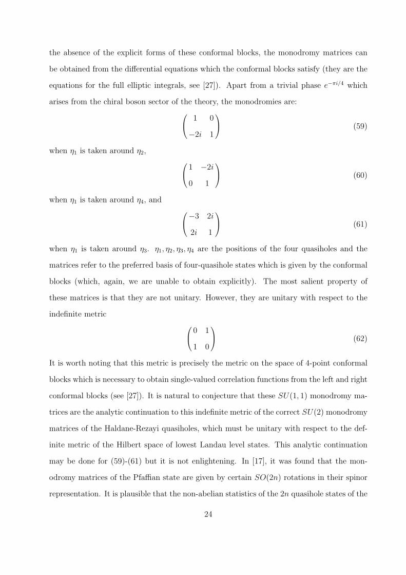
the absence of the explicit forms of these conformal blocks, the monodromy matrices can

be obtained from the differential equations which the conformal blocks satisfy (they are the

equations for the full elliptic integrals, see [27]). Apart from a trivial phase e−πi/4 which

arises from the chiral boson sector of the theory, the monodromies are: 1 0

−2i 1

(59)

when η1 is taken around η2, 1 −2i

0 1

(60)

when η1 is taken around η4, and −3 2i

2i 1

(61)

when η1 is taken around η3. η1, η2, η3, η4 are the positions of the four quasiholes and the

matrices refer to the preferred basis of four-quasihole states which is given by the conformal

blocks (which, again, we are unable to obtain explicitly). The most salient property of

these matrices is that they are not unitary. However, they are unitary with respect to the

indefinite metric 0 1

1 0

(62)

It is worth noting that this metric is precisely the metric on the space of 4-point conformal

blocks which is necessary to obtain single-valued correlation functions from the left and right

conformal blocks (see [27]). It is natural to conjecture that these SU(1, 1) monodromy ma-

trices are the analytic continuation to this indefinite metric of the correct SU(2) monodromy

matrices of the Haldane-Rezayi quasiholes, which must be unitary with respect to the def-

inite metric of the Hilbert space of lowest Landau level states. This analytic continuation

may be done for (59)-(61) but it is not enlightening. In [17], it was found that the mon-

odromy matrices of the Pfaffian state are given by certain SO(2n) rotations in their spinor

representation. It is plausible that the non-abelian statistics of the 2n quasihole states of the

24

Haldane-Rezayi state is given by a reducible representation of some group G (and, hence,

of the braid group) because states of different spins will not mix. One possibility is that the

states can be grouped into a direct sum of the SO(2n) or SU(n) irreducible representations

into which a product of SO(2n) spinor representations may be decomposed.

VI. RELATIONSHIP BETWEEN C = −2 AND C = 1 THEORY.

A number of papers have established a relationship between the the partition functions of

c = −2 and c = 1, R = 1 theories (ie. the c = 1 theory of a Dirac fermion or a free boson with

compactification radius R = 1) [34], [28]. While the proof requires a careful construction of

c = −2 characters taking into account the presence of the logarithmic operators (ref. [34]),

there is a way to roughly understand the relationship in rather simple terms (see, especially,

[40]).

One can easily check that for each operator of dimension hc=−2 in the c = −2 theory

there is an operator of dimension hc=1 in the c = 1, R = 1 theory such that

hc=−2 −−2

24= hc=1 −

1

24(63)

Therefore, in the theory on the cylinder, where the partition function is computed, and

where the edge theory lives, their zero-point energies are the same.

Moreover, for each descendant state in the c = −2 theory there is a corresponding state

in the c = 1, R = 1 theory. Indeed, take the latter theory as represented by a Dirac fermion

S =∫ψ†∂ψ (64)

The modes ψ†n and ψ−n, n > 0 can be used to construct descendant states,

ψ†n1. . . ψ†nα

ψ−m1 . . . ψ−mβ|0〉 (65)

which have the same energies and momenta as the states created by θ−n and θ−n,

θ−n1 . . . θ−nα θ−m1 . . . θ−mβ|0〉 (66)

25

The mode expansion of the field ψ (on the plane) is

ψ(z) =∑n

ψnz−n− 1

2 (67)

so the Dirac fermion has half-integral momenta in the untwisted sector and integral momenta

in the twisted sector, while the opposite is true for the c = −2 theory. Therefore, we map

the twisted sector of c = −2 into the untwisted one of c = 1 and vice versa. (See [40] for a

more detailed discussion of the mapping at the level of the mode expansions.)

Of course, there is still a question of the zero modes ξ; they do not seem to correspond

to anything in c = 1. However, the zero modes ξ are rather special fields. They must be

present as out- (or in-) states of the c = −2 theory to make the correlators of the theory

nonzero, and they have to be present only once (since ξ2 = 0).

As far as many of their conformal properties are concerned, the theories of anticommuting

bosons and of Dirac fermions are the same on the cylinder. Their respective vacua have the

same energy and for each operator of c = −2 theory there exists an operator at c = 1, R = 1.

However, the higher modes of the energy-momentum tensor are different in the two theories.

Consequently, the Virasoro algebra representations are different; in the c = 1 theory, they

are unitary while in the c = −2 theory they are non-unitary.

To understand the equivalence of the c = −2 and c = 1 theories better, let us take a closer

look at the sectors of the c = −2 theory. Ordinarily, each primary field φ(z) of a conformal

field theory and all its descendants generate a highest weight representation of the Virasoro

algebra, perhaps with a chiral symmetry algebra (see rf. [37]). Moreover, that representation

is irreducible. We achieve its irreducibility by removing all the descendants of the primary

field which are themselves primary operators. The Hilbert space of a conformal field theory

can then be written as a direct sum over irreducible highest weight representations.

The problem we immediately encounter in the c = −2 theory is that its states do not

constitute ordinary irreducible highest weight representations of the maximally extended

chiral symmetry algebra (W-algebra) or even of the Virasoro algebra itself. We know that

we have a state there, |I〉, such that L0|I〉 = |0〉, |0〉 being the vaccuum while |I〉 = I(0)|0〉.

26

|I〉 and |0〉 have to be considered together, and together they are usually referred to as a

reducible but indecomposable representation (ref. [29]). Indeed, we can certainly reduce it

by considering a subset of it, consisting of |0〉 and its descendants only, without |I〉. However,

we cannot decompose it into a direct product of |0〉 and |I〉 as L0|I〉 = |0〉.

According to [28], [29], [36] there are four sectors generated by operators with hc=−2 ∈

{−18, 0, 3

8, 1}, denoted V−1/8,R0,V3/8,R1 in the following (we use the notation of [28]) and

the characters of these representations are

χV−1/8=

1

η(τ)Θ0,2(τ) (68)

χV3/8=

1

η(τ)Θ2,2(τ)

χR0 = χR1 =2

η(τ)Θ1,2(τ)

where η(τ) = q1/24∏n>0(1 − qn) is the Dedekind eta function, Θλ,k =

∑n∈Z q

(2kn+λ)2/4k are

ordinary Theta functions, and q = exp(2πiτ) is the modular parameter of the torus.

Note the multiplicity of 2 in the last two characters. It forces an overall multiplicity of

4 in the diagonal partition function to ensure modular invariance7

Zc=−2 = |χR0|2 + |χR1|2 + |2χV−1/8|2 + |2χV3/8

|2 = 4Zc=1(R = 1) (69)

such that equivalence of the partition functions of the c = −2 theory and the c = 1 theory

is really established only up to a factor of 4. Moreover, there is no way to avoid the

multiplicities of the V−1/8 and V3/8 representations. The overall multiplicity of 4 stems from

7Moular invariance of the torus partition function of a conformal field theory is an important

requirement for consistency. In the context of the theory of the bulk of a quantum Hall state, it is

just the statement that the theory, when put on the torus, should be independent of the coordinate

system on the torus. It has been proven [38] that conformal invariance of a theory on S2 implies

modular invariance on the torus, if L0 is diagonal. This should extend to the case of logarithmic

conformal field theory by the limiting procedure described in [34].

27

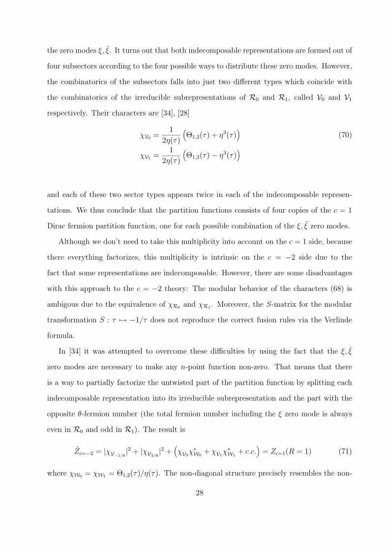
the zero modes ξ, ξ. It turns out that both indecomposable representations are formed out of

four subsectors according to the four possible ways to distribute these zero modes. However,

the combinatorics of the subsectors falls into just two different types which coincide with

the combinatorics of the irreducible subrepresentations of R0 and R1, called V0 and V1

respectively. Their characters are [34], [28]

χV0 =1

2η(τ)

(Θ1,2(τ) + η3(τ)

)(70)

χV1 =1

2η(τ)

(Θ1,2(τ)− η3(τ)

)

and each of these two sector types appears twice in each of the indecomposable represen-

tations. We thus conclude that the partition functions consists of four copies of the c = 1

Dirac fermion partition function, one for each possible combination of the ξ, ξ zero modes.

Although we don’t need to take this multiplicity into account on the c = 1 side, because

there everything factorizes, this multiplicity is intrinsic on the c = −2 side due to the

fact that some representations are indecomposable. However, there are some disadvantages

with this approach to the c = −2 theory: The modular behavior of the characters (68) is

ambigous due to the equivalence of χR0 and χR1 . Moreover, the S-matrix for the modular

transformation S : τ 7→ −1/τ does not reproduce the correct fusion rules via the Verlinde

formula.

In [34] it was attempted to overcome these difficulties by using the fact that the ξ, ξ

zero modes are necessary to make any n-point function non-zero. That means that there

is a way to partially factorize the untwisted part of the partition function by splitting each

indecomposable representation into its irreducible subrepresentation and the part with the

opposite θ-fermion number (the total fermion number including the ξ zero mode is always

even in R0 and odd in R1). The result is

Zc=−2 = |χV−1/8|2 + |χV3/8

|2 +(χV0

χ∗W0+ χV1

χ∗W1+ c.c.

)= Zc=1(R = 1) (71)

where χW0 = χW1 = Θ1,2(τ)/η(τ). The non-diagonal structure precisely resembles the non-

28

diagonal structure of the conformal blocks necessary in the c = −2 theory to ensure crossing

symmetry and single valuedness of the four point function, see [27].

We conclude by mentioning that this partition function is certainly modular invarinat,

but the set of characters {χV−1/8, χV3/8

, χV0 , χW0 , χV1 , χW1} is not. One of the results of [34] is

that by introducing a regularizing term ±iα log(q)η3(τ) into χW0 , χW1 , one recovers modular

covariance for the characters. However, the physical meaning of a log(q) term in character

functions remains unclear. As long as α is taken non-zero, one has a well-defined S-matrix

which can be used to calculate fusion coefficients via the Verlinde formula. As shown in [34],

the latter have physical meaning only in the limit α → 0 and coincide then with explicit

results.

VII. EDGE THEORY OF THE HALDANE-REZAYI STATE

The preceeding considerations inspire us to hope for the following happy ending to our

story: the neutral sector of the low-energy edge theory of the Haldane-Rezayi state is a c = 1

Dirac fermion.

How can we show that this assertion is correct? Since a quantum-mechanical theory is

defined by its Hilbert space of states, inner product, and algebra of observable operators, we

must show that these structures are identical for the c = 1 theory and the edge excitations

annihilated by the Hamiltonian (2). Clearly, the Hilbert spaces, (13) and (65), are the same.8

The spectra (assuming that the energy is proportional to the angular momentum, as before)

and, hence, the partition functions are, as well. Of course, the same may be said for the

c = −2 theory (ignoring subtleties associated with the zero modes, ξ, ξ), as we discussed in

8Almost. The twisted sector of the c = 1 Dirac theory has 2 zero modes, while the edge excitations

of the Haldane-Rezayi state begin at angular momentum 1, ie. k = 2π/L. This zero mode must

be projected out of the theory, which can be done very naturally in the truncation from a c = 2

theory described below.

29

the previous section. The observables – such as the local energy and spin densities – and

the inner product must distinguish the correct edge theory. However, these are difficult to

calculate.

In trying to calculate the inner products of the edge excitations (15), we run into a

familiar roadblock: in the absence of a plasma analogy, there is no painless way of doing

this calculation. This complicates matters when we turn to the algebra of observables,

because we are interested in these operators projected into the low-energy subspace. If this

were simply a matter of projecting into the lowest Landau level, it would be no problem.

However, we must project into the zero-energy subspace of the Hamiltonian (2), since this

is the subspace which contains the low-energy edge excitations. If we simply act on a edge

excitation with an operator such as the lowest Landau level projected density operator, the

resulting state will be in the lowest Landau level, but it will no longer be annihilated by the

Hamiltonian (2). Hence we must project the resulting state into the space of edge excitations

annihilated by (2). This projection cannot be performed without a knowledge of the inner

products of states, so we are stuck again.

Ordinarily, this would not worry us too much because the commutator algebra of the

resulting projected operators would be more or less canonical and easily guessed. However,

in the case of the Haldane-Rezayi state, the SU(2) spin symmetry must be realized in an

unusual way because the edge theory contains two real, i.e. Majorana, fermions, say ψ1(x)

and ψ2(x). Their Lagrangian is invariant under the O(2) rotations ψi′ = Oijψj. There is

no local9 SU(2) transformation law which preserves the reality property of the Majorana

spinors. The simplest way of having an SU(2) doublet of fermions is to have two complex,

i.e. Dirac, spinors, χi, which transform as χi′ = Uijχj. However, since a single Dirac spinor

is composed of two Majorana spinors, such a theory will have too many states at each energy

level. Since the SU(2) symmetry cannot be realized in the standard way, the algebra of the

9i.e. so that ψi′(x) depends only ψj(x) and not on ψj(x′) for x′ 6= x

30

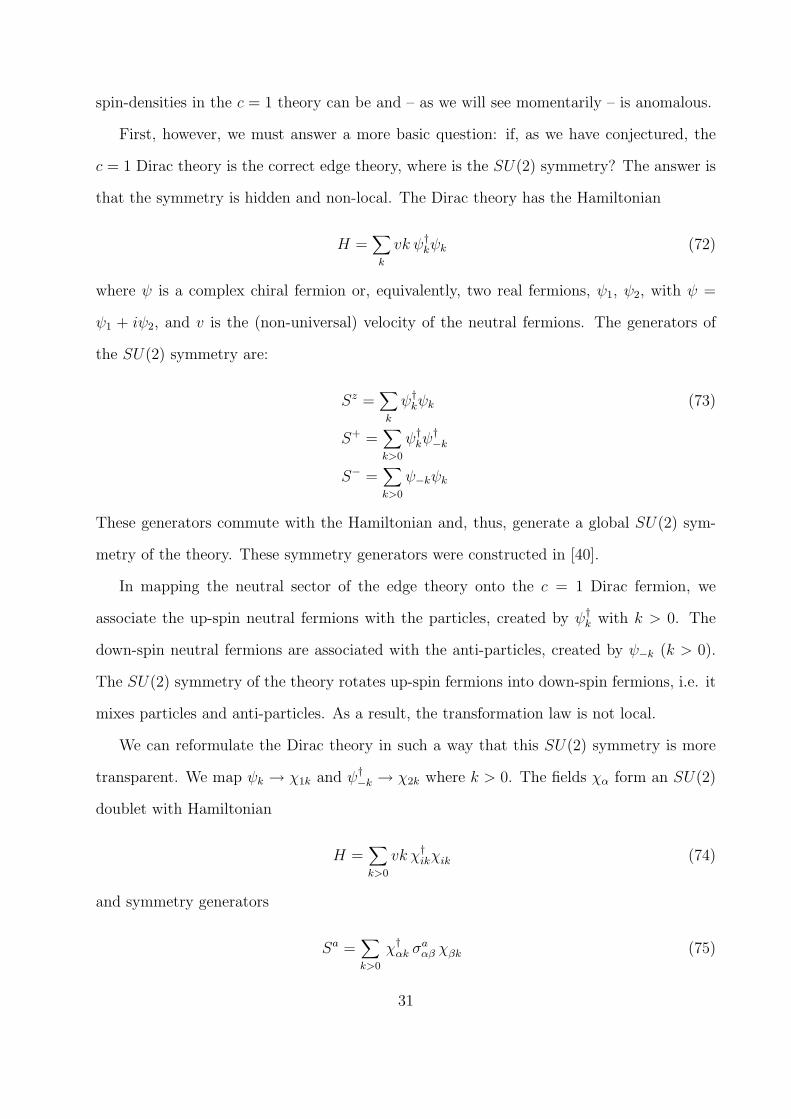
spin-densities in the c = 1 theory can be and – as we will see momentarily – is anomalous.

First, however, we must answer a more basic question: if, as we have conjectured, the

c = 1 Dirac theory is the correct edge theory, where is the SU(2) symmetry? The answer is

that the symmetry is hidden and non-local. The Dirac theory has the Hamiltonian

H =∑k

vk ψ†kψk (72)

where ψ is a complex chiral fermion or, equivalently, two real fermions, ψ1, ψ2, with ψ =

ψ1 + iψ2, and v is the (non-universal) velocity of the neutral fermions. The generators of

the SU(2) symmetry are:

Sz =∑k

ψ†kψk (73)

S+ =∑k>0

ψ†kψ†−k

S− =∑k>0

ψ−kψk

These generators commute with the Hamiltonian and, thus, generate a global SU(2) sym-

metry of the theory. These symmetry generators were constructed in [40].

In mapping the neutral sector of the edge theory onto the c = 1 Dirac fermion, we

associate the up-spin neutral fermions with the particles, created by ψ†k with k > 0. The

down-spin neutral fermions are associated with the anti-particles, created by ψ−k (k > 0).

The SU(2) symmetry of the theory rotates up-spin fermions into down-spin fermions, i.e. it

mixes particles and anti-particles. As a result, the transformation law is not local.

We can reformulate the Dirac theory in such a way that this SU(2) symmetry is more

transparent. We map ψk → χ1k and ψ†−k → χ2k where k > 0. The fields χα form an SU(2)

doublet with Hamiltonian

H =∑k>0

vk χ†ikχik (74)

and symmetry generators

Sa =∑k>0

χ†αk σaαβ χβk (75)

31

As a result of the restriction to k > 0, they are ‘half’ of an SU(2) doublet of Dirac fermions.

The k < 0 part of the theory has been discarded. It then follows that there is no local SU(2)

Kac-Moody algebra. If we introduce local spin densities, Sa(x) and their Fourier transforms,

Saq =

∑k>0

χ†αk+q σaαβ χβk (76)

we find that their commutators do not close because the sums over k are restricted to k > 0.

In particular, their commutators are not local, i.e. [Sa(x), Sb(x′)] ∝ 1/(x − x′) rather than

[Sa(x), Sb(x′)] ∝ δ(x− x′).

This might appear to be a death blow to the c = 1 theory of the neutral sector. In the

underlying quantum mechanics of electrons, these commutators are local, i.e. proportional

to δ-functions, so we would expect that in the low-energy theory they would be, at worst,

δ-functions smeared out at the scale of the cutoff. However, this argument is a bit too quick.

The cutoff in this theory is O(V1) (see (2)) meaning that our edge theory is an effective field

theory for energies less than O(V1). However, unlike in a Euclidean or relativistic theory,

this energy scale does not imply a length scale. While the theory must be local in time

(again, modulo non-localities at scales smaller than the cutoff), it does not necessarily have

commutators which are local in space.

But do the spin-densities, projected into the low-energy subspace actually have such a

non-local algebra? If not, the c = 1 theory must be ruled out. If so – and, as we argued

above this would not contradict any fundamental principle which is dear to our hearts –

then the c = 1 theory is a viable candidate to describe the neutral sector of the edge of the

Haldane-Rezayi state. Consider the following state, where PH is the projection operator

into the zero-energy subspace of (2):

PH S+(w)PH · Ψ0 = (77)

PH A(e(2wz1−|w|2−|z1|2)/4`20

u1u2

(w − z2)2

u3v4 − v3u4

(z3 − z4)2. . .

)∏i>1

(w − zi)2∏

k>l>1

(zk − zl)2 e

− 1

4`20

∑i>1

|zi|2

which results from acting on the ground state with the local projected S+(w) operator. It is

quite plausible that the right-hand-side vanishes upon projection. This would agree with the

32

c = 1 theory, where S+(x)|0〉 =∑

k>0,q eiqx χ†αk σ

+αβ χβk|0〉 = 0 because χβk|0〉 = 0 for k > 0.

For a doublet of Dirac fermions (and presumably for any other theory with a local SU(2)

transformation law), on the other hand, the k < 0 modes will give a non-zero contribution.

Furthermore, suppose we act with this operator on a state with 1 neutral fermion:

PH S+(w)PH · A

(zk1v1

u2v3 − v2u3

(z2 − z3)2. . .

)∏(zi − zj)

2 = (78)

PHA(e(2wz1−|w|2−|z1|2)/4`20 wku1

u2v3 − v2u3

(z2 − z3)2. . .

)∏i>1

(w − zi)2∏

k>l>1

(zk − zl)2 e

− 1

4`20

∑i>1

|zi|2

+ terms in which the spin acts on paired electrons

If this is non-vanishing, it is plausibly equal to (the aj are some, possibly w-dependent,

coefficients):

A

∑j

ajzj1 w

ku1u2v3 − v2u3

(z2 − z3)2. . .

∏i>j

(zi − zj)2 e

− 1

4`20

∑i|zi|2

(79)

If so, then the up-spin electron (and its concomitant neutral fermion) is no longer localized

at w because of the large powers of z1 from the Jastrow factor. In such a case, however,

when we act with another local spin operator, S−(w′), the commutator, which receives non-

vanishing contributions only when the two spin operators act on the same electron, need

not vanish for w 6= w′ (or, rather, need not decay as a Gaussian in w − w′).

Even if our hypothesis is incorrect, and the Haldane-Rezayi edge theory is some other

theory, it is difficult to see how the SU(2) symmetry could be local. There are simply ‘too

few’ single fermion states, by a factor of two, to allow for a local SU(2) symmetry. This is

quite clear from the formulation as a truncated Dirac doublet. If we were to take an inner

product different from the inner product of the c = 1 theory, this would not help matters

since it could not increase the size of the Hilbert space. Could it be that we have simply

chosen the wrong symmetry generators? This is unlikely since the symmetry generators

(75) have the desired action: they rotate the spins of the fermions. In principle, there is

one other possibility. If there were low-energy excitations in the bulk withh anomalous total

derivative terms in their SU(2) algebra, these terms could cancel the anomalous terms at

the edge. However, there is no trace of such excitations among the states annihilated by (2).

33

VIII. EXPERIMENTAL CONSEQUENCES.

If our hypothesis is correct and the edge theory of the Haldane-Rezayi state is the c = 1+1

conformal field theory, there are measurable consequences which could elucidate the nature

of the ν = 52

plateau. The electron annihilation operator is ψe−i√

2φ, so the coupling to a

Fermi liquid lead will be ψe−i√

2φ Ψlead. This is a dimension 2 operator, so the tunneling

conductance, Gt, through a point contact between a Fermi liquid lead and the edge of the

Haldane-Rezayi state is

Gt ∼ T 2 (80)

See [10,11] to compare (80) with the corresponding expression for a Laughlin state. If the

voltage V � T , then I ∼ V 3. For tunneling between two Haldane-Rezayi droplets, Gt ∼ T 4

for T � V and I ∼ V 5 for T � V . The tunneling of quasiparticles from one edge of

a Haldane-Rezayi droplet to another through the bulk is presumably dominated by the

tunneling of half-flux quantum quasiparticles, which are created by µe−iφ/2√

2 where µ is

the Dirac theory twist field. The resulting tunneling conductance between the two edges is

Gt ∼ T−5/4 at high temperatures; at low temperature it is 12

e2

hwith corrections determined

by the perturbations of a strong-coupling fixed point.

One thing which is, perhaps, surprising about these predictions is that they are precisely

the same as would be expected for the (3, 3, 1) state and for a simple reason: the edge

theories are almost the same. According to [19], the neutral sector of the (3, 3, 1) state is a

c = 1 Dirac fermion. The only difference with the edge theory of the Haldane-Rezayi state is

that the twisted and untwisted sectors are exchanged, but this does not affect the dimensions

of the scaling operators which determine the above power laws. Hence, the Haldane-Rezayi

and (3, 3, 1) states cannot be distinguished from simple tunneling experiments at the edge.

However, these states are definitely not in the same universality class. Their bulk excitations

have different topological properties, as may be seen from the ground state degeneracy on

the torus. In an Aharonov-Bohm experiment with two half-flux quantum quasiholes, the

34

phase resulting when one winds around another is 3πi/4 in the Haldane-Rezayi state (from

(56)) but −πi/8 in the (3, 3, 1) state (and 0 in the Pfaffian state). In experiments with

more than two quasiholes, the full structure of the non-Abelian statistics of the Haldane-

Rezayi state comes into play and, again, Aharonov-Bohm experiments can resolve it from

the (3, 3, 1) and other candidate quantum Hall states.

ACKNOWLEDGMENTS

This work would not have been possible without the help, advice, and encouragement,

given to us by a number of people, particularly L. Balents, M.P.A. Fisher, K. Gawedzki,

F.D.M. Haldane, B.I. Halperin, A.W.W. Ludwig, M. Moriconi, J. Polchinski, V. Sadov, T.

Spencer, A.M. Tikofsky, P.B. Wiegmann, F. Wilczek, and A.B. Zamolodchikov.

35

REFERENCES

[1] R.L. Willet, et al., Phys. Rev. Lett. 59 (1987) 1776

[2] F.D.M. Haldane and E.H. Rezayi, Phys. Rev. Lett. 60 (1988) 956; 1886.

[3] X.G. Wen, Int. J. Mod. Phys. B2 (1990) 239; Phys. Rev. B40 (1989) 7387. X.G. Wen

and Q. Niu, Phys. Rev. B41 (1990) 9377.

[4] S.M. Girvin and A.H. MacDonald, Phys. Rev. Lett. 58 (1987) 1252. S.C. Zhang, T.H.

Hansson, and S. Kivelson, Phys. Rev. Lett. 62 (1988) 82. N. Read, Phys. Rev. Lett. 62

(1988) 86.

[5] B.I. Halperin, Phys. Rev. Lett. 52 (1984) 1583; 52 2390(E).

[6] D.P. Arovas, J.R. Schrieffer, and F. Wilczek, Phys. Rev. Lett. 53 (1984) 722.

[7] A. Cappelli, et al., Nucl. Phys. B448 (1995) 470; DFF-249-5-96, hep-th/9605127.

[8] G. Christofano, et al., Nucl. Phys. Proc. Suppl. 33C (1993) 119; Phys. Lett. B262

(1991) 88.

[9] J. Frohlich and A. Zee, Nucl. Phys. B364 (1991) 517.

[10] X.G. Wen, Phys. Rev. B43 (1991) 11025; Int. J. Mod. Phys. B6 (1992) 1711, and

references therein.

[11] C.L. Kane and M.P.A. Fisher, Phys. Rev. B46 (1992) 15223.

[12] P. Fendley, A.W.W. Ludwig, and H. Saleur, Phys. Rev. Lett. 74 (1995) 3005.

[13] F.P. Millikan, C.P. Umbach, and R. Webb, Solid State Comm. 97 (1996) 309.

[14] A.M. Chang, et al., Phys. Rev. Lett. 77 (1996) 2538.

[15] G. Moore and N. Read, Nucl. Phys. B360 (1991) 362.

[16] E. Witten, Comm. Math. Phys. 121 (1989) 351.

36

[17] C. Nayak and F. Wilczek, Nucl. Phys. B479 (1996) 529.

[18] X.G. Wen, Y.S. Wu, Nucl. Phys. B419 (1994) 455.

[19] M. Milovanovic and N. Read, Phys. Rev. B53 (1996) 13559.

[20] F.D.M. Haldane, Bull. of A.P.S. 35 (1990) 254. M. Stone, Ann. Phys. 207 (1991) 38;

Int. Jour. Mod. Phys. B5 (1991) 509.

[21] B.I. Halperin, Helv. Phys. Act. 56 (1983) 75.

[22] M. Greiter, X.G. Wen, and F. Wilczek, Nucl. Phys. B374 (1992) 567.

[23] T.L. Ho, Phys. Rev. Lett. 75 (1995) 1186.

[24] N. Read and E.H. Rezayi, cond-mat/9609079.

[25] E. Keski-Vakkuri and X.G. Wen, Intl. J. Mod. Phys. B7 (1993) 4227.

[26] B. Blok and X.G. Wen, Nucl. Phys. B374 (1992) 615.

[27] V. Gurarie, Nucl. Phys. B410 (1993) 535; hep-th/9303160

[28] M.R. Gaberdiel, H.G. Kausch, Phys. Lett. B386 (1996) 131; hep-th/9606050

[29] M.R. Gaberdiel, H.G. Kausch, Nucl. Phys. B477 (1996) 293

[30] H.G. Kausch, DAMTP-95-52, Oct. 1995; hep-th/9510149

[31] J.S. Caux, I.I. Kogan, A.M. Tsvelik, Nucl. Phys. B466 (1996) 444; hep-th/9511134.

[32] D. Friedan, E. Martinec, S. Shenker, Nucl. Phys. B271 (1986) 93

[33] H.G. Kausch, Phys. Lett. B259 (1991) 448

[34] M.A.I. Flohr, Int. J. Mod. Phys. A11 (1996) 4147; M.A.I. Flohr, hep-th/9605151, to

be published in Int. J. Mod. Phys.

[35] L.S. Georgiev and I.T. Todorov, INRNE-TH-96-13, hep-th/9611084.

37

[36] F. Rohsiepe, BONN-TH-96-17, Nov. 1996; hep-th/9611160

[37] A.A. Belavin, A.M. Polyakov, and A.B. Zamolodchikov, Nucl. Phys. B241 (1984) 333.

[38] W. Nahm Int. J. Mod. Phys. A6 (1991) 2837; in Proc. Trieste July 1990 Topological

methods in quantum field theories, World Scientific, 1991.

[39] The authors are grateful to A.B. Zamolodchikov for pointing out that I, as well as any

other local field, can be expressed in terms of the fundamental fields θ and θ of the

theory.

[40] While we were completing this paper, a preprint, hep-th/9612172, by S. Guruswamy

and A.W.W. Ludwig appeared in which the relationship between the c = 1 and c = −2

theories was discussed and the hidden symmetry of the c = 1 theory was constructed.

38