The Group Lasso for Logistic Regression

Lukas Meier Sara van de Geer Peter Buhlmann

February 8, 2007

Abstract

The Group Lasso (Yuan and Lin, 2006) is an extension of the Lasso to do vari-able selection on (predefined) groups of variables in linear regression models. Theestimates have the attractive property of being invariant under groupwise orthog-onal reparametrizations. We extend the Group Lasso to logistic regression modelsand present an efficient algorithm, especially suitable for high-dimensional problems,which can also be applied to more general models to solve the corresponding convexoptimization problem. The Group Lasso estimator for logistic regression is shown tobe statistically consistent even if the number of predictors is much larger than samplesize but with sparse true underlying structure. We further use a two-stage procedurewhich produces sparser models than the Group Lasso, leading to improved predictionperformance for some cases. Moreover, due to the two-stage nature, the estimatescan be constructed to be hierarchical. The methods are used on simulated and realdatasets about splice site detection in DNA sequences.

1 Introduction

The Lasso (Tibshirani, 1996), originally proposed for linear regression models, has becomea popular model selection and shrinkage estimation method. In the usual linear regressionsetup we have a continuous response Y ∈ R

n, an n× p design matrix X and a parametervector β ∈ R

p. The Lasso estimator is then defined as

βλ = arg minβ

‖Y −Xβ‖22 + λ

p∑

i=1

|βi| ,

where ‖u‖22 =∑n

i=1 u2i for a vector u ∈ R

n. For large values of the penalty parameter

λ, some components of βλ are set exactly to zero. The `1-type penalty of the Lassocan also be applied to other models as for example Cox regression (Tibshirani, 1997),logistic regression (Lokhorst, 1999; Genkin et al., 2004) or multinomial logistic regression(Krishnapuram et al., 2005) by replacing the residual sum of squares by the correspondingnegative log-likelihood function.

Already for the special case in linear regression when not only continuous but also cat-egorical predictors (factors) are present, the Lasso solution is not satisfactory as it onlyselects individual dummy variables instead of whole factors. Moreover, the Lasso solutiondepends on how the dummy variables are encoded. Choosing different contrasts for acategorical predictor will produce different solutions in general. The Group Lasso (Yuan

1

and Lin, 2006; Bakin, 1999) overcomes these problems by introducing a suitable extensionof the Lasso penalty. The estimator is defined as

βλ = arg minβ

‖Y −Xβ‖22 + λG∑

g=1

‖βIg‖2,

where Ig is the index set belonging to the gth group of variables, g = 1, . . . , G. Thispenalty can be viewed as an intermediate between the `1- and `2-type penalty. It has theattractive property that it does variable selection at the group level and is invariant under(groupwise) orthogonal transformations like Ridge regression (Yuan and Lin, 2006).

This article deals with the Group Lasso penalty for logistic regression models. The logisticcase calls for new computational algorithms. We present efficient methods whose conver-gence property does not depend on unknown constants as in Kim et al. (2006). We donot aim for an (approximate) path-following algorithm (Rosset, 2005; Zhao and Yu, 2004;Park and Hastie, 2006a,b) but our approaches are fast enough for computing a whole rangeof solutions for varying penalty parameters on a (fixed) grid. Our approach is related toGenkin et al. (2004) which presents an impressively fast implementation (“the fastest”)for large-scale logistic regression with the Lasso. Moreover, we present an asymptoticconsistency theory for the Group Lasso in high-dimensional problems where the predictordimension is much larger than sample size. This has neither been developed for linear norlogistic regression. High-dimensionality of the predictor space arises in many applications,in particular with higher-order interaction terms or basis expansions for logistic additivemodels where the groups correspond to the basis functions for individual continuous co-variates. Our application about the detection of splice sites, the regions between coding(exons) and non-coding (introns) DNA segments involves the categorical predictor space{A,C,G, T}7 which has cardinality 16’384.

The rest of this arcticle is organized as follows: In Section 2 we restate in more detail theidea of the Group Lasso for logistic regression models, develop two efficient algorithmswhich are proven to solve the corresponding convex optimization problem and comparethem with other optimization methods. Furthermore, we show that the Group Lassoestimator is statistically consistent for high-dimensional, sparse problems. In Section 3we outline a two-stage procedure which often produces more adequate models both interms of model size and prediction performance. Simulations follow in Section 4 and anapplication of the modeling of functional DNA sites can be found in Section 5. Section 6contains the discussion. All proofs are given in the Appendix.

2 Logistic Group Lasso

2.1 Model Setup

Assume we have i.i.d. observations (xi, yi), i = 1, . . . , n of a p-dimensional vector xi ∈ Rp of

G predictors and a binary response variable yi ∈ {0, 1}. Both categorical and continuouspredictors are allowed. We denote by dfg the degrees of freedom of the gth predictorand can thus rewrite xi = (xT

i,1, . . . ,xTi,G)T with the group of variables xi,g ∈ R

dfg , g =1, . . . , G. For example, the main effect of a factor with 4 levels has df = 3 while acontinuous predictor involves df = 1 only.

2

Linear logistic regression models the conditional probability pβ(xi) = Pβ[Y = 1 |xi] by

log

(pβ(xi)

1− pβ(xi)

)= ηβ(xi), (2.1)

with

ηβ(xi) = β0 +G∑

i=1

xTi,gβg,

where β0 is the intercept and βg ∈ Rdfg is the parameter vector corresponding to the gth

predictor. We denote by β ∈ Rp+1 the whole parameter vector, i.e. β = (β0,β

T1 , . . . ,βT

G)T .

The Logistic Group Lasso estimator βλ is given by the minimizer of the convex function

Sλ(β) = −`(β) + λ

G∑

g=1

s(dfg)‖βg‖2, (2.2)

where `(·) is the log-likelihood function, i.e.

`(β) =

n∑

i=1

yiηβ(xi)− log (1 + exp{ηβ(xi)}).

The tuning parameter λ ≥ 0 controls the amount of penalization. Note that we do notpenalize the intercept. However, as shown in Lemma 2.1, the minimum in (2.2) is attained.The function s(·) is used to rescale the penalty with respect to the dimensionality of theparameter vector βg. Unless stated otherwise, we use s(dfg) =

√dfg to ensure that the

penalty term is of the order of the number of parameters dfg. The same rescaling is usedin Yuan and Lin (2006).

Lemma 2.1. For λ > 0 and s(d) > 0 for all d ∈ N, the minimum in optimization problem(2.2) is attained.

The “groupwise” `2-norm in (2.2) is an intermediate between the Lasso and the Ridgepenalty function. It encourages that in general either βg = 0 or βg,j 6= 0 for all j ∈{1, . . . , dfg}, where we have omitted the index λ for easier notation. A geometrical inter-pretation of this special sparsity property is given in Yuan and Lin (2006). An exampleof a solution path {βλ}λ≥0 for a model consisting of an intercept and two factors having3 degrees of freedom each is depicted in figure 1.

Let the n× dfg matrix Xg be the columns of the design matrix corresponding to the gthpredictor. If we assume that the block matrices Xg are of full rank, we can perform a(blockwise) orthornomalization – e.g. by a QR-decomposition – to get X T

g Xg = Idfg, g =

1, . . . , G. Using such a design matrix, the Group Lasso estimator does not depend on theencoding scheme of the dummy variables. We choose a rescaled version X T

g Xg = n · Idfg

to ensure that the parameter estimates are on the same scale when varying the samplesize n. After parameter estimation, the estimates have to be transformed back in order tocorrespond to the original encoding.

2.2 Algorithms for the Logistic Group Lasso

2.2.1 Block Coordinate Descent

Parameter estimation is computationally more demanding than for linear regression mod-els. The algorithm presented in Yuan and Lin (2006) sequentially solves a system of

3

0.0 0.1 0.2 0.3 0.4 0.5 0.6 0.7 0.8 0.9 1.0

−0.6

−0.2

0.2

0.6

λ λmax

Par

amet

er e

stim

ates

Figure 1: Solution path {βλ}λ≥0 for a model consisting of an intercept (dotted line) andtwo factors having 3 degrees of freedom each (dashed and solid lines, respectively).

(necessary and sufficient) non-linear equations which corresponds to a groupwise mini-mization of the penalized residual sum of squares, but no result on numerical convergenceis given. For the more difficult case of logistic regression, we can also use a block co-ordinate descent algorithm and we prove numerical convergence by using the results ofTseng (2001) as shown in Proposition 2.1. The key lies in the separable structure of thenon-differentiable part in Sλ.

We cycle through the parameter groups and minimize the objective function Sλ, keepingall but the current parameter group fixed. This leads us to the algorithm presented intable 1, where we denote by β−g the parameter vector β when setting βg to 0 while allother components remain unchanged. In step (3) we first check whether the minimum isat the non-differentiable point βg = 0. If not, we can use a standard numerical minimizer,e.g. a Newton type algorithm, to find the optimal solution with respect to βg. In sucha case the values of the last iteration can be used as starting values to save computingtime. If the group was not in the model in the last iteration, we first go a small step in theopposite direction of the gradient of the negative log-likelihood function to ensure that westart at a differentiable point.

Proposition 2.1. Step (2) and (3) of the block coordinate descent algorithm performgroupwise minimizations of Sλ and are well defined in the sense that the correspondingminima are attained. Furthermore, if we denote by β(t) the parameter vector after t blockupdates, then every limit point of the sequence {β(t)}t≥0 is a minimum point of Sλ.

Because the iterates can be shown to stay in a compact set, the existence of a limit pointis guaranteed.

The main drawback of such an algorithm is that the blockwise minimizations of the active

4

Logistic Group Lasso Algorithm (Block Coordinate Descent)

(1) Let β ∈ Rp+1 be an inital parameter vector.

(2) β0 ← arg minβ0

Sλ(β)

(3) for g = 1, . . . , Gif ‖XT

g (y − pβ−g)‖2 ≤ λs(dfg)

βg ← 0

elseβg ← arg min

βg

Sλ(β)

endend

(4) Repeat step (2)–(3) until some convergence criteria is met.

Table 1: Logistic Group Lasso Algorithm using Block Coordinate Descent Minimization.

groups have to be performed numerically. However, for small and moderate sized problemsin the dimension p and the group sizes dfg this turns out to be sufficiently fast. For large-scale applications it would be attractive to have a closed form solution for a block updateas in Yuan and Lin (2006). This will be discussed in the next subsection.

2.2.2 Block Coordinate Gradient Descent

The key idea of the block coordinate gradient descent method of Tseng and Yun (2006)is to combine a quadratic approximation of the log-likelihood with an additional linesearch. Using a second order Taylor expansion at β(t) and replacing the Hessian of thelog-likelihood function `(·) by a suitable matrix H (t) we define

M(t)λ (d) = −

{`(β(t)) + dT∇`(β(t)) +

1

2dT H(t)d

}+ λ

G∑

g=1

s(dfg)‖β(t)g + dg‖2 (2.3)

≈ Sλ(β(t) + d),

where d ∈ Rp+1. Now we consider the minimization of M

(t)λ (·) with respect to the gth

penalized parameter group. This means that we restrict ourselves to vectors d with dk = 0

for k 6= g. Moreover, we assume that the corresponding dfg×dfg submatrix H(t)gg is diagonal,

i.e. H(t)gg = h

(t)g · Idfg

for some scalar h(t)g ∈ R.

If ‖∇`(β(t))g − h(t)g β

(t)g ‖2 ≤ λs(dfg), the minimizer of (2.3) is

d(t)g = −β(t)

g .

Otherwise

d(t)g = −

1

h(t)g

(∇`(β(t))g − λs(dfg)

∇`(β(t))g − h(t)g β

(t)g

‖∇`(β(t))g − h(t)g β

(t)g ‖2

).

If d(t) 6= 0, an inexact line search using the Armijo rule has to be performed: Let α(t) bethe largest value in {α0δ

l}l≥0 such that

Sλ(β(t) + α(t)d(t))− Sλ(β(t)) ≤ α(t)σ∆(t),

5

Logistic Group Lasso Algorithm (Block Coordinate Gradient Descent)

(1) Let β ∈ Rp+1 be an inital parameter vector.

(2) for g = 0, . . . , GHgg ← hg(β) · Idfg

d← arg mind |dk=0, k 6=g

Mλ(d)

if d 6= 0α← Line searchβ ← β + α · d

endend

(3) Repeat step (2) until some convergence criteria is met.

Table 2: Logistic Group Lasso Algorithm using Block Coordinate Gradient Descent Min-imization.

where 0 < δ < 1, 0 < σ < 1, α0 > 0, and ∆(t) is the improvement in the objective functionSλ when using a linear approximation for the log-likelihood, i.e.

∆(t) = −(d(t))T∇`(β(t)) + λs(dfg)‖β(t)g + d(t)

g ‖2 − λs(dfg)‖β(t)g ‖2.

Finally, we defineβ(t+1) = β(t) + α(t)d(t).

The algorithm is outlined in table 2. When minimizing M(t)λ with respect to a penalized

group, we first have to check whether the minimum is at a non-differentiable point asoutlined above. For the (unpenalized) intercept this is not necessary and the solution canbe directly computed

d(t)0 = −

1

h(t)0

∇`(β(t))0.

For a general matrix H (t) the minimization with respect to the gth parameter group

depends on H(t) only through the corresponding submatrix H(t)gg . To ensure a reasonable

quadratic approximation in (2.3), H(t)gg is ideally chosen to be close to the corresponding

submatrix of the Hessian of the log-likelihood function. Restricting ourselves to diagonal

matrices H(t)gg = h

(t)g · Idfg

, a possible choice is (Tseng and Yun, 2006)

h(t)g = −max

{diag

(−∇2`(β(t))gg

), c∗

}, (2.4)

where c∗ > 0 is a lower bound to ensure convergence (see Proposition 2.2). The matrixH(t) does not necessarily have to be recomputed in each iteration. Under some mildconditions on H (t) convergence of the algorithm is assured as can be seen from Tseng andYun (2006) and from the proof of Proposition 2.2.

Standard choices for the tuning parameters are for example α0 = 1, δ = 0.5, σ = 0.1(Bertsekas, 2003; Tseng and Yun, 2006). Other definitions of ∆(t) as for example toinclude the quadratic part of the improvement are also possible. We refer the reader toTseng and Yun (2006) for more details and proofs that ∆(t) < 0 for d(t) 6= 0 and that theline search can always be performed.

6

Proposition 2.2. If H(t)gg is chosen according to (2.4), then every limit point of the se-

quence {β(t)}t≥0 is a minimum point of Sλ.

It is also possible to update the coordinate blocks in a non-cyclic manner or all at thesame time which would allow for a parallelizable approach with the convergency resultstill holding.

The block coordinate gradient descent algorithm can also be applied to the Group Lassoin other models. For example, any generalized linear model where the response y has adistribution from the exponential family falls into this class.

A related algorithm is found in Krishnapuram et al. (2005), where a global upper boundon the Hessian is used to solve the Lasso problem for multinomial logistic regression. Thisapproach can also be used with the Group Lasso penalty resulting in a closed form solutionfor a block update. However, the upper bound is not tight enough for moderate and smallvalues of λ which leads to too slow convergence in general. Genkin et al. (2004) overcomesthis problem by working with an updated local bound on the second derivative and byrestricting the change of the current parameter to a local neighbourhood.

For linear models, the LARS-algorithm (Efron et al., 2004; Osborne et al., 2000) is veryefficient for computing the path of Lasso solutions {βλ}λ≥0. For logistic regression, ap-proximate path following algorithms have been proposed (Rosset, 2005; Zhao and Yu,2004; Park and Hastie, 2006a). But with the Group Lasso penalty, some of them are notapplicable (Rosset, 2005) or do not necessarily converge to a minimum point of Sλ (Zhaoand Yu, 2004), and all of them do not seem to be computationally faster than workingiteratively on a fixed grid of penalty parameters λ. The latter has been observed as wellby Genkin et al. (2004) for logistic regression with the Lasso in large-scale applications.

To calculate the solutions βλ on a grid of the penalty parameter 0 ≤ λK < . . . < λ1 ≤ λmax

we can for example start at

λmax = maxg∈{1,...,G}

1

s(dfg)‖XT

g (y − y)‖2,

where only the intercept is in the model. We then use βλkas a starting value for βλk+1

and proceed iteratively until βλKwith λK equal or close to zero. Instead of updating the

approximation of the Hessian H (t) in each iteration, we can use a constant matrix basedon the previous parameter estimates βλk

to save computing time, i.e.

H(t)gg = hg(βλk

)Idfg,

for the estimation of βλk+1. Some cross-validation can then be used for choosing the

parameter λ. Most often, we aim for minimal test-sample negative log-likelihood score.

2.3 Comparison with Other Algorithms

In this subsection we compare the Block Coordinate Gradient Descent algorithm (BCGD)with the algorithm of Kim et al. (2006) (BSR, standing for Blockwise Sparse Regression).After an earlier version of this manuscript, Park and Hastie (2006b) (PH) also applied theirmethodology of Park and Hastie (2006a) to Group Lasso models which we also include inour comparison.

7

We emphasize that BSR is a method which requires the specification of an algorithmic tun-ing parameter, denoted by s. It is shown in Kim et al. (2006) that numerical convergenceof BSR only holds if s is chosen sufficiently small (depending on the unknown Lipschitzconstant of the gradient). Moreover, a small parameter s slows down the computationalspeed of BSR, and vice-versa for a large s. Thus, we are in a situation of trading-offnumerical convergence versus computational speed. Our BCGD method does not requirethe specification of an algorithmic tuning parameter to ensure convergence, and we viewthis as a very substantial advantage for practical use.

For comparing the different algorithms, we use a random design matrix where the predic-tors are simulated according to a centered multivariate normal distribution with covariancematrix Σi,j = ρ|i−j|. If not stated otherwise, ρ = 0.5 is used. For the penalty parameterλ multiplicative grids between λmax and λmax/100 are used.

For BCGD we use the R package grplasso and for BSR our own implementation inR. As BSR works with a constraint instead of a penalty, we use the result of BCGDas constraint value. We use an equivalent stopping criteria as in package grplasso, i.e.the relative function improvement and the relative change of the parameter vector haveto be small enough. Although this slowed down the algorithms, it is necessary in orderto identify the correct active set of the solution. For both algorithms we make use ofthe preceding solution of the path as starting value for the next grid point. For BCGDwe update the Hessian at each 5th grid point. For the path-following algorithm PHwe use the corresponding Matlab implementation available at http://www.stanford.

edu/~mypark/glasso.htm. As recommended, the step length on the λ-scale is chosenadaptively. However, we were able to run PH with reasonable computing time on verysmall datasets only.

One of them is motivated by the user guide of PH. It consists of n = 200 observations ofG = 3 groups each having df = 3, i.e. p = 10 (with intercept). For the design matrix we useρ = 0 and the whole parameter vector is set to zero, i.e. there is no signal. 20 grid pointsare used for λ. The corresponding cpu times (in seconds) based on 20 simulation runs are0.093 (0.01), 0.041 (0.0054), 5.96 (1.23) for BCGD, BSR and PH respectively. Standarddeviations are given in parantheses. We used the tuning parameter s = 0.01 for BSR.Already for such a simple, low-dimensional problem, BCGD and BSR were substantiallyfaster than PH. As mentioned above, we could not run PH for larger problems (this isprobably due to implementation, but we also think that an optimized implementation ofPH, involving potentially large active sets, would be slower than BCGD or BSR).

As a second example, we use a higher-dimensional setting with n = 100 and G = 250groups each having df = 4 (p = 1001). The first 10 groups are active with coefficient0.2, resulting in a Bayes risk of approximately 0.2. The computing times based on 20simulation runs are depicted in figure 2, where we have used 100 grid points for λ. Theboxplot for s0 = 0.025 is dashed because the probability for numerical convergence wasonly 20%. BSR with s suitably chosen is not faster in this example. The success fornumerical convergence depends heavily on the choice of s and additional time is neededto find an optimal value for s. For some single λ values, BSR sometimes turned out to befaster, but the difference between the computing times when calculating the whole pathis much smaller due to good starting values and the fact that BSR slows down for smallvalues of λ.

We also applied BSR to the splice site dataset in Section 5. The running times are reportedin table 3. We summarize that BCGD is often almost as fast or even faster (as for the

8

020

4060

8010

012

0

CP

U ti

me

[s]

BCGD s0 = 0.025 s0 ⋅ 1 2 s0 ⋅ 1 4 s0 ⋅ 1 8 s0 ⋅ 1 16

Figure 2: CPU times for BCGD (left) and for BSR with different values of the parameters. See text for more details.

BCGD s = 5 · 10−4 s = 2.5 · 10−4 s = 1.25 · 10−4 s = 6.125 · 10−5

948 2737 4273 6688 10581

Table 3: CPU times on the splice site dataset for BCGD (left) and for BSR with differentvalues for the parameter s. The algorithm did not converge for larger values of s.

real splice site dataset) as BSR with the optimal algorithmic tuning parameter s. Thistuning parameter varies very much from problem to problem, and it is highly unrealisticto have reasonable a-priori knowledge about a good parameter. Thus, the user needs todo some trial-and-error first which can be very unpleasant. In contrast, BCGD runs fullyautomatic and is proved to converge, as described in Section 2.2.2.

The fact that coordinate-wise approaches for sparse models are efficient for high-dimensionaldata has also been noticed by Genkin et al. (2004) or Balakrishnan and Madigan (2006).They have successfully applied related algorithms for the Lasso even when the number ofvariables was in the hundreds of thousands. For the coordinate-wise approaches in gen-eral, already after a few sweeps through all variables, both the objective function and thenumber of selected variables is close to the optimal solution.

2.4 Consistency

A reasonable choice of the tuning parameter λ will depend on the sample size n, as wellas on the number of groups G, and the degrees of freedom within each group. Assumingthe degrees of freedom per group is kept fixed, the smoothing parameter λ can be takenof order log G. Then the Group Lasso can be shown to be globally consistent undersome further regularity and sparseness conditions. This section gives more details on thisasymptotic result.

9

Let us consider the data (before rescaling) (xi, yi) as independent copies of the populationvariable (x, y). The negative log-likelihood function is used as loss function which wedenote for easier notation by

γβ(x, y) = − [yηβ(x)− log(1 + exp{ηβ(x)})] .

The theoretical risk is defined as

R(β) = E [γβ(x, y)] ,

and the empirical counterpart as

Rn(β) =1

n

n∑

i=1

γβ(xi, yi).

With this notation, the Logistic Group Lasso estimator βλ is the minimizer of

Sλ(β)

n= Rn(β) +

λ

n

G∑

g=1

s(dfg)‖βg‖2.

Let us consider a minimizerβ0 ∈ arg min

βR(β).

Note that if the model is well-specified it holds that

E [y |x] = pβ0(x).

There are various ways to measure the quality of the estimation procedure. We will usethe global measure

d2(ηbβλ, ηβ0) = E

[∣∣∣ηbβλ(x)− ηβ0(x)

∣∣∣2]

.

The following assumptions are made:

(A1) We will suppose that for some constant 0 < ε ≤ 1/2

ε ≤ pβ0(x) ≤ 1− ε

for all x.

(A2) We will require that the matrix

Σ = E[xxT

]

is non-singular.

(A3) Let xg denote the gth predictor in x. After normalizing xg such that it has identityinnerproduct matrix E

[xgx

Tg

]= Idfg

, we denote the smallest eigenvalue of Σ by ν2.With this normalization, we assume in addition that for some constant Ln,

maxx

maxg

xTg xg ≤ nL2

n.

The smallest possible order for L2n is L2

n = O(1/n), since we use the normalizationE[xgx

Tg

]= Idfg

. For categorial predictors, L2n = O(1/n) corresponds to the balanced

case where in each category the probability of finding an individual in that categoryis bounded away from zero and one.

10

One can then show consistency in the following sense. Let β0g denote the elements in the

vector β0 corresponding to the gth group. Let N0 be the number of non-zero group effects,i.e. the number of vectors β0

g satisfying ‖β0g‖2 6= 0. Then there exist universal constants

C1, C2, C3 and C4, and constants c1 and c2 depending on ε, ν and maxg dfg, such thatwhenever

(A4) C1(1 + N20 )L2

n log G ≤ c1 and C1 log G ≤ λ ≤ c1(1+N2

0)L2

n

the following probability inequality holds:

P

[d2(ηbβλ

, ηβ0) ≥ c2(1 + N0)λ

n

]≤ C2

[log n exp

{−

λ

C3

}+ exp

{−

1

C4L2n

}].

This result follows from arguments similar to the ones used in van de Geer (2003) andTarigan and van de Geer (2006). An outline of the proof is given in the appendix.

For the asymptotic implications, let us assume that ε, ν and maxg dfg are kept fixed asn→∞ and that G� log n. Take λ � log G, i.e. λ is of the order log G. When for examplethe number of non-zero group effects N0 satisfies N0 = O(1), and when L2

n = O(1/ log G),then we find the, almost parametric, rate

d2(ηbβλ, ηβ0) = OP

(log G

n

).

With L2n = O(1/n), the maximal rate of growth for N0 is N0 = O(

√n/ log G), and when

N0 is exactly of this order we arrive at the rate

d2(ηbβλ, ηβ0) = OP

(√log G

n

).

Remark 2.1. We may improve the result by replacing N0 by the number of non-zerocoefficients of “the best” approximation of ηβ0, which is the approximation that balancesestimation error and approximation error.

Remark 2.2. A similar consistency result can be obtained for the Group Lasso for Gaus-sian regression.

3 Logistic Group Lasso/Ridge Hybrid

3.1 General Case

As can be observed in the simulation study in Yuan and Lin (2006), the models selectedby the Group Lasso are large compared to the underlying true models. For the ordinaryLasso, smaller models with good prediction performance can be obtained using Lasso withrelaxation (Meinshausen, 2007). This idea can also be incorporated into the (logistic)Group Lasso approach and our proposal will also allow to fit hierarchical models.

Denote by Iλ ⊆ {0, . . . , G} the index set of predictors selected by the Group Lasso with

penalty parameter λ and by Mλ = {β ∈ Rp+1 |βg = 0 for g /∈ Iλ} the set of possible pa-

rameter vectors of the corresponding submodel. The Group Lasso Ridge Hybrid estimator

11

is defined as

βλ, κ = arg minβ∈ cMλ

−`(β) + κG∑

g=1

s(dfg)√dfg

‖βg‖22 (3.5)

for λ, κ ≥ 0. The penalty in (3.5) is rescaled with 1/√

dfg to ensure that it is of the sameorder as the Group Lasso penalty. The special case κ = 0 is analogous to the LARS/OLShybrid in Efron et al. (2004) and is denoted by Group Lasso/MLE hybrid. In this case, we

only need the Group Lasso to select a candidate model Mλ and estimate its parameterswith the (unconstrained) maximum likelihood estimator. Optimization problem (3.5) canbe solved with a Newton type algorithm. For large scale applications coordinatewiseapproaches as used in Genkin et al. (2004) may be more appropriate. The reason why wechoose a Ridge type penalty follows in the next subsection.

3.2 Restriction to Hierarchical Models

When working with interactions between predictors (e.g. factors), the Group Lasso solu-tions are not necessarily hierarchical. An interaction may be present even though (some)corresponding main-effects are missing. In most applications hierarchical models are pre-ferred because of their interpretability. The above two stage procedure (3.5) can be used

to produce hierarchical models by expanding the model class Mλ to Mhierλ , where Mhier

λ

is the hierarchical model class induced by Mλ: βhierλ,κ is then defined as in (3.5), but with

the minimum taken over Mhierλ .

Instead of using a Ridge type penalty, we could have also used again the Group Lassopenalty and proceed exactly as in Meinshausen (2007), using a “relaxed” penalty κ ≤ λin the second stage. While this works well for the general (non-hierarchical) case, thereare problems if we restrict ourselves to hierarchical models. Even if we choose κ ≤ λ thesolutions may not be hierarchical due to the expansion of Mλ to Mhier

λ . In other words:some variable selection may happen in addition in the second stage. Using a Ridge typepenalty, we prevent any further model selection and just do shrinkage.

4 Simulation

We use a simulation scheme similar to that of Yuan and Lin (2006) but with larger mod-els. In each simulation run we first sample ntrain instances of a 9 dimensional multivariatenormal distribution (T1, . . . , T9)

T with mean vector 0 and covariance matrix Σi,j = ρ|i−j|.Each component Tk, k = 1, . . . , 9 is subsequently transformed into a four-valued categori-cal random variable using the quartiles of the standard normal distribution. For the maineffects, this results in (non-orthogonalized) predictors xi = (xT

i,1, . . . ,xTi,9)

T ∈ R9×3, i =

1, . . . , ntrain. We use the sum-constraint as encoding scheme for the dummy variables,i.e. the coefficients have to add up to zero. The entire predictor space has dimension49 = 262’144. The corresponding responses yi are simulated according to a Bernoullidistribution with model based probabilites.

The parameter vector βg of a predictor with dfg degrees of freedom is set up as followsto conform to the encoding scheme: We simulate dfg + 1 independent standard normal

12

distributions resulting in βg,1, . . . , βg,dfg+1 and define

βg,j = βg,j −1

dfg + 1

dfg+1∑

k=1

βg,k

for j ∈ {1, . . . , dfg}. The intercept is set to zero. The whole parameter vector β is finallyrescaled to adjust the empirical Bayes risk r at the desired level, where

r =1

n

n∑

i=1

min{pβ(xi), 1− pβ(xi)}

for some large n. For all simulation runs for a given setting of ρ and r, the same parametervector is re-used.

The four different cases studied are:

(A) The main effects and the 2-way interaction between the first two factors xi,1, xi,2

build the true model which has a total of 4 terms or 16 parameters. ntrain = 500observations are used in each simulation run.

(B) The underlying true model consists of all main effects and 2-way interactions betweenthe first 5 factors xi,1, . . . ,xi,5 resulting in 16 terms or 106 parameters. ntrain = 500.

(C) As case (B) but with ntrain = 1000.

(D) All main effects and 2-way interactions between xi,k and xi,l, |k − l| = 1 are active.In addition the 2-way interaction between xi,1, xi,5 and xi,3, xi,9 are present. Thismakes a total of 20 terms or 118 parameters. ntrain = 1000.

For estimation, the candidate models used for the Logistic Group Lasso and its variantsconsist always of all main effects and all 2-way interactions from the 9 factors, which makesa total of 46 terms or p = 352 parameters. We use the restriction for hierarchical modelfitting for the two-stage procedures.

In each simulation run, all models are fitted on a training dataset of size ntrain. A multi-plicative grid of the form {λmax, 0.96 · λmax, . . . , 0.96148 · λmax, 0} is used for the penaltyparameter λ of the Logistic Group Lasso. For the Logistic Group Lasso/Ridge hybrid,we consider values κ ∈ {1.511, 1.510, . . . , 1.5−5, 0}. The penalty parameters λ and κ areselected according to the (unpenalized) log-likelihood score on an independent validationset of size ntrain/2. Finally, the models are evaluated on an additional test set of sizentrain.

Table 4 reports the average test-set log-likelihood and the average number of selected termsbased on 100 simulation runs for each setting. The corresponding standard deviations aregiven in parentheses. The Group Lasso produces the largest models followed by GroupLasso/Ridge hybrid and Group Lasso/MLE hybrid. Compared to the underlying truemodels, Group Lasso seems to select unnecessarily large models with many noise variablesresulting in a low true discovery rate (not shown), which is defined as the ratio of thenumber of correctly selected terms and the total number of selected terms. On the otherside, Group Lasso/MLE hybrid is very conservative in selecting terms resulting in a largetrue discovery rate at the cost of a low true positive rate (not shown). Group Lasso/Ridgehybrid seems to be the best compromise.

13

The prediction performance measured in terms of the (unpenalized) log-likelihood score onthe test set is in most cases best for the Group Lasso/Ridge hybrid, followed by the GroupLasso and the Group Lasso/MLE hybrid. Group Lasso/Ridge hybrid seems to be able tobenefit from the good prediction performance of the Group Lasso with the advantage ofproducing reasonably sized models.

5 Application to Splice Site Detection

The prediction of short DNA motifs plays an important role in many areas of computa-tional biology. Gene finding algorithms such as GENIE (Burge and Karlin, 1997) oftenrely on the prediction of splice sites. Splice sites are the regions between coding (exons)and non-coding (introns) DNA segments. The 5’ end of an intron is called a donor splicesite and the 3’ end an acceptor splice site. A donor site whose first two intron positionsare the letters “GT” is called canonical, whereas an acceptor site is called canonical if thecorresponding intron ends with “AG”. An overview of the splicing process and of somemodels used for detecting splice sites can be found in Burge (1998).

5.1 Dataset

MEMset Donor. This dataset consists of a training set of 8’415 true (encoded as Y = 1)and 179’438 false (encoded as Y = 0) human donor sites. An additional test set contains4’208 true and 89’717 false donor sites. A sequence of a real splice site consists of the last3 bases of the exon and the first 6 bases of the intron. False splice sites are sequenceson the DNA which match the consensus sequence at position four and five. Remov-ing the consensus “GT” results in a sequence length of 7 with values in {A,C,G, T}7:thus, the predictor variables are 7 factors, each having 4 levels. The data is available athttp://genes.mit.edu/burgelab/maxent/ssdata/. A more detailed description can befound in Yeo and Burge (2004).

The original training dataset is used to build a smaller balanced training dataset (5’610true, 5’610 false donor sites) and an unbalanced validation set (2’805 true, 59’804 falsedonor sites). All sites are chosen randomly without replacement such that the two setsare disjoint. The additional test set remains unchanged. Note that the ratio of true tofalse sites are equal for the validation and the test set.

5.2 Procedure

All models are fitted on the balanced training dataset. As the ratio of true to false splicesites strongly differs from the training to the validation and the test set, the intercept iscorrected as follows (King and Zeng, 2001):

βcorr0 = β0 − log

(y

1− y

)+ log

(π

1− π

),

where π is the proportion of true sites in the validation set.

Penalty parameters λ and κ are selected according to the (unpenalized) log-likelihoodscore on the validation set using the corrected intercept estimate.

14

Table 4: Average test-set log-likelihood and average number of selected terms based on100 simulation runs. Standard deviations are given in parentheses. Methods: Group Lasso(GL), Group Lasso/Ridge hybrid (GL/R) and Group Lasso/MLE hybrid (GL/MLE).

Test-set log-likelihood Number of termsρ r GL GL/R GL/MLE GL GL/R GL/MLE

Case A 0.00 0.15 −185.57 −185.76 −212.74 20.73 4.11 3.96(10.85) (26.42) (37.28) (8.02) (0.40) (0.49)

0.25 −273.57 −269.35 −278.76 16.39 4.30 4.01(8.28) (19.63) (29.57) (6.74) (0.83) (1.01)

0.20 0.15 −185.85 −182.31 −207.24 20.08 4.28 3.90(11.62) (20.82) (37.63) (7.15) (1.05) (0.56)

0.25 −274.92 −269.34 −273.89 15.21 4.17 4.03(8.48) (17.63) (22.11) (6.22) (0.53) (0.58)

0.50 0.15 −194.67 −191.90 −207.16 18.73 4.17 3.79(12.49) (24.68) (28.25) (7.61) (0.73) (0.50)

0.25 −279.59 −275.35 −283.90 14.34 4.26 3.83(9.37) (13.34) (16.78) (6.38) (0.80) (0.88)

Case B 0.00 0.15 −233.84 −229.69 −291.39 35.90 16.86 8.93(12.76) (15.15) (27.06) (3.98) (3.37) (3.22)

0.25 −300.08 −306.07 −325.53 30.95 15.78 6.02(9.50) (10.92) (18.61) (5.77) (6.85) (3.39)

0.20 0.15 −235.29 −232.13 −283.32 36.20 16.65 9.19(12.71) (16.29) (21.19) (3.94) (3.60) (2.83)

0.25 −299.65 −303.82 −322.22 30.93 16.37 6.85(8.94) (11.78) (11.53) (5.27) (7.75) (3.36)

0.50 0.15 −232.63 −230.48 −285.17 35.11 15.67 8.47(11.35) (15.07) (29.88) (3.73) (4.02) (2.82)

0.25 −296.56 −298.68 −321.80 29.62 14.11 6.61(7.78) (11.09) (23.76) (5.88) (5.55) (3.14)

Case C 0.00 0.15 −408.63 −385.03 −423.05 40.95 15.78 14.72(16.55) (19.17) (34.11) (2.52) (1.06) (1.13)

0.25 −569.56 −557.99 −581.94 36.34 15.41 13.63(14.13) (17.31) (24.89) (3.83) (2.27) (1.85)

0.20 0.15 −408.27 −385.64 −424.42 40.54 15.89 14.49(18.53) (20.43) (30.87) (2.79) (1.56) (1.18)

0.25 −566.46 −556.70 −584.23 36.65 15.92 13.25(15.17) (19.44) (28.48) (4.11) (2.75) (2.01)

0.50 0.15 −397.35 −376.20 −421.71 39.90 15.74 14.29(19.83) (24.79) (41.32) (2.85) (1.49) (1.16)

0.25 −559.28 −550.82 −579.71 35.86 15.85 13.09(15.57) (18.55) (27.67) (4.00) (2.77) (1.98)

Case D 0.00 0.15 −419.61 −394.37 −445.84 42.74 20.17 19.01(18.02) (21.81) (39.15) (2.19) (0.82) (1.18)

0.25 −574.58 −566.77 −600.09 39.43 19.59 17.36(13.78) (14.90) (20.92) (3.07) (2.32) (2.31)

0.20 0.15 −418.67 −394.51 −447.09 42.46 20.26 18.94(17.91) (20.54) (34.93) (2.26) (0.79) (1.31)

0.25 −574.10 −565.83 −601.39 38.88 19.91 16.58(14.50) (17.68) (27.49) (3.47) (2.41) (2.48)

0.50 0.15 −416.96 −394.84 −448.87 42.50 20.28 18.78(18.02) (21.28) (38.49) (2.60) (1.29) (1.49)

0.25 −568.63 −562.49 −599.59 38.65 20.08 15.78(15.09) (17.46) (29.26) (3.38) (2.39) (3.28)

15

For a treshold τ ∈ (0, 1) we assign observation i to class 1 if pbβ(xi) > τ and to class

0 otherwise. Note that the class assignment can also be constructed without interceptcorrection by using a different threshold.

The correlation coefficient ρτ corresponding to a threshold τ is defined as the pearsoncorrelation between the binary random variable of the true class membership and thebinary random variable of the predicted class membership. In Yeo and Burge (2004) themaximal correlation coefficient

ρmax = max{ρτ | τ ∈ (0, 1)}

is used as a goodness of fit statistics on the test set.

The candidate model used for the Logistic Group Lasso consists of all 3-way and lowerorder interactions involving 64 terms or p = 1156 parameters. In addition to the standardLogistic Group Lasso estimator, the hierarchical Group Lasso/Ridge hybrid and GroupLasso/MLE hybrid estimators are considered.

5.3 Results

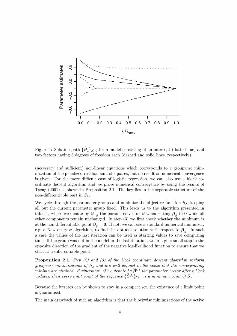
The best model with respect to the log-likelihood score on the validation set is theGroup Lasso estimator. It is followed by the Group Lasso/Ridge hybrid and the GroupLasso/MLE hybrid. The corresponding values of ρmax on the test set are 0.6593, 0.6569and 0.6541, respectively. They are all competitive with the results from Yeo and Burge(2004) whose best ρmax equals 0.6589. While the Group Lasso solution has some active3-way interactions, the Group Lasso/Ridge hybrid and the Group Lasso/MLE hybrid onlycontain 2-way interactions. Figure 3 shows the `2-norm of each parameter group for thethree estimators. The 3-way interactions of the Group Lasso solution seem to be very weak.Considering also the non-hierarchical models for the two-stage procedures yields the sameselected terms. Decreasing the candidate model size to only contain 2-way interactionsgives similar results.

In summary, the prediction performance of the Group Lasso and its variants is competitivewith the Maximum Entropy models used in Yeo and Burge (2004) which have been viewedas (among) the best for short motif modeling and splice site prediction. Advantagesof the Group Lasso and variants thereof include selection of terms. In addition, other(possibly continuous) predictor variables as for example global sequence information couldbe naturally included in the Group Lasso approach to improve the rather low correlationcoefficients (Yeo and Burge, 2004).

6 Discussion

We study the Group Lasso for logistic regression. We present efficient algorithms, espe-cially suitable for high-dimensional problems, for solving the corresponding convex opti-mization problem which is inherently more difficult than `1-penalized logistic regression.The algorithms rely on recent theory and developments for block coordinate and block co-ordinate gradient descent (Tseng, 2001; Tseng and Yun, 2006) and we give rigorous proofsthat our algorithms yield a solution of the corresponding convex optimization problem. Incontrast to the algorithm in Kim et al. (2006), our procedure is fully automatic and doesnot require the specification of an algorithmic tuning parameter. Moreover, our algorithm

16

Term

1 3 5 7 1:3 1:5 1:7 2:4 2:6 3:4 3:6 4:5 4:7 5:72 4 6 1:2 1:4 1:6 2:3 2:5 2:7 3:5 3:7 4:6 5:6 6:7

l 2−n

orm

01

2 GLGL/RGL/MLE

Term

1:2:3 1:2:5 1:2:7 1:3:5 1:3:7 1:4:6 1:5:6 1:6:7 2:3:5 2:3:7 2:4:6 2:5:6 2:6:7 3:4:6 3:5:6 3:6:7 4:5:7 5:6:71:2:4 1:2:6 1:3:4 1:3:6 1:4:5 1:4:7 1:5:7 2:3:4 2:3:6 2:4:5 2:4:7 2:5:7 3:4:5 3:4:7 3:5:7 4:5:6 4:6:7

l 2−n

orm

01

2

Figure 3: `2-norms ‖βg‖2, g ∈ {1, . . . , G} of the parameter groups with respect to theblockwise orthonormalized design matrix when using a candidate model with all 3-wayinteractions. i : j : k denotes the 3-way interaction between the ith, jth and kth sequenceposition. The same scheme applies to the 2-way interactions and the main effects. Active3-way interactions are additionally marked with vertical lines.

is much faster than the recent proposal from Park and Hastie (2006b). Additionally, wepresent a statistical consistency theory for the setting where the predictor dimension ispotentially much larger than sample size but assuming the true underlying logistic re-gression model is sparse. The algorithms with the supporting mathematical optimizationtheory as well as the statistical consistency theory also apply directly to the Group Lassoin other generalized linear models.

Furthermore, we propose the Group Lasso/Ridge hybrid method which often yields betterpredictions and better variable selection than the Group Lasso. In addition, our GroupLasso/Ridge hybrid allows for hierarchical model fitting which has not been developed yetfor `1-penalization or the Group Lasso.

Finally, we apply the Group Lasso and its variants to short DNA motif modeling andsplice site detection. Our general methodology performs very well in comparison to themaximum entropy method which is considered to be among the best for this task.

17

Acknowledgement

We would like to thank Sylvain Sardy for helpful comments.

18

A Appendix

A.1 Proof of Lemma 2.1

We will first eliminate the intercept. Let β1, . . . ,βg be fixed. To get the estimate for theintercept we have to minimize a function of the form

g(β0) = −

n∑

i=1

[yi(β0 + ci)− log(1 + exp{β0 + ci})]

with derivative

g′(β0) = −n∑

i=1

[yi −

exp{β0 + ci}

1 + exp{β0 + ci}

],

where ci =∑G

g=1 xTi,gβg is a constant. It holds that limβ0→∞ g′(β0) = n −

∑ni=1 yi >

0 and limβ0→−∞ g′(β0) = −∑n

i=1 yi < 0. Furthermore g′(·) is continuous and strictlyincreasing. Therefore there exists a unique β∗

0 ∈ R such that g′(β∗0) = 0. By the implicit

function theorem the corresponding function β∗0(β1, . . . ,βG) is continuously differentiable.

By replacing β0 in Sλ(β) by the function β∗0(β1, . . . ,βG) and using duality theory, we can

rewrite (2.2) as an optimization problem under the constraint∑G

g=1 ‖βg‖2 ≤ t for somet > 0. This is an optimization problem of a continuous function over a compact set, hencethe minimum is attained.

A.2 Proof of Proposition 2.1

We first show that the groupwise minima of Sλ are attained. For g = 0 this follows fromthe proof of Lemma 2.1. The case g ≥ 1 corresponds to a minimization of a continuousfunction over a compact set, hence the minimum is attained. We now show that step (3)minimizes the convex function Sλ(βg) for g ≥ 1. The subdifferential of Sλ with respect

to βg is the set ∂Sλ(βg) = {−XTg (y − pβ) + λe, e ∈ E(βg)}, E(βg) = {e ∈ R

dfg : eg =

s(dfg)βg

‖βg‖2if βg 6= 0 and s(dfg)‖eg‖2 ≤ 1 if βg = 0}. By using subdifferential calculus

we know that βg minimizes Sλ(βg) if and only if 0 ∈ ∂Sλ(βg) which is equivalent to theformulation of step 3. Furthermore conditions (A1), (B1) - (B3) and (C2) in Tseng (2001)hold. By Lemma 3.1 and Proposition 5.1 in Tseng (2001) every limit point of the sequence{β(t)}t≥0 is a stationary point of the convex function Sλ, hence a minimum point.

A.3 Proof of Proposition 2.2

The proposition directly follows from Theorem 4.1(e) of Tseng and Yun (2006). We haveto show that −H (t) is bounded by above and away from zero. The Hessian of the negativelog-likelihood function is N =

∑ni=1 pβ(xi)(1 − pβ(xi))xix

Ti �

14XT X in the sense that

N − 14XT X is negative semidefinite. For the blockmatrix Ngg corresponding to the gth

predictor it follows from the blockwise orthonormalization that Ngg �n4 Idfg

and hence

max{diag(Ngg)} ≤n4 . An upper bound on −H (t) is therefore always guaranteed. The

lower bound is enforced by the choice of H(t)gg . By the choice of the line search we ensure

that α(t) is bounded by above and therefore Theorem 4.1(e) of Tseng and Yun (2006) canbe applied.

19

A.4 Outline of the Proof of the Consistency Result

The proof follows the arguments used in Tarigan and van de Geer (2006). The latterconsider hinge loss instead of logistic loss, but, as they point out, a large part of theirresults can be easily extended because only the Lipschitz property of the loss is usedthere. Furthermore, under (A1), logistic loss has the usual “quadratic” behaviour nearits overal minimum. This means that it does not share the problem of unknown marginbehaviour with hinge loss, i.e. the situation is in that respect simpler than in Tarigan andvan de Geer (2006).

The Group Lasso reduces to the `1 penalty (the usual Lasso) when there is only onedegree of freedom in each group. The extension of consistency results to more degrees offreedom is straightforward, provided maxg dfg does not depend on n. We furthermore notethat the Group Lasso uses a normalization involving the design matrix of the observedpredictors. For the consistency result, one needs to prove that this empirical normalizationis uniformly close to the theoretical one. This boils down to showing that empirical andtheoretical eigenvalues of the design matrix per group cannot be too far away from eachother, uniformly over the groups. Here, we invoke that assumption (A4) implies that L2

n

is no larger than c1/(C1 log G). We then apply (A3) in Bernstein’s inequality to boundthe difference in eigenvalues.

A technical extension as compared to Tarigan and van de Geer (2006) is that we do notassume an a priori bound on the functions ηβ(·). This is now handled by using convexityarguments (similar to van de Geer (2003)), and again part of the assumption (A4), namelythat λ is smaller than c1/((1+N0)

2L2n). This assumption ensures that for all n, with high

probability, the difference between ηβ0 and the estimated regression ηbβλis bounded by a

constant independent of n.

20

References

Bakin, S. (1999) Adaptive Regression and Model Selection in Data Mining Problems. Ph.D.thesis, Australian National University.

Balakrishnan, S. and Madigan, D. (2006) Algorithms for sparse linear classifiers in the mas-sive data setting. Available at http://www.stat.rutgers.edu/~madigan/PAPERS/.

Bertsekas, D. P. (2003) Nonlinear Programming. Athena Scientific.

Burge, C. (1998) Modeling dependencies in pre-mrna splicing signals. In ComputatationalMethods in Molecular Biology (eds. S. Salzberg, D. Searls and S. Kasif), chap. 8, 129–164. Elsevier Science.

Burge, C. and Karlin, S. (1997) Prediction of complete gene structures in human genomicdna. Journal of Molecular Biology, 268, 78–94.

Efron, B., Hastie, T., Johnstone, I. and Tibshirani, R. (2004) Least angle regression. TheAnnals of Statistics, 32, 407–499.

Genkin, A., Lewis, D. D. and Madigan, D. (2004) Large-scale bayesian logistic regres-sion for text categorization. Available at http://www.stat.rutgers.edu/~madigan/

PAPERS/.

Kim, Y., Kim, J. and Kim, Y. (2006) Blockwise sparse regression. Statistica Sinica, 16.

King, G. and Zeng, L. (2001) Logistic regression in rare events data. Political Analysis,9, 137–163.

Krishnapuram, B., Carin, L., Figueiredo, M. A. and Hartemink, A. J. (2005) Sparse multi-nomial logistic regression: Fast algorithms and generalization bounds. IEEE Transac-tions on Pattern Analysis and Machine Intelligence, 27, 957–968.

Lokhorst, J. (1999) The lasso and generalised linear models. Honors Project, The Univer-sity of Adelaide, Australia.

Meinshausen, N. (2007) Lasso with relaxation. Computational Statistics and Data Anal-ysis. To appear.

Osborne, M., Presnell, B. and Turlach, B. (2000) A new approach to variable selection inleast squares problems. IMA Journal of Numerical Analysis, 20, 389–403.

Park, M.-Y. and Hastie, T. (2006a) An l1 regularization-path algorithm for generalizedlinear models. Available at http://www-stat.stanford.edu/~hastie/pub.htm.

Park, M.-Y. and Hastie, T. (2006b) Regularization path algorithms for detecting geneinteractions. Available at http://www-stat.stanford.edu/~hastie/pub.htm.

Rosset, S. (2005) Following curved regularized optimization solution paths. In Advancesin Neural Information Processing Systems 17 (eds. L. K. Saul, Y. Weiss and L. Bottou),1153–1160. Cambridge, MA: MIT Press.

Tarigan, B. and van de Geer, S. (2006) Classifiers of support vector machine type, with`1 penalty. Bernoulli. To appear.

21

Tibshirani, R. (1996) Regression shrinkage and selection via the lasso. Journal of theRoyal Statistical Society Series B, 58, 267–288.

Tibshirani, R. (1997) The lasso method for variable selection in the cox model. Statisticsin Medicine, 16, 385–395.

Tseng, P. (2001) Convergence of a block coordinate descent method for nondifferentiableminimization. Journal of Optimization Theory and Applications, 109, 475–494.

Tseng, P. and Yun, S. (2006) A coordinate gradient descent method for nonsmooth sepa-rable minimization. Preprint.

van de Geer, S. (2003) Adaptive quantile regression. In Recent Advances and Trends inNonparametric Statistics (eds. M. Akritas and D. Politis), 235–250. Elsevier.

Yeo, G. W. and Burge, C. B. (2004) Maximum entropy modeling of short sequence motifswith applications to rna splicing signals. Journal of Computational Biology, 11, 475–494.

Yuan, M. and Lin, Y. (2006) Model selection and estimation in regression with groupedvariables. Journal of the Royal Statistical Society Series B, 68, 49–67.

Zhao, P. and Yu, B. (2004) Boosted lasso. Tech. rep., University of California, Berkeley.

22