The Grossone methodology perspective on Turing machines · 2015-01-29 · A new perspective on...

The Grossone methodology perspective onTuring machines

Yaroslav D. Sergeyev and Alfredo Garro

Abstract This chapter discusses how the mathematical language used to describeand to observe automatic computations influences the accuracy of the obtainedresults. The chapter presents results obtained by describing and observing dif-ferent kinds of Turing machines (single and multi-tape, deterministic and non-deterministic) through the lens of a new mathematical language named Grossone.This emerging language is strongly based on three methodological ideas borrowedfrom Physics and applied to Mathematics: the distinction between the object (indeedmathematical object) of an observation and the instrument used for this observation;interrelations holding between the object and the tool usedfor the observation; theaccuracy of the observation determined by the tool. In the chapter, the new resultsare compared to those achievable by using traditional languages. It is shown thatboth languages do not contradict each other but observe and describe the same ob-ject (Turing machines) but with different accuracies.

1 Introduction

Turing machines represent one of the simple abstract computational devices that canbe used to investigate the limits of computability . In this chapter, they are consid-ered from several points of view that emphasize the importance and the relativity of

Yaroslav D. SergeyevDipartimento di Ingegneria Informatica, Modellistica, Elettronica e Sistemistica (DIMES), Uni-versita della Calabria, Rende (CS), Italy.N.I. Lobatchevsky State University, Nizhni Novgorod, Russia.Istituto di Calcolo e Reti ad Alte Prestazioni, C.N.R., Rende (CS), Italy.e-mail: [email protected]

Alfredo GarroDipartimento di Ingegneria Informatica, Modellistica, Elettronica e Sistemistica (DIMES), Uni-versita della Calabria, Rende (CS), Italy.e-mail: [email protected]

1

2 Yaroslav D. Sergeyev and Alfredo Garro

mathematical languages used to describe the Turing machines. A deep investigationis performed on the interrelations between mechanical computations and their math-ematical descriptions emerging when a human (the researcher) starts to describe aTuring machine (the object of the study) by different mathematical languages (theinstruments of investigation).

In particular, we focus our attention on different kinds of Turing machines (singleand multi-tape, deterministic and non-deterministic) by organizing and discussingthe results presented in [42] and [43] so to provide a compendium of our multi-yearresearch on this subject.

The starting point is represented by numeral systems1 that we use to write downnumbers, functions, models, etc. and that are among our tools of investigation ofmathematical and physical objects. It is shown that numeralsystems strongly in-fluence our capabilities to describe both the mathematical and physical worlds. Anew numeral system introduced in [30, 32, 37]) for performing computations withinfinite and infinitesimal quantities is used for the observation of mathematical ob-jects and studying Turing machines. The new methodology is based on the principle‘The part is less than the whole’ introduced by Ancient Greeks (see, e.g., Euclid’sCommon Notion 5) and observed in practice. It is applied to all sets and processes(finite and infinite) and all numbers (finite, infinite, and infinitesimal).

In order to see the place of the new approach in the historicalpanorama of ideasdealing with infinite and infinitesimal, see [19, 20, 21, 35, 36, 42, 43]. The newmethodology has been successfully applied for studying a number of applications:percolation (see [13, 45]), Euclidean and hyperbolic geometry (see [22, 29]), fractals(see [31, 33, 40, 45]), numerical differentiation and optimization (see [7, 34, 38,48]), ordinary differential equations (see [41]), infiniteseries (see [35, 39, 47]), thefirst Hilbert problem (see [36]), and cellular automata (see[8]).

The rest of the chapter is structured as follows. In Section 2, Single and Multi-tape Turing machines are introduced along with “classical”results concerning theircomputational power and related equivalences; in Section 3a brief introduction tothe new language and methodology is given whereas their exploitation for analyzingand observing the different types of Turing machines is discussed in Section 4. Itshows that the new approach allows us to observe Turing machines with a higheraccuracy giving so the possibility to better characterize and distinguish machineswhich are equivalent when observed within the classical framework. Finally, Sec-tion 5 concludes the chapter.

1 We are reminded that anumeralis a symbol or group of symbols that represents anumber. Thedifference between numerals and numbers is the same as the difference between words and thethings they refer to. Anumberis a concept that anumeralexpresses. The same number can berepresented by different numerals. For example, the symbols ‘7’, ‘seven’, and ‘VII’ are differentnumerals, but they all represent the same number.

A new perspective on Turing machines 3

2 Turing machines

The Turing machine is one of the simple abstract computational devices that can beused to model computational processes and investigate the limits of computability.In the following subsections, deterministic Single and Multi-tape Turing machinesare described along with important classical results concerning their computationalpower and related equivalences (see Section 2.1 and 2.2 respectively); finally, non-deterministic Turing machines are introduced (see Section2.3).

2.1 Single-Tape Turing machines

A Turing machine (see, e.g., [12, 44]) can be defined as a 7-tuple

M =⟨Q,Γ, b,Σ,q0,F,δ

⟩, (1)

whereQ is a finite and not empty set of states;Γ is a finite set of symbols;b∈ Γ isa symbol called blank;Σ ⊆ {Γ− b} is the set of input/output symbols;q0 ∈ Q is theinitial state;F ⊆ Q is the set of final states;δ : {Q−F}×Γ 7→ Q×Γ×{R,L,N} isa partial function called the transition function, whereL means left,R means right,andN means no move .

Specifically, the machine is supplied with: (i) ataperunning through it which isdivided into cells each capable of containing a symbolγ ∈ Γ, whereΓ is called thetape alphabet, andb∈ Γ is the only symbol allowed to occur on the tape infinitelyoften; (ii) aheadthat can read and write symbols on the tape and move the tape leftand right one and only one cell at a time. The behavior of the machine is specifiedby its transition functionδ and consists of a sequence of computational steps ; ineach step the machine reads the symbol under the head and applies thetransitionfunctionthat, given the current state of the machine and the symbol itis reading onthe tape, specifies (if it is defined for these inputs): (i) thesymbolγ ∈ Γ to write onthe cell of the tape under the head; (ii) the move of the tape (L for one cell left,R forone cell right,N for no move); (iii) the next stateq∈ Q of the machine.

2.1.1 Classical results for Single-Tape Turing machines

Starting from the definition of Turing machine introduced above, classical results(see, e.g., [1]) aim at showing that different machines in terms of provided tape andalphabet have the same computational power, i.e., they are able to execute the samecomputations. In particular, two main results are reportedbelow in an informal way.

Given a Turing machineM = {Q,Γ, b,Σ,q0,F,δ}, which is supplied with an infi-nite tape, it is always possible to define a Turing machineM ′= {Q′,Γ′, b,Σ′,q′0,F

′,δ′}which is supplied with a semi-infinite tape (e.g., a tape witha left boundary) and isequivalent toM , i.e., is able to execute all the computations ofM .


Given a Turing machineM = {Q,Γ, b,Σ,q0,F,δ}, it is always possible to definea Turing machineM ′ = {Q′,Γ′, b,Σ′,q′0,F

′,δ′} with |Σ′| = 1 andΓ′ = Σ′ ∪ {b},which is equivalent toM , i.e., is able to execute all the computations ofM .

It should be mentioned that these results, together with theusual conclusion re-garding the equivalences of Turing machines, can be interpreted in the following,less obvious, way: they show that when we observe Turing machines by exploitingthe classical framework we are not able to distinguish, fromthe computational pointof view, Turing machines which are provided with alphabets having different num-ber of symbols and/or different kind of tapes (infinite or semi-infinite) (see [42] fora detailed discussion).

2.2 Multi-tape Turing machines

Let us consider a variant of the Turing machine defined in (1) where a machineis equipped with multiple tapes that can be simultaneously accessed and updatedthrough multiple heads (one per tape). These machines can beused for a more directand intuitive resolution of different kind of computational problems. As an example,in checking if a string is palindrome it can be useful to have two tapes on whichrepresent the input string so that the verification can be efficiently performed byreading a tape from left to right and the other one from right to left.

Moving towards a more formal definition, ak-tapes,k ≥ 2, Turing machine(see [12]) can be defined (cf. (1)) as a 7-tuple

M K =⟨

Q,Γ, b,Σ,q0,F,δ(k)⟩, (2)

whereΣ =⋃k

i=1 Σi is given by the union of the symbols in the k input/output al-phabetsΣ1, . . . ,Σk; Γ = Σ∪{b} whereb is a symbol called blank;Q is a finite andnot empty set of states;q0 ∈ Q is the initial state;F ⊆ Q is the set of final states;δ(k) : {Q−F}×Γ1 × ·· · ×Γk 7→ Q×Γ1 × ·· · ×Γk ×{R,L,N}k is a partial func-tion called the transition function, whereΓi = Σi ∪{b}, i = 1, . . . ,k, L means left,Rmeans right, andN means no move .

This definition ofδ(k) means that the machine executes a transition starting froman internal stateqi and with thek heads (one for each tape) above the charactersai1, . . . ,ai k, i.e., if δ(k)(q1,ai1, . . . ,ai k) = (q j ,a j 1, . . . ,a j k,zj 1, . . . ,zj k) the machinegoes in the new stateq j , write on the k tapes the charactersa j 1, . . . ,a j k respec-tively, and moves each of its k heads left, right or no move, asspecified by thezj l ∈ {R,L,N}, l = 1, . . . ,k.

A machine can adopt for each tape a different alphabet, in anycase, for each tape,as for the Single-tape Turing machines, the minimum portioncontaining charactersdistinct fromb is usually represented. In general, a typical configurationof a Multi-tape machine consists of a read-only input tape, several read and write work tapes,and a write-only output tape, with the input and output tapesaccessible only in onedirection. In the case of ak-tapes machine, the instant configuration of the machine,


as for the Single-tape case, must describe the internal state, the contents of the tapesand the positions of the heads of the machine.

More formally, for ak-tapes Turing machineM K =⟨

Q,Γ, b,Σ,q0,F,δ(k)⟩

with

Σ =⋃k

i=1 Σi (see 2) a configuration of the machine is given by:

q#α1 ↑ β1#α2 ↑ β2#. . .#αk ↑ βk, (3)

whereq∈ Q; αi ∈ ΣiΓ∗i ∪{ε} andβi ∈ Γ∗

i Σi ∪{b}. A configuration isfinal if q∈ F .Thestartingconfiguration usually requires the input stringx on a tape, e.g., the

first tape so thatx∈ Σ∗1, and onlyb symbols on all the other tapes. However, it can be

useful to assume that, at the beginning of a computation, these tapes have a startingsymbolZ0 /∈ Γ =

⋃ki=1 Γi . Therefore, in the initial configuration the head on the first

tape will be on the first character of the input stringx, whereas the heads on the othertapes will observe the symbolZ0, more formally, by re-placingΓi = Σi ∪{b,Z0} inall the previous definition, a configurationq#α1 ↑ β1#α2 ↑ β2#. . .#αk ↑ βk is aninitial configurationif αi = ε, i = 1, . . . ,k,β1 ∈ Σ∗

1,βi = Z0, i = 2, . . . ,k andq= q0.The application of the transition functionδ(k) at a machine configuration (c.f.

(3)) defines acomputational stepof a Multi-tape Turing machine . The set of com-putational steps which bring the machine from the initial configuration into a finalconfiguration defines thecomputationexecuted by the machine. As an example,the computation of a Multi-tape Turing machineM K which computes the functionfMK

(x) can be represented as follows:

q0# ↑ x# ↑ Z0#. . .# ↑ Z0

→M K q# ↑ x# ↑ fMK

(x)# ↑ b#. . .# ↑ b (4)

whereq∈ F and→M K indicates the transition among machine configurations.

2.2.1 Classical results for Multi-Tape Turing machines

It is worth noting that, although thek-tapes Turing machine can be used for a moredirect resolution of different kind of computational problems, in the classical frame-work it has the same computational power of the Single-tape Turing machine. Moreformally, given a Multi-tape Turing machine it is always possible to define a Single-tape Turing machine which is able to fully simulate its behavior and therefore tocompletely execute its computations. In particular, the Single-tape Turing machinesadopted for the simulation use a particular kind of the tape which is divided intotracks (multi-track tape). In this way, if the tape hasm tracks, the head is able toaccess (for reading and/or writing) all them characters on the tracks during a sin-gle operation. If for them tracks the alphabetsΓ1, . . . Γm are adopted respectively,the machine alphabetΓ is such that|Γ| = |Γ1×·· ·×Γm| and can be defined by aninjective function from the setΓ1 × ·· · ×Γm to the setΓ; this function will asso-ciate the symbolb in Γ to the tuple(b, b, . . . , b) in Γ1 × ·· · ×Γm. In general, the


elements ofΓ which correspond to the elements inΓ1× ·· ·×Γm can be indicatedby [ai1,ai2, . . . ,aim] whereai j ∈ Γ j .

By adopting this notation it is possible to demonstrate thatgiven ak-tapes TuringmachineM K = {Q,Γ, b,Σ,q0,F,δ(k)} it is always possible to define a Single-tapeTuring machine which is able to simulatet computational steps ofM K = in O(t2)transitions by using an alphabet withO((2|Γ|)k) symbols (see [1]) .

The proof is based on the definition of a machineM ′ = {Q′,Γ′, b,Σ′,q′0,F′,δ′}

with a Single-tape divided into 2k tracks (see [1]);k tracks for storing the charactersin thek tapes ofM K andk tracks for signing through the marker↓ the positions ofthek heads on thek tapes ofM k. As an example, this kind of tape can represent thecontent of each tapes ofM k and the position of each machine heads in its even andodd tracks respectively. As discussed above, for obtaininga Single-tape machineable to represent these 2k tracks, it is sufficient to adopt an alphabet with the requiredcardinality and define an injective function which associates a 2k-ple characters ofa cell of the multi-track tape to a symbols in this alphabet.

The transition functionδ(k) of thek-tapes machine is given byδ(k)(q1,ai1, . . . ,ai k)=(q j ,a j 1, . . . ,a j k,zj 1, . . . ,zj k), with zj 1, . . . ,zj k ∈ {R,L,N}; as a consequence the cor-responding transition functionδ′ of the Single-tape machine, for each transitionspecified byδ(k) must individuate the current state and the position of the markerfor each track and then write on the tracks the required symbols, move the markersand go in another internal state. For each computational step of M K , the machineM ′ must execute a sequence of steps for covering the portion of tapes between thetwo most distant markers. As in each computational step a marker can move at mostof one cell and then two markers can move away each other at most of two cells,aftert steps ofM K the markers can be at most 2t cells distant, thus ifM K executest steps,M ′ executes at most: 2∑t

i=1 i = t2+ t = O(t2) steps .Moving to the cost of the simulation in terms of the number of required characters

for the alphabet of the Single-tape machine, we recall that|Γ1| = |Σ1|+1 and that|Γi | = |Σi |+2 for 2≤ i ≤ k. So by multiplying the cardinalities of these alphabetswe obtain that:|Γ′|= 2k(|Σ1|+1)∏k

i=2(|Σi |+2) = O((2max1≤i≤k |Γi |)k).

2.3 Non-deterministic Turing machines

A non-deterministic Turing machine (see [12]) can be defined(cf. (1)) as a 7-tuple

MN =⟨Q,Γ, b,Σ,q0,F,δN

⟩, (5)

whereQ is a finite and not empty set of states;Γ is a finite set of symbols;b∈ Γ isa symbol called blank;Σ ⊆ {Γ− b} is the set of input/output symbols;q0 ∈ Q is theinitial state;F ⊆Q is the set of final states;δN : {Q−F}×Γ 7→ P (Q×Γ×{R,L,N})is a partial function called the transition function, whereL means left,Rmeans right,andN means no move .


As for a deterministic Turing machine (see (1)), the behavior of MN is specifiedby its transition functionδN and consists of a sequence of computational steps . Ineach step, given the current state of the machine and the symbol it is reading onthe tape, the transition functionδN returns (if it is defined for these inputs) a set oftriplets each of which specifies: (i) a symbolγ ∈ Γ to write on the cell of the tapeunder the head; (ii) the move of the tape (L for one cell left,R for one cell right,Nfor no move); (iii) the next stateq∈ Q of the Machine. Thus, in each computationalstep, the machine cannon-deterministicallyexecute different computations, one foreach triple returned by the transition function.

An important characteristic of a non-deterministic Turingmachine (see, e.g., [1])is its non-deterministic degree

d = ν(MN) = maxq∈Q−F,γ∈Γ

|δN(q,γ)|

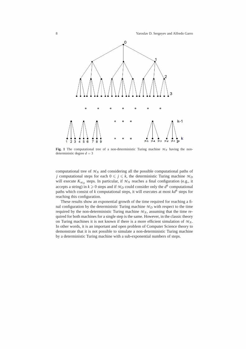
defined as the maximal number of different configurations reachable in a singlecomputational step starting from a given configuration. Thebehavior of the machinecan be then represented as a tree whose branches are the computations that themachine can execute starting from the initial configurationrepresented by the node0 and nodes of the tree at the levels 1, 2, etc. represent subsequent configurations ofthe machine.

Let us consider an example shown in Fig. 1 where a non-deterministic machineMN having the non-deterministic degreed = 3 is presented. The depth of the com-putational tree is equal tok. In this example, it is supposed that the computationaltree ofMN is complete (i.e., each node has exactlyd children). Then, obviously, thecomputational tree ofMN hasdk = 3k leaf nodes.

2.3.1 Classical results for non-deterministic Turing machines

An important result for the classic theory on Turing machines (see e.g., [1]) is thatfor any non-deterministic Turing machineMN there exists an equivalent determinis-tic Turing machineMD. Moreover, if the depth of the computational tree generatedby MN is equal tok, then for simulatingMN, the deterministic machineMD willexecute at most

KMD=

k

∑j=0

jd j = O(kdk)

computational steps.Intuitively, for simulatingMN, the deterministic Turing machineMD executes

a breadth-first visit of the computational tree ofMN. If we consider the examplefrom Fig. 1 withk = 3, then the computational tree ofMN hasdk = 27 leaf nodesanddk = 27 computational paths consisting ofk = 3 branches (i.e., computationalsteps) . Then, the tree containsdk−1 = 9 computational paths consisting ofk−1= 2branches anddk−2 = 3 computational paths consisting ofk−2= 1 branches . Thus,for simulating all the possible computations ofMN, i.e., for complete visiting the


Fig. 1 The computational tree of a non-deterministic Turing machineMN having the non-deterministic degreed = 3

computational tree ofMN and considering all the possible computational paths ofj computational steps for each 06 j 6 k, the deterministic Turing machineMD

will executeKMDsteps. In particular, ifMN reaches a final configuration (e.g., it

accepts a string) ink> 0 steps and ifMD could consider only thedk computationalpaths which consist ofk computational steps, it will executes at mostkdk steps forreaching this configuration.

These results show an exponential growth of the time required for reaching a fi-nal configuration by the deterministic Turing machineMD with respect to the timerequired by the non-deterministic Turing machineMN, assuming that the time re-quired for both machines for a single step is the same. However, in the classic theoryon Turing machines it is not known if there is a more efficient simulation ofMN.In other words, it is an important and open problem of Computer Science theory todemonstrate that it is not possible to simulate a non-deterministic Turing machineby a deterministic Turing machine with a sub-exponential numbers of steps.


3 The Grossone Language and Methodology

In this section, we give just a brief introduction to the methodology of the newapproach [30, 32] dwelling only on the issues directly related to the subject of thechapter. This methodology will be used in Section 4 to study Turing machines andto obtain some more accurate results with respect to those obtainable by using thetraditional framework [4, 44] .

In order to start, let us remind that numerous trials have been done duringthe centuries to evolve existing numeral systems in such a way that numeralsrepresenting infinite and infinitesimal numbers could be included in them (see[2, 3, 5, 17, 18, 25, 28, 46]). Since new numeral systems appear very rarely, in eachconcrete historical period their significance for Mathematics is very often underes-timated (especially by pure mathematicians). In order to illustrate their importance,let us remind the Roman numeral system that does not allow oneto express zero andnegative numbers. In this system, the expression III-X is anindeterminate form. Asa result, before appearing the positional numeral system and inventing zero math-ematicians were not able to create theorems involving zero and negative numbersand to execute computations with them.

There exist numeral systems that are even weaker than the Roman one. They se-riously limit their users in executing computations. Let usrecall a study publishedrecently inScience(see [11]). It describes a primitive tribe living in Amazonia (Pi-raha). These people use a very simple numeral system for counting: one, two, many.For Piraha, all quantities larger than two are just ‘many’ and such operations as 2+2and 2+1 give the same result, i.e., ‘many’. Using their weak numeral system Pirahaare not able to see, for instance, numbers 3, 4, 5, and 6, to execute arithmetical op-erations with them, and, in general, to say anything about these numbers because intheir language there are neither words nor concepts for that.

In the context of the present chapter, it is very important that the weakness ofPiraha’s numeral system leads them to such results as

‘many’+1= ‘many’, ‘many’+2= ‘many’, (6)

which are very familiar to us in the context of views on infinity used in the traditionalcalculus

∞+1= ∞, ∞+2= ∞. (7)

The arithmetic of Piraha involving the numeral ‘many’ has also a clear similaritywith the arithmetic proposed by Cantor for his Alephs2:

ℵ0+1= ℵ0, ℵ0+2= ℵ0, ℵ1+1= ℵ1, ℵ1+2= ℵ1. (8)

2 This similarity becomes even more pronounced if one considers another Amazonian tribe –Munduruku (see [26]) – who fail in exact arithmetic with numbers larger than 5 but are able tocompare and add large approximate numbers that are far beyond their naming range. Particularly,they use the words ‘some, not many’ and ‘many, really many’ to distinguish two types of largenumbers using the rules that are very similar to ones used by Cantorto operate withℵ0 andℵ1,respectively.


Thus, the modern mathematical numeral systems allow us to distinguish a largerquantity of finite numbers with respect to Piraha but give results that are similar tothose of Piraha when we speak about infinite quantities. This observation leads us tothe following idea:Probably our difficulties in working with infinity is not connectedto the nature of infinity itself but is a result of inadequate numeral systems that weuse to work with infinity, more precisely, to express infinitenumbers.

The approach developed in [30, 32, 37] proposes a numeral system that usesthe same numerals for several different purposes for dealing with infinities and in-finitesimals: in Analysis for working with functions that can assume different infi-nite, finite, and infinitesimal values (functions can also have derivatives assumingdifferent infinite or infinitesimal values); for measuring infinite sets; for indicatingpositions of elements in ordered infinite sequences ; in probability theory, etc. (see[7, 8, 13, 22, 29, 31, 33, 34, 35, 36, 38, 39, 40, 45, 47, 48]). Itis important to em-phasize that the new numeral system avoids situations of thetype (6)–(8) providingresults ensuring that ifa is a numeral written in this system then for anya (i.e., acan be finite, infinite, or infinitesimal) it followsa+1> a.

The new numeral system works as follows. A new infinite unit ofmeasure ex-pressed by the numeral① calledgrossoneis introduced as the number of elementsof the set,N, of natural numbers. Concurrently with the introduction ofgrossone inthe mathematical language all other symbols (like∞, Cantor’sω, ℵ0,ℵ1, ..., etc.)traditionally used to deal with infinities and infinitesimals are excluded from the lan-guage because grossone and other numbers constructed with its help not only canbe used instead of all of them but can be used with a higher accuracy3. Grossone isintroduced by describing its properties postulated by the Infinite Unit Axiom (see[32, 37]) added to axioms for real numbers (similarly, in order to pass from the set,N, of natural numbers to the set,Z, of integers a new element – zero expressed bythe numeral 0 – is introduced by describing its properties) .

The new numeral① allows us to construct different numerals expressing differentinfinite and infinitesimal numbers and to execute computations with them. Let usgive some examples. For instance, in Analysis, indeterminate forms are not presentand, for example, the following relations hold for① and①−1 (that is infinitesimal),as for any other (finite, infinite, or infinitesimal) number expressible in the newnumeral system

0·① = ① ·0= 0, ①−① = 0,①

①= 1, ①0 = 1, 1① = 1, 0① = 0, (9)

0·①−1 = ①−1 ·0= 0, ①−1 > 0, ①−2 > 0, ①−1−①−1 = 0, (10)

①−1

①−1 = 1,①−2

①−2 = 1, (①−1)0 = 1, ① ·①−1 = 1, ① ·①−2 = ①−1. (11)

The new approach gives the possibility to develop a new Analysis (see [35])where functions assuming not only finite values but also infinite and infinitesimal

3 Analogously, when the switch from Roman numerals to the Arabic ones has been done, numeralsX, V, I, etc. have been excluded from records using Arabic numerals.


ones can be studied. For all of them it becomes possible to introduce a new notionof continuity that is closer to our modern physical knowledge. Functions assumingfinite and infinite values can be differentiated and integrated.

By using the new numeral system it becomes possible to measure certain infinitesets and to see, e.g., that the sets of even and odd numbers have ①/2 elementseach. The set,Z, of integers has 2①+1 elements (① positive elements,① negativeelements, and zero). Within the countable sets and sets having cardinality of thecontinuum (see [20, 36, 37]) it becomes possible to distinguish infinite sets havingdifferent number of elements expressible in the numeral system using grossone andto see that, for instance,

①

2< ①−1< ① < ①+1< 2①+1< 2①2−1< 2①2 < 2①2+1<

2①2+2< 2①−1< 2① < 2①+1< 10① < ①①−1< ①① < ①①+1. (12)

Another key notion for our study of Turing machines is that ofinfinite sequence.Thus, before considering the notion of the Turing machine from the point of viewof the new methodology, let us explain how the notion of the infinite sequence canbe viewed from the new positions.

3.1 Infinite sequences

Traditionally, aninfinite sequence{an},an ∈ A, n∈ N, is defined as a function hav-ing the set of natural numbers,N, as the domain and a setA as the codomain. Asubsequence{bn} is defined as a sequence{an} from which some of its elementshave been removed . In spite of the fact that the removal of theelements from{an}can be directly observed, the traditional approach does notallow one to register, inthe case where the obtained subsequence{bn} is infinite, the fact that{bn} has lesselements than the original infinite sequence{an}.

Let us study what happens when the new approach is used. From the point ofview of the new methodology, an infinite sequence can be considered in a dual way:either as an object of a mathematical study or as a mathematical instrument devel-oped by human beings to observe other objects and processes.First, let us considerit as a mathematical object and show that the definition of infinite sequences shouldbe done more precise within the new methodology. In the finitecase, a sequencea1,a2, . . . ,an hasn elements and we extend this definition directly to the infinitecase saying that an infinite sequencea1,a2, . . . ,an hasn elements wheren is ex-pressed by an infinite numeral such that the operations with it satisfy the Postulate 3of the Grossone methodology4. Then the following result (see [30, 32]) holds. Wereproduce here its proof for the sake of completeness.

4 The Postulate 3 states:The part is less than the wholeis applied to all numbers (finite, infinite,and infinitesimal) and to all sets and processes (finite and infinite), see[30].


Theorem 1. The number of elements of any infinite sequence is less or equal to ①.

Proof. The new numeral system allows us to express the number of elementsof the setN as①. Thus, due to the sequence definition given above, any sequencehavingN as the domain has① elements.

The notion of subsequence is introduced as a sequence from which some of itselements have been removed. This means that the resulting subsequence will haveless elements than the original sequence. Thus, we obtain infinite sequences havingthe number of members less than grossone. 2

It becomes appropriate now to define thecomplete sequenceas an infinite se-quence containing① elements . For example, the sequence of natural numbers iscomplete, the sequences of even and odd natural numbers are not complete because

they have①2 elements each (see [30, 32]). Thus, the new approach imposesa more

precise description of infinite sequences than the traditional one: to define a se-quence{an} in the new language, it is not sufficient just to give a formulafor an, weshould determine (as it happens for sequences having a finitenumber of elements)its number of elements and/or the first and the last elements of the sequence. If thenumber of the first element is equal to one, we can use the record {an : k} wherean

is, as usual, the general element of the sequence andk is the number (that can befinite or infinite) of members of the sequence; the following example clarifies theseconcepts.

Example 1.Let us consider the following three sequences:

{an : ①}= {4, 8, . . . 4(①−1), 4①}; (13)

{bn :①

2−1}= {4, 8, . . . 4(

①

2−2), 4(

①

2−1)}; (14)

{cn :2①

3}= {4, 8, . . . 4(

2①

3−1), 4

2①

3}. (15)

The three sequences havean = bn = cn = 4n but they are different because theyhave different number of members. Sequence{an} has① elements and, therefore,

is complete,{bn} has①2 −1, and{cn} has 2①3 elements. 2

Let us consider now infinite sequences as one of the instruments used by math-ematicians to study the world around us and other mathematical objects and pro-cesses. The first immediate consequence of Theorem 1 is that any sequentialpro-cess can have at maximum① elements. This means that a process of sequentialobservations of any object cannot contain more than① steps5. We are not able to

5 It is worthy to notice a deep relation of this observation to the Axiom of Choice. Since Theorem 1states that any sequence can have at maximum① elements, so this fact holds for the process of asequential choice, as well. As a consequence, it is not possible to choose sequentially more than① elements from a set. This observation also emphasizes the fact thatthe parallel computationalparadigm is significantly different with respect to the sequential one becausep parallel processescan choosep·① elements from a set.


execute any infinite process physically but we assume the existence of such a pro-cess; moreover, only a finite number of observations of elements of the consideredinfinite sequence can be executed by a human who is limited by the numeral systemused for the observation. Indeed, we can observe only those members of a sequencefor which there exist the corresponding numerals in the chosen numeral system; tobetter clarify this point the following example is discussed.

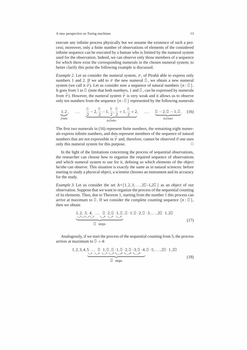
Example 2.Let us consider the numeral system,P , of Piraha able to express onlynumbers 1 and 2. If we add toP the new numeral①, we obtain a new numeralsystem (we call itP ). Let us consider now a sequence of natural numbers{n : ①}.It goes from 1 to① (note that both numbers, 1 and①, can be expressed by numeralsfrom P ). However, the numeral systemP is very weak and it allows us to observeonly ten numbers from the sequence{n : ①} represented by the following numerals

1,2︸︷︷︸f inite

, . . .①

2−2,

①

2−1,

①

2,

①

2+1,

①

2+2

︸︷︷︸in f inite

, . . . ①−2,①−1,①︸︷︷︸in f inite

. (16)

The first two numerals in (16) represent finite numbers, the remaining eight numer-als express infinite numbers, and dots represent members of the sequence of naturalnumbers that are not expressible inP and, therefore, cannot be observed if one usesonly this numeral system for this purpose. 2

In the light of the limitations concerning the process of sequential observations,the researcher can choose how to organize the required sequence of observationsand which numeral system to use for it, defining so which elements of the objecthe/she can observe. This situation is exactly the same as in natural sciences: beforestarting to study a physical object, a scientist chooses an instrument and its accuracyfor the study.

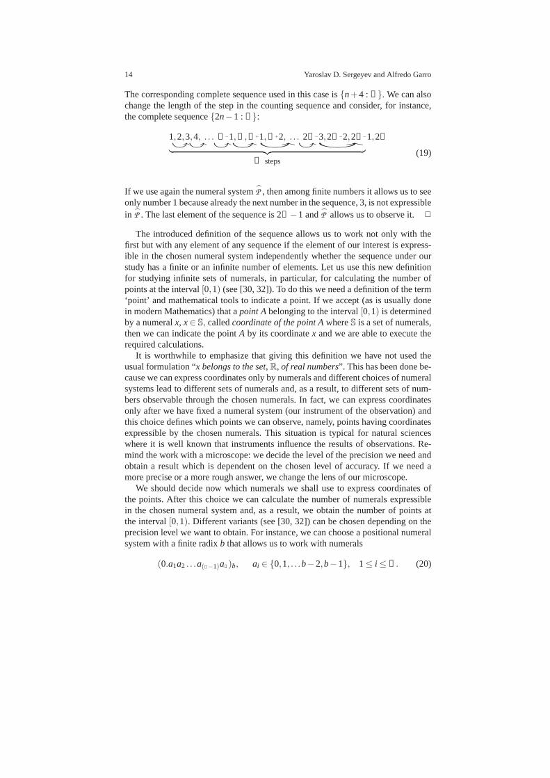
Example 3.Let us consider the set A={1,2,3, . . . ,2①-1,2①} as an object of ourobservation. Suppose that we want to organize the process ofthe sequential countingof its elements. Then, due to Theorem 1, starting from the number 1 this process canarrive at maximum to①. If we consider the complete counting sequence{n : ①},then we obtain

1,2, 3, 4, . . . ①−2,①−1,①,①+1,①+2,①+3, . . . ,2①−1,2①xxxx xx x

︸︷︷︸① steps

(17)

Analogously, if we start the process of the sequential counting from 5, the processarrives at maximum to①+4:

1,2,3,4,5 . . . ①−1,①,①+1,①+2,①+3,①+4,①+5, . . . ,2①−1,2①x xxx xxx


(18)


The corresponding complete sequence used in this case is{n+4 : ①}. We can alsochange the length of the step in the counting sequence and consider, for instance,the complete sequence{2n−1 : ①}:

1,2,3,4, . . . ①−1,①,①+1,①+2, . . . 2①−3,2①−2,2①−1,2①xx x x xx x


(19)

If we use again the numeral systemP , then among finite numbers it allows us to seeonly number 1 because already the next number in the sequence, 3, is not expressiblein P . The last element of the sequence is 2①−1 andP allows us to observe it. 2

The introduced definition of the sequence allows us to work not only with thefirst but with any element of any sequence if the element of ourinterest is express-ible in the chosen numeral system independently whether thesequence under ourstudy has a finite or an infinite number of elements. Let us use this new definitionfor studying infinite sets of numerals, in particular, for calculating the number ofpoints at the interval[0,1) (see [30, 32]). To do this we need a definition of the term‘point’ and mathematical tools to indicate a point. If we accept (as is usually donein modern Mathematics) that apoint Abelonging to the interval[0,1) is determinedby a numeralx, x∈ S, calledcoordinate of the point AwhereS is a set of numerals,then we can indicate the pointA by its coordinatex and we are able to execute therequired calculations.

It is worthwhile to emphasize that giving this definition we have not used theusual formulation “x belongs to the set,R, of real numbers”. This has been done be-cause we can express coordinates only by numerals and different choices of numeralsystems lead to different sets of numerals and, as a result, to different sets of num-bers observable through the chosen numerals. In fact, we canexpress coordinatesonly after we have fixed a numeral system (our instrument of the observation) andthis choice defines which points we can observe, namely, points having coordinatesexpressible by the chosen numerals. This situation is typical for natural scienceswhere it is well known that instruments influence the resultsof observations. Re-mind the work with a microscope: we decide the level of the precision we need andobtain a result which is dependent on the chosen level of accuracy. If we need amore precise or a more rough answer, we change the lens of our microscope.

We should decide now which numerals we shall use to express coordinates ofthe points. After this choice we can calculate the number of numerals expressiblein the chosen numeral system and, as a result, we obtain the number of points atthe interval[0,1). Different variants (see [30, 32]) can be chosen depending on theprecision level we want to obtain. For instance, we can choose a positional numeralsystem with a finite radixb that allows us to work with numerals

(0.a1a2 . . .a(①−1)a①)b, ai ∈ {0,1, . . .b−2,b−1}, 1≤ i ≤ ①. (20)


Then, the number of numerals (20) gives us the number of points within the inter-val [0,1) that can be expressed by these numerals. Note that a number using thepositional numeral system (20) cannot have more than grossone digits (contrarilyto sets discussed in Example 3) because a numeral havingg> ① digits would notbe observable in a sequence. In this case (g> ①) such a record becomes useless insequential computations because it does not allow one to identify numbers entirelysinceg−① numerals remain non observed.

Theorem 2. If coordinates of points x∈ [0,1) are expressed by numerals (20), thenthe number of the points x over[0,1) is equal to b①.

Proof.In the numerals (20) there is a sequence of digits,a1a2 . . .a(①−1)a①, used toexpress the fractional part of the number. Due to the definition of the sequence andTheorem 1, any infinite sequence can have at maximum① elements. As a result,there is① positions on the right of the dot that can be filled in by one of theb digitsfrom the alphabet{0,1, . . . ,b− 1} that leads tob① possible combinations. Hence,the positional numeral system using the numerals of the form(20) can expressb①

numbers. 2

Corollary 1. The number of numerals

(a1a2a3 . . .a①−2a①−1a①)b, ai ∈ {0,1, . . .b−2,b−1}, 1≤ i ≤ ①, (21)

expressing integers in the positional system with a finite radix b in the alphabet{0,1, . . .b−2,b−1} is equal to b①.

Proof.The proof is a straightforward consequence of Theorem 2 and is so omit-ted. 2

Corollary 2. If coordinates of points x∈ (0,1) are expressed by numerals (20), thenthe number of the points x over(0,1) is equal to b① −1.

Proof.The proof follows immediately from Theorem 2. 2

Note that Corollary 2 shows that it becomes possible now to observe and to reg-ister the difference of the number of elements of two infinitesets (the interval[0,1)and the interval(0,1), respectively) even when only one element (the point 0, ex-pressed by the numeral 0.00. . .0 with ① zero digits after the decimal point) has beenexcluded from the first set in order to obtain the second one.

4 Observing Turing machines through the lens of the GrossoneMethodology

In this Section the different types of Turing machines introduced in Section 2 areanalyzed and observed by using as instruments of observation the Grossone lan-guage and methodology presented in Section 3 . In particular, after introducing a


distiction between physical and ideal Turing machine (see Section 4.1), some re-sults for Single-tape and Multi-tape Turing machines are summarized (see Sections4.2 and 4.3 respectively), then a discussion about the equivalence between Singleand Multi-tape Turing machine is reported in Section 4.4. Finally, a comparison be-tween deterministic and non-deterministic Turing machines through the lens of theGrossone methodology is presented in Section 4.5.

4.1 Physical and Ideal Turing machines

Before starting observing Turing machines by using the Grossone methodology, itis useful to recall the main results showed in the previous Section: (i) a (complete)sequence can have maximum① elements; (ii) the elements which we are able toobserve in this sequence depend on the adopted numeral system. Moreover, a distic-tion between physical and ideal Turing machines should be introduced. Specifically,the machines defined in Section 2 (e.g. the Single-Tape Turing machine of Section2.1) are called ideal Turing machine,T I . Howerver, in order to study the limita-tions of practical automatic computations, we also consider machines,T P , that canbe constructed physically. They are identical toT I but are able to work only a finitetime and can produce only finite outputs. In this Section, both kinds of machinesare analyzed from the point of view of their outputs, called by Turing ‘computablenumbers’ or ‘computable,sequences’, and from the point of view of computationsthat the machines can execute .

Let us consider first a physical machineT P and discuss about the number ofcomputational steps it can execute and how the obtained results then can be inter-preted by a human observer (e.g. the researcher) . We supposethat its output iswritten on the tape using an alphabetΣ containingb symbols{0,1, . . .b−2,b−1}whereb is a finite number (Turing usesb = 10).Thus, the output consists of a se-quence of digits that can be viewed as a number in a positionalsystemB with theradix b. By definition,T P should stop after a finite number of iterations. The mag-nitude of this value depends on the physical construction ofthe machine, the waythe notion ‘iteration’ has been defined, etc., but in any casethis number is finite.A physical machineT P stops in two cases: (i) it has finished the execution of itsprogram and stops; (ii) it stops because its breakage. In both cases the output se-quence

(a1a2a3 . . .ak−1,ak)b, ai ∈ {0,1, . . .b−2,b−1}, 1≤ i ≤ k,

of T P has a finite lengthk.If the maximal length of the output sequence that can be computed byT P is

equal to a finite numberKT P , then it followsk ≤ KT P . This means that there existproblems that cannot be solved byT P if the length of the output outnumbersKT P .If a physical machineT P has stopped after it has printedKT P symbols, then it is


not clear whether the obtained output is a solution or just a result of the depletion ofits computational resources.In particular, with respect to the halting problem it follows that all algorithms stoponT P .

In order to be able to read and to understand the output, the researcher (the user)should know a positional numeral systemU with an alphabet{0,1, . . .u−2,u−1}whereu ≥ b. Otherwise, the output cannot be decoded by the user. Moreover, theresearcher must be able to observe a number of symbols at least equal to the maximallength of the output sequence that can be computed by machine(i.e.,KU ≥ KT P ).

If the situationKU < KT P holds, then this means that the user is not able to inter-pret the obtained result. Thus, the numberK∗ = min{KU ,KT P } defines the lengthof the outputs that can be computed and interpreted by the user.As a consequence, algorithms producing outputs having morethanK∗ positions be-come less interesting from the practical point of view.

After having introduced the distinction between physical and ideal Turing ma-chines, let us analyze and observe them through the lens of the Grossone Method-ology. Specifically, the results obtained and discussed in [42] for deterministic andnon-deterministic Single-tape Turing machines are summarized in Section 4.2 and4.4 respectively; whereas, Section 4.3 reports additionalresults for Multi-tape Tur-ing machines (see [43]).

4.2 Observing Single-Tape Turing machines

As stated in Section 4.1, single-tape ideal Turing machinesM I (see Section 2.1)can produce outputs with an infinite number of symbolsk. However, in order to beobservable in a sequence, an output should havek ≤ ① (see Section 3). Startingfrom these considerations the following theorem can be introduced.

Theorem 3. Let M be the number of all possible complete computable sequencesthat can be produced by ideal single-tape Turing machines using outputs being nu-merals in the positional numeral systemB . Then it follows M≤ b①.

Proof.This result follows from the definitions of the complete sequence and theform of numerals

(a−1a−2 . . .a−(①−1)a−①)b, a−i ∈ {0,1, . . .b−2,b−1}, 1≤ i ≤ ①,

that are used in the positional numeral systemB . 2

Corollary 3. Let us consider an ideal Turing machineM I1 working with the alpha-

bet{0,1,2} and computing the following complete computable sequence


0,1,2,0,1,2,0,1,2, . . . 0,1,2,0,1,2︸︷︷︸① positions

. (22)

Then ideal Turing machines working with the output alphabet{0,1} cannot produceobservable in a sequence outputs computing (22).

Since the numeral 2 does not belong to the alphabet{0,1} it should be coded bymore than one symbol. One of codifications using the minimal number of symbolsin the alphabet{0,1} necessary tocode numbers 0,1,2 is {00,01,10}. Then theoutput corresponding to (22) and computed in this codification should be

00,01,10,00,01,10,00,01,10, . . . 00,01,10,00,01,10. (23)

Since the output (22) contains grossone positions, the output (23) should contain2① positions. However, in order to be observable in a sequence,(23) should nothave more than grossone positions. This fact completes the proof. 2

The mathematical language used by Turing did not allow one todistinguish thesetwo machines. Now we are able to distinguish a machine from another also whenwe consider infinite sequences. Turing’s results and the newones do not contradicteach other. Both languages observe and describe the same object (computable se-quences) but with different accuracies.

It is not possible to describe a Turing machine (the object ofthe study) withoutthe usage of a numeral system (the instrument of the study). As a result, it becomesnot possible to speak about an absolute number of all possible Turing machinesT I .It is always necessary to speak about the number of all possible Turing machinesT I expressible in a fixed numeral system (or in a group of them).

Theorem 4. The maximal number of complete computable sequences produced byideal Turing machines that can be enumerated in a sequence isequal to①.

We have established that the number of complete computable sequences that canbe computed using a fixed radixb is less or equalb①. However, we do not knowhow many of them can be results of computations of a Turing machine. Turing es-tablishes that their number is enumerable. In order to obtain this result, he used themathematical language developed by Cantor and this language did not allow himto distinguish sets having different infinite numbers of elements. The introductionof grossone gives a possibility to execute a more precise analysis and to distinguishwithin enumerable sets infinite sets having different numbers of elements. For in-

stance, the set of even numbers has①2 elements and the set of integer numbers has

2①+1 elements. If the number of complete computable sequences,MT I , is largerthan①, then there can be differen sequential processes that enumerate different se-quences of complete computable sequences. In any case, eachof these enumeratingsequential processes cannot contain more than grossone members.


4.3 Observing Multi-tape Turing machines

Before starting to analyze the computations performed by anideal k-tapes Turing

machine (withk ≥ 2) M IK =

⟨Q,Γ, b,Σ,q0,F,δ(k)

⟩(see (1), see Section 2.2), it is

worth to make some considerations about the process of observation itself in thelight of the Grossone methodology. As discussed above, if wewant to observe theprocess of computation performed by a Turing machine while it executes an al-gorithm, then we have to execute observations of the machinein a sequence ofmoments. In fact, it is not possible to organize a continuousobservation of the ma-chine. Any instrument used for an observation has its accuracy and there always bea minimal period of time related to this instrument allowingone to distinguish twodifferent moments of time and, as a consequence, to observe (and to register) thestates of the object in these two moments. In the period of time passing betweenthese two moments the object remains unobservable.

Since our observations are made in a sequence, the process ofobservations canhave at maximum① elements. This means that inside a computational process itispossible to fix more than grossone steps (defined in a way) but it is not possible tocount them one by one in a sequence containing more than grossone elements. Forinstance, in a time interval[0,1), up tob① numerals of the type (20) can be usedto identify moments of time but not more than grossone of themcan be observedin a sequence. Moreover, it is important to stress that any process itself, consideredindependently on the researcher, is not subdivided in iterations, intermediate results,moments of observations, etc. The structure of the languagewe use to describethe process imposes what we can say about the process (see [42] for a detaileddiscussion).

On the basis of the considerations made above, we should choose the accuracy(granularity) of the process of the observation of a Turing machine; for instance wecan choose a single operation of the machine such as reading asymbol from thetape, or moving the tape, etc. However, in order to be close asmuch as possible tothe traditional results, we consider an application of the transition function of themachine as our observation granularity (see Section 2).

Moreover, concerning the output of the machine, we considerthe symbols writtenon all the k tapes of the machine by using, on each tapei, with 1 ≤ i ≤ k, thealphabetΣi of the tape, containingbi symbols, plus the blank symbol (b). Due tothe definition of complete sequence (see Section 3) on each tape at least① symbolscan be produced and observed. This means that on a tapei, after the last symbolsbelonging to the tape alphabetΣi , if the sequence is not complete (i.e., if it hasless than① symbols) we can consider a number of blank symbols (b) necessaryto complete the sequence. We say that we are considering acomplete outputof ak-tapes Turing machine when on each tape of the machine we consider a completesequence of symbols belonging toΣi ∪{b}.

Theorem 5. Let M IK =


⟩be an ideal k-tapes, k≥ 2, Turing

machine. Then, a complete output of the machine will resultsin k① symbols.


Proof.Due to the definition of the complete sequence, on each tape atmaximum① symbols can be produced and observed and thus by consideringa complete se-quence on each of the k tapes of the machine the complete output of the machinewill result in k① symbols. 2

Having proved that a complete output that can be produced by ak-tapes Turingmachine results ink① symbols, it is interesting to investigate what part of the com-plete output produced by the machine can be observed in a sequence taking intoaccount that it is not possible to observe in a sequence more than① symbols (seeSection 3). As examples, we can decide to make in a sequence one of the following

observations: (i)① symbols on one among thek-tapes of the machine, (ii)①k sym-

bols on each of thek-tapes of the machine; (iii)①2 symbols on 2 among thek-tapesof the machine, an so on.

Theorem 6. Let M IK =


⟩be an ideal k-tapes, k≥ 2, Turing

machine. Let M be the number of all possible complete outputsthat can be producedbyM I

K . Then it follows M= ∏ki=1 (bi +1)①.

Proof.Due to the definition of the complete sequence, on each tapei, with 1≤ i ≤k, at maximum① symbols can be produced and observed by using thebi symbolsof the alphabetΣi of the tape plus the blank symbol (b); as a consequence, thenumber of all the possible complete sequences that can be produced and observedon a tapei is (bi +1)①. A complete output of the machine is obtained by consideringa complete sequence on each of the thek-tapes of the machine, thus by consideringall the possible complete sequences that can be produced andobserved on each ofthe k tapes of the machine, the numberM of all the possible complete outputs willresults in∏k

i=1 (bi +1)①. 2

As the numberM = ∏ki=1 (bi +1)① of complete outputs that can be produced

by M K is larger than grossone, then there can be different sequential enumeratingprocesses that enumerate complete outputs in different ways, in any case, each ofthese enumerating sequential processes cannot contain more than grossone members(see Section 3).

4.4 Comparing different Multi-tape machines and Multi andSingle-tape machines

In the classical framework idealk-tape Turing machines have the same computa-tional power of Single-tape Turing machines and given a Multi-tape Turing ma-chineM I

K it is always possible to define a Single-tape Turing machine which is ableto fully simulate its behavior and therefore to completely execute its computations.As showed for Single-tape Turing machine (see [42]), the Grossone methodologyallows us to give a more accurate definition of the equivalence among different ma-chines as it provides the possibility not only to separate different classes of infinitesets with respect to their cardinalities but also to measurethe number of elements


of some of them. With reference to Multi-tape Turing machines, the Single-tapeTuring machines adopted for their simulation use a particular kind of tape which isdivided into tracks (multi-track tape). In this way, if the tape hasm tracks, the headis able to access (for reading and/or writing) all them characters on the tracks dur-ing a single operation. This tape organization leads to a straightforward definition ofthe behavior of a Single-tape Turing machine able to completely execute the com-putations of a given Multi-tape Turing machine (see Section2.2). However, the sodefined Single-tape Turing machineM I , to simulatet computational steps ofM I

K ,needs to executeO(t2) transitions (t2+ t in the worst case) and to use an alphabetwith 2k(|Σ1|+1)∏k

i=2(|Σi |+2) symbols (again see Section 2.2). By exploiting theGrossone methodology is is possibile to obtain the following result that has a higheraccuracy with respect to that provided by the traditional framework.

Theorem 7. Let us considerM IK =


⟩,a k-tapes, k≥ 2, Turing

machine, whereΣ =⋃k

i=1 Σi is given by the union of the symbols in the k tape al-phabetsΣ1, . . . ,Σk andΓ = Σ∪{b}. If this machine performs t computational stepssuch that

t 612(√

4①+1−1), (24)

then there existsM I1 = {Q′,Γ′, b,Σ′,q′0,F

′,δ′}, an equivalent Single-tape Turingmachine with|Γ′| = 2k(|Σ1|+1)∏k

i=2(|Σi |+2), which is able to simulateM IK and

can be observed in a sequence.

Proof. Let us recall that the definition ofM I1 requires for a Single-tape to be

divided into 2k tracks;k tracks for storing the characters in thek tapes ofM IK and

k tracks for signing through the marker↓ the positions of thek heads on thektapes ofM I

k (see Section 2.2). The transition functionδ(k) of the k-tapes machineis given byδ(k)(q1,ai1, . . . ,ai k) = (q j ,a j 1, . . . ,a j k,zj 1, . . . ,zj k), with zj 1, . . . ,zj k ∈{R,L,N}; as a consequence the corresponding transition functionδ′ of the Single-tape machine, for each transition specified byδ(k) must individuate the current stateand the position of the marker for each track and then write onthe tracks the requiredsymbols, move the markers and go in another internal state. For each computationalstep ofM I

K , M I1 must execute a sequence of steps for covering the portion of tapes

between the two most distant markers. As in each computational step a marker canmove at most of one cell and then two markers can move away eachother at mostof two cells, aftert steps ofM I

K the markers can be at most 2t cells distant, thusif M I

K executest steps,M I1 executes at most: 2∑t

i=1 i = t2+ t steps. In order to beobservable in a sequence the numbert2+ t of steps, performed byM I

1 to simulatetsteps ofM I

K , must be less than or equal to①. Namely, it should bet2+ t 6①. Thefact that this inequality is satisfied fort 6 1

2(√

4①+1−1) completes the proof.2


4.5 Comparing deterministic and non-deterministic Turingmachines

Let us discuss the traditional and new results regarding thecomputational power ofdeterministic and non-deterministic Turing machines.

Classical results show an exponential growth of the time required for reachinga final configuration by the deterministic Turing machineMD with respect to thetime required by the non-deterministic Turing machineMN, assuming that the timerequired for both machines for a single step is the same. However, in the classictheory on Turing machines it is not known if there is a more efficient simulation ofMN. In other words, it is an important and open problem of Computer Science theoryto demonstrate that it is not possible to simulate a non-deterministic Turing machineby a deterministic Turing machine with a sub-exponential numbers of steps.

Let us now return to the new mathematical language. Since themain interest tonon-deterministic Turing machines (5) is related to their theoretical properties, here-inafter we start by a comparison of ideal deterministic Turing machines,T I , withideal non-deterministic Turing machinesT I N . Physical machinesT P andT P N areconsidered at the end of this section. By taking into accountthe results of Section4.4, the proposed approach can be applied both to single and multi-tape machines,however, single-tape machines are considered in the following.

Due to the analysis made in Section 4.3, we should choose the accuracy (gran-ularity) of processes of observation of both machines,T I andT I N . In order to beclose as much as possible to the traditional results, we consider again an applica-tion of the transition function of the machine as our observation granularity. Withrespect toT I N this means that the nodes of the computational tree are observed.With respect toT I we consider sequences of such nodes. For both cases the ini-tial configuration is not observed, i.e., we start our observations from level 1 of thecomputational tree.

This choice of the observation granularity is particularlyattractive due to its ac-cordance with the traditional definitions of Turing machines (see definitions (1) and(5)). A more fine granularity of observations allowing us to follow internal oper-ations of the machines can be also chosen but is not so convenient. In fact, suchan accuracy would mix internal operations of the machines with operations of thealgorithm that is executed. A coarser granularity could be considered, as well. Forinstance, we could define as a computational step two consecutive applications ofthe transition function of the machine. However, in this case we do not observe allthe nodes of the computational tree. As a consequence, we could miss some resultsof the computation as the machine could reach a final configuration before complet-ing an observed computational step and we are not able to observe when and onwhich configuration the machine stopped. Then, fixed the chosen level of granular-ity the following result holds immediately.

Theorem 8. (i) With the chosen level of granularity no more than① computationalsteps of the machineT I can be observed in a sequence. (ii) In order to give possi-bility to observe at least one computational path of the computational tree ofT I N


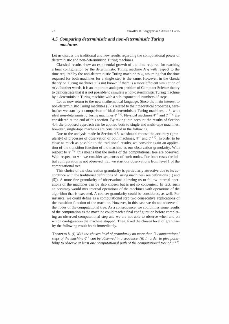
Fig. 2 The maximum number of computational steps of the machineT I that can be observed in asequence

from the level 1 to the level k, the depth, k≥ 1, of the computational tree cannot belarger than grossone, i.e., k≤ ①.

Proof.Both results follow from the analysis made in Section 3.1 andTheorem 1.2

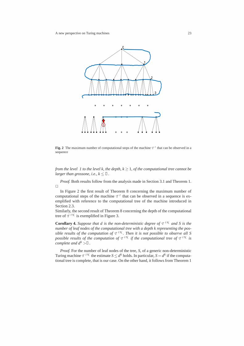
In Figure 2 the first result of Theorem 8 concerning the maximum number ofcomputational steps of the machineT I that can be observed in a sequence is ex-emplified with reference to the computational tree of the machine introduced inSection 2.3.Similarly, the second result of Theorem 8 concerning the depth of the computationaltree ofT I N is exemplified in Figure 3.

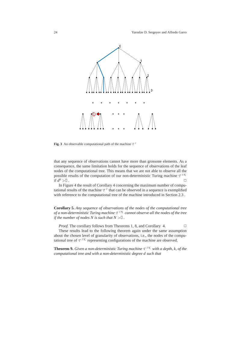
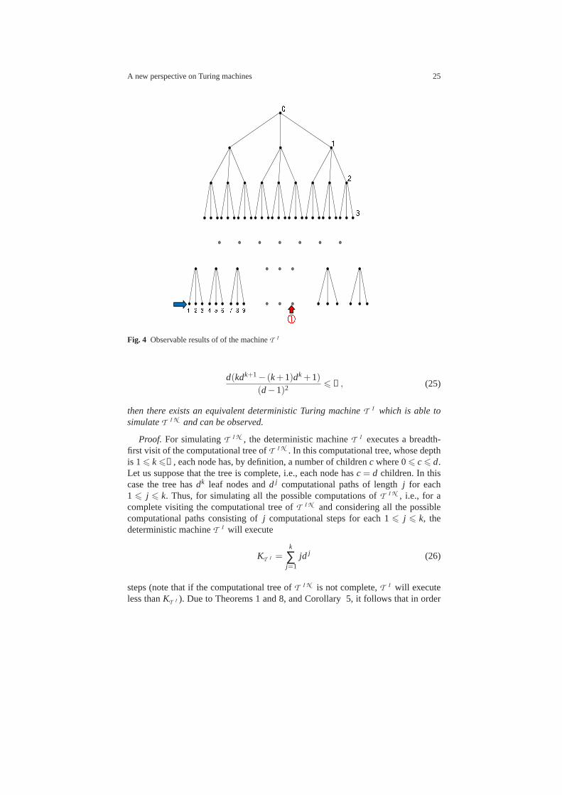
Corollary 4. Suppose that d is the non-deterministic degree ofT I N and S is thenumber of leaf nodes of the computational tree with a depth k representing the pos-sible results of the computation ofT I N . Then it is not possible to observe all Spossible results of the computation ofT I N if the computational tree ofT I N iscomplete and dk >①.

Proof.For the number of leaf nodes of the tree,S, of a generic non-deterministicTuring machineT I N the estimateS≤ dk holds. In particular,S= dk if the computa-tional tree is complete, that is our case. On the other hand, it follows from Theorem 1


Fig. 3 An observable computational path of the machineT I

that any sequence of observations cannot have more than grossone elements. As aconsequence, the same limitation holds for the sequence of observations of the leafnodes of the computational tree. This means that we are not able to observe all thepossible results of the computation of our non-deterministic Turing machineT I N

if dk >①. 2

In Figure 4 the result of Corollary 4 concerning the maximum number of compu-tational results of the machineT I that can be observed in a sequence is exemplifiedwith reference to the computational tree of the machine introduced in Section 2.3 .

Corollary 5. Any sequence of observations of the nodes of the computational treeof a non-deterministic Turing machineT I N cannot observe all the nodes of the treeif the number of nodes N is such that N>①.

Proof.The corollary follows from Theorems 1, 8, and Corollary 4. 2

These results lead to the following theorem again under the same assumptionabout the chosen level of granularity of observations, i.e., the nodes of the compu-tational tree ofT I N representing configurations of the machine are observed.

Theorem 9. Given a non-deterministic Turing machineT I N with a depth, k, of thecomputational tree and with a non-deterministic degree d such that


Fig. 4 Observable results of of the machineT I

d(kdk+1− (k+1)dk+1)(d−1)2 6 ①, (25)

then there exists an equivalent deterministic Turing machine T I which is able tosimulateT I N and can be observed.

Proof. For simulatingT I N , the deterministic machineT I executes a breadth-first visit of the computational tree ofT I N . In this computational tree, whose depthis 16 k6①, each node has, by definition, a number of childrenc where 06 c6 d.Let us suppose that the tree is complete, i.e., each node hasc= d children. In thiscase the tree hasdk leaf nodes andd j computational paths of lengthj for each1 6 j 6 k. Thus, for simulating all the possible computations ofT I N , i.e., for acomplete visiting the computational tree ofT I N and considering all the possiblecomputational paths consisting ofj computational steps for each 16 j 6 k, thedeterministic machineT I will execute

KT I =k

∑j=1

jd j (26)

steps (note that if the computational tree ofT I N is not complete,T I will executeless thanKT I ). Due to Theorems 1 and 8, and Corollary 5, it follows that in order


to prove the theorem it is sufficient to show that under conditions of the theorem itfollows that

KT I 6 ①. (27)

To do this let us use the well known formula

k

∑j=0

d j =dk+1−1

d−1, (28)

and derive both parts of (28) with respect tod. As the result we obtain

k

∑j=1

jd j−1 =kdk+1− (k+1)dk+1

(d−1)2 . (29)

Notice now that by using (26) it becomes possible to represent the numberKT I as

KT I =k

∑j=1

jd j = dk

∑j=1

jd j−1.

This representation together with (29) allow us to write

KT I =d(kdk+1− (k+1)dk+1)

(d−1)2 (30)

Due to assumption (25), it follows that (27) holds. This factconcludes the proof ofthe theorem. 2

Corollary 6. Suppose that the length of the input sequence of symbols of a non-deterministic Turing machineT I N is equal to a number n andT I N has a completecomputational tree with the depth k such that k= nl , i.e., polynomially depends onthe length n. Then, if the values d,n, and l satisfy the following condition

d(nl dnl+1− (nl +1)dnl+1)

(d−1)2 6 ①, (31)

then: (i) there exists a deterministic Turing machineT I that can be observed andable to simulateT I N ; (ii) the number, KT I , of computational steps required to adeterministic Turing machineT I to simulateT I N for reaching a final configurationexponentially depends on n.

Proof.The first assertion follows immediately from theorem 9. Let us prove thesecond assertion. Since the computational tree ofT I N is complete and has the depthk, the corresponding deterministic Turing machineT I for simulatingT I N will ex-ecuteKT I steps whereKT I is from (27). Since condition (31) is satisfied forT I N ,we can substitutek= nl in (30). As the result of this substitution and (31) we obtainthat


KT I =d(nl dnl+1− (nl +1)dnl

+1)(d−1)2 6 ①, (32)

i.e., the number of computational steps required to the deterministic Turing machineT I to simulate the non-deterministic Turing machineT I N for reaching a final con-figuration isKT I 6 ① and this number exponentially depends on the length of thesequence of symbols provided as input toT I N . 2

Results described in this section show that the introduction of the new mathemat-ical language including grossone allows us to perform a moresubtle analysis withrespect to traditional languages and to introduce in the process of this analysis thefigure of the researcher using this language (more precisely, to emphasize the pres-ence of the researcher in the process of the description of automatic computations).These results show that there exist limitations for simulating non-deterministic Tur-ing machines by deterministic ones. These limitations can be viewed now thanks tothe possibility (given because of the introduction of the new numeral①) to observefinal points of sequential processes for both cases of finite and infinite processes.

Theorems 8, 9, and their corollaries show that the discovered limitations andrelations between deterministic and non-deterministic Turing machines have stronglinks with our mathematical abilities to describe automatic computations and to con-struct models for such descriptions. Again, as it was in the previous cases studiedin this chapter, there is no contradiction with the traditional results because bothapproaches give results that are correct with respect to thelanguages used for therespective descriptions of automatic computations.

We conclude this section by the note that analogous results can be obtained forphysical machinesT P andT P N , as well. In the case of ideal machines, the pos-sibility of observations was limited by the mathematical languages. In the case ofphysical machines they are limited also by technical factors (we remind again theanalogy: the possibilities of observations of physicists are limited by their instru-ments). In any given moment of time the maximal number of iterations,Kmax, thatcan be executed by physical Turing machines can be determined. It depends on thespeed of the fastest machineT P available at the current level of development ofthe humanity, on the capacity of its memory, on the time available for simulatinga non-deterministic machine, on the numeral systems known to human beings, etc.Together with the development of technology this number will increase but it willremain finite and fixed in any given moment of time. As a result,theorems presentedin this section can be re-written forT P andT P N by substituting grossone withKmax

in them.

5 Concluding Remarks

Since the beginning of the last century, the fundamental nature of the concept ofautomatic computationsattracted a great attention of mathematicians and computerscientists (see [4, 14, 15, 16, 23, 24, 27, 44]). The first studies had as their ref-


erence context the David Hilbert programme, and as their reference language thatintroduced by Georg Cantor [3]. These approaches lead to different mathematicalmodels of computing machines (see [1, 6, 9]) that, surprisingly, were discoveredto be equivalent (e.g., anything computable in theλ-calculus is computable by aTuring machine). Moreover, these results, and expecially those obtained by AlonzoChurch, Alan Turing [4, 10, 44] and Kurt Godel, gave fundamental contributions todemonstrate that David Hilbert programme, which was based on the idea that all ofthe Mathematics could be precisely axiomatized, cannot be realized.

In spite of this fact, the idea of finding an adequate set of axioms for one oranother field of Mathematics continues to be among the most attractive goals forcontemporary mathematicians. Usually, when it is necessary to define a concept oran object, logicians try to introduce a number of axioms describing the object inthe absolutely best way. However, it is not clear how to reachthis absoluteness;indeed, when we describe a mathematical object or a concept we are limited bythe expressive capacity of the language we use to make this description. A richerlanguage allows us to say more about the object and a weaker language – less.Thus, the continuous development of the mathematical (and not only mathematical)languages leads to a continuous necessity of a transcription and specification ofaxiomatic systems. Second, there is no guarantee that the chosen axiomatic systemdefines ‘sufficiently well’ the required concept and a continuous comparison withpractice is required in order to check the goodness of the accepted set of axioms.However, there cannot be again any guarantee that the new version will be the lastand definitive one. Finally, the third limitation already mentioned above has beendiscovered by Godel in his two famous incompleteness theorems (see [10]).

Starting from these considerations, in the chapter, Singleand Multi-tape Turingmachines have been described and observed through the lens of the Grossone lan-guage and methodology . This new language, differently fromthe traditional one,makes it possible to distinguish among infinite sequences ofdifferent length so en-abling a more accurate description of Single and Multi-tapeTuring machines. Thepossibility to express the length of an infinite sequence explicitly gives the pos-sibility to establish more accurate results regarding the equivalence of machines incomparison with the observations that can be done by using the traditional language.

It is worth noting that the traditional results and those presented in the chapterdo not contradict one another. They are just written by usingdifferent mathematicallanguages having different accuracies. Both mathematicallanguages observe anddescribe the same objects – Turing machines – but with different accuracies. As aresult, both traditional and new results are correct with respect to the mathematicallanguages used to express them and correspond to different accuracies of the obser-vation. This fact is one of the manifestations of the relativity of mathematical resultsformulated by using different mathematical languages in the same way as the usageof a stronger lens in a microscope gives a possibility to distinguish more objectswithin an object that seems to be unique when viewed by a weaker lens.

Specifically, the Grossone language has allowed us to give the definition ofcom-plete outputof a Turing machine, to establish when and how the output of a ma-chine can be observed, and to establish a more accurate relationship between Multi-


tape and Single-tape Turing machines as well as between deterministic and non-deterministic ones. Future research efforts will be gearedto apply the Grossonelanguage and methodology to the description and observation of new and emergingcomputational paradigms.

References

1. G. Ausiello, F. D’Amore, and G. Gambosi.Linguaggi, modelli, complessita. Franco AngeliEditore, Milan, 2 edition, 2006.

2. V. Benci and M. Di Nasso. Numerosities of labeled sets: a new way ofcounting.Advances inMathematics, 173:50–67, 2003.

3. G. Cantor.Contributions to the founding of the theory of transfinite numbers. Dover Publica-tions, New York, 1955.

4. A. Church. An unsolvable problem of elementary number theory. American Journal of Math-ematics, 58:345–363, 1936.

5. J.H. Conway and R.K. Guy.The Book of Numbers. Springer-Verlag, New York, 1996.6. S. Barry Cooper.Computability Theory. Chapman Hall/CRC, 2003.7. S. De Cosmis and R. De Leone. The use of Grossone in mathematical programming and

operations research.Applied Mathematics and Computation, 218(16):8029–8038, 2012.8. L. D’Alotto. Cellular automata using infinite computations.Applied Mathematics and Com-

putation, 218(16):8077–8082, 2012.9. M. Davis.Computability& Unsolvability. Dover Publications, New York, 1985.

10. K. Godel. Uber formal unentscheidbare Satze der Principia Mathematica und verwandterSysteme.Monatshefte fur Mathematik und Physik, 38:173–198, 1931.

11. P. Gordon. Numerical cognition without words: Evidence from Amazonia.Science, 306(15October):496–499, 2004.

12. J. Hopcroft and J. Ullman.Introduction to Automata Theory, Languages and Computation.Addison-Wesley, Reading Mass., 1st edition, 1979.

13. D.I. Iudin, Ya.D. Sergeyev, and M. Hayakawa. Interpretation of percolation in terms of infinitycomputations.Applied Mathematics and Computation, 218(16):8099–8111, 2012.

14. S.C. Kleene.Introduction to metamathematics. D. Van Nostrand, New York, 1952.15. A.N. Kolmogorov. On the concept of algorithm.Uspekhi Mat. Nauk, 8(4):175–176, 1953.16. A.N. Kolmogorov and V.A. Uspensky. On the definition of algorithm. Uspekhi Mat. Nauk,

13(4):3–28, 1958.17. G.W. Leibniz and J.M. Child.The Early Mathematical Manuscripts of Leibniz. Dover Publi-

cations, New York, 2005.18. T. Levi-Civita. Sui numeri transfiniti.Rend. Acc. Lincei, Series 5a, 113:7–91, 1898.19. G. Lolli. Metamathematical investigations on the theory ofGrossone.to appear in Applied

Mathematics and Computation.20. G. Lolli. Infinitesimals and infinites in the history of mathematics: A brief survey. Applied

Mathematics and Computation, 218(16):7979–7988, 2012.21. M. Margenstern. Using Grossone to count the number of elements of infinite sets and the con-

nection with bijections.p-Adic Numbers, Ultrametric Analysis and Applications, 3(3):196–204, 2011.

22. M. Margenstern. An application of Grossone to the study of a family of tilings of the hyper-bolic plane.Applied Mathematics and Computation, 218(16):8005–8018, 2012.

23. A.A. Markov Jr. and N.M. Nagorny.Theory of Algorithms. FAZIS, Moscow, second edition,1996.

24. J.P. Mayberry.The Foundations of Mathematics in the Theory of Sets. Cambridge UniversityPress, Cambridge, 2001.

25. I. Newton.Method of Fluxions. 1671.


26. P. Pica, C. Lemer, V. Izard, and S. Dehaene. Exact and approximate arithmetic in an amazonianindigene group.Science, 306(15 October):499–503, 2004.

27. E. Post. Finite combinatory processes – formulation 1.Journal of Symbolic Logic, 1:103–105,1936.

28. A. Robinson.Non-standard Analysis. Princeton Univ. Press, Princeton, 1996.29. E.E. Rosinger. Microscopes and telescopes for theoreticalphysics: How rich locally and large

globally is the geometric straight line?Prespacetime Journal, 2(4):601–624, 2011.30. Ya.D. Sergeyev.Arithmetic of Infinity. Edizioni Orizzonti Meridionali, CS, 2003.31. Ya.D. Sergeyev. Blinking fractals and their quantitative analysis using infinite and infinitesi-

mal numbers.Chaos, Solitons& Fractals, 33(1):50–75, 2007.32. Ya.D. Sergeyev. A new applied approach for executing computations with infinite and in-

finitesimal quantities.Informatica, 19(4):567–596, 2008.33. Ya.D. Sergeyev. Evaluating the exact infinitesimal valuesof area of Sierpinski’s carpet and

volume of Menger’s sponge.Chaos, Solitons& Fractals, 42(5):3042–3046, 2009.34. Ya.D. Sergeyev. Numerical computations and mathematical modelling with infinite and in-

finitesimal numbers.Journal of Applied Mathematics and Computing, 29:177–195, 2009.35. Ya.D. Sergeyev. Numerical point of view on Calculus for functions assuming finite, infinite,

and infinitesimal values over finite, infinite, and infinitesimal domains. Nonlinear AnalysisSeries A: Theory, Methods& Applications, 71(12):e1688–e1707, 2009.

36. Ya.D. Sergeyev. Counting systems and the First Hilbert problem. Nonlinear Analysis SeriesA: Theory, Methods& Applications, 72(3-4):1701–1708, 2010.

37. Ya.D. Sergeyev. Lagrange Lecture: Methodology of numerical computations with infinitiesand infinitesimals.Rendiconti del Seminario Matematico dell’Universita e del Politecnico diTorino, 68(2):95–113, 2010.

38. Ya.D. Sergeyev. Higher order numerical differentiationon the infinity computer.OptimizationLetters, 5(4):575–585, 2011.

39. Ya.D. Sergeyev. On accuracy of mathematical languages usedto deal with the Riemann zetafunction and the Dirichlet eta function.p-Adic Numbers, Ultrametric Analysis and Applica-tions, 3(2):129–148, 2011.

40. Ya.D. Sergeyev. Using blinking fractals for mathematical modelling of processes of growth inbiological systems.Informatica, 22(4):559–576, 2011.

41. Ya.D. Sergeyev. Solving ordinary differential equations by working with infinitesimals nu-merically on the infinity computer.Applied Mathematics and Computation, 219(22):10668–10681, 2013.

42. Ya.D. Sergeyev and A. Garro. Observability of Turing machines: A refinement of the theoryof computation.Informatica, 21(3):425–454, 2010.

43. Ya.D. Sergeyev and A. Garro. Single-tape and Multi-tapeTuring Machines through the lensof the Grossone methodology.The Journal of Supercomputing, 65(2):645–663, 2013.

44. A.M. Turing. On computable numbers, with an application to the entscheidungsproblem.Proceedings of London Mathematical Society, series 2, 42:230–265, 1936-1937.

45. M.C. Vita, S. De Bartolo, C. Fallico, and M. Veltri. Usage of infinitesimals in the Menger’sSponge model of porosity.Applied Mathematics and Computation, 218(16):8187–8196, 2012.

46. J. Wallis.Arithmetica infinitorum. 1656.47. A.A. Zhigljavsky. Computing sums of conditionally convergent and divergent series using the

concept of Grossone.Applied Mathematics and Computation, 218(16):8064–8076, 2012.48. A. Zilinskas. On strong homogeneity of two global optimization algorithms based on sta-

tistical models of multimodal objective functions.Applied Mathematics and Computation,218(16):8131–8136, 2012.

The Grossone methodology perspective on Turing machines · 2015-01-29 · A new perspective on...

Documents

Transcript of The Grossone methodology perspective on Turing machines · 2015-01-29 · A new perspective on...