The Greek Letters - Florida International...
40
The Greek Letters Chapter 17 1
Transcript of The Greek Letters - Florida International...

The Greek LettersChapter 17
1
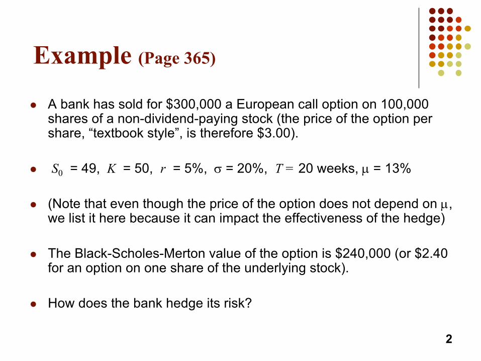
Example (Page 365)
l A bank has sold for $300,000 a European call option on 100,000 shares of a non-dividend-paying stock (the price of the option per share, “textbook style”, is therefore $3.00).
l S0 = 49, K = 50, r = 5%, s = 20%, T = 20 weeks, µ = 13%
l (Note that even though the price of the option does not depend on µ, we list it here because it can impact the effectiveness of the hedge)
l The Black-Scholes-Merton value of the option is $240,000 (or $2.40 for an option on one share of the underlying stock).
l How does the bank hedge its risk?
2

Naked & Covered Positions
l Naked position:
l One strategy is to simply do nothing: taking no action and remaining exposed to
the option risk.
l In this example, since the firm wrote/sold the call option, it hopes that the stock
remains below the strike price ($50) so that the option doesn’t get exercised by
the other party and the firm keeps the premium (price of the call it received
originally) in full.
l But if the stock rises to, say, $60, the firm loses (60-50)x100,000: a loss of
$1,000,000 is much more than the $300,000 received before.
l Covered position:
l The firm can instead buy 100,000 shares today in anticipation of having to deliver
them in the future if the stock rises.
l If the stock declines, however, the option is not exercised but the stock position is
hurt: if the stock goes down to $40, the loss is (49-40)x100,000 = $900,000.
3

Stop-Loss Strategy
l The stop-loss strategy is designed to ensure that the firm owns the stock if the option closes in-the-money and does not own the stock if the option closes out-of-the-money.
l The stop-loss strategy involves:l Buying 100,000 shares as soon as the stock
price reaches $50.l Selling 100,000 shares as soon as the stock
price falls below $50.4

Stop-Loss Strategy continued
5
However, repeated transactions (costly) and the fact that you will always buy at K+e and sell at K-e makes this strategy not a very viable one.

Delta (See Figure 17.2, page 369)
l Delta (D) is the rate of change of the option price with respect to the underlying
Optionprice
A
BSlope = D = 0.6
Stock price
6

Hedge
l Trader would be hedged with the position:l Short/wrote 1000 options (each on one share)l buy 600 shares
l Gain/loss on the option position is offset by loss/gain on stock position
l Delta changes as stock price changes and time passes.
l Hedge position must therefore be rebalanced often, an example of dynamic hedging.
7

Delta Hedging
l Delta hedging involves maintaining a delta neutral portfolio: a position with a delta of zero.
l The delta of a European call on a non-dividend-paying stock is N (d 1)
l The delta of a European put on the stock is [N (d 1) – 1] or equivalently: –N (– d 1) .
8

First Scenario for the Example: Table 17.2 page 372
Week Stock price
Delta Shares purchased
Cost (‘$000)
CumulativeCost ($000)
Interest ($000)
0 49.00 0.522 52,200 2,557.8 2,557.8 2.5
1 48.12 0.458 (6,400) (308.0) 2,252.3 2.2
2 47.37 0.400 (5,800) (274.7) 1,979.8 1.9
....... ....... ....... ....... ....... ....... .......
19 55.87 1.000 1,000 55.9 5,258.2 5.1
20 57.25 1.000 0 0 5263.3
9

First Scenario results
l At the end, the option is in-the-money.
l The buyer of the call option exercises it and pays the strike of 50 per share on the 100,000 shares held by the firm.
l This revenue of $5,000,000 partially offsets the cumulative cost of $5,263,300 and leaves a net cost of $263,300.
10

Second Scenario for the Example Table 17.3 page 373
Week Stock price
Delta Shares purchased
Cost (‘$000)
CumulativeCost ($000)
Interest ($000)
0 49.00 0.522 52,200 2,557.8 2,557.8 2.5
1 49.75 0.568 4,600 228.9 2,789.2 2.7
2 52.00 0.705 13,700 712.4 3,504.3 3.4
....... ....... ....... ....... ....... ....... .......
19 46.63 0.007 (17,600) (820.7) 290.0 0.3
20 48.12 0.000 (700) (33.7) 256.6
11

Second Scenario results
l At the end, the option is out-of-the-money.
l The buyer of the call option does not exercise it and nothing happens on that front.
l The delta having gone to zero, the firm has no shares left.
l The net cumulative cost of hedging is $256,600.
12

Comments on dynamic hedging
l Since by hedging the short/written call the firm was essentially synthetically replicating a long position in the option, the (PV of the) cost of the replication should be close to the Black-Scholes price of the call: $240,000.
l They differ a little in reality because the hedge was rebalanced once a week only, instead of continuously.
l Also, in reality, volatility may not be constant, and there are some transaction costs.
13

Delta of a Portfolio
l The concept of delta is not limited to one security.
l The delta of a portfolio of options or derivatives dependent on a single asset with price S is given by DP = DP/DS.
l If a portfolio of n options consists of a quantity qi of option i, the delta of the portfolio is given by:
14
1
n
i iiqP
=
D = Då

Delta of a Portfolio: examplel Suppose a bank has the following 3 option positions:
l A long position in 100,000 call options with a delta of 0.533 for each.l A short position in 200,000 call options with a delta of 0.468 for each.l A short position in 50,000 put options with a delta of -0.508 for each.
l The delta of the whole portfolio is:l DP = 100,000x0.533 – 200,000x0.468 – 50,000x(-0.508)l DP = -14,900
l The portfolio can thus be made delta neutral by buying 14,900 shares of the underlying stock.
l It also means that when the stock goes up by $1, the portfolio goes down by $14,900.
15
Theta� The Theta (Q) of a derivative (or portfolio of derivatives)
is the rate of change of its value with respect to the passage of time.
� The theta of a call or put is usually negative. This means that, if time passes with the price of the underlying asset and its volatility remaining the same, the value of a long call or put option declines.
� It is sometimes referred to as the time decay of the option.
16

Theta� For European options on a non-dividend-paying stock, it
can be shown from the Black-Scholes formulas that:
17
2
0 12
12
0 12
'( )( ) ( )21'( )2
'( )( ) ( )2
rT
x
rT
S N dcall rKe N d
T
with N x e
S N dput rKe N d
T
s
p
s
-
-
-
Q = - -
=
Q = - + -

Theta for Call Option: K=50, s = 25%, r = 5%, T = 1
18
Note that theta is here expressed per calendar day. The theta obtained from the formula is annual. For example, for S=50, q=-3.6252 and so we have q = -3.6252/365 = -0.01 per calendar day.

Gamma
l Gamma (G) is the rate of change of delta (D) with respect to the price of the underlying asset, so it is the “change of the change”.
l Gamma is greatest for options that are close to being at-the-money since this is where the slope, delta, changes the most.
l If Gamma is high, then delta changes rapidly.
l If Gamma is low, then delta changes slowly.
l Gamma is the second derivative of the option price with respect to the stock: it can be stated as G = d2C/dS2 or G = d2P/dS2 .
19

Gamma
� For European options on a non-dividend-paying stock, it can be shown from the Black-Scholes formulas that:
20
2
1
012
'( )
1'( )2
x
N dS T
with N x e
s
p
-
G =
=
� The formula is valid for both call and put options.

Gamma for Call or Put Option: K=50, s = 25%, r = 5%, T = 1
21

Gamma Addresses Delta Hedging Errors Caused By Curvature (Figure 17.7, page 377)
S
CStock price
S′
Callprice
C′C′′
22

Interpretation of Gammal For a delta neutral portfolio,
DP » Q Dt + ½GDS 2
DP
DS
Negative Gamma
DP
DS
Positive Gamma
23

Relationship Between Delta, Gamma, and Theta
For a portfolio P of derivatives on a non-dividend-paying stock, we have:
2 20 0
22 2
0 0 2
12
12
rS S r
C C Cor rS S rC if the portfolioconsists of one Call only
t S S
s
s
Q+ D + G = P
¶ ¶ ¶+ + =
¶ ¶ 
24
Solving this partial differential equation for C (or P if a Put) yields the Black-Scholes pricing equation, by the way.

How to make a portfolio “Gamma Neutral”
l Recall that, just like for any other Greek (Delta,…), the Gamma of a portfolio P is given by: GP = n1G1 + n2G2 + n3G3 …
l One can thus make the total Gamma equal to zero with the appropriate addition of a certain number of options with a certain Gamma.
l As an example, assume your position is currently Delta neutral (D=0) but that G=-3,000. You however find a call option with DC=0.62 and GC=1.50
l You need GP = (1)Gexisiting position + nCGC = 0 i.e. need -3,000 + nC (1.50) = 0.l Buy nC = 3,000/1.5 = 2,000 Call options and now have a Gamma of zero.
l The only issue is that the addition of the call options shifted your delta.l Your new portfolio delta is DP = (1)0 + 2,000DC = 2,000(0.62) = 1,240.l Therefore 1,240 shares of the underlying asset must be sold from the
portfolio in order to keep it delta neutral. It is now Delta-Gamma neutral.
25

Vega (not an actual Greek letter, but it sounds like one: good enough)
l Vega (n) is the rate of change of the value of a derivative (or a derivatives portfolio) with respect to the volatility of the underlying asset.
l Vega is an important measure because in practice, the volatility s is not constant and changes over time.
l If Vega is highly positive or negative, the portfolio’s value is very sensitive to small changes in volatility.
l If Vega is close to zero, volatility changes have almost no impact on the value of the portfolio.
26

Vega
� For European options on a non-dividend-paying stock, it can be shown from the Black-Scholes formulas that:
27
2
0 112
'( )
1'( )2
x
S T N d
with N x e
n
p
-
=
=
� The formula is valid for both call and put options.

Vega for a Call or Put Option: K=50, s = 25%, r = 5%, T = 1
28

Managing Delta, Gamma, & Vega risk all at once
l We know that Delta can be changed by taking a position in the underlying asset.
l We also know that to adjust Gamma and Vega, it is necessary to take a position in an option or other derivative.
l However, if only one other derivative is added, either the Gamma risk or the Vega risk will be canceled, but not both at the same time (except by some coincidence).
l So we need to add two new derivatives to hedge all risks. 29
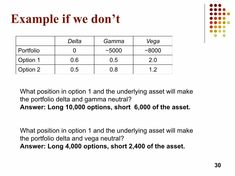
Example if we don’t
30
Delta Gamma VegaPortfolio 0 −5000 −8000Option 1 0.6 0.5 2.0Option 2 0.5 0.8 1.2
What position in option 1 and the underlying asset will make the portfolio delta and gamma neutral? Answer: Long 10,000 options, short 6,000 of the asset.
What position in option 1 and the underlying asset will make the portfolio delta and vega neutral? Answer: Long 4,000 options, short 2,400 of the asset.

Example if we do
31
Delta Gamma VegaPortfolio 0 −5000 −8000Option 1 0.6 0.5 2.0Option 2 0.5 0.8 1.2
What position in option 1, option 2, and the asset will make the portfolio delta, gamma, and vega neutral all at once?
We solve−5000 + 0.5w1 + 0.8w2 =0−8000 + 2.0w1 + 1.2w2 =0
to get w1 = 400 and w2 = 6,000. We therefore require long positions of 400 and 6,000 in option 1 and option 2.
However, because these additions result in an incremental positive delta of 400(0.6)+6,000(0.5)=3,240, we also need to take a short position of 3,240 in the asset in order to also make the portfolio delta neutral.

Rho
l Rho is the rate of change of the value of a derivative with respect to the interest rate.
l It is usually small and not a big issue in practice, unless the option is deep in-the-money and has a long horizon (discounting a larger cash flow over a longer horizon is more relevant then).
32

Hedging in Practice
l Traders usually ensure that their portfolios are delta-neutral at least once a day.
l Whenever the opportunity arises, they improve gamma and vega.
l As the portfolio becomes larger, hedging becomes less expensive since the trading cost per option goes down.
33

Scenario Analysis
l In addition to monitoring risks such as delta, gamma, and vega, option traders often also conduct a scenario analysis.
l A scenario analysis involves computing the gains and losses on the portfolio over a specified period of time under a variety of different scenarios.
l Often the two main sources of risk looked as variables (the scenarios) are the underlying asset price and volatility.
34
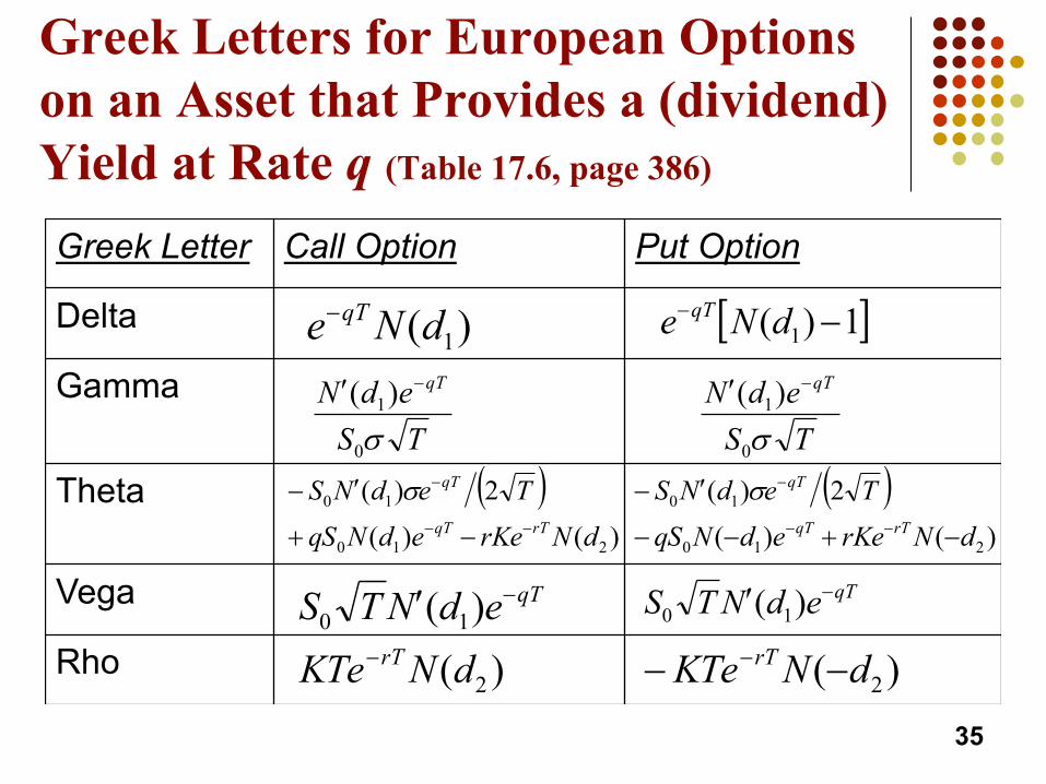
Greek Letters for European Options on an Asset that Provides a (dividend) Yield at Rate q (Table 17.6, page 386)
35
Greek Letter Call Option Put Option
Delta
Gamma
Theta
Vega
Rho
)( 1dNe qT-
TSedN qT
s01)( -¢
TSedN qT
s01)( -¢
[ ]1)( 1 -- dNe qT
( ))()(
2)(
210
10
dNrKeedNqSTedNSrTqT
qT
--
-
-+
¢- s ( ))()(
2)(
210
10
dNrKeedNqSTedNS
rTqT
qT
-+--
¢---
-s
qTedNTS -¢ )( 10qTedNTS -¢ )( 10
)( 2dNKTe rT- )( 2dNKTe rT -- -
Using Futures for Delta Hedging
l The delta of a futures contract on an asset paying a yield at rate q is e(r-q)T, since we know that F=Se(r-q)T.
l The position required in futures for delta hedging (instead of using the spot asset) is therefore e-(r-q)T times the position required in the corresponding spot asset.
36

Example of Using Futures for Delta Hedging (instead of the spot)
l A portfolio of currency options held by a US bank can be made delta neutral with a short position of 458,000 pounds sterling (of the spot (currency) asset, if it were used).
l If the US riskless rate is 4% and the UK rate 7%, hedging for 9 months using a short position in futures contracts instead of shorting the spot currency would require shorting:
e-(0.04-0.07)x9/12 x 458,000 or £468,422 in futures contracts.
l Since each futures contract is for £62,500 the number of contracts to be shorted is 468,422/62,500 = 7.49 contracts therefore rounded to 7 contracts.
37
Hedging vs. Creation of an Option Synthetically
l When we are hedging we take positions that offset delta, gamma, vega, etc…
l When we create an option synthetically we take positions that match delta, gamma, vega, etc…
38

Portfolio Insurance
l In October of 1987, many portfolio managers attempted to create a put option on a portfolio synthetically.
l This involves initially selling enough of the portfolio (or of index futures) to match the D of the put option.
39
Portfolio Insurance (continued)
l As the value of the portfolio increases, the D of the put becomes less negative and some of the original portfolio is repurchased.
l As the value of the portfolio decreases, the D of the put becomes more negative and more of the portfolio must be sold.
l The strategy did not work well on October 19, 1987 because since everyone was doing the same thing, liquidity became an issue.
l Additionally, investors that anticipated the portfolio insurers reaction sold their positions as well, exacerbating the problem and precipitating the price decrease, making the crash worse.
40