The Great Recession and the Inflation Puzzle

Troy Matheson and Emil Stavrev

WP/13/124

© 2013 International Monetary Fund WP/13/124 IMF Working Paper

Research Department

The Great Recession and the Inflation Puzzle

Prepared by Troy Matheson and Emil Stavrev

Authorized for distribution by Hamid Faruqee

May 2013

Abstract

This Working Paper should not be reported as representing the views of the IMF. The views expressed in this Working Paper are those of the author(s) and do not necessarily represent those of the IMF or IMF policy. Working Papers describe research in progress by the author(s) and are published to elicit comments and to further debate.

Notwithstanding persistently-high unemployment following the Great Recession, inflation in the United States has been remarkably stable. We find that a traditional Phillips curve describes the behavior of inflation reasonably well since the 1960s. Using a non-linear Kalman filter that allows for time-varying parameters, we find that three factors have contributed to the observed stability of inflation: inflation expectations have become better anchored and to a lower level; the slope of the Phillips curve has flattened; and the importance of import-price inflation has increased. JEL Classification Numbers: C53, E37 Keywords: Inflation, Unemployment, Phillips Curve Author’s E-Mail Address: tmatheson@imf.org; estavrev@imf.org

2

Contents Page

I. Introduction ............................................................................................................................3

II. Model and Estimation ...........................................................................................................3

A. Model ........................................................................................................................3 B. Data ...........................................................................................................................4 C. Non-linear Kalman Filter with State Constraints ......................................................4 D. Estimation .................................................................................................................5

III. Results ..................................................................................................................................6

IV. Conclusions..........................................................................................................................7 References ..................................................................................................................................8

3

I. INTRODUCTION1

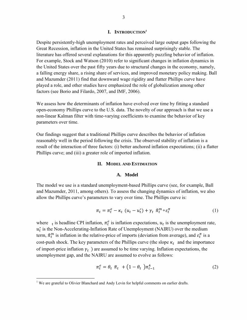
Despite persistently-high unemployment rates and perceived large output gaps following the Great Recession, inflation in the United States has remained surprisingly stable. The literature has offered several explanations for this apparently puzzling behavior of inflation. For example, Stock and Watson (2010) refer to significant changes in inflation dynamics in the United States over the past fifty years due to structural changes in the economy, namely, a falling energy share, a rising share of services, and improved monetary policy making. Ball and Mazumder (2011) find that downward wage rigidity and flatter Phillips curve have played a role, and other studies have emphasized the role of globalization among other factors (see Borio and Filardo, 2007, and IMF, 2006). We assess how the determinants of inflation have evolved over time by fitting a standard open-economy Phillips curve to the U.S. data. The novelty of our approach is that we use a non-linear Kalman filter with time-varying coefficients to examine the behavior of key parameters over time. Our findings suggest that a traditional Phillips curve describes the behavior of inflation reasonably well in the period following the crisis. The observed stability of inflation is a result of the interaction of three factors: (i) better anchored inflation expectations; (ii) a flatter Phillips curve; and (iii) a greater role of imported inflation.

II. MODEL AND ESTIMATION

A. Model

The model we use is a standard unemployment-based Phillips curve (see, for example, Ball and Mazumder, 2011, among others). To assess the changing dynamics of inflation, we also allow the Phillips curve’s parameters to vary over time. The Phillips curve is:

+

(1)

where is headline CPI inflation, is inflation expectations, is the unemployment rate,

is the Non-Accelerating-Inflation Rate of Unemployment (NAIRU) over the medium

term, is inflation in the relative-price of imports (deviation from average), and

is a cost-push shock. The key parameters of the Phillips curve (the slope and the importance of import-price inflation are assumed to be time varying. Inflation expectations, the unemployment gap, and the NAIRU are assumed to evolve as follows:

(2)

1 We are grateful to Olivier Blanchard and Andy Levin for helpful comments on earlier drafts.

4

(3)

with:

(4) where is long-run inflation expectations,

is year-over-year headline CPI inflation (lagged one quarter), and is a time-varying weight attached to long-run inflation expectations that reflects the stability of inflation expectations. The parameters ( , , ) are assumed to be constrained random walks ( and and ), while , the persistence of the unemployment gap, is assumed to be constant ( ).

B. Data

The data are measured at the quarterly frequency and are seasonally adjusted. The sample period covers 1961Q1 to 2012Q2. The relative price of imports is the import-price deflator relative to the GDP deflator. All inflation rates are annualized. The series for long-run inflation expectations is sourced from the Federal Reserve Bank Board.

C. Non-linear Kalman Filter with State Constraints

Because our Phillips curve is non-linear in the parameters, we employ a non-linear, extended Kalman filter (see Civera and Others, 2011). The Kalman filter is:

(5)

(6) where represents the state equations (in our case, , represents the measurement equations, and is a non-linear differentiable function. The forward recursions of the filter are:

Prediction State

Covariance

Update Measurement

Covariance

Kalman Gain

State

Covariance

5

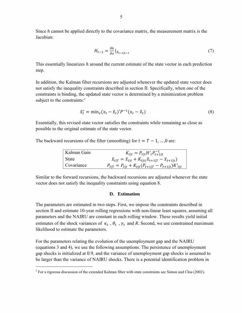
Since h cannot be applied directly to the covariance matrix, the measurement matrix is the Jacobian:

(7) This essentially linearizes around the current estimate of the state vector in each prediction step. In addition, the Kalman filter recursions are adjusted whenever the updated state vector does not satisfy the inequality constraints described in section II. Specifically, when one of the constraints is binding, the updated state vector is determined by a minimization problem subject to the constraints:2

(8) Essentially, this revised state vector satisfies the constraints while remaining as close as possible to the original estimate of the state vector. The backward recursions of the filter (smoothing) for are:

Kalman Gain

State Covariance

Similar to the forward recursions, the backward recursions are adjusted whenever the state vector does not satisfy the inequality constraints using equation 8.

D. Estimation

The parameters are estimated in two steps. First, we impose the constraints described in section II and estimate 10-year rolling regressions with non-linear least squares, assuming all parameters and the NAIRU are constant in each rolling window. These results yield initial estimates of the shock variances of , and Second, we use constrained maximum likelihood to estimate the parameters. For the parameters relating the evolution of the unemployment gap and the NAIRU (equations 3 and 4), we use the following assumptions. The persistence of unemployment gap shocks is initialized at , and the variance of unemployment gap shocks is assumed to be larger than the variance of NAIRU shocks. There is a potential identification problem in 2 For a rigorous discussion of the extended Kalman filter with state constraints see Simon and Chia (2002).

6

determining the relative variance of unemployment gap and NAIRU shocks, the signal-to-noise ratio . Thus, for robustness, we calibrate two different versions of the model, one where the NAIRU is assumed to be relatively stable ( ) and one where it is relatively flexible ( ). Imposing the signal-to-noise ratio allows us to reduce the number parameters to be estimated by one. Our final assumption relates to how far the maximum likelihood estimates of the shock variances can deviate from the initial conditions explained above. Essentially, we restrict the shock variances to be less than or equal to those obtained from rolling regressions. This guarantees that the variability of the parameters is constrained relative to the estimates from the rolling regressions while maximizing the fit of the Phillips curve (i.e. the variance of cost-push shocks is strictly lower than the average shock variance obtained from rolling regressions).3

III. RESULTS

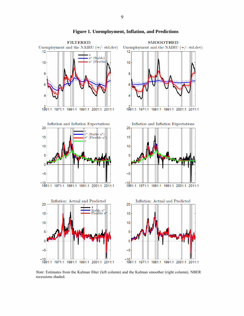
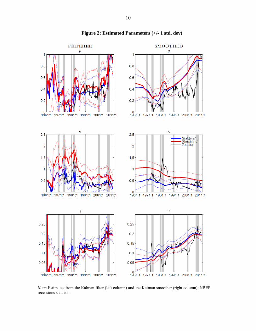
Figure 1 displays the one-quarter-ahead predictions (filtered) and the full-sample estimates (smoothed) of the NAIRU, inflation expectations, and the predicted values of the Phillips curve. We find that the results are qualitatively very similar for the filtered and smoothed estimates, irrespective of whether the NAIRU is assumed to be stable or flexible. Moreover, with exception of a handful of episodes with particularly large inflation spikes, the Phillips curve fits the data reasonably well. The results show that long-run inflation expectations became unanchored during the 1970s while inflation expectations became more backward looking and volatile. As the Federal Reserve began moving toward inflation targeting in the early 1980s, long-run inflation expectations began drifting downward and eventually settled at a lower level (around 2 percent) around 2000. Figure 2 shows the evolution of the parameters over time, along with estimates from the rolling regressions. We find the short-run inflation expectations have become more stable ( has increased) and remained remarkably stable in the several years following the Great Recession. At the same time, the slope of the Phillips curve has flattened over time and, at the end of sample (mid-2012), is roughly half the magnitude it was in the 1970s. The observed flattening of the Phillips curve is very similar across different specifications of the NAIRU. Note, however, the level of the slope is higher when a more flexible NAIRU is assumed. This is perhaps not surprising, and serves as reminder of the difficulty in uniquely

3 The empirical findings are qualitatively very similar if the shock variances are assumed to be strictly larger than those obtained from rolling regressions. These results are available from the authors on request.

7

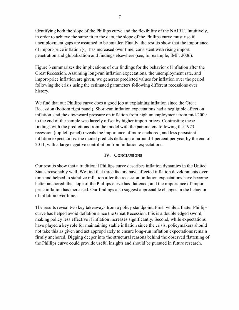
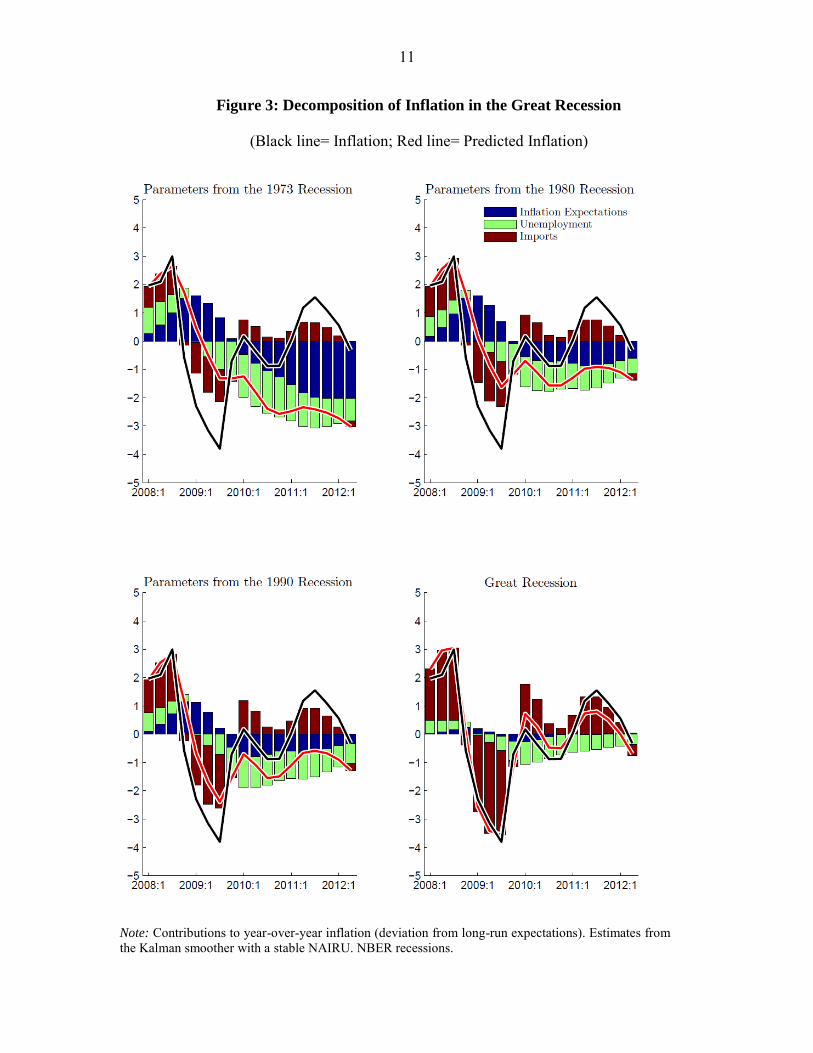
identifying both the slope of the Phillips curve and the flexibility of the NAIRU. Intuitively, in order to achieve the same fit to the data, the slope of the Phillips curve must rise if unemployment gaps are assumed to be smaller. Finally, the results show that the importance of import-price inflation has increased over time, consistent with rising import penetration and globalization and findings elsewhere (see, for example, IMF, 2006). Figure 3 summarizes the implications of our findings for the behavior of inflation after the Great Recession. Assuming long-run inflation expectations, the unemployment rate, and import-price inflation are given, we generate predicted values for inflation over the period following the crisis using the estimated parameters following different recessions over history. We find that our Phillips curve does a good job at explaining inflation since the Great Recession (bottom right panel). Short-run inflation expectations had a negligible effect on inflation, and the downward pressure on inflation from high unemployment from mid-2009 to the end of the sample was largely offset by higher import prices. Contrasting these findings with the predictions from the model with the parameters following the 1973 recession (top left panel) reveals the importance of more anchored, and less persistent inflation expectations: the model predicts deflation of around 1 percent per year by the end of 2011, with a large negative contribution from inflation expectations.

IV. CONCLUSIONS

Our results show that a traditional Phillips curve describes inflation dynamics in the United States reasonably well. We find that three factors have affected inflation developments over time and helped to stabilize inflation after the recession: inflation expectations have become better anchored; the slope of the Phillips curve has flattened; and the importance of import-price inflation has increased. Our findings also suggest appreciable changes in the behavior of inflation over time. The results reveal two key takeaways from a policy standpoint. First, while a flatter Phillips curve has helped avoid deflation since the Great Recession, this is a double edged sword, making policy less effective if inflation increases significantly. Second, while expectations have played a key role for maintaining stable inflation since the crisis, policymakers should not take this as given and act appropriately to ensure long-run inflation expectations remain firmly anchored. Digging deeper into the structural reasons behind the observed flattening of the Phillips curve could provide useful insights and should be pursued in future research.

8

REFERENCES

Civera Javier, Andrew T. Davidson, and Jose Maria Martinez Montiel, 2011, Structure from

Motion Using the Extended Kalman Filter (Berlin: Springer Verlag). Laurence Ball and Sandeep Mazumder, 2011, “Inflation Dynamics and the Great Recession,”

Brookings Papers on Economic Activity, Vol. 42, Spring, pp. 337–405. IMF, 2006, “How Has Globalization Affected Inflation?” IMF World Economic Outlook,

April, Chapter 3. Simon Dan and Tien Li Chia, 2002, “Kalman Filtering with State Equality Constraints,”

IEEE Transactions on Aerospace and Electronic Systems, Vol. 38, Number 1, pp. 128–136.

James Stock and Mark Watson, 2010, “Modeling Inflation After the Crisis,” FRB Kansas

City Symposium, Jackson Hole, Wyoming.

9

Figure 1. Unemployment, Inflation, and Predictions

Note: Estimates from the Kalman filter (left column) and the Kalman smoother (right column). NBER recessions shaded.

10

Figure 2: Estimated Parameters (+/- 1 std. dev)

Note: Estimates from the Kalman filter (left column) and the Kalman smoother (right column). NBER recessions shaded.

11

Figure 3: Decomposition of Inflation in the Great Recession

(Black line= Inflation; Red line= Predicted Inflation)

Note: Contributions to year-over-year inflation (deviation from long-run expectations). Estimates from the Kalman smoother with a stable NAIRU. NBER recessions.