The Great Intervention and Massive Money Injection:The Japanese Experience 2003-2004

Tsutomu WatanabeAnd

Tomoyoshi Yabu

June 11, 2007

JSPS Grants-in-Aid for Creative Scientific ResearchUnderstanding Inflation Dynamics of the Japanese Economy

Working Paper Series No.12

Research Center for Price DynamicsInstitute of Economic Research, Hitotsubashi University

Naka 2-1, Kunitachi-city, Tokyo 186-8603, JAPANTel/Fax: +81-42-580-9138

E-mail: sousei-sec@ier.hit-u.ac.jphttp://www.ier.hit-u.ac.jp/~ifd/

The Great Intervention and Massive Money Injection:

The Japanese Experience 2003-2004

Tsutomu Watanabe∗

Hitotsubashi UniversityTomoyoshi YabuBank of Japan

June 6, 2007

Abstract

From the beginning of 2003 to the spring of 2004, Japan’s monetary authorities conductedlarge-scale yen-selling/dollar-buying foreign exchange operations in what Taylor (2006) has la-beled the “Great Intervention.” The purpose of the present paper is to empirically examine therelationship between this “Great Intervention” and the quantitative easing policy the Bank ofJapan (BOJ) was pursuing at that time. Using daily data of the amount of foreign exchangeinterventions and current account balances at the BOJ, our analysis arrives at the following con-clusions. First, while about 60 percent of the yen funds supplied to the market by yen-sellinginterventions were immediately offset by the BOJ’s monetary operations, the remaining 40 percentwere not offset and remained in the market for some time; this is in contrast with the precedingperiod, when almost 100 percent were offset. Second, comparing foreign exchange interventionsand other government payments, the extent to which the funds were offset by the BOJ were muchsmaller in the case of foreign exchange interventions, and the funds also remained in the marketlonger. This finding suggests that the BOJ differentiated between and responded differently toforeign exchange interventions and other government payments. Third, the majority of financingbills issued to cover intervention funds were purchased by the BOJ from the market immediatelyafter they were issued. For that reason, no substantial decrease in current account balances linkedwith the issuance of FBs could be observed. These three findings indicate that it is highly likelythat the BOJ, in order to implement its policy target of maintaining current account balances ata high level, intentionally did not sterilize yen-selling/dollar-buying interventions.

JEL Classification Numbers : F30; E52; E58Keywords: foreign exchange intervention; sterilization; quantitative easing

∗Correspondence: Tsutomu Watanabe, Institute of Economic Research, Hitotsubashi University, Kunitachi, Tokyo186-8603, Japan. Phone: 81-42-580-8358, fax: 81-42-580-8333, e-mail: tsutomu.w@srv.cc.hit-u.ac.jp. We would like tothank Takatoshi Ito and Masaaki Shirakawa for useful conversations.

1 Introduction

During the period from 2001 to 2006, the Japanese monetary authorities pursued two important and

very interesting policies. The first of these is the quantitative easing policy introduced by the Bank of

Japan (BOJ) in March 2001. This step was motivated by the fact that although the overnight call rate,

the BOJ’s policy rate, had reached its lower bound at zero percent, it failed to sufficiently stimulate

the economy. To achieve further monetary easing, the BOJ therefore changed the policy variable

from the interest rate to the money supply. The quantitative easing policy remained in place until

March 2006, by which time the Japanese economy had recovered. The second major policy during

this period were interventions in the foreign exchange market by Japan’s Ministry of Finance (MOF),

which engaged in large-scale selling of the yen from January 2003 to March 2004. Taylor (2006) has

called this the “Great Intervention.” The interventions during this period occurred at a frequency of

once every two business days, with the amount involved per daily intervention averaging Y286 billion

and the total reaching Y35 trillion. Even for Japan’s monetary authorities, which are known for their

active interventionism, this frequency as well as the sums involved were unprecedented.

The main concern of this paper is to examine how these two policies were related to each other.

In general, monetary policy and exchange rate interventions are independent policies and, as is often

pointed out, not mutually related.1 With the important exception of Japan since 2001, monetary

policy in major economies such as the United States and Europe is conducted by setting a target

level for very short-term interest rates (e.g., the Federal funds rate in the US, the overnight call

rate in Japan) and adjusting the quantity of base money on a daily basis to maintain that level.

Therefore, if the amount of yen funds circulating in the market increases or decreases as a result of

foreign exchange market interventions, overnight interest rates will diverge from the target level.2 In a

sterilized intervention, the central bank will then use open market operations to offset the funds in the

domestic currency supplied to or absorbed from the market by the foreign exchange intervention. It

is said that in practice, the central banks of the advanced economies always sterilize foreign exchange

1See, for example, Craig and Humpage (2001).2In order to conduct foreign exchange interventions in which yen are sold and dollars are bought, the MOF has to

supply yen funds. One way to do so is to issue financing bills (FBs) on the same day as the intervention is conducted. Inthat case, because the MOF immediately returns the yen funds that it obtained by issuing FBs to the market throughthe intervention, the amount of yen funds circulating in the market does not change. However, in practice, there is atime gap of about two months between foreign exchange market interventions and the issuing of FBs; as a result, if theMOF intervenes by selling yen, the amount of yen funds circulating at that point in time actually increases. For detailson the practicalities of foreign exchange market interventions in Japan, see Ito (2003).

2

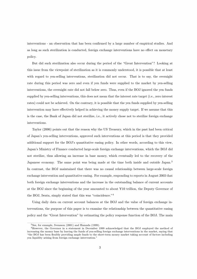
interventions - an observation that has been confirmed by a large number of empirical studies. And

as long as such sterilization is conducted, foreign exchange interventions have no effect on monetary

policy.

But did such sterilization also occur during the period of the “Great Intervention”? Looking at

this issue from the viewpoint of sterilization as it is commonly understood, it is possible that at least

with regard to yen-selling interventions, sterilization did not occur. That is to say, the overnight

rate during this period was zero and even if yen funds were supplied to the market by yen-selling

interventions, the overnight rate did not fall below zero. Thus, even if the BOJ ignored the yen funds

supplied by yen-selling interventions, this does not mean that the interest rate target (i.e., zero interest

rates) could not be achieved. On the contrary, it is possible that the yen funds supplied by yen-selling

intervention may have effectively helped in achieving the money supply target. If we assume that this

is the case, the Bank of Japan did not sterilize, i.e., it actively chose not to sterilize foreign exchange

interventions.

Taylor (2006) points out that the reason why the US Treasury, which in the past had been critical

of Japan’s yen-selling interventions, approved such interventions at this period is that they provided

additional support for the BOJ’s quantitative easing policy. In other words, according to this view,

Japan’s Ministry of Finance conducted large-scale foreign exchange interventions, which the BOJ did

not sterilize, thus allowing an increase in base money, which eventually led to the recovery of the

Japanese economy. The same point was being made at the time both inside and outside Japan.3

In contrast, the BOJ maintained that there was no causal relationship between large-scale foreign

exchange intervention and quantitative easing. For example, responding to reports in August 2003 that

both foreign exchange interventions and the increase in the outstanding balance of current accounts

at the BOJ since the beginning of the year amounted to about Y10 trillion, the Deputy Governor of

the BOJ, Iwata, simply stated that this was “coincidence.”4

Using daily data on current account balances at the BOJ and the value of foreign exchange in-

terventions, the purpose of this paper is to examine the relationship between the quantitative easing

policy and the “Great Intervention” by estimating the policy response function of the BOJ. The main

3See, for example, Svensson (2001) and Hamada (1999).4However, the Governor in a statement in December 1999 acknowledged that the BOJ employed the method of

increasing the money base by leaving the funds of yen-selling foreign exchange interventions in the market, saying that“the BOJ has been flexibly providing ample funds to the short-term money market taking account of factors includingyen liquidity arising from foreign exchange intervention.”

3

finding of this investigation is that around 60 percent of the yen funds supplied to the market by

yen-selling interventions were offset by monetary adjustments by the BOJ (i.e., sterilized), while the

remaining 40 percent were not offset. Moreover, the funds that were not offset remained in the market

for quite a while. As a result, in contrast with the preceding period when nearly 100 percent were offset,

during the quantitative easing period, the extent to which interventions were not sterilized increased

remarkably.5 During the “Great Intervention,” interventions totaling Y35 trillion were implemented,

while the outstanding balance of current accounts during this period rose from approximately Y20

trillion to Y33.7 trillion. What is interesting is that this increase in current account balances of Y13

trillion is roughly equivalent to 40 percent of the value of foreign exchange interventions and thus

virtually coincides with our estimation result. The results of this paper thus show that it is highly

likely that the BOJ intentionally did not sterilize yen-selling/dollar-buying interventions in order to

realize its policy goal of maintaining the outstanding balance of current accounts at a high level.

The remainder of this paper is organized as follows. The next section explains the quantitative

easing policy and the “Great Intervention” in greater detail. Section 3 investigates the correlation

between interventions and changes in current account balances at the BOJ, while Section 4 estimates

the policy response function of the BOJ. Finally, Section 5 concludes.

2 The Quantitative Easing Policy and the “Great Interven-

tion”

2.1 The quantitative easing policy

The BOJ decided to introduce its quantitative easing policy on March 19, 2001 (see Table 1 for a

chronology of monetary policy measures in Japan).6 The aim of this policy was to stimulate effective

demand by providing ample supplies of base money. The target level of outstanding current account

balances at the BOJ was initially set at Y5 trillion, meaning that the target level exceeded the level

of required reserve, which was approximately Y4 trillion, by about Y1 trillion.

As indicated, the main purpose of this paper is to examine how the BOJ decided the level of current

5Empirical investigations on the sterilization operations of the BOJ during this period can be found, among others,in Ito (2004), Fatum and Hutchison (2005), and Spiegel (2003). However, these studies do not explicitly formulate apolicy response function and therefore do not provide firm evidence that interventions were not sterilized.

6The BOJ adopted its zero interest rate policy aiming to keep the target level of the overnight interest rate at zeroin February 1999 and maintained this until August 2000. Although the zero interest rate policy and the quantitativeeasing policy have in common that they aim to maintain the overnight interest rate at zero, the latter differs in the waythat it affects aggregate demand not through the interest rate channel.

4

account balances on a daily basis and the relationship this had with foreign exchange interventions.

In this context, two important features of the quantitative easing policy need to be highlighted. The

first of these is that there were frequent adjustments of the target level of current account balances.

After the initial level had been set at Y5 trillion in March 2001, this was raised to Y6 trillion less than

half a year later, in August 2001. By December of that year, the target level was further increased

to a range of Y10-15 trillion, and this range continued to be raised at relatively short intervals until

it finally reached Y30-35 trillion in January 2004. Thus, what is important is not only that current

account balances were at a high level, but also that they continued to increase.

Second, since December 2001, the target for current account balances was no longer a point value

but a range. For example, in January 2004, the range was set at Y30-35 trillion, meaning that

fluctuations up to Y5 trillion were acceptable. Although the BOJ has not explained why it set a

target range or on what basis it decided that this range would be Y5 trillion, looking at the BOJ’s

actual monetary policy conduct (Figure 1), it becomes clear that in practice it permitted fluctuations

within this range. This pattern is especially obvious in the period since 2003, the main period of

interest for this paper.

In order to examine this point in greater detail, Figure 2 depicts the distribution of the actual values

of daily current account balances during the period when the target range was Y30-35 trillion, i.e.,

from January 2004 to March 2006. It shows that the mode of the distribution is at Y33.7 trillion and

the frequency declines toward the fringes of the range. Thus, it can be conjectured that even though in

the daily operation of monetary policy, the BOJ had set a provisional target level of Y33.7 trillion, it

was prepared to accept divergences from that level at times of large autonomous disturbances through

the inflow and outflow of funds, etc.

2.2 The “Great Intervention”

Figure 3 shows the value of foreign exchange interventions between 2001 and 2007. As can be seen,

the pattern of interventions is quite remarkable, showing a high frequency of interventions during the

period from January 15, 2003 to March 16, 2004. As is well-known, it is the Ministry of Finance, and

in particular the Vice Minister of Finance for International Affairs, who plays a leading role in foreign

exchange interventions, and it is conspicuous that interventions were concentrated in the period when

Zembei Mizoguchi was in this post. Compared with the period of his predecessors, Sakakibara and

5

Kuroda (who held the post between June 1995 and January 2002), the frequency of interventions

increased remarkably from, on average, once every forty days to once every two days. Moreover,

whereas the total amount of interventions under Sakakibara and Kuroda came to Y26 trillion, under

Mizoguchi it reached Y35 trillion, providing further indication of the heavy intervention during a short

period.

3 The Correlation Between Interventions and Changes in Cur-

rent Account Balances

We now turn to examining whether there is a correlation between changes in current account balances

and foreign exchange interventions. If there is a positive correlation between the two, this would mean

that foreign exchange interventions were not sterilized. Conversely, no correlation would mean that

interventions were sterilized.

In order to examine this issue, let us begin by examining the relationship between the two with

a simple scattergram. Figure 4 plots daily data with the horizontal axis depicting the value of inter-

ventions and the vertical axis showing the change in current account balances. The sample consists of

observations from 1992 onward and is divided into the periods before and after December 19, 2001, the

date on which the BOJ first set a target range for current account balances. Current account balances

at the end of day t are denoted by Rt, while the value of yen sales/dollar purchases conducted on day

t is denoted by It. The vertical axis shows 4Rt, while the horizontal axis depicts It−2. The value ofinterventions at t− 2 is used because the settlement of funds typically takes place two business daysafter interventions were executed.

As can be see from Figure 4, there is almost no correlation between the two in the first half of the

observation period. In contrast, in the latter half of the observation period, a weak correlation can

be observed. We examine this difference using a simple regression analysis, estimating the following

equation for each period:

4Rt = µ+ βIt−2 + ut (1)

The results of the regression are shown in Table 2. As for the first period, we find that the estimated

value of β at -0.004 is extremely small and we cannot reject the null hypothesis of β = 0. In other

words, we cannot reject the hypothesis that interventions during this period were completely sterilized.

6

In contrast, for the latter period, at 0.389, β is positive and statistically significant, suggesting that

approximately 60 percent of the value of foreign exchange interventions was sterilized, while the

remaining 40 percent was not. During the period of the “Great Intervention” (from January 2003 to

March 2004), foreign exchange interventions totaling Y35 trillion were carried out. At the same time,

current account balances at the BOJ during this period increased from Y20 trillion to Y33 trillion.

Interestingly, the increase in current account balances of Y13 trillion is equivalent to approximately

40 percent of the value of foreign exchange interventions. Thus the estimation result and the actual

figure are almost identical.

The results presented in Table 2 suggest that it is possible that the correlation between inter-

ventions and changes in current account balances may differ depending on the observation period.

Therefore, we use equation (1) to conduct a rolling regression in order to examine the change in the

coefficient β over time. The window of the rolling regression is the preceding 750 days. The results are

shown in Figure 5, which shows the estimated value of β as well as the 90 percent confidence interval.

The figure indicates that while until 2000, β is zero or below zero, it turns positive in September 2001

and from March 2003 onward becomes large and significantly different from zero. Moreover, after

2003, the value of β is relatively stable at around 0.4.

4 Estimation of the Policy Response Function

Equation (1) represents an estimation equation that has been widely used in preceding studies to

measure the extent of sterilization. Examining the most recent period in Japan, Fatum and Hutchison

(2005) and Ito (2004), for example, employed a similar specification. However, estimating the conduct

of the BOJ during the period of quantitative easing poses the following serious problems.

First, even if there was a positive correlation between interventions and changes in current account

balances, such a correlation may be spurious. To illustrate this, let us consider the case where current

account balances are at the lower limit of the target range. The BOJ may want to return current

account balances to the middle of the target range and is planning operations to supply the market with

funds. Let us further assume that at this moment, the Ministry of Finance conducts a yen-selling

intervention that was unexpected for the BOJ. Then, because current account balances approach

the middle of the target range as a result of the supply of funds to the market via the yen-selling

intervention, the BOJ may decide to abandon its planned operation and leave the funds from the

7

intervention in the market. In such cases, it is possible to observe a positive correlation between

interventions and changes in current account balances. However, such a correlation is spurious and

does not represent non-sterilization. In order to overcome this problem, it is necessary to estimate a

specification that explicitly takes into account how the BOJ changes current account balances within

the target range.

Second, equation (1) only looks at the correlation between interventions and the change in current

account balances on the specific day on which interventions are settled. Even if the correlation between

interventions and changes in current account balances on that specific day is high, it is possible that

the relationship weakens with the passage of time. For example, interventions often come unexpected

for the central bank and for that reason it is difficult to conduct operations to immediately sterilize

an intervention. Another reason why sterilization may not occur on the day of the intervention is to

avoid that market participants know that the intervention has taken place. In this case, the central

bank may allow current account balances to change in response to the intervention on the settlement

day, but may then conduct operations on the next day, or the day after that, to return current account

balances to their original level. In other words, looked at not from any particular moment in time but

from a dynamic perspective, it is possible that interventions have been sterilized.

Third, even if the estimation results of equation (1) were to show non-sterilization, this does not

necessarily mean that the BOJ discriminated between interventions and other government payments

and responded differently. The government pays funds to the private sector, for example in the form of

pension payments, and also receives funds, such as in the form of taxes. The supply of yen funds to the

market through yen-selling/dollar-buying interventions represents one way in which the government

pays part of its funds. If the central bank generally does not sterilize government payments, including

those in the form of foreign exchange interventions, this would not be a particularly interesting finding.

What we are interested in is whether or not the central bank distinguishes between foreign exchange

interventions and other government payments and increases the degree of non-sterilization in the case

of foreign exchange interventions. In order to examine this, it is not enough to only look at the

correlation between interventions and changes in current account balances; instead, it is necessary

to also estimate the correlation between other government payments and changes in current account

balances and then to compare the two correlations.

8

4.1 The target range of current account balances

We now turn to the estimation of the central bank’s policy response function taking the above three

points into consideration. We begin by modeling how the BOJ adjusted current account balances

within the target range. In the first specification, the BOJ aims for a specific level within the target

range and conducts daily operations to steer balances as far as possible toward that level. In this case,

equation (1) should be extended as follows:

Rt = µ+ ρRt−1 + βIt−2 + ut (2)

where ρ is the parameter for the adjustment speed to the desired level and satisfies |ρ| < 1. The closerρ is to 1, the slower is the convergence to the desired level.

In equation (2), the central bank tries to steer current account balances toward the desired level

even if they are within the target range. However, another possibility is that the central bank allows

current account balances to fluctuate freely as long as they are within the target range and only tries

to steer them to the target range when they move outside it. In this case, equation (1) should be

extended as follows:

Rt = µ+ ρRt−1 + ρ∗R∗t−1 + βIt−2 + ut (3)

where the variable R∗t is defined as R∗t ≡ Rt ∗ 1[Rt > Ruppert or Rt < Rlowert ] (where Ruppert stands

for the upper limit of the target range and Rlowert for the lower limit). That is, R∗t equals to Rt

when Rt is within the target range; otherwise it equals to zero. Equation (3) implies that when Rt is

within the target range, it converges to the desired level with speed 1− ρ, while when it is outside thetarget range, it converges with speed 1 − (ρ+ ρ∗). For example, if the BOJ permits current account

balances to move freely within the target range and there is no convergence whatsoever, but once

current account balances are outside the range, they converge to the desired level, this means that

ρ = 1 and −2 < ρ∗ < 0.

The estimation results for equations (2) and (3) are shown in Table 3.7 In the estimation, dummy

variables for a change in the target for current accounts were added to both equations.8

7The estimation period for equation (2) is from December 2001, when the BOJ first set a target range for currentaccount balances, to March 2006, when the quantitative easing policy ended. In contrast, the estimation period forequation (3) begins in May 2003, when the target range was set to Y27-30 trillion.

8Specifically, six dummy variables for the following dates were included: 2002/10/30, 2003/4/1, 2003/4/30,2003/5/20, 2003/10/10, and 2004/1/20. Each dummy variable takes a value of one from that date onward.

9

In equation (2), the estimation result for ρ is 0.819, meaning that when current account bal-

ances diverge from the desired level, the time required to halve that divergence is 3.5 days (≈ln(0.5)/ ln(0.819)). In other words, convergence is quite rapid. The estimated value of β, the pa-

rameter of main concern for the investigation here, is 0.405, which is only slightly larger than the

result obtained in Table 2. From these estimation results, we can conclude that the correlation be-

tween foreign exchange interventions and changes in current account balances is not spurious. Next,

looking at the estimation results for equation (3), the estimated value of ρ is 0.646 and that of ρ∗ is

-0.012, indicating that the difference in the speed of convergence outside and within the target range

is not that great. Moreover, the estimated value of β is 0.460, showing a high degree of sterilization.

4.2 The dynamic effects of foreign exchange interventions

To consider the dynamic effects of foreign exchange interventions, let us further expand equation (2)

in the following manner:

Rt = µ+ ρRt−1 +KXk=0

βkIt−2−k + ut (4)

Unlike equation (2), this specification makes it possible to consider the impact on current account

balances not only of interventions two days earlier, but also of interventions three, four, or more days

earlier. In the estimation, dummy variables for a change in the target level of current accounts were

included.

Using the estimation results from equation (4), Figure 6 shows the effect of a Y1 trillion foreign

exchange intervention on current account balances.9 The estimation period is December 19, 2001 to

March 9, 2006. In the estimation, we set K = 9. The figure suggests that the effect at t of the

intervention, which was executed at t− 2, is about 0.5 and gradually declines thereafter and becomeszero at t+3; however, from t+7 onward it returns to around 0.4. This confirms that the unsterilization

of foreign exchange interventions is not an instantaneous phenomenon that occurs only at t.10

9Specifically, the effect of intervention at t−2 upon current account balances at t+j was calculated as β0+β1+· · ·+βj .10Another study examining the sterilization of interventions from a dynamic perspective is that by Fatum and Hutchi-

son (2005) who use the same data as this study and conclude that interventions are almost completely sterilized. How-ever, in contrast with the present study, their analysis does not take into account factors such as the lag betweeninterventions and the settlement of funds; moreover, it also differs from the present analysis in that changes in theconvergence of Rt to the desired level are not considered.

10

4.3 Comparison with government financial transactions other than foreignexchange interventions

In addition to foreign exchange interventions, the balance of current accounts at the BOJ also varies

as a result of the financial activities of the government. For example, when the government makes

pension payments to the private sector, current account balances increases. Conversely, when the

government collects taxes from the private sector, current account balances decrease.

Let the payment of government funds on day t be denoted by GPt, while government receipts are

denote by GRt11. Note that while yen-selling/dollar-purchasing interventions are normally included

in government payments, let GPt here denote only government payments other than foreign exchange

interventions. Using this definition of variables, equation (3) is expanded to yield the following esti-

mation equation:

Rt = µ+ [ρRt−1 + ρ∗R∗t−1] + [βIt−2 + β∗I∗t−2] + [γGPt + γ∗GP ∗t ] + [δGRt + δ∗GR∗t ] + ut (5)

Equation (5) differs from equation (3) in the following ways. First, government payments other

than foreign exchange interventions are explicitly considered as an explanatory variable. If the BOJ

does not distinguish between interventions and other government payments, then β and γ should take

the same value. In contrast, if the BOJ does distinguish between interventions and other government

payments and only leaves interventions unsterilized, β should be positive, while γ should be zero.

Second, equation (5) distinguishes whether current account balances move outside the target range

as a result of government payments and receipts or not. Specifically, I∗t , GP∗t , andGR

∗t are respectively

defined as follows:

I∗t ≡ It 1[Rt−1 + It > Ruppert ];

GP ∗t ≡ GPt 1[Rt−1 +GPt > Ruppert ]; (6)

GR∗t ≡ GRt 1[Rt−1 +GRt < Rlowert ]

where I∗t represents the case where current account balances exceed the upper limit of the target

range as a result of intervention. GP ∗t and GR∗t represent the corresponding cases for government

payments and government receipts. If the BOJ more strongly offsets large shocks in which current

account balances shoot out of the target range, β∗, γ∗, and δ∗ should take negative values.

11GPt and GRt are defined as GPt ≡ Gt1(Gt > 0) and GRt ≡ Gt1(Gt < 0)

11

The estimation results for equation (5) are presented in Table 4 and show the following. First,

looking at the response in current account balances to foreign exchange interventions, the estimated

value for β is 0.545 and that for β∗ is -0.465, indicating that when current account balances remained

within the target range despite foreign exchange interventions, more than 50 percent of the value of

such interventions were not sterilized, which is in line with earlier results. However, in the case of

large foreign exchange interventions that would lead current account balances to shoot outside the

target range, the impact is actually almost zero (β+β∗ = 0.08), meaning that such interventions were

almost completely sterilized.

Second, looking at the impact of government payments other than foreign exchange interventions

on current account balances, the estimated values of γ is 0.396 and that of γ+γ∗ is 0.208. Comparing

β and γ, the former is significantly larger than the latter, indicating that the extent to which foreign

exchange interventions are offset is smaller than the extent to which other government payments are

offset. However, the opposite is true when current account balances shoot outside target range; i.e.,

in this case, the extent to which government payments (other than foreign exchange interventions)

are offset is smaller than the extent to which foreign exchange interventions are offset.

Third, looking at the impact of government receipts on current account balances, the estimated

value of δ is 0.162 and that of δ + δ∗ is 0.268, indicating that with regard to a shock resulting in

current account balances shooting outside the target range, the extent to which this is offset is rather

small. Since offsetting a shock that leads to current account balances shooting below the lower limit

of the target range required the BOJ to supply funds by purchasing bonds from the market, this result

suggests that such purchasing operations may have been technically difficult in a situation where bond

yields were very close to the zero lower bound.12

Next, using equation (5), let us examine the dynamic effect of government payments including

foreign exchange interventions and government receipts on current account balances. The estimation

equation looks as follows:

Rt = µ+ [ρRt−1 + ρ∗R∗t−1] +KXk=0

[βkIt−2−k + β∗kI∗t−2−k] +

KXk=0

[γkGPt−k + γ∗kGP∗t−k]

+KXk=0

[δkGRt−k + δ∗kGR∗t−k] + ut (7)

The estimation results are displayed in Figure 7 and suggest the following. First, although the12For details on the situation of funds-supplying operations at that time, see Bank of Japan (2004).

12

effect of foreign exchange interventions gradually declines until t+4, it then remains relatively stable

at around 0.4 after that. This result is in contrast with the result shown in Figure 6, where the effect

disappears at t+ 3 and t+ 4. It probably reflects the correction of estimation bias as a result of the

explicit inclusion of government payments and receipts other than foreign exchange interventions as

explanatory variables. Second, comparing the effects of government payments and receipts, the effect

of payments becomes insignificant from the third day onward, while receipts have a positive effect all

the way through to the tenth day. This pattern also holds in the case where current account balances

shoot outside the target range.

Okina and Shiratsuka (2000) argue that because the yen funds required for yen-selling/dollar-

buying intervention will in any case eventually be obtained through the issuance of FBs, interventions

are always 100 percent sterilized. Generally, the issuance of FBs does not take place at the same time

as foreign exchange interventions but occurs about two months later. Therefore, according to their

argument, interventions will be sterilized after a period of two months. However, there is no guarantee

that the BOJ will remain inactive at the time when funds are absorbed from the market through the

issuance of FBs, since it may purchase FBs from the market at the same time that the government

issues FBs. If this were the case, the intervention will not be sterilized even from a dynamic viewpoint.

Consequently, in order to see whether an intervention was sterilized or not, it is necessary to examine

whether there is an increase in current account balances at the time that the government issued FBs.

To this end, we define FBt as the negative value of FBs issued and GRt as the receipt of government

funds except FBs and expand equation (9) as follows:

Rt = µ+ [ρRt−1 + ρ∗R∗t−1] +KXk=0

[βkIt−2−k + β∗kI∗t−2−k] +

KXk=0

[γkGPt−k + γ∗kGP∗t−k]

+

KXk=0

[δkGRt−k + δ∗kGR∗t−k] +

KXk=0

[ζkFBt−k + ζ∗kFB∗t−k] + ut (8)

Using the estimation result from equation (10), Figure 8 depicts the change in current account

balances associated with the issuance of Y1 trillion worth of FBs. Even though current account bal-

ances decrease on the day that FBs are issued, the effect on current account balances disappears after

three days and is no longer significant. This is a noteworthy trend when compared with government

receipts (GRt): while the impact of GRt remains until the tenth day, that of FBt quickly vanishes.

This suggests that the BOJ did distinguish between and responded differently to a decrease in market

13

funds linked to the issuance of FBs and other government receipts.

Because substantial quantities of FBs were issued in connection with the large-scale foreign ex-

change interventions during the “Great Intervention” period, there appears to have been a sense

among investors that they held excessive quantities of FBs. The finding here thus can be interpreted

as implying that the BOJ kept a close watch on this and decided to maintain current account balances

at a high level by purchasing large quantities of FBs from the market. Thus, the results presented

here suggest that the BOJ “unsterilized” foreign exchange interventions by purchasing FBs.

5 Conclusion

Using daily data on foreign exchange interventions and current account balances at the Bank of Japan,

this paper examined the relationship between interventions and monetary policy during the period

from January 2003 to March 2004. The findings can be summarized as follows. First, roughly 60

percent of the funds supplied to the market through yen-selling foreign exchange interventions were

offset (i.e., sterilized) by monetary adjustment by the Bank of Japan, while the remaining 40 percent

were not offset. Moreover, the funds that were not offset remained in the market for quite a while.

This result contrasts with the situation before this period, when 100 percent of the funds of foreign

exchange interventions were offset, showing that the extent to which interventions were not sterilized

during January 2003 to March 2004 was quite remarkable.

Second, comparing yen funds supplied through foreign exchange interventions and yen funds sup-

plied through other government payments (such as pension payments), it was found that the extent

to which such funds remained in the market was greater and the time span was longer in the case

of the former. This suggests that the BOJ in its monetary operations distinguished between foreign

exchange interventions and other government payments.

Third, the majority of financing bills issued to cover intervention funds were purchased by the BOJ

from the market immediately after they were issued. For that reason, no substantial decrease in current

account balances linked with the issuance of FBs could be observed. These three findings indicate

that it is highly likely that the BOJ, in order to implement its policy target of maintaining current

account balances at a high level, intentionally did not sterilize yen-selling/dollar-buying interventions.

14

References

[1] Bank of Japan (2004). “Money Market Operations in Fiscal 2003,” available at

http://www.boj.or.jp/en/type/ronbun/ron/research/data/ron0408a.pdf

[2] Craig, Ben and Owen Humpage (2001). “Sterilized Intervention, Nonsterilized Intervention, and

Monetary Policy,” Federal Reserve Bank of Cleveland Working Paper 01-10.

[3] Fatum, Rasmus and Michael M. Hutchison (2005). “Foreign Exchange Intervention and Monetary

Policy in Japan, 2003-04,” EPRU Working Paper Series, University of Copenhagen.

[4] Hamada, Koichi (1999). “Nichigin no Futaika Seisaku wa Machigatte Iru” (The Bank of Japan is

Wrong to Take Sterilized Intervention), Shukan Toyo Keizai, November 13, 1999 (in Japanese).

[5] Ito, Takatoshi (2003). “Is Foreign Exchange Intervention Effective? The Japanese Experiences in

the 1990s,” in Mizen, P. (eds.) Monetary History, Exchange Rates and Financial Markets, Essays

in Honor of Charles Goodhart, Cheltenham, U.K., Edward Elgar Pub.

[6] Ito, Takatoshi (2004). “The Yen and the Japanese Economy, 2004,” in C. F. Bergsten and J.

Williamson (eds.) Dollar Adjustment: How Far? Against What?, Institute for International

Economics, Washington D.C.

[7] Ito, Takatoshi and Tomoyoshi Yabu (2007). “What Prompts Japan to Intervene in the Forex

Market: A New Approach to a Reaction Function,” Journal of International Money and Finance,

Vol. 26, pp. 193-212.

[8] Okina, Kunio and Shigenori Shiratsuka (2000). ”The Illusion of Unsterilized Inter-

vention,” Shukan Toyo Keizai, January 15, 2000. English version is available at

http://www.imes.boj.or.jp/japanese/kouen/ki0001en.html

[9] Silverman, B. W. (1986). Density Estimation for Statistics and Data Analysis, New Yorok, Chap-

man and Hall.

[10] Spiegel, Mark (2003). “Japanese Foreign Exchange Intervention,” FRBSF Economic Letter No.

2003-36.

[11] Svensson, Lars E. O. (2001). “The Zero Bound in an Open-Economy: A Foolproof Way of

Esxaping from a Liquidity Trap,” Monetary and Economic Studies 19, 277-312.

[12] Taylor, John (2006). “Lessons from the Recovery from the ‘Lost Decade’ in Japan: The

Case of the Great Intervention and Money Injection,” Paper presented at the ESRI Inter-

national Conference, Cabinet Office, Government of Japan, September 14, 2006. Available at

http://www.stanford.edu/ johntayl/JapanCabinetOfficePresentation.pdf

15

Figure 1

Current account balances: Target and actual deposits

Trillion Yen

0

5

10

15

20

25

30

35

40

2001/1 2002/1 2003/1 2004/1 2005/1 2006/1 2007/1

Upper Limit of Target Range

Lower Limit of Target Range

Current Account Balances

Notes: The BOJ decided to introduce its quantitative easing policy on March 19, 2001. The target level of current account balances at the BOJ was initially set at ¥5 trillion. After the initial level had been set at ¥5 trillion in March 2001, this was raised to ¥6 trillion in August 2001. By December of that year, the target level was further increased to a range of ¥10-15 trillion, and this range continued to be raised at relatively short intervals until it finally reached ¥30-35 trillion in January 2004. See also Table 1 for chronology of monetary policy events. Source: Bank of Japan.

Figure 2

Frequency distribution of current account balances

Density Estimate

0.00

0.05

0.10

0.15

0.20

0.25

0.30

0.35

0.40

29 30 31 32 33 34 35 36

Trillion Yen

Notes This figure shows the distribution of the actual values of daily current account balances during

the period when the target range was ¥30-35 trillion, i.e., from January 20, 2004 to March 9, 2006.

To compute the probability density function, we use a normal kernel and the likelihood

cross-validation method to select the bandwidth (See Silverman (1986)).

Source: Bank of Japan.

Figure 3

Daily value of foreign exchange interventions

Trillion Yen

0.0

0.5

1.0

1.5

2.0

2001/1 2002/1 2003/1 2004/1 2005/1 2006/1 2007/1

Notes: The sample period is from January 1, 2001 to March 31, 2007.

Source: Ministry of Finance.

Figure 4

The correlation between interventions and changes in current account balances

1992/1/1-2001/12/18

∆Rt

-3.0

-2.0

-1.0

0.0

1.0

2.0

3.0

-3.0 -2.0 -1.0 0.0 1.0 2.0 3.0

It-2

2001/12/19-2006/3/9

∆Rt

-3.0

-2.0

-1.0

0.0

1.0

2.0

3.0

0.0 0.2 0.4 0.6 0.8 1.0 1.2 1.4 1.6 1.8 2.0

It-2

Notes: We compare ∆Rt with It-2 to take into account the two day time-lag between implementation

of intervention and its settlement.

Figure 5

Estimates of β from rolling regressions of equation (1)

Coefficient on Intervention at t-2

-1.0

-0.8

-0.6

-0.4

-0.2

0.0

0.2

0.4

0.6

0.8

1.0

1992

/1

1993

/1

1994

/1

1995

/1

1996

/1

1997

/1

1998

/1

1999

/1

2000

/1

2001

/1

2002

/1

2003

/1

2004

/1

2005

/1

2006

/1

Notes: Bold line is the estimated value of β and the dotted lines are the upper and lower bound of the

90% confidence interval. The window of the rolling regression is the preceding 750 business days.

Figure 6

The impact of a ¥1 trillion foreign exchange intervention on current account balances

-1.0

-0.8

-0.6

-0.4

-0.2

0.0

0.2

0.4

0.6

0.8

1.0

t t+1 t+2 t+3 t+4 t+5 t+6 t+7 t+8 t+9

Notes: The zero-period cumulative multiplier is β1, the one-period cumulative multiplier is β1+β2,

and the h-period cumulative multiplier is β1+…+β h+1. Bold line is the estimate of cumulative effect

and the dotted lines are the upper and lower bound of the 90% confidence interval. The estimation

period is from December 19, 2001 to March 9, 2006.

Figure 7: The impact of government payments and receipts on current account balances I

-1.0

-0.8-0.6

-0.4

-0.2

0.00.2

0.4

0.60.8

1.0

t t+1 t+2 t+3 t+4 t+5 t+6 t+7 t+8 t+9

GP

-1.0

-0.8

-0.6

-0.4

-0.2

0.0

0.2

0.4

0.6

0.8

1.0

t t+1 t+2 t+3 t+4 t+5 t+6 t+7 t+8 t+9

GR

-1.0

-0.8

-0.6

-0.4

-0.2

0.0

0.2

0.4

0.6

0.8

1.0

t t+1 t+2 t+3 t+4 t+5 t+6 t+7 t+8 t+9

Notes: The estimation period is from May 20, 2003 to March 9, 2006.

Figure 7 (Continued)

I*

-2.0

-1.5

-1.0

-0.5

0.0

0.5

1.0

1.5

2.0

t t+1 t+2 t+3 t+4 t+5 t+6 t+7 t+8 t+9

GP*

-1.0

-0.8

-0.6

-0.4

-0.2

0.0

0.2

0.4

0.6

0.8

1.0

t t+1 t+2 t+3 t+4 t+5 t+6 t+7 t+8 t+9

GR*

-1.0-0.8-0.6-0.4-0.20.00.20.40.60.81.0

t t+1 t+2 t+3 t+4 t+5 t+6 t+7 t+8 t+9

Figure 8

The effect of the issuance of FBs on current account balances

GR

-1.0

-0.8

-0.6

-0.4

-0.2

0.0

0.2

0.4

0.6

0.8

1.0

t t+1 t+2 t+3 t+4 t+5 t+6 t+7 t+8 t+9

FB

-1.0

-0.8

-0.6

-0.4

-0.2

0.0

0.2

0.4

0.6

0.8

1.0

t t+1 t+2 t+3 t+4 t+5 t+6 t+7 t+8 t+9

Notes: The estimation period is from May 20, 2003 to March 9, 2006.

Figure 8 (Continued)

GR*

-1.0-0.8-0.6-0.4-0.20.00.20.40.60.81.0

t t+1 t+2 t+3 t+4 t+5 t+6 t+7 t+8 t+9

FB*

-1.0-0.8-0.6-0.4-0.20.0

0.20.40.60.81.0

t t+1 t+2 t+3 t+4 t+5 t+6 t+7 t+8 t+9

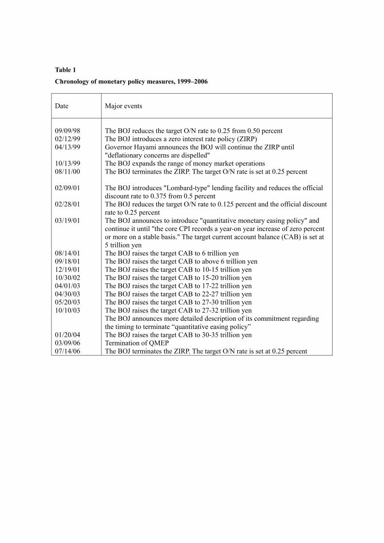
Table 1

Chronology of monetary policy measures, 1999–2006

Date

Major events

09/09/98 02/12/99 04/13/99 10/13/99 08/11/00 02/09/01 02/28/01 03/19/01 08/14/01 09/18/01 12/19/01 10/30/02 04/01/03 04/30/03 05/20/03 10/10/03 01/20/04 03/09/06 07/14/06

The BOJ reduces the target O/N rate to 0.25 from 0.50 percent The BOJ introduces a zero interest rate policy (ZIRP) Governor Hayami announces the BOJ will continue the ZIRP until "deflationary concerns are dispelled" The BOJ expands the range of money market operations The BOJ terminates the ZIRP. The target O/N rate is set at 0.25 percent The BOJ introduces "Lombard-type" lending facility and reduces the official discount rate to 0.375 from 0.5 percent The BOJ reduces the target O/N rate to 0.125 percent and the official discount rate to 0.25 percent The BOJ announces to introduce "quantitative monetary easing policy" and continue it until "the core CPI records a year-on year increase of zero percent or more on a stable basis." The target current account balance (CAB) is set at 5 trillion yen The BOJ raises the target CAB to 6 trillion yen The BOJ raises the target CAB to above 6 trillion yen The BOJ raises the target CAB to 10-15 trillion yen The BOJ raises the target CAB to 15-20 trillion yen The BOJ raises the target CAB to 17-22 trillion yen The BOJ raises the target CAB to 22-27 trillion yen The BOJ raises the target CAB to 27-30 trillion yen The BOJ raises the target CAB to 27-32 trillion yen The BOJ announces more detailed description of its commitment regarding the timing to terminate “quantitative easing policy” The BOJ raises the target CAB to 30-35 trillion yen Termination of QMEP The BOJ terminates the ZIRP. The target O/N rate is set at 0.25 percent

Table 2

The correlation between interventions and changes in current account balances

ttt uIR ++=∆ −2βµ (1)

FULL 1992/1/1-2001/12/18 2001/12/19-2006/3/9

µ

-0.016

(0.009)†

-0.006

(0.011)

-0.046

(0.020)*

β

0.188

(0.103)†

-0.004

(0.151)

0.389

(0.116)**

R2 Bar 0.052 0.016 0.162

OBS 3496 2461 1035

Notes: Heteroskedasticity-and-autocorrelation-consistent (HAC) standard errors are given in

parentheses.

†Statistically significant at the 10-percent level.

*Statistically significant at the 5-percent level.

**Statistically significant at the 1-percent level.

β=0: Sterilization is complete.

0<β<1: Sterilization is Not Complete.

β=1, Interventions are Unsterilized.

Table 3

Estimation of the policy response function (1)

tttt uIRR +++= −− 21 βρµ (2)

ttttt uIRRR ++++= −−− 2*

1*

1 βρρµ (3)

Eq(2)

2001/12/20-2006/3/9

Eq(3)

2001/12/19-2006/3/9

µ

2.796

(0.411)**

10.226

(0.966)**

ρ

0.819

(0.028)**

0.646

(0.033)**

ρ*

-0.012

(0.007)†

β

0.405

(0.106)**

0.460

(0.091)**

R2 Bar 0.990 0.832

OBS 1034 690

Notes: Heteroskedasticity-and-autocorrelation-consistent (HAC) standard errors are given in

parentheses.

†Statistically significant at the 10-percent level.

*Statistically significant at the 5-percent level.

**Statistically significant at the 1-percent level.

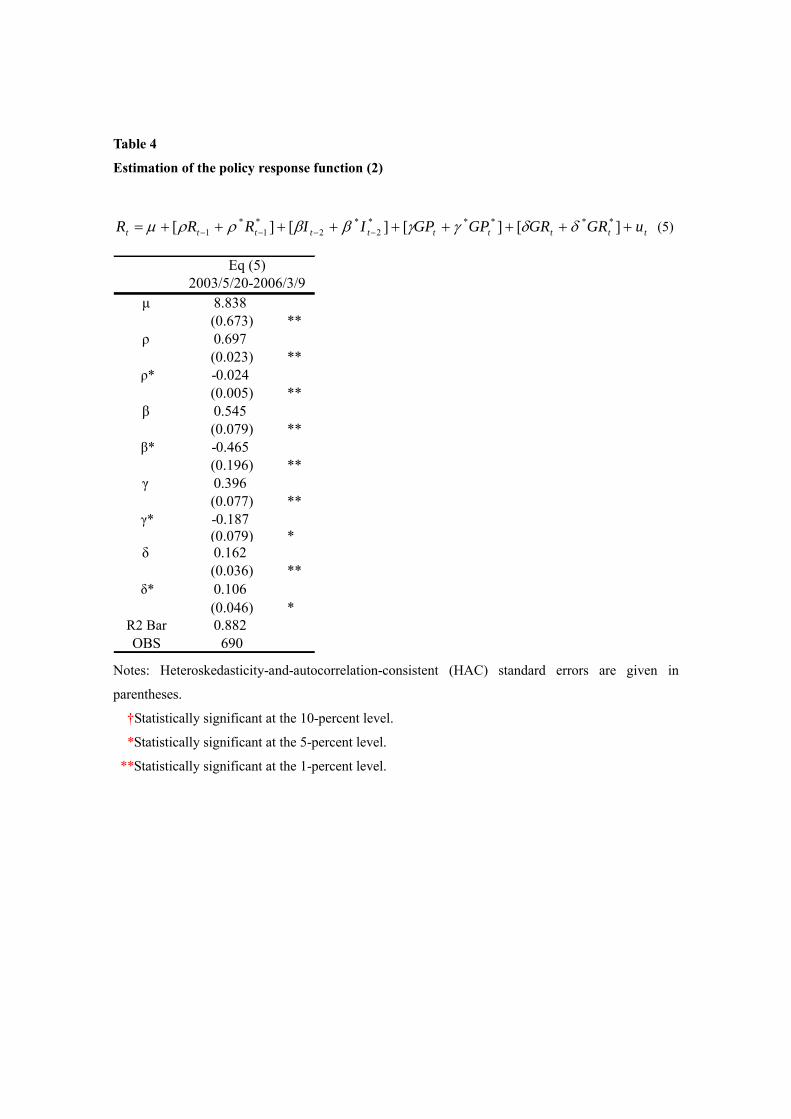
Table 4

Estimation of the policy response function (2)

tttttttttt uGRGRGPGPIIRRR +++++++++= −−−− ][][][][ *****2

*2

*1

*1 δδγγββρρµ (5)

µ 8.838(0.673) **

ρ 0.697(0.023) **

ρ* -0.024(0.005) **

β 0.545(0.079) **

β* -0.465(0.196) **

γ 0.396(0.077) **

γ* -0.187(0.079) *

δ 0.162(0.036) **

δ* 0.106(0.046) *

R2 Bar 0.882OBS 690

2003/5/20-2006/3/9Eq (5)

Notes: Heteroskedasticity-and-autocorrelation-consistent (HAC) standard errors are given in

parentheses.

†Statistically significant at the 10-percent level.

*Statistically significant at the 5-percent level.

**Statistically significant at the 1-percent level.