the Gordano Valley, North Somerset. PhD, University of the West...

Bridle, A. (2012) The mid-to-late pleistocene palaeoenvironments of

the Gordano Valley, North Somerset. PhD, University of the Westof England.

We recommend you cite the published version.The publisher’s URL is http://eprints.uwe.ac.uk/18104/

Refereed: No

(no note)

Disclaimer

UWE has obtained warranties from all depositors as to their title in the materialdeposited and as to their right to deposit such material.

UWE makes no representation or warranties of commercial utility, title, or fit-ness for a particular purpose or any other warranty, express or implied in respectof any material deposited.

UWE makes no representation that the use of the materials will not infringeany patent, copyright, trademark or other property or proprietary rights.

UWE accepts no liability for any infringement of intellectual property rightsin any material deposited but will remove such material from public view pend-ing investigation in the event of an allegation of any such infringement.

PLEASE SCROLL DOWN FOR TEXT.

http://eprints.uwe.ac.uk/18104/

209

Chapter 7 Characterisation of the Pleistocene minerogenic sediments of the Gordano

Valley

7.1 Introduction

This chapter addresses the third objective: to characterise the Pleistocene sediments

and interpret their depositional environments. This is achieved through the techniques

discussed in Chapter 4 (section 4.12) and both depositional and post-depositional

environments are interpreted. An assessment of particle size summary statistics is followed

by bivariate plots of particle size parameters, segment analysis, bivariate plots of gravel

clast shape and roundness data and gravel clast shape histograms. This information is then

combined with lithological evidence and palaeontological evidence (Chapter 6, sections 6.4

and 6.9) to infer a depositional history of the sediments. Stratigraphical (Chapter 6, section

6.2) and geochemical (section 6.7) evidence is then interpreted to infer post-depositional

environments. Finally, the geochronological evidence is discussed and interpreted.

7.2 Characterisation of sedimentary attributes to determine the Pleistocene

depositional environments

A preliminary assessment of depositional environments is possible from

examination of the particle size data presented in section 6.3, indicating the likelihood or

otherwise of some depositional environments; these are summarised in Table 7.1.

210

Table 7.1: Preliminary assessment of depositional environments from particle size data (source: Reineck &

Singh 1973)

Depositional

environment

Units Basis

Not aeolian GV3, GV4, GV5, GV6, GV9, GV10, GV11, PG7, PGA1,

PGA2, PGA3, PGA14, CGA3, CGA4, CGA5, CGA6, CGA7,

CGA12, CGA13, CGA14, CGB1, CGB2, CGB3, CGB7,

CGB9, CGB13,

NR2, NR3, NR4, NR5, NR6, NR7, NR9, NR13, NR14, NR15,

NR16, NR21, NR24, CM2, CM3, CM4, CM8, TG2, TG3,

TG8, TG9, TG12, TG13, TG14

Particle size

PGA13, PGA15, PGA16, PGA17, CGB5, NR1, NR10, NR11 Skewness

Not beach GV2, GV3, GV4, GV5, GV6, GV9, GV10, all units of core PG,

PGA1 to PGA14, all units of core CGB, all units of core CM

Very poor sorting

(σ 2-4)

All units of core CGA except CGA14 Very poor sorting

(σ 2-4) and skewness of

<1

All units of cores NR and TG Extremely poor sorting

(σ 1.3 - >4.0)

Not dune GV7, all units of core PG, PGA4, PGA6, PGA7, PGA8, PGA9,

PGA10, PGA11, PGA12, CGA1, CGA2, CGA8, CGA9,

CGA10, CGA11

Very poor sorting

(σ 2-4)

All units of core NR, all units of core TG Extremely poor sorting

(σ 1.3 - >4.0)

Fluvial GV11, CGA4, CGB2, NR3, NR4, NR5, NR6, NR14, NR15,

NR16, CM3, TG9, TG13

Bimodal particle size

distribution and positive

skewness

CGA14 Moderate sorting and

positive skewness

7.2.1 Bivariate plots of particle size parameters

Bivariance of particle size moments skewness against kurtosis (Figure 7.1) was

used to differentiate river, beach and aeolian/settling depositional characteristics. Aeolian

or settling deposition is indicated for fifty six units including a large number of gravel

units, such as CGB7, CGB13, NR16 and TG13; this probably reflects the depositional

environment of the gravel matrix.

211

0

0.5

1

1.5

2

2.5

3

3.5

-1 -0.8 -0.6 -0.4 -0.2 0 0.2 0.4

Skewness

Kurt

osis

River

Beach

Aeolian/settling

PG

0

5

10

15

20

25

30

-1.5 -1 -0.5 0 0.5 1 1.5 2 2.5 3 3.5 4 4.5 5

Skewness

Ku

rto

sis

Aeolian/settlingRiver

Beach

CGA

0

2

4

6

8

10

12

14

-1.0 -0.5 0.0 0.5 1.0 1.5 2.0 2.5 3.0 3.5

Skewness

Ku

rto

sis

sAeolian/settling

River

GV

0

2

4

6

8

10

12

-2 -1.5 -1 -0.5 0 0.5 1 1.5 2 2.5

Skewness

Ku

rto

sis

Aeolian/settling

River

Beach

PGA

0

0.5

1

1.5

2

2.5

3

3.5

4

-1 -0.5 0 0.5 1 1.5

Skewness

Ku

rto

sis

Aeolian/settling

River

BeachCGB

0

1

2

3

4

5

6

7

8

-1.5 -1 -0.5 0 0.5 1 1.5 2 2.5

Skewness

Ku

rto

sis

River

Beach

Aeolian/settling

NR

0

1

2

3

4

5

6

7

8

9

-2.5 -2 -1.5 -1 -0.5 0 0.5 1 1.5

Skewness

Ku

rto

sis

Aeolian/settling

BeachRiver

CM

0

2

4

6

8

10

12

-3 -2 -1 0 1 2 3

Skewness

Ku

rto

sis

Aeolian/settling

Beach

River

TG

Figure 7.1: Bivariate plots of sediment skewness against kurtosis (adapted from Tanner 1991). GV: GV1 plots

as a beach deposit. PG: PG7 plots as an aeolian/settling deposit; PG1 plots as a beach deposit. PGA: Eight

units plot as aeolian/settling deposits; PGA6 and PGA12 plot as beach deposits. CGA: Six units plot as

aeolian/settling deposits; five units plot as beach deposits. All other units in GV, PG, PGA and CGA plot as

river deposits. CGB: Four units plot as beach deposits (two plots coincide on the diagram). NR: Four units

plot as river deposits, four more units plot as beach deposits, NR19 and NR24 plot on the boundary between

river and aeolian deposition. CM: Three units plot as beach deposits. TG: Three units plot as river deposits,

seven units plot as beach deposits. All other units in CGB, NR, CM and TG plot as aeolian or settling

deposits; two plots coincide on the diagram for CGB

212

Fluvial deposition is indicated for thirty one units; two units (NR19 and NR24) plot

on the boundary between river and aeolian deposition. Beach deposition is indicated for

twenty six units. The depositional characteristics indicated are summarised in Table 7.2.

Table 7.2: Summary of depositional environments indicated by bivariance of particle size moments skewness

against kurtosis

Depositional

environment

Units

Aeolian/settling GV3, GV4, GV5, GV11, PG7, PGA1, PGA2, PGA3, PGA4, PGA8, PGA15, PGA16,

PGA17, CGA3, CGA4, CGA5, CGA6, CGA14, CGB1, CGB2, CGB3, CGB4, CGB5,

CGB6, CGB7 (CGB4 and CGB7 coincide on the diagram), CGB9, CGB13, NR1, NR2,

NR4, NR5, NR6, NR7, NR9, NR10, NR11, NR12, NR13, NR14, NR15, NR16, NR21,

NR26, TG2, TG3, TG4, TG5, TG8, TG9, TG12, TG13, TG14, TG17, TG19, TG21.

Fluvial GV1, GV6, GV7, GV8, GV9, PG2, PG3, PG4, PG5, PG6, PG8, PGA5, PGA10, PGA11,

PGA13, CGA2, CGA7, CGA8, NR17, NR18, NR20, NR22, CM1, CM5, CM6, CM7,

CM9, TG1, TG6, TG10, TG15

Beach GV1, PG1, PGA6, PGA12, CGA1, CGA9, CGA11, CGA12, CGA13, CGB8, CGB10,

CGB11, CGB12 (CGB11 and CGB12 coincide on the diagram), NR3, NR8, NR23,

NR25, CM10, CM12, CM13, TG7, TG11, TG16, TG18, TG20, TG22

Bivariance of mean particle size against sorting for the >4 φ fraction of sediments

was used to differentiate between river and closed basin/settling depositional environments.

Figure 7.2 shows that all Gordano Valley sediments demonstrate river or closed

basin/settling depositional characteristics; plots cluster close to the river environmental

envelope, with most units plotting in the closed basin/settling environmental envelope. This

indicates that for most units deposition was in a closed basin-type environment with a

nearby river. CGA14 plots furthest from the river envelope, suggesting a diminished fluvial

influence in its depositional environment. Fluvial deposition is indicated for units GV1,

GV2, GV5, GV8, NR11, NR16, NR19, NR23 and TG1, which plot within the river

depositional envelope.

213

1.00

1.05

1.10

1.15

5678910

Mean particle size (phi)

So

rtin

g (

ph

i)

RiverClosed

basin/settling

PGA

1.00

1.05

1.10

1.15

5678910


So

rtin

g (

ph

i)

RiverClosed

basin/

settling

PG

1.00

1.05

1.10

1.15

1.20

5678910


Sort

ing (

phi)

River Closed

basin/settling

GV

1.00

1.05

1.10

1.15

1.20

5678910


So

rtin

g (

ph

i)

RiverClosed

basin/

settling

CGA

1.00

1.05

1.10

1.15

1.20

1.25

5678910


So

rtin

g (

ph

i)

RiverClosed

basin/

settling

NR

1.00

1.05

1.10

1.15

1.20

5678910


So

rtin

g (

ph

i)

Closed

basin/

settling

River

CGB

1.00

1.05

1.10

1.15

1.20

5678910


So

rtin

g (

ph

i)

RiverClosed basin/

settling

CM

1.00

1.05

1.10

1.15

1.20

1.25

1.30

5678910


So

rtin

g (

ph

i)

RiverClosed basin/

settling

TG

Figure 7.2: Bivariate plots of mean particle size against sorting for the >4 φ fraction (adapted from Lario et al.

2002). The plots cluster around the closed basin/settling depositional envelope, close to the river envelope;

units, GV1, GV2, GV5, GV8, NR11, NR16, NR19, NR23 and TG11 plot within the river depositional

envelope

Bivariance of median particle size against skewness and of median particle size

against sorting was used to differentiate between river, wave and quiet water depositional

characteristics. The plots of median particle size against skewness (Figure 7.3) show that

214

thirty two units plot in the river depositional envelope, sixteen units plot in the wave

environmental envelope, NR23 and CM9 plot in the overlap between the river and wave

envelopes and GV6 plots close to the wave envelope. CGB4, CGB5 NR10, NR11 and

NR26, plot in the quiet water, slow deposition envelope and CM11 plots on the boundary

for quiet water, slow deposition. Just over half the units plot outside any of the recognised

environmental envelopes; CGA4 plots on its own on the left of the CGA diagram and

CGA14 plots on its own at the top of the diagram.

-1

0

1

0 2 4 6

Median particle size (phi)S

ke

wn

ess (

ph

i)

River

Waves

Quiet water

slow deposition

PG

-2

-1

0

1

2

3

4

-6 -4 -2 0 2 4 6 8

Median particle size (phi)

Ske

wn

ess (

ph

i)

River

Waves

Quiet

water

slow

deposition

-2

-1

0

1

2

3

-1 0 1 2 3 4 5 6 7


Ske

wn

ess (

ph

i)

River

Waves

Quiet

water

slow

deposition

GV

PGA

-2

-1

0

1

2

3

4

5

-4 -2 0 2 4 6


Ske

wn

ess (

ph

i)

Waves

Quiet water

slow deposition

River

CGA

Figure 7.3: Bivariate plots of sediment median particle size against skewness (adapted from Stewart 1958).

GV: GV9 and GV10 plot in the river environmental envelope. PG: Three units plot in the river environmental

envelope; PG1 plots in the waves envelope. PGA: Three units plot in the river environmental envelope; two

units plot in the waves environmental envelope. CGA: Three units plot in the river environmental envelope;

six units plot in the waves envelope; CGA4 plots on its own on the left of the diagram; CGA14 plots on its

own at the top of the diagram. All other units plot outside the environmental envelopes

215

-3

-2

-1

0

1

2

3

-6 -4 -2 0 2 4 6 8


Ske

wn

ess (

ph

i)

RiverWaves

Quiet

water

slow

deposition

TG

-2.5

-2

-1.5

-1

-0.5

0

0.5

1

1.5

-4 -2 0 2 4 6 8

Median particle s ize (phi)

Ske

wn

ess (

ph

i)

RiverWaves

Quiet water

slow

deposition

CM

-1

0

1

2

3

-6 -4 -2 0 2 4 6


Ske

wn

ess (

ph

i)

River

Waves

Quiet

water

slow

deposition

NR

-1

-0.5

0

0.5

1

1.5

-4 -2 0 2 4


Ske

wn

ess (

ph

i)

River

Waves

Quiet water

slow

deposition

CGB

Figure 7.3 (continued): Bivariate plots of sediment median particle size against skewness. CGB: Three units

plot in the river environmental envelope; four units plot in the waves envelope; CGB4 and CGB5 plot in the

quiet water envelope. NR: Nine units plot in the river environmental envelope; four units plot in the waves

environmental envelope; NR23 plots in the overlap between the river and waves envelopes; three units plot in

the quiet water, slow deposition envelope. CM: Three units plot in the river environmental envelope; CM10

and CM12 plot in the waves envelope; CM9 plots in the overlap between the two environments. TG: TG8 and

TG12 plot in the river environmental envelope; TG20 plots in the waves environmental envelope. All other

units plot outside the environmental envelopes

However, plots of median particle size against sorting (Figure 7.4) show that no

units plot in the waves envelope, and only CGA14 plots in the rivers envelope, whilst thirty

four units plot in the quiet water, slow deposition envelope, with GV6, GV9 and GV10

plotting close to this envelope. Most units again plot outside the environmental envelopes

with CGA4 again plotting on its own on the left of the diagram.

The depositional characteristics indicated by bivariance of median particle size

against skewness and of median particle size against sorting are summarised in Table 7.3.

216

0

1

2

3

4

-2 0 2 4 6 8


So

rtin

g (

ph

i)

Quiet water

slow

deposition

River

Waves

PGA

0

1

2

3

4

5

0 2 4 6


So

rtin

g (

ph

i)

Quiet water

slow

deposition

River

Waves

PG

0

1

2

3

4

5

6

-6 -4 -2 0 2 4 6 8


So

rtin

g (

ph

i)

Quiet water

slow

deposition

RiverWaves

GV

0

1

2

3

4

-4 -2 0 2 4 6


Sort

ing (

phi)

Quiet water

slow

deposition

RiverWaves

CGA

Sort

ing

(phi)

0

1

2

3

4

5

-6 -4 -2 0 2 4 6


So

rtin

g (

ph

i)

Quiet

water

slow

deposition

River

Waves

NR

0

1

2

3

4

5

6

-6 -4 -2 0 2 4 6 8


So

rtin

g (

ph

i)

Quiet water

slow

deposition

River

Waves

TG

0

1

2

3

4

5

-4 -2 0 2 4

Median particle s ize (phi)

So

rtin

g (

ph

i)

River

Waves

Quiet

water

slow

deposition

CGB

0

1

2

3

4

5

-4 -2 0 2 4 6


So

rtin

g (

ph

i)

Quiet

water

slow

deposition

RiverWaves

CM

Figure 7.4: Bivariate plots of sediment median particle size against sorting (adapted from Stewart 1958).

GV: Four units plot in the quiet water, slow deposition environmental envelope. PG: Four units plot in the

quiet water, slow deposition environmental envelope. PGA: Six units plot in the quiet water, slow deposition

envelope. CGA: CGA14 plots in the river environmental envelope; five units plot in the quiet water slow,

deposition environmental envelope; CGA4 plots on its own on the left of the diagram, outside the

environmental envelopes. CGB: CGB11 plots in the quiet water, slow deposition environmental envelope.

NR: NR20 and NR22 plot in the quiet water, slow deposition envelope. CM: Five units plot in the quiet water,

slow deposition environmental envelope. TG: Seven units plot in the quiet water, slow deposition envelope.

All other units plot outside the environmental envelopes

217

Table 7.3: Summary of depositional environments indicated by bivariance of median particle size against

skewness and of median particle size against sorting

Indicator Depositional

environment

Units

Median particle

size against

skewness

River GV9, GV10, PG4, PG7, PG8, PGA1, PGA3, PGA14, CGA5,

CGA6, CGA13, CGB3, CGB9, CGB13, CGB8, CGB10, CGB11,

CGB12, NR3, NR5, NR7, NR8, NR12, NR13, NR19, NR21, NR24

CM2, CM4, CM8, TG8, TG12

Waves PG1, PGA7, PGA9, CGA1, CGA2, CGA3, CGA10, CGA11,

CGA12, NR17, NR18, NR22, NR25, CM10, CM12, TG20

Quiet water, slow

deposition

CGB4, CGB5, NR10, NR11, NR26

Median particle

size against

sorting

River CGA14

Quiet water, slow

deposition

GV1, GV2, GV7, GV8, PG2, PG3, PG5, PG6, PGA6, PGA9,

PGA10, PGA11, PGA12, PGA13, CGA2, CGA7, CGA8, CGA9,

CGA11, CGB11, NR20, NR22, CM1, CM5, CM6, CM7, CM13,

TG4, TG10, TG11, TG15, TG18, TG20, TG21

Bivariance of median particle size against the particle size of the coarsest one

percentile was used to differentiate between mudflow, river channel and braided stream

depositional characteristics. The pattern of plots shown in Figure 7.5 suggests water-lain

deposition for most units and indicates mudflow characteristics for twenty units, and

probably also PG5, PG6, CGA7 and NR22 which plot just outside the lower end of the

mudflow depositional envelope, indicating higher competence of the transporting agent

(Bull 1962). Braided stream deposition is indicated for twenty six units; the proximity of

CGA14 to the x = y line indicates its better sorting (Bull 1962) and although it falls outside

the known envelope for braided stream deposition, probably still represents deposition by

braided stream. PGA8, CGA3 and CGB6 could be either braided stream or river channel

deposits as they plot in the overlap between the two environments.

218

-6

-5

-4

-3

-2

-1

0

-5 -4 -3 -2 -1 0 1 2 3 4 5 6


Pa

rtic

le s

ize

of

coa

rse

st

on

e p

erc

en

tile

(ph

i)

PG

River

channel

Braided

stream

Mudflow

-7

-6

-5

-4

-3

-2

-1

0

1

2

3

-6 -5 -4 -3 -2 -1 0 1 2 3 4 5 6 7


Pa

rtic

le s

ize

of

coa

rse

st

on

e p

erc

en

tile

(ph

i)

GV

River

channel

Braided

stream

Mudflow

-6

-5

-4

-3

-2

-1

0

-5 -4 -3 -2 -1 0 1 2 3 4 5 6


Pa

rtic

le s

ize

of

coa

rse

st

on

e p

erc

en

tile

(ph

i)

CGA

River

channel

Braided

stream

Mudflow

-6

-5

-4

-3

-2

-1

0

1

-5 -4 -3 -2 -1 0 1 2 3 4 5 6 7


Pa

rtic

le s

ize

of

coa

rse

st

on

e p

erc

en

tile

(ph

i)

PGA

River

channel

Braided

stream

Mudflow

Pa

rtic

le s

ize

of

coa

rse

st

on

e p

erc

en

tile

(ph

i)

-7

-6

-5

-4

-3

-2

-1

0

1

2

3

4

-5 -4 -3 -2 -1 0 1 2 3 4 5 6 7


TG

River

channel

Braided

stream

Mudflow

-6

-5

-4

-3

-2

-1

0

-5 -4 -3 -2 -1 0 1 2 3 4 5 6 7


Pa

rtic

le s

ize

of

coa

rse

st

on

e p

erc

en

tile

(ph

i)

CM

River

channel

Braided

stream

Mudflow

Pa

rtic

le s

ize

of

coa

rse

st

on

e p

erc

en

tile

(ph

i)

-7

-6

-5

-4

-3

-2

-1

0

1

-5 -4 -3 -2 -1 0 1 2 3 4 5 6


NR

-7

-6

-5

-4

-3

-2

-1

0

1

-5 -4 -3 -2 -1 0 1 2 3 4


Pa

rtic

le s

ize

of

coa

rse

st

on

e p

erc

en

tile

(ph

i)

CGB

River

channel

Braided

stream

River

channel

Braided

stream

Mudflow

Figure 7.5: Bivariate plots of median particle size against the particle size of the coarsest one percentile

(adapted from Bull 1962). GV: Three units plot as mudflow deposits, GV7 plots as a braided stream deposit

and four units plot outside the environmental envelopes. PG: PG2 and PG3 plot as mudflow deposits; PG5

and PG6 are also probably mudflow deposits as they plot marginally to the mudflow envelope. PGA: Five

units plot as braided stream deposits, PGA8 plots in the overlap between braided stream and river channel

deposition, five units plot as mudflow deposits, PGA9 plots outside the environmental envelopes,

intermediate between the mudflow and river channel envelopes. CGA: CGA9 plots as a mudflow deposit;

CGA7 plots marginally to the mudflow envelope and is also probably a mudflow deposit; CGA1 plots as a

braided stream deposit; CGA3 plots in the overlap between braided stream and river channel deposit; three

units plot as intermediate between mudflow and river channel environments; CGA4, CGA7 & CGA14 plot

outside the environmental envelopes. CGB: CGB4 and CGB5 plot as a braided stream deposits; CGB6 plots

219

in the overlap between braided stream and river channel deposits; CGB11 and CGB12 plot outside the

environmental envelopes. NR: NR20 plots as a mudflow deposit, four units plot as braided stream deposits,

five units plot outside the environmental envelopes. CM: CM11 and CM13 plot as a braided stream deposits,

four units plot as mudflow deposits, CM12 plots just outside the environmental envelope for river channel

deposition. TG: Four units plot as mudflows, three units plot beyond the end of the river channel envelope;

eleven units plot as braided stream deposits; four units plot as river channel deposits

River channel characteristics are indicated for fifty one units; this probably extends

to GV3, GV4, GV5 and GV11, CGA4, NR2, NR9, NR15 and NR16, TG2, TG3, and TG14

which plot outside the left-hand side of the river channel envelope, indicating higher

competence of the transporting agent (Bull 1962), suggesting deposition from a turbulent

river. CM12 plots just outside the opposite end of the environmental envelope for river

channel deposition, suggesting deposition from a quieter stream. PGA9, CGA2, CGA8 and

CGA11 plot intermediate between the mudflow and river channel envelopes, TG10 plots

intermediate between mudflow and braided stream deposition and CGB11 and CGB12 plot

between the environmental envelopes for mudflow, braided stream and river channel

deposition. Table 7.4 provides as summary of the characteristics indicated.

7.2.2 Segment analysis

Segment analysis (section 4.12.1) of particle size data was used to separate

sediments into sandy river, dune or river silts/closed basin groups. These are shown in

Figure 7.6. The depositional environments indicated are summarised in Table 7.5.

The sediments of core GV separate into four groups: a sandy river group (GV10,

probably also GV4 and GV5), a river silts and clays or closed basin group (GV7, probably

also GV6 and GV9), which has some overlap with a dune group (GV6). The fourth group

falls outside the parameters of the segments and is divided into two sub-groups: one which

plots in the coarse tail close to the sandy river envelope, comprises gravel units and

probably represents a fluvial gravel population (GV3 and GV11) and another which plots

closest to the river silts and dune segments (GV1, GV2 and GV8).

220

Table 7.4: Summary of depositional environments indicated by bivariance of median particle size against the

particle size of the coarsest one percentile

Depositional

environment

Units

Mudflow GV1, GV2, GV8

PG2, PG3, probably PG5, PG6

PGA5, PGA10, PGA11, PGA12, PGA13

CGA9, probably CGA7

NR20, probably NR22

CM1, CM5, CM6, CM7

TG1, TG10, TG11, TG15

River channel GV6, GV9, GV10, probably GV3, GV4, GV5, GV11

PG1, PG4, PG7, PG8


CGA5, CGA6, CGA10, CGA12, CGA13, probably CGA4

CGB1, CGB2, CGB3, CGB7, CGB8, CGB9, CGB 10, CGB13

NR3, NR4, NR5, NR6, NR7, NR8, NR12, NR13, NR14, NR17, NR18, NR19, NR21,

NR23, NR24, NR25, probably NR2, NR9, NR15 & NR16

CM2, CM3, CM4, CM8, CM9, CM10

TG8, TG9, TG12, TG13 probably TG2, TG3, TG14

Braided stream GV7


CGA1, probably CGA14

CGB4, CGB5

NR1, NR10, NR11, NR26

CM11, CM13

TG4, TG5, TG6, TG7, TG16, TG17, TG18, TG19, TG20, TG21, TG22

The sediments of core PG separate into three groups: a sandy river group (PG7,

probably also PG8), a dune group (PG1 and PG4) and a group which falls outside the

segments, but which plots closest to the river silts segment (PG2, PG3, PG5 and PG6).

Core PGA sediments separate into five groups: a ‘No tail’ group, representing a

beach environment (PGA15, PGA16 and PGA17), a sandy river group (PGA1, PGA2,

PGA14), a river silts and clays or closed basin group (PGA4, PGA5, PGA6 and PGA10), a

dune group (PGA7), and a group that plots outside the parameters of the segments (PGA9,

PGA11, PGA12 and PGA13). PGA3 which plots marginally to the boundary of the sandy

221

river segment and PGA8 which plots on the boundary between sandy river and dune

environments probably form part of the sandy river group.

No tail

Coarse tailFine tail

Dune

River silts &

clays or

closed basin

Sandy river

TG13

TG19

TG4

TG7

TG16

TG5

TG6

TG14TG15

TG1

TG11

TG18

TG10

TG9

TG12TG20

TG17

TG8

TG2TG3

TG21

TG22

TG

No tail


Dune

River silts &

clays or

closed basin

Sandy

river

CGB10

CGB9CGB8

CGB4

CGB2

CGB3

CGB11

CGB7

CGB1

CGB5

CGB6

CGB12

CGB13

CGB

No tail


River silts &

clays or

closed

basin

CM1

Dune

Sandy

river

CM6

CM10CM11

CM12

CM5

CM4

CM2

CM9 CM8

CM7

CM13

CM3

CM

NR23

No tail


River silts &

clays or

closed basin

Dune

Sandy

river

NR12

NR10 NR1

NR11

NR18

NR25

NR26

NR20

NR22

NR17

NR19

NR24

NR21

NR3

NR13

NR8

NR14

NR9

NR2

NR16

NR5

NR7

NR4

NR6

NR15

NR

No tail


River silts &

clays or

closed basin

Sandy

river

Dune

CGA1

CGA2, CGA3,

CGA10 & CGA12

CGA4

CGA5

CGA6

CGA7, CGA8

& CGA11

CGA9

CGA13

CGA14

CGA

No tail


River silts &

clays or

closed basin

Dune

Sandy river

PGA1

PGA2

PGA3

PGA4

PGA5

PGA6

PGA7

PGA10 PGA11PGA12

PGA13

PGA16

PGA9

PGA14

PGA17

PGA8

PGA15

PGA

No tail


Dune

River silts &

clays or closed

basin

Sandy

river

PG6

PG5

PG3

PG2

PG8

PG4 PG7

PG1

PGNo tails


Sandy

river

Dune

River silts &

clays or closed

basin

GV1

GV2GV3

GV4

GV5

GV6

GV7

GV8

GV9

GV10

GV11

GV

Figure 7.6: Segment analysis of the Gordano Valley sediments (adapted from Tanner 1991). GV: GV6 plots

as either a dune or river silts & clays or closed basin deposit; seven units plot outside the segment parameters.

PG: PG8 plots between dune and sandy river deposits, slightly closer to the sandy river segment; four units

plot outside the segment parameters. PGA: PGA8 plots on the boundary between sandy river and dune

environments and PGA3 plots marginally to the boundary of the sandy river segment. CGA: CGA1 plots as

either dune or river silts & clays or closed basin deposits; three units plot outside the segment parameters.

CGB: CGB8, CGB9 and CGB10 plot as either dune or river silts & clays or closed basin deposits; CGB13

plots marginally outside the sandy river segment. NR: Five units plot in the overlap between dune deposits

and those of river silt and clay or closed basin deposits. CM: CM3 plots as either dune or river silts & clays or

closed basin deposits; three units plot outside the segment parameters. TG: TG20 plots in the overlap between

dune deposits and those of river silt and clay or closed basin deposits

Core CGA sediments separate into five groups: a sandy beach (no tail) group

(CGA14), a sandy river group (CGA4, CGA5, CGA6 and CGA13), a river silts and clays

222

or closed basin group (CGA9 and possibly CGA1), which has some overlap with the dune

group (CGA2, CGA3, CGA10 CGA12 and possibly CGA1), and a group which falls

outside the parameters of the segments (CGA7, CGA8 and CGA11).

The sediments of core CGB separate into four groups: a sandy river group (CGB1,

CGB5, CGB6, CGB7, CGB11 and CGB12), a river silts and clays or closed basin group

(CGB3, probably also CGB8, CGB9 and CGB10), which has some overlap with the dune

group (CGB2 and CGB4) and CGB13 which plots outside the parameters of the segments,

but probably constitutes part of the sandy river group.

The sediments of core NR separate into four groups: a dune group (NR18 and

NR25), a river silts and clays or closed basin group (NR1, NR10, NR11, NR12 and NR26),

which overlaps the dune segment so could have been deposited in either environment; a

group that plots outside the parameters of the segments (NR17, NR19, NR20, NR22 and

NR24); the remaining units plot in the sandy river group.

Core CM sediments separate into five groups: a sandy river group (CM6, CM10,

CM11 and CM12), a river silts and clays or closed basin group (CM1 and CM13), which

has some overlap with the dune or river silts group (CM3), the dune group (CM2, CM4 and

CM5), and CM7, CM8 and CM9 which plot outside the parameters of the segments.

Table 7.5: Summary of depositional environments indicated by segment analysis.

Units not shown plot outside the environmental parameters

Depositional environment Units

Sandy river GV10, possibly GV4 & GV5, PG7, possibly PG8, PGA1, PGA2,

PGA14, probably PGA3 & PGA8, CGA4, CGA5, CGA, CGA13,

CGB1, CGB5, CGB6, CGB7, CGB11, CGB12, NR2, NR3, NR4, NR5,

NR6, NR7, NR8, NR9, NR13, NR14, NR15, NR16, NR21, NR23,

CM6, CM10, CM11, CM12, TG8, TG9, TG12

River silts & clays or closed basin GV7, possibly GV6 & GV9, PGA4, PGA5, PGA6, PGA10, CGA9,

possibly CGA1, CGB3, probably CGB8, CGB9 & CGB10, NR1,

NR10, NR11, NR12, NR26, CM1, CM13, possibly CM3, TG1, TG4,

TG5, TG6, TG7, TG10, TG11, TG16, TG17, TG18, TG19, TG21,

TG22

Dune PG1, PG4, PGA7, CGA2, CGA3, CGA10, CGA12, possibly CGA1,

CGB2, CGB4, NR18, NR25, CM2, CM4, CM5

Beach PGA15, PGA16, PGA17, CGA14

223

The sediments of core TG separate into four groups: a sandy river group (TG8, TG9

and TG12); TG20 plots in the overlap between the river silts and clays or closed basin

segment and the dune segments; TG2, TG3, TG13, TG14 and TG15 plot outside the

parameters of the segments. The remainder and largest group of units plot in the river silts

and clays or closed basin group.

7.3 Bivariate plots of gravel clast morphology

Bivariance of limestone gravel clast morphology parameters (mean sphericity

against mean OPI) was used to differentiate river and beach depositional characteristics and

bivariance of clast morphology against roundness (C40 against RA) was used to determine

whether any of the gravels had glacial characteristics.

7.3.1 Bivariance of gravel clast sphericity and OPI

The bivariate plot of mean clast sphericity against mean OPI (Figure 7.7) indicates

beach depositional characteristics for most of the Gordano Valley gravels; fluvial

characteristics are indicated for PG7, CGB1, CGB7, NR9, NR13, NR21 and TG3.

-3.5

-3.0

-2.5

-2.0

-1.5

-1.0

-0.5

0.0

0.5

1.0

0.60 0.61 0.62 0.63 0.64 0.65 0.66 0.67 0.68 0.69 0.70

Mean sphericity

Fluvial

Fluvial

Beach

Me

an

OP

I

GV11

CM8

NR9

TG3

PG7

TG13

NR13CGB7CGB1

NR16

PGA14

NR2

GV3

CGA4

CM4

NR7

NR21

TG9

CGB13

NR6

CM3

Figure 7.7: Bivariate plot of mean sphericity against mean OPI (adapted from Dobkins & Folk 1970) for

Gordano Valley gravels. The plots for CGB1 and NR21 coincide. The dotted red line represents the boundary

between beach and fluvial environments

224

7.3.2 Bivariance of gravel clast morphology and roundness

The bivariate plot of clast morphology against roundness (Figure 7.8) indicates

moraine characteristics for most of the Gordano Valley gravels, with a number of gravels

also plotting marginally to the moraine envelope. NR21 plots close to the envelope for

deposits of known scree origin.

0

20

40

60

80

100

0 20 40 60 80 100

% C40

Gordano Valley gravels Till Scree Moraine Supraglacial

Ro

und

ne

ss %

RA

NR9

TG3

PGA14

NR21

CM8NR2

GV3

GV11

CM4

CGB1

TG9

CGB13PG7

NR7

CGA4/NR13CGB7

CM3

NR6

TG13NR16

Figure 7.8: Bivariate plot of %C40 against %RA (adapted from Evans & Benn 2004 with additional data from

Benn & Ballantyne 1993, 1994). Most gravels plot within the parameters for known moraine deposits; CGA4

and NR13 coincide on the plot. CGB1, NR2, NR9 and CM4 plot marginally to deposits of known moraine

origin and NR21 plots close to deposits of known scree origin

7.3.3 Gravel clast morphology histograms

Frequency histograms of the values of gravel clast (a-b)/(a-c) measurements (Sneed

& Folk 1958) are shown in Figure 7.9. Polymodal distributions for most Gordano Valley

gravels indicate the gravels comprise multiple components. However, CM4 and CM8 have

bimodal distributions, suggesting these gravels comprise just two components, whilst GV3

has an almost Gaussian distribution, indicating this gravel does not comprise multiple

components.

225

GV3

0

5

10

15

20

0-0.1

0.1-0.2

0.2-0.3

0.3-0.4

0.4-0.5

0.5-0.6

0.6-0.7

0.7-0.8

0.8-0.9

0.9-1

a-b/a-c

%

GV11

0

5

10

15

20

25

0-0.1

0.1-0.2

0.2-0.3

0.3-0.4

0.4-0.5

0.5-0.6

0.6-0.7

0.7-0.8

0.8-0.9

0.9-1

a-b/a-c

%

PG7

0

5

10

15

20

0-0.1

0.1-0.2

0.2-0.3

0.3-0.4

0.4-0.5

0.5-0.6

0.6-0.7

0.7-0.8

0.8-0.9

0.9-1

a-b/a-c

%

PGA14

0

5

10

15

20

0-0.1

0.1-0.2

0.2-0.3

0.3-0.4

0.4-0.5

0.5-0.6

0.6-0.7

0.7-0.8

0.8-.9

0.9-1

a-b/a-c

%

CGA4

0

5

10

15

20

0-0.1

0.1-0.2

0.2-0.3

0.3-0.4

0.4-0.5

0.5-0.6

0.6-0.7

0.7-0.8

0.8-0.9

0.9-1

a-b/a-c

%

CGB1

0

5

10

15

20

0-0.1

0.1-0.2

0.2-0.3

0.3-0.4

0.4-0.5

0.5-0.6

0.6-0.7

0.7-0.8

0.8-0.9

0.9-1

a-b/a-c

%

CGB7

0

5

10

15

20

25

0-0.1

0.1-0.2

0.2-0.3

0.3-0.4

0.4-0.5

0.5-0.6

0.6-0.7

0.7-0.8

0.8-0.9

0.9-1

a-b/a-c

%

CGB13

0

5

10

15

20

25

0-0.1

0.1-0.2

0.2-0.3

0.3-0.4

0.4-0.5

0.5-0.6

0.6-0.7

0.7-0.8

0.8-0.9

0.9-1

a-b/a-c

%

NR2

02468

10121416

0-0.1

0.1-0.2

0.2-0.3

0.3-0.4

0.4-0.5

0.5-0.6

0.6-0.7

0.7-0.8

0.8-0.9

0.9-1

a-b/a-c

%

NR6

0

5

10

15

20

0-0.1

0.1-0.2

0.2-0.3

0.3-0.4

0.4-0.5

0.5-0.6

0.6-0.7

0.7-0.8

0.8-0.9

0.9-1

a-b/a-c

%

Figure 7.9: Frequency histograms of the values of the (a-b)/(a-c) measurements for the Gordano Valley

gravels (adapted from Sneed & Folk 1958)

226

NR7

0

5

10

15

20

0-0.1

0.1-0.2

0.2-0.3

0.3-0.4

0.4-0.5

0.5-0.6

0.6-0.7

0.7-0.8

0.8-0.9

0.9-1

a-b/a-c

%

NR9

0

5

10

15

20

25

0-0.1

0.1-0.2

0.2-0.3

0.3-0.4

0.4-0.5

0.5-0.6

0.6-0.7

0.7-0.8

0.8-0.9

0.9-1

a-b/a-c

%

NR13

05

10152025

3035

0-0.1

0.1-0.2

0.2-0.3

0.3-0.4

0.4-0.5

0.5-0.6

0.6-0.7

0.7-0.8

0.8-0.9

0.9-1

a-b/a-c

%

NR16

0

5

10

15

20

25

0-0.1

0.1-0.2

0.2-0.3

0.3-0.4

0.4-0.5

0.5-0.6

0.6-0.7

0.7-0.8

0.8-0.9

0.9-1

a-b/a-c

%

NR21

0

5

10

15

20

0-0.1

0.1-0.2

0.2-0.3

0.3-0.4

0.4-0.5

0.5-0.6

0.6-0.7

0.7-0.8

0.8-0.9

0.9-1

a-b/a-c

%

CM3

0

5

10

15

20

25

0-0.1

0.1-0.2

0.2-0.3

0.3-0.4

0.4-0.5

0.5-0.6

0.6-0.7

0.7-0.8

0.8-0.9

0.9-1

a-b/a-c

%

CM4

0

5

10

15

20

25

0-0.1

0.1-0.2

0.2-0.3

0.3-0.4

0.4-0.5

0.5-0.6

0.6-0.7

0.7-0.8

0.8-0.9

0.9-1

a-b/a-c

%

CM8

0

5

10

15

20

0-0.1

0.1-0.2

0.2-0.3

0.3-0.4

0.4-0.5

0.5-0.6

0.6-0.7

0.7-0.8

0.8-0.9

0.9-1

a-b/a-c

%

TG3

0

5

10

15

20

0-0.1

0.1-0.2

0.2-0.3

0.3-0.4

0.4-0.5

0.5-0.6

0.6-0.7

0.7-0.8

0.8-0.9

0.9-1

a-b/a-c

%

TG9

02468

10121416

0-0.1

0.1-0.2

0.2-0.3

0.3-0.4

0.4-0.5

0.5-0.6

0.6-0.7

0.7-0.8

0.8-0.9

0.9-1

a-b/a-c

%

TG13

0

5

10

15

20

0-0.1

0.1-0.2

0.2-0.3

0.3-0.4

0.4-0.5

0.5-0.6

0.6-0.7

0.7-0.8

0.8-0.9

0.9-1

a-b/a-c

%

Figure 7.9 (continued): Frequency histograms of the values of the (a-b)/(a-c) measurements for the Gordano

Valley gravels (adapted from Sneed & Folk 1958)

227

7.4 Interpretation of sedimentary evidence of depositional environments

The sedimentary attributes inferred from the analyses presented above, together

with the results for clast lithological analysis presented in section 6.4, allow an

interpretation of the depositional characteristics to be made for each sedimentary unit.

Characteristics inferred from particle size attributes are assessed first, followed by those

from gravel clast morphology and roundness.

7.4.1 General sedimentary characteristics

Most units have bi- or multimodal particle size distributions, indicative of reworked

deposits (Weltje & Prins 2007); there are no unimodal particle size distributions in cores

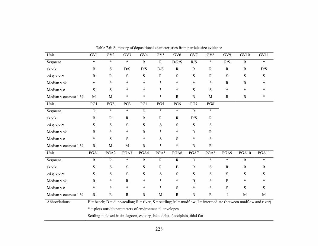
PG, CGB and CM and most units are very to extremely poorly sorted. Table 7.6 shows that

all units have some characteristics of settling deposition (indicative of closed basin

deposition: lake, lagoon, estuary, delta, floodplain or tidal flat for example, Tanner 1991),

which probably reflects the configuration of the valley. Fluvial characteristics are also

indicated for most units: only seven units show no characteristics of fluvial deposition.

Sixty seven units have some characteristics of aeolian deposition, twenty units have the

characteristics of deposition from mudflow and forty one units have some characteristics of

beach deposition. Sediment sorting indicates beach deposition is likely, therefore where

beach characteristics are indicated these are attributed to winnowing of fine material under

waning flow and sediments are interpreted as fluvial lag deposits.

Analysis of gravel attributes (Table 7.7) indicates that gravel units were deposited in

either fluvial or beach environments. Fluvial characteristics are indicated for eight gravels,

whilst high energy beach characteristics are indicated for two gravels (GV11 and CM8),

low energy beach characteristics are indicated for ten gravels and NR6 is shown to be both

a high and low energy beach; only NR16 is indeterminate, being either fluvial or beach

gravel. Fourteen gravel units (PG7, CGA4, all core CGB and CM gravels, four gravels in

core NR and two gravels in core TG) have characteristics of glacial (moraine) deposition

and NR21 has scree characteristics.

228

Table 7.6: Summary of depositional characteristics from particle size evidence

Unit GV1 GV2 GV3 GV4 GV5 GV6 GV7 GV8 GV9 GV10 GV11

Segment * * * R R D/R/S R/S * R/S R *

sk v k B S D/S D/S D/S R R R R R D/S

>4 φ x v σ R R S S R S S R S S S

Median v sk * * * * * * * * R R *

Median v σ S S * * * * S S * * *

Median v coarsest 1 % M M * * * R R M R R *

Unit PG1 PG2 PG3 PG4 PG5 PG6 PG7 PG8

Segment D * * D * * R *

sk v k B R R R R R D/S R

>4 φ x v σ S S S S S S S S

Median v sk B * * R * * R R

Median v σ * S S * S S * *

Median v coarsest 1 % R M M R * * R R

Unit PGA1 PGA2 PGA3 PGA4 PGA5 PGA6 PGA7 PGA8 PGA9 PGA10 PGA11

Segment R R * R R R D * * R *

sk v k S S S S R B R S R R R

>4 φ x v σ S S S S S S S S S S S

Median v sk R * R * * * B * B * *

Median v σ * * * * * S * * S S S

Median v coarsest 1 % R R R R M R R R I M M

Abbreviations: B = beach; D = dune/aeolian; R = river; S = settling; M = mudflow, I = intermediate (between mudflow and river)

* = plots outside parameters of environmental envelopes

Settling = closed basin, lagoon, estuary, lake, delta, floodplain, tidal flat

229

Table 7.6 (continued): Summary of depositional characteristics from particle size evidence

Unit PGA12 PGA13 PGA14 PGA15 PGA16 PGA17

Segment * * R B B B

sk v k B R R S S S

>4 φ x v σ S S S S S S

Median v sk * * R * * *

Median v σ S S * * * *

Median v coarsest 1 % M M R R R R

Unit CGA1 CGA2 CGA3 CGA4 CGA5 CGA6 CGA7 CGA8 CGA9 CGA10 CGA11 CGA12 CGA13 CGA14

Segment R/D D D R R R * * R D * D R B

sk v k B R D/S D/S D/S D/S R R B D/S B B B D/S

>4 φ x v σ S S S S S S S S S S S S S S

Median v sk B B B * R R B * * B B B R *

Median v σ * S * * * * S S S * S * * R

Median v coarsest 1 % R I R * R R * I M R I R R *

Unit CGB1 CGB2 CGB3 CGB4 CGB5 CGB6 CGB7 CGB8 CGB9 CGB10 CGB11 CGB12 CGB13

Segment R D R D R R R D/R D/R D/R R R *

sk v k D/S D/S D/S D/S D/S D/S D/S B D/S B B B D/S

>4 φ x v σ S S S S S S S S S S S S S

Median v sk * * R S S * * B R B B B R

Median v σ * * * S * * * * * * S * *

Median v coarsest 1 % R R R R R R R R R R * * R




230


Unit NR1 NR2 NR3 NR4 NR5 NR6 NR7 NR8 NR9 NR10 NR11 NR12 NR13

Segment D/R/S R R R R R R R R D/R/S D/R/S D/R/S R

sk v k D/S D/S B D/S D/S D/S D/S B D/S D/S D/S D/S D/S

>4 φ x v σ S S S S S S S S S R S S S

Median v sk * * R * R * R R * S S R R

Median v σ * * * * * * * * * * * * *

Median v coarsest 1 % R * R R R R R R * R R R R

Unit NR14 NR15 NR16 NR17 NR18 NR19 NR20 NR21 NR22 NR23 NR24 NR25 NR26

Segment R R R * D * * R * R * D D/R/S

sk v k D/S D/S D/S R R D/S R D/S R B D/S B D/S

>4 φ x v σ S S R S S R S S S R S S S

Median v sk * * * B B R * R B R/B R B S

Median v σ * * * * * * S * S * * * *

Median v coarsest 1 % R * * R R R M R * R R R R

Unit CM1 CM2 CM3 CM4 CM5 CM6 CM7 CM8 CM9 CM10 CM11 CM12 CM13

Segment R D D/R D D R * * * R R R R

sk v k R D/S D/S D/S R R R D/S R B D/S B B

>4 φ x v σ S S S S S S S S S S S S S

Median v sk * R * R * * * R R/B B S B *

Median v σ S * * * S S S * * * * * S

Median v coarsest 1 % M R R R M M M R R R R * R




231


Unit TG1 TG2 TG3 TG4 TG5 TG6 TG7 TG8 TG9 TG10 TG11

Segment R * * R R R R R R R R

sk v k R D/S D/S D/S D/S B B D/S D/S R B

>4 φ x v σ S S S S S S S S S S R

Median v sk * * * * * * * R * * *

Median v σ * * * S * * * * * S S

Median v coarsest 1 % M * * R R R R R R M M

Unit TG12 TG13 TG14 TG15 TG16 TG17 TG18 TG19 TG20 TG21 TG22

Segment R * * * R R R R D/R R R

sk v k D/S D/S D/S R B D/S B D/S B D/S B

>4 φ x v σ S S S S S S S S S S S

Median v sk R * * * * * * * B * *

Median v σ * * * S * * S * S S *

Median v coarsest 1 % R R * M R R R R R R R




232

Table 7.7: Summary of depositional characteristics from clast morphology and roundness

Unit GV3 GV11 PG7 PGA14 CGA4 CGB1 CGB7 CGB13 NR2 NR6 NR7

Morphology B/R B R R/B R/B R/B R/B R/B R/B R/B R/B

Mean OPI B(LE) B(HE) B(LE) B(LE) B(LE) R R B(LE) B(LE) B(LE) B(LE)

Mean sphericity B B R B B(LE) B R B B(LE) B(HE) B

Roundness B/R R R R R R R R R R R

%C40 v %RA * * Q * Q Q Q Q * Q Q

Mean sphericity v mean OPI B B R B B R R B B B B

Unit NR9 NR13 NR16 NR21 CM3 CM4 CM8 TG3 TG9 TG13

Morphology R/B R/B R/B R R/B R/B R/B R R/B R

Mean OPI B(LE) R B(LE) R B(LE) B(LE) B(HE) R B(LE) B(LE)

Mean sphericity R B R B B B B R B B

Roundness R R R R R R R R R R

%C40 v %RA * Q Q X Q * * * Q Q

Mean sphericity v mean OPI R R B R B B B R B B

Abbreviations: B = beach; (HE) = high energy beach; (LE) = low energy beach;

R = river; X = scree; Q = moraine; * = plots outside parameters of environmental envelopes

233

Reworking is also evident for gravel clasts in most units, indicated by their

polymodal shape distribution (Figure 7.9), suggesting multiple components, except

possibly not for GV3 which has a unimodal distribution. The presence of broken clasts

together with a wide variation in clast shape for CGA4, CGB1, NR6, NR7, NR9, NR13,

NR16, NR21, CM3, CM4, CM8, TG3, TG9 and TG13 indicates high-energy

transportational conditions (Dobkins & Folk 1970, Hart 1991) and reworking.

7.4.2 Sedimentary evidence

A depositional environment for each unit was inferred by following the procedure

outlined in section 4.12.1. Combining the two sets of data allowed additional evidence to be

brought to bear on gravel units. For units GV3 and GV11 this resulted in an indeterminate

depositional environment, and an attempt has been made to accommodate all possibilities

in their interpretation. Although GV1 has the characteristics of deposition from a muddy

river it was identified as Triassic mudstone bedrock (S.B. Marriott, 2005, Pers. comm.).

Inferred depositional environments are summarised in Table 7.8.

Only PGA12 has characteristics of deposition from mudflow. GV2, GV8, PG2,

PG3, PGA5, PGA9, PGA10, PGA11, PGA13, CGA2, CGA7, CGA8, CGA9, CGA11,

NR20, CM1, CM5, CM6, CM7, TG1, TG10, TG11 and TG15 all demonstrate both fluvial

and mudflow characteristics consistent with deposition from a muddy river whilst PG5,

PG6 and NR22 demonstrate fluvial characteristics and probable mudflow characteristics

and are also interpreted as muddy river deposits. CGA2 has characteristics of a fluvial and

mudflow lag deposit; it contains small-scale rippled laminations (Figure 6.3D), indicative

of deposition under flowing water (Reineck & Singh 1973). Similar small-scale ripples are

described by Marriott (1996) in flood deposits on the bank of the River Severn. The

laminated/thin bedding of TG10 also indicates deposition under flowing water (Evans &

Benn 2004). Additional beach characteristics for CGA7, CGA11 and TG11 suggest these

were probably deposited under waning flow conditions. Additional aeolian characteristics

in CGA2 and CM5 indicate reworking of pre-existing aeolian deposits.

GV6, GV7, PGA4, PGA6, PGA8, PGA15 to PGA17, CGA1, CGA14, CGB5,

CGB6, CM11, CM13, NR11, TG4 to TG7 and TG16 to TG22 demonstrate the

characteristics of deposition in a braided stream. Additional characteristics of aeolian

deposition for GV6, CGA1, CGA14, CGB5, CGB6, CM11, NR11, TG4, TG5, TG17,

234

TG19, TG20 and TG21 indicate reworking of pre-existing aeolian material, whilst CGA1,

CGA14, CM13, TG6, TG7 TG16, TG18, TG20 and TG22 have characteristics of braided

stream lag deposits. CGB11 and CGB12 demonstrate characteristics which may be those of

braided stream or, more probably, river channel lag deposits.

Table 7.8: Summary of inferred depositional environments

Inferred depositional

environment

Units

Aeolian CGA3, CGA10, CGB4, NR1, NR10, NR26, CM2

Mudflow PGA12

Muddy river GV2, GV8, PG2, PG3, PG5, PG6, PGA5, PGA9, PGA10, PGA11, PGA13,

CGA8, CGA9, NR20, NR22, CM1, CM5, CM6, TG1, TG10, TG15

Muddy river lag deposit CGA2, CGA7, CGA11

Braided stream GV6, GV7, PGA4, PGA6, PGA8, PGA15, PGA16, PGA17, CGB5, CGB6,

CM11, NR11, TG4, TG5, TG17, TG19, TG21

Braided stream lag deposit CGA1, CGA14, CM13, TG6, TG7, TG16, TG18, TG20, TG22

Turbulent sand-bedded river

channel

PG1

Sand-bedded river channel GV9, GV10, PG4, PG8, PGA1, PGA7, CGA5, CGA6, CGA12, CGA13,

CGB3, NR13

Silt/sand-bedded river channel

lag deposit

CGB8, CGB10, CGB11, CGB12, NR3, NR8, NR23, NR25, CM9, CM10,

CM12, TG8, TG12

Turbulent gravel-bedded river

channel

GV4, GV5, TG2, TG3


channel lag deposit

GV3, GV11

Turbulent gravel-bedded river NR4, TG14


lag deposit

CGA4, CGB13, NR16

High-energy gravel-bedded

river channel

NR2, NR5, NR13

High-energy gravel-bedded

river lag deposit

PG7, PGA14, CGB7, NR6, NR7, NR9, NR21, CM3, CM4, CM8, TG9,

TG13

Gravel-bedded river channel PGA2, PGA3, CGB9, NR19, NR24

Gravel-bedded river CGB2, NR14

Gravel-bedded river lag

deposit

CGB1, NR15, NR17

235

GV9, GV10, PG4, PG8, PGA1, PGA7, CGA5, CGA6, CGA12, CGA13, CGB3,

CGB8, CGB10, NR3, NR8, NR12, NR18, NR23, NR24, NR25 CM9, CM10, CM12, TG8

and TG12 demonstrate the characteristics of river channel deposits. Additional aeolian

characteristics for PG4, PGA7, CGA5, CGA6, CGA12, CGB3, CGB8, CGB10, NR3,

NR12, NR18, NR24, NR25, TG8 and TG12 indicate the presence of reworked aeolian

material, whilst CGB8, CGB10, NR3, NR8, NR18, NR23, NR25, CM9, CM10, CM12,

TG8 and TG12 display additional characteristics which indicate these are lag deposits.

CGB4, NR1, NR10 and NR26 demonstrate the characteristics of aeolian and

braided stream deposition suggesting possible deflation of local fluvial deposits and

accumulation in a sheltered topographic hollow. CGA3, CGA10 and CM2 have

characteristics of river channel and aeolian deposition, also probably from deflation and

reworking of local fluvial deposits by wind. CGA3 and CGA10 demonstrate additional

characteristics of fluvial lag deposits.

GV4, GV5, PGA2, PGA3, CGB9, NR2, NR5, NR13, NR14, NR19 and TG3

demonstrate the characteristics of deposition in the channel of a gravel-bedded river, whilst

GV3, GV11, PG7, PGA14, CGA4, CGB1, CGB7, CGB13, NR6, NR7, NR9, NR15, NR16,

NR17, NR21, CM3, CM4, CM8, TG9 and TG13 have the characteristics of lag deposits in

the channel of a gravel-bedded river. The presence in CM3 and TG9 of imbricated gravel

clasts indicates water-lain deposition, and supports their interpretation as fluvial deposits,

whilst the presence of broken clasts and the wide variation in clast shape in PG7, PGA14,

CGB7, NR2, NR5, NR6 and NR7 indicates high-energy transportational conditions

(Dobkins & Folk 1970, Hart 1991); GV3, GV4, GV5, GV11, CGA4, NR16 and TG3

demonstrate characteristics of deposition from turbulent flow, and possible rip-up clasts in

TG9, incorporated from bed or bank material, also indicate turbulent flow (Evans & Benn

2004). Additional aeolian characteristics in GV3, GV11, CGB9, NR2, NR5, NR9, NR14,

NR15, NR19, NR21, CM4, CM8 and TG3, and aeolian and moraine characteristics in PG7,

CGA4, CGB1, CGB7, CGB13, NR6, NR7, NR13, NR16, CM3, TG9 and TG13 indicate

reworking of pre-existing deposits.

Although the characteristics of CGB2, NR4, TG2 and TG14 indicate river channel

and aeolian deposition, suggesting possible deflation of local fluvial deposits, particle size

analysis indicates that CGB2, NR4, TG2 and TG14 are gravel units. They are more

probably fluvial deposits; this is supported by limited evidence from gravel clast

morphology which also indicates a fluvial depositional environment, possibly channel lag

236

in a gravel-bedded river. The characteristics of PG1 also indicate river channel and aeolian

deposition, suggesting possible deflation of local fluvial deposits. However, the silt

inclusion in PG1 (Figure 6.1D) is probably a rip-up clast (Evans & Benn 2004)

incorporated from bed or bank material, supporting a fluvial interpretation. Possible rip-up

clasts are also present in TG2, suggesting turbulent flow. Evidence suggests that NR4 and

TG14 were probably deposited under turbulent flow conditions; their aeolian characteristics

probably represent reworked aeolian material and the incorporation of pre-existing aeolian

deposits into the gravel matrix.

7.5 Gravel provenance

The gravel clasts of GV3, GV11, CGA4, CGB1, CGB7, NR2, NR6, NR7, NR9,

NR13, NR16, NR21, CM3, CM4, CM8, TG3, TG9 and TG13 are predominantly limestone

and probably represent an input from a local source. A brown sandstone component in most

of these gravels is probably also locally derived, either from the Devonian outcrop on the

Clevedon-Portishead ridge and/or locally available glacial deposits from the Clevedon-

Portishead or Tickenham ridges (Hawkins 1972, Gilbertson & Hawkins 1978a, Hunt

2006e). A quartz and/or quartzite component in many of the gravels may derive from

further afield or represent reworking of earlier deposits. For example, angular and sub-

round quartz and quartzite clasts of CGB7 may indicate locally derived clasts mixed with

those that have been undergoing transport for a long time, suggesting that material has been

recycled.

Clast morphological analysis indicates CGB1, CGB7, CGB13, NR6, NR13, NR16,

CM3, TG9 and TG13 are partly composed of reworked moraine deposits, which suggests

remobilisation of glacial deposits either from Nightingale Valley or Court Hill (Gilbertson

& Hawkins 1978a, Hunt 2006e). This is supported by the presence of a minor flint

component in GV3, CGA4, CGB7, NR7, NR13, NR16, CM3, CM4, CM8 and TG3, and an

exotic component in NR6 (ironpan) and NR9 (iron pan, flint, granite and possibly

tourmaline). The ironpan clast in NR6 has a lot of sand as host sediment, which would be

exotic to Tickenham Ridge, the nearest source for gravel clasts. The presence of broken

clasts which demonstrate secondary edge-rounding in GV3 could be the result of glacial

abrasion if the clasts are derived from till (Harris 1987); alternatively it may be due to

subsequent reworking in a water-lain environment.

237

The limestone gravel clasts of CGB1, CM3, CM4 and TG9 are angular to sub-round

indicating a certain amount of transport, whereas the predominantly angular to sub-angular

limestone clasts of GV3, GV11, CGA4, CGB7, NR6, NR7, NR9, NR13, NR16, CM8 and

TG13 indicate a short duration of transport, probably less than 8 to 16 km (Wentworth

1922, Sneed & Folk 1958) and local provenance. The very angular to angular limestone

gravel clasts of TG3 and the very angular clasts of NR2 and NR21 indicate an extremely

short duration of transport (Wentworth 1922); the clast morphology of NR21 suggests

possible deposition as scree.

From the limited evidence available, the gravel clasts in GV4, GV5, PGA2, PGA3,

CGB2, NR4, NR14, NR15, NR17, NR19, NR24 and TG2 also appear to be predominantly

limestone from a local source. There is a contribution from non-limestone lithologies which

in GV4 and NR14 is entirely brown sandstone, probably either from the Devonian outcrop

on the Clevedon-Portishead ridge or from the glacial deposits of the Clevedon-Portishead

and Tickenham ridges (Hawkins 1972, Gilbertson & Hawkins 1978a, Hunt 2006e), and in

NR4, NR15, NR17 and NR19 entirely comprises locally available lithologies. The presence

of angular or sub-round quartz and quartzite clasts in PGA3, and the flint component of

PGA3 and CGB2 suggest inputs from glacial deposits, probably of Nightingale Valley

(Hunt 2006e), together with a mixture of recycled material. Additionally, their very angular

to sub-angular limestone clasts indicate a short to extremely short duration of transport,

probably less than 8 to 16 km (Wentworth 1922, Sneed & Folk 1958).

GV5 has a relatively large quartz and quartzite component, which may be derived

from further afield, although the durability of these rocks may indicate a long transport

history prior to their incorporation into the gravel of GV5 or their relative abundance may

be the result of the greater susceptibility of limestone to weathering which has left the

gravel relatively enriched in the more durable lithologies (Evans & Benn 2004). The sub-

round and round limestone clasts of GV5 suggest long or repeated periods of water

transport (Mills 1979).

PG7, PGA14, and CGB13 are predominantly brown sandstone and probably

represent inputs from a local source such as the Devonian outcrop on the Clevedon-

Portishead ridge or from the glacial deposits of Nightingale Valley (Hunt 2006e). The latter

possibility is strengthened for PG7 and CGB13 by analysis indicating previous deposition

as a moraine and by the presence of flint and in PG7 of granite and Triassic sandstone

clasts. Triassic sandstone is reported among the exotic clasts of Nightingale Valley and

238

Court Hill glacial deposits (Gilbertson & Hawkins 1978a, Hunt 2006e). The limestone

gravel clasts of PG7 and PGA14 are predominantly angular indicating extremely short

duration of transport (Wentworth 1922) and probable local provenance. However, the

limestone gravel clasts of CGB13 are predominantly sub-angular, indicating they have

undergone a certain amount of transport (Wentworth 1922).

Although evidence is limited, the gravel component of GV2, PG6 and CGB9

appears to be dominated by brown sandstone, either from the Devonian outcrop on the

Clevedon-Portishead ridge or from the glacial deposits of Nightingale Valley or Court Hill

(Gilbertson & Hawkins 1978a, Hunt 2006e). In GV2 the brown sandstone clasts have been

compressed into what may be weathered bedrock. Here, the apparent dominance of brown

sandstone over limestone could indicate the relative enrichment of the gravel with a more

durable lithology due the greater susceptibility of limestone to weathering (Evans & Benn

2004). The gravel clasts of GV2 are completely or highly weathered, which suggests long

or repeated periods of surface exposure. Limestone gravel clasts of GV2 and PG6 are sub-

round, suggesting long or repeated periods of water transport or rounding prior to their

latest transportation (Mills 1979). CGB9 appears to mark a local change in gravel source,

from predominantly limestone in the underlying gravels to predominantly brown sandstone

in those overlying the unit. The limestone gravel clasts of this unit are predominantly sub-

angular, indicating they have undergone a certain amount of transport (Wentworth 1922).

7.6 Palaeontology

The fragmentary nature of many of the fossil remains indicates reworking of

sediment and/or high energy depositional environments, and the shell fragments and detrital

organic remains found in many units suggest inwashed material, again indicating reworking

of sediment.

7.6.1 Pollen evidence

Pollen records in fluvial environments tend to be fragmentary (Keen 2001) and low

concentrations, as exhibited by the sediments of core GV, are not uncommon in a fluvial

environment (Brown 1996). The pollen recovered from GV7, GV8 and GV9 is indicative

239

of a damp, disturbed ground, near freshwater (McClintock & Fitter 1956). Given the rarity

of the pollen grains it is likely they are inwashed from local but earlier deposits.

7.6.2 Plant macrofossil evidence

The derived wood fragment in PG3 indicates trees and/or shrubs growing nearby

prior to deposition of PG3 and was probably brought in by flood water. The abrupt start and

termination of vertically oriented reed stems in CM6 suggests high energy transportation in

reworked sediment, and that their orientation is random. In contrast, the vertical orientation

of plant stems in CM5 and CM13 indicates in situ growth, pedogenesis and landscape

stability (Tucker 2003), whilst in situ reed stems and organic material found in the upper

units of core NR (NR16 or above) indicate vegetation growth prior to burial. The reed

stems in NR25, NR23, NR21, NR19 and NR17 suggest nearby shallow fresh or brackish

water (McClintock & Fitter 1956). The green reed stem in NR25 suggests the presence of

chlorophyll, photosynthesis and recent burial, although the depth of burial (2.54 m) would

seem to preclude this possibility. This suggests possible disturbance of the surface and

uppermost units of core NR.

7.6.3 Mollusc evidence

The presence of molluscs in the gravels of core GV indicates that vegetation was

locally present. If the shell in GV3 is Belgrandia marginata, then this is a thermophilous

species at present found only in small springs and streams in southern France and

Catalonia, Spain, and has been identified as an important indicator of interglacial climates

(Keen 2001). However, given its poor preservation state, the shell is probably derived from

reworked earlier material. The Viviparus diluvianus shell in GV5 is well-preserved and

indicates a lake or river environment (Fitter & Manuel 1986). Kerney (1971) reports the

presence of Viviparus diluvianus from fluvial gravels at Swanscombe, north Kent.

Both TG7 and TG8 have a restricted molluscan fauna; terrestrial and estuarine

molluscs were not recovered. This suggests that dry land was some distance away and that

there was no regular inundation by the sea. Ecological interpretation follows Sparks (1964)

in which four main groups are identified: catholic, moving water, ditch and slum.

240

7.6.3.1 TG7 mollusc evidence

TG7 contains an impoverished molluscan fauna; only 47 shells comprising seven

freshwater species were recovered in total, although Radix balthica (=Lymnaea peregra)

may be found in brackish waters as a freshwater immigrant (Wilbur & Yonge 1964, Ellis

1969). First, and most numerous, is the moving water group, composed of four species. The

limpet Ancylus fluviatilis is widely distributed throughout the British Isles (Kerney 1976)

and is found adhering to stones, sunken wood and the stems and leaves of water plants,

typically in fast flowing streams, but occasionally on the wave zone of lakes or in standing

water (Wilbur & Yonge, 1964, Ellis 1969, Beedham 1972). The presence of Ancylus

fluviatilis is usually interpreted to indicate moderate stream flow (Coope et al. 1997),

although low numbers have also been recorded in organic muds (Sparks 1964). Pisidium

subtruncatum and Pisidium nitidum are fluvial species of Pisidium (Maddy et al. 1998).

Pisidium subtruncatum occurs in a wide range of lowland aquatic environments, but shows

a preference for flowing water. It inhabits substrates from mud to grit (Moorkens & Killeen

2009). Pisidium nitidum occurs mostly in slowly flowing streams and rivers, but also in

lakes and ponds. It prefers a fairly sheltered environment and inhabits a wide range of

substrate types, but prefers sandy sediments (Coope et al. 1997, Preece 1999, Moorkens &

Killeen 2009). Preservation of Pisidium nitidum is usually poor because of its thin shell

(Sparks 1964). Its presence in TG7 indicates limited post-depositional transport. Sphaerium

corneum is found in flowing or standing water, in lowland rivers, stream, lakes, ponds, on

mud to coarse sand substrates (Moorkens & Killeen 2009).

Pisidium obtusale is the only slum group species in TG7. It is a freshwater bivalve

(Beedham 1972) which today lives in shallow stagnant or standing water and swampy

habitats, especially ponds, but is also found in fens, marshes and bogs which are prone to

desiccation and in the swamp areas of large rivers and lakes away from the main channel. It

lives on silty substrates with high organic content (Moorkens & Killeen 2009).

The catholic group is composed of two species. Radix balthica (=Lymnaea peregra)

is currently the commonest freshwater snail in the British Isles (Kerney 1976). It inhabits

almost all types of freshwater habitat and even dry land, although it prefers slow-moving,

calcareous, well-vegetated streams (Kerney 1971). It withstands a wide range of

environmental conditions and is tolerant of a wide range of temperatures (Wilbur & Yonge

1964, Beedham 1972). Like Radix balthica, Gyraulis laevis is associated with plant-rich

241

marginal habitats and quiet water (Ellis 1969, Preece 1999) and has been recorded as

indicative of muddy backwaters (Schreve et al. 2002).

The dominance of Pisidium obtusale indicates accumulation in a small stagnant

pool (West et al. 1999), although the occurrence of Ancylus fluviatilis, Pisidium nitidum,

Pisidium subtruncatum and Sphaerium corneum indicates moderate stream flow and

persistent fluvial conditions, whilst the less demanding Radix balthica and Gyraulis laevis

indicate slow moving water in vegetation-rich shallow margins (Keen 1987, Maddy et al.

1998), suggesting this is an interglacial fauna. However, low counts and generally poor

preservation suggest the molluscs might have been washed into TG7 from nearby.

7.6.3.2 TG8 mollusc evidence

Mollusc shells in TG8 are abundant, yet comprise only eight freshwater species.

There are three main groups: slum, moving water and catholic. The slum group is

composed entirely of Pisidium obtusale. The catholic group is composed of Radix balthica

and Gyraulis laevis, both associated with plant-rich marginal habitats and quiet water

(Preece 1999). The moving water group is the most numerous and is composed of four

species. Valvata piscinalis is a widely distributed species which favours flowing water, and

occurs in rivers, streams and lakes (Ellis 1969, Beedham 1972, Preece 1999). It prefers

deeper water than Radix balthica, living about 1.5 to 2 m below the surface (Kerney 1971).

The presence of small numbers of Ancylus fluviatilis, Pisidium subtruncatum and

Sphaerium corneum, typically found in fast flowing streams, and large numbers of Valvata

piscinalis, suggest deposition in a river channel with relatively little aquatic vegetation,

faster flow over sandy riffles and slow moving water in pools. Pisidium obtusale, Radix

balthica and Gyraulis laevis indicate almost stagnant shallow river margins that were

vegetation-rich, suggesting a fully interglacial assemblage.

7.6.4 Ostracod evidence

Both TG7 and TG8 contain a mixed assemblage of freshwater and estuarine/marine

ostracods. However, the assemblages are somewhat different in their make up with only

20% non-marine species in TG8, compared to 55% in TG7. TG8 also contains considerably

242

fewer individuals than TG7. Four main groups are identified: freshwater, brackish-

estuarine, outer-estuarine and marine and exotic.

7.6.4.1 TG7 ostracod evidence

The ostracod evidence of TG7 is dominated by freshwater species, of which

Heterocypris salina is the most common. Only 13% are brackish-estuarine, 25% are outer-

estuarine and marine and the exotic group accounts for 7% of the total number of ostracods,

and is composed of cold northern and warm southern marine species, and also Neonesidea

globosa a shelf-living species, probably brought in by tidal surges (J.E. Whittaker, 2010,

Pers. comm.).

Many of the freshwater species are able to tolerate brackish water; Heterocypris

salina prefers brackish water conditions and lives primarily in coastal pools and estuaries

(Holmes et al. 2007, J.E. Whittaker, 2010, Pers. comm.). Cypridopsis vidua and

Cyclocypris ovum are both active swimmers and indicate weedy, seasonal, quiet open water

conditions (Coope et al. 1997, Keen et al. 1997, Preece et al. 2007), whilst Prionocypris

zenkeri is another swimming ostracod associated with gently flowing perennial streams,

often connected to springs, rich aquatic vegetation, and the presence of Chara (Murton et

al. 2001, Holmes et al. 2009). Candona neglecta typically inhabits small ponds, springs

and streams, burrowing into soft organic mud (Holmes et al. 2009) and Ilyocypris bradyi is

a non-swimming species that inhabits slow flowing waters, springs and spring-fed ponds

and is found on muddy substrates and aquatic vegetation (Griffiths & Holmes 2000,

Holmes et al. 2009). Potamocypris zschokkei is associated with slow flowing springs,

spring-fed ponds and streams (Murton et al. 2001, Holmes et al. 2009). Herpetocypris

reptans inhabits sluggish streams and permanent water bodies of all sizes, and is associated

with dense aquatic vegetation (Holmes et al. 2009).

Leptocythere psammophila is the most numerous of the brackish-estuarine group

and inhabits sandy estuarine substrates (Athersuch et al. 1989). The most numerous of the

outer-estuarine and marine group comprises Paradoxostoma/Sclerochilus spp. These have

not been differentiated, but are both sub-littoral inhabitants, living on algae. They are also

known from brackish water and intertidal algae (Athersuch et al. 1989). The exotic group

contains cold indicators (for example, Hemicytherura clathrata, Finmarchinella angulata)

243

and warm indicators (for example, Aurila convexa) that would not live in the Severn

Estuary area today.

The dominant freshwater species in TG7 are best explained as in situ, living in

estuary-marginal freshwater pools and shallow streams with perennial flow, rich in aquatic

vegetation. TG7 was probably at the limit of tidal influence, subject to occasional marine

inundation which transported the marine and exotic species inland from the marine shelf.

The estuarine, marine and exotic species were incorporated into the sediment at times of

high tide and wash-overs. Alternatively, the estuarine, marine and exotic components may

have been reworked from an earlier deposit.

7.6.4.2 TG8 ostracod evidence

In contrast to TG7, the ostracod evidence of TG8 is dominated by outer-estuarine

and marine species, of which Hemicythere villosa and Hirschmannia viridis are the most

common. Only 20% are freshwater, 9% are brackish-estuarine and 22% are outer-estuarine

and marine. The exotic group accounts for 24% of the total number of ostracods, and is

mainly composed of cold northern marine species with some warm southern marine

species.

Candona neglecta, the most numerous of the freshwater species, is known to

tolerate slightly brackish coastal waters (Bates et al. 2002), whilst the brackish-estuarine

component is entirely Leptocythere psammophila which inhabits sandy estuarine substrates

(Athersuch et al. 1989). Of the outer-estuarine and marine species, Leptocythere tenera,

Palmoconcha laevata and Hemicythere villosa are associated with sediment substrates in

sub-littoral waters (Athersuch et al. 1989), although Palmoconcha laevata also occurs in

rock pools (Athersuch et al. 1989). Hemicythere villosa is also known to inhabit littoral to

shallow sub-littoral algae, whereas Hirschmannia viridis is exclusively phytal, occurring

mainly in weed-rich littoral fringes in both marine and brackish water, and can tolerate low

(2-3‰) salinity levels (Athersuch et al. 1989). The exotic group comprises the same cold

and warm indicators as TG7.

The ostracod evidence of TG8 is best explained as living in algal-rich littoral

and estuary-marginal slightly brackish pools. TG8 was probably subject to frequent marine

inundation which transported the marine and exotic species inland from the marine shelf,

and these were incorporated into the sediment at times of high tide. The ostracods of TG8

244

are a very mixed group which possibly represent reworking of earlier deposits, most likely

those of TG7.

7.6.5 Foraminiferal evidence

Both TG7 and TG8 contain a mixed assemblage of intertidal and marine shelf

foraminifera, with similar counts of species and total numbers. The assemblages differ

slightly in their make up, mostly in the marine shelf species present. Both units are

dominated by Elphidium williamsoni, which is an intertidal, brackish lagoon or estuarine

species. Because the units have similar assemblages, they are considered together.

The most numerous species in both units are Elphidium williamsoni, Cibicides

lobatulus and Haynesina germanica, which are all intertidal species, although Cibicides

lobatulus is also found in estuary mouth and nearshore environments (Murray 1979).

Asterigerinata mamilla are the most numerous of the marine shelf species, although these

are overall very poorly represented. The fauna includes Globigerina, Lagena and Oolina

species which are easily transported by currents (Kidson et al. 1978). This implies that the

marine shelf species were transported in by the tide.

Elphidium williamsoni and Haynesina germanica are often found on the

unvegetated seaward side of salt marsh (Alve & Murray 1999). Haslett et al. (1998) found

that in the modern Severn Estuary Elphidium williamsoni and Haynesina germanica, in

association with Ammonia beccarii, indicated saltpan, marsh creek or near-horizontal low

marsh terrace deposition, rather than being strictly controlled by tidal levels, and occurred

only on surfaces with impeded drainage. Overall, these are intertidal low marsh deposits

which probably accumulated on tidal flats near a channel margin and were open to an

influx of marine shelf species, which represent an eroding older deposit and reworking of

the specimens.

7.6.6 Algal evidence

Chara fragments and oospores are found in both TG7 and TG8, so both units are

considered together. Chara are macroscopic epipelic aquatic algae present on all types of

sediment (peat, silt, sand, decaying vegetation, carbonate grains, iron deposits, etc.). They

grow anchored by means of branching underground rhizoids in sand and silt, and more

245

frequently populate calcareous waters, but this may extend to brackish waters (John et al.

2002); in the Baltic Sea, Chara dominate shallow and sheltered muddy fringes (Torn et al.

2010). They are often coated in calcium carbonate, which may be a factor in reducing the

epiphytic flora which they support. There is evidence of vertical zonation of species and

they may occur in both shallow and deep water (Round 1973). Chara is affected by

sediment structure and chemistry, nutrient status of the water, depth and shading, water

turbulence and grazing (Torn 2010). Van den Berg et al. (1998) found that Chara aspera

required temperatures of 10°C or higher for the emergence of propagules and Walker et al.

(2003) inferred a rise in water temperature, and pH no lower than 6-7, from the presence of

Chara at Llanilid.

The Chara fragments and oospores therefore indicate a fresh or brackish water

environment, in which temperatures reached at least 10°C. This suggests an interglacial age

for TG7, although interstadial deposition is also possible; Coope et al. (1997) report several

warm periods during MIS 3 and 4 and Walker et al. (2003) report Devensian (MIS 2)

Lateglacial Interstadial July temperatures at Llanilid, South Wales, which were higher than

present day.

7.6.7 Coleoptera evidence

The coleopteran evidence is restricted to fragmentary evidence found in TG7.

Staphylinidae are known from every type of habitat that beetles occur in, and feed on algae,

decaying vegetation and other insects. Algal-feeding species are especially conspicuous on

sandy soils of beaches and stream-sides (Retallack 2001). Given the disarticulated

condition of the remains, it is probable that the beetle is part of reworked material;

however, sufficient remains were found to suggest that it was found very close to its

original site of deposition.

7.6.8 Trace fossil evidence

The calcified burrow or root in PG1, although probably derived, is consistent with

pedogenic carbonate deposition prior to the deposition (Alonso-Zarza 2003, Candy et al.

2006). The root traces of PGA11 and CGA11 indicate periods of sub-aerial exposure, a

lower water table, vegetation growth and soil formation (Retallack 2001) and landscape

246

stability (Fenwick 1985). The root trace in CGA11 is deflected around a pebble which

confirms it is in situ (Retallack 2001). Iron stains in CGB11 are due to the effects of

rhizoturbation and probably represent root balls and stems rather than tapering and

downward branching roots (Retallack 2001). This has resulted in preferential oxidation of

sediment (Tucker 2003), indicating sub-aerial exposure, vegetation growth and soil

formation and landscape stability (Fenwick 1985, Retallack 2001).

7.7 Post-depositional characteristics

In this section the data and analyses presented in sections 6.2, 6.6 and 6.7 are

interpreted to allow determination of post-depositional environments to be made for each

sedimentary unit. The sharp, planar and irregular boundaries between most units indicate

discrete depositional events with intervening periods of non-deposition or erosion. Sharp

contacts with overlying coarse sediment, for example in core PGA (Figure 6.2) between

PGA1 and PGA2, PGA2 and PGA3, PGA6 and PGA7 and PGA13 and PGA14 indicate an

erosional surface (Tucker 2003), whilst an irregular surface, for example of PGA4, also

suggests erosion.

7.7.1 Voids, bioturbation, drab spots and haloes

Voids may have been produced as the result of sediment dewatering (Reineck &

Singh 1973) or formed by the decay of entrapped vegetation or by air-entrapment at the

time of deposition, a characteristic feature of alluvial fan deposits (Bull 1964, Reineck &

Singh 1973). However, the pelleted wall of the sub-vertical void in CGB11 is suggestive of

ichnofabric, possibly a dwelling burrow as there is no evidence of systematic working of

sediment (Tucker 2003). The five voids in core CM all have smooth internal surfaces and

display various combinations of proximal straight tube-shaped burrows, drab discolouration

or drab haloes and shell fragments in the base. Because of their close association with

burrows or shells and the presence of drab spots and haloes, the voids are also interpreted

as ichnofabric, although it is impossible to assign the structures to any species. This

indicates a former surface or near-surface that was subsequently buried and that the usual

level of the water table was below the base of the burrows when they were constructed

(Retallack 2001).

247

The near-vertical bioturbation traces found in CM5 and CM10 could be root traces

or burrows. However, it is more likely they are burrows because, unlike root traces, the

bioturbation traces in core CM are of regular width and do not taper or branch downwards.

Their straight tube-shape is suggestive of Skolithos or Monocraterion. These ichnofacies

are usually associated with littoral environments, although they may also be present in

high-energy environments (Tucker 2003).

Localised drab spots are found at the base of the void in CM11, in CM6 and in

CM5. The lower void in CM5 is surrounded by greenish grey (Gley1 6/1 5/GY) flame-

shaped haloes of sub-mm thickness. Similar bluish- or greenish-grey haloes extending into

a sediment matrix are a common feature of root traces (Retallack 2001). Alternatively they

may be caused by burial gleization; the chemical reduction of iron hydroxides and oxides

by anaerobic bacteria consuming organic matter buried with soil below or near the water

table with water moving through soil and causing an irregular distribution of iron

hydroxides and oxides and carbonate. A third option is that they are surface-water gley

features, usually found in very clayey lowland soils with impermeable subsurface horizons,

where anaerobic bacterial activity around roots, burrows and cracks in clayey, periodically

waterlogged soil has caused chemical reduction at surfaces. Finally, they may be a result of

bioturbation and differential colouring of a burrow and non-bioturbated sediment, resulting

in an ichnofabric (Retallack 2001, Tucker 2003).

The probable explanation for drab spots in CM6 and CM11, because of the close

association with burrows and shells, is that they were formed as a result of anaerobic

bacterial activity consuming the former burrow occupants buried below the surface of the

water table. The drab halo surrounding the lower void in CM5 is interpreted as the result of

surface water gleization caused by anaerobic activity around a burrow in periodically

waterlogged sediment.

7.7.2 Clast surface features

Surface cracks evident on both limestone and sandstone gravel clasts are probably

caused by weathering, whilst the pitting visible on the surface of limestone clasts is

probably the result of chemical weathering. This is the only clast surface feature found in

TG14, but is not found in TG3.

248

Crescentic gouges (GV3, NR13 and CM4) are probably percussion marks

attributable to high-velocity transport (Reineck & Singh 1973); similar features have been

attributed to fluvial and beach origins (Gale & Hoare 1991). Other gouges seen on both

limestone and sandstone clasts (GV3, GV5, CGB7, CGB13, TG3 and TG9) are almost

straight and appear to be the result of animal boring, but could also be the result of glacial

or high-velocity transport (Reineck & Singh 1973); the grooves in a limestone clast in

NR16 are almost certainly the result of animal boring. Coincident with the occurrence of

gouges are striated surfaces, almost exclusively on limestone clasts, and a chattermarked

limestone clast in TG9, which indicate glacial or high-velocity transport (Reineck & Singh

1973).

The significance of polished pebble surfaces is unclear (Reineck & Singh 1973,

Gale & Hoare 1991) but the polished surface of a siltstone clast of PGA2, sandstone clasts

in CGB1 and CM3, and limestone clasts in NR2 and NR13 may be the result of wind action

although the clasts lack ventifact morphology. Incipient desiccation cracks in the carbonate

nodules of CGB7 are possibly the result of seasonal wetting and drying (Zhou & Chafetz

2009). The significance of secondary calcium carbonate deposits found on many limestone

and sandstone clasts is discussed in more detail in section 7.7.3.

The widely varying degrees of weathering exhibited by the gravels clasts probably

indicate recycling and mixing of clasts with fresh inputs, with varying lengths of sub-aerial

exposure at some point in their history. In core NR, the more variable weathering of units

above NR14 suggests longer periods of sub-aerial exposure or warmer temperatures during

exposure than that experienced by the lower units. Alternatively, variation in weathering

may reflect the different position of clasts in a weathering profile. The apparent inversion

of the weathering profile in TG2 indicates its movement and redeposition en masse,

probably from toppling of material from an unstable channel bank. The small number of

fresh limestone and brown sandstone clasts probably represent scree, prised from nearby

outcrops by frost weathering processes under a periglacial climate regime.

7.7.3 Carbonate deposits

Powdery carbonate coatings on gravel clasts can occur in both pedogenic and

groundwater settings (Alonso-Zarza 2003); it is difficult to distinguish between the two

249

depositional types without micromorphological assessment and the two settings are not

necessarily mutually exclusive (Alonso-Zarza 2003, Candy et al. 2006, Preece et al. 2007).

The coatings may have formed by direct precipitation of calcium carbonate onto

the surface of the gravel clasts to form pedogenic carbonate coatings or rinds (Walker

2005). A small number of gravels display gradational boundaries and colour values which

indicate pedogenesis, for example CGA4, and are occasionally overlain by units with

relatively high clay content suggesting clay translocation and raising the possibility of

pedogenic carbonate deposition. It is possible that subsequent pedogenesis may have

eradicated evidence of a sharp upper boundary. However, most gravels have sharp upper

and lower boundaries, common for groundwater carbonates (Alonso-Zarza 2003), lack

horizonation and distinguishable soil profiles, vertical root traces and peds and are not

overlain by translocated clays. These features, together with the occasional presence of

clasts with calcium carbonate deposits on one face only, indicate that these are probably

groundwater carbonates, deposited around a shallow water table in an arid to semi-arid

climate with high rates of evaporation and evapotranspiration and intermittent rainfall

(Alonso-Zarza 2003).

PGA5 displays soft white oval–shaped carbonate nodules with slightly irregular

outlines which become increasingly numerous towards the base of the unit. The unit has

sharp upper and lower boundaries, lacks horizonation and a distinguishable soil profile,

vertical root traces and peds and is not overlain by translocated clays indicating that the

carbonate nodules are groundwater deposits. These probably formed due to laterally

moving waters around a near-surface, possibly seasonally fluctuating, water table in an arid

to semi-arid climate with intermittent rainfall and high rates of evaporation and

evapotranspiration, (Slate 1998, Alonso-Zarza 2003, Wright 2007) and indicate a long

period of non-deposition (Tucker 2003). A large carbonate nodule in CGB11, soft white

carbonate nodules in NR20, NR22, NR24 and NR25, and carbonate nodules in the upper 6

cm of TG16 all display a sharp boundary with host sediment, indicating an inorganic,

groundwater origin (Retallack 2001, Alonso-Zarza 2003). The soft, chalky consistency of

the nodules in NR20, NR22 and NR24 and the slightly calcareous host sediment of these

units suggests carbonate leaching following their formation, which was probably in

hydromorphic sediment with a shallow, fluctuating water table (Slate 1998).

In contrast, small carbonate nodules in CGB11 have diffuse boundaries with the

host sediment, which suggests a biogenic origin, common for pedogenic carbonates

250

(Alonso-Zarza 2003). These are closely associated with patches of intense iron staining,

which suggests sub-aerial exposure and proximity to the land surface. However,

groundwater carbonates may also form in distal overbank or floodplain settings where

weakly calcareous hydromorophic soils in a wet climate favour a near-surface fluctuating

water table and alternately oxidising and reducing environments (Slate 1998); the sharp

upper and lower boundaries of CGB11 also suggest groundwater formation.

Tufa clasts in PG6, PGA3, PGA14 and CM3 indicate the local presence of

environments which support the formation of groundwater carbonates and erosion of a local

freshwater feature that has resulted in gravel-sized clast production. Tufa occupies a variety

of positions within the hydrological and geomorphological system (Viles & Pentecost

2007) and formation occurs under a range of climatic regimes from cool temperate to semi-

arid, although most British tufa deposits are inferred to have been produced under warm,

wet interglacial conditions (Ford & Pedley 1996). Tufa forms in calcareous, freshwater

environments such as lake and pond margins, seasonal wetlands and groundwater discharge

zones (spring resurgences, seepages or fast flowing calcareous streams, particularly where

there are waterfalls) (Pentecost 1981, Wright & Platt 1995, Baker & Simms 1998, Freytet

& Verrecchia 2002, Pedley et al. 2003, Verrecchia 2007, Wright 2007) or waterlogged

valley-bottoms (Pedley et al. 2003) such as exists in the Gordano Valley today. Feasible

environments for tufa formation within the Gordano Valley include spring issues on valley-

side slopes, lake margins and marshes (palustrine tufa) and lake floors (Pedley et al. 2003,

Viles & Pentecost 2007).

Lime mud (marl) precipitation predominates in association with large bodies of

freshwater where it is deposited as sub-horizontal laminites that thin towards the valley axis

and downstream of resurgences (Ford & Pedley 1996, Pedley et al. 2003). In core TG,

TG16 and TG22 may have been deposited in a lacustrine environment. The marl of TG22

in particular forms an extensive feature immediately below peat deposits on Weston Moor,

whereas the marl of TG16 is restricted to a more local area (soft light blue clay, Figure 5.5).

Similar deposits frequently form in lacustrine or waterlogged valley bottoms (Pedley et al.

2003). Marl is associated with large bodies of freshwater, commonly covering much of the

lake floor, and may also accumulate locally within the pools, partly from precipitation and

partly from material washed in from the surrounding marshy slopes (Ford & Pedley 1996).

However, there is no evidence of laminated deposition in either TG16 or TG22 and

identification of lacustrine marls is usually carried out by micromorphological fabric

251

analysis (Freytet & Verrecchia 2002, Preece et al. 2007, Candy 2009), not used in this

thesis.

Spring issue tufas are extremely local deposits which develop from single or

multiple spring resurgences; detrital tufa deposits may be found downstream (Ford &

Pedley 1996, Pedley et al. 2003). The carbonate concretion in PGA14 which exhibits a

concentric, laminar structure focused on the mould of a gastropod shell has similarities to

moulds of mollusc shells found in tufa at Marsworth, Buckinghamshire, described by

Murton et al. (2001), where formation is inferred to have occurred in the low-energy

environment of a small limestone spring. Active limestone springs are presently found

within the Gordano Valley and tufa deposition could have been from an intermittently

flowing calcareous spring located on the Clevedon-Portishead ridge. Alternatively, the

concretion may indicate carbonate precipitation associated with a fluctuating, near-surface

water table (Preece et al. 2007). The tufa clast in PGA3 is probably almost in situ as the

delicate plant material extending from it would probably have broken off if the clast had

experienced significant transport. However, spring issue tufas are never associated with

significant bodies of standing water, (Pedley et al. 2003) which probably periodically

occupied the valley floor.

Palustrine tufas typically occur in lakes with low gradient and low energy margins,

in short-lived ponds isolated between siliclastic sediments, in waterlogged valley-bottom

situations where line-sourced waters emerge from valley side and bottom aquifers or even

in peritidal settings (Alonso-Zarza 2003, Pedley et al. 2003). Under these conditions a

small fall in water level results in sub-aerial exposure of lacustrine carbonate mud (often

with charophytes, molluscs, ostracods, etc.), allowing pedogenic processes to modify the

mud (Wright & Platt 1995, Alonso-Zarza 2003). The palustrine environment can include

peats, calcareous marsh and ponds, poorly drained slopes and hydromorphic soils (Ford &

Pedley 1996, Verrecchia 2007, Viles & Pentecost 2007). The water body is shallow,

usually <1 m in depth (Alonso-Zarza 2003, Verrecchia (2007) and small ephemeral pools

may persist long enough to allow local accumulations of lime mud and carbonate

encrustation of macrophyte and aquatic vegetation (Pentecost 1981, Ford & Pedley 1996).

Small phytoherm patches or cushions may develop near pool margins (Ford & Pedley

1996). The tufa clasts in PG6, PGA3 and PGA14, which have the superficial appearance of

encrusted bryophyte cushions, may indicate palustrine tufa formation, possibly in a ponded

environment where lack of water depth and small flow volume has limited the size of the

252

cushions (Pedley et al. 2003). However, such an interpretation contradicts fluvial

sedimentological interpretations, although the tufa clasts could be the result of brecciation

of palustrine tufa deposits.

Overall, the presence of groundwater carbonate nodules together with the presence

of tufa clasts supports the interpretation that surficial carbonate deposits on gravel clasts

represent groundwater carbonates. As palustrine carbonates are sensitive to variations in

humidity, carbonate precipitation probably occurred around a shallow water table in a semi-

arid or sub-humid climate with marked seasonality, high rates of evaporation and

evapotranspiration and intermittent rainfall (Alonso-Zarza 2003). In contrast, absence of

carbonate coatings on the gravel clasts of NR5, NR15 and TG14 indicates that either the

water table was deeper following deposition of these gravels and/or climate conditions were

not conducive to carbonate precipitation.

7.7.4 Geochemical analysis

Geochemical analysis, summarised in Table 7.9, reveals a complex pattern of

changes indicating periods of climatic deterioration and amelioration, of organic

productivity and landscape stability interspersed with episodes of sparse vegetation cover,

increased aridity and landscape instability; for instance the gradual change from a semi-arid

climate with sparse vegetation for CGA4 to a wetter climate with increased organic

productivity for CGA6 suggests climate amelioration (Walker et al. 2003, Walker 2005,

Egli et al. 2008).

Fluctuating high to very high organic and carbonate content in TG16 to TG22

indicates a period of landscape instability with fluctuating vegetation cover and organic

productivity, hydrological carbonate production and carbonate leaching, whereas

fluctuating high carbonate and moderate organic content for NR6 to NR9 indicates

landscape instability coupled with aridity (Mayle et al. 1999, Egli et al. 2008).

High carbonate content coincident with high organic content, for example in PG3,

indicates landscape stability with organic-rich soil and hydrological carbonate production

(Mayle et al. 1999, Egli et al. 2008), whilst high carbonate content and low organic content,

for example in CGA3, indicates carbonate production under semi-arid conditions coupled

with loss of organic content through enhanced decomposition or low organic productivity

and sparse vegetation (Mayle et al. 1999, Walker 2005, Egli et al. 2008).

253

Table 7.9: Summary of post-depositional environments indicated by geochemical analysis

Geochemical evidence Environment Units

Fluctuating high to very high

carbonate and organic content

Landscape instability, varying

vegetation cover and organic

productivity, hydrological carbonate

production and carbonate leaching

TG16 to TG22

Fluctuating high carbonate

and moderate organic content

Landscape instability, some organic

productivity, semi-arid conditions

NR6 to NR9

High carbonate content and

high organic content Landscape stability with organic-rich

soil and hydrological carbonate

production

GV2, PG3, PG5, CM1, CM3, CM4,

CM6, CM9, TG4, TG7, TG13, TG15

Increasing organic and

carbonate content

NR1 TO NR2, NR13 to NR14,

NR18 to NR19

High carbonate content and

low organic content Carbonate production under semi-

arid conditions coupled with loss of

organic content through enhanced

decomposition or low organic

productivity and sparse vegetation

GV1, GV3, GV4, GV8, GV9, GV10,

PG7, PG8, PGA1, PGA2, PGA3,

PGA4, PGA7, PGA9, PGA10,

PGA14, CGA1, CGA2, CGA3,

CGA4

Moderate carbonate content

and low organic content

CGA9, CGA10, CGA12

Low carbonate content and

low organic content

Sparse vegetation cover coupled

with low organic productivity and

strong carbonate leaching due to

cool, wet climate conditions

GV5, GV6, CGA13, CGA14, NR11,

NR12

High organic and clay content

and low carbonate content

Temperate humid climate with

vegetation growth

GV7, PGA11, PGA12, PGA13,

CGA6, CGA7, CGA8, CGA11,

CGB4, CGB5, NR10, NR17, NR20,

NR22, NR26, CM5, CM13

Increasing organic and falling

carbonate content

Increasing organic productivity and

carbonate leaching in a wet,

temperate climate

TG1 to TG2, TG5 to TG6, TG10 to

TG11

Falling organic and carbonate

content

Reduction in vegetation cover and

climatic cooling

CGB1 to CGB2, NR15

Decreasing organic content

and increasing carbonate

content

Reduction in vegetation cover and

increased aridity

CGB6, CGB7, CGB13, NR3, NR4,

NR5, NR16, NR21, CM10 TO

CM11, TG2 to TG3, TG8, TG9,

TG12, TG14

Low carbonate content and relatively low organic content, for example in GV5,

suggests strong carbonate leaching due to cool, wet climate conditions coupled with low

254

organic productivity, indicating a cool, wet climate with sparse vegetation cover. (Mayle et

al. 1999, Walker et al. 2003, Walker 2005, Egli et al. 2008), whereas relatively high

organic and clay content and low carbonate content, as in GV7 for example, indicates a

temperate wet climate with vegetation growth (Walker et al. 2003, Walker 2005, Egli et al.

2008).

TG1 to TG2, TG5 to TG6 and TG10 to TG11 exhibit increasing organic and falling

carbonate content indicating increasing organic productivity and carbonate leaching in a

wet, temperate climate (Walker et al. 2003, Walker 2005, Egli et al. 2008), whereas falling

organic and carbonate content, for example in CGB1, indicates reduced vegetation cover

and climatic cooling (Walker 2005, Egli et al. 2008) and decreased organic content coupled

with increased carbonate content, for example in CGB6 and TG8, reflects a reduction in

vegetation cover and increased aridity (Walker 2005, Egli et al. 2008), although in TG8 the

high carbonate value may simply reflect the high shell content, masking underlying low

carbonate content.

The red to yellowish brown colours of most of the sediments indicates oxygen

availability and weathering of sub-aerially exposed surfaces (Ellis & Mellor 1995,

Retallack 2001). In contrast, the gley, grey and greyish brown colours of PGA13, PGA15,

PGA17, CM4, CM5, CM9 to CM13, TG16 to TG19, TG21 and TG22 indicate

waterlogging (Catt 1990), whilst the olive colours of PGA8 and PGA10 indicate periodic

waterlogging (Gale & Hoare 1991).

Redness values of ≥ 5.00 for thirty four units indicate possible oxidation of ferrous

iron minerals, sub-aerial exposure and pedogenesis (Ellis & Mellor 1995, Retallack 2001),

although four units with redness values of ≥ 5.00 (PGA13, PGA15, PGA17 and CM11) are

grey coloured. However, for GV1, identified as Triassic mudstone, and GV2, PG7 and

PGA14, where lithological analysis has determined a high proportion of brown sandstone

clasts, possibly derived from Devonian Old Red Sandstone, the red colour is probably

inherited.

Iron staining noted in some units is probably due to ground water fluctuations and

the mobilisation and oxidation of iron (Olsen 1998, Ellis & Atherton 2003) or the effects of

rhizoturbation resulting in preferential oxidation of sediment (Tucker 2003) and indicates

weathering due to the availability of oxygen (Ellis & Mellor 1995, Retallack 2001). For

example, iron staining in GV4, PGA14, CGB13, TG8 and TG10 (the latter two units are

shown in Figure 6.9) is probably due to ground water fluctuation, whereas that seen in PG3,

255

PGA11 and CGA11 is probably caused by preferential oxidation associated with

rhizoturbation.

Liesegang rings in PGA10 and CGB11 (Figures 6.2 and 6.5) are probably the result

of post-depositional variations in the iron oxide and hydroxide content related to

progressive weathering, the slow diffusion of pore water through sediment and the

precipitation or dissolution of minerals along reaction fronts (Retallack 2001, Tucker

2003). Their deflection around a large carbonate nodule in CGB11 indicates their formation

post-dates that of the nodule.

Several units, for example CGA6, CGB7 to CGB11 (Figure 6.5) and NR9

demonstrate black manganese staining of sediment or gravel clasts, manganese cemented

pebble concretions and manganese nodules. These indicate shallow phreatic groundwater

fluctuations after sediment burial and cycles of manganese mobilisation under reducing and

oxidising conditions associated with seasonally wet and dry conditions in a temperate

climate regime and sub-aerial exposure (Catt 1990, Olsen 1998, Retallack 2001, Ellis &

Atherton 2003, Tucker 2003, Glasser et al. 2004).

7.7.5 Pedogenic features

Only twenty one units fail to meet the criterion for organic matter content of 1-4%

determined by LOI of silty and sandy material, a reliable indicator of past pedogenic

activity (Olsen 1998) or recycling of pedogenic material. However, evidence for soil profile

development is rare, being confined to units CGA4 to CGA6, NR13 to NR15 and TG18 to

TG22. Some units display superficial characteristics of pedogenesis, but for which

supporting evidence is lacking, indicating they are not pedogenetic. For instance, the weak

red, yellowish red or reddish brown colours of GV8, CGB1, CGB2, CGB3, CM6, TG1,

TG2 and TG3 (redness ratings 10.00 to 3.33) indicate sub-aerial exposure and oxidation of

iron minerals under climatic conditions that were possibly as warm as those pertaining

today (Catt 1989, Retallack 2001), although iron oxidation may also occur under extremely

low temperatures (Francelino et al. 2011). GV8 has elevated clay content and a sharp upper

boundary which suggests truncation of a soil (Catt 1990); however, organic content is much

lower, and carbonate content higher, than for the underlying unit GV7 suggesting local

reworking of soil rather than pedogenesis (Catt 1990). Although organic content is elevated

in CGB1, CGB2 and CGB3, clay content is low and carbonate content is relatively high,

256

whilst in TG1, although organic and clay content is elevated, carbonate content is relatively

high. In TG2 organic content is elevated but carbonate and clay content is low and in TG3

carbonate content is high, organic content is moderate and clay content is low. Furthermore,

redness decreases upwards from CGB1 to CGB3 and TG1 to TG3, indicating these are not

pedogenic (Catt 1990).

In CM6, the presence of a void, interpreted as ichnofossil, indicates sub-aerial

exposure, whilst drab spots indicate periodic waterlogging. Organic, clay and carbonate

content is elevated, suggesting a hydromorphic soil submerged by carbonate-rich

groundwater. However, the abrupt start and termination of vertically orientated reed stems

suggests high energy transport and reworking of a pre-existing soil, rather than in situ

pedogenesis.

The very dark greyish brown colour of PGA16 is usually taken to indicate the

presence of organic material (Tucker 2003) and the sediment displays a pelletoidal structure

consistent with the activity of soil invertebrates under calcareous soil formation (Retallack

2001). However, organic, clay and carbonate content are low, and since it overlies sand

with low carbonate content it is more likely to be inwashed material.

However, on the basis of stratigraphical evidence and geochemical analyses, thirty

units have been identified as displaying evidence of pedogenesis. These probably formed

during periods of reduced or non-deposition during which there was a measure of landscape

stability and extensive surface modification of the sediment (Fenwick 1985, Catt 1990,

Retallack 2001). The evidence for pedogenesis is outlined below:

CGA2 presents a weak case for pedogenesis; the dark reddish brown colour

indicates oxidative conditions, a sub-aerially exposed surface and conditions that were at

least as warm as those pertaining today (Catt 1989). There is no evidence for soil profile

development, although the sharp planar upper boundary suggests the possibility that upper

horizons have been eroded. The elevated levels of carbonate, clay and organic content are

weak indications of pedogenesis; the possibility that this is a mature interglacial soil is

excluded by the presence of ripples which would have been disrupted by bioturbation.

The light brown colour of CGB4 indicates sub-aerial exposure and oxidation of iron

minerals (Retallack 2001). There is manganese mottling, related to incipient soil profiles

(Retallack 2001), low carbonate and elevated clay and organic content, indicating weak

pedogenesis.

257

PG3 is calcareous light yellowish brown silt that exhibits a fluvial influence and has

relatively high organic and carbonate content consistent with soil formation on the recently

exposed surface of a closed basin-type environment (Freytet & Verrecchia 2002, Tucker

2003). Its colour indicates the availability of oxygen and weathering of sub-aerially

exposed or emergence surfaces (Ellis & Mellor 1995, Retallack 2001) under a temperate

climatic regime. Strong brown mottling, associated with a wood fragment found within the

unit, reflects precipitation of iron oxides during fluctuating groundwater conditions. Part of

its boundary with PG4 forms a vertical crack which was in-filled during deposition of PG4.

The crack is straight sided, so has suffered little subsequent compaction, which rules out

formation by syneresis (sediment dewatering) and suggests instead a shrinkage crack

(Tucker 2003), indicative of surface exposure and desiccation during a period of non-

deposition (Allen 1970). The commonest surfaces for mud cracks are sub-aerially exposed

water-saturated sediment surfaces such as the surfaces of dried up pools, lakes and lagoons,

abandoned river channels, floodplains and intertidal mud flats (Reineck & Singh 1973).

The greenish grey colour of the base of the crack is probably the result of iron reduction

through subsequent passage of water through the more permeable sand of PG4.

The yellowish brown to dark yellowish brown colour of CGB12, CM7 and PGA10

to PGA12 indicates sub-aerial exposure and hydration or oxygenation of iron minerals,

oxygen availability and weathering of sub-aerially exposed surfaces; iron mottling in CM7

indicates fluctuating groundwater (Ellis & Mellor 1995, Olsen 1998, Retallack 2001, Ellis

& Atherton 2003). PGA10 to PGA12 have sharp intervening boundaries, so do not

comprise a soil profile. Elevated organic and clay content and low carbonate content for all

these units indicate weak pedogenesis, probably on recently exposed surfaces.

PGA13, CM10 and TG6 are greyish brown and grey silts whose colour is usually

taken to indicate the presence of organic material (Tucker 2003). In CM10, an ichnofossil

and a bioturbation trace indicate sub-aerial exposure (Retallack 2001). All three units have

elevated clay content, although only PGA13 and TG6 have elevated organic content and

only PGA13 and CM10 demonstrate low carbonate content. Overall, this indicates weak

pedogenesis, which for CM10 probably occurred on a recently exposed surface.

The brown colour of CM5 and TG15 indicates sub-aerial exposure and oxidation of

iron minerals (Catt 1989, Retallack 2001). In CM5, ichnofossils and a bioturbation trace

also indicate sub-aerial exposure (Retallack 2001), organic and clay content is elevated and

carbonate content is moderate. Plant stems in situ indicate pedogenesis and landscape

258

stability (Tucker 2003); drab haloes indicate periodic waterlogging and weak pedogenesis

in a hydromorphic soil (Retallack 2001). However, although organic and clay content is

elevated, carbonate content in TG15 is moderate indicating weak pedogenesis.

PG5 and CM13 are both interpreted as hydromorphic soils. PG5 exhibits relatively

high organic and carbonate content and elevated clay content consistent with soil formation

on the recently exposed surface of a closed basin-type environment (Freytet & Verrecchia

2002, Tucker 2003), whilst although CM13 also demonstrates elevated organic and clay

content, it demonstrates low carbonate content. The greenish grey colour of PG5 suggests it

has been subjected to anoxic conditions, whilst the yellow mottling reflects precipitation of

iron oxides during fluctuating groundwater conditions under warm temperatures, and its

elevated carbonate content indicates submergence by carbonate-rich groundwater. The

blue-grey colour of CM13 indicates reducing conditions, again with submergence by

groundwater. The presence in CM13 of vertically oriented plant stems suggests in situ

growth, pedogenesis and landscape stability (Tucker 2003).

According to Retallack (2001) fossil root traces are one of the best criteria for

recognising palaeosols in sediments as they provide evidence for better drainage (Retallack

2001). The near-vertical root trace in CGA11 and the fossil root traces in CGB11 are

strongly associated with iron mottling due to rhizoturbation resulting in preferential

oxidation of sediment around the root traces (Tucker 2003). This indicates conditions of

groundwater fluctuation cycles of reducing and oxidising conditions (Olsen 1998, Retallack

2001, Ellis & Atherton 2003). The yellowish brown colour of CGA11 and the brown colour

of CGB11 indicate sub-aerial exposure and hydration of iron minerals (Retallack 2001).

Elevated clay and organic content and low carbonate content indicate moderate

pedogenesis. The sharp upper boundary of CGA11 suggests possible erosion of a horizon.

CGB11 contains carbonate nodules, indicating prolonged landscape stability (Marriott &

Wright 1993, Tucker 2003).

The reddish brown colour of GV7, PGA5 and NR20, the reddish brown to strong

brown colour of CGB10 and strong brown colour of CGB5 indicates sub-aerial exposure

and oxidation of iron minerals under climatic conditions that were probably as warm as

those pertaining today (Catt 1989, Ellis & Mellor 1995, Retallack 2001), although recent

work in the Antarctic by Francelino et al. (2011) has shown that iron oxidation may occur

even under extremely low temperatures. The sediments display elevated clay and organic

content and low carbonate content, suggesting acid soil formation during an interval of

259

humid, temperate climate and land surface stability (Lowe & Walker 1997, Walker 2005,

Egli et al. 2008). The clay-enriched silt of GV7 caps a sequence of upward-fining deposits

and is consistent with interglacial soil formation on an emerging land surface (Catt 1990,

Tucker 2003); its sharp upper boundary suggests erosional truncation of a soil prior to

burial (Catt 1990). The presence in NR20 of manganese streaks and iron mottling, the result

of fluctuating groundwater conditions, are probably related to incipient soil profiles on

recently exposed surfaces (Catt 1990, Retallack 2001, Tucker 2003). In contrast, although

CM1 and TG13 also have the reddish brown colour indicative of sub-aerial exposure under

warm climatic conditions and organic and clay content is elevated, carbonate content is

relatively high, indicating only weak pedogenesis.

The sequences CGA4 to CGA6 and NR13 to NR15 show similarities to soil

profiles, with diffuse, gradational boundaries, upward-increasing levels of organic and clay

content, a truncated uppermost horizon (Catt 1990, Retallack 2001) and upward-increasing

darkness of colour. Alternatively, because manganese nodules and manganese-cemented

concretions of pebbles are also found in CGA6, the dark colouration may indicate localised

manganese staining related to changes in ground water levels (Catt 1990, Retallack 2001).

Similar dark horizons were noted by Gilbertson & Hawkins (1983) in Pleistocene sands at

Clevedon Court and Tickenham waterworks, just south of Tickenham ridge, and were

considered by those authors to represent incipient soil profiles.

The sharp, irregular upper boundary of CGA6 suggests erosion of upper (organic)

horizon; soil is often truncated by erosion prior to burial, and a sharp upper boundary

indicates the erosion of one or more soil horizons (Catt 1990). NR13 to NR15 form a

sequence of strong brown to dark yellowish brown gravels, whose colour indicates

weathering and the hydration or oxygenation of ferrous iron minerals, oxygen availability

and weathering of sub-aerially exposed surfaces (Ellis & Mellor 1995, Retallack 2001).

Overall, this evidence indicates pedogenesis (Retallack 2001).

The strongest evidence for pedogenesis is found in TG18 to TG22, which form a

pedogenic complex of loamy peat (TG18), sandy peat (TG19) and humose (TG20 to TG22)

units (definitions follow Catt 1990).

260

7.8 Geochronology

Two distinct pedogenic episodes are identified from radiocarbon dating. Evidence

from NR15 provides a radiocarbon date for the cessation of pedogenesis of 13430 to 13190

Cal BP. This approximates to the timing for the Younger Dryas (Loch Lomond) Stadial and

indicates palaeosol formation occurred prior to 13430 Cal BP, during Devensian

Lateglacial (Windermere) Interstadial time or earlier.

Evidence from CGA6 provides a radiocarbon date of 22200 to 22000 Cal BP for the

cessation of pedogenesis, which approximates to the timing of the maximum extent of the

Devensian (MIS 2) BIIS (Bowen et al. 2002). This indicates palaeosol formation occurred

prior to 22200 Cal BP, possibly during a MIS 3 interstadial or earlier.

A radiocarbon date of 45460 ± 790 BP for mollusc shells in TG8 suggests a mid-

Devensian (MIS 3) age. At the time the date was obtained it was assumed that the presence

of freshwater molluscs indicated a terrestrial environment, which would be consistent with

this date, although this date is close to the limit the technology. However, AAR results

from in situ mollusc shells from the same unit indicate a late MIS 7 or possibly early MIS

5e age.

The lack of independent geochronological data hampers the determination of an

absolute age using amino acid geochronology (Penkman et al. 2010) and the paucity of

previous data using this methodology is a major constraint on resolution. It is therefore not

possible to rule out an early MIS 5e age; a MIS 6 age is also possible, but would be at odds

with the faunal and algal evidence. A late MIS 7 age is more likely; the result for alanine

(Ala, Figure 6.16) clearly shows the TG8 samples to be MIS 7. Variability of AAR results

within the dataset could be because recrystallisation of the aragonite shell potentially plays

a significant role in the integrity of the crystal structure as samples get older (Penkman et

al. 2010). Additionally, the mollusc assemblage indicates fully interglacial conditions,

whilst stratigraphically TG8 is overlain by gravel; in areas of tectonic uplift, including the

Gordano Valley (Westaway 2010b), increased availability of coarser material is usually

associated with cold stages (Lewis et al. 2001, Bridgland & Westaway 2008,

Vandenberghe 2008).

In order to improve the chronology, OSL dating was used in an attempt to bracket

the fossiliferous unit TG8 for which radiocarbon and AAR geochronology of the mollusc

shells had been obtained. However, it was difficult to match the stratigraphy of core TG-

261

OSL to that of core TG in the red light conditions under which core TG-OSL was opened.

The OSL dates obtained appear to form a relatively consistent set of results with the

exception of sample x3784 which seems younger than the others, although the date is

within the quoted error margins of the other samples. The sediment is probably derived

from the same source as the underlying sands, and hence the same date; it is possible that

the signal from this sediment was not reset, and that the measurement relates to the

palaeodose of a previous depositional context (J.-L. Schwenninger, 2011, Pers. comm.).

The close dates suggest relatively rapid deposition.

OSL dating usually indicates radiocarbon age underestimation (as reported for

example, for Devensian deposits in the Fenland Basin, eastern England, by Briant &

Bateman (2009). In this case, this is probably because radiocarbon dating is at the limit of

the technology and is unable to provide an accurate date. However, the OSL dates are not

consistent with the AAR geochronology either. Since insufficient bleaching of sediments

usually results in OSL age overestimation (Fuchs & Lang 2009, Hülle et al. 2009), it is

possible that the fossilferous units represent reworked material incorporated into a

Devensian (MIS 5) sequence, as has been inferred for deposits at nearby Shirehampton

(Bates & Wenban-Smith 2006) or that this is an instance of OSL dating providing ages that

are too young, a phenomenon previously reported by Steffen et al. (2009) for samples from

southern Peru.

The obvious discrepancy between the radiocarbon date, the OSL dates and the AAR

geochronology is puzzling. However, the OSL dates indicate sediment deposition between

107 ka and 48 ka, placing their deposition during a cold climate episode, potentially

contradicting the faunal and algal evidence of core TG. Although core TG-OSL did not

contain an equivalent of the two fossiliferous units found in core TG, rapid lateral changes

in the stratigraphy, also demonstrated for cores PG and PGA (Figures 6.2 and 6.3), less

than 1 m apart, mean that it is possible that the OSL dates refer to a later depositional

episode than that of the fossiliferous units of core TG and that the OSL and AAR

geochronology are probably both correct.

The sedimentary attributes of percussion cores taken from the Gordano Valley have

been characterised and their depositional and post-depositional environments interpreted.

The sediments reveal polygenetic origins, characteristics inherited from multiple sources

and multiple depositional characteristics for the same deposit. In some cases this made it

262

difficult to assign a primary depositional environment. However, interpretations are still

likely to be correct because multiple characteristics often indicate reworking and recycling

of pre-existing deposits by multiple transport agencies (Tanner 1991) and identification of

these characteristics has improved the sedimentological interpretation.

In the next chapter, depositional and post-depositional environments are integrated

to provide the Pleistocene history for each core. Various models for their

palaeoenvironmental reconstruction are then discussed and valley-wide Pleistocene

palaeoenvironments for the Gordano Valley are reconstructed.

the Gordano Valley, North Somerset. PhD, University of the West...

Documents

Transcript of the Gordano Valley, North Somerset. PhD, University of the West...