The Global Weather Research and Forecasting …file.scirp.org/pdf/ACS20120300006_44268753.pdf ·...

Atmospheric and Climate Sciences, 2012, 2, 231-253 http://dx.doi.org/10.4236/acs.2012.23024 Published Online July 2012 (http://www.SciRP.org/journal/acs)

The Global Weather Research and Forecasting (GWRF) Model: Model Evaluation, Sensitivity Study, and Future

Year Simulation

Yang Zhang1,2*, Joshua Hemperly1, Nicholas Meskhidze1, William C. Skamarock3 1Department of Marine, Earth, and Atmospheric Sciences, North Carolina State University, Raleigh, USA

2Department of Environmental Engineering and Sciences, Tsinghua University, Beijing, China 3Mesoscale and Microscale Meteorology Division, National Center For Atmospheric Research, Boulder, USA

Email: *[email protected]

Received May 4, 2012; revised June 10, 2012; accepted June 20, 2012

ABSTRACT

Global WRF (GWRF) is an extension of the mesoscale Weather Research and Forecasting (WRF) model that was de-veloped for global weather research and forecasting applications. GWRF is being expanded to simulate atmospheric chemistry and its interactions with meteorology on a global scale. In this work, the ability of GWRF to reproduce major boundary layer meteorological variables that affect the fate and transport of air pollutants is assessed using observations from surface networks and satellites. The model evaluation shows an overall good performance in simulating global shortwave and longwave radiation, temperature, and specific humidity, despite large biases at high latitudes and over- Arctic and Antarctic areas. Larger biases exist in wind speed and precipitation predictions. These results are generally consistent with the performance of most current general circulation models where accuracies are often limited by a coarse grid resolution and inadequacies in sub-filter-scale parameterizations and errors in the specification of external forcings. The sensitivity simulations show that a coarse grid resolution leads to worse predictions of surface temperature and precipitation. The combinations of schemes that include the Dudhia shortwave radiation scheme or the Purdue Lin microphysics module, or the Grell-Devenyi cumulus parameterization lead to a worse performance for predictions of downward shortwave radiation flux, temperature, and specific humidity, as compared with those with respective alter- native schemes. The physical option with the Purdue Lin microphysics module leads to a worse performance for precipitation predictions. The projected climate in 2050 indicates a warmer and drier climate, which may have important impacts on the fate and lifetime of air pollutants. Keywords: Global Weather Simulation; Physical Options; Horizontal Grid Resolution

1. Introduction

The Weather Research and Forecasting (WRF) model has been developed by the National Center for Atmos-pheric Research (NCAR) to improve weaknesses of the Mesoscale Meteorological Model, Version 5 (MM5) and provide a flexible and portable open-source community model for both atmospheric research and operational forecasting [1,2]. The WRF system allows users to in-terchange various cores and physics packages, which is useful for inter-model evaluations and module sensitivity studies [3]. WRF has been utilized by thousands of users around the world in many different areas of atmospheric research including large-eddy simulations (e.g. [4]), real- time numerical weather predictions (NWP) (e.g. [5]), data assimilation [6,7], regional climate simulations (e.g. [3,8-12], air quality modeling [e.g. 13-18], air quality

forecasting (e.g. [19-22]), and atmosphere-ocean coupling (e.g. [23,24]).

A global version of WRF (GWRF) released in 2008 is an extension of mesoscale WRF and a variant of planet WRF, which was initially designed to study the atmospheres and climate systems of other planets such as Mars, Titan, and Venus [25,26]. Four major modifications to the mesoscale WRF were made for application to the planetary atmosphere as the planet WRF: modification of the projection from an isotropic to a non-isotropic grid (i.e. to accommodate a latitude-longitude mesh), the addition of polar Fourier filters to remove model instabili- ties near the poles, adaptation of planetary constants and timing parameters, and parameterizations of sub-grid scale physical processes associated with specific planets [25]. To adapt the planetary model to the Earth, as op-posed to other planets, certain Earth-specific planetary constants (e.g. acceleration due to gravity, reference *Corresponding author.

Copyright © 2012 SciRes. ACS

Y. ZHANG ET AL. 232

pressure, and ideal gas constants) and necessary timing conventions (e.g. orbital parameters) have been incorpo- rated into GWRF. GWRF enables modeling of global atmospheric circulation and the coupling between weather systems on global and regional scales with the same basic dynamics and physics [25,26]. Its initial evaluation showed an overall good performance in terms of the global zonal mean climatology for Earth, Mars, Titan, and Venus [26,27]. Compared to traditional general cir-culation models (GCMs) that have been developed since 1950s, GWRF enables a unified framework for the modeling of atmospheric processes and their interactions across scales spanning from global to local scales through 1- way or 2-way nesting. For example, GWRF can be used to provide initial conditions (ICs) and BCs for mesoscale WRF in nested simulations, which reduces inaccuracies arising from the use of different models with inconsistent model dynamics and physics.

While the mesoscale WRF model has been extensively evaluated using observations, there has been little evaluation of GWRF. In this work, GWRF version 3.0 is evaluated using available observations and reanalysis data. A number of sensitivity simulations are conducted to identify the most appropriate physical parameterize- tions in GWRF that produce the highest accuracy for global atmosphere. The main objectives of this study are to evaluate the capability of GWRF in reproducing global boundary layer meteorological variables that are most influential to air pollutants and to examine the sensitivity of the model predictions to various physical parameterizations. Such an evaluation is a critical step toward the extension of GWRF to include emissions and chem.- istry needed to simulate/forecast the global transport and fate of air pollutants, the impact of emissions on global air quality and radiative forcing, as well as forecasting the future climate change and its impact on air quality and vice versa.

2. Model Description and Simulation Design

GWRF provides a number of options for physical schemes or parameterizations [2]. The model radiation and physical schemes/parameterizations selected for the baseline and sensitivity simulations as well as a future year simulation are summarized in Table 1. The set of physics configurations in these simulations is selected with consideration of their suitability for long-term simulation over a global domain. For longwave radiation received at the surface (LW), the Community Atmosphere Model version 3 (CAM3.0) LW radiation scheme of Collins et al. [28] is used in the baseline simulation and the rapid radiative transfer model (RRTM) [29] is used in the sensitivity simulation. CAM3 LW is a spectral-band scheme with 2 bands used for climate simulations adapted from the NCAR CAM 3.0. It can handle water vapor, O3, and CO2, and interacts with model-resolved clouds and cloud fractions. RRTM LW is a spectral-band scheme with 16 bands using the correlated-k method, which calculates radiative transfer with k referring to the absorption coefficient. RRTM LW accounts for cloud optical depth and uses lookup tables to represent outgo-ing LW radiations caused by water vapor, O3, CO2, and trace gases. For shortwave radiation received at the sur-face (SW), the Goddard shortwave radiation scheme of Chou and Suarez [30] and Chou et al. [31] is used in the baseline simulation and the CAM3 shortwave radiation of Collins et al. [28] and the Dudhia scheme [32] are used in the sensitivity simulations. The Goddard SW scheme is a spectral band scheme with 11 bands. This scheme accounts for diffuse and direct solar radiation components in a two-stream approach, including the ef-fects of water vapor, O3, and CO2 on radiation. The CAM3 SW is a spectral band that can handle several aerosol types and trace gases and their interactions with clouds. The CAM3 SW scheme is especially suited for

Table 1. Model configurations in the baseline and sensitivity simulations.

Atmospheric process Parameterizations/schemes used in the baseline simulation

Parameterizations/schemes used in the sensitivity simulation

Longwave radiation CAM [28] The rapid radiative transfer model (RRTM) [29]

Shortwave radiation Goddard scheme [30,31] Dudhia [32] CAM [28]

Cloud microphysics WSM3 [65,66] Purdue Lin [33,34] WSM6 [65,66]

Land surface model NOAH [36-38] The simple thermal diffusion (Slab) scheme [39]

Cumulus parameterization KF II [40-42] GD ensemble [43]

PBL scheme YSU scheme [44-46] Same as baseline scheme

Surface-layer scheme Monin-Obukhov scheme [47-51] Same as baseline scheme

CAM—Community atmospheric model; GD—Grell-devenyi; RRTM—The rapid radiative transfer model; YSU—Yonsei University; WSM3—WRF single moment 3-class; NOAH—The National Center for Environmental Prediction (NNR), Oregon State University, Air Force, and Hydrologic Research Lab; and KF II—Kain-Fritsch version 2.


Y. ZHANG ET AL. 233

regional climate simulations [2]. The Dudhia SW scheme has a simple downward integration of solar flux and ac-counts for clear-air scattering, water vapor absorption, and cloud albedo and absorption.

For cloud microphysics parameterization, the WRF Single Moment 3-Class (WSM3) scheme is used in the baseline simulation and WSM 6-Class (WSM6) and Pur- due Lin (PL) scheme [33,34] are used in the sensitivity simulations. WSM3 is a simple-ice scheme with three categories of hydrometers (i.e. water vapor, cloud water/ ice, and rain/snow). It is computationally efficient, but does not treat super cooled water and gradual melting rates. WSM6 extends WSM3 to explicitly include water vapor, rain, snow, cloud ice, cloud water, and graupel. Among all WSM options in WRF, WSM6 is the most comprehensive option. It has been recently extended to a double moment warm rain microphysics (i.e. WDM6) [35]. The PL scheme treats six classes of hydrometeors: water vapor, cloud water, rain, cloud ice, snow, and graupel. For land-surface model (LSM), the National Center for Environmental Prediction (NCEP), Oregon State University, Air Force, and Hydrologic Research Lab (NOAH) model of Chen and Dudhia [36,37] and Ek et al. [38] is used in the baseline simulation and the sim-ple thermal diffusion (Slab) scheme [39] is used in the sensitivity simulation. NOAH is a 4-layer soil tempera-ture and moisture model with canopy moisture and snow cover prediction. The 4-layer thicknesses are 10, 30, 60 and 100 cm from the surface down. The NOAH scheme includes root zone, evapotranspiration, soil drainage, and runoff and accounts for vegetation categories, monthly vegetation fraction, soil texture, soil ice, fractional snow cover effects, surface emissivity properties, and im-proved urban treatment. The scheme provides sensible and latent heat fluxes to the boundary-layer scheme. It is used for both research and operational applications. The Slab LSM is based on the MM5 soil temperature model with 5 layers of 1, 2, 4, 8, and 16 cm thickness. The Slab LSM includes energy budget calculations accounting for radiation, sensible, latent heat flux, and a crude snow treatment with a constant snow cover. The soil moisture is fixed with a land-use and season-dependent constant value and vegetation effects are not explicitly considered. For the cumulus parameterization, the Kain-Fritsch II (KF II) [40-42] is used in the baseline simulation and the Grell-Devenyi (GD) ensemble [43] is used in the sensi-tivity simulation. The KF II scheme is a simple cloud model with moist updrafts and downdrafts and includes the effects of detrainment, entrainment, and simple mi-crophysics. The GD scheme is an ensemble cumulus scheme which averages the results from multiple cumulus schemes with an equal weight. These cumulus schemes are all mass-flux type schemes, but with different updraft and downdraft entrainment and detrainment parameters,

and different precipitation efficiencies. In both baseline and sensitivity simulations, the Yonsei University (YSU) PBL scheme of Hong and Dudhia [44] and Hong et al. [45,46] and the Monin-Obukhov scheme adapted from MM5 [47] are used. The YSU scheme is a non-local scheme that includes an explicit treatment of the entrainment layer at the PBL top and provides a well-mixed boundary-layer profile. It also includes an enhanced sta- ble boundary-layer diffusion algorithm that allows deep- er mixing in windier conditions. The surface-layer scheme is based on the Monin-Obukhov similarity theory with Carslon-Boland viscous sub-layer and standard similarity functions from look-up tables. It includes four stability regimes as described in Zhang and Anthes [48] and uses stability functions from Paulson [49], Dyer and Hicks [50], and Webb [51] to compute surface exchange coefficients for heat, moisture, and momentum.

Table 2 summarizes the configurations used in all simulations. GWRF is initialized using the WRF Pre-processing System version 3.0 (WPS3). The data used as input into WPS3 is from the NCEP Final Global Data Assimilation System (FNL), which has a horizontal grid resolution of 1˚ latitude × 1˚ longitude and is available every six hours since July 1999. NCEP FNL is used to initialize the Global Forecasting System (GFS) model. To evaluate the performance of GWRF, simulations of the year 2001 are performed and analyzed. The simulations are initialized using the NCEP FNL analysis. The simulations are constrained by a monthly reinitialization of the WRF prognostic variables, including the soil temperature and skin temperature. Sea surface temperature (SST) and sea-ice fraction are reinitialized from weekly analyses, as recommended for simulations longer than one week [2]. A GWRF baseline simulation is conducted for the entire year of 2001 at a horizontal grid resolution of 1˚ × 1˚, with 27 eta layers from 0 to 50 h Pain the vertical domain. A number of sensitivity simulations are carried out to evaluate the impacts of physics parameterizations and grid resolutions on model performance. These sensitivity simulations include seven sets of simulations at 1˚ × 1˚ (i.e. three for different combinations of longwave and shortwave radiation schemes (RAD1 for Dudhia SW and CAM3 LW, RAD2 for CAM3 SW and RRTM LW, and RAD3 for CAM3 SW and CAM3 LW), two for different cloud microphysics (CMP1 for WSM6 and CMP2 for PL), one for LSM (i.e. Slab), and one for cumulus parameterization (CCP) (i.e. GD)) and one with the same radiation and physics configurations as the baseline simulation but at a coarser horizontal grid resolution of 4˚ latitude × 5˚ longitude.

To evaluate the capability of GWRF in simulating cli-mate changes in future years, a simulation is completed for the year 2050 with the baseline physics configura-ions at a horizontal grid resolution of 4˚ latitude × 5˚ t


Y. ZHANG ET AL. 234

Table 2. Model configurations for GWRF baseline, sensitivity, and future year simulations.

Run Set Run Name Resolution Time Period

Micro-PhysicsLand-Surface

Model Cumulus

Parameterization Short-Wave Long-Wave

Baseline BASE 1˚ × 1˚ 2001 WSM3 NOAH Kain-Fritsch Goddard CAM

CMP1 1˚ × 1˚ JJA WSM6 NOAH Kain-Fritsch Goddard CAM

CMP2 1˚ × 1˚ JJA Purdue Lin NOAH Kain-Fritsch Goddard CAM

LSM 1˚ × 1˚ JJA WSM3 SLAB Kain-Fritsch Goddard CAM

RAD1 1˚ × 1˚ JJA WSM3 NOAH Kain-Fritsch Dudhia CAM

RAD2 1˚ × 1˚ JJA WSM3 NOAH Kain-Fritsch CAM RRTM

RAD3 1˚ × 1˚ JJA WSM3 NOAH Kain-Fritsch CAM CAM

CCP 1˚ × 1˚ JJA WSM3 NOAH Grell-Devenyi Goddard CAM

OPT 1˚ × 1˚ 2001 WSM6 SLAB Grell-Devenyi CAM RRTM

Sensitivity

Low_Res 1˚ × 1˚ 2001 WSM3 NOAH Kain-Fritsch Goddard CAM

Future-Year Future 1˚ × 1˚ 2050 WSM3 NOAH Kain-Fritsch Goddard CAM

longitude. GWRF model outputs for 2050 are compared with results from the 2001 baseline simulation to analyze the variation trends of major meteorological variables. Since GWRF is not yet a climate model, it is initialized using atmospheric, land, and ocean/sea-ice output from the NCAR Community Climate System Model 3.0 (CCSM3) simulation for 2050 as part of the IPCC Spe- cial Report on Emission Scenario (SRES) B1 experiment. CCSM3 is a coupled atmosphere-ocean model at a spatial resolution of 257 × 129 grid points (1.4˚ latitude × 1.4˚ longitude). The SRES B1 represents a low green- house gas concentration scenario with a CO2 level of 550 ppm. Each month of the 2050 GWRF simulations were initialized using the corresponding monthly mean CCSM outputs. The 3-D variables used to initialize GWRF from the atmospheric component model of CCSM (i.e. Com- munity Atmospheric Model) include vertical profiles of temperature (T), relative humidity (RH), geopotential height (Z3), the zonal (U) and meridional (V) components of wind speed, and surface pressure (PS). CAM outputs are vertically interpolated to map with the vertical structure of GWRF. Additional initialization data include 3-Dsoil temperature (TSOI) and moisture (H2OSOI) predictions from the CCSM Community Land Model (CLM) and 2-D sea-ice fraction (ICEFRAC) from the CCSM Community Sea Ice Model (CSIM).

3. Evaluation Datasets and Methodology for 2001

3.1. Datasets for Model Evaluation

GWRF predictions are evaluated against surface observational networks and gridded reanalysis data which combine data from surface and satellite observations with other model outputs. A summary of the datasets is shown

in Table 3. The baseline surface radiation network (BSRN) is a global surface-based observational network established by the World Radiation Monitoring Center since 1992 for surface radiation fluxes at the Earth’s sur-face for climate research [52]. It consists of 59 sites worldwide as of 2011, but only 28 sites have observations in 2001. The SW downward radiation flux measured by pyranometers and LW downward radiation flux measured by pyrgeometers every minute are used to compute hourly averaged observations for model evaluation. Meteorological parameters from the National Cli-mactic Data Center (NCDC) are from the Global Climate Observing System (GSN) Surface Network, Monthly (GSNMON), with over 900 sites worldwide. The observed mean monthly temperature (˚C) and total monthly precipitation (mm) for ~200 sites in 2001 are used for model evaluation. The Global Precipitation Climatology Project (GPCP) is a part of the Global Energy and Water Cycle Experiment (GEWEX) of the World Climate Re- search program (WCRP). The monthly mean precipitation data are produced from an analysis designed by the Global Precipitation Climatology Centre by merging precipitation estimates from microwave, infrared, and sounder data from international precipitation-related satellites, as well as from precipitation gauges over 6000 stations on a 2.5˚ × 2.5˚ latitude-longitude grid from 1979 to present [53]. The version of GPCP used in this study is the 2.5-degree version 2. The NCEP and the Na-tional Center for Atmospheric Research (NCAR) Re-analysis (NNR) dataset is widely used to validate global simulations in the atmospheric modeling community. Kalnay et al. [54] published a 40-year record (1957-1996) of global atmospheric parameters from reanalysis. The reanalysis uses a combination of assimilated observations (remotely-sensed and surface based) at a horizontal grid


Y. ZHANG ET AL. 235

Table 3. Summary of datasets used to evaluate GWRF.

Databasea Variablesb Data frequency Number of sites as of 2001

BSRN SW, LW Minutely ~28

NCDC T2, Precip Monthly ~200

GPCP Precipitation Monthly Global domain, Gridded (2.5˚ × 2.5˚)

NNR Reanalysis (NNR) T2, Q2, U10, V10, SW, LW 4-times daily Global domain, Gridded (2.5˚ × 2.5˚)

aBSRN—Baseline surface radiation network, http://www.gewex.org/bsrn.html; NCDC—National Climactic Data Center, http://www.ncdc.noaa.gov/oa/ncdc.html; GPCP—Global Precipitation Climatology Project, http://precip.gsfc.nasa.gov and Xie and Arkin, 1997; NNR Re-analysis (NNR), http://www.NNR.noaa.gov; bSW—Downward shortwave flux; LW—Downward longwave flux; T2—Temperature at 2-meter; Precip —Precipitation; Q2—Water vapor mixing ratio at 2-meter; U10—Zonal mean wind speed at 10-m; V10—Meridional mean wind speed at 10-m.

resolution of 2.5˚ × 2.5˚ latitude/longitude for each year and model regression to produce global analyses of atmospheric fields.

3.2. Evaluation Protocol

The model evaluation focuses on major boundary layer meteorological variables including a combination of non- convective and convective weekly accumulated precipitation (RAINC + RAINNC), 2-meter temperature (T2) and specific humidity (Q2), and 10-meter wind velocities and their zonal (U10) and meridional (V10) components, as well as radiation variables such as SW and LW radiation. The overall performance of GWRF is evaluated in terms of spatial distribution, seasonal and temporal variations, and statistics over the global domain, the Northern and Southern Hemispheres, and the six populated continents. The six circulations cells are also used as subdomains for model evaluation, they include: the Polar (60˚N - 90˚N and 60˚S - 90˚S), Ferrel (30˚N - 60˚N and 30˚S - 60˚S), and Hadley (0˚N - 30˚N and 0˚S - 30˚S) Cells in the Northern and Southern hemispheres. The statistical mea- sures include normalized mean bias (NMB), normalized mean error (NME), mean bias (MB), root mean square error (RMSE), and correlation coefficient (Corr) over the entire domain, sub-domains, and continental domains. The formulas used to calculate these statistical metrics are taken from Zhang et al. [55].

4. Evaluation of Baseline Results

Table 4 summarizes the overall performance statistics for all meteorological variables. Figures 1 and 2 show simulated downward SW and LW radiation fluxes over-laid with observations from BSRN during winter and summer. GWRF reproduces the radiation observations reasonably well in both seasons with moderate overpre-dictions (MBs of 38.5 - 51.5 W·m–2 and NMBs of 24% - 27%) for SW radiation and underproductions (MBs of –32.1 to –30.0 W·m–2 and NMBs of –10.3% to –9.2%) for LW radiation. As shown in Table 4 and Figure 3, similar overpredictions of SW and underpredictions of

LW radiation fluxes against the NNR data also occur on a global scale but to a lesser extent than against the BSRN data. Such overpredictions of SW fluxes and underpredictions of LW radiation occur mainly between 30˚N and 30˚S and dominate the trends of the annual predictions with MBs of 16.6 W·m−2 for SW and –16.6 W·m−2 for LW radiation against the NNR data. These results are overall consistent with other GCMs. Wild et al. [56] reported that a tendency common to all GCMs which overestimate SW by an average of 10 - 15 W·m−2, due likely to an underestimation of atmospheric absorption. The performance of ECHAM3 in terms of SW radiation also showed a latitudinal dependence, with overpredictions by up to 40 W·m−2 over the low latitudes and underestimations by up to 20 W·m−2 over the high latitudes due to an underestimation of cloud cover in the annual mean. Annual performance statistics for GWRF compares well with these trends, exhibiting the largest overpredictions for SW radiation fluxes over the North-ern (MB of 41.1 W·m−2 and NMB of 16.8%) and South-ern (42.9 W·m−2 and NMB of 17.9%) Hadley Cells, and the largest underpredictions over the North Pole and North Ferrel cells which have MBs of –9.0 W·m−2 and –3.3 W·m−2 and NMBs of –6.8% and –1.7 W·m−2, respectively (see Figure 3 for NMBs). Consistently, GWRF also shows large overpredictions of SW in major populated continents over the low latitudes such as South America, Australia, and Africa and underpredictions for the continent over the high latitude such as Europe in terms of winter, summer, and annual mean values (see Figure 3). Wild et al. [56] indicated a tendency of GCMs to underestimate LW by an average of 10 - 15 W·m−2 (corresponding to the global mean observed and simu-lated values of 293 W·m−2 and 278 W·m−2, respectively), due to an underestimation of low-level clouds. For com-parison, GWRF underestimates LW radiation with a global annual MB value of –16.6 W·m−2 (corresponding to mean observed and simulated values of 295 W·m−2 and 278 W·m−2, respectively). It also shows large under-predictions of LW fluxes in all six major populated


Y. ZHANG ET AL. 236

Table 4. Performance statistics of GWRF at a horizontal grid resolution of 1˚ × 1˚ on a global scale.

Variable Dataset Season Mean Obs Mean Mod Number Corr MB RMSE NMB (%) NME (%)

NNR Annual 186.41 203.02 64,080 0.93 16.62 32.40 8.91 12.91

NNR Summer 191.34 198.94 61,560 0.93 7.59 41.34 3.97 15.08

BSRN Summer 218.83 270.32 29 0.98 51.50 57.07 23.53 23.53

NNR Winter 205.55 229.08 61547 0.96 23.53 41.55 11.45 14.04

SW (W·m–2)

BSRN Winter 143.08 181.61 28 0.98 38.53 46.42 26.92 27.08

NNR Annual 295.03 278.43 64,080 0.99 –16.60 23.54 –5.63 6.75

NNR Summer 306.45 293.76 64,080 0.98 –12.68 24.30 –4.14 6.65

BSRN Summer 350.01 317.91 29 0.93 –32.10 39.63 –9.17 9.17

NNR Winter 287.84 267.24 64,080 0.98 –20.59 26.92 –7.15 8.09

LW (W·m–2)

BSRN Winter 291.18 261.34 28 0.93 –30.04 39.59 –10.32 10.79

NNR Annual 5.38 5.36 64,080 1.00 –0.02 1.83 –0.38 21.34

NNR Summer 7.48 7.68 64,079 0.99 0.20 2.33 2.70 18.75

NCDC Summer 20.77 20.27 199 0.88 –0.51 4.18 –2.43 12.24

NNR Winter 4.15 3.55 64,080 0.99 –0.60 2.55 –14.52 37.52

T2 (˚C)

NCDC Winter 11.62 9.62 243 0.55 –2.00 24.75 –17.21 36.23

NNR Annual 8.17 7.98 64,080 0.99 –0.19 0.86 –2.29 6.39

NNR Summer 8.85 8.64 64,080 0.99 –0.21 1.03 –2.39 7.12 Q2 (g·kg–1)

NNR Winter 7.72 7.55 64,080 0.99 –0.17 0.83 –2.22 6.42

NNR Annual –0.01 –0.06 64,080 0.96 –0.05 0.97 –452.13 6471.81

NNR Summer 0.04 –0.12 64,080 0.93 –0.16 1.41 –387.21 2554.53 U10 (m·s–1)

NNR Winter –0.06 –0.10 64,080 0.94 –0.04 1.34 –68.47 1642.83

NNR Annual 0.15 0.11 64,080 0.90 –0.04 0.85 –26.16 423.01

NNR Summer 0.49 0.47 64080 0.87 –0.02 1.24 –3.95 189.73 V10 (m·s–1)

NNR Winter –0.17 –0.22 64,078 0.86 –0.05 1.13 –31.31 509.57

GPCP Annual 2.15 2.82 10,368 0.9 0.67 1.47 31.03 40.06

GPCP Summer 2.22 3.08 10,363 0.83 0.86 1.96 38.64 54.4

NCDC Summer 93.20 116.77 172 0.67 23.57 88.50 25.29 58.48

GPCP Winter 2.09 2.39 10355 0.83 0.3 1.7 14.39 44.33

Precip (mm·d–1)

NCDC Winter 82.83 78.56 223 0.71 –4.27 80.97 –5.15 55.36

SW—Downward shortwave radiative flux at surface; LW—Downward longwave flux at surface; T2—Temperature at 2-m; Q2—Water vapor mixing ratio at 2-m; U10—Zonal mean wind speed at 10-m; V10—Meridional mean wind speed at 10-m; Precip—Daily mean precipitation rate.


Y. ZHANG ET AL. 237

W·m–2

W·m–2

Figure 1. 2001 winter (top) and summer (bottom) downward shortwave fluxes at the surface simulated at the horizontal grid resolution of 1˚ × 1˚ overlaid with observations from BSRN (denoted by circles).

W·m–2

W·m–2

Figure 2. 2001 winter (top) and summer (bottom) downward longwave fluxes at the surface simulated at the horizontal grid resolution of 1˚ × 1˚ overlaid with observations from BSRN (denoted by circles).


Y. ZHANG ET AL.


238

Figure 3. 2001 winter (top), summer (middle), and annual (bottom) mean normalized mean bias (NMB) (%) of T2, Q2, SW, and LW against the NNR data and Precip against the GPCP data at a horizontal grid resolution of 1˚ × 1˚ for the six conti-nental domains (left column) and the six circulation cell domains (right column). continents and circulation cells in seasonal and annual mean values (see Figure 3).

Figure 4 shows simulated T2 overlaid with observations from NCDC during winter and summer. GWRF generally reproduces well the spatial distribution of observed T2 in both seasons with mean cold bias of –2.0˚C in winter and –0.5˚C in summer (NMBs of –17.2% and –2.4%, respectively). The largest cold biases occur in the North Pole in winter and in the South Ferrell cell in summer. A similar trend for T2 is found against the NNR data (see Figure 3). Over the North Ferrell cell, the mean NRR and simulated values are –0.59˚C and 0.13˚C dur-ing summer, respectively, resulting in an MB of 0.72˚C and NMB of 121.8%, as shown in Figure 3. Such an overprediction is caused by overestimations in SW radiation fluxes over the Northern mid-latitudes. For major con-

tinents, an overprediction of SW radiation fluxes correlates well with an overprediction of T2 (except for Europe). The anti-correlation exists between T2 and SW over Europe in the summer, winter, and annual means and over the North Ferrel cell in the annual means. Al-though SW is underpredicted over Europe during winter, the simulated T2 of –1.0˚C is warmer than the NNR value of –2.7˚C, leading to a high NMB of 62.6% in winter and an annual NMB of 8.2%. Similarly, during winter the simulated T2 of 0.13˚C is much warmer than the observed T2 of –0.59˚C, leading to a very high winter NMB of 121.8% and an annual NMB of 7.3% over the Northern Ferrel cell. Large errors associated with surface temperature exist over the high latitudes and areas of sharp terrain gradients, which are consistent with most GCMs.

Y. ZHANG ET AL. 239

Figure 4. 2001 winter (top) and summer (bottom) temperatures at 2-meter (T2) simulated at the horizontal grid resolution of 1˚ × 1˚ overlaid with observations from NCDC (denoted by circles).

For example, Christensen et al. [57] reported similar areas of the globe where models are known to perform poorly for surface temperature such as the Tibetan Pla- teau, Arctic, and Antarctic. According to the 4th As- sessment Report (AR4) of the Intergovernmental Panel on Climate Change (IPCC), over most of the globe, the simulated annual mean surface temperature by most cur-rent GCMs differs from observations by less than 2˚C [58,59]. Individual models typically have larger errors (but in most cases still less than 3˚C, except at high lati-tudes) in regions of sharp elevation changes as a result of inconsistencies between simulated and actual topography [59,60].

The expected performance for GCMs for specific hu-midity is to have a bias of <1 g·kg–1 suggested by Lam-bert and Boer, (2001) or error of <10% suggested by Randall et al. [60]. As shown in Table 4, GWRF gives a good agreement of Q2 against the NNR data, with do-main wide annual MB of –0.2 g·kg–1 and NMB of –2.3%. The largest underpredictions occur in the North and South Poles among the six circulation cells and South America and Africa among the six populated continents. The largest underestimations occur over humid regions (e.g. areas of India and sub-Saharan Africa), and the

largest overestimations occur over shallow areas of water that are exposed to a large amount of insolation year round (e.g. Gulf of California, Persian Gulf, and Red Sea). As shown in Figure 3, an underprediction of Q2 correlates with an underprediction of LW radiation over all regions annually, which is physically consistent be-cause LW is a function of the vertical distribution of at-mospheric absorbers, of which a major constituent is water vapor. As shown in Table 4, GWRF gives a relatively good agreement for V10 but a much worse one for U10 against the NNR data, with domain wide annual MB of –0.04 m·s–1 and NMB of –26.2% for V10 and MB of –0.05 m·s–1 and NMB of –452.1% for U10. The very high NMB for U10 is caused by a very low U10 value of –0.01 m·s–1 from the NNR data.

Figures 5 and 6 show simulated precipitation overlaid with monthly-mean precipitation from NCDC and the mean bias against the daily-mean precipitation GPCP, respectively, during winter and summer. Compared to the NCDC observations, GWRF moderately overpredicts precipitation in summer and slightly underpredicts it in winter, with NMBs of 25.3% and –5.2%, respectively. GWRF generally reproduces the spatial distributions of observed precipitation in both seasons and some regional


Y. ZHANG ET AL. 240

Figure 5. 2001 winter (top) and summer (bottom) monthly mean accumulated precipitation simulated at a horizontal grid resolution of 1˚ × 1˚ overlaid with observations from NCDC (denoted by circles). variations (e.g. the high precipitation areas in the southeastern US) during summer. However, it significantly underpredicts at a few sites (e.g. in southern US, Middle East, Northern Australia, and over the oceans during winter and in western Canada, northern India, and over the oceans during summer). Compared to the GPCP daily precipitation data of Xie and Arkin [53], moderate over-predictions occur over the global domain in terms of winter, summer, and annual mean values, with MBs of 0.3 to 0.9 mm·day–1 and NMBs of 14.4% to 38.6%. As shown in Figure 6, the largest overpredictions occur over mid-latitudes during winter and mid-latitudes and the South Ferrel Cell during summer. Randall et al. [60] in-dicated that the rain-bearing systems used in establishing mean precipitation climatology are the largest source of inaccuracy for precipitation in GCMs, which predict too frequent rain but with reduced intensity. Compared to GPCP data of Xie and Arkin [53] and the observations of Randall et al. [60], GWRF overpredicts rainfall over mid-latitudes of both the Northern and Southern Hemi-spheres and underestimates precipitation in the tropical convergence zones. Similar to most GCMs, GWRF per-forms poorly for both temperature and precipitation in

several areas including the Tibetan Plateau, Arctic, and Antarctic, due possibly to difficulties simulating the ef-fects of topography and albedo feedbacks under a heavy snow cover, biased atmospheric storm tracks and sea ice cover, the use of a coarse resolution for topography and simplified parameterizations, and the differences among the models in their sub-grid scale parameterization schemes [57,61].

5. Sensitivity Study

5.1. Sensitivity to Horizontal Grid Resolution

Figure 6 shows that the precipitation predictions at a horizontal grid resolution of 4˚ × 5˚ are much worse than those at a finer scale, particularly in the Tropics (North-ern and Southern Hadley Cells) in both seasons and an-nually. The performance statics against GPCP precipita-tion data in Tables 4 and 5 shows much larger overpre-dictions with NMBs of 42.8%, 52.7%, and 49.4% at 4˚ × 5˚ versus NMBs of 14.4%, 38.6%, and 31.0% at 1˚ × 1˚ for winter, summer, and annual mean values, respectively. Figure 7 shows NMBs of major meteorological variables including T2, Q2, SW, and LW against the NNR data


Y. ZHANG ET AL. 241

mm·day–1

mm –1

·day

mm·day–1

mm –1

·day

mm·day–1

mm –1

·day

Figure 6. 2001 winter (top), summer (middle), and annual (bottom) mean bias plot of daily mean precipitation rate against GPCP data at a horizontal grid resolution of 1˚ × 1˚ (left column) and 4˚ × 5˚ (right column). and Precip against the NCDC data at a horizontal grid resolution of 4˚ × 5˚ over major continents and circulation cells. The corresponding performance statistics for these variables and additional variables such as U10 and V10 are summarized in Table 5. The spatial distributions of summer mean biases for SW, T2, and Precip at both 1˚ × 1˚ and 4˚ × 5˚ (simulations BASE and Low_Res, respectively) are also compared in Figures 8-10. Com- pared with those at 1˚ × 1˚ (see Figure 3 and Table 4), the model predictions of SW and LW radiation fluxes are similar, with a slightly better performance at 4˚ × 5˚. As shown in Figure 8, the model at 4˚ × 5˚ shows smaller overpredictions of SW radiation flux over tropics but larger underpredictions at higher latitudes in the North- ern Hemisphere. As shown in Figure 9, the model at 4˚ × 5˚ shows smaller underpredictions of LW radiation flux over tropics. As shown in Figures 3, 7, and 10, the model performs similarly for T2 in summer and on an annual basis at both grid resolutions, except that T2 values over North America and North Pole change from overpredictions to underpredictions in summer. However, the model shows a larger sensitivity during winter, with a much worse overprediction over North America

and a much less overprediction over North Ferrel cell. Q2 is relatively insensitive to horizontal grid resolution. The model at 4˚ × 5˚ gives a larger underprediction for U10 in the winter and annual mean but better predictions for V10 in winter and annual mean. A large sensitivity to the horizontal grid resolution is found for Precip. A coarser resolution causes worse agreement with the NCDC data for Precip over all major continents and most circulation cells during winter and most continents (e.g., Europe, North America, Africa, Asia) and circulation cells (e.g. North Pole, North Ferrel, North Hadley, and South Hadley) during summer, as shown in Figures 7 and 11. On an annual basis, a coarser resolution causes worse agreement with the NCDC’s data for Precip over most continents (e.g. Europe, North America, Africa, Asia) and all circulation cells. These results are consistent with performance statistics of Precip against the NCDC data in Table 5 and its spatial distribution of mean biases against the GPCP data in Figure 6.

5.2. Sensitivity to Physical Parameterizations

I n addition to model results at different grid resolutions,


Y. ZHANG ET AL. 242

Table 5. Performance statistics of GWRF at a horizontal grid resolution of 4˚ × 5˚ on a Global scale.

Variable Dataset Season Mean Obs Mean Mod Number Corr MB RMSE NMB (%) NME (%)

NNR Annual 185.88 194.29 3240 0.93 8.41 25.40 4.52 10.75

NNR Summer 191.94 191.55 3096 0.94 –0.39 38.20 –0.20 13.53

BSRN Summer 218.83 264.83 29 0.97 46.00 54.10 21.03 21.02

NNR Winter 206.68 220.93 3096 0.96 14.26 35.87 6.90 12.04

SW (W·m–2)

BSRN Winter 143.08 173.31 28 0.98 30.23 39.25 21.13 22.75

NNR Annual 293.27 280.66 3240 0.99 –12.61 21.59 –4.30 6.12

NNR Summer 304.77 293.98 3240 0.98 –10.79 23.48 –3.54 6.52

BSRN Summer 350.01 316.06 29 0.89 –33.95 44.34 –9.70 10.50

NNR Winter 286.15 271.41 3240 0.98 –14.74 24.93 –5.15 7.35

LW (W·m–2)

BSRN Winter 291.18 267.82 28 0.91 –23.37 36.63 –8.02 9.51

NNR Annual 4.96 4.96 3240 0.99 0.00 2.33 0.07 26.76

NNR Summer 7.07 6.87 3240 0.99 –0.19 2.90 –2.73 23.84

NCDC Summer 20.77 19.12 199 0.84 –1.66 5.12 –7.99 17.02

NNR Winter 3.80 3.46 3239 0.99 –0.34 2.84 –8.87 46.51

T2 (˚C)

NCDC Winter 11.62 9.32 243 0.54 –2.30 80.97 –19.77 42.29

NNR Annual 8.09 7.87 3240 0.99 –0.22 1.04 –2.67 6.83

NNR Summer 8.78 8.45 3240 0.98 –0.32 1.29 –3.67 8.03 Q2 (g·kg–1)

NNR Winter 7.65 7.49 3240 0.99 –0.16 1.08 –2.08 7.31

NNR Annual –0.02 –0.17 3240 0.93 –0.15 1.37 –826.26 5851.79

NNR Summer 0.04 –0.10 3240 0.91 –0.14 1.68 –377.97 3460.50 U10 (m·s–1)

NNR Winter –0.07 –0.30 3240 0.88 –0.23 1.82 –332.73 1985.28

NNR Annual 0.15 0.13 3240 0.85 –0.02 1.06 –13.28 507.30

NNR Summer 0.49 0.45 3240 0.84 –0.04 1.38 –7.94 202.45 V10 (m·s–1)

NNR Winter –0.16 –0.13 3239 0.78 0.03 1.35 18.66 641.77

GPCP Annual 2.15 3.22 3240 0.82 1.06 2.29 49.37 59.32

GPCP Summer 2.22 3.39 3240 0.74 1.17 2.72 52.66 72.09

NCDC Summer 93.20 125.88 172 0.64 32.68 101.87 35.07 70.98

GPCP Winter 2.08 2.98 3240 0.78 0.89 2.45 42.83 63.59

Precip (mm·d–1)

NCDC Winter 82.83 88.99 223 0.74 6.16 79.05 7.45 57.31

SW—Downward shortwave radiative flux at surface; LW—Downward longwave flux at surface; T2—Temperature at 2-m; Q2—Water vapor mixing ratio at 2-m; U10—Zonal mean wind speed at 10-m; V10—Meridional mean wind speed at 10-m; Precip—Daily mean precipitation rate.


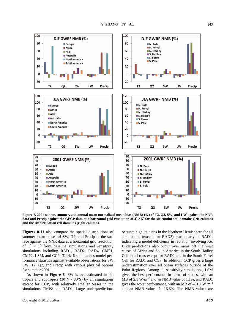
Y. ZHANG ET AL. 243

Figure 7. 2001 winter, summer, and annual mean normalized mean bias (NMB) (%) of T2, Q2, SW, and LW against the NNR data and Precip against the GPCP data at a horizontal grid resolution of 4˚ × 5˚ for the six continental domains (left column) and the six circulation cell domains (right column). Figures 8-11 also compare the spatial distributions of summer mean biases of SW, T2, and Precip at the sur-face against the NNR data at a horizontal grid resolution of 1˚ × 1˚ from baseline simulations and sensitivity simulations including RAD1, RAD2, RAD4, CMP1, CMP2, LSM, and CCP. Table 6 summarizes model performance statistics against available observations for SW, LW, T2, Q2, and Precip with various physical options for summer 2001.

As shown in Figure 8, SW is overestimated in the tropics and subtropics (30˚N - 30˚S) by all simulations except for CCP, with relatively smaller biases in the simulations CMP2 and RAD1. Large underpredictions

occur at high latitudes in the Northern Hemisphere for all simulations (except for RAD2), particularly in RAD1, indicating a model deficiency in radiation involving ice. Underpredictions also occur over areas off the west coasts of Africa and South America in the South Hadley Cell in all runs except for RAD2 and in the South Ferrel Cell for RAD1 and CCP. In addition, CCP gives a large underestimation over all ocean surfaces outside of the Polar Regions. Among all sensitivity simulations, LSM gives the best performance in terms of statics, with an MB of 2.1 W·m–2 and an NMB value of 1.1%, and RAD1 gives the worst performance, with an MB of –31.7 W·m–2 and an NMB value of –16.6%. The NMB values are


Y. ZHANG ET AL. 244

BASE Low_Res RAD1

W·m–2

W·m–2

W·m–2

RAD2 RAD3 CMP1

W·m–2

W·m–2

W·m–2

CMP2 LSM CCP

W·m–2

W·m–2

W·m–2

Figure 8. 2001 summer mean bias plot of downward shortwave fluxes at the surface against NNR data at a horizontal grid resolution of 1˚ × 1˚ from the baseline, RAD1, RAD2, RAD4, CMP1, CMP2, LSM, and CCP simulations and at a horizontal grid resolution of 4˚ × 5˚ from the Low_Res simulation.

BASE Low_Res RAD1

W·m–2

W·m–2

W·m–2

RAD2 RAD3 CMP1

W·m–2

W·m–2

W·m–2

CMP2 LSM CCP

W·m–2

W·m–2

W·m–2

Figure 9. 2001 summer mean bias plot of downward longwave fluxes at the surface against NNR data at a horizontal grid resolution of 1˚ × 1˚ from the baseline, RAD1, RAD2, RAD4, CMP1, CMP2, LSM, and CCP simulations and at a horizontal grid resolution of 4˚ × 5˚ from the Low_Res simulation.


Y. ZHANG ET AL. 245

Baseline Low_Res RAD1

RAD2 RAD3 CMP1

CMP2 LSM CCP

Figure 10. 2001 summer mean bias plot of temperatures at 2-m against NNR data at a horizontal grid resolution of 1˚ × 1˚ from the baseline, RAD1, RAD2, RAD4, CMP1, CMP2, LSM, and CCP simulations and at a horizontal grid resolution of 4˚ × 5˚ from the Low_Res simulation.

Baseline Low_Res RAD1

mm·day–1

mm·day–1

mm·day–1

RAD2 RAD3 CMP1

mm·day–1

mm·day–1

mm·day–1

CMP2 LSM CCP

mm·day–1

mm·day–1 mm·day–1

Figure 11. 2001 summer mean bias plot of daily mean precipitation rate against NNR data at a horizontal grid resolution of 1˚ × 1˚ from the baseline, RAD1, RAD2, RAD4, CMP1, CMP2, LSM, and CCP simulations and at a horizontal grid resolution of 4˚ × 5˚ from the Low_Res simulation.


Y. ZHANG ET AL. 246

Table 6. Performance statistics of GWRF baseline and sensitivity simulations for summer at 1˚ × 1˚ on a global scale.

Variable Dataset Run Mean Obs Mean Mod Number Corr MB RMSE NMB (%) NME (%)

NNR Base 191.34 198.94 61,560 0.93 7.59 41.34 3.97 15.08

RAD1 191.34 159.61 61,560 0.88 –31.74 60.51 –16.59 23.42

RAD2 191.34 200.68 61,560 0.95 9.34 34.74 4.88 12.53

RAD3 191.34 194.71 61,560 0.95 3.37 35.66 1.76 12.85

CMP1 191.34 186.97 61560 0.91 –4.37 45.79 –2.28 17.26

CMP2 191.34 161.60 61,560 0.92 –29.75 50.79 –15.55 19.60

LSM 191.34 193.49 61,560 0.91 2.14 46.03 1.12 17.30

CCP 191.34 164.26 61,560 0.91 –27.09 52.73 –14.16 20.09

OPT 191.34 152.94 61,560 0.91 –38.40 58.52 –20.07 22.65

BSRN Base 218.83 270.32 29 0.98 51.50 57.07 23.53 23.53

RAD1 218.83 226.99 29 0.98 8.16 21.08 3.73 8.19

RAD2 218.83 268.67 29 0.97 49.85 54.95 22.78 22.78

RAD3 218.83 261.92 29 0.98 43.09 48.51 19.69 19.69

CMP1 218.83 259.31 29 0.98 40.48 46.18 18.50 18.70

CMP2 218.83 210.63 29 0.96 –8.20 24.55 –3.75 8.85

LSM 218.83 272.21 29 0.97 53.38 60.70 24.40 24.40

SW (W·m–2)

CCP 218.83 244.39 29 0.93 25.57 47.45 11.68 18.82

NNR Base 306.45 293.76 64,080 0.98 –12.68 24.30 –4.14 6.65

RAD1 306.45 284.53 64,080 0.98 –21.92 29.67 –7.15 8.49

RAD2 306.45 314.42 64,080 0.99 7.98 16.65 2.60 4.12

RAD3 306.45 293.36 64,080 0.98 –13.08 23.61 –4.27 6.47

CMP1 306.45 304.02 64,080 0.98 –2.42 23.38 –0.79 6.34

CMP2 306.45 336.00 64,080 0.97 29.55 51.81 9.64 11.66

LSM 306.45 295.86 64,080 0.98 –10.59 23.88 –3.45 6.64

CCP 306.45 306.73 64,080 0.98 0.28 21.18 0.09 5.80

OPT 306.45 335.14 64,080 0.98 28.69 33.55 9.36 9.57

BSRN Base 350.01 317.91 29 0.93 –32.10 39.63 –9.17 9.17

RAD1 350.01 306.27 29 0.93 –43.74 49.36 –12.50 12.50

RAD2 350.01 342.29 29 0.93 –7.72 25.11 –2.21 4.64

RAD3 350.01 317.48 29 0.92 –32.53 40.56 –9.29 9.33

CMP1 350.01 325.69 29 0.93 –24.32 32.81 –6.95 7.28

CMP2 350.01 358.23 29 0.92 8.22 28.07 2.35 5.74

LSM 350.01 316.50 29 0.92 –33.51 40.97 –9.57 9.73

LW (W·m–2)

CCP 350.01 323.15 29 0.92 –26.86 38.18 –7.67 8.76


Y. ZHANG ET AL. 247

Continued

NNR Base 7.48 7.68 64,079 0.99 0.20 2.33 2.70 18.75

RAD1 7.48 6.31 64,079 0.99 –1.17 3.02 –15.64 27.34

RAD2 7.48 8.08 64,079 0.99 0.60 2.47 8.01 20.61

RAD3 7.48 7.49 64,079 0.99 0.01 2.28 0.14 18.84

CMP1 7.48 7.45 64,079 0.99 –0.03 2.38 –0.38 20.58

CMP2 7.48 11.77 64,078 0.96 4.29 10.59 57.30 62.08

LSM 7.48 7.48 64,079 0.99 0.01 2.61 0.07 20.72

CCP 7.48 6.74 64,079 0.99 –0.74 2.34 –9.92 20.65

OPT 7.48 7.90 64,078 0.99 0.42 2.85 5.60 23.22

NCDC Base 20.77 20.27 199 0.88 –0.51 4.18 –2.43 12.24

RAD1 20.78 17.78 199 0.86 –3.00 5.33 –14.43 20.15

RAD2 20.78 21.60 199 0.87 0.82 4.36 3.95 12.01

RAD3 20.78 20.21 199 0.88 –0.57 4.18 –2.73 12.26

CMP1 20.78 19.96 199 0.88 –0.81 4.21 –3.91 12.63

CMP2 20.78 20.74 199 0.86 –0.03 4.24 –0.17 11.49

LSM 20.78 19.84 199 0.89 –0.94 4.04 –4.50 11.77

T2 (˚C)

CCP 20.78 19.41 199 0.88 –1.37 4.42 –6.58 14.05

NNR Base 8.85 8.64 64,080 0.99 –0.21 1.03 –2.39 7.12

RAD1 8.85 8.19 64,080 0.98 –0.66 1.46 –7.45 10.29

RAD2 8.85 8.63 64,080 0.99 –0.22 0.85 –2.52 5.78

RAD3 8.85 8.64 64,080 0.99 –0.21 1.04 –2.39 7.41

CMP1 8.85 8.70 64,080 0.99 –0.15 1.00 –1.74 7.09

CMP2 8.85 9.91 64,080 0.98 1.06 1.69 11.96 13.04

LSM 8.85 9.17 64,080 0.98 0.31 1.27 3.52 7.86

CCP 8.85 8.37 64,080 0.99 –0.49 1.07 –5.49 7.39

Q2 (g·kg–1)

OPT 8.85 9.16 64,080 0.97 0.30 1.46 3.42 8.29

GPCP Base 2.22 3.08 10,363 0.83 0.86 1.96 38.64 54.4

RAD1 2.22 3.05 10,363 0.79 0.83 2.13 37.15 55.11

RAD2 2.22 3.22 10,362 0.74 0.99 2.59 44.62 63.86

RAD3 2.22 2.87 10,361 0.79 0.65 1.94 29.12 50.79

CMP1 2.22 3.00 10,363 0.80 0.77 1.91 34.77 53.57

CMP2 2.22 9.66 10,363 0.60 7.44 8.18 334.31 335.37

LSM 2.22 3.00 10,362 0.73 0.78 2.33 35.08 57.12

CCP 2.22 2.72 10,363 0.73 0.49 1.78 22.10 50.87

OPT 2.22 2.65 10,363 0.70 0.42 1.83 19.08 51.53

NCDC Base 93.20 116.77 172 0.67 23.57 88.50 25.29 58.48

RAD1 93.20 98.90 172 0.70 5.70 77.26 6.12 49.58

RAD2 93.20 125.36 172 0.60 32.16 110.75 34.51 70.19

RAD3 93.20 104.72 172 0.72 11.52 78.91 12.36 49.61

CMP1 93.20 111.67 172 0.66 18.48 89.37 19.83 56.85

CMP2 91.20 284.69 172 0.60 191.50 219.92 205.48 213.91

LSM 93.20 99.74 172 0.67 6.54 81.80 7.02 49.14

Precip (mm·d–1)

CCP 93.20 93.86 172 0.54 0.66 96.05 0.71 54.95

SW—Downward shortwave radiative flux at surface; LW—Downward longwave flux at surface; T2—Temperature at 2-m; Q2—Water vapor mixing ratio at -m; Precip—Daily mean precipitation rate. 2


Y. ZHANG ET AL.


248

within ±5% for BASE, RAD2, RAD3, and CMP1, indicating a similar performance by the simulations with the Goddard and CAM shortwave radiation schemes, or the RRTM and CAM longwave radiation schemes, or the WSM3 and WSM6 cloud microphysics schemes. Larger biases in SW by RAD1, CMP2, and CCP indicate a poor performance of the combination of the schemes that include the Dudhia shortwave scheme or the Purdue Lin cloud microphysics scheme, or the Grell-Devenyi cumulus parameterization, as compared with their respective schemes used in BASE. Compared with the BSRN data, RAD1 performs the best among all simulations and much better than BASE (with MB values of 8.2 vs. 51.5 W·m–2, and NMBs of 3.7% vs. 23.5%). CMP2 also performs well, with an NMB of –3.8%.

For LW, NMBs are within ±10% against the NNR data for all simulations. CCP, CMP1, and RAD2 show a better performance against the NNR data than other simulations, with NMBs of 0.1%, –0.8%, and 2.6%, re-spectively. Among all simulations, CMP2 gives the worst performance with an NMB of 9.6% and the largest biases occurring over Antarctic and Greenland as shown in Figure 9, indicating a high sensitivity of LW to the cloud microphysics over these areas. As shown in Figure 9, LW over most tropics and mid-latitude areas is underpredicted from all simulations except for RAD2 and CMP2. LW radiation flux over high latitudes is overpre-dicted except for Arctic from RAD1. RAD2 and CMP2 overpredict LW radiation flux over most of the domain. NMBs are also within ±10% against BSRN data for all simulations except for RAD1. RAD2 and CMP2 show better performance against BSRN than other simulations, with NMBs of 2.2% and 2.4%, respectively. BASE and RAD2 give MB values of –12.7 and 8.0 W·m–2 against NNR and –32.10 and –7.72 W·m–2 against BSRN, re-spectively, indicating that the combination of schemes that include the RRTM longwave module is more accu- rate in simulating longwave radiation than that includes the CAM longwave module under summer conditions.

For T2, three simulations, LSM, RAD3, and CMP1 show better performance and CMP2 shows the worst performance against the NNR data. CMP2, BASE, and RAD3 show better performance and RAD1 shows the worst performance against the NCDC data. As shown in Figures 9 and 10, the large overpredictions of T2 by CMP2 and RAD2 are clearly related to overpredictions of LW from both simulations. Compared with results from BASE, LSM shows smaller overpredictions over land areas except for a few areas including the Greenland, Saudi Arabia, and Iran where LSM shows a larger under prediction than BASE. This indicates that the Slab LSM performs well under summer conditions, as compared with the NOAH LSM used in BASE. RAD3 and CMP1 show smaller overpredictions over several regions in

cluding North America and Russia, indicating a good performance by the CAM shortwave radiation scheme and by the WSM6 microphysics module. In contrast to all other simulations, RAD1 underpredicts T2 over most land areas (except for South Asia), particularly over Rus- sia and northeastern China, which is likely caused by large underpredictions of SW radiation flux over high latitudes in Northern Hemisphere as shown in Figure 8 and underpredictions of LW radiation flux over most of the domain except for South Pole and South Ferrel as shown in Figure 9. The worst performance in T2 predic-tions by CMP2 against the NNR data is caused by large overpredictions of LW radiation fluxes over the South Ferrel cell, South Pole, and Greenland. The errors over the poles are not reflected in the statistics of CMP2 against NCDC because there is no station in Greenland and only 3 out of the 199 stations are in Antarctica. These results indicate a poor performance in T2 predic-tions by the combination of the schemes that includes Dudhia shortwave radiation scheme (i.e. RAD1) or the Purdue Lin microphysics module (i.e. CMP2) under summer conditions.

Compared with BASE, For Q2, all NMBs are within 5% against NNR data except for CMP2 and RAD1. For Precip, all simulations overpredict against the GPCP data, with the least overpredictions by CCP and RAD3 (NMBs of 22.1% and 29%, respectively) and the worst overpredictions by CMP2 (NMB of 334.3%). Compared with the NCDC data, Precip is also overpredicted, with a small overprediction by CCP, RAD1, and LSM (NMBs of 0.7%, 6.1%, and 7%, respectively) and the largest overprediction by CMP2 (NMB of 205.5%). As shown in Figure 11, overpredictions occur over nearly the entire domain by CMP2 and over most areas except for the South Ferrel cell and South Pole by other simulations. The poor performance of CMP2 indicates that the defi-ciency of the combination of schemes that include the Purdue-Lin microphysics parameterization in simulating precipitation under the summer conditions.

Given high sensitivity of the model predictions to various physical options, in particular, SW radiation scheme, cloud microphysics, and cumulus parameteriza-tion, an additional sensitivity simulation is performed using the best schemes or parameterizations identified through the above sensitivity simulations. The overall best schemes identified include the CAM shortwave scheme in terms of SW, T2, Q2, Precip (by comparing BASE, RAD1, and RAD3), the RRTM longwave scheme in terms of LW (by comparing RAD2 and RAD3), the WSM6 microphysics module in terms of SW, LW, T2, Q2, and Precip (by comparing BASE, CMP1, and CMP2), the Slab LSM (by comparing BASE and LSM), and the Grell-Devenyi cumulus parameterization in terms of Precip (comparing BASE and CCP). A sensitivity

Y. ZHANG ET AL. 249

simulation using these schemes is performed (referred to as OPT in Table 6). OPT shows the best performance in Precip among all simulations, with an NMB of 19.1 against GPCP (comparing to 22.1% - 334.3% by other simulations). However, given a non-linearity of the in-teractions among various schemes, OPT does not show the best performance for other meteorological variables. For example, it gives an NMB of –20.1% for SW, 9.4% for LW, 5.6% for T2, and 3.4% for Q2 against the NNR data.

6. Future Year Simulations

A simulation for the year of 2050 are performed at a horizontal grid resolution of 4˚ × 5˚ and compared with the 2001 results from Low_Res. Under the SRES B1 climate scenario, global mean values of LW, T2, and Q2 increase and those of SW, wind speed at 10-m, PBL height, and Precip decrease. Figure 12 shows the annual mean absolute changes in T2 and Precip between 2050 and 2001. In response to ~51% increases in CO2 mixing ratios, T2 increases by up to 5.2˚C over most areas in the global domain except for a few areas including the South Pole, South Ferrel cell, and Atlantic ocean where T2 may

decrease by as much as 6.2˚C, with a net increase of ~0.2˚C on a global mean. The largest increases in T2 occur over southern South Africa, East Asia, southern Nouth Amercia, nothern South Amercia, and some areas in the North Ferrel cell. Precip in 2050 decreases over most areas, with the largest decrease of 8.2 mm·day–1 occuring over the tropics between 60˚E - 160˚E. Precip increases over the southern China, central Africa, Aus-tralia, a large area over the Pacific ocean and some areas over the Atlantic ocean in the southern hemisphere. The net change is a decrease in global mean precipitation amount by ~0.5 mm·day–1. The projected changes are generally consistent with other GCM predictions in terms of both magnitudes and spatial distributions (e.g. [62]).

7. Conclusions

The ability of GWRF in reproducing observations of major boundary layer meteorological variables is evalu-ated by comparing the 2001 model predictions with data from observational networks (e.g. NCDC and BSRN) and gridded Reanalysis data (e.g. NNR and GPCP). GWRF at a horizontal grid resolution of 1˚ × 1˚ shows small biases against the NNR data and moderate over-

T2

Precip mm·day–1

Figure 12. Projected absolute changes in tempreatue and precipitation in 2050 relative to 2001 at a horizontal grid resolution f 4˚ × 5˚. o


Y. ZHANG ET AL. 250

predictions against the BSRN data in the SW predictions. LW is slightly underpredicted against both the NNR and BSRN. T2 is underpredicted against the NNR and NCDC data in both summer and winter, with larger cold biases against the NCDC data (MBs as large as –2.3˚C). Q2 is slightly underpredicted against the NNR data. Larger biases exist in wind speed and precipitation predictions, with large underpredictions in U10 against the NNR data and large overpredictions in Precip against the GPCP and NCDC data. The performance of GWRF in predicting major meteorological variables is overall consistent with that of most current GCMs.

Among all major variables examined, GWRF shows a large sensitivity to horizontal grid resolution for T2 predictions in winter and for Precip predictions in winter and summer. The model simulation at a coarser resolution leads to a much worse overprediction of T2 over the North America and a much less overprediction over the North Ferrel cell in winter. It also gives a worse agreement with observations for Precip over the most continents and most circulation cells during winter and sum-mer. The sensitivity simulations using various physical options show a poor performance in SW, T2, and Q2 predictions by the combination of schemes that includes the Dudhia shortwave radiation scheme, or the Purdue Lin microphysics module, or the Grell-Devenyi cumulus parameterization, and in Precip predictions by the combination of schemes that includes the Purdue Lin microphysics module. These simulations identify that CAM, RRTM, WSM6, Slab, and Grell-Devenyi represent the best shortwave, longwave, cloud microphysics, land- surface, and cumulus treatments. While the simulation with these best schemes/parameterizations gives the best performance in Precip predictions by reducing the NMB of Precip from 38.6% to 19.1%, it does not give the best performance for all other major meteorological variables, because of a complex interaction of various atmospheric processes. A one-year simulation of GWRF for 2050 indicates a projected warmer and drier future climate. The projected future climate change may have important im-plications on the fate and lifetime of air pollutants. For example, decreased precipitation will reduce the scav- enging rate of air pollutants, and decreased wind speeds and PBL height will increase the concentrations of air pollutant via reduced ventilation. The impact of future climate change on future air quality is being studied using a coupled GWRF and chemistry model and the results will be reported in a separate paper [63,64].

8. Acknowledgements

This research was supported by EPA STAR grant #R8337601, US Department of Energy grant #DE-FG02- 08ER64508, and China’s National Basic Research Pro- gram (2010CB951803). Thanks are due to Jimmy Dudia,

NCAR, for his valuable suggestions on the selection of the cumulus parameterization; and Brett Gantt, a gradu- ate student at NCSU, for his help in improving the quality of Figures 3 and 7.

REFERENCES

[1] W. C. Skamarock, J. B. Klemp, J. Dudhia, D. O. Gill, D. M. Barker, W. Wang and J. G. Powers, “A Description of the Advanced Research WRF Version 2,” National Center for Atmospheric Research Technical Note, NCAR, Boul-der, 2007. http://www.mmm.ucar.edu/wrf/users/docs/arw_v2.pdf

[2] W. C. Skamarock, J. B. Klemp, J. Dudhia, D. O. Gill, D. M. Barker, M. G. Duda, X.-Y. Huang, W. Wang and J. G. Powers, “A Description of the Advanced Research WRF Version 3,” National Center for Atmospheric Research Technical Note, NCAR, Boulder, 2008. http://www.mmm.ucar.edu/wrf/users/docs/arw_v3.pdf

[3] Y. V. R. Rao, H. R. Hatwar, A. K. Salah and Y. Sudhakar, “An Experiment Using the High Resolution Eta and WRF Models to Forecast Heavy Precipitation over India,” Pure and Applied Geophysics, Vol. 164, No. 8-9, 2007, pp. 1593-1615. doi:10.1007/s00024-007-0244-1

[4] H. Wang, W. C. Skamarock and G. Feingold, “Evaluation of Scalar Advection Schemes in the Advanced Research WRF Model Using Large-Eddy Simulations of Aero-sol-Cloud Interaction,” Monthly Weather Review, Vol. 137, No. 8, 2009, pp. 2547-2558. doi:10.1175/2009MWR2820.1

[5] W. C. Skamarock and J. B. Klemp, “A Time-Split Non-Hydrostatic Atmospheric Model for Research and NWP Applications,” Journal of Computational Physics: Special Issue on Environmental Modeling, Vol. 227, No. 7, 2008, pp. 3465-3485.

[6] X.-G. Wang, D. M. Barker, C. Snyder and T. M. Hamill, “A Hybrid ETKF—3DVAR Data Assimilation Scheme for the WRF Model. Part I: Observing System Simulation Experiment,” Monthly Weather Review, Vol. 136, No. 12, 2008, pp. 5116-5131. doi:10.1175/2008MWR2444.1

[7] X.-Y. Huang, et al., “Four-Dimensional Variational Data Assimilation for WRF: Formulation and Preliminary Re-sults,” Monthly Weather Review, Vol. 137, No. 1, 2009, pp. 299-314. doi:10.1175/2008MWR2577.1

[8] L. R. Leung, Y.-H. Kuo and J. Tribbia, “Research Needs and Directions of Regional Climate Modeling Using WRF and CCSM,” Bulletin of the American Meteoro-logical Society, Vol. 87, No. 12, 2006, pp. 1747-1751. doi:10.1175/BAMS-87-12-1747

[9] X.-Z. Liang, M. Xu, K. E. Kunkel, G. A. Grell and J. S. Kain, “Regional Climate Model Simulation of US Mex- ico Summer Precipitation Using the Optimal Ensemble of Two Cumulus Parameterizations,” Journal of Climate, Vol. 20, No. 20, 2007, pp. 5201-5207. doi:10.1175/JCLI4306.1

[10] M. S. Bukovsky and D. J. Karoly, “Precipitation Simula-tions Using WRF as a Nested Regional Climate Model,” Journal of Climate and Applied Meteorology, Vol. 48, No.


Y. ZHANG ET AL. 251

10, 2009, pp. 2152-2159. doi:10.1175/2009JAMC2186.1

[11] L. R. Leung and Y. Qian, “Atmospheric Rivers Induced Heavy Precipitation and Flooding in the Western US Simulated by the WRF Regional Climate Model,” Geo- physical Research Letters, Vol. 36, 2009, Article ID: L03820.

[12] C. Zhao, X. Liu, L. Y. R. Leung and S. M. Hagos, “Ra- diative Impact of Mineral Dust on Monsoon Precipitation Variability over West Africa,” Atmospheric Chemistry and Physics, Vol. 11, No. 5, 2011, pp. 1879-1893. doi:10.5194/acp-11-1879-2011

[13] G. A. Grell, S. E. Peckham, R. Schmitz, S. A. McKeen, G. Frost, W. C. Skamarock and B. Eder, “Fully Coupled Online ‘Chemistry’ within the WRF Model,” Atmos- pheric Environment, Vol. 39, No. 37, 2005, pp. 6957- 6975. doi:10.1016/j.atmosenv.2005.04.027

[14] J. D. Fast Jr., W. I. Gustafson, R. C. Easter, R. A. Zaveri, J. C. Barnard, E. G. Chapman and G. A. Grell, “Evolution of Ozone, Particulates, and Aerosol Direct Forcing in an Urban Area Using a New Fully-Coupled Meteorology, Chemistry, and Aerosol Model,” Journal of Geophysical Research, Vol. 111, 2006, Article ID: D21305. doi:10.1029/2005JD006721

[15] E. G. Chapman Jr., W. I. Gustafson, R. C. Easter, J. C. Barnard, S. J. Ghan, M. S. Pekour and J. D. Fast, “Cou-pling Aerosol-Cloud-Radiative Processes in the WRF- Chem Model: Investigating the Radiative Impact of Ele- vated Point Sources,” Atmospheric Chemistry Physics, Vol. 9, 2009, pp. 945-964. doi:10.5194/acp-9-945-2009

[16] C. Misenis and Y. Zhang, “An Examination of WRF/ Chem: Physical Parameterizations, Nesting Options, and Grid Resolutions,” Atmospheric Research, Vol. 97, No. 3, 2010, pp. 315-334. doi:10.1016/j.atmosres.2010.04.005

[17] Y. Zhang, X.-Y. Wen and C. J. Jang, “Simulating Cli-mate-Chemistry-Aerosol-Cloud-Radiation Feedbacks in Continental US Using Online-Coupled Weather Research Forecasting Model with Chemistry (WRF/Chem),” At- mospheric Environment, Vol. 44, No. 29, 2010, pp. 3568- 3582. doi:10.1016/j.atmosenv.2010.05.056

[18] Y. Zhang, Y. Pan, K. Wang, J. D. Fast and G. A. Grell, “WRF/Chem-Madrid: Incorporation of an Aerosol Mod-ule into WRF/Chem and Its Initial Application to the TexAQS2000 Episode,” Journal of Geophysical Re- search, Vol. 115, 2010, Article ID: D18202. doi:10.1029/2009JD013443

[19] S. McKeen, J. Wilczak, G. Grell, I. Djalalova, S. Peckham, E.-Y. Hsie, W. Gong, V. Bouchet, S. Menard, R. Moffet, J. McHenry, J. McQueen, Y. Tang, G. R. Carmichael, M. Pagowski, A. Chan, T. Dye, G. Frost, P. Lee and R. Mathur, “Assessment of an Ensemble of Seven Real-Time Ozone Forecasts over Eastern North America during the Summer of 2004,” Journal of Geophysical Research, Vol. 110, 2005, Article ID: D21307. doi:10.1029/2005JD005858

[20] S. Mckeen, S. H. Chung, J. Wilczak, G. Grell, I. Djalalova, S. Peckhamm, W. Gong, V. Bouchet, R. Moffet, Y. Tang, G. R. Carmichael, R. Mathur and S. Yu, “Evaluation of Several PM2.5 Forecast Models Using Data Collected during the ICARTT/NEAQS 2004 Field Study,” Journal of Geophysical Research, Vol. 112, 2007, Article ID: D10S20.

doi:10.1029/2006JD007608

[21] L. D. Monache, J. Wilczak, S. McKeen, G. Grell, M. Pagowski, S. Peckham, R. Stoll, J. McHenry and J. McQueen, “A Kalman-Filter Bias Correction Method Ap- plied to Deterministic, Ensemble Averaged, and Prob- abilistic Forecasts of Surface Ozone,” Tellus, Vol. 60, No. 2, 2007. doi:10.1111/j.1600-0889.2007.00332.x

[22] M.-T. Chuang, Y. Zhang and D. Kang, “Application of WRF/Chem-Madrid for Real-Time Air Quality Forecast- ing over the Southeastern United States,” Atmospheric Environment, Vol. 45, No. 34, 2011, pp. 6241-6250. doi:10.1016/j.atmosenv.2011.06.071

[23] S. Chen, J. F. Price, W. Zhao, M. A. Donelan and E. J. Walsh, “The CBLAST-Hurricane Program and the Next- Generation Fully Coupled Atmosphere-Wave-Ocean Mo- dels for Hurricane Research and Prediction, March,” Bul- letin of the American Meteorological Society, Vol. 88, No. 3, 2007, pp. 311-317. doi:10.1175/BAMS-88-3-311

[24] B. Liu, H.-Q. Liu, L. Xie, C.-L. Guan and D.-L. Zhao, “A Coupled Atmosphere-Wave-Ocean Modeling System: Simulation of the Intensity of an Idealized Tropical Cy- clone,” Monthly Weather Review, Vol. 139, No. 1, 2011, pp. 132-152. doi:10.1175/2010MWR3396.1

[25] M. I. Richardson, A. D. Toigo and C. E. Newman, “Non- Conformal Projection, Global, and Planetary Versions of WRF,” 6th WRF/15th MM5 User’s Workshop, Boulder, 27-30 June 2005.

[26] M. I. Richardson, A. D. Toigo and C. E. Newman, “Pla- net WRF: A General Purpose, Local to Global Numerical Model for Planetary Atmosphere and Climate Dynamics,” Journal of Geophysical Research, Vol. 112, 2007, Article ID: E09001. doi:10.1029/2006JE002825

[27] M. A. Mischna, M. Allen, M. I. Richardson, C. E. Newman and A. D. Toigo, “Atmospheric Modeling of Mars Meth-ane Surface Releases,” Planetary and Space Science, Vol. 59, No. 2-3, 2011, pp. 227-237. doi:10.1016/j.pss.2010.07.005

[28] W. D. Collins, et al., “Description of the NCAR Commu- nity Atmosphere Model (CAM 3.0),” National Center for Atmospheric Research Technical Note, NCAR, Boulder, 2004.

[29] E. J. Mlawer, S. J. Taubman, P. D. Brown, M. J. Iacono and S. A. Clough, “Radiative Transfer for Inhomogeneous Atmospheres: RRTM, a Validated Correlated-k Model for the Longwave,” Journal of Geophysical Research, Vol. 102, No. D14, 1997, pp. 16663-16682. doi:10.1029/97JD00237

[30] M.-D. Chou and M. J. Suarez, “An Efficient Thermal In- frared Radiation Parameterization for Use in General Circulation Models,” NASA Technical Memorandum, Vol. 3, 1994, Article ID: 104606.

[31] M. D. Chou, M. J. Suarez, C. H. Ho, M. M. H. Yan and K. T. Lee, “Parameterizations for Cloud Overlapping and Shortwave Single-Scattering Properties for Use in Gen- eral Circulation and Cloud Ensemble Models,” Journal of Climate, Vol. 11, No. 2, 1998, pp. 202-214. doi:10.1175/1520-0442(1998)011<0202:PFCOAS>2.0.CO;2

[32] J. Dudhia, “Numerical Study of Convection Observed


Y. ZHANG ET AL. 252

during the Winter Monsoon Experiment Using a Meso- scale Two-Dimensional Model,” Journal of Atmospheric Sciences, Vol. 46, No. 20, 1989, pp. 3077-3107. doi:10.1175/1520-0469(1989)046<3077:NSOCOD>2.0.CO;2

[33] Y.-L. Lin, R. D. Farley and H. D. Orville, “Bulk Parame- terization of the Snow Field in a Cloud Model,” Journal of Climate and Applied Meteorology, Vol. 22, No. 6, 1983, pp. 1065-1092. doi:10.1175/1520-0450(1983)022<1065:BPOTSF>2.0.CO;2

[34] S.-H. Chen and W.-Y. Sun, “A One-Dimensional Time Dependent Cloud Model,” Journal of the Meteorological Society of Japan, Vol. 80, No. 1, 2002, pp. 99-118. doi:10.2151/jmsj.80.99

[35] K.-S. Lim and S.-Y. Hong, “A New Double Moment Approach for the Warm-Rain Process Based on the WSM6 Scheme (WDM6),” The 9th WRF User’s Work-shop, Boulder, 23-27 June 2008.

[36] F. Chen and J. Dudhia, “Coupling an Advanced Land Surface-Hydrology Model with the Penn State-NCAR MM5 Modeling System. Part I: Model Implementation and Sensitivity,” Monthly Weather Review, Vol. 129, No. 4, 2001, pp. 569-585. doi:10.1175/1520-0493(2001)129<0569:CAALSH>2.0.CO;2

[37] F. Chen and J. Dudhia, “Coupling an Advanced Land Surface-Hydrology Model with the Penn State-NCAR MM5 Modeling System. Part II: Preliminary Model Validation,” Monthly Weather Review, Vol. 129, No. 4, 2001, pp. 587-604. doi:10.1175/1520-0493(2001)129<0587:CAALSH>2.0.CO;2

[38] M. B. Ek, K. B. Mitchell, Y. Lin, B. Rogers, P. Grun-mann, V. Koren, G. Gayno and J. D. Tarpley, “Imple-mentation of Noah Land Surface Model Advances in the National Centers for Environmental Prediction Opera-tional Mesoscale Eta Model,” Journal of Geophysical Research, Vol. 108, 2003. doi:10.1029/2002JD003296

[39] J. Dudhia, “A Multi-Layer Soil Temperature Model for MM5,” Sixth PSU/NCAR Mesoscale Model Users’ Work- shop, Boulder, 22-24 July 1996, pp. 49-50.

[40] J. S. Kain and J. M. Fritsch, “A One Dimensional En- training/Detraining Plume Model and Its Application in Convective Parameterization,” Journal of Atmospheric Sciences, Vol. 47, No. 23, 1990, pp. 2784-2802. doi:10.1175/1520-0469(1990)047<2784:AODEPM>2.0.CO;2

[41] J. S. Kainand and J. M. Fritsch, “Convective Parameteri- zation for Mesoscale Models: The Kain-Fritsch Scheme,” In: J. S. Kainand and J. M. Fritsch, Eds., The Representa- tion of Cumulus Convection in Numerical Models, Ame- rican Meteorological Society, Boston, 1993, pp. 165-170.

[42] J. S. Kain, “The Kain-Fritsch Convective Parameteriza- tion: An Update,” Journal of Applied Meteorology, Vol. 43, No. 1, 2004, pp. 170-181. doi:10.1175/1520-0450(2004)043<0170:TKCPAU>2.0.CO;2

[43] G. A. Grell and D. Devenyi, “A Generalized Approach to

Parameterizing Convection Combining Ensemble and Data Assimilation Techniques,” Geophysical Research Letters, Vol. 29, 2002, pp. 1693-1696. doi:10.1029/2002GL015311

[44] S.-Y. Hong and J. Dudhia, “Testing of a New Non-Local Boundary Layer Vertical Diffusion Scheme in Numerical Weather Prediction Applications,” The 20th Conference on Weather Analysis and Forecasting/16th Conference on Numerical Weather Prediction, Seattle, 10-12 January 2004.

[45] S. Hong, Y. Noh and J. Dudhia, “A New Vertical Diffu- sion Package with an Explicit Treatment of Entrainment Processes,” Monthly Weather Review, Vol. 134, No. 9, 2006, pp. 2318-2341. doi:10.1175/MWR3199.1

[46] S.-Y. Hong, S.-W. Kim, J. Dudhia and M.-S. Koo, “Sta- ble Boundary Layer Mixing in a Vertical Diffusion Pack- age,” The 9th Annual of WRF Workshop, Boulder, 23-27 June 2008.

[47] A. S. Monin, and A. M. Obukho, “Basic Laws of Turbu- lent Mixing in the Surface Layer of the Atmosphere,” Contributions of the Geophysical Institute of the Academy of Sciences, Vol. 24, No. 151, 1954, pp. 163-187.

[48] D.-L. Zhang and R. A. Anthes, “A High-Resolution Mo- del of the Planetary Boundary Layer-Sensitivity Tests and Comparisons with SESAME-79 Data,” Journal of Ap-plied Meteorology, Vol. 21, No. 11, 1982, pp. 1594-1609.

[49] C. A. Paulson, “The Mathematical Representation of Wind Speed and Temperature Profiles in the Unstable Atmos- pheric Surface Layer,” Journal of Applied Meteorology, Vol. 9, No. 6, 1970, pp. 857-861. doi:10.1175/1520-0450(1970)009<0857:TMROWS>2.0.CO;2

[50] A. J. Dyer and B. B. Hicks, “Flux-Gradient Relationships in the Constant Flux Layer,” Quarterly Journal of the Royal Meteorological Society, Vol. 96, No. 410, 1970, pp. 715-721. doi:10.1002/qj.49709641012

[51] E. K. Webb, “Profile Relationships: The Log-Linear Range, and Extension to Strong Stability,” Quarterly Journal of the Royal Meteorological Society, Vol. 96, No. 407, 1970, pp. 67-90. doi: 10.1002/qj.49709640708

[52] A. Ohmura, et al., “Baseline Surface Radiation Network (BSRN/WCRP): New Precision Radiometry for Climate,” Bulletin of the American Meteorological Society, Vol. 79, No. 10, 1998, pp. 2115-2136. doi:10.1175/1520-0477(1998)079<2115:BSRNBW>2.0.CO;2

[53] P. Xie and P. Arkin, “Global Precipitation: A 17-Year Monthly Analysis Based on Gauge Observations, Satellite Estimates, and Numerical Model Outputs,” Bulletin of the American Meteorological Society, Vol. 78, No. 11, 1997, pp. 2539-2558. doi:10.1175/1520-0477(1997)078<2539:GPAYMA>2.0.CO;2

[54] E. Kalnay, et al., “The NCEP/NCAR 40-Year Reanalysis Project,” Bulletin of the American Meteorological Society, Vol. 77, No. 3, 1996, pp. 437-471. doi:10.1175/1520-0477(1996)077<0437:TNYRP>2.0.CO;2

[55] Y. Zhang, P. Liu, B. Pun and C. Seigneur, “A Compre- hensive Performance Evaluation of MM5-CMAQ for the


http://dx.doi.org/10.1029/2002JD003296

Y. ZHANG ET AL.


253

Summer 1999 Southern Oxidants Study Episode, Part-I. Evaluation Protocols, Databases and Meteorological Pre- dictions,” Atmospheric Environment, Vol. 40, No. 26, 2006, pp. 4825-4838. doi:10.1016/j.atmosenv.2005.12.043

[56] M. Wild, A. Ohmura, H. Gilgen and E. Roeckner, “Vali-dation of General Circulation Model Radiative Fluxes Using Surface Observations,” Journal of Climate, Vol. 8, No. 5, 1995, pp. 1309-1324. doi:10.1175/1520-0442(1995)008<1309:VOGCMR>2.0.CO;2

[57] J. H. Christensen, B. Hewitson, A. Busuioc, A. Chen, X. Gao, I. Held, R. Jones, R. K. Kolli, W.-T. Kwon, R. La-prise, V. M. Rueda, L. Mearns, C. G. Menéndez, J. Räi- sänen, A. Rinke, A. Sarr and P. Whetton, “Regional Cli- mate Projections,” In: S. Solomon, D. Qin, M. Manning, Z. Chen, M. Marquis, K. B. Averyt, M. Tignor and H. L. Miller, Eds., Climate Change 2007: The Physical Science Basis. Contribution of Working Group I to the Fourth Assessment Report of the Intergovernmental Panel on Climate Change, Cambridge University Press, Cambridge, 2007.

[58] S. J. Lambert and G. J. Boer, “CMIP1 Evaluation and Intercomparison of Coupled Climate Models,” Climate Dynamics, Vol. 17, No. 2-3, 2001, pp. 83-106. doi:10.1007/PL00013736

[59] D. Bader, “An Appraisal of Coupled Climate Model Si- mulations,” Lawrence Livermore National Laboratory, Livermore, 2004.

[60] D. A. Randall, R. A. Wood, S. Bony, R. Colman, T. Fi- chefet, J. Fyfe, V. Kattsov, A. Pitman, J. Shukla, J. Srini- vasan, R. J. Stouffer, A. Sumi and K. E. Taylor, “Climate Models and Their Evaluation,” In: S. Solomon, D. Qin, M. Manning, Z. Chen, M. Marquis, K. B. Averyt, M. Tignor and H. L. Miller, Eds., Climate Change 2007: The Physi-

cal Science Basis. Contribution of Working Group I to the Fourth Assessment Report of the Intergovernmental Panel on Climate Change, Cambridge University Press, Cam- bridge, 2007.

[61] C. Covey, K. M. AchutaRao, U. Cubasch, P. Jones, S. J. Lambert, M. E. Mann, T. J. Phillips and K. E. Taylor, “An Overview of Results from the Coupled Model Inter- comparison Project (CMIP),” Global and Planetary Change, Vol. 37, No. 1-2, 2003, pp. 103-133. doi:10.1016/S0921-8181(02)00193-5

[62] A. J. G. Baumgaertner, P. Jöckel, M. Dameris and P. J. Crutzen, “Will Climate Change Increase Ozone Depletion Fromlow-Energy-Electron Precipitation?” Atmospheric Che- mistry and Physics, Vol. 10, 2010, pp. 9647-9656. doi:10.5194/acp-10-9647-2010.

[63] Y. Zhang, P. Karamchandani, T. Glotfelty, D. G. Streets, W. C. Skamarock, G. Grell, A. Nenes, F.-Q. Yu and R. Bennartz, “Development and Initial Application of the Global-through-Urban WRF/Chem,” Journal of Geophy- sical Research, 2012, in press.

[64] T. Glotfelty, Y. Zhang, S. Zhu, P. Karamchandani and D. G. Streets, “Assessing the Impact of Changes in Climate and Emission on Global Air Quality,” The 11th Annual CMAS Conference, Chapel Hill, 15-17 October, 2012.

[65] S.-Y. Hong, J. Dudhia and S.-H. Chen, “A Revised Ap- proach to Ice Microphysical Processes for the Bulk Para- meterization of Clouds and Precipitation,” Monthly Wea- ther Review, Vol. 132, No. 1, 2004, pp. 103-120. doi:10.1175/1520-0493(2004)132<0103:ARATIM>2.0.CO;2

[66] S.-Y. Hong and J. O. Lim, “The WRF Single Moment 6- Class Microphysics Scheme (WSM6),” Journal of the Korean Meteorology Society, Vol. 42, No. 2, 2006, pp. 129-151.

The Global Weather Research and Forecasting …file.scirp.org/pdf/ACS20120300006_44268753.pdf ·...

Documents

Transcript of The Global Weather Research and Forecasting …file.scirp.org/pdf/ACS20120300006_44268753.pdf ·...