THE GLOBAL CONVERGENCE OF INCOME

DISTRIBUTION

John Luke Gallup

Portland State University 1721 SW Broadway

Cramer Hall, Suite 241 Portland OR 97201 jlgallup@pdx.edu tel: 503-725-3929 fax: 503-725-3945

September 15, 2012

Abstract

What happens to income distribution during the course of economic development? New

higher quality international data show a marked pattern of inequality convergence, where

inequality becomes more similar across countries as income levels rise. Inequality has

tended to fall in high inequality countries as their economies grow, and inequality has

tended to rise in low inequality countries. This is clear in linear regression trends,

piecewise trends, and stochastic kernel estimation. The stochastic kernel estimation

models the evolution of inequality in the income domain, rather than the more typical

time domain, and allows for complex dynamics. The evidence of inequality convergence is

confirmed in numerous robustness checks. The pattern of convergence is consistent with

both rising inequality in many high-income countries and falling inequality in high

inequality developing countries, such as many Latin American countries.

JEL Codes: D31, O15, O47

Keywords: Income inequality, Convergence, Cross-country

Word count: 9,350

1

1 Introduction What is the effect of economic growth and development on income

inequality within countries? Although there has been a great deal of

empirical research on this topic since Kuznets (1955), the question has

been difficult to answer due to lack of good quality international data on

income inequality.

This paper uses new cross-country time series that have been

generated using more consistent definitions and methods than in the past.

The data set is the first panel with internally consistent time series for a

large number of countries. The new data are graphed in Figure 1,

showing income levels and Gini coefficients for 87 countries over the past

several decades.

The shape of the graph, like a funnel tipped on its side, suggests

that inequality converges and declines as income rises. The range of

inequality across countries is much wider at low income levels than at high

income levels, and the level inequality tends to be higher at low incomes

than at high incomes. A naïve linear fit of the data points in Figure 1

shows the Gini coefficient falling from above 40 to 20.

This paper tests for the two apparent patterns in Figure 1:

inequality convergence and inequality decline as income grows. The tests

of inequality convergence use three methods: linear trends of inequality

with country fixed effects, piecewise linear trends, and stochastic kernel

estimation. All three methods show a clear convergence of inequality

2

levels as income grows. Evidence for a decline in typical inequality as

income grows is more ambiguous. The linear trend estimation does not

show a decline in inequality, but the stochastic kernel estimation does

show a tendency for inequality in low- and midde-income countries to

decline.

A huge literature has studied the trend of inequality as income

grows, almost all of it evaluating the Kuznets (1955) hypothesis. Kuznets

predicted that inequality increases at early stages of economic

development until a country reaches middle income levels, and then

gradually declines, resulting in an inverted U-shaped path of inequality as

income grows. Kuznets made his conjecture on the basis of the scantiest

of evidence, but subsequent cross-sectional data appeared to support the

regularity: middle income countries typically have the highest income

inequality. The problem is that cross-sectional data at one point in time

cannot convincingly test a hypothesis about change within countries.

Although the Kuznets hypothesis continues to dominate thinking about

the relationship of development and income inequality, even with

improvements in data availability, there has never been convincing

evidence for the inverted U pattern. Due to space limitations, the

Kuznets hypothesis is evaluated using the new data in a companion paper

(Gallup, 2011), which also surveys this literature.

The effect of growth on inequality and the effect of inequality on

growth are two sides of an endogenous feedback. A substantial literature

3

has looked at how initial inequality affects subsequent economic growth.

Empirical findings have differed, with substantial doubt about the quality

of the inequality estimates used. Bénabou (1996) synthesizes the theory

behind inequality's effect on growth as well as the empirical evidence, and

Banerjee and Duflo (2003) critique subsequent results. The issue of

endogeneity will not concern us here, however, since we are studying the

reduced form patterns of their joint evolution, rather than trying to isolate

which is causing which.

Data has been a problem for research on the relationship between

economic growth and inequality from the beginning. Even a rudimentary

cross section of country inequality levels did not become available until

more than a decade after Kuznets's original paper. Income distribution

statistics are calculated from household income or expenditure surveys.

By now these surveys have been conducted in many countries around the

world for a substantial number of years, but until very recently no

organization has calculated consistent inequality series from the survey

data for a large number of countries.

Deininger and Squire (1996) assembled the first large-scale dataset

with enough observations to study the typical path of inequality within

countries. They took the estimates of Gini coefficients from hundreds of

separate studies of inequality in individual countries to construct a large

number of country time series. Inequality measures depend sensitively on

the definition of income or expenditure, unit of observation, survey

4

coverage, etc. Atkinson and Brandolini (2003) were skeptical of the

accuracy of time series constructed by linking inequality estimates from

separate studies of inequality using potentially inconsistent definitions

over time within each country. They showed that for a large number of

Western European countries, Deininger and Squire's time series departed

significantly from an independent series they constructed using consistent

definitions. Western European data should presumably be among the

most accurate. Atkinson and Brandolini's results cast a shadow over the

research using the Deininger and Squire dataset.1

All the country time series used in this study are calculated from

repeated rounds of the same national household survey using the same

definitions and statistical methods throughout, which was not feasible at

the time Deininger and Squire constructed their dataset.

The main innovations of the paper are to compile a more reliable

panel of inequality time series than available in the past, and to present

evidence of a pattern of inequality convergence. The paper is empirical,

with only brief speculation about the possible causes of inequality

convergence in the conclusion.

The studies most similar to this paper are two brief analyses of the

1 A separate line of inquiry has compiled much more accurate data on the share of income earned

by the richest individuals, or “top incomes”. The income shares are calculated from income tax records, and provide very long time series for countries with a long history of income taxation. So far these data are available for a limited number of mostly high-income countries which makes them unsuited for evaluating a general convergence of inequality. Atkinson and others (2011) survey the progress of this research so far.

5

convergence of cross-country inequality by Bénabou (1996) and Ravallion

(2003), using inequality data from Deininger and Squire (1996).2 Both

studies evaluate inequality convergence over time rather than convergence

as income levels rise, which is misspecified if inequality changes due to

economic growth. Bénabou uses a test of “sigma convergence”, finding

ambiguous results, and Ravallion uses a test of “beta convergence”, finding

evidence of convergence. Quah (1993a, 1993b) has criticized both sigma

convergence and beta convergence as tests of convergence in distribution,

and as already noted, the reliability of time trends in Deininger and

Squire’s data has been called into question (Atkinson and Brandolini,

2003). Quah (1997, 2007), studying cross-country convergence of income

levels, proposes stochastic kernel estimation as a more direct test of

convergence in distribution, which is adopted by this paper.

Some studies have tested for the convergence of inequality between

states within a country. Kar and others (2010) apply stochastic kernel

estimation to study convergence of inequality between Indian states over

time since economic liberalization in the early 1990s. They find a

divergence of state inequality over this period. Panizza (2001), Ezcurra

and Pascual (2009), and Lin and Huang (2009) study convergence of

inequality of U.S. states over time, and find a strong tendency towards

convergence. Ezcurra and Pascual use stochastic kernel estimation, and

2 Ravallion (2003) also uses a separate inequality dataset, which is not as subject to the time series

problems of the Deininger and Squire dataset, but this dataset includes only 21 countries.

6

Panizza and Lin and Huang use variants of the beta convergence test.

Bénabou (1996, p. 58) follows his analysis of the cross-country

convergence of inequality with these thoughts: “My main purpose … was

to put forward the issue of convergence in distribution as an important

and essentially unexplored topic for empirical research. Hopefully, future

studies with more sophisticated econometrics and better data ... will help

resolve the issue.”

Bénabou gave three reasons in favor of studying whether countries

are converging to the same level of inequality. “First, ascertaining the

facts is itself of interest. Second, it can shed light on the relevance of

models with multiple steady states and history dependence of the income

distribution. Third, … [o]nce augmented with idiosyncratic shocks, most

versions of the neoclassical growth model imply convergence in

distribution (see for instance Banerjee and Newman (1991), Ayagari

(1994), Bertola (1995), or the case without credit constraints in Piketty

(1997)).”

The rest of the paper is organized as follows. The next section

discusses the new inequality data. Section 3 considers the path of

inequality using linear regression with country fixed effects and piecewise

linear regression. Section 4 measures change in the whole distribution of

inequalities using stochastic kernel estimation, providing a prediction of

where inequality is headed. Section 5 discusses some country and regional

trends. Section 6 concludes.

7

2 Data The lack of comparable inequality data across countries has always

plagued research on income inequality. Unlike most other basic national

statistics, there is no single international organization that collects

measures of income distribution worldwide.

Until the mid-1990s, only cross-sectional country data were

available, for a limited number of countries, and they were extracted from

many different studies of uneven quality. Deininger and Squire (1996)

dramatically increased the size of the collection and classified the studies

by quality, obtaining enough studies to construct time series for many

countries. However, as noted by Atkinson and Brandolini (2003),

combining estimates from separate studies using different methods and

survey coverage into a time series is problematic because the level of

inequality estimated is quite sensitive to the details of how the data are

collected and how the inequality statistics are calculated. The apparent

time series trends may simply reflect the idiosyncrasies of the separate

studies which make up the series.

Only very recently have consistently constructed time series of

income distribution become available for a large number of countries.

Four regional organizations have created series of inequality statistics

spanning more than a decade: Eurostat (2011) for European Union

8

members, the TransMONEE database created by UNICEF for Eastern

Europe and former Soviet Union countries (TransMONEE, 2011),

SEDLAC (2011) for Latin America and the Caribbean, and the

Luxembourg Income Study database (LIS, 2011) for other high income

countries. Together these four organizations provide statistics for all of

Europe (East and West), Central Asia, Latin American, and most other

high-income countries.

Major parts of the world still do not have standardized collection of

income distribution statistics: East and South Asia, the Middle East, and

Africa. Of these, only the Asian regions have a large number of countries

with the raw material for the statistics: household income and/or

expenditure surveys spanning a substantial number of years.

In addition to statistics from the four regional organizations above

(Eurostat, TransMONEE, SEDLAC, and LIS), this study uses statistics

from other countries where there are time series of consistent quality from

national statistical agencies and academic studies. Many of these statistics

were compiled in UNU-WIDER World Income Inequality Database (WIID

2011). WIID is the culmination of a series of previous efforts to compile

secondary data on income distribution, building on the work of Deininger

and Squire (1996, 1998) and earlier collections described therein. Unlike

Deininger and Squire, however, this study only includes data from

countries where there is a unified time series using the same survey and

the same methodology throughout.

9

The country times series used in this study hew to the following

criteria:

1) They are calculated from surveys of household income (covering all

income sources) or household consumption expenditure drawn from a

national sample of all households.

2) The time series are calculated from surveys with the same survey

design each year.3

3) The time series of inequality statistics are calculated using the same

method and definitions throughout.

The lack of consistent definitions Deininger and Squire's inequality

time series in point 3) is what caused doubt about their accuracy. Most of

the data from Eurostat, TransMONEE, and SEDLAC are derived from

national surveys established in the 1990s, so they were not available when

Deininger and Squire compiled their data. Even most Western European

countries did not have annual household income surveys before the

establishment of a European-wide survey in 1995.

All the inequality statistics used in this study are Gini coefficients

of household income or household expenditure. Distribution in low-income

countries is usually measured by inequality of household consumption

rather than income because many workers are self-employed, and the self-

3 Minor changes of survey questions and survey design still occur over time in many of the standard national surveys, but statisticians usually address these inconsistencies when they calculate a time series of inequality estimates.

10

employed often do not distinguish their net income from their revenues.

Distribution in high-income countries, as well as Latin American countries,

is measured by inequality of household income because it mostly derives

from easily recalled wages, and few workers are self-employed.

An online data appendix documents the source of each country's

inequality data, years of coverage, and method of measurement.

Differences in the income concept used (household consumption, household

disposable income, or household gross income) do usually affect the

calculated level of inequality (Deininger and Squire, 1996, Coulter, Cowell,

and Jenkins, 1992, and Jenkins and Cowell, 1994). The weights applied to

different household members are less likely to have a major impact on the

level of inequality. Since the regression analysis in this study controls for

different country levels of inequality, the priority is accurate measurement

of inequality change over time rather than precisely comparable inequality

levels. Neither differences in income concept nor differences in household

weights are likely to have much impact on the measurement of change in

inequality.

The data include time series from 87 countries, split regionally so

that about a quarter of the countries come each from the OECD904, Latin

4 OECD90 indicates members of the Organization of Economic Cooperation and Development as of 1990, which includes the highest income countries of the world except for oil exporting countries. More recent OECD members Mexico, South Korea, Chile, Israel, Czech Republic, Slovakia, Estonia, Hungary, Poland, and Slovenia are excluded from the OECD90 group, since most of these countries still have income levels substantially lower than OECD90 members. The excluded countries are included in the other regional groups.

11

America, Eastern Europe and the Former Soviet Union, and Asia and

Africa combined, as shown in Table 1. Asia and especially Africa are

underrepresented and tend to have shorter time series. The country time

series have an average span of 15.3 years, and an average of 9.9

observations per country. The number of observations per country varies

from 2 to 32. The average frequency of the observations is every 1.6

years.

Table 1. Regional coverage of data

Region No. of

countries Percent of countries

Percent of observations

OECD90 24 28 35 Latin America 19 22 25 Eastern Europe and the

Former Soviet Union 21 24 23 Africa 5 6 2 Asia 18 21 16 Total 87 100 100

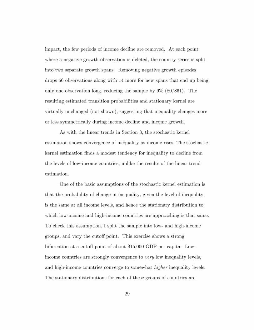
Most of the data (78%) come from 1995 to 2009. Almost all the

data are from 1985 or later (91%), but a few countries have good quality

data earlier than this, in the case of India going back annually to 1951.

The data for Eastern Europe and the former Soviet Union before

1994 are excluded to avoid picking up the sudden inequality changes after

the collapse of central planning. Including these data would strengthen

the apparent convergence of income distributions across countries (since

12

these countries had very low inequality during the Communist era), but

were not included because this historical break was not the result of the

typical process of economic development observed in other countries.

Gini coefficients are paired with income levels in each country and

year. Income levels are measured by gross domestic product (GDP) per

capita from the Penn World Tables version 7.0 (Heston and others, 2011).

The GDP per capita figures are adjusted for purchasing power parity and

reported in 2005 constant international dollars (which are calibrated to

represent the purchasing power of one dollar in the United States in 2005).

3 Linear and Piece-wise Linear Trends

The simplest way to evaluate the path of inequality as income

grows is with a linear trend. Countries may have higher or lower base

levels of inequality for historical reasons or due to differences in

measurement, such as calculating inequality using household consumption

instead of household income. Since we are interested in the typical

pattern of change within countries, we control for different inequality

levels in each country with fixed effects estimation.

The ordinary least squares linear fit of the data in Figure 1 suggests

a dramatic decline of inequality levels as incomes rise. The pattern of

inequality seen in the data could arise even in a world where inequality

never changes in any country, as shown in Figure 2. Fixed effects

13

regression, on the other hand, would correctly estimate that inequality is

not related to income level.

Figure 3 and Table 2 show linear and quadratic fixed effects trend

lines for all the countries. The trend lines in Figure 3 are superimposed on

the individual country data series. The slope of the overall trend is

slightly positive, but not significantly different from zero. It is very

different from the steep decline in inequality suggested by the ordinary

least squares fit in Figure 1.

Table 2: Fixed effects trend lines

Linear trend

Quadratictrend

Above trend

Below trend

GDP per capita ('000 $) 0.042 -0.012 -0.302 0.120 (1.16) (0.13) (2.34)* (2.94)** GDP per capita2 0.001 (0.86) Constant 35.732 36.285 45.749 26.100 (62.66)** (32.18)** (46.31)** (26.81)** R2 0.00 0.01 0.05 0.06 N 865 865 444 421

* p<0.05; ** p<0.01 Robust t statistics in parentheses

The trend in inequality is not significantly curvilinear. The

quadratic trend is virtually indistinguishable from the linear trend and

slightly concave, contrary to the inverted-U shape hypothesized by

Kuznets (1955).

A simple way to check for convergence of inequality across

14

countries is to see if inequality levels are more likely to be falling if the

country starts out above the trend line of inequality and more likely to be

rising if the country starts out below the trend. Figure 3 and Table 2

show the fixed effects trends for higher inequality countries (“above trend”)

and for lower inequality countries (“below trend”).5

The high inequality “above trend” countries show a large and

statistically significant decline in inequality, indicating that high

inequality countries have experienced more reduction in inequality in

recent decades than lower inequality countries.

The low inequality “below trend” countries have a statistically

significant increase in inequality as income grows. If countries start out

above the trend their inequality declines relative to trend, and if they start

out below trend, their inequality increases relative to trend.

The striking pattern in Figure 1 of apparent convergence of

inequality is displayed in terms of the level of GDP per capita. Inequality

is more often compared to the natural logarithm of income than to income

itself, but in this case convergence is not so apparent to the eye. Using

the logarithm of GDP per capita has two advantages. First, if a country

is growing at a constant rate, the income will advance by the same

5 The level of the intercept of the predicted fixed effects trend line is set to pass through the median of the Gini coefficients rather than the mean in Figure 3 (and Figure 4). This causes the groups of countries “above trend” or “below trend” to have approximately equal numbers of observations. The exact level at which the overall trend is set has little effect on the estimated “above trend” and “below trend” coefficients.

15

increment each period on a logarithmic scale. Second, the distribution of

countries by income level is highly skewed so that there are many more

low-income countries than high-income countries. The country data are

more uniformly spaced along a logarithmic scale rather than being

bunched towards the origin.

Figure 4 and Table 3 show the trend of inequality using a

logarithmic scale. The overall trend on the logarithmic scale is slightly

positive and not statistically significant, like the non-logarithmic case.

Similarly, the quadratic term in income is not statistically significant and

the quadratic trend line is almost indistinguishable from the linear trend,

although there is the slightest concavity.

Table 3: Fixed effects trend lines, log GDP

Lineartrend

Quadratic trend

Above trend

Below trend

ln(GDP per capita) 0.233 -2.749 -2.770 5.038 (0.25) (0.36) (2.95)** (3.49)** ln(GDP per capita)2 0.170 (0.41) Constant 34.247 47.139 67.194 -20.416 (3.94)** (1.33) (8.26)** (1.44) R2 0.00 0.00 0.06 0.18 N 865 865 452 413

* p<0.05; ** p<0.01 Robust t statistics in parentheses

There are again clear indications of convergence in inequality in this

16

case. Countries starting out with inequality above the linear trend show a

significant decline in inequality. Below trend countries show an even

steeper, statistically significant, increase in inequality.

The fixed effects estimates imply that for a typical country starting

above the trend level of inequality, when income doubles the Gini

coefficient declines by about 1.9 points.6 A typical country starting below

the inequality trend would tend to see an increase the Gini coefficient of

3.5 points when income per capita doubled.

Do the trends in inequality differ for low-income, middle-income,

and high-income countries? Is there consistent evidence of convergence

throughout the range of income levels? Figure 5 and Table 4 present

three different fixed effects trends according to income level, accompanied

by the trends of “above trend” and “below trend” countries in each income

category.7 The trend lines by income level in Figure 5 are superimposed

on individual country trend lines (rather than the data).

All three of the above trend coefficients are negative and all three

of the below trend coefficients are positive, though not all are statistically

significant. The above trend coefficient in each income level is, however,

statistically significantly different from the below trend coefficient in all

6 A doubling of income is an increase in the log of income of 0.693. Applying the “above trend” coefficient for log GDP per capita, 0.693 * -2.770 = -1.920.

7 Each fixed effects regression includes an intercept which is not reported. The income categories are each 1.6 log GDP per capita wide, with low income ranging from $590 to $2700, middle income from $2700 to $13,400, and high income from $13,400 and above.

17

income categories. The differences between the above and below trend

coefficients are robust to variation in the income level break points (not

shown).

Table 4: Piecewise linear trend lines log GDP per capita coefficients

Low

income Middle income

High income

Above trend -3.700 -6.627 -1.746 (1.91) (3.41)** (0.98) Trend 1.297 -0.979 0.392 (0.52) (0.73) (0.30) Below trend 5.770 1.655 3.764 (1.51) (1.02) (3.44)** Above - Below -9.470 -8.282 -5.510 (2.30)* (3.31)** (2.67)** N 122 357 383

* p<0.05; ** p<0.01 Robust t statistics in parentheses

The robustness of the linear inequality trends is checked in two

ways, first using an independent data sample and second with controls for

possible measurement error.

The Deininger-Squire (1996) dataset provides independent, if error-

prone, estimates of inequality. The statistics cover an earlier period, with

no data in common with the sample otherwise used in this paper. A small

number of country-year pairs overlap in the two data sets, but each of

these data points come from different sources. Few countries overlap in

18

time. The average first year in the Deininger-Squire data is 1972 and the

average final year is 1988, versus an average span from 1991 to 2006 in the

new data.

The Deininger-Squire data exhibit the same pattern of convergence,

but as one might expect from data subject to substantial measurement

error, the levels of significance are a lot lower. Table 5 shows the “above

trend” inequality falling in high inequality countries and the “below trend”

inequality rising in low inequality countries, but neither estimate is

significant at the 5% level. The above trend coefficient is statistically

different from the below trend coefficient at the 14% level.

Table 5: Deininger-Squire fixed effects trend lines

Above Below trend trend

ln(GDP per capita) -1.902 0.677 (1.30) (0.73) Constant 58.304 24.119 (4.82)** (3.07)** R2 0.02 0.01 N 317 289

* p<0.05; ** p<0.01

The new sample, although more consistently measured than the

Deininger-Squire data, is surely still subject to measurement error. If

there is a large bias in the first inequality estimate in each country, and

19

the bias diminishes with each subsequent observation, this could generate

a spurious pattern of inequality convergence. On the other hand

measurement error that is constant over time, or uncorrelated with time,

even if it were high, would not give the appearance of convergence.

The data in this study are all generated from ongoing national

household sample surveys conducted by government statistical offices.

Almost all of the statistical offices have conducted many other surveys

(such as population censuses and price, labor force, and enterprise surveys)

for years before undertaking their first household income or expenditure

survey. If there is a substantial learning curve for conducting a household

economic survey, it is likely to be an issue the first or second time the

national survey is fielded. After that the statistical office has established

its methods and practice. Some level of error inevitably remains, but

there is no compelling reason why it would continue to decline over time.

As a point of comparison, estimating income inequality from household

economic surveys is much simpler than producing national accounts and

GDP estimates, which depend on data from a myriad of different surveys

and reporting mechanisms.

To test for measurement error bias, we repeat the estimation of

above trend and below trend inequality, omitting the first or the first two

inequality observations in each country.8 Table 6 contains the coefficient

8 Regressions using non-logarithmic GDP per capita (not shown) exhibit the

20

estimates for income when the Gini coefficient is regressed on the log of

income and a country-specific constant. When one or two initial

observations are dropped, the results show no qualitatively different

patterns for convergence. Above trend countries still show a statistically

significant decline in inequality and below trend countries still show a

statistically significant increase in inequality. The estimated strength of

the convergence is actually slightly greater when the first two observations

in each country are deleted. The results reject measurement error as a

spurious source of convergence.

Table 6: Measurement error regressions Fixed effects log GDP per capita coefficients

All data W/o first observation

W/o first two observations

Above trend -2.770 -2.365 -3.070 (2.95)** (2.03)* (2.42)*

Trend 0.233 -0.482 -0.532 (0.25) (0.54) (0.55) Below trend 5.038 3.140 5.151

(3.49)** (2.30)* (3.37)** * p<0.05; ** p<0.01

Robust t statistics in parentheses

The individual country trend lines exhibit substantial diversity in

inequality change. Although the cross-country trend lines indicate overall

tendencies, they ignore the churning of inequality levels in different

same patterns.

21

directions at the same income level. The stochastic kernel estimation in

Section 4 will allow us to evaluate the consequences of this

multidirectional churning of the cross-country distribution of inequalities

as income changes.

4 Stochastic Kernel Estimation

The previous section used linear trends in inequality (controlling for

country fixed effects) to make a simple evaluation of the convergence of

inequality as income grows. A fuller assessment would consider the

evolution of the whole distribution of inequalities as income rises, rather

than just the linear trend. A linear trend, for instance, could mask a

dynamic where certain countries tend towards one level of inequality and

other countries tend towards a different level of inequality, even among

high inequality countries. The data show substantial diversity across

countries in the path of inequality whether they start out with high

inequality or low inequality. There are also changes of the direction of

inequality within countries, where falling inequality switches to rising

inequality and vice versa.

Stochastic kernel estimation is flexible enough to model the net

outcome of complex dynamics of inequality change. It can incorporate a

dynamic path where all countries tend towards a single level of inequality

or where they tend towards two or more different levels of inequality. It

can also incorporate a dynamic path where countries switch places

22

between different levels of inequality, while the overall distribution of

cross-national inequalities remains the same.

Stochastic process models are typically applied to processes that

evolve over time. However, most hypotheses about income distribution

concern the path of inequality as income grows, not as time passes. For

this reason, we model the cross-country distribution of inequalities in the

income domain rather than in the time domain. 9

The stochastic kernel model represents the evolution of continuous

distributions from period to period. It is the continuous analogue of a

Markov chain, which represents the evolution of discrete distributions.

Quah (1997, 2007) explains stochastic kernel models and applies them to

the distribution of income levels across countries over time. Since

stochastic kernel models use continuous distribution functions, Quah

defines them using measure theory instead of the more accessible matrix

algebra of Markov chains.

Continuous income distributions are attractive conceptually, but in

practice, stochastic kernel models are estimated by discrete approximation.

Digital computers must approximate continuous transition surfaces with

9 Other estimations of convergence of inequality (Ezcurra and Pascual, 1999, for U.S. states and Kar and others, 2000, for Indian states) specify a stochastic kernel in the time domain rather than the income domain. A stationary distribution in the time domain requires assuming that the transition probabilities are constant over time regardless of what is happening to income. Growth theory often suggests a relationship between inequality and growth (e.g. Banerjee and Newman, 1991) but not predictable changes in inequality over time whether or not there is income growth.

23

discrete grids, so a stochastic kernel model is actually estimated as a fine-

grained Markov chain. Since the model is ultimately estimated using a

discretized distribution, we will present stochastic kernel estimation using

the simpler Markov chain notation. There is no loss of generality since a

continuous distribution can be arbitrarily well approximated by a high

dimension discrete distribution. Refer to Quah (1997, 2007) for the

continuous formulation.

The difference in practice between the stochastic kernel and Markov

chain estimation is the method of calculating the transition matrix.

Markov transition matrices are typically estimated from crude frequency

counts of transitions. Stochastic kernel estimation, in contrast, typically

uses bivariate kernel density.10

The stochastic kernel estimation of the transition matrix can be

finer-grained with more rows and columns because the kernel density

estimation uses information from neighboring cell frequencies to smooth

the density estimates. Whereas a typical Markov transition matrix of

frequencies from a sample of several hundred observations might be a 5x5

matrix to avoid small sample sizes in each transition cell, a bivariate

10 Although stochastic kernel estimation and kernel density estimation both include the term “kernel”, meaning distribution function, they are referring to different uses of a distribution function. Stochastic kernel estimation refers to the estimation of the transition from one period's distribution to the next period's distribution of the variable of interest (here, inequality). Kernel density estimation refers to the weighting scheme for averaging neighboring frequency observations. The weights decline moving away from the cell of interest according to the value of a chosen kernel, or distribution function (e.g. Gaussian, Epanechnikov, rectangular, etc.)

24

kernel density estimator would commonly produce a 50x50 matrix

smoothly approximating the surface.

So in practice a stochastic kernel estimation is a Markov chain

estimated with a smoothed transition matrix.

First divide country inequality into N possible levels, with values

g1,…,gN . The set G = {g1,…,gN} is the state space, and countries move

from one inequality level, gi , to another, gj , at each step of income.

A fundamental assumption of the Markov model is the Markov

property. Let Xs ∈G be the inequality level of a country at income level

s. The Markov property is that assumption that

E Xs+1 X0,…,Xs( )= E Xs+1 Xs( ) . That is, the inequality level at the next

higher income level depends only on the inequality level at the current

income level, and not on the earlier history of inequality levels at lower

income levels. In addition, we assume homogeneity of transitions across

income levels: E Xs+1 Xs( )= E Xs Xs−1( ) for all s. Then we can define the

transition probability as pij = E Xs+1 = gi Xs = gj( ) . The N by N matrix of

all the transition probabilities is P= pij⎡⎣ ⎤⎦ .

Let us be an N-dimensional probability row vector which

represents the state of the Markov chain at income level s. The ith

component of us represents the probability that the chain is at inequality

level gi . Then us+1 = usP . If we assume that for every inequality level gi

25

except for g1 there is a positive probability of inequality falling to gi−1 at

the next income level, and at every inequality level gi except for gN there

is a positive probability of inequality rising to gi+1 at the next income

level, these are sufficient conditions for the Markov chain to be ergodic,

which means there is a possibility of going from every inequality state to

every other inequality state, although not necessarily in one step. By

Doeblin's Theorem (Stroock, 2000, p. 28), ergodic Markov chains tend

towards a unique stationary probability vector as income levels increase

without bound. The stationary probability vector w is defined by

w=s→∞lim u0P

s . w shows us where the distribution of inequalities will end

up if the current distributional dynamic continues indefinitely. The

stationary distribution w is equal to the first left eigenvector of the

transition matrix P, and is independent of the initial distribution u0

(Theorem 8.6, p. 106, Billingsley, 1979).

This Markov model allows for a broad range of inequality dynamics

such as convergence towards single or multi-peaked inequality levels,

divergence, and churning of countries across inequality levels whose overall

dispersion does not change.

Estimating the transition matrix requires some conditioning of the

data. We need to observe the change in inequality across regular income

level intervals. Country inequality levels are measured at regular time

intervals (every year in countries with an annual income survey), not at

26

regular income intervals. To construct a progression of inequality over

equally spaced log income intervals, income is quantized into 200 equal log

income levels. If more than one sequential inequality observation falls

within a given income interval (when income grows too little to progress

to the next income level), the inequality observations are averaged.

The categorization of the data into regular income levels produces

an inequality “income series” (as opposed to a time series) with a lot of

gaps, especially in countries with rapid economic growth, because income

may jump several levels between inequality observations. These gaps are

bridged by linear interpolation of between income levels in a given country

to maintain a connected series (just as a country’s observations are

typically connected by straight lines in graphs, as in Figure 1). To

prevent rapidly growing countries with more interpolated observations

having disproportionate influence, the observations are weighted by the

number of actual, non-interpolated, data points when estimating the

transition matrix.

The regridding of inequality takes the original 861 observations and

interpolates them up to 2,035 inequality transition observations.

The transition matrix P is estimated from a bivariate kernel

density, using a Gaussian kernel with a bandwidth of 2.5. The estimation

generates a 50 by 50 transition matrix which smooths the raw transition

matrix frequencies. The transitions are from the level of the Gini

coefficient at the current income level to the level of the Gini coefficient at

27

the next income level.

The density contours of transition matrix estimated from the

sample are graphed in Figure 6. There is a unique peak at point A (a

Gini coefficient of 31.5), indicating convergence of inequality levels toward

a single peak of attraction.

To the left of point A, the probability mass of the transition matrix

is distended to the west, and to the right of point A, the probability mass

is distended to the east, drawing inequality levels to the point of

attraction at A. For inequality at income level s on the horizontal axis,

consider starting at a Gini coefficient of 22. The density of the transition

probabilities is heavily weighted towards higher inequality at income level

s+1. The density mass for the current Gini of 22 is predominantly above

the 45° line, meaning that inequality is more likely to rise than fall next

income level. In contrast, the density of inequalities next income level

starting at a Gini of 38 is mostly below the 45° line, showing that

inequality is most likely to fall next period. These tendencies in the

transition matrix draw inequalities towards point A as income grows.

The transition matrix P shown in Figure 6 has a stationary

inequality distribution w . Figure 7 displays the stationary kernel along

with the distribution of inequalities for low-income countries with income

per capita below $10,000, and the distribution for high-income countries

with income per capita above $20,000. The stationary kernel is more

compact than the low-income distribution, but less compact than the high-

28

income distribution.

The dotted lines indicate the mean inequality for each distribution.

The mean inequality of the stationary kernel, at 35.6, is significantly

smaller than the mean inequality of low income countries, at 42.3, and

significantly larger than the inequality of high income countries, at 29.2.11

The shape and location of the stationary kernel are robust to the

choice of kernel and bandwidth. The stationary kernel has a very similar

shape using either an Epanechnikov or a rectangular kernel (the latter

being about as different from a Gaussian as one can get), although since

these kernels limit the range of smoothing, a smoothness similar to the

Gaussian kernel requires a higher bandwidth. All three kernels result in a

somewhat more compact stationary distribution with a lower mean

inequality at lower bandwidths and a more spread out stationary

distribution with a higher mean inequality at high bandwidths. A

Gaussian kernel with a bandwidth of 0.2 produces a stationary

distribution with a mean inequality of 34.3 and a bandwidth of 5 produces

a mean inequality of 36.1, compared to a mean of 35.6 with a bandwidth

of 2.5. Bandwidths below the chosen level of 2.5 cause local jaggedness in

the stationary distribution.

It is possible that inequality change during periods of income

decline is different from changes when income grows. To evaluate its

11 We can use an ordinary t test, since the stationary distribution w is independent of the initial

distribution u0 . The means are different at the 1% level.

29

impact, the few periods of income decline are removed. At each point

where a negative growth observation is deleted, the country series is split

into two separate growth spans. Removing negative growth episodes

drops 66 observations along with 14 more for new spans that end up being

only one observation long, reducing the sample by 9% (80/861). The

resulting estimated transition probabilities and stationary kernel are

virtually unchanged (not shown), suggesting that inequality changes more

or less symmetrically during income decline and income growth.

As with the linear trends in Section 3, the stochastic kernel

estimation shows convergence of inequality as income rises. The stochastic

kernel estimation finds a modest tendency for inequality to decline from

the levels of low-income countries, unlike the results of the linear trend

estimation.

One of the basic assumptions of the stochastic kernel estimation is

that the probability of change in inequality, given the level of inequality,

is the same at all income levels, and hence the stationary distribution to

which low-income and high-income countries are approaching is that same.

To check this assumption, I split the sample into low- and high-income

groups, and vary the cutoff point. This exercise shows a strong

bifurcation at a cutoff point of about $15,000 GDP per capita. Low-

income countries are strongly convergence to very low inequality levels,

and high-income countries converge to somewhat higher inequality levels.

The stationary distributions for each of these groups of countries are

30

graphed in Figure 8. The stationary distribution of inequality for

countries with GDP per capita below $15,000 has a mean of 27.1,

significantly below even the mean of current high-income countries, and

the stationary inequality distribution is tightly bunched near the mean.

The means that the transition dynamic is leading all low-income countries

towards very low inequality, with little difference between the countries.

The stationary distribution for high-income countries has a higher

mean of 32.1 and is more spread out than the stationary distribution for

low-income countries.

The shape of the stationary distribution for low-income countries is

virtually unchanged if the cut-off for low income is set at $10,000 or at

$5,000, but the tendency to converge to low inequality levels diminishes as

the cut-off rises above $15,000. For high income countries, the stationary

distribution loses its tendency to convergence towards higher inequality at

cut-offs below $12,000 or above $18,000.

The results suggest two convergence dynamics, or at least

convergence intensities, a powerful one for low-income countries towards

very low inequality (even though many low-income countries currently

have quite high inequality) and a weaker convergence for high-income

countries towards slightly higher inequality than they currently have. The

high-income countries are nonetheless converging towards a lower

inequality than the current average across all countries.

31

5 Some country and regional inequality trends It is a common perception, if unsupported by data, that inequality

is worsening around the world. Much of that perception comes from the

recent experience of the United and China, the biggest countries in the

world in terms of economic size and population, respectively. Both

countries have seen a dramatically worsening of inequality in recent

decades, but they are uncharacteristic of most of the rest of the countries

in the world. It is useful to compare the inequality change in these

countries with others.

The U.S. has had rapidly worsening inequality since the late 1970s

(Piketty and Saez, 2003, Gottschalk and Danziger, 2003). Many other

high-income countries have also experienced modestly increasing inequality

over this period, especially in the past decade, but the speed of increase is

highest in the U.S.12, and its level of inequality is now is much higher than

other high-income countries. Figure 10 shows the inequality paths of

high-income countries including the U.S. The trend line is the fixed

effects trend for countries with GDP per capita above $25,000. The U.S.

is now the only high-income OECD country with inequality above the

world average.

China, two-fifths of the world's population, has had the fastest

12 The speed of increase in the United Kingdom may have been as high or higher than the U.S. in the 1980s, but the U.K. started from a much lower level of inequality. Atkinson (1997) estimates that between 1978 and 1992, the Gini coefficient rose more than 10 points, bringing the U.K. from one of the lower inequality levels in Western Europe to the highest.

32

economic growth of any country from 1980 until 2009, which is probably

the fastest sustained economic growth in history13. China has also had the

largest rise in inequality of any country in the sample, rising from a Gini

coefficient of 22.4 in 1985 to 44.9 in 2003. This increase is 10 points

higher than the next highest increase in the sample (Armenia) and more

than twice as high as the third highest increase.

Is China's extraordinary rise in inequality the result of its rapid

economic growth? This question is beyond the scope of this paper, but a

good point of comparison is Vietnam. Since implementing market

liberalization about 1990, Vietnam has been the fifth fastest-growing

economy in the world.14 It is among the larger nations of the world, with

the 13th largest population, and it emerged from centrally planning a

decade after China, with a similar path of market-oriented reforms.

Vietnamese inequality rose in the first decade after reforms, but inequality

has not risen since. Although almost all countries transitioning from

central planning initially see increases in inequality (as in Eastern Europe

and the former Soviet Union), Vietnam's recent experience suggests that

China's continuing rise in inequality is not the inevitable consequence of

13 This is ignoring Equatorial Guinea, a tiny country that discovered oil. The growth rates are calculated from the Penn World Tables 7.0 (Heston et al., 2011), using real GDP per capita (rgdpch). China's income level grew at 8.9% or 7.4% per year from 1980 to 2009 depending on which of the two Penn World Table estimates of China's GDP one uses.

14 Vietnam's GDP per capita grew at 5.9% from 1990 to 2009 in the manner explained in the previous footnote, behind Equatorial Guinea, China, Bosnia and Herzegovina, and Trinidad and Tobago.

33

rapid economic growth or market liberalization.

The rapid rise in inequality in recent decades has made the U.S. the

great outlier of developed countries and China the outlier among

developing countries. Their inequality rise is much faster than would be

predicted by convergence of low-inequality countries. There is no evidence

that within-country inequality is increasing in the world as a whole.

The convergence of inequality is consistent with two recent regional

trends. Latin American countries have some of the highest inequality

levels in the world, and have experienced some of the fastest declines in

inequality in the past couple of decades. The highest income countries,

which have some of the lowest inequality levels in the world, have

experienced increasing inequality in recent decades. Both these trends are

shown in Figure 11 and Table 7.

Table 7: Regional fixed effects trend lines High GDP

OECDa

Latin America

E. Europe & FSU

Emerging Asia

b Low &

Mid GDPc

ln(GDP p.c.) 4.625 -6.661 -0.532 3.713 -0.309 (2.95)** (2.11)* (0.32) (2.47)* (0.28) Constant -19.759 108.042 37.503 8.575 41.790 (1.21) (3.89)** (2.49)* (0.70) (4.36)** R2 0.12 0.12 0.00 0.15 0.00 N 223 213 193 69 628

Robust t statistics in parentheses a High GDP OECD includes OECD90 countries with GDP per capita above $25,000.

b Emerging Asia includes Asian countries with GDP per capita between $1,500 and $10,000.

c Low & Mid GDP are all countries with GDP per capita below $25,000.

Three other regions have a mixture of below- and above-average

34

inequality levels. Eastern Europe and the former Soviet Union countries

as a whole show no significant trend inequality (since 1994 by which time

inequality in many of the countries had risen significantly from levels

under central planning). “Emerging Asia” is made up of Asian countries

with GDP per capita between $1,500 and $10,000. Two thirds of

countries15 in this group have rising inequality in the data, and the region

as a whole has a significant rise in inequality. Finally, all the low- and

middle-income countries (with GDP per capita below $25,000) show a

slight, but insignificant, decline in inequality.

6 Conclusion This study is the first to test for convergence of inequality using

internally consistent time series of inequality for a large number of

countries. The data show strong evidence of convergence. High inequality

countries have seen their inequality levels fall, on average, as income rose

in recent decades, and low inequality countries have seen their inequality

levels rise on average. Using three different methods, linear trends,

piecewise linear trends, and stochastic kernel estimation, the typical trend

in less equal countries was the opposite of the trend in more equal

countries, pushing inequality levels in both groups towards each other.

15 China, Indonesia, Iran, Sri Lanka, the Philippines, Thailand, Taiwan, and Vietnam all have

rising inequality trends in the sample, and Jordan, Malaysia, Pakistan, and Turkey have falling inequality trends. Asia as a whole has a rising, but statistically insignificant trend.

35

The evidence for inequality convergence is consistent with the

apparent narrowing of inequality as income rises in Figure 1. However,

the dramatically falling trend in average inequality in Figure 1 is not so

clear once one accounts for differences in country inequality levels. There

is no clear trend of inequality within countries in the linear analysis. The

stochastic kernel estimation shows lower income countries tending towards

dramatically lower inequality levels in the stationary state, and higher

income countries tending towards a modestly higher inequality. It is not

clear why the linear and stochastic kernel results for overall inequality

trends are different. The stochastic kernel estimation predicts that the

Gini coefficient of countries with GDP per capita below $15,000 is

predicted to fall from a current average if 41.3 to an average of 27.1 in the

stationary state. The Gini coefficient of countries with GDP per capita

above $15,000 is predicted to rise from an average of 29.5 currently to an

average of 32.1 in the stationary state.

The patterns found in this new inequality data could be viewed

good or bad news. The good news is that there is no sign of a tendency

for low-income countries as a group to experience worsening inequality as

their economy grows, unlike Kuznets's prediction. High inequality

countries in particular, whether lower income or higher income, have

tended to see substantial declines in inequality with economic growth.

There also evidence using stochastic kernel estimation for a decline in

inequality for all low income countries as they approach higher income

36

levels.

The bad news is that countries with unusually low inequality tend

to see increases in inequality. The recent increases in inequality in higher

income countries fit this trend of rising inequality.

One can speculate about possible reasons for a convergence of

inequality with economic growth. First, trade and other forces of

globalization may cause the income earned by different segments of society

to become more similar across countries as income grows. The share of

trade and other links to the outside world tend to grow with income levels.

The convergence of inequality due to trade may be evidence of factor price

equalization predicted by the Hecksher-Ohlin trade model (see Deardorff,

2001, for example).

Second, democratic participation tends to increase with income

levels, and greater political activism by lower income citizens could change

the income distribution through government tax rates and transfers, as

well as union rights, government funding for education and health and

other policies. Political pressure for policies that reduce income inequality

is more likely to be strongest in countries that start out with higher

inequality, leading to convergence.

A third possible cause of convergence comes from growth models

with credit constraints, as noted by Bénabou in the introduction. The

credit constraints cause inequality due to the asymmetric advantages in

saving and investment of the initially unconstrained higher income

37

households. As income levels rise, fewer and fewer households remain

constrained. The role of inequality in theoretical models of growth is

surveyed in Bertola, et al. (2005).

A fourth dynamic by which economic growth could lead to

inequality convergence is diversity in land ownership concentration across

countries. Countries with more unequal ownership of agricultural land

would have higher inequality of farm incomes. Since the share of

agriculture diminishes in the economy as it grows, the role of land

ownership in inequality would diminish, pushing countries towards more

similar inequality levels. One would expect this dynamic to be most

important at low income levels when agriculture is a large share of GDP,

but in the data, inequality convergence is also clear in middle- and high-

income countries as well.

A challenge for empirical research on inequality is that everything

that influences incomes (employment, capital markets, education, trade,

social welfare programs, savings, etc., etc.) also affects income distribution.

This makes it difficult to isolate the specific causes of inequality

convergence, just as empirical research on the causes of economic growth

is difficult because almost everything affects GDP levels.

The convergence of inequality is in stark contrast to the general

lack of convergence of income levels across countries. The convergence of

inequality occurs when there is income growth, so if low-income countries

fail to grow economically they would not be exposed to this tendency.

38

The convergence of inequality will do little to improve the world

distribution of income if the poorest countries are growing the slowest.

However, if a poor country with high inequality is able to grow

economically, there is a good chance that inequality will also fall.

PORTLAND STATE UNIVERSITY

1

References

[1] Atkinson, Anthony Barnes, and Andrea Brandolini. 2001. “Promise

and Pitfalls in the Use of 'Secondary' Data-Sets: Income Inequality in

OECD Countries as a Case Study,” Journal of Economic Literature 39:

771-99.

[2] Atkinson, Anthony B., Thomas Piketty, and Emanuel Saez. 2011.

“Top Incomes in the Long Run of History,” Journal of Economic

Literature 49(1):3-71.

[3] Ayagari, R. 1994. “Uninsured idiosyncratic risk and aggregate savings,”

Quarterly Journal of Economics 109:659-684.

[4] Banerjee, Abhijit V., and Esther Duflo. 2003. “Inequality and Growth:

What Can the Data Say?” Journal of Economic Growth 8:267-299.

[5] Banerjee, A., and A. Newman. 1991. “Risk-bearing and the theory of

income distribution,” Review of Economic Studies 58:211-236.

[6] Bénabou, Roland. 1996. “Inequality and Growth,” in Bernanke, Ben S.,

and Julio J. Rotemberg, eds., NBER Macroeconomics Annual 1996,

Volume 11. Cambridge, MA: MIT Press.

[7] Bertola, Giuseppe. 1995. “Accumulation and the extent of inequality,”

London, England: Centre for Economic Policy Research Discussion

Paper 1187.

[8] Bertola, Giuseppe, Reto Foellmi, and Josef Zweimüller. 2005. Income

2

Distribution in Macroeconomic Models. Princeton, New Jersey:

Princeton University Press.

[9] Billingsley, Patrick. 1997. Probability and Measure. New York: Wiley

and Sons.

[10] Cowell, Frank A. 2008. Measuring Inequality.

http://darp.lse.ac.uk/papersDB/Cowell_measuringinequality3.pdf,

accessed September 12, 2009.

[11] Coulter, Fiona A. E., Frank A. Cowell, and Stephen P. Jenkins. 1992.

“Equivalence Scale Relativities and the Extent of Inequality and

Poverty,” Economic Journal 102(September):1067-82.

[12] Deardorff, Alan V. 2001. “Does Growth Encourage Factor Price

Equalization?” Review of Development Economics, 5(2):169-81.

[13] Deininger, Klaus, and Lyn Squire. 1996. “A New Data Set Measuring

Income Inequality,” World Bank Economic Review 10(3): 565-91.

[14] Eurostat. 2011. “Gini coefficient (Source: SILC) (ilc_di12).” Accessed

2/17/2011 from

http://epp.eurostat.ec.europa.eu/portal/page/portal/statistics/search_

database.

[15] Ezcurra, Roberto, and Pedro Pascual. 2009. “Convergence in income

inequality in the United States: a nonparametric analysis,” Applied

Economics Letters 16:1365–1368.

3

[16] Gallup, John Luke. 2012. “Is There a Kuznets Curve?” unpublished.

[17] Heston, Alan, Robert Summers, and Bettina Aten. 2011. Penn World

Table Version 7.0, Center for International Comparisons of Production,

Income and Prices at the University of Pennsylvania, May 2011.

[18] Jenkins, Stephen P., and Frank A. Cowell. 1994. “Parametric

Equivalence Scales and Scale Relativities.” Economic Journal

104(July):891-900.

[19] Kar, Sabyasachi, Debajit Jha, and Alpana Kateja. 2010. “Club-

Convergence and Polarisation of States: A Nonparametric Analysis of

Post-Reform India,” Delhi: Institute of Economic Growth working

paper 307.

[20] Kuznets, Simon. 1955. “Economic Growth and Income Inequality,”

American Economic Review 45(1):1-28.

[21] Lin, Pei-Chien and Ho-Chuan (River) Huang. 2009. “Inequality

convergence in a panel of states,” Journal of Economic Inequality 9:195–

206.

[22] LIS. 2011. “Luxembourg Income Study Database: Inequality &

Poverty – Key Figures – All Waves.” Accessed 8/5/2011 from

http://www.lisdatacenter.org/data-access/key-figures/download-key-

figures/.

[23] Panizza, Ugo. 2001. “Convergence in Income Inequality,” Journal of

4

Income Distribution 10(1-2):5-12.

[24] Piketty, Thomas. 1997. “The dynamics of the wealth distribution and

interest rate with credit-rationing,” Review of Economic Studies

64(2):173-189.

[25] Quah, Danny T. 1993a. “Empirical cross-section dynamics in economic

growth,” European Economic Review 37:426-434.

[26] Quah, Danny T. 1993b. “Galton's Fallacy and Tests of the

Convergence Hypothesis,” The Scandinavian Journal of Economics

95(4):427-443.

[27] Quah, Danny T. 1997. “Empirics for Growth and Distribution:

Stratification, Polarization, and Convergence Clubs,” Journal of

Economic Growth 2:27–59.

[28] Quah, Danny. 2007. Growth and Distribution. Book draft accessed

August 25, 2011 from http://econ.lse.ac.uk/staff/dquah/.

[29] Ravallion, Martin. 2003. “Inequality convergence,” Economics Letters

80:351–356.

[30] SEDLAC. 2011. “Socio-Economic Database for Latin America and the

Caribbean (CEDLAS and The World Bank), July 2011 version - 13.

Accessed 8/5/2011, http://sedlac.econo.unlp.edu.ar/eng/statistics.php.

[31] Stroock, Daniel W. 2000. An Introduction to Markov Chains. Berlin:

Springer.

5

[32] TransMONEE. 2011. “The TransMONEE Database, 2011 version.”

Accessed 2/16/2011 from http://www.transmonee.org/.

[33] WIID. 2008. “UNU-WIDER World Income Inequality Database, Version 2.0c, May 2008.” Accessed 1/14/2011 from http://www.wider.unu.edu/research/Database/en_GB/database/.

37

Figure 1: Inequality Versus Income Series for 87 Countries

2030

4050

60G

ini c

oeffi

cien

t

0 10,000 20,000 30,000 40,000 50,000GDP per capita (PPP)

OECD90Latin AmericaE. Europe & FSUAfricaAsiaOLS fit (t = 20.4)Quadratic fit

Figure 2: Spuriously estimated inequality decline

2030

4050

Gin

i coe

ffici

ent

0 10000 20000 30000 40000 50000GDP per capita

Country time seriesOLS fit

38

Figure 3: Linear and quadratic fixed effect inequality trends

2030

4050

60G

ini c

oeff

icie

nt

0 10,000 20,000 30,000 40,000GDP per capita (PPP)

Above trendTrendBelow trendQuadratic trend

Figure 4: Linear and quadratic inequality trends on a logarithmic scale

020

4060

80G

ini c

oeff

icie

nt

1,000 2,000 4,000 8,000 16,000 32,000GDP per capita (PPP)

Above trendTrendBelow trendQuadratic trend

39

Figure 5: Low, middle, and high income linear trends on a log scale

2030

4050

60

1000 2000 4000 8000 16000 32000 64000600 2700 13000

GDP per capita (PPP)

Above trendTrendBelow trend

Figure 6: Bivariate kernel density estimates of transition matrix

A

2030

4050

60Gini s+1

22 3820 30 40 50 60Ginis

40

Figure 7: Stationary kernel with low and high income inequality

Stationarykernel

GDP p.c.> $20,000

GDP p.c.<= $10,000

0.00

0.02

0.04

0.06

0.08

0.10

Den

sity

20 25 30 35 40 45 50 55 6029.2 35.6 42.3

Gini coefficient

Figure 8: Stationary kernels below and above $15,000 GDP p.c.

GDP p.c.> $15_,000

GDP p.c.<= $15,000

Stationarykernel

> $15,000

Stationarykernel

<= $15,000

0.00

0.02

0.04

0.06

0.08

0.10

Den

sity

20 25 35 40 45 50 55 60 6527.129.5

32.141.3

Gini coefficient

41

Figure 9: U.S. and high-income OECD inequality trends

1974

1979

1997 2004USA

High-incometrend

World average Gini = 36.4

20

25

30

35

40

Gin

i coe

ffic

ient

25000 30000 35000 40000GDP per capita

Figure 10: China and low-income inequality trends

1985

1995

2003

1993

2002

2008

Avg.low-incomeGini = 40.1

20

30

40

50

60

Gin

i coe

ffic

ient

500 1000 1500 2000 2500 3000 3500 4000 4500GDP per capita

Latin America E. Europe & FSU AfricaAsia China Vietnam

42

Figure 11: Regional fixed effects inequality trends

20

30

40

50

60

Gin

i coe

ffici

ent

1500 10000 250001000 2000 4000 8000 16000 32000 64000

GDP per capita (PPP)

High GDP OECDa

Latin AmericaE. Europe & FSUEmerging Asiab

Low & Mid GDPc

a “High GDP OECD” includes OECD90 countries with a GDP per capita above $25,000 b “Emerging Asia” includes Asian countries with GDP per capita levels between $1,500 and $10,000. c Low & Mid GDP are all countries with GDP per capita below $25,000.

1

Online Data Appendix

This appendix lists the sources and definitions used for each of the countries in the sample. Table A.1 shows the sources of inequality data along with the income concept used and the within-household weights applied.

Table A.1. Sources of Gini coefficients

Source

No. of countries

Income concept

Household weights*

Eurostat 21 Disposable Income Equivalent 1

TransMONEE 19 Disposable Income Per capita

SEDLAC 18 Disposable Income Equivalent 2

LIS 4 Disposable Income Per capita

WIID 22 Varied Varied

Other 3

Canada Disposable Income Equivalent 3

Indonesia Consumption Per capita

Vietnam Consumption Equivalent 1

Total 87 * Equivalent 1 = Modified OECD adult equivalent weights; Equivalent 2 = Household equivalent D (from SEDLAC, 2011);

Equivalent 3 = Square root of family size. See online data appendix for details. Household equivalency scales

The Gini coefficients are calculated with equivalized household income obtained by dividing total household income by factors which differ according to the equivalency scale. Equivalency scales capture the sensible idea that there are economies of scale in household consumption, but there is no generally accepted equivalency scale, and Deaton (1992)

2

argues that it is not possible to estimate household equivalency scales because they inherently unidentifiable. In the Table A.2, the equivalency scales depend on:

H - household head (the first adult) A - number of other adults (including children aged 14 and over) K1 - number of children aged 5 or younger K2 - number of children between age 6 and 13 years (inclusive)

Table A.2: Equivalency Scales

Household equivalency scale Weights Total Household H Household per capita H + A + K1 + K2 Household eq, OECDmod (OECD, 2005) H + 0.5A + 0.3(K1 + K2) Household eq, D (SEDLAC, 2010) (H + A+ 0.3K1 + 0.5K2)0.75 Household eq, square root (H + A+ K1 + K2)0.5

Household eq, D was chosen because it is the SEDLAC scale closest to the OECD modified scale for typical family

sizes. Income Definitions

Disposable Income after tax household income. There are some differences across countries in the measurement of in kind income, profits, rents, capital income, government transfers, implicit rent from home ownership, etc.

Gross Income Same as disposable income, except it includes taxes. Consumption Household expenditure, generally excluding expenditure on durables.

Sources Sources are citations to the references, except when they are prefixed by “WIID”, in which case they refer to the source referenced in WIID (2008).

3

Table A.3: Sources, definitions, and year coverage by country

Country Years Equivalency scale Income Definition Source Western Europe (Eurostat) Austria 1995-2001, 2003-2009 Household eq, OECDmod Disposable Income WIID:European Commission; Eurostat 2011 (2001-2009) Belgium 1995-2001, 2003-2009 Household eq, OECDmod Disposable Income WIID:European Commission; Eurostat 2011 (2001-2009) Croatia 2002-2008 Household eq, OECDmod Disposable Income Eurostat 2011 Cyprus 2003, 2005-2009 Household eq, OECDmod Disposable Income WIID:European Commission; Eurostat 2011 (2001-2009) Germany 1995-2009 Household eq, OECDmod Disposable Income WIID:European Commission; Eurostat 2011 (2001-2009) Denmark 95,97,99,01,03-09 Household eq, OECDmod Disposable Income WIID:European Commission; Eurostat 2011 (2001-2009) Spain 1995-2002, 2004-2009 Household eq, OECDmod Disposable Income WIID:European Commission; Eurostat 2011 (2001-2009) Finland 1966-2009 Household eq, OECDmod Disposable Income WIID:European Commission; Eurostat 2011 (2001-2009) France 1995-2009 Household eq, OECDmod Disposable Income WIID:European Commission; Eurostat 2011 (2001-2009) United Kingdom 1995-2003, 2005-2009 Household eq, OECDmod Disposable Income WIID:European Commission; Eurostat 2011 (2001-2009) Greece 1995-2001, 2003-2009 Household eq, OECDmod Disposable Income WIID:European Commission; Eurostat 2011 (2001-2009) Ireland 1995-2001, 2003-2009 Household eq, OECDmod Disposable Income WIID:European Commission; Eurostat 2011 (2001-2009) Iceland 2004-2009 Household eq, OECDmod Disposable Income Eurostat 2011 Italy 1995-2001, 2004-2009 Household eq, OECDmod Disposable Income WIID:European Commission; Eurostat 2011 (2001-2009) Luxembourg 1995-2001, 2003-2009 Household eq, OECDmod Disposable Income WIID:European Commission; Eurostat 2011 (2001-2009) Malta 2000, 2005-2009 Household eq, OECDmod Disposable Income Eurostat 2011 Netherlands 1995-2003, 2005-2009 Household eq, OECDmod Disposable Income WIID:European Commission; Eurostat 2011 (2001-2009) Norway 2003-2009 Household eq, OECDmod Disposable Income Eurostat 2011 Portugal 1995-2001, 2004-2009 Household eq, OECDmod Disposable Income WIID:European Commission; Eurostat 2011 (2001-2009) Sweden 1999, 2001-2, 2004-9 Household eq, OECDmod Disposable Income Eurostat 2011 Turkey 2002-2003 Household eq, OECDmod Disposable Income Eurostat 2011 Eastern Europe and the former Soviet Union (TransMONEE) Armenia 1996, 2002-2008 Household per capita Disposable Income Transmonee 2010 Bulgaria 1994-2008 Household per capita Disposable Income Transmonee 2010 Belarus 1995-2008 Household per capita Disposable Income Transmonee 2010 Czech Republic 1994-2007 Household per capita Disposable Income Transmonee 2010 Estonia 1995-2005 Household per capita Disposable Income Transmonee 2010 Georgia 1998, 2001,2002 Household per capita Disposable Income Transmonee 2010 Hungary 1994-2007 Household per capita Disposable Income Transmonee 2010 Kyrgyz Republic 1997-2008 Household per capita Disposable Income Transmonee 2010 Latvia 1994-2004 Household per capita Disposable Income Transmonee 2010 Lithuania 1997-2004 Household per capita Disposable Income Transmonee 2010 Moldova 1997, 2000-2008 Household per capita Disposable Income Transmonee 2010 Macedonia, FYR 1994-2008 Household per capita Disposable Income Transmonee 2010

4

Country Years Equivalency scale Income Definition Source Poland 1994-2008 Household per capita Disposable Income Transmonee 2010 Romania 1994-2008 Household per capita Disposable Income Transmonee 2010 Russia 1994-1996, 1998, 2000, 2001 Household per capita Disposable Income Transmonee 2010 Serbia 2003-2008 Household per capita Disposable Income Transmonee 2010 Slovak Republic 1996-2008 Household per capita Disposable Income Transmonee 2010 Slovenia 1994-2003, 2005 Household per capita Disposable Income Transmonee 2010 Ukraine 1995, 1998-2002, 2007-2008 Household per capita Disposable Income Transmonee 2010 Latin America and Caribbean (SEDLAC) Belize 93,94,97-99 Household eq, D Gross Income SEDLAC, 2011 Bolivia 97,99,01,02,05-07 Household eq, D Gross Income SEDLAC, 2011 Brazil 81-90,93,95-99,01-09 Household eq, D Gross Income SEDLAC, 2011 Chile 87,90,92,94,96,98,00,03,06,09 Household eq, D Gross Income SEDLAC, 2011 Colombia 96,99-01,03,04,06 Household eq, D Gross Income SEDLAC, 2011 Costa Rica 1989-2009 Household eq, D Gross Income SEDLAC, 2011

Dominican Republic 1996-97,2000-08 Household eq, D Gross Income SEDLAC, 2011

Ecuador 95,98,99,03-09 Household eq, D Gross Income SEDLAC, 2011 El Salvador 91,95-96,98-08 Household eq, D Gross Income SEDLAC, 2011 Guatemala 2002-04 Household eq, D Gross Income SEDLAC, 2011 Honduras 1991-99,2001-05,07,09 Household eq, D Gross Income SEDLAC, 2011 Jamaica 90-96,99,01-02 Household eq, D Gross Income SEDLAC, 2011 Mexico 89,92,94,96,98,00,02,04-06,08 Household eq, D Gross Income SEDLAC, 2011 Nicaragua 93,98,01,05 Household eq, D Gross Income SEDLAC, 2011 Panama 89,91,95,97-98,01-06,09 Household eq, D Gross Income SEDLAC, 2011 Paraguay 95,97,99,01-09 Household eq, D Gross Income SEDLAC, 2011 Peru 1997-2009 Household eq, D Gross Income SEDLAC, 2011 Uruguay 2006-09 Household eq, D Gross Income SEDLAC, 2011 Venezuela 89,92,95,98-2006 Household eq, D Gross Income SEDLAC, 2011 Luxembourg Income Study and others Switzerland 82,92,00,02,04 Household per capita Disposable Income LIS, 2011 Unites States 74, 79, 86, 91, 94, 97, 00, 04 Household per capita Disposable Income LIS, 2011 Israel 79, 86, 92, 97, 01, 05 Household per capita Disposable Income LIS, 2011 Taiwan 81, 86, 91, 95, 97, 00, 05 Household per capita Disposable Income LIS, 2011 Canada 1976-2004 Household eq, square root Disposable Income Heinz 2007, Table A.4 (p. 55) Indonesia 76,78,80,81,84,87,90,93,96,99,02-09 Household per capita Consumption WIID: Statistics Indonesia; Statistics Indonesia, 2011 (1999-2009)

5

Country Years Equivalency scale Income Definition Source Vietnam 93, 98, 02, 04, 06, 08 Household eq, OECDmod Consumption author's calculations WIID Albania 2002, 2004 Household per capita Consumption WIID: WB Living Standard Measurement Surveys Australia 81, 85, 89, 95-98, 00-03, 05 Household eq, OECDmod Disposable Income WIID: Australian Bureau of Statistics 2005; Australian Bureau of

Statistics, 2009 (Table S6, p. 11, for 2003 & 2005) Bahamas 73,75,77,79,86,88,89,91-93,03,04 Total household Gross Income WIID: Bahamas Dept. of Statistics, Household Sample Survey Bangladesh 83, 86, 88, 92, 96, 00, 05 Household per capita Consumption WIID: Bangladesh Household Expenditure Survey Botswana 1986, 1994 Household per capita Consumption WIID: Botswana CSO, Household Income and Expenditure Survey Cambodia 1994, 1997, 1999, 2004 Household per capita Consumption WIID: Cambodia Socio-Economic Survey China 85, 91, 95, 00, 03 Household per capita Disposable Income WIID: Chotikapanich et al 2005: Rural/Urban Household Survey India 1951-1992, 2004 Household per capita Consumption WIID: Datt, 1995 & WDI 2004 Japan 1962-1982, 1985, 1990 Total household Disposable Income WIID: Mizoguchi and Takayama 1984; Oshima 1994 Jordan 1992, 1997, 2003 Household per capita Consumption WIID: World Bank South Korea 1992, 1993, 1995-1998 Household eq, square root Disposable Income WIID: Cheong 2005 Laos 1992, 1997, 2002 Household per capita Consumption WIID: World Bank Lesotho 1986, 1993 Household per capita Consumption WIID: World Bank Malaysia 1984, 1987, 1989, 1992, 1995, 1997 Household per capita Gross Income WIID: Household Income Survey Mauritius 1991, 1996, 2001 Total household Disposable Income WIID: Mauritius CSO Morocco 1985, 1991, 1999 Household per capita Consumption WIID: World Bank New Zealand 86, 89, 92, 95, 98, 01, 04 Household eq, square root Disposable Income WIID: Perry 2005 Pakistan 87, 91, 93, 96, 02, 05 Household per capita Consumption WIID: World Bank Philippines 85, 88, 91, 94, 97, 00, 03 Household per capita Consumption WIID: World Bank Sri Lanka 1986, 2000, 2002 Household per capita Consumption WIID: World Bank Thailand 81, 86, 88, 90, 92, 94, 96, 98, 99 Household per capita Consumption WIID: Thailand Socio-Economic Survey Tunisia 1985, 1990, 2000 Household per capita Consumption WIID: World Bank

6

References [1] Australian Bureau of Statistics. 2009. “6523.0 - Household Income and Income Distribution, Australia, 2007-08.” 20/08/2009

Issue. http://www.abs.gov.au/ausstats/abs@.nsf/mf/6523.0, accessed February 21, 2011.

[2] Deaton, Angus S. 1992. Understanding Consumption. Oxford: Clarendon Press.

[3] Eurostat. 2011. “Gini coefficient (Source: SILC) (ilc_di12).” Accessed 2/17/2011 from http://epp.eurostat.ec.europa.eu/portal/page/portal/statistics/search_database.

[4] Heinz, Andrew. 2007. “Income Inequality and Redistribution in Canada: 1976 to 2004.” Ottawa: Statistics Canada Research Paper 11F0019 – 298.

[5] LIS. 2011. “Luxembourg Income Study Database: Inequality & Poverty – Key Figures – All Waves.” Accessed 8/5/2011 from http://www.lisdatacenter.org/data-access/key-figures/download-key-figures/.

[6] OECD. 2005. “What are equivalence scales?” September 27, 2005. Accessed from http://www.oecd.org/dataoecd/61/52/35411111.pdf.

[7] SEDLAC. 2011. “Socio-Economic Database for Latin America and the Caribbean (CEDLAS and The World Bank), July 2011 version - 13. Gini coefficient for the distribution among individuals of different household income variables. Page 1. Equivalized Income D.” Accessed 8/5/2011 from http://sedlac.econo.unlp.edu.ar/eng/statistics.php.

[8] Statistics Indonesia. 2011. “Selected Consumption Indicators, Indonesia 1999, 2002-2009,” Accessed 8/22/2011 from http://dds.bps.go.id/eng/tab_sub/view.php?tabel=1&daftar=1&id_subyek=05&notab=8.

[9] TransMONEE. 2011. “The TransMONEE Database, 2011 version.” Accessed 2/16/2011 from http://www.transmonee.org/.

[10] WIID. 2008. “UNU-WIDER World Income Inequality Database, Version 2.0c, May 2008.” Accessed 1/14/2011 from http://www.wider.unu.edu/research/Database/en_GB/database/.

7

Figure A1: Year of inequality observations

010

2030

4050

60Fr

eque

ncy

1950 1960 1970 1980 1990 2000 2010Year of observations

8

Figure A2: Number of inequality observations per country

01

23

45

67

89

1011

12Fr

eque

ncy

0 5 10 15 20 25 30 35Observations per country