
The Geometry of Syzygies - MSRI · 0A What are syzygies? In algebraic geometry over a field K we...
314
The Geometry of Syzygies A second course in Commutative Algebra and Algebraic Geometry David Eisenbud University of California, Berkeley with the collaboration of Freddy Bonnin, Cl ´ ement Caubel and H ´ el ` ene Maugendre For a current version of this manuscript-in-progress, see www.msri.org/people/staff/de/ready.pdf Copyright David Eisenbud, 2002
Transcript of The Geometry of Syzygies - MSRI · 0A What are syzygies? In algebraic geometry over a field K we...

The Geometry of Syzygies
A second course in Commutative Algebra and Algebraic Geometry
David Eisenbud
University of California, Berkeley
with the collaboration of
Freddy Bonnin, Clement Caubel and Helene Maugendre
For a current version of this manuscript-in-progress, see
www.msri.org/people/staff/de/ready.pdf
Copyright David Eisenbud, 2002

ii
Contents
0 Preface: Algebra and Geometry xi
0A What are syzygies? . . . . . . . . . . . . . . . . . . . . . . . . xii
0B The Geometric Content of Syzygies . . . . . . . . . . . . . . . xiii
0C What does it mean to solve linear equations? . . . . . . . . . . xiv
0D Experiment and Computation . . . . . . . . . . . . . . . . . . xvi
0E What’s In This Book? . . . . . . . . . . . . . . . . . . . . . . xvii
0F Prerequisites . . . . . . . . . . . . . . . . . . . . . . . . . . . . xix
0G How did this book come about? . . . . . . . . . . . . . . . . . xix
0H Other Books . . . . . . . . . . . . . . . . . . . . . . . . . . . . 1
0I Thanks . . . . . . . . . . . . . . . . . . . . . . . . . . . . . . . 1
0J Notation . . . . . . . . . . . . . . . . . . . . . . . . . . . . . . 1
1 Free resolutions and Hilbert functions 3
1A Hilbert’s contributions . . . . . . . . . . . . . . . . . . . . . . 3
1A.1 The generation of invariants . . . . . . . . . . . . . . . 3
1A.2 The study of syzygies . . . . . . . . . . . . . . . . . . . 5
1A.3 The Hilbert function becomes polynomial . . . . . . . . 7
iii

iv CONTENTS
1B Minimal free resolutions . . . . . . . . . . . . . . . . . . . . . 8
1B.1 Describing resolutions: Betti diagrams . . . . . . . . . 11
1B.2 Properties of the graded Betti numbers . . . . . . . . . 12
1B.3 The information in the Hilbert function . . . . . . . . . 13
1C Exercises . . . . . . . . . . . . . . . . . . . . . . . . . . . . . . 14
2 First Examples of Free Resolutions 19
2A Monomial ideals and simplicial complexes . . . . . . . . . . . 19
2A.1 Syzygies of monomial ideals . . . . . . . . . . . . . . . 23
2A.2 Examples . . . . . . . . . . . . . . . . . . . . . . . . . 25
2A.3 Bounds on Betti numbers and proof of Hilbert’s SyzygyTheorem . . . . . . . . . . . . . . . . . . . . . . . . . . 26
2B Geometry from syzygies: seven points in P3 . . . . . . . . . . 29
2B.1 The Hilbert polynomial and function. . . . . . . . . . . 29
2B.2 . . . and other information in the resolution . . . . . . . 31
2C Exercises . . . . . . . . . . . . . . . . . . . . . . . . . . . . . . 34
3 Points in P2 39
3A The ideal of a finite set of points . . . . . . . . . . . . . . . . 40
3A.1 The Hilbert-Burch Theorem . . . . . . . . . . . . . . . 41
3A.2 Invariants of the resolution . . . . . . . . . . . . . . . . 46
3B Examples . . . . . . . . . . . . . . . . . . . . . . . . . . . . . 49
3B.1 Points on a conic . . . . . . . . . . . . . . . . . . . . . 49
3B.2 Four non-colinear points . . . . . . . . . . . . . . . . . 51
3C Existence of sets with given invariants . . . . . . . . . . . . . 53
CONTENTS v
3C.1 The existence of monomial ideals with given numericalinvariants . . . . . . . . . . . . . . . . . . . . . . . . . 54
3C.2 Points from a monomial ideal . . . . . . . . . . . . . . 54
3D Exercises . . . . . . . . . . . . . . . . . . . . . . . . . . . . . . 58
4 Castelnuovo-Mumford Regularity 67
4A Definition and First Applications . . . . . . . . . . . . . . . . 67
4A.1 The Interpolation Problem . . . . . . . . . . . . . . . . 68
4A.2 When does the Hilbert function become a polynomial? 69
4B Characterizations of regularity . . . . . . . . . . . . . . . . . . 71
4B.1 Cohomology . . . . . . . . . . . . . . . . . . . . . . . . 71
4B.2 Solution of the Interpolation Problem . . . . . . . . . . 78
4B.3 The regularity of a Cohen-Macaulay module . . . . . . 79
4B.4 The regularity of a coherent sheaf . . . . . . . . . . . . 82
4C Exercises . . . . . . . . . . . . . . . . . . . . . . . . . . . . . . 84
5 The regularity of projective curves 89
5A The Gruson-Lazarsfeld-Peskine Theorem . . . . . . . . . . . . 89
5A.1 A general regularity conjecture . . . . . . . . . . . . . 90
5B Proof of Theorem 5.1 . . . . . . . . . . . . . . . . . . . . . . . 92
5B.1 Fitting ideals . . . . . . . . . . . . . . . . . . . . . . . 92
5B.2 Linear presentations . . . . . . . . . . . . . . . . . . . 94
5B.3 Regularity and the Eagon-Northcott complex . . . . . 97
5B.4 Filtering the restricted tautological bundle . . . . . . . 99
5B.5 General line bundles . . . . . . . . . . . . . . . . . . . 103

vi CONTENTS
5C Exercises . . . . . . . . . . . . . . . . . . . . . . . . . . . . . . 104
6 Linear Series and One-generic Matrices 107
6A Rational normal curves . . . . . . . . . . . . . . . . . . . . . . 108
6A.1 Where’d that matrix come from? . . . . . . . . . . . . 109
6B 1-Generic Matrices . . . . . . . . . . . . . . . . . . . . . . . . 111
6C Linear Series . . . . . . . . . . . . . . . . . . . . . . . . . . . . 114
6C.1 Ampleness . . . . . . . . . . . . . . . . . . . . . . . . . 117
6C.2 Matrices from pairs of linear series. . . . . . . . . . . . 119
6C.3 Linear subcomplexes and mapping cones . . . . . . . . 123
6D Elliptic normal curves . . . . . . . . . . . . . . . . . . . . . . 125
6E Exercises . . . . . . . . . . . . . . . . . . . . . . . . . . . . . . 137
7 Linear Complexes and the Linear Syzygy Theorem 145
7A Linear Syzygies . . . . . . . . . . . . . . . . . . . . . . . . . . 146
7A.1 The linear strand of a complex . . . . . . . . . . . . . 146
7A.2 Green’s Linear Syzygy Theorem . . . . . . . . . . . . . 148
7B The Bernstein-Gel’fand-Gel’fand correspondence . . . . . . . . 151
7B.1 Graded Modules and Linear Free Complexes . . . . . . 151
7B.2 What it means to be the linear strand of a resolution . 153
7B.3 Identifying the linear strand . . . . . . . . . . . . . . . 157
7C Exterior minors and annihilators . . . . . . . . . . . . . . . . . 158
7C.1 Definitions . . . . . . . . . . . . . . . . . . . . . . . . . 159
7C.2 Description by multilinear algebra . . . . . . . . . . . . 160
7C.3 How to handle exterior minors . . . . . . . . . . . . . . 162

CONTENTS vii
7D Proof of the Linear Syzygy Theorem . . . . . . . . . . . . . . 164
7E More about the Exterior Algebra and BGG . . . . . . . . . . 166
7E.1 Gorenstein property and Tate Resolutions . . . . . . . 166
7E.2 Where BGG Leads . . . . . . . . . . . . . . . . . . . . 169
7F Exercises . . . . . . . . . . . . . . . . . . . . . . . . . . . . . . 174
8 Curves of High Degree 177
8.1 The Cohen-Macaulay Property . . . . . . . . . . . . . 178
8.2 The restricted tautological bundle . . . . . . . . . . . . 181
8A Strands of the Resolution . . . . . . . . . . . . . . . . . . . . . 187
8A.1 The Cubic Strand . . . . . . . . . . . . . . . . . . . . . 190
8A.2 The Quadratic Strand . . . . . . . . . . . . . . . . . . 194
8B Conjectures and Problems . . . . . . . . . . . . . . . . . . . . 208
8C Exercises . . . . . . . . . . . . . . . . . . . . . . . . . . . . . . 211
9 Clifford Index and Canonical Embedding 217
9A The Clifford Index . . . . . . . . . . . . . . . . . . . . . . . . 218
9B Green’s Conjecture . . . . . . . . . . . . . . . . . . . . . . . . 221
9C Exercises . . . . . . . . . . . . . . . . . . . . . . . . . . . . . . 226
10 Appendix A: Introduction to Local Cohomology 229
10A Definitions and Tools . . . . . . . . . . . . . . . . . . . . . . . 230
10B Local cohomology and sheaf cohomology . . . . . . . . . . . . 237
10C Vanishing and nonvanishing theorems . . . . . . . . . . . . . . 240
10D Exercises . . . . . . . . . . . . . . . . . . . . . . . . . . . . . . 244

viii CONTENTS
11 Appendix B: A Jog Through Commutative Algebra 247
11A Associated Primes and primary decomposition. . . . . . . . . 249
11A.1 Motivation and Definitions . . . . . . . . . . . . . . . . 249
11A.2 Results . . . . . . . . . . . . . . . . . . . . . . . . . . . 250
11A.3 Examples . . . . . . . . . . . . . . . . . . . . . . . . . 252
11B Dimension and Depth . . . . . . . . . . . . . . . . . . . . . . . 253
11B.1 Motivation and Definitions . . . . . . . . . . . . . . . . 253
11B.2 Results . . . . . . . . . . . . . . . . . . . . . . . . . . . 254
11B.3 Examples . . . . . . . . . . . . . . . . . . . . . . . . . 256
11C Projective dimension . . . . . . . . . . . . . . . . . . . . . . . 257
11C.1 Motivation and Definitions . . . . . . . . . . . . . . . . 257
11C.2 Results . . . . . . . . . . . . . . . . . . . . . . . . . . . 257
11C.3 Examples . . . . . . . . . . . . . . . . . . . . . . . . . 258
11D Normalization . . . . . . . . . . . . . . . . . . . . . . . . . . . 259
11D.1 Motivation and Definitions . . . . . . . . . . . . . . . . 259
11D.2 Results . . . . . . . . . . . . . . . . . . . . . . . . . . . 261
11D.3 Examples . . . . . . . . . . . . . . . . . . . . . . . . . 262
11E The Cohen-Macaulay property . . . . . . . . . . . . . . . . . . 264
11E.1 Motivation and Definitions . . . . . . . . . . . . . . . . 264
11E.2 Results . . . . . . . . . . . . . . . . . . . . . . . . . . . 267
11E.3 Examples . . . . . . . . . . . . . . . . . . . . . . . . . 268
11F The Koszul complex . . . . . . . . . . . . . . . . . . . . . . . 270
11F.1 Motivation and Definitions . . . . . . . . . . . . . . . . 270
11F.2 Results . . . . . . . . . . . . . . . . . . . . . . . . . . . 272

CONTENTS ix
11F.3 Examples . . . . . . . . . . . . . . . . . . . . . . . . . 273
11G Fitting ideals, determinantal ideals . . . . . . . . . . . . . . . 274
11G.1 Motivation and Definitions . . . . . . . . . . . . . . . . 274
11G.2 Results . . . . . . . . . . . . . . . . . . . . . . . . . . . 274
11G.3 Examples . . . . . . . . . . . . . . . . . . . . . . . . . 275
11H The Eagon-Northcott complex and scrolls . . . . . . . . . . . 277
11H.1 Motivation and Definitions . . . . . . . . . . . . . . . . 277
11H.2 Results . . . . . . . . . . . . . . . . . . . . . . . . . . . 279
11H.3 Examples . . . . . . . . . . . . . . . . . . . . . . . . . 281

x CONTENTS

Chapter 0
Preface: Algebra and Geometry
Syzygy, ancient Greek συζυγια: yoke, pair, copulation, conjunction—OED
This book describes some aspects of the relation between the geometry ofprojective algebraic varieties and the algebra of their equations. It is intendedas a (rather algebraic) second course in algebraic geometry and commutativealgebra, such as I have taught at Brandeis University, the Intitut Poincarein Paris, and Berkeley.
Implicit in the very name Algebraic Geometry is the relation between geome-try and equations. The qualitative study of systems of polynomial equationsis also the fundamental subject of Commutative Algebra. But when we ac-tually study algebraic varieties or rings, we often know a great deal beforefinding out anything about their equations. Conversely, given a system ofequations, it can be extremely difficult to analyze the geometry of the corre-sponding variety or their other qualitative properties. Nevertheless, there isa growing body of results relating fundamental properties in Algebraic Ge-ometry and Commutative Algebra to the structure of equations. The theoryof syzygies offers a microscope for enlarging our view of equations.
This book is concerned with the qualitative geometric theory of syzygies:it describes some aspects of the geometry of a projective variety that cor-respond to the numbers and degrees of its syzygies or to its having somestructural property such as being determinantal, or more generally having afree resolution with some particularly simple structure.
xi

xii CHAPTER 0. PREFACE: ALGEBRA AND GEOMETRY
0A What are syzygies?
In algebraic geometry over a field K we study the geometry of varietiesthrough properties of the polynomial ring S = K[x0, . . . , xr] and its ideals.It turns out that to study ideals effectively we we also need to study moregeneral graded modules over S. The simplest way to describe a module isby generators and relations. We may think of a set M ⊂ M of generatorsfor an S-module M as a map from a free S-module F = SM onto M sendingthe basis element of F corresponding to a generator m ∈ M to the elementm ∈ M . When M is graded, we keep the grading in view by insisting thatthe chosen generators be homogeneous.
Let M1 be the kernel of the map F →M ; it is called the module of syzygiesof M (corresponding to the given choice of generators), and a syzygy of Mis an element of M1–that is, a linear relation, with coefficients in S, on thechosen generators. (The use of the word syzygy in this context seems to goback to Sylvester [Sylvester 1853]. Already in the 17-th century the word wasused in science to denote the relation of astonomical bodies in alignment, andearlier still it was a Greek agricultural term referring to the yoking of oxen.)When we give M by generators and relations, we are choosing generators forM and generators for the module of syzygies of M .
If we were working over the polynomial ring in one variable, r = 0, thenthe module of syzygies would itself be a free module (over a principal idealdomain every submodule of a free module is free). But when r > 0 it may bethe case that any set of generators of the module of syzygies has relations.To understand them, we proceed as before: we choose a generating set ofsyzygies and use them to define a map from a new free module, say F1, ontoM1, equivalently, we give a map φ1 : F1 → F whose image is M1. Continuingin this way we get a free resolution of M , that is a sequence of maps
· · · - F2φ2- F1
φ1- F - M - 0
where all the modules Fi are free and each map is a surjection onto the kernelof the following map. The image Mi of φi is called the i-th module of syzygiesof M .
In projective geometry we treat S as a graded ring by giving each variable xidegree 1, and we will be interested in the case where M is a finitely generated

0B. THE GEOMETRIC CONTENT OF SYZYGIES xiii
graded S-module. In this case we can choose a minimal set of homogeneousgenerators for M , and we choose the degrees of the generators of F1 so thatthe map F1 →M preserves degrees. The syzygy module M1 is then a gradedsubmodule of F ; and Hilbert’s Basis Theorem tells us thatM1 is again finitelygenerated, so we may repeat the procedure. Hilbert’s Syzygy Theorem tellsus that the modules Mi are free as soon as i ≥ r.
The free resolution of M appears to depend strongly on our initial choiceof generators for M , as well as the subsequent choices of generators of M1,and so on. But if M is a finitely generated graded module, and we choosea minimal set of generators for M (that is, one with the smallest possiblecardinality), then M1 is, up to isomorphism, independent of the minimal setof generators chosen. It follows that if we choose minimal sets of generatorsat each stage in the construction of a free resolution we get a minimal freeresolution of M that is, up to isomorphism, independent of all the choicesmade. Since, by the Hilbert Syzygy Theorem, Mi is free for i > r, we seethat Fi = 0 for i > r+1. In this sense the minimal free resolution is finite: ithas length at most r+ 1. Moreover, any free resolution of M can be derivedfrom the minimal one in a simple way.
0B The Geometric Content of Syzygies
The minimal, finite free resolution of a module M is a good tool for extract-ing information about M . For example, Hilbert’s original application (themotivation for his results quoted above) was to a simple formula for the di-mension of the d-th graded component of M as a function of d. He showedthat the function d 7→ dimK Md, now called the Hilbert function of M , agreesfor large d with a polynomial function of d. The coefficients of this polyno-mial are among the most important invariants of the module: for example, ifX ⊂ Pr is a curve, then the Hilbert Polynomial of the homogeneous coordi-nate ring SX of X is deg(X) · d+ (1− genus(X)), whose coefficients deg(X)and 1 − genus(X) give a topological classification of the embedded curve.Hilbert originally studied free resolutions because their discrete invariants,the graded Betti numbers, determine the Hilbert function (see Chapter 1).
But the graded Betti numbers contain significantly more information thanthe Hilbert function. A typical example for points is the case of seven points

xiv CHAPTER 0. PREFACE: ALGEBRA AND GEOMETRY
in P3, described in Section 2B: every set of 7 points in P3 in linearly generalposition has the same Hilbert function, but the graded Betti numbers of theideal of the points tell us whether the points lie on a rational normal curve.
Most of this book is concerned with examples one dimension higher: we studythe graded Betti numbers of the ideals of a projective curve, and relate themto the geometric properties of the curve. To take just one example fromthose we will explore, Green’s Conjecture (partly still open) says that thegraded Betti numbers of the ideal of a canonically embedded curve tell usthe Clifford index of the curve (the Clifford index of “most” curves X is 2 lessthan the minimal degree of a map X → P1). This circle of ideas is describedin Chapter 9.
Some work has been done on syzygies of higher-dimensional varieties too,though this subject is less well-developed. Syzygies are important in thestudy of embeddings of Abelian varieties, and thus in the study of moduli ofabelian varieties (for example citez****). They currently play a part in thestudy of surfaces of low codimension (for example [?]), and other questions****about surfaces (for example [?]). They have also been used in the study ofgallego-purnaCalabi-Yau varieties (for example [?]).****
((complete this section!))
0C What does it mean to solve linear equa-
tions?
Free resolutions appear naturally in another context, too. To set the stage,consider a system of linear equations A · X = 0 where A is a p × q matrixof elements of K. Suppose we find some solution vectors X1, . . . , Xn. Thesevectors constitute a complete solution to the equations if every solution vectorcan be expressed as a linear combination of them. Elementary linear algebrashows that there are complete solutions consisting of (q−rankA) independentvectors. Moreover, there is a powerful test for completeness: A given systemof solutions Xi is complete if and only if it contains (q−rankA) independentvectors.
In modern language, solutions of a system of equations are elements of the

0C. WHAT DOES IT MEAN TO SOLVE LINEAR EQUATIONS? xv
of the kernel of a linear map of vector spaces A : F1 = Kq → F0 = Kp. Theexistence of a linearly independent set of solutions means that there existsan exact sequence
0 → F2X- F1
A- F0.
The criterion says that a complex
F2X- F1
A- F0
is exact if and only if rankA+ rankX = rankF1.
Suppose now that the elements of A vary as polynomial functions of somedata x0, . . . , xr, and we need to find solution vectors whose entries also varyas polynomial functions. Given a set X1, . . . Xn of vectors of polynomialsthat are solutions to the equations A ·X = 0, we ask whether every solutioncan be written as a linear combination of the Xi with polynomial coefficients.If so we say that the system of solutions is complete. The solutions are onceagain elements of the kernel of the map A : F1 = Sq → F0 = Sp, anda complete system of solutions is a set of generators of the kernel. ThusHilbert’s Basis Theorem implies that there do exist finite complete systemsof solutions. However, it might be the case that every complete system ofsolutions is linearly dependent (the syzygy module M1 = kerA is not free.)Thus to understand the solutions we must compute the dependency relationson them, and then the dependency relations on these. This is precisely a freeresolution of the cokernel of A. When we think of solving a system of linearequations, we should think of the whole free resolution.
One reward for this point of view is a criterion analogous to the rank criteriongiven above for the completeness of a system of solutions. We know no simplecriterion for the completeness of a given system of solutions to a system oflinear equations over S—that is, for the exactness of a complex of free S-modules F2 → F1 → F0. However, if we consider a whole free resolution, thesituation is better: a complex
0 → Fmφm- · · · φ2- F1
φ1- F0
of matrices of polynomial functions is exact if and only if the ranks ri of theφi satisfy the conditions ri + ri−1 = rankFi as in the case where S is a field,and the set of points p ∈ Kr+1 such that evaluated matrix φi|x=p has rank< ri has codimension ≥ i for each i (see Theorem 3.4 below.)

xvi CHAPTER 0. PREFACE: ALGEBRA AND GEOMETRY
0D Experiment and Computation
A qualitative understanding of equations also makes algebraic geometry moreaccessible to experiment: when it is possible to test geometric propertiesusing their equations, it becomes possible to make constructions and decidetheir structure by computer. Sometimes unexpected patterns and regularitiesemerge and lead to surprising conjectures. The experimental method is auseful addition to the method of guessing new theorems by extrapolatingfrom old ones. I personally owe some of the theorems of which I’m proudest toexperiment. Number theory is provides a good example of how this principlecan operate: experiment is much easier in number theory than in algebraicgeometry, and this is one of the reasons that number theory subject is sorichly endowed with marvelous and difficult conjectures. The conjecturesdiscovered by experiment can be trivial or very difficult; they usually comewith no pedigree suggesting methods for proof. As in physics, chemistryor biology, there is art involved in inventing feasible experiments that haveuseful answers.
A good example where experiments with syzygies were useful in algebraicgeometry is the study of surfaces of low degree in projective 4-space, as inwork of Aure, Decker, Hulek, Popescu and Ranestad [Aure et al. 1997] andin work on Fano manifolds such as that of of Schreyer [Schreyer 2001], orthe applications surveyed in Schreyer and Decker [Decker and Schreyer 2001][Eisenbud et al. 2002a]. The idea, roughly, is to deduce the form of theequations from the geometric properties that the varieties are supposed topossess, guess at sets of equations with this structure, and then prove that theguessed equations represent actual varieties. Syzygies were also crucial in mywork with Joe Harris on algebraic curves. Many further examples of this sortcould be given within algebraic geometry, and there are still more examplesin commutative algebra and other related areas, such as those described inthe Macaulay 2 Book [Decker and Eisenbud 2002].
Computation in algebraic geometry is itself an interesting field of study, notcovered in this book. Computational techniques have developed a great dealin recent years, and there are now at least three powerful programs devotedto them: CoCoA, Macaulay2, and Singular 1. Despite these advances, it will
1These are freely available for many platforms, at the websiteshttp://cocoa.dima.unige.it, http://www.math.uiuc.edu/Macaulay2 and

0E. WHAT’S IN THIS BOOK? xvii
always be easy to give sets of equations which render our best algorithmsand biggest machines useless, so the qualitative theory remains essential.
A useful adjunct to this book would be a study of the construction of Grobnerbases which underlies these tools, perhaps from my book [Eisenbud 1995,Chapter 15], and the use of one of these computing platforms. The books[Greuel and Pfister 2002] and [Kreuzer and Robbiano 2000], and for projectivegeometry, the forthcoming book of Decker and Schreyer [Decker and Schreyer≥ 2003] will be very helpful.
0E What’s In This Book?
The first chapter of this book is introductory—it explains the ideas of Hilbertthat give the definitive link between the syzygies and the Hilbert function.This is the origin of the modern theory of syzygies. This chapter also in-troduces the basic discrete invariants of resolution, the graded Betti numbersand the convenient Betti diagrams for displaying them.
At this stage we still have no tools for showing that a given complex is aresolution, and in Chapter 2 we remedy this lack with a simple but very ef-fective idea of Bayer, Peeva, and Sturmfels for describing resolutions in termsof labeled simplicial complexes. With this tool we prove the Hilbert syzygytheorem and, and we also introduce Koszul homology. We then spend sometime on the example of seven points in P3, where we see a deep connectionbetween syzygies and an important invariant of the positions of the sevenpoints.
In the next chapter we explore an example in which we can say a great deal(though much research continues): sets of points in P2. Here we characterizeall possible resolutions, and we derive some invariants of point sets from thestructure of syzygies.
The following Chapter Chapter 4 introduces a basic invariant of the reso-lution, coarser than the graded Betti numbers: the Castelnuovo-Mumfordregularity. This is a topic of central importance for the rest of the book, and
http://www.singular.uni-kl.de respectively. These web sites are also good sourcesof further information and references

xviii CHAPTER 0. PREFACE: ALGEBRA AND GEOMETRY
a very active one for research. The goal of Chapter 4 however is modest:we show that in the setting of sets of points in Pr the Castelnuovo-Mumfordregularity is essetially just the degree needed to interpolate any function as apolynomial function. We also explore different characterizations of the regu-larity, in terms of local or Zariski cohomology, and use them to prove somebasic results used later.
Chapter 5 is devoted to the most important result on Castelnuovo-Mumfordregularity to date, the Castelnuovo-Mattuck-Mumford-Gruson-Lazarsfeld-Peskine theorem bounding the regularity of projective curves. The techniquesintroduced here reappear many times later in the book.
The next Chapter returns to examples. We develop enough material aboutlinear series to explain the free resolutions of all the curves of genus 0 and 1in complete embeddings. This material can be generalized to deal with niceembeddings of any hyperelliptic curve and beyond.
Chapter 7 is again devoted to a major result: Green’s Linear Syzygy theo-rem. The proof involves us with exterior algebra constructions that can beorganized around the Bernstein-Gel’fand-Gel’fand correspondence, and wespend a section at the end of the chapter 7 exploring this tool.
Chapter 8 is in many ways the culmination of the book. In it we describe(and in most cases prove) the results that are the current state of knowledgeof the syzygies of the ideal of a curve embedded by a complete linear series ofhigh degree—that is, degree greater than twice the genus of the curve. Manynew techniques are needed, and many old ones resurface from earlier in thebook. The results directly generalize the picture, worked out much moreexplicitly, of the embeddings of curves of genus 1 and 2. We also present theconjectures of Green and Lazarsfeld extending what we can prove.
No book on syzygies written at this time could omit a description of Green’sconjecture, which has been a well-spring of ideas and motivation for the wholearea. This is treated in Chapter 9. However, in another sense the time isthe worst possible for writing about the conjecture, as major new results,recently proven, are still unpublished. These results will leave the state ofthe problem greatly advanced but still far from complete. It’s clear thatanother book will have to be written some day. . . .
Finally, I have included two appendices to help the reader: one, in Chapter

0F. PREREQUISITES xix
10 where we explain local cohomology and its relation to sheaf cohomology,and one (Chapter 11) in which we try to survey, without proofs, the relevantcommutative algebra. ((these should probably be appendix numbers,not chapter numbers)) I can perhaps claim (for the moment) to havewritten the longest exposition of commutative algebra in [Eisenbud 1995];with this second appendix I would like to claim also to have written theshortest!
0F Prerequisites
The ideal preparation for reading these notes is a first course on algebraicgeometry (a little bit about curves and about the cohomology of sheaves onprojective space is plenty) and a first course on commutative algebra, withan emphasis on the homological side of the field. I have included an appendixproving all that is needed about local cohomology (and a little more). It isunusual in that it leans on an introductory knowledge of sheaf cohomology.To help the reader cope with the commutative algebra required, there isa second appendix summarizing the relevant notions and results. Taking[Eisenbud 1995] into account, perhaps now I have written both the longestand the shortest introduction to this field!
0G How did this book come about?
These notes originated in a course I gave at the Institut Poincare in Paris, in1996. The course was presented in my rather imperfect French, but this flawwas corrected by three of my auditors, Freddy Bonnin, Clement Caubel, andHelene Maugendre. They wrote up notes and added a lot of polish.
I have recently been working on a number of projects connected with theexterior algebra, partly motivated by the work of Green described in Chapter7. This led me to offer a course on the subject again in the Fall of 2001, atthe University of California, Berkeley. I rewrote the notes completely andadded many topics and results, including material about exterior algebrasand the Bernstein-Gel’fand-Gel’fand correspondence.

0H. OTHER BOOKS 1
0H Other Books
Free resolutions appear in many places, and play an important role in bookssuch as [Eisenbud 1995], [Bruns and Herzog 1998], and [Miller and Sturmfels≥ 2003]. There are at least two book-length treatments focussing on themspecifically, [Northcott 1976] and [Evans and Griffith 1985]. See also [Coxet al. 1997].
0I Thanks
I’ve worked on the things presented here with some wonderful mathemati-cians, and I’ve had the good fortune to teach a group of PhD students andpostdocs who have taught me as much as I’ve taught them. I’m particularlygrateful to Dave Bayer, David Buchsbaum, Joe Harris, Jee Heub Koh, MarkGreen, Irena Peeva, Sorin Popescu, Frank Schreyer, Mike Stillman, BerndSturmfels, Jerzy Weyman and Sergey Yuzvinsky for the fun we’ve sharedwhile exploring this terrain.
I’m also grateful to Arthur Weiss, Eric Babson, Baohua Fu, Leah Gold,George Kirkup, Pat Perkins Emma Previato, Hal Schenck, Jessica Sidman,Greg Smith, Rekha Thomas and Simon Turner who read parts of earlierversions of this text and pointed out infinitely many of the infinitely manythings that needed fixing.
0J Notation
Throughout the text K will denote an arbitrary field; S = K[x0, . . . , xr]will denote a polynomial ring; and m = (x0, . . . , xr) ⊂ S will denote itshomogeneous maximal ideal. Sometimes when r is small we will rename thevariables and write, for example, S = K[x, y, z].
2 CHAPTER 0. PREFACE: ALGEBRA AND GEOMETRY

Chapter 1
Free resolutions and Hilbertfunctions
A minimal free resolution is an invariant associated to a graded module overa ring graded by the natural numbers N, or more generally by Nn. In thisbook we study minimal free resolutions of finitely generated graded modulesin the case where the ring is a polynomial ring S = K[x0, . . . , xr] over a fieldK, graded by N with each variable in degree 1. This study is motivatedprimarily by questions from projective geometry. The information providedby free resolutions is a refinement of the information provided by the Hilbertpolynomial and Hilbert function. In this chapter we define all these objectsand explain their relationships.
1A Hilbert’s contributions
1A.1 The generation of invariants
As all roads lead to Rome, so I find in my own case at leastthat all algebraic inquiries, sooner or later, end at the Capitolof modern algebra, over whose shining portal is inscribed TheTheory of Invariants.
—J. J. Sylvester, 1864
3

4 CHAPTER 1. FREE RESOLUTIONS AND HILBERT FUNCTIONS
In the second half of the nineteenth century, invariant theory stood at thecenter of algebra. It originated in a desire to define properties of an equa-tion, or of a curve defined by an equation, that were invariant under somegeometrically defined set of transformations and that could be expressed interms of a polynomial function of the coefficients of the equation. The mostclassical example is the discriminant of a polynomial in one variable. It isa polynomial function of the coefficients that does not change under linearchanges of variable and whose vanishing is the condition for the polynomialto have multiple roots. This example had been studied since Leibniz’ work in1693: it was part of the motivation for Leibniz’ invention of matrix notationand determinants around 1693 [Leibniz 1962, Letter to l’Hopital, April 281693, p. 239]. A host of new examples had become important with the riseof complex projective plane geometry in the early nineteenth century.
The general setting is easy to describe: if a group G acts by linear trans-formations on a finite-dimensional vector space W over a field K, then theaction extends uniquely to the ring S of polynomials whose variables are abasis for W . The fundamental problem of invariant theory was to prove ingood cases—for example when K has characteristic zero and G is a finitegroup or a special linear group—that the ring of invariant functions SG isfinitely generated as a K-algebra: every invariant function can be expressedas a polynomial in a finite generating set of invariant functions. This hadbeen proved, in a number of special cases, by explicitly finding finite sets ofgenerators.
The typical nineteenth-century paper on invariants was full of difficult com-putations, and had as goal to compute explicitly a finite set of invariantsgenerating all the invariants of a particular representation of a particulargroup. David Hilbert changed the landscape of the theory forever in hispapers on Invariant theory ([Hilbert 1978] or [Hilbert 1970]), the work thatfirst brought him major recognition. He proved that the ring of invariantsis finitely generated for a wide class of groups including those his contem-poraries were studying and many more. Most amazing, he did this by anexistential argument that avoided hard calculation. In fact, he did not com-pute a single new invariant. An idea of his proof is given in [Eisenbud 1995,Chapter 1] The really new ingredient was what is now called the Hilbert Ba-sis Theorem, which says that submodules of finitely generated S-modules arefinitely generated.

1A. HILBERT’S CONTRIBUTIONS 5
1A.2 The study of syzygies
Hilbert studied syzygies in order to show that the generating function for thenumber of invariants of each degree is a rational function [Hilbert 1993]. Healso showed that if I is a homogeneous ideal of the polynomial ring S, thenthe “number of independent linear conditions for a form of degree d in S tolie in I” is a polynomial function of d [Hilbert 1970, p. 236]. 1
Our primary focus is on the homogeneous coordinate rings of projective vari-eties and the modules over them, so we adapt our notation to this end. Recallthat the homogeneous coordinate ring of the projective r-space Pr = Pr
K isthe polynomial ring S = K[x0, . . . , xr] in r + 1 variables over a field K, withall variables of degree 1. Let M = ⊕d∈ZMd be a finitely generated gradedS-module with d-th graded component Md. Because M is finitely gener-ated, each Md is a finite dimensional vector space, and we define the Hilbertfunction of M to be
HM(d) = dimK(Md).
Hilbert had the idea of computingHM(d) by comparingM with free modules,using a free resolution. For any graded module M we denote by M(a) themodule M “shifted by a” so that M(a)d = Ma+d. Thus for example the freeS-module of rank 1 generated by an element of degree a is S(−a). Givenhomogeneous elements mi ∈M of degree ai that generate M as an S-module,we may define a map from the graded free module F0 = ⊕iS(−ai) onto Mby sending the i-th generator to mi. (In this text a map of graded modulesmeans a degree-preserving map, and we need the twists to make this true.)Let M1 ⊂ F0 be the kernel of this map F0 → M . By the Hilbert BasisTheorem, M1 is also a finitely generated module. The elements of M1 are
1The problem of counting the number of conditions had already been considered forsome time; it arose both in projective geometry and in invariant theory. A general state-ment of the problem, with a clear understanding of the role of syzygies—but withoutthe word, introduced a few years later by Sylvester [Sylvester 1853]—is given by Cayley[Cayley 1847], who also reviews some of the earlier literature and the mistakes made init. Like Hilbert, Cayley was interested in syzygies (and higher syzygies too) because theylet him count the number of forms in the ideal generated by a given set of forms. He waswell aware that the syzygies form a module (in our sense). But unlike Hilbert, Cayleyseems concerned with this module only one degree at a time, not in its totality. Thus,for example, Cayley did not raise the question of finite generation that is at the center ofHilbert’s work.

6 CHAPTER 1. FREE RESOLUTIONS AND HILBERT FUNCTIONS
called syzygies on the generators mi, or simply syzygies of M .
Choosing finitely many homogeneous syzygies that generate M1, we maydefine a map from a graded free module F1 to F0 with image M1. Continuingin this way we construct a sequence of maps of graded free resolution, calleda graded free resolution of M .
· · · - Fiϕi- Fi−1
- · · · - F1ϕ1- F0.
It is an exact sequence of degree 0 maps between graded free modules suchthat the cokernel of ϕ1 is M . Since the ϕi preserve degrees, we get an exactsequence of finite dimensional vector spaces by taking the degree d part ofeach module in this sequence, which suggests writing
HM(d) =∑i
(−1)iHFi(d).
This sum might be useless—or even meaningless—if it were infinite, butHilbert showed that it can be made finite.
Theorem 1.1. (Hilbert Syzygy Theorem) Any finitely generated gradedS-module M has a finite graded free resolution
0 - Fmϕm- Fm−1
- · · · - F1ϕ1- F0.
Moreover, we may take m ≤ r + 1, the number of variables in S.
We will prove Theorem 1.1 in Section 2A.3.
As first examples we take, as did Hilbert, three complexes that form thebeginning of the most important, and simplest, family of free resolutions.They are now called Koszul complexes: ((these are too small, and thelines are too close together; but I do want them each to fit on oneline if possible))
K(x0) : 0 - S(−1)(x0)- S
K(x0, x1) : 0 - S(−2)
(x1
−x0
)- S2(−1)
(x0 x1)- S
K(x0, x1, x2) : 0 - S(−3)
(x0
x1
x2
)- S3(−2)
(0 x2 −x1
−x2 0 x0
x1 −x0 0
)- S3(−1)
(x0 x1 x2)- S.

1A. HILBERT’S CONTRIBUTIONS 7
The first of these is obviously a resolution of S/(x0). It is quite easy to provethat the second is a resolution—see Exercise 1.1. It is not hard to provedirectly that the third is a resolution, but we will do it with a techniquedeveloped in the first half of Chapter 2.
1A.3 The Hilbert function becomes polynomial
From a free resolution of M we can compute the Hilbert function of Mexplicitly.
Corollary 1.2. Suppose that S = K[x0, . . . , xr] is a polynomial ring. If thegraded S-module M has finite free resolution
0 - Fmϕm- Fm−1
- · · · - F1ϕ1- F0,
with each Fi a finitely generated free module Fi = ⊕jS(−ai,j) then
HM(d) =m∑i=0
(−1)i∑j
(r + d− ai,j
r
).
If we allow the variables to have different degrees, HM(t) becomes, for larget, a polynomial with coefficients that are periodic in t. See Exercise 1.7 fordetails.
Proof. We haveHM(d) =∑mi=0(−1)iHFi
(d), so it suffices to show thatHFi(d) =∑
j
(r+d−ai,j
r
). Decomposing Fi as a direct sum, it even suffices to show that
HS(−a)(d) =(r+d−ar
). Shifting back, it suffices to show that HS(d) =
(r+dr
).
This basic combinatorial identity may be proved quickly as follows: a mono-mial of degree d is specified by the sequence of indices of its factors, whichmay be ordered to make a weakly increasing sequence of d integers, each be-tween 0 and r. For example, we could specify x3
1x23 by the sequence 1, 1, 1, 3, 3.
Adding i to the i-th element of the sequence, we get a d element subset of1, . . . , r + d, and there are
(r+dd
)=(r+dr
)of these.
Corollary 1.3. There is a polynomial PM(d) (called the Hilbert polynomialof M) such that, if M has free resolution as above, then PM(d) = HM(d) ford ≥ maxi,jai,j − r.

8 CHAPTER 1. FREE RESOLUTIONS AND HILBERT FUNCTIONS
Proof. When d+ r − a ≥ 0 we have(d+ r − a
r
)=
(d+ r − a)(d+ r − 1− a) · · · (d+ 1− a)
r!,
which is a polynomial of degree r in d. Thus in the desired range all the termsin the expression of HM(d) from Proposition 1.2 become polynomials.
Exercise 2.15 shows that the bound in Corollary 1.3 is not always sharp. Wewill investigate the matter further in Chapter 4; see, for example, Theorem4A.2.
1B Minimal free resolutions
Each finitely generated graded S-module has a minimal free resolution, whichis unique up to isomorphism. The degrees of the generators of its free modulesnot only yield the Hilbert function, as would be true for any resolution, butform a finer invariant, which is the subject of this book. In this section wegive a careful statement of the definition of minimality, and of the uniquenesstheorem.
Naively, minimal free resolutions can be described as follows: Given a finitelygenerated graded moduleM , choose a minimal set of homogeneous generatorsmi. Map a graded free module F0 onto M by sending a basis for F0 to the setof mi. Let M ′ be the kernel of the map F0 →M , and repeat the procedure,starting with a minimal system of homogeneous generators of M ′. . . .
Most of the applications of minimal free resolutions are based on a propertythat characterizes them in a different way, which we will adopt as the formaldefinition. To state it we will use our standard notation m to denote thehomogeneous maximal ideal (x0, . . . , xr) ⊂ S = K[x0, . . . , xr].
Definition 1. A complex of graded S-modules
· · · - Fiδi- Fi−1
- · · ·
is called minimal if for each i the image of δi is contained in mFi−1.

1B. MINIMAL FREE RESOLUTIONS 9
Informally, we may say that a complex of free modules is minimal if itsdifferential is represented by matrices with entries in the maximal ideal.
The relation between this and the naive idea of a minimal resolution is aconsequence of the graded analogue of Nakayama’s Lemma. See [Eisenbud1995, Section 4.1] for a discussion and proof in the local case.
Lemma 1.4. (Nakayama) If M is a finitely generated graded S-module andm1, . . . ,mn ∈M generate M/mM then m1, . . . ,mn generate M .
Proof. Let M = M/(∑Smi). If the mi generate M/mM then M/mM = 0
so mM = M . If M 6= 0 then, since M is finitely generated, there would bea nonzero element of least degree in M ; this element could not be in mM .Thus M = 0, so M is generated by the mi.
Corollary 1.5. If
F : · · · - Fiδi- Fi−1
- · · ·
is a graded free resolution, then F is minimal as a complex if and only if foreach i the map δi takes a basis of Fi to a minimal set of generators of theimage of δi.
Proof. Consider the right exact sequence Fi+1 → Fi → im δi → 0. Thecomplex F is minimal if and only if, for each i, the induced map
δi+1 : Fi+1/mFi+1 → Fi/mFi
is zero. This holds if and only if the induced map Fi/mFi → (im δi)/m(im δi)is an isomorphism. By Nakayama’s Lemma this occurs if and only if a basisof Fi maps to a minimal set of generators of im δi.
Considering all the choices made in the construction, it is perhaps surprisingthat minimal free resolutions are unique up to isomorphism:
Theorem 1.6. Let M be a finitely generated graded S-module. If F and Gare minimal graded free resolutions of M , then there is a graded isomorphismof complexes F → G inducing the identity map on M . Any free resolutionof M contains the minimal free resolution as a direct summand.

10 CHAPTER 1. FREE RESOLUTIONS AND HILBERT FUNCTIONS
For a proof see [Eisenbud 1995, Theorem 20.2].
We can construct a minimal free resolution from any resolution, provingthe second statement of Theorem 1.6 along the way. If F is a nonminimalcomplex of free modules, then a matrix representing some differential of Fmust contain a nonzero element of degree 0. This corresponds to a free basiselement of some Fi that maps to an element of Fi−1 not contained in mFi−1.By Nakayama’s Lemma this element of Fi−1 may be taken as a basis element.Thus we have found a subcomplex of F of the form
G : 0 - S(−a) c- S(−a) - 0
for a nonzero scalar c (such a thing is called a trivial complex) embedded inF in such a way that F/G is again a free complex. Since G has no homologyat all, the long exact sequence in homology corresponding to the short exactsequence of complexes 0 → G → F → F/G → 0 shows that the homologyof F/G is the same as that of F. In particular, if F is a free resolution ofM then so is F/G. Continuing in this way we eventually reach a minimalcomplex. If F was a resolution of M , then we have constructed the minimalfree resolution.
For us the most important aspect of the uniqueness of minimal free resolu-tions is the fact that, if F : . . . F1 → F0 is the minimal free resolution ofa finitely generated graded S-module M , then the number of generators ofeach degree required for the free modules Fi depends only on M . The easiestway to state a precise result is to use the functor Tor (see for example ****for an introduction to this useful tool.)
Proposition 1.7. If F : . . . F1 → F0 is the minimal free resolution of afinitely generated graded S-module M , and K denotes the residue field S/mthen any minimal set of homogeneous generators of Fi contains preciselydimK TorSi (K,M)j generators of degree j.
Proof. The vector space TorSi (K,M)j is the degree j component of the gradedvector space that is the i-th homology of the complex K ⊗S F. Since F isminimal, the maps in K⊗S F are all zero, so TorSi (K,M) = K⊗S Fi, and byLemma 1.4 (Nakayama), TorSi (K,M)j is the number of degree j generatorsthat Fi requires.

1B. MINIMAL FREE RESOLUTIONS 11
Corollary 1.8. If M is a finitely generated graded S-module then the pro-jective dimension of M is equal to the length of the minimal free resolution.
Proof. The projective dimension is by definition the minimal length of a pro-jective resolution ofM . The minimal free resolution is a projective resolution,so one inequality is obvious. To show that the length of the minimal freeresolution is at most the projective dimension, note that TorSi (K,M) = 0when i is greater than the projective dimension of M . By Proposition 1.7this implies that the minimal free resolution has length less than i too.
1B.1 Describing resolutions: Betti diagrams
We have seen above that the numerical invariants associated to free reso-lutions suffice to describe Hilbert functions, and below we will see that thenumerical invariants of minimal free resolutions contain more information.Since we will be dealing with them a lot, we will introduce a compact wayto display them, called a Betti diagram.
To begin with an example, suppose S = K[x0, x1, x2] is the homogeneouscoordinate ring of P2. Theorem 3.10 and Corollary 3.9 below imply thatthere is a set X of 10 points in P2 whose homogeneous coordinate ring SXhas free resolution of the form ((Silvio, I’d like to have the = Fi “hangdown”))
0 → F2 = S(−6)⊕ S(−5) - F1 = S(−4)⊕ S(−4)⊕ S(−3) - F0 = S.
We will represent the numbers that appear by the Betti diagram0 1 2
0 1 − −1 − − −2 − 1 −3 − 2 14 − − 1
where the column labeled i describes the free module Fi.
In general, suppose that F is a free complex
F : 0 → Fs → · · · → Fm → · · · → F0

12 CHAPTER 1. FREE RESOLUTIONS AND HILBERT FUNCTIONS
where Fi = ⊕jS(−j)βi,j ; that is, Fi requires βi,j minimal generators of degreej. The Betti diagram of F has the form
0 1 · · · si β0,i β1,i+1 · · · βs,i+s
i+ 1 β0,i+1 β1,i+2 · · · βs,i+s+1
· · · · · · · · · · · ·j β0,j β1,j+1 · · · βs,j+s
It consists of a table with s + 1 columns, labeled 0, 1, . . . , s, correspondingto the free modules F0, . . . , Fs. It has rows labeled with consecutive integerscorresponding to degrees. (We sometimes omit the row and column labelswhen they are clear from context.) The m-th column specifies the degreesof the generators of Fm. Thus, for example, the row labels at the left of thediagram correspond to the possible degrees of a generator of F0. For claritywe sometimes replace a 0 in the diagram by a “−” (as in the example givenat the beginning of the section) and an indefinite value by a “∗”.
Note that the entry in the j-th row of the i-th column is βi,i+j rather thanβi,j. This choice will be explained below.
If F is the minimal free resolution of a module M , we refer to the Bettidiagram of F as the Betti diagram of M and the βm,d of F are called thegraded Betti numbers of M , sometimes written βm,d(M). In that case thegraded vector space Torm(M,K) is the homology of the complex F ⊗K K.Since F is minimal, the differentials in this complex are zero, so βm,d(M) =dimK(Torm(M,K)d).
1B.2 Properties of the graded Betti numbers
For example, the number β0,j is the number of elements of degree j requiredamong the minimal generators of M . We will often consider the case whereM is the homogeneous coordinate ring SX of a (nonempty) projective varietyX. As an S-module SX is generated by the element 1, so we will have β0,0 = 1and β0,j = 0 for j 6= 1.
On the other hand β1,j is the number of independent forms of degree j neededto generate the ideal IX of X. If SX is not the zero ring (that is, X 6= ∅),there are no elements of the ideal of X in degree 0, so β1,0 = 0. Somethingsimilar holds in general:
Proposition 1.9. Let βi,j be the graded Betti numbers of a finitely gen-

1B. MINIMAL FREE RESOLUTIONS 13
erated S-module. If d is an integer such that βi,j = 0 for all j < d thenβi+1,j+1 = 0 for all j < d.
Proof. Suppose that the minimal free resolution is · · · δ2- F1δ1- F0. By
minimality any generator of Fi+1 must map to a nonzero element of the samedegree in mFi, the maximal homogeneous ideal times Fi. To say that βi,j = 0for all j < d means that all generators—and thus all nonzero elements—ofFi have degree ≥ d. Thus all nonzero elements of mFi have degree ≥ d+ 1,so Fi+1 can have generators only in degree ≥ d+1 and βi+1,j+1 = 0 for j < das claimed.
Proposition 1.9 gives a first hint of why it is convenient to write the Bettidiagram in the form we have, with βi,i+j in the j-th row of the i-th column:it says that if the i-th column of the Betti diagram has zeros above the j-throw, then then the i + 1-st column also has zeros above the j-th row. Thisallows a more compact display of Betti numbers than if we had written βi,jin the i-th column and j-th row. A deeper reason for our choice will be clearfrom the description of Castelnuovo-Mumford regularity in Chapter 4.
1B.3 The information in the Hilbert function
The formula for the Hilbert function given in Corollary 1.2 has a convenientexpression in terms of graded Betti numbers.
Corollary 1.10. If βi,j are the graded Betti numbers of a finitely generatedS-module M , then the alternating sums Bj =
∑i≥0(−1)iβi,j determine the
Hilbert function of M via the formula
HM(d) =∑j
Bj
(r + d− j
r
).
Moreover, the values of the Bj can be deduced inductively from the functionHM(d) via the formula
Bj = HM(j)−∑k: k<j
Bk
(r + j − k
r
).

14 CHAPTER 1. FREE RESOLUTIONS AND HILBERT FUNCTIONS
Proof. The first formula is simply a rearrangement of the formula in Corollary1.2.
Conversely, to compute theBj from the Hilbert functionHM(d) we proceed asfollows. Since M is finitely generated there is a number j0 so that HM(d) = 0for d ≤ j0. It follows that β0,j = 0 for all j ≤ j0, and from Proposition 1.9 itfollows that if j ≤ j0 then βi,j = 0 for all i. Thus Bj = 0 for all j ≤ j0.
Inductively, we may assume that we know the value of Bk for k < j. Since(r+j−kr
)= 0 when j < k, only the values of Bk with k ≤ j enter into the
formula for HM(j), and knowing HM(j) we can solve for Bj. Conveniently,
Bj occurs with coefficient(rr
)= 1, and we get the displayed formula.
1C Exercises
1. Suppose that f, g are polynomials (homogeneous or not) in S, neitherof which divides the other. Prove that the complex
0 - S
(g′
−f ′)- S2 (f, g )
- S,
where f ′ = f/h, g′ = g/h and h is the greatest common divisor of fand g, is a free resolution. In particular, the projective dimension ofS/(f, g) is ≤ 2. If f and g are homogeneous, and neither divides theother, show that this is the minimal free resolution of S/(f, g), so thatthe projective dimension of this module is exactly 2. Compute thetwists necessary to make this a graded free resolution.
This exercise is a hint of the connection between syzygies and uniquefactorization, underlined by the famous theorem of Auslander and Buchs-baum that regular local rings (those where every module has a finitefree resolution) are factorial. Indeed, refinements of the Auslander-Buchsbaum theorem by MacRae [MacRae 1965] and Buchsbaum-Eisenbud[Buchsbaum and Eisenbud 1974]) show that a local or graded ring isfactorial if and only if the free resolution of any ideal generated by twoelements has the form above.

1C. EXERCISES 15
2. (( preamble)) In the situation of classical invariant theory Hilbert’sargument with syzygies easily gives a nice expression for the numberof invariants of each degree ([Hilbert 1993]). The situation is not quiteas simple as the one studied in the text because, although the ring ofinvariants is graded, its generators have different degrees. Exercises1.3–1.7 show how this can be handled. For these exercises we let T =K[z1, . . . , zn] be a graded polynomial ring whose variables have degreesdeg zi = αi ∈ N.
3. The most obvious generalization of Corollary 1.2 is false: Compute theHilbert function HT (d) of T in the case n = 2, α1 = 2, α2 = 3. Showthat it is not eventually equal to a polynomial function of d (comparewith the result of Exercise 1.7). Show that (over the complex numbers,for example) this ring T is isomorphic to the ring of invariants of thecyclic group of order 6 acting on the polynomial ring K[x0, x1] wherethe generator acts by x0 7→ e2πi/2x0, x1 7→ e2πi/3x1.
4. []((more preamble)) Now let M be a finitely generated graded T -module. Hilbert’s original argument for the Syzygy Theorem (or themodern one given in Section 2A.3) shows that M has a finite gradedfree resolution as a T -module. Let
ΨM(t) =∑d
HM(d)td
be the generating function for the Hilbert function.
5. Two simple examples will make the possibilities clearer:
(a) Modules of finite length. Show that any Laurent polynomialcan be written as ΨM for suitable finitely generated M .
(b) Free modules. Supppose M = T , the free module of rank 1generated by an element of degree 0 (the unit element). Prove byinduction on n that
ΨT (t) =∞∑e=0
teαnΨT ′(t)
=1
1− tαnΨT ′(t)
=1∏n
i=1(1− tαi).

16 CHAPTER 1. FREE RESOLUTIONS AND HILBERT FUNCTIONS
where T ′ = K[z1, . . . , zn−1].
Deduce that if M =∑Ni=−N T (−i)φi then
ΨM(t) =N∑
i=−NφiΨT (−i)(t) =
∑Ni=−N φit
i∏ni=1(1− tαi)
.
6. Prove:
Theorem 1.11. (Hilbert) Let T = K[z1, . . . , zn], where deg zi = αi,and let M be a graded T -module with finite free resolution
· · · -∑j
T (−j)β1,j -∑j
T (−j)β0,j .
Set φj =∑i(−1)iβi,j and set φM(t) = φ−N t
−N + · · · + φN tN . The
Hilbert series of M is given by the formula
ΨM(t) =φM(t)∏n
1 (1− tαi);
in particular ΨM is a rational function.
7. Suppose T = K[z0, . . . , zr] is a graded polynomial ring with deg zi =αi ∈ N. Use induction on r and the exact sequence
0 → T (−αr)zr- T - T/(zr) → 0
to show that the Hilbert function HT of T is, for large d, equal to apolyomial with periodic coefficients: that is
HT (d) = h0(d)dr + h1(d)d
r−1 + . . .
for some periodic functions hi(d) with values in Q, whose periods di-vide the least common multiple of the αi. Using free resolutions, stateand derive a corresponding result for all finitely generated graded T -modules.
8. []((Preamble for the next Exercises)) Some infinite resolu-tions: Let R = S/I be a graded quotient of a polynomial ring S =K[x0, . . . , xr]. Minimal free resolutions exist R, but are generally not

1C. EXERCISES 17
finite. Much is known about what the resolutions look like in the casewhere R is a complete intersection—that is, I is generated by a regularsequence—and in a few other cases, but not in general. For surveys ofsome different areas, see [Avramov 1998] or [Froberg 1999]. Here area few sample results about resolutions of modules over a ring of theform R = S/I, where S is a graded polynomial ring (or a regular localring) and I is a principal ideal. Such rings are often called hypersurfacerings.
9. Let S = K[x0, . . . , xr], let I ⊂ S be a homogeneous ideal, and let R =S/I. Use the Auslander-Buchsbaum-Serre characterization of regularlocal rings to prove that there is a finite R-free resolution of K =R/(x0, . . . , xr)R if and only if I is generated by linear forms.
10. Let R = K[t]/(tn). Use the structure theorem for modules over theprincipal ideal domain K[t] to classify all finitely generated R-modules.Show that the minimal free resolution of the module R/ta, for 0 < a <n, is
· · · ta- Rtn−a
- Rta- · · · ta- R.
11. Let R = S/(f), where f is a nonzero homogeneous form of positivedegree. Suppose that A and B are two n × n matrices with entries ofpositive degree in S, such that AB = f · I, where I is an n×n identitymatrix. Show that BA = f · I as well. Such a pair of matrices A,B iscalled a matrix factorization of f ([Eisenbud 1980]). Let
F : · · · A- Rn B- Rn A- · · · A- Rn,
where A := R ⊗S A and B := R ⊗S B denote the reductions of Aand B modulo (f). Show that F is a minimal free resolution. (Hint:any element that goes to 0 under A lifts to an element that goes to amultiple of f over A.)
12. Suppose that M is an R-module that has projective dimension 1 as anS-module. Show that the free resolution of M as an S-module has theform
0 - SnA- Sn
for some n and some n × n matrix A. Show that there is an n × nmatrix B with AB = f · I. Conclude that the free resolution of M asa B-module has the form given in Exercise 1.11.

18 CHAPTER 1. FREE RESOLUTIONS AND HILBERT FUNCTIONS
13. The ring R is Cohen-Macaulay, of depth r (Example 11E.1). Use part3 of Theorem 11.10, together with the Auslander-Buchsbaum Formula11.9 to show that if N is any finitely generated graded R-module, thenthe r-th syzygy of M has depth r, and thus has projective dimension1 as an S-module. Deduce that the free resolution of any finitely gen-erated graded module is periodic, of period at most 2, and that theperiodic part of the resolution comes from a matrix factorization.

Chapter 2
First Examples of FreeResolutions
In this chapter we introduce a fundamental construction of resolutions basedon simplicial complexes. This construction gives free resolutions of mono-mial ideals, but does not always yield minimal resolutions. It includes theKoszul complexes, which we use to establish basic bounds on syzygies of allmodules, including the Hilbert Syzygy Theorem. We conclude the chapterwith an example of a different kind, showing how free resolutions capture thegeometry of sets of seven points in P3.
2A Monomial ideals and simplicial complexes
We now introduce a beautiful method of writing down graded free resolutionsof monomial ideals due to Bayer, Peeva and Sturmfels [Bayer et al. 1998]. Sofar we have used Z-gradings only, but we can think of the polynomial ringS as Zr+1-graded, with xa0
0 · · ·xarr having degree (a0, . . . , ar) ∈ Zr+1, and
the free resolutions we write down will also be Zr+1-graded. We begin byreviewing the basics of the theory of finite simplicial complexes. For a morecomplete treatment, see [Bruns and Herzog 1998].
19

20 CHAPTER 2. FIRST EXAMPLES OF FREE RESOLUTIONS
Simplicial complexes
A finite simplicial complex ∆ is a finite set N , called the set of vertices (ornodes) of ∆, and a collection F of subsets of N , called the faces of ∆, suchthat if A ∈ F is a face and B ⊂ A then B is also in F . Maximal faces arecalled facets.
A simplex is a simplicial complex in which every subset of N is a face.For any vertex set N we may form the void simplicial complex, which hasno faces at all. But if ∆ has any faces at all, then the empty set ∅ isnecessarily a face of ∆. By contrast, we call the simplicial complex whoseonly face is ∅ the irrelevant simplicial complex on N . (The name comesfrom the Stanley-Reisner correspondence, which associates to any simplicialcomplex ∆ with vertex set N = x0, . . . , xn the square-free monomial idealin S = K[x0, . . . , xr] whose elements are the monomials with support equal toa non-face of ∆. Under this correspondence the irrelevant simplicial complexcorresponds to the irrelevant ideal (x0, dots, xr), while the void simplicialcomplex corresponds to the ideal (1).)
Any simplicial complex ∆ has a geometric realization which is a topologicalspace that is a union of simplices corresponding to the faces of ∆. It maybe constructed by realizing the set of vertices of ∆ as a linearly independentset in a sufficiently large real vector space, and realizing each face of ∆ asthe convex hull of its vertex points; the realization of ∆ is then the union ofthese faces.
An orientation of a simplicial complex consists of an ordering of the verticesof ∆. Thus a simplicial complex may have many orientations—this is notthe same as an orientation of the underlying topological space.
Labeling by Monomials
We will say that ∆ is labeled (by monomials of S) if there is a monomial ofS associated to each vertex of ∆. We then label each face A of ∆ by theleast common multiple of the labels of the vertices in A. We write mA forthe monomial that is the label of A. By convention the label of the emptyface is m∅ = 1.

2A. MONOMIAL IDEALS AND SIMPLICIAL COMPLEXES 21
Let ∆ be an oriented labeled simplicial complex, and write I ⊂ S for theideal generated by the monomials mj = xαj labeling the vertices of ∆. Wewill associate to ∆ a graded complex of free S-modules
C(∆) = C(∆;S) : · · · - Fiδ- Fi−1
- · · · δ- F0,
where Fi is the free S-module whose basis consists of the set of faces of ∆having i elements, which is sometimes a resolution of S/I. The differential δis given by the formula
δA =∑n∈A
(−1)pos(n,A) mA
mA\n(A \ n)
where pos(n,A), the “position of vertex n in A”, is the number of elementspreceding n in the ordering of A and A \n denotes the face obtained from Aby removing n.
If ∆ is not void then F0 = S (the generator is the face of ∆ which is theempty set.) Further, the generators of F1 correspond to the vertices of ∆,and each generator maps by δ to its labeling monomial, so
H0(C(∆)) = coker(F1
δ- S)
= S/I.
We set the degree of the basis element corresponding to the face A equal tothe exponent vector of the monomial that is the label of A. With respect tothis grading, the differential δ has degree 0, and C(∆) is a Zr+1-graded freecomplex.
For example we might take S = K and label all the vertices of ∆ with1 ∈ K; then C(∆; K) is, up to a shift in homological degree, the usual reducedchain complex of ∆ with coefficients in S. Its homology is written Hi(∆; K)and is called the reduced homology of ∆ with coefficients in S. The shiftin homological degree comes about as follows: the homological degree of asimplex in C(∆) is the number of vertices in the simplex, which is one morethan the dimension of the simplex, so that Hi(∆; K) is the (i+1)-st homologyof C(∆; K). If Hi(∆; K) = 0 for i ≥ −1, we say that ∆ is K-acyclic. (SinceS is a free module over K, this is the same as saying that ∆ is S-acyclic.)
The homology Hi(∆; K) and the homology of Hi(C(∆;S)) are independentof the orientation of ∆—in fact they depend only on the homotopy type of

22 CHAPTER 2. FIRST EXAMPLES OF FREE RESOLUTIONS
the geometric realization of ∆ and the ring K or S. Thus we will often ignoreorientations.
Roughly speaking, we may say that the complex C(∆;S), for an arbitrarylabeling, is obtained by extending scalars from K to S and “homogenizing”the formula for the differential of C(∆,K) with respect to the degrees of thegenerators of the Fi defined for the S-labeling of ∆.
Example 2.1. Suppose that ∆ is the labeled simplicial complex
((Figure 3))
with the orientation obtained by ordering the vertices from left to right. Thecomplex C(∆) is
0 - S2(−3)
−x2 0x1 −x1
0 x0
- S3(−2)
(x0x1 x0x2 x1x2 )- S.
This complex is represented by the Betti diagram0 1 2
0 1 − −1 − 3 2
As we shall soon see, the only homology of this complex is at the right handend, where we have H0(C(∆)) = S/(x0x1, x0x2, x1x2), so the complex is afree resolution of this S-module.
If we took the same simplicial complex, but with the trivial labeling by 1’s,we would get the complex
0 - S2
−1 01 −10 1
- S3 (1 1 1)
- S,
represented by the Betti diagram0 1 2
−2 − − 2−1 − 3 −
0 1 − −which has reduced homology 0 (with any coefficients), as the reader mayeasily check.
We want a criterion that will tell us when C(∆) is a resolution of S/I; thatis, when Hi(C(∆)) = 0 for i > 0. To state it we need one more definition.

2A. MONOMIAL IDEALS AND SIMPLICIAL COMPLEXES 23
If m is any monomial, we write ∆m for the subcomplex consisting of thosefaces of ∆ whose labels divide m. For example, if m is not divisible by any ofthe vertex labels, then ∆m is the empty simplicial complex, with no verticesand the single face ∅. On the other hand, if m is divisible by all the labels of∆, then ∆m = ∆. Moreover, ∆m is equal to ∆LCM mi|i∈I for some subset Iof the vertex set of ∆.
A full subcomplex of ∆ is a subcomplex of all the faces of ∆ that involve aparticular set of vertices. Note that all the subcomplexes ∆m are full.
2A.1 Syzygies of monomial ideals
Theorem 2.1. (Bayer, Peeva, and Sturmfels) Let ∆ be a simplicial complexlabeled by monomials m1, . . . ,mt ∈ S, and let I = (m1, . . . ,mt) ⊂ S be theideal in S generated by the vertex labels. The complex C(∆) = C(∆;S) is afree resolution of S/I if and only if the reduced simplicial homlogy Hi(∆m; K)vanishes for every monomial m and every i ≥ 0. Moreover, C(∆) is a min-imal complex if and only if mA 6= mA′ for every proper subface A′ of a faceA.
By the remarks above, we can determine whether C(∆) is a resolution justby checking the vanishing condition for monomials that are least commonmultiples of sets of vertex labels.
Proof. Let C(∆) be the complex
C(∆) : · · · - Fiδ- Fi−1
- · · · δ- F0.
It is clear that S/I is the cokernel of δ : F1 → F0. We will identify thehomology of C(∆) at Fi with a direct sum of copies of the vector spaces
Hi(∆m; K).
For each α ∈ Zr+1 we will compute the homology of the complex of vectorspaces
C(∆)α : · · · - (Fi)αδ- (Fi−1)α - · · · δ- (F0)α,

24 CHAPTER 2. FIRST EXAMPLES OF FREE RESOLUTIONS
formed from the degree α components of each free module Fi in C(∆). Ifany of the components of α are negative then C(∆)α = 0, so of course thehomology vanishes in this degree.
Thus we may suppose α ∈ Nr+1. Set m = xα = xα00 · · ·xαr
r ∈ S. For eachface A of ∆, the complex C(∆) has a rank one free summand S ·A which, asa vector space, has basis n · A | n ∈ S is a monomial. The degree of n · Ais the exponent of nmA, where mA is the label of the face A. Thus for thedegree α part of S · A we have
S · Aα =
K · (xα/mA) · A if mA|m0 otherwise.
It follows that the complex C(∆)α has a K-basis corresponding bijectivelyto the faces of ∆m. Using this correspondence we identify the terms of thecomplex C(∆)α with the terms of the reduced chain complex of ∆m havingcoefficients in K (up to a shift in homological degree as for the case where thevertex labels are all 1, described above). A moment’s consideration showsthat the differentials of these complexes agree.
Having identified C(∆)α with the reduced chain complex of ∆m, we see thatthe complex C(∆) is a resolution of S/I if and only if Hi(∆m; K) = 0 for alli ≥ 0, as required for the first statement.
For minimality, note that if A is an i + 1-face, and A′ an i-face of ∆, thenthe component of the differential of C(∆) that maps S ·A to S ·A′ is 0 unlessA′ ⊂ A, in which case it is ±mA/mA′ . Thus C(∆) is minimal if and only ifmA 6= mA′ for all A′ ⊂ A, as required.
For more information about the complexes C(∆) and about a generalizationin which cell complexes replace simplicial complexes, see [Bayer et al. 1998]and [Bayer and Sturmfels 1998].
Example 2.2. We continue with the ideal (x0x1, x0x2, x1x2) as above. Forthe labeled simplicial complex ∆((repeat the figure above)) the distinctsubcomplexes ∆′ of the form ∆m are the empty complex ∆1, the complexes∆x0x1 ,∆x0x2 ,∆x1x2 , each of which consists of a single point, and the complex∆ itself. As each of these is contractible, they have no higher reduced ho-mology, and we see that the complex C(∆) is the minimal free resolution ofS/(x0x1, x0x2, x1x2).

2A. MONOMIAL IDEALS AND SIMPLICIAL COMPLEXES 25
Any full subcomplex of a simplex is a simplex, and as these are all con-tractible, they have no reduced homology (with any coefficients.) This ideagives a result first proved, in a different way, by Diana Taylor [Eisenbud 1995,Exercise 17.11].
Corollary 2.2. Let I = (m1, . . . ,mn) ⊂ S be any monomial ideal, and let ∆be a simplex with n vertices, labeled m1, . . . ,mn. The complex C(∆), calledthe Taylor complex of m1, . . . ,mn, is a free resolution of S/I.
For an interesting consequence see Exercise 2.1.
2A.2 Examples
a) The Taylor complex is rarely minimal. For instance, taking (m1,m2,m3) =(x0x1, x0x2, x1x2) as in the example above, the Taylor complex is a nonmin-imal resolution with Betti diagram
0 1 2 30 1 − − 11 − 3 3 −
b) We may define the Koszul complex K(x0, . . . , xr) of x0, . . . , xr to be theTaylor complex in the special case where the mi = xi are variables. Wehave exhibited the smallest examples in Section 1A.2. By Theorem 2.1 theKoszul complex is a minimal free resolution of the residue class field K =S/(x0, . . . , xr).
We can replace the variables x0, . . . , xr by any polynomials f0, . . . , fr to ob-tain a complex we will write as K(f0, . . . , fr), the Koszul complex of thesequence f0, . . . , fr. In fact, since the differentials have only Z coefficients,we could even take the fi to be elements of an arbitrary commutative ring.
Under nice circumstances, for example when the fi are homogeneous elementsof positive degree in a graded ring, this complex is a resolution if and onlyif the fi form a regular sequence. See Appendix 11F or [Eisenbud 1995,Theorem 17.6].

26 CHAPTER 2. FIRST EXAMPLES OF FREE RESOLUTIONS
2A.3 Bounds on Betti numbers and proof of Hilbert’sSyzygy Theorem
We can use the Koszul complex and Theorem 2.1 to prove a sharpeningof Hilbert’s Syzygy Theorem 1.1, which is the vanishing statement in thefollowing proposition. We also get an alternate way to compute the gradedBetti numbers.
Proposition 2.3. Let M be a graded module over S = K[x0, . . . , xr]. Thegraded Betti number βi,j(M) is the dimension of the homology, at the termMj−i ⊗ ∧iKr+1, of the complex
0 →Mj−(r+1) ⊗ ∧r+1Kr+1 → · · ·→Mj−i−1 ⊗ ∧i+1Kr+1 →Mj−i ⊗ ∧iKr+1 →Mj−i+1 ⊗ ∧i−1Kr+1 →
· · · →Mj ⊗ ∧0Kr+1 → 0.
In particular,
βi,j(M) ≤ HM(j − i)
(r + 1
i
)
so βi,j(M) = 0 if i > r + 1.
See Exercise 2.5 for the relation of this to Corollary 1.10.
Proof. To simplify notation, let βi,j = βi,j(M). By Proposition 1.7 we haveβi,j = dimK Tori(M,K)j. Since K(x0, . . . , xr) is a free resolution of K, wemay compute TorSi (M,K)j as the degree j part of the homology of M ⊗S
K(x0, . . . , xr) at the term
M ⊗S
i∧Sr+1(−i) = M ⊗K
i∧Kr+1(−i).
Decomposing M into its homogeneous components M = ⊕Mk, we see thatthe degree j part of M⊗K
∧i Kr+1(−i) is Mj−i⊗K∧i Kr+1. If we put this term
into the j-th row of the i-th column of a diagram, then the differentials ofM ⊗S K(x0, . . . , xr) preserve degrees, and thus are represented by horizontal

2A. MONOMIAL IDEALS AND SIMPLICIAL COMPLEXES 27
arrows
Mj−i−2 ⊗K
i+1∧Kr+1 - Mj−i−1 ⊗K
i∧Kr+1 - Mj−i ⊗K
i−1∧Kr+1
Mj−i−1 ⊗K
i+1∧Kr+1 - Mj−i ⊗K
i∧Kr+1 - Mj−i+1 ⊗K
i−1∧Kr+1
Mj−i ⊗K
i+1∧Kr+1 - Mj−i+1 ⊗K
i∧Kr+1 - Mj−i+2 ⊗K
i−1∧Kr+1.
The rows of this diagram are precisely the complexes in the Proposition, andthis proves the first statement. The inequality on βi,j follows at once.
The upper bound given in Proposition 2.3 is achieved when mM = 0 (andconversely—see Exercise 2.6.) It is not hard to deduce a weak lower bound,too (Exercise 2.7), but is often a very difficult problem, to determine theactual range of possibilities, especially when the module M is supposed tocome from some geometric construction.
An example will illustrate some of the possible considerations. A true geo-metric example, related to this one, will be given in the next section. Supposethat r = 2 and the Hilbert function of M has values
HM(i) =
0 if i < 01 if i = 03 if i = 13 if i = 20 if i > 2.
To fit with the way we write Betti diagrams, we represent the complexesin Proposition 2.3 with maps going from right to left, and put the termMj⊗∧i⊗Kr+1(−i) (the term of degree i+j) in row j and column i. Becausethe differential has degree 0, it goes diagonally down and to the left.
M M ⊗K ∧(Kr(−1)M0 K1 K3 K3 K1
M1 K3 K9 K9 K3
M2 K3 K9 K9 K3
((Silvio, the M⊗K ∧(Kr(−1) should be centered in its space. I’d liketo show the arrows (down and to the left) in the lower right part

28 CHAPTER 2. FIRST EXAMPLES OF FREE RESOLUTIONS
of the diagram, too.)) From this we see that the termwise maximal Bettidiagram of a module with the given Hilbert function, valid if the modulestructure of M is trivial, is
0 1 2 30 1 3 3 11 3 9 9 32 3 9 9 3
On the other hand, if the differential
di,j : Mi−j ⊗ ∧iK3 →Mi−j+1 ⊗ ∧i−1K3
has rank k, then both βi,j and βi−1,j drop from this maximal value by k.
Other considerations come into play as well. For example, suppose that M isa cyclic module, generated by M0. Equivalently, β0,j = 0 for j 6= 0. It followsthat the differentials d1,0 and d1,1 have rank 3, so β1,1 = 0 and β1,2 ≤ 6. Sinceβ1,1 = 0, Proposition 1.9 implies that βi,i = 0 for all i ≥ 1. This means thatthe differential d2,2 has rank 3 and the differential d3,3 has rank 1, so themaximal possible Betti numbers are
0 1 2 30 1 − − −1 − 3 8 32 − 9 9 3
Whatever the ranks of the remaining differentials, we see that any Bettidiagram of a cyclic module with the given Hilbert function has the form
0 1 2 30 1 − − −1 − 3 β2,3 β3,4
2 − 1 + β2,3 6 + β3,4 3for some 0 ≤ β2,3 ≤ 8 and 0 ≤ β3,4 ≤ 3. For example, if all the remainingdifferentials have maximal rank, the Betti diagram would be
0 1 2 30 1 − − −1 − 3 − −2 − 1 6 3
We will see in the next section that this diagram is realized as the Bettidiagram of the homogeneous coordinate ring of a general set of 7 points inP3 modulo a nonzerodivisor of degree 1.

2B. GEOMETRY FROM SYZYGIES: SEVEN POINTS IN P3 29
2B Geometry from syzygies: seven points in
P3
We have seen above that if we know the graded Betti numbers of a graded S-module, then we can compute the Hilbert function. In geometric situations,the graded Betti numbers often carry information beyond that of the Hilbertfunction. Perhaps the most interesting current results in this direction centeron Green’s Conjecture described in Section 9B.
For a simpler example we consider the graded Betti numbers of the homo-geneous coordinate ring of a set of 7 points in “linearly general position”(defined below) in P3. We will meet a number of the ideas that occupy thenext few chapters. To save time we will allow ourselves to quote freely frommaterial developed (independently of this discussion!) later in the text. Theinexperienced reader should feel free to look at the statements and skip theproofs in the rest of this section until after having read through Chapter 6.
2B.1 The Hilbert polynomial and function. . .
Any set X of 7 distinct points in P3 has Hilbert polynomial equal to the con-stant 7 (such things are discussed at the beginning of Chapter 4.) However,not all sets of 7 points in P3 have the same Hilbert function. For example, ifX is not contained in a plane then the Hilbert function H = HSX
(d) beginswith the values H(0) = 1, H(1) = 4, but if X is contained in a plane thenH(1) < 4.
To avoid such degeneracy we will restrict our attention in the rest of thissection to 7-tuples of points that are in linearly general position: In general,we say that a set of points Y ⊂ Pr is in linearly general position if thereare no more than 2 points of Y on any line, no more than 3 points on any2-plane, . . . , no more than r points in an r− 1 plane. Thinking of the pointsas coming from vectors in Kr+1, this means that every subset of at most r+1of the vectors is linearly independent. Of course if there are at least r + 1points, then it is equivalent to say simply that every subset of exactly r + 1of the vectors is linearly independent.
The condition that a set of points is in linearly general position arises fre-

30 CHAPTER 2. FIRST EXAMPLES OF FREE RESOLUTIONS
quently. For example, the general hyperplane section of any curve of anyirreducible curve over a field of characteristic 0 is a set of points in linearlygeneral position [Harris 1980] and this is usually, though not always, true incharacteristic p as well ([Rathmann 1987]). See Exercises 8.21–??. ((if weadd lin gen posn to Ch 9 it should be referenced here))
It is not hard to show—the reader is invited to prove a more general fact inExercise 2.9— that the Hilbert function of any set X of 7 points in linearlygeneral position in P3 is given by the table
d 0 1 2 3 . . .HSX
(d) 1 4 7 7 . . .In particular, any set X of 7 points in linearly general position lies on exactly3 =
(3+22
)− 7 independent quadrics. These three quadrics cannot generate
the ideal: since S = K[x0, . . . , x3] has only four linear forms, the dimensionof the space of cubics in the ideal generated by the three quadrics is at most4× 3 = 12, whereas there are
(3+33
)− 7 = 13 independent cubics in the ideal
of X. Thus the ideal of X requires at least one cubic generator in additionto the three quadrics.
One might worry that higher degree generators might be needed as well.The ideal of 7 points on a line in P3, for example, is minimally generatedby the two linear forms that generate the ideal of the line, together withany form of degree 7 vanishing on the points but not on the line. Butpart c) of Theorem 4.2 tells us that since the 7 points of X are in linearlygeneral position the “Castelnuovo-Mumford regularity of SX” (defined inChapter 4) is 2, or equivalently, that the Betti diagram of SX fits into 3rows. Moreover, the ring SX is reduced and of dimension 1 so it has depth1. The Auslander-Buchsbaum Formula 11.11 shows that the resolution willhave length 3. Putting this together, and using Corollary 1.9 we see that theminimal free resolution of SX must have Betti diagram of the form:
0 1 2 30 1 − − −1 − β1,2 β2,3 β3,4
2 − β1,3 β2,4 β3,5
where the βi,j that are not shown are zero. In particular, the ideal of X isgenerated by quadrics and cubics.
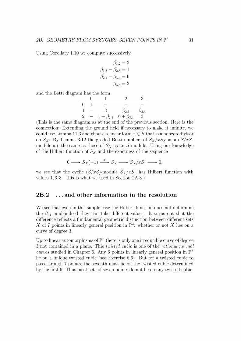
2B. GEOMETRY FROM SYZYGIES: SEVEN POINTS IN P3 31
Using Corollary 1.10 we compute successively
β1,2 = 3
β1,3 − β2,3 = 1
β2,4 − β3,4 = 6
β3,5 = 3
and the Betti diagram has the form0 1 2 3
0 1 − − −1 − 3 β2,3 β3,4
2 − 1 + β2,3 6 + β3,4 3(This is the same diagram as at the end of the previous section. Here is theconnection: Extending the ground field if necessary to make it infinite, wecould use Lemma 11.3 and choose a linear form x ∈ S that is a nonzerodivisoron SX . By Lemma 3.12 the graded Betti numbers of SX/xSX as an S/xS-module are the same as those of SX as an S-module. Using our knowledgeof the Hilbert function of SX and the exactness of the sequence
0 - SX(−1)x- SX - SX/xSx - 0,
we see that the cyclic (S/xS)-module SX/xSx has Hilbert function withvalues 1, 3, 3—this is what we used in Section 2A.3.)
2B.2 . . . and other information in the resolution
We see that even in this simple case the Hilbert function does not determinethe βi,j, and indeed they can take different values. It turns out that thedifference reflects a fundamental geometric distinction between different setsX of 7 points in linearly general position in P3: whether or not X lies on acurve of degree 3.
Up to linear automorphisms of P3 there is only one irreducible curve of degree3 not contained in a plane. This twisted cubic is one of the rational normalcurves studied in Chapter 6. Any 6 points in linearly general position in P3
lie on a unique twisted cubic (see Exercise 6.6). But for a twisted cubic topass through 7 points, the seventh must lie on the twisted cubic determinedby the first 6. Thus most sets of seven points do not lie on any twisted cubic.

32 CHAPTER 2. FIRST EXAMPLES OF FREE RESOLUTIONS
((Figure 2))
Theorem 2.4. Let X be a set of 7 points in linearly general position inP3. There are just two distinct Betti diagrams possible for the homogeneouscoordinate ring SX :
0 1 2 30 1 − − −1 − 3 − −2 − 1 6 3
and
0 1 2 30 1 − − −1 − 3 2 −2 − 3 6 3
In the first case the points do not lie on any curve of degree 3. In the secondcase, the ideal J generated by the quadrics containing X is the ideal of theunique curve of degree 3 containing X, which is irreducible.
Proof. Let q0, q1, q2 be three quadratic forms that span the degree 2 part ofI := IX . A linear syzygy of the qi is a vector (a0, a1, a2) of linear forms with∑2i=0 aiqi = 0. We will focus on the number of independent linear syzygies,
which is β2,3.
If β2,3 = 0, then by Proposition 1.9 we also have β3,4 = 0 and the computationof the differences of the βi,j above shows that the Betti diagram of SX =S/I is the first of the two given tables. As we shall see in Chapter 6, anyirreducible curve of degree ≤ 2 lies in a plane. Since the points of X arein linearly general position, they are not contained in the union of a lineand a plane, or the union of 3 lines, so any degree 3 curve containing X isirreducible. Further, if C is an irreducible degree 3 curve in P3, not containedin a plane, then the C is a twisted cubic, and the ideal of C is generated bythree quadrics, which have 2 linear syzygies. Thus in the case where X iscontained in a degree 3 curve we have β2,3 ≥ 2.
Now suppose β2,3 > 0, so that there is a nonzero linear syzygy∑2i=0 aiqi =
0. If the ai were linearly dependent then we could rewrite this relation asa′1q
′1 + a′2q
′2 = 0 for some independendent quadrics q′1 and q′2 in I. By unique
factorization, the linear form a′1 would divide q′2; say q′2 = a′1b. Thus Xwould be contained in the union of the planes a′1 = 0 and b = 0, and one ofthese planes would contain four points of X, contradicting our hypothesis.Therefore the a0, a1, a2 are linearly independent linear forms.
Changing coordinates on P3 we can harmlessly assume that ai = xi. Wecan then read the relation
∑xiqi = 0 as a syzygy on the xi. But from the
exactness of the Koszul complex (see for example Theorem 2.1 as applied inexample b of Section 2A.2), we know that all the syzygies of x0, x1, x2 are

2B. GEOMETRY FROM SYZYGIES: SEVEN POINTS IN P3 33
given by the columns of the matrix 0 x2 −x1
−x2 0 x0
x1 −x0 0
,and thus we must have q0q1
q2
=
0 x2 −x1
−x2 0 x0
x1 −x0 0
b0b1b2
for some linear forms bi. Another way to express this equation is to say thatqi is (−1)i times the determinant of the 2× 2 matrix formed by omitting thei-th column of the matrix
M =(x0 x1 x2
b0 b1 b2
),
where the columns are numbered 0, 1, 2. The two rows of M are independentbecause the qi, the minors, are nonzero. (Throughout this book we willfollow the convention that a minor of a matrix is a subdeterminant times anappropriate sign.)
We claim that both rows of M give relations on the qi. The vector (x0, x1, x2)is a syzygy by virtue of our choice of coordinates. To see that (b0, b1, b2) isalso a syzygy, note that the Laplace expansion of
det
x0 x1 x2
b0 b1 b2b0 b1 b2
is∑i biqi. However, this 3×3 matrix has a repeated row, so the determinant is
0, showing that∑i biqi = 0. Since the two rows ofM are linearly independent,
we see that the qi have (at least) 2 independent syzygies with linear formsas coefficients.
The ideal (q0, q1, q2) ⊂ I that is generated by the minors of M is unchangedif we replace M by a matrix PMQ where P and Q are invertible matrices ofscalars. It follows that matrices of the form PMQ cannot have any entriesequal to zero. This shows that M is “1-generic” in the sense of Chapter 6and it follows from Theorem 6.4 that the ideal J = (q0, q1, q2) ⊂ I is prime

34 CHAPTER 2. FIRST EXAMPLES OF FREE RESOLUTIONS
and of codimension 2—that is, J defines an irreducible curve C containingX in P3.
From Theorem 3.2 it follows that a free resolution of SC may be written as
0 → S2(−3)
x0 b0x1 b1x2 b2
- S3(−2)
(q0 q1 q2 )- S - SC → 0.
From the resolution of SC we can also compute its Hilbert function:
HSC(d) =
(3 + d
3
)− 3
(3 + d− 2
3
)+ 2
(3 + d− 3
3
)= 3d+ 1 for d ≥ 0.
Thus the Hilbert polynomial of the curve is 3d+ 1.
For large d the higher cohomology H i(OC(d)) vanishes by Serre’s Theo-rem ([Hartshorne 1977, Theorem 5.2]) so that the Euler characteristic isχ(OC(d)) :=
∑i(−1)i dimK Hi(OC(d)) = 3d+1. It follows from the Riemann-
Roch Theorem that C is a cubic curve as claimed.
It may be surprising that in Theorem 2.4 the only possibilities for β2,3 are 0and 2, and that β3,4 is always 0. These restrictions are removed, however, ifone looks at sets of 7 points that are not in linearly general position thoughthey have the same Hilbert function as a set of points in linearly generalposition; some examples are given in Exercises 2.11–2.12.
2C Exercises
1. If m1, . . . ,mn are monomials in S, show that the projective dimensionof S/(m1, · · · ,mn) is at most n. No such principle holds for arbitraryhomogeneous polynomials; see Exercise 2.4.
2. Let 0 ≤ n ≤ r. Show that if M is a graded S-module which containsa submodule isomorphic to S/(x0, . . . , xn) (so that (x0, . . . , xn) is anassociated prime of M) then the projective dimension of M is at least

2C. EXERCISES 35
n + 1. If n + 1 is equal to the number of variables in S, show thatthis condition is necessary as well as sufficient. (Hint: For the laststatement, use the Auslander-Buchsbaum theorem, Theorem 11.11.)
3. Consider the ideal I = (x0, x1) ∩ (x2, x3) of two skew lines in P3.
((Figure 4))
Prove that I = (x0x2, x0x3, x1x2, x1x3), and compute the minimal freeresolution of S/I. In particular, show that S/I has projective dimension3 even though its associated primes are precisely (x0, x1) and (x2, x3),which have height only 2. Thus the principle of Exercise 2.2 can’t beextended to give the projective dimension in general.
4. Show that the ideal J = (x0x2 − x1x3, x0x1, x2x3) defines the unionof two (reduced) lines in P3, but is not equal to the saturated idealof the two lines. Conclude that the projective dimension of S/J is 4(you might use the Auslander-Buchsbaum formula, Theorem 11.35).In fact, three-generator ideals can have any projective dimension; see[Bruns 1976] or [Evans and Griffith 1985, Corollary 3.13].
5. LetM be a finitely generated graded S-module, and letBj =∑i(−1)iβi,j(M).
Show from Proposition 2.3 that
Bj =∑i
(−1)iHM(j)
(r + 1
j
).
This is another form of the formula in Corollary 1.10.
6. Show that if M is a graded S module, then
β0,j(M) = HM(j)
if and only if mM = 0.
7. If M is a graded S-module, show that
βi,j(M) ≥HM(j − i)
(r + 1
i
)
−HM(j − i+ 1)
(r + 1
i− 1
)
−HM(j − i− 1)
(r + 1
i+ 1
).

36 CHAPTER 2. FIRST EXAMPLES OF FREE RESOLUTIONS
8. Prove that the complex
0 → S2(−3)
x0 x1
x1 x2
x2 x3
- S3(−2)
(x1x3−x22 −x0x3+x1x2 x0x2−x2
1)- S
is indeed a resolution of the homogeneous coordinate ring SC of thetwisted cubic curve C by the following steps:
(a) Identify SC with the subring of K[s, t] consisting of those gradedcomponents whose degree is divisible by 3. Show in this way thatHSC
(d) = 3d+ 1 for d ≥ 0.
(b) Compute the Hilbert functions of the terms S, S3(−2), and S2(−3).Show that their alternating sum HS −HS3(−2) +HS2(−3) is equalto the Hilbert function HSC
.
(c) Show that the map
S2(−3)
x0 x1
x1 x2
x2 x3
- S3(−2)
is a monomorphism. As a first step you might prove that it be-comes a monomorphism when the polynomial ring S is replacedby its quotient field, the field of rational functions.
(d) Show that the results in 2.8 and 2.8 together imply that the com-plex exhibited above is a free resolution of SC .
9. Let X be a set of n ≤ 2r + 1 points in Pr in linearly general position.Show that X imposes independent conditions on quadrics: that is,show that the space of quadratic forms vanishing on X is
(r+22
)− n
dimensional. (It is enough to show that for each p ∈ X there is aquadric not vanishing on p but vanishing at all the other points of X.)Use this to show that X imposes independent conditions on forms ofdegree ≥ 2. The same idea can be used to show that and n ≤ dr + 1points in linearly general position impose independent conditions onforms of degree d.
Deduce the correctness of the Hilbert function for 7 points in linearlygeneral position given by the table in Section 2B.1.

2C. EXERCISES 37
10. The sufficient condition of Exercise 2.9 is far from necessary. Oneway to sharpen it is to use Edmonds’ Theorem, which is the followingbeautiful and nontrivial theorem in linear algebra ([Edmonds 1965]).((Find an accessible reference for this story!))
Theorem 2.5. If v1, . . . , vds are vectors in an s-dimensional vectorspace then the list (v1, . . . , vds) can be written as the union of d bases ifand only if no dk + 1 of the vectors vi lie in a k-dimensional subspace,for every k.
Now suppose that Γ is a set of at most 2r+ 1 points in Pr, and, for allk < r, each set of 2k+1 points of Γ spans at least a (k+1)-plane. UseEdmonds’ Theorem to show that Γ imposes independent conditions onquadrics in Pr (Hint: You can apply Edmonds’ Theorem to the setobtained by counting one of the points of Γ twice.)
11. Show that if X is a set of 7 points in P3 with 6 points on a plane, butnot on any conic curve in that plane, while the seventh point does notline in the plane, then X imposes independent conditions on forms ofdegree ≥ 2 and β2,3 = 3.
12. Let Λ ⊂ P3 be a plane, and let D ⊂ Λ be an irreducible conic. Choosepoints p1, p2 /∈ Λ such that the line joining p1 and p2 does not meetD. Show that if X is a set of 7 points in P3 consisting of p1, p2 and5 points on D, then X imposes independent conditions on forms ofdegree ≥ 2 and β2,3 = 1. (Hint: To show that β2,3 ≥ 1, find a pairof reducible quadrics in the ideal having a common component. Toshow that β2,3 ≤ 1, show that the quadrics through the points are thesame as the quadrics containing D and the two points. There is, upto automorphisms of P3, only one configuration consisting of a conicand two points in P3 such that the line though the two points does notmeet the conic. You might produce such a configuration explicitly andcompute the quadrics and their sysygies.)
13. Show that the labeled simplicial complex
((Figure 5))
gives a nonminimal free resolution of the monomial ideal (x0x1, x0x2, x1x2, x2x3).Use this to prove that the Betti diagram of a minimal free resolution is
0 1 2 30 1 − − −1 − 4 4 1

38 CHAPTER 2. FIRST EXAMPLES OF FREE RESOLUTIONS
14. Use the Betti diagram in Exercise 2.13 to show that the minimal freeresolution of (x0x1, x0x2, x1x2, x2x3) cannot be written as C(∆) for anylabeled simplicial complex ∆. (It can be written as the free complexcoming from a certain topological cell complex; for this generalizationsee [Bayer and Sturmfels 1998].)
15. Show the ideal
I = (x3, x2y, x2z, y3) ⊂ S = K[x, y, z]
has minimal free resolution C(∆), where ∆ is the labeled simplicialcomplex
((Figure 18.))
Compute the Betti diagram, the Hilbert function, and the Hilbert poly-nomial of S/I, and show that in this case the bound given in Corollary1.3 ((I think this is now a forward reference to something thatdoes not exist.)) is not sharp. Can you see easily from the Bettidiagram why this happens?

Chapter 3
Points in P2
Revised 8/12/03
The first case in which the relation of syzygies and geometry becomes clear,and the one in which it is best understood, is the case where the geometricobjects are finite sets of points in P2. We will devote this chapter to such sets.(The reader who knows about schemes, for example at the level of the firsttwo chapters of Eisenbud-Harris [Eisenbud and Harris 2000], will see thatexactly the same considerations apply to finite schemes in P2.) Of coursethe only intrinsic geometry of a set of points is the number of points, andwe will see that this is the data present in the Hilbert polynomial. But a setof points embedded in projective space has plenty of extrinsic geometry. Forexample, it is interesting to ask what sorts of curves a given set of points lieson, or to ask about the geometry of the dual hyperplane arrangement (see[Orlik and Terao 1992]), or about the embedding of the “Gale transform” ofthe points (see [Eisenbud and Popescu 1999]). All of these things have someconnections with syzygies.
Besides being a good model problem, the case of points in P2 arises directlyin considering the plane sections of varieties of codimension 2, such as thevery classical examples of curves in P3 and surfaces in P4. For example,a knowledge of the possible Hilbert functions of sets of points in “uniformposition” is the key ingredient in “Castelnuovo Theory”, which treats thepossible genera of curves in P3 and related problems.
39

40 CHAPTER 3. POINTS IN P2
Despite this wealth of related topics, the goal of this chapter is modest:We will characterize the Betti diagrams of the possible minimal graded freeresolutions of ideals of forms vanishing on sets of points in P2, and begin torelate these discrete invariants to geometry in simple cases.
Throughout this chapter, S will denote the graded ring K[x0, x1, x2]. All theS-modules we consider will be finitely generated and graded. Such a moduleadmits a minimal free resolution, unique up to isomorphism. By Corollary1.8, its length is equal to the module’s projective dimension.
3A The ideal of a finite set of points
The simplest ideals are principal ideals. As a module, such an ideal is free.The next simplest case is perhaps that of an ideal having a free resolution oflength 1, and we will see that the ideal of forms vanishing on any finite setof points in P2 has this property.
We will write pd I for the projective dimension of I. By the depth of agraded ring, we mean the grade of the irrelevant ideal—that is, the lengthof a maximal regular sequence of homogeneous elements of positive degree.(The homogeneous case is very similar to the local case; for example, allmaximal regular sequences have the same length in the homogeneous caseas in the local case, and the local proofs can be modified to work in thehomogeneous case. For a systematic treatement see [Goto and Watanabe1978a] and [Goto and Watanabe 1978b].)
Proposition 3.1. If I ⊂ S is the homogeneous ideal of a finite set of pointsin P2, then I has a free resolution of length 1.
Proof. Suppose I = I(X), the ideal of forms vanishing on the finite setX ⊂ P2. By the Auslander-Buchsbaum Formula (Theorem 11.11 we have
pd S/I = depth(S)− depth(S/I).
But depth(S/I) ≤ dim(S/I) = 1. The ideal I is the intersection of theprime ideals of forms vanishing at the individual points of X, so the max-imal homogeneous ideal m of S is not associated to I. This implies thatdepth(S/I) > 0. Also, the depth of S is 3 (the variables form a maximal

3A. THE IDEAL OF A FINITE SET OF POINTS 41
homogeneous regular sequence). Thus pd S/I = 3−1 = 2, whence pd I = 1,as I is the first module of syzygies in a free resolution of S/I.
It turns out that ideals with a free resolution of length 1 are determinantal(see Appendix 11G for some results about determinantal ideals.) This resultwas discovered by Hilbert in a special case and by Burch in general.
3A.1 The Hilbert-Burch Theorem
In what follows, we shall work over an arbitrary Noetherian ring R. (Evenmore general results are possible; see for example [Northcott 1976].) For anymatrix M with entries in R we write It(M) for the ideal generated by thet× t subdeterminants of M The length of a maximal regular sequence in anideal I is written grade(I).
Theorem 3.2 (Hilbert-Burch). Suppose that an ideal I in a Noetherianring R admits a free resolution of length 1
0 - FM- G - I - 0.
If the rank of the free module F is t, then the rank of G is t + 1, and thereexists a nonzerodivisor a such that I = aIt(M). Regarding M as a matrixwith respect to given bases of F and G, the generator of I that is the imageof the i-th basis vector of G is ±a times the determinant of the submatrix ofM formed from all except the i-th row. Moreover, the grade of It(M) is 2.
Conversely, given a (t+1)×t matrix M with entries in R such that grade It(M) ≥2 and a nonzerodivisor a of R, the ideal I = aIt(M) admits a free resolutionof length 1 as above. The ideal I has grade 2 if and only if the element a isa unit.
In view of the signs that appear in front of the determinants, we define thet × t minor of M to be (−1)i detM ′
i , where M ′i is the matrix M ′ with the
i-th row omitted. We can then say that the generator of I that is the imageof the i-th basis vector of G is a times the i-th minor of M .
We postpone the proof in order to state a general result describing free reso-lutions. If ϕ is a map of free R-modules, we write rank(ϕ) for the rank (that

42 CHAPTER 3. POINTS IN P2
is, the largest size of a nonvanishing minor) and I(ϕ) for the determinantalideal Irank(ϕ)(ϕ). For any map ϕ of free modules we make the conventionthat I0(ϕ) = R. In particular, if ϕ is the zero map, then the rank of ϕ is 0 soI(ϕ) := I0(ϕ) = R. We also take depth(R,R) = ∞, so that grade(I(ϕ)) = ∞in this case.
Theorem 3.3 (Buchsbaum-Eisenbud). A complex of free modules
F : 0 - Fmϕm- Fm−1
- · · · - F1ϕ1- F0
over a Noetherian ring R is exact if and only if, for every i,
1. rankϕi+1 + rankϕi = rankFi.
2. depth(I(ϕi)) ≥ i.
For a proof of Theorem 3.3 see Eisenbud [Eisenbud 1995, Theorem 20.9]. Itis crucial that the complex be finite and begin with a zero on the left; nosimilar result is known without such hypotheses.
In the special case where R is a polynomial ring R = K[x0, . . . , xr] and Kis algebraically closed, Theorem 3.3 has a simple geometric interpretation.We think of R as a ring of functions on Kr+1 (in the graded case we couldwork with Pr instead.) If p ∈ Kr+1, we write I(p) for the ideal of functionsvanishing at p, and we write
F(p) : 0 - Fm(p)ϕm(p)- · · · ϕ1(p)- F0(p)
for the result of tensoring F with the residue field κ(p) := R/I(p), regardedas a complex of finite dimensional vector spaces over κ(p). A matrix for themap ϕi(p) is obtained simply by evaluating a matrix for the map ϕi at p.Theorem 3.3 expresses the relation between the exactness of the complex offree modules F and the exactness of the complexes of vector spaces F(p).
Corollary 3.4. Let
F : 0 - Fmϕm- Fm−1
- · · · - F1ϕ1- F0
be a complex of free modules over the polynomial ring S = K[x0, . . . , xr],where K is an algebraically closed field. Let Xi ⊂ Kr+1 be the set of pointsp such that the evaluated complex F(p) is not exact at Fi(p). The complex Fis exact if and only if, for every i, the set Xi is empty or codimXi ≥ i.

3A. THE IDEAL OF A FINITE SET OF POINTS 43
Proof. Set ri = rankFi − rankFi+1 + . . . ± rankFm. Theorem 3.3 impliesthat F is exact if and only if grade Iri(ϕi) ≥ i for each i ≥ 1. First, if F isexact then by descending induction we see from condition 1 of the Theoremthat rankϕi = ri for every i, and then the condition grade Iri(ϕi) ≥ i is justcondition 2 of Theorem 3.3.
Conversely, suppose that grade Iri(ϕi) ≥ i. It follows that rankϕi ≥ rifor each i. Tensoring with the quotient field of R we see that rankϕi+1 +rankϕi ≤ rankFi in any case. Using this and the previous inequality, we seeby descending induction that in fact rankϕi = ri for every i, so conditions 1and 2 of Theorem 3.3 are satisfied.
Now let
Yi = p ∈ Kr+1 | rankϕi(p) < ri.
Thus Yi is the algebraic set defined by the ideal Iri(ϕi). Since the polynomialring S is Cohen-Macaulay (Theorem 11.20) the grade of Iri(ϕi) is equal tothe codimension of this ideal, which is the same as the codimension of Yi. Itfollows that F is exact if and only if the codimension of Yi in Kr+1 is ≥ i foreach i ≥ 1.
On the other hand, the complex of finite-dimensional K-vector spaces F(p)is exact at Fj(p) if and only if rankϕj+1(p) + rankϕj(p) = rankFj(p). SinceF(p) is a complex, this is the same as saying that rankϕj+1(p)+rankϕj(p) ≥rankFj(p). This is true for all j ≥ i if and only if rankϕj(p) ≥ rj for allj ≥ i. Thus F(p) is exact at Fj(p) for all j ≥ i if and only if p /∈ ⋃j≥i Yj.The codimension of
⋃j≥i Yj is the minimum of the codimensions of the Yj for
j ≥ i. Thus codim⋃j≥i Yj ≥ i for all i if and only if codimYi ≥ i for all i.
Thus F satisfies the condition of the Corollary if and only if F is exact.
Example 3.1. To illustrate these results, we return to the example of Ex-ercise 2.8 from Chapter 2, and consider the complex
F : 0 → S2(−3)
ϕ2=
x0 x1
x1 x2
x2 x3
- S3(−2)
ϕ1=(x1x3−x22 −x0x3+x1x2 x0x2−x2
1)- S.
In the notation of the proof of 3.4 we have r2 = 2, r1 = 1. Further, theentries of ϕ1 are the 2 × 2 minors of ϕ2, as in Theorem 3.2 with a = 1. In

44 CHAPTER 3. POINTS IN P2
particular Y1 = Y2 and X1 = X2. Thus Corollary 3.4 asserts that F is exact ifand only if codimX2 ≥ 2. But X2 consists of the points p where ϕ2 fails to bea monomorphism—that is, where rank(ϕ(p)) ≤ 1. If p = (p0, . . . , p3) ∈ X2
and p0 = 0 then, inspecting the matrix ϕ2 we see that p1 = p2 = 0, sop = (0, 0, 0, p3). Such points form a set of codimension 3 in K4. On the otherhand, if p ∈ X2 and p0 6= 0 then set again inspecting the matrix ϕ2 we seethat p2 = (p1/p0)
2, p3 = (p1/p0)3. Thus p is determined by the 2 parameters
p0, p1, and the set of such p has codimension ≥ 4− 2 = 2. In particular X2,the union of these two sets, has codimension ≥ 2, so F is exact by Corollary3.4.
In this example all the ideals are homogeneous, and the projective algebraicset X2 is in fact the twisted cubic curve.
A consequence of Theorem 3.2 in the general case is that any ideal with afree resolution of length 1 contains a nonzerodivisor. Theorem 3.3 allows usto prove a more general result of Auslander and Buchsbaum:
Corollary 3.5 (Auslander-Buchsbaum). If an ideal I has a finite freeresolution, then I contains a nonzerodivisor.
In the non-graded, non-local case, having a finite projective resolution (finiteprojective dimension) would not be enough; for example, if k is a field thenthe ideal k×0 ⊂ k×k is projective, but does not contain a nonzerodivisor.
Proof. In the free resolution
0 - Fnϕn- · · · ϕ2- F1
ϕ1- R - R/I - 0
the ideal I(ϕ1) is exactly I. By Theorem 3.3 it has grade at least 1.
The proof of the last statement of Theorem 3.2 depends on the followingidentity:
Lemma 3.6. If M is a (t + 1) × t matrix over a commutative ring R, anda ∈ R, then the composition
Rt M- Rt+1 ∆- R

3A. THE IDEAL OF A FINITE SET OF POINTS 45
is zero, where the map ∆ is given by the matrix ∆ = (a∆1, · · · , a∆t+1), theelement ∆i being the t× t minor of M omitting the i-th row (remember thatby definition this minor is (−1)i times the determinant of the correspondingsubmatrix.)
Proof. Write ai,j for the (i, j) entry of M . The i-th entry of the compositemap ∆M is a
∑j ∆jai,j, that is, a times the Laplace expansion of the deter-
minant of the (t+1)× (t+1) matrix obtained from M by repeating the i-thcolumn. Since any matrix with a repeated row has determinant zero, we get∆M = 0.
Proof of Theorem 3.2. We prove the last statement first: suppose that thegrade of It(M) is at least 2 and a is a nonzerodivisor. It follows that therank of M is t, so that I(M) = It(M), and the rank of ∆ is 1. ThusI(∆) = I1(∆) = aI(M) and the grade of I(∆) is at least 1. By Theorem 3.3
0 - FM- G - I - 0.
is the resolution of I = aI(M) as required.
We now turn to the first part of Theorem 3.2. Using the inclusion of theideal I in R, we see that there is a free resolution of R/I of the form
0 - FM- G
A- R.
Since A is nonzero it has rank 1, and it follows from Theorem 3.3 that therank of M must be t, and the rank of G must be t + 1. Further, the gradeof I(M) = It(M) is at least 2. Theorem 11.32 shows that the codimensionof the ideal of t× t minors of a (t+ 1)× t matrix is at most 2. By Theorem11.7 the codimension is an upper bound for the grade, so grade I(M) = 2.Write ∆ = (∆1, . . . ,∆t+1), for the 1× (t+1) matrix whose entries ∆i are theminors of M as in Lemma 3.6. Writing −∗ for HomR(−, R), it follows fromTheorem 3.3 that the sequence
F ∗ M∗G∗ ∆∗
R 0,
which is a complex by Lemma 3.6, is exact. On the other hand, the image ofthe map A∗ is contained in the kernel of M∗, so that there is a map a : R→ R

46 CHAPTER 3. POINTS IN P2
such that the diagram
F ∗ M∗
G∗ A∗
R
F ∗
wwwwwwwwwwwww
M∗G∗
wwwwwwwwwwwww
∆∗R
a
?
.................
commutes. The map a is represented by a 1× 1 matrix whose entry we alsocall a. By Corollary 3.5, the ideal I contains a nonzerodivisor. But from thediagram above we see that I = aIt(M) is contained in (a), so a must be anonzerodivisor.
As It(M) has grade 2, the ideal I = aIt(M) has grade 2 if and only if a is aunit. With Theorem 3.3 this completes the proof.
3A.2 Invariants of the resolution
The Hilbert-Burch Theorem just described allows us to exhibit some interest-ing numerical invariants of a set X of points in P2. Throughout this sectionwe will write I = IX ⊂ S for the homogeneous ideal of X, and SX = S/IX forthe homogeneous coordinate ring of X. By Proposition 3.1 the ideal IX hasprojective dimension 1, and thus SX has projective dimension 2. Supposethat the minimal graded free resolution of SX has the form
F : 0 → FM- G - S,
where G is a free module of rank t+ 1. By Theorem 3.2, the rank of F is t.
We can exhibit the numerical invariants of this situation either by using thedegrees of the generators of the free modules or the degrees of the entriesof the matrix M . We write the graded free modules G and F in the formG =
⊕t+11 S(−ai) and F =
⊕t1 S(−bi), where, as always, S(−a) denotes the
free module of rank 1 with generator in degree a. The ai are thus the degreesof the minimal generators of I. The degree of the (i, j) entry of the matrixM is then bj − ai. As we shall soon see, the degrees of the entries on thetwo principal diagonals of M determine all the other invariants. We writeei = bi − ai and fi = bi − ai+1 for these degrees.

3A. THE IDEAL OF A FINITE SET OF POINTS 47
To make the data unique, we assume that the bases are ordered so that a1 ≥· · · ≥ at+1 and b1 ≥ · · · ≥ bt or, equivalently, so that fi ≥ ei and fi ≥ ei+1.Since the generators of G correspond to rows of M and the generators of Fcorrespond to columns of M , and the ei and fi are degrees of entries of M ,we can exhibit the data schematically as follows:
b1 b2 · · · bta1 e1 ∗ · · · ∗a2 f1 e2 · · · ∗...
.... . . . . .
...at ∗ · · · ft−1 etat+1 ∗ · · · ∗ ft
The case of 8 general points in P2 is illustrated on the cover of this book.((Refers to Figure 6 — should it be at the top of this Ch in-stead?)) Since minimal free resolutions are unique up to isomorphism, theintegers ai, bi, ei, fi are invariants of the set of points X. They are not ar-bitary, however, but are determined (for example) by the ei and fi. The nextproposition gives these relations. We shall see at the very end of this chapterthat Proposition 3.7 gives all the restrictions on these invariants, so that itdescribes the numerical characteristics of all possible free resolutions of setsof points.
Proposition 3.7. If
F : 0 →t∑1
S(−bi)M-
t+1∑1
S(−ai) - S,
is a minimal graded free resolution of S/I, and ei, fi denote the degrees ofthe entries on the principal diagonals of M , then for all i,
• ei ≥ 1, fi ≥ 1.
• ai =∑j<i
ej +∑j≥i
fj.
• bi = ai + ei for i = 1, . . . , t and∑t
1 bi =∑t+1
1 ai.
If the bases are ordered so that a1 ≥ · · · ≥ at+1 and b1 ≥ · · · ≥ bt then inaddition

48 CHAPTER 3. POINTS IN P2
• fi ≥ ei, fi ≥ ei+1.
Proposition 3.7 gives an upper bound on the minimal number of generatorsof the ideal of a set of points that are known to lie on a curve of given degree.Burch’s motivation in proving her version of the Hilbert-Burch theorem wasto generalize this bound, which was known independently.
Corollary 3.8. If I is the homogeneous ideal of a set of points in P2 lyingon a curve of degree d, then I can be generated by d+ 1 elements.
Proof of Corollary 3.8. If t+1 is the minimal number of generators of I then,by Proposition 3.7, the degree ai of the i-th minimal generator is the sumof t numbers that are each at least 1, so t ≤ ai. Since I contains a form ofdegree d we must have ai ≤ d for some i.
Hilbert’s method for computing the Hilbert function, described in Chapter1, allows us to compute the Hilbert function and polynomial of SX in termsof the ei and fi. As we will see in Section 4A.1, HX(d) is constant for larged, and its value is the number of points in X, usually called the degree ofX and written degX. If X were the complete intersection of a curve ofdegree e with a curve of degree f , then in the notation of Proposition 3.7we would have t = 1, e1 = e f1 = f , and by Bezout’s Theorem the degreeof X would be ef = e1f1. The following is the generalization to arbitraryt, discovered by Ciliberto, Geramita, and Orrechia [Ciliberto et al. 1986].For the generalization to determinantal varieties of higher codimension seeHerzog and Trung [Herzog and Trung 1992, Corollary 6.5].
Corollary 3.9. If X is a finite set of points in P2 then, with notation asabove,
degX =∑i≤j
eifj.
The proof is straightforward calculation from Proposition 3.7, and we leaveit and a related formula to the reader in Exercise 3.14.
Proof of Proposition 3.7. Since I has codimension 2 and S is a polynomialring (and thus Cohen-Macaulay) I has grade 2. It follows that the non-zerodivisor a that is associated to the resolution F as in Theorem 3.2 is a

3B. EXAMPLES 49
unit. Again because S is a polynomial ring this unit must be a scalar. Thusthe ai are the degrees of the minors of M .
We may assume that the bases are ordered as in the last statement of theProposition. We first show that the ei (and thus also, by our ordering con-ventions, the fi) are at least 1. Write mi,j for the (i, j) entry of M . By theminimality of F, no mi,j can be a nonzero constant, so that if ei ≤ 0 thenmi,i = 0. Moreover if p ≤ i and q ≥ i then
degmp,q = bq − ap ≤ bi − ai = ei,
by our ordering of the bases. If ei ≤ 0 then mp,q = 0 for all (p, q) in thisrange, as in the following diagram, where t = 4 and we assume e3 ≤ 0:
M =
∗ ∗ 0 0∗ ∗ 0 0∗ ∗ 0 0∗ ∗ ∗ ∗∗ ∗ ∗ ∗
.
We see by calculation that the determinant of the upper t × t submatrix ofM vanishes. By Theorem 3.2 this determinant is a minimal generator of I,and this is a contradiction.
The identity ai =∑j<i
ej +∑j≥i
fj again follows from Theorem 3.2, since ai is
the degree of the determinant ∆i of the submatrix of M omitting the i-throw, and one term in the expansion of this determinant is
∏j<i
mj,j ·∏j≥i
mj+1,j.
Since ei = bi − ai. we get∑t
1 bi =∑t
1 ai +∑t
1 ei =∑t+1
1 ai.
3B Examples
3B.1 Points on a conic
We illustrate the theory above, in particular Corollary 3.8, by discussing thepossible resolutions of a set of points lying on an irreducible conic.
((Figure 7a))

50 CHAPTER 3. POINTS IN P2
For the easy case of points on a line, and the more complicated case of pointson a reducible conic, see Exercises 3.1 and 3.4–3.7 below.
Suppose now that the point set X ⊂ P2 does not lie on any line, but doeslie on some conic, defined by a quadratic form q. In the notation of Proposi-tion 3.7 we have at+1 = 2. Since at+1 =
∑t1 ei it follows from Proposition 3.7
that either t = 1, e1 = 2 or else t = 2 and e1 = e2 = 1.
1. If t = 1 then X is a complete intersection of the conic with a curveof degree a1 = d defined by a form g. By our formula (or Bezout’sTheorem), the degree of X is 2d. Note in particular that it is even. Wehave b1 = d + 2, and the resolution takes the following form (see alsoTheorem 11.28):
S(−2)
g * HHHHqj
0 - S(−d− 2) ⊕ S −→ SXHHHH−q j
g
*
S(−d)
((Silvio: this diagram has the same problems as the similarone in this chapter.)) In the case d = 2 the Betti diagram of thisresolution is
0 1 20 1 − −1 − 2 −2 − − 1
while for larger d it takes the form0 1 2
0 1 − −1 − 1 −2 − − −...
.
.....
.
..d− 2 − − −d− 1 − 1 −
d − − 1
2. The other possibility is that t = 2 and e1 = e2 = 1. We will treat onlythe case where the conic q = 0 is irreducible, and leave the reduciblecase to the reader in Exercises 3.4–3.7 at the end of the chapter. ByProposition 3.7 the resolution has the form
0 - S(−1− f1 − f2)⊕ S(−2− f2)M- S(−f1 − f2)⊕ S(−1− f2)⊕ S(−2) - S

3B. EXAMPLES 51
where we assume that f1 ≥ e1 = 1, f1 ≥ e2 = 1, and f2 ≥ e2 = 1 asusual. If there are two quadratic generators, we further assume thatthe last generator is q.
By Theorem 3.2, q is (a multiple of) the determinant of the 2×2 matrixM ′ formed from the first two rows of M . Because q is irreducible, allfour entries of the upper 2× 2 submatrix of M must be nonzero. Theupper right entry of M has degree e1 + e2 − f1 ≤ 1. If it were ofdegree 0 then by the supposed minimality of the resolution it wouldbe 0, contradicting the irreducibility of q. Thus e1 + e2 − f1 = 1, sof1 = 1. By our hypothesis a3 = 2, and it follows from Proposition 3.7that a1 = a2 = 1 + f2, b1 = b2 = 2 + f2. We deduce that the resolutionhas the form
0 - S(−2− f2)2 M- S(−1− f2)
2 ⊕ S(−2) - S.
If f2 = 1 then the Betti diagram is0 1 2
0 1 0 01 0 3 2
while if f2 > 1 it has the form0 1 2
0 1 − −1 − 1 −2 − − −...
..
....
..
.f2 − 1 − − −
f2 − 2 2
Applying the formula of Corollary 3.9 we get degX = 2f2 + 1. Inparticular, we can distinguish this case from the complete intersectioncase by the fact that the number of points is odd.
3B.2 Four non-colinear points
Any 5 points lie on a conic, since the quadratic forms in 3 variables form a5-dimensional vector space, and vanishing at a point is one linear condition,so there is a nonzero quadratic form vanishing at any 5 points. Thus we canuse the ideas of the previous subsection to describe the possible resolutionsfor up to 5 points. One set of three non-colinear points in P2 is like another,so we treat the case of a set X = p1, . . . , p4 of four non-colinear points, thefirst case where geometry enters. (For the case of 3 points see Exercise 3.2.)

52 CHAPTER 3. POINTS IN P2
Since there is a 6 dimensional vector space of quadratic forms on P2, and thecondition of vanishing at a point is a single linear condition, there must beat least two distinct conics containing X.
First suppose that no three of the points lie on a line. It follows that X iscontained in the following two conics, each a union of two lines:
C1 = p1, p2 ∪ p3, p4 C2 = p1, p3 ∪ p2, p4.
In this case, X is the complete intersection of C1 and C2, and we have Bettidiagram
0 1 20 1 0 01 0 2 02 0 0 1
. ((Figure 9))
%
%%
%%
%%
cc
cc
cc
ccLLLLLLLLLL
dbdb
The two conics are the two pairs of lines containing the 4 points
On the other hand, suppose that three of the points, say p1, p2, p3 lie on aline L. Let L1 and L2 be lines through p4 that do not contain any of thepoints p1, p2, p3. It follows that X lies on the two conics
C1 = L ∪ L1 C2 = L ∪ L2,
and the intersection of these two conics contains the whole line L. ThusX is not the complete intersection of these two conics containing it, so byCorollary 3.8 the ideal of X requires exactly 3 generators. From Propositions3.7 and 3.9 it follows that
e1 = e2 = 1, f1 = 2, f2 = 1,
and the ideal I of X is generated by the quadrics defining C1 and C2 togetherwith a cubic equation. ((Figure 10))

3C. EXISTENCE OF SETS WITH GIVEN INVARIANTS 53
(((((((((((((((((((((
##
##
##
##
##
##
###
aaaaaaaaaaaaaaaaaa
ee
e e
Four points, three on a line, are the intersection of two conics and a cubic
The Betti diagram will be0 1 2
0 1 0 01 0 2 12 0 1 1
3C The existence of sets of points with given
numerical invariants
This section is devoted to a proof of the following converse of Proposition3.7:
Theorem 3.10. If the ground field K is infinite and ei, fi ≥ 1, for i =1, . . . , t, are integers, then there is a set of points X ⊂ P2 such that SX hasa minimal free resolution whose second map has diagonal degrees ei and fias in Proposition 3.7.
The proof is in two parts. In the next section we show that there is amonomial ideal J ⊂ K[x, y] (that is, an ideal generated by monomials in thevariables), containing a power of x and a power of y, whose free resolution hasthe corresponding invariants. This step is rather easy. Then, given any suchmonomial ideal J we will show how to produce a set of distinct points in P2
whose defining ideal I has free resolution with the same numerical invariantsas that of J .

54 CHAPTER 3. POINTS IN P2
The second step, including Theorem 3.13, is part of a much more generaltheory, sometimes called the “polarization” of monomial ideals. We sketchits elements in the exercises at the end of this chapter.
3C.1 The existence of monomial ideals with given nu-merical invariants
Proposition 3.11. Let S = K[x, y, z], and let e1, . . . , et and f1, . . . , ft bepositive integers. For i = 1, . . . , t+ 1 set
mi =∏j<i
xej∏j≥i
yfj .
and let I = (m1, . . . ,mt+1) ⊂ S be the monomial ideal they generate. Defineai and bi by the formulas of Proposition 3.7. The ring S/I has minimal freeresolution
0 →t∑i=1
S(−bi)M-
t+1∑i=1
S(−ai) - S - S/I → 0
where
M =
xe1 0 0 · · · 0 0 0yf1 xe2 0 · · · 0 0 00 yf2 xe3 · · · 0 0 0· · · · · · · · · · · · · · · · · · · · ·0 0 0 · · · 0 yft−1 xet
0 0 0 · · · 0 0 yft
and the generator of S(−ai) maps to ±mi ∈ S.
Proof. It is easy to see that mi is the determinant of the submatrix of Momitting the i-th row. Thus by Theorem 3.2 it suffices to show that the idealof maximal minors of M has grade at least 2. But this ideal contains
∏ti=1 x
ei
and∏ti=1 y
fi .
3C.2 Points from a monomial ideal
We will prove some general results allowing us to manufacture a reducedalgebraic set having ideal with the same Betti diagram as any given monomial
3C. EXISTENCE OF SETS WITH GIVEN INVARIANTS 55
ideal, as long as the ground field K is infinite. This treatment is taken fromGeramita, Gregory and Roberts [1986].
Here is the tool we will use to show that the two resolutions have the sameBetti diagram:
Lemma 3.12. Let R be a ring. If M is an R-module and y ∈ R is anonzerodivisor both on R and on M , then any free resolution of M over Rreduces modulo (y) to a free resolution of M/yM over R/(y). Thus if R is agraded polynomial ring, M is a graded module, and y is a linear form, thenthe Betti diagram of M (over R) is the same as the Betti diagram of M/yM(over the graded polynomial ring R/(y).)
Proof. Let F : · · · → F1 → F0 be a free resolution of M . We must show thatF/yF = R/(y) ⊗R F, which is obviously a free complex of R/(y)-modules,is actually a free resolution—that is, its homology is trivial except at F0,where it is M/yM . The homology of F/yF = R/(y) ⊗R F is by definitionTorR∗ (R/(y),M). Because y is a nonzerodivisor on R, the complex 0 →R
y- R → R/(y) → 0 is exact, and it is thus a free resolution of R/(y).We can use this free resolution instead of the other to compute Tor (see forexample [Eisenbud 1995, p. 674]), and we see that TorR∗ (R/(y),M) is the
homology of the sequence 0 → My- M . Since y is a nonzerodivisor on
M , the homology is just M/yM in degree 0, as required.
We now return to the construction of sets of points. If K is infinite we canchoose r embeddings (of sets) ηi : N → K. (If K has characteristic 0, wecould choose all ηi equal to the natural embedding ηi(n) = n ∈ Z ⊂ K, butany assignment of distinct ηi(n) ∈ K will do. In general we could choose allηi to be equal, but the extra flexibility will be useful in the proof.) We use theηi to embed the set of monomials of K[x1, . . . , xr] into Pr: if m = xp11 · · ·xpr
r
we set η(m) = (1, η1(p1), . . . , ηr(pr)), and we set
fm =r∏i=1
pi−1∏j=0
(xi − ηi(j)x0).
We think of fm as the result of replacing the powers of each xi in m byproducts of the distinct linear forms xi − ηi(j)x0. Note in particular thatfm ∼= m mod (x0).

56 CHAPTER 3. POINTS IN P2
Theorem 3.13. Let K be an infinite field, with an embedding N ⊂ K asabove, and let J be a monomial ideal in K[x1, . . . , xr]. Let XJ ⊂ Pr be theset
XJ = p ∈ Nr ⊂ Pr | xp /∈ J.
The ideal IXJ⊂ S = K[x0, . . . , xr] has the same Betti diagram as J ; in fact
x0 is a nonzerodivisor modulo IXJ, and J ∼= IXJ
mod (x0). Moreover, IXJis
generated by the forms fm where m runs over a set of monomial generatorsfor J .
Examples: Before giving the proof, two examples will clarify the result:
1. In the case of a monomial ideal J in K[x1, . . . , xr] that contains a power ofeach variable xi, such as the ones in K[x, y, z] described in section 3C.1, theset XJ is finite. Thus Theorem 3.13 and Proposition 3.11 together yield theexistence of sets of points in P2 whose free resolution has arbitrary invariantssatisfying Proposition 3.7. For example, the Betti diagram
0 1 20 1 − −1 − - -2 − 1 -3 − 2 14 − - 1
corresponds to invariants (e1, e2) = (2, 1), (f1, f2) = (2, 2), and monomialideal J = (y3, x4, x3y), where we have replaced x1 by x and x2 by y tosimplify notation. We will also replace x0 by z. Assuming, for simplicity,that K has characteristic 0 and that ηi(n) = n for all i, the set of points XJ
in the affine plane z = 1 looks like ((figure 19))* * ** * ** * * *
Its ideal is generated by the polynomials
y(y − 1)(y − 2)
x(x− 1)(x− 2)y
x(x− 1)(x− 2)(x− 3).
As a set of points in projective space, it has ideal IXJ⊂ K[z, x, y] generated

3C. EXISTENCE OF SETS WITH GIVEN INVARIANTS 57
by the homogenizations
fy3 = y(y − z)(y − 2z)
fx3y = x(x− z)(x− 2z)y
fx4 = x(x− z)(x− 2z)(x− 3z).
2. Now suppose that J does not contain any power of x1. There are infinitelymany isolated points in XJ , corresponding to the elements 1, x1, x
21, . . . /∈
J . Thus XJ is not itself an algebraic set. Its Zariski closure (the smallestalgebraic set containing it) is a union of planes, as we shall see. For example,if J = (x3, x2y, xy2) then XJ and its Zariski closure are shown in Figure 20.
((Figure 20))
For the proof of Theorem 3.13 we will use the following basic properties ofthe forms fm.
Lemma 3.14. Let K be an infinite field. With notation as above:
1. If f ∈ S is a form of degree ≤ d that vanishes on η(m) ∈ Pr for everymonomial m with degm ≤ d, then f = 0.
2. fm(η(m)) 6= 0.
3. fm(η(n)) = 0 if m 6= n and deg n ≤ degm
Proof. 1. We induct on the degree d ≥ 0 and the dimension r ≥ 1. The casesin which d = 0 or r = 1 are easy.
For any form f of degree d we may write f = (xr − ηr(0)x0)q + g, whereq ∈ S is a form of degree d− 1 and g ∈ K[x0, ..., xr−1] is a form of degree ≤ dnot involving xr. Suppose that f vanishes on η(m) = (1, η1(p1), . . . , ηr(pr))for every monomial of degree ≤ d. The linear form xr − ηr(0)x0 vanishes onη(m) if and only if ηr(pr) = ηr(0), that is, pr = 0. This means that m isdivisible by xr, so g vanishes on η(m) for all monomials m of degree ≤ d thatare not divisible by xr. It follows by induction on r that g = 0.
Since g = 0, the form q vanishes on η(xrn) for all monomials n of degree≤ d− 1. If we define new embeddings η′i by the formula η′i = ηi for i < r butη′r(p) = ηr(p + 1), and let η′ be the corresponding embedding of the set of

58 CHAPTER 3. POINTS IN P2
monomials, then q vanishes on η′(n) for all monomials n of degree at mostd− 1. By induction on d, we have q = 0, whence f = 0 as required.
2. This follows at once from the fact that η : N → K is injective.
3. Write m = xp11 · · ·xprr and n = xq11 · · ·xqrr . Since deg n ≤ degm we have
qi < pi for some i. It follows that fm(η(n)) = 0.
Proof of Theorem 3.13. Let I be the ideal generated by fm where m rangesover a set of monomial generators of J . We first prove that I = IXJ
.
For every pair of monomials m ∈ J, n /∈ J one of the exponents of n isstrictly less than the corresponding exponent of m. It follows immediatelythat I ⊂ IXJ
.
For the other inclusion, let f ∈ IXJbe any form of degree d. Suppose that
for some e ≤ d the form f vanishes on all the points η(n) for deg n < e,but not on some η(m) with degm = e. By parts 2 and 3 of Lemma 3.14we can subtract a multiple of xd−e0 fm from f to get a new form of degree dvanishing on η(m) in addition to all the points η(m′) where either degm′ < eor degm′ = e and f(η(m′)) = 0. Proceeding in this way, we see that f differsfrom an element of I by a form g of degree d that vanishes on η(m) for everymonomial m of degree ≤ d. By part 1 of Lemma 3.14 we have g = 0, sof ∈ I. This proves that I = IXJ
.
Since none of the points η(m) lies in the hyperplane x0 = 0, we see that x0 isa nonzerodivisor modulo IXJ
. On the other hand it is clear from the form ofthe given generators that I ∼= J mod (x0). Applying Lemma 3.12 below wesee that a (minimal) resolution of I over S reduces modulo x0 to a (minimal)free resolution of J over K[x1, . . . , xr]; in particular the Betti diagrams arethe same.
3D Exercises
1. Let X be a set of d points on a line in P2. Use Corollary 3.8 to showthat the ideal IX can be generated by two elements, the linear formdefining the line and one more form g, of degree a1 = d. Compute theBetti diagram of SX . ((Insert Picture 7))

3D. EXERCISES 59
2. By a change of coordinates, any three non-colinear points can be takento be the points x = y = 0, x = z = 0, and y = z = 0. Let X bethis set of points. Show that X lies on a nonsingular conic and deducethat its ideal IX must have 3 quadratic generators. Prove that in factIX = (yz, xz, xy). By Proposition 3.7 the matrix M of syzygies musthave linear entries; show that it is x 0
−y y0 −z
.Write down the Betti diagram.
`````````
C
CCCCCCCC
b
bbThe three pairs of lines span the space of conics through the three points
((Figure 8))
3. ((this is a preamble to exercises ??–3.7)) In Exercises 3.4 to 3.7we invite the reader to treat the case where the conic in Section 3B,case 2 is reducible, that is, its equation is a product of linear forms.Changing coordinates, we may assume that the linear forms are x andy. The following exercises all refer to a finite set (or, in the last exercise,scheme) of points lying on the union of the lines x = 0 and y = 0, andits free resolution. We use the notation of Section 3A.2. We write afor the point with coordinates (0, 0, 1) where the two lines meet.
4. Show that the number of points is f1+2f2 (which may be even or odd.)
5. Suppose that M ′ : F → G1 is a map of homogeneous free modules overthe ring S = K[x, y, z], and that the determinant of M ′ is xy. Showthat with a suitable choice of the generators of F and G1, and possibly

60 CHAPTER 3. POINTS IN P2
replacing z by a linear form z′ in x, y, z, the map M ′ can be representedby a matrix of the form(
xy 00 1
)or
(x 00 y
)or
(x 0z′f y
)
for some integer f ≥ 0.
6. Deduce that the matrix M occuring in the free resolution of the idealof X can be reduced to the form
M =
x 0zf1 y
p(y, z) q(x, z)
,where p and q are homogeneous forms of degrees f1 + f2 − 1 and f2
respectively.
Show that X does contains the point a if and only if q(x, z) is divisibleby x.
7. Supposing that X does not contain the point a, show that X containsprecisely f2 points on the line y = 0 and f1 + f2 points on the linex = 0.
8. Consider the local ring R = k[x, y](x,y), and let I ⊂ R be an idealcontaining xy such that R/I is a finite dimensional k vector space.Show that (possibly after a change of variable) I = (xy, xs, yt) or I =(xy, xs + yt). Show that
dimk R/(xy, xs, yt) = s+ t− 1; dimk R/(xy, x
s + yt) = s+ t.
Regarding R as the local ring of a point in P2, we may think of this asgiving a classfication of all the schemes lying on the union of two linesand supported at the intersection point of the lines.
9. (For those who know about schemes) In the general case of a set ofpoints on a reducible conic, find invariants of the matrix M (after rowand column transformations) that determine the length of the part ofX concentrated at the point a and the parts on each of the lines x = 0and y = 0 away from the point a.

3D. EXERCISES 61
10. Let u ≥ 1 be an integer, and suppose that K is an infinite field. Showthat any sufficiently general set X of
(u+1
2
)points in P2 has free reso-
lution of the form
0 → Su(−u− 1)M- Su+1(−u) - S;
that is, the equations of X are the minors of a (u + 1) × u matrix oflinear forms.
11. (Gaeta) Suppose d ≥ 0 is an integer, and let s, t be the coordinates ofd in the diagram
...
14. . .
9 13. . .
5 8 12. . .
2 4 7 11. . .
0 1 3 6 10 · · ·
((Silvio: Please Change to show axes, perhaps grayed out un-der the numbers. Label the verstical axis s label the horizontalaxis t. (The coordinates of 0 are (0, 0).) The current dots areunsatisfactory; the diagonal ones should go sw to ne insteadof nw to se.)) Algebraically speaking, s, t are the unique non-negativeintegers such that
d =
(s+ t+ 1
2
)+ s or equivalently d =
(s+ t+ 2
2
)− t− 1.
(a) Use Theorem 3.13 to show that there is a set of d points X ⊂ P2
with Betti diagram
1 t+ 1 t0 1 − −1 − − −...
......
...− − −
s+ t− 1 − t+ 1 t− ss+ t − − s
or
1 s+ 1 s0 1 − −1 − − −...
......
...− − −
s+ t− 1 − t+ 1 −s+ t − s− t s
according as s ≤ t or t ≤ s. (This was proven by Gaeta ([Gaeta1951]) using the technique of linkage; see [Eisenbud 1995, Section21.10] for the definition of linkage and modern references.)

62 CHAPTER 3. POINTS IN P2
(b) Let MX be the presentation matrix for the ideal of a set of pointsX as above. Show that if s ≤ t then MX has t + 1 rows, with scolumns of quadrics followed by t columns of linear forms; whileif t ≤ s then MX has s + 1 rows, with s − t rows of linear formsfollowed by t rows of quadrics.
(c) (The Gaeta set) Suppose that K has characteristic 0. Define theGaeta set of d points to be the set of points in the affine planewith labels 1, 2, . . . , d in the picture above, regarded as a set ofpoints in P2. Show that if X is the Gaeta set of d points, thenthe Betti diagram of SX has the form given in Part 3.11. (Hint:Theorem 3.13 still can be used.)
12. Although the Gaeta set X is quite special—for example it is usuallynot in linearly general position—show that the free resolution of SXas above has the same Betti diagram as that of the generic set of dpoints (that is, for all sets of point in a dense open subset of (P2)d,or equivalently, the set of d points in P2
L where L is the field obtainedby adjoining 3d indeterminates to K, which are the 3d homogeneouscoordinates of the points.) One way to prove this is to follow thesesteps. Let Y be the generic set of d points.
(a) Show that the generic set of points Y has Hilbert functionHSY(n) =
minHS(n), d, and that this is the same as for the Gaeta set.
(b) Deduce that with s, t defined as above, the ideal IY of Y does notcontain any form of degree < s + t, and contains exactly t + 1independent forms of degree s + t; and that IY requires at least(s − t)+ generators of degree s + t + 1, where (s − t)+ denotesmax0, s− t, the “positive part” of s− t.
(c) Show that the fact that the ideal of the Gaeta set requires only(s− t)+ generators of degree s+ t+ 1, and none of higher degree,implies that the same is true for an open (and thus dense) set ofsets of points with d elements, and thus is true for Y .
(d) Conclude that the resolution of SX has the same Betti diagram asthat of SY .
Despite quite a lot of work we do not know how to describe the freeresolution of a general set of d points in Pr. It would be natural to

3D. EXERCISES 63
conjecture that the resolution is the “simplest possible, compatible withthe Hilbert function”, as in the case above, and this is known to betrue for r ≤ 4. On the other hand it fails in general; the simplestcase, discovered by Schreyer, is for 11 points in P6, and many otherexamples are known. See Eisenbud, Popescu, Schreyer and Walter[Eisenbud et al. 2002b] for a recent account.
13. (Geramita, Gregory, and Roberts [Geramita et al. 1986]): Suppose thatJ ⊂ K[x1, . . . , xr] is a monomial ideal, and that the cardinality of K isq. Suppose further that no variable xi appears to a power higher thanq in a monomial minimal generator of J . Show that there is a radicalideal I ⊂ S = K[x0, . . . , xr] such that x0 is a nonzerodivisor moduloI and J ∼= I mod (x0). (Hint: Although XJ may not make any senseover K, the generators of IXJ
defined in Theorem 3.13 can be definedin S. Show that they generate a radical ideal.
14. (Degree formulas) We will continue to assume that X ⊂ P2 is a finiteset of points, and to use the notations for the free resolution of SXdeveloped in Proposition 3.7.
Show that
HX(d) = HS(d)−t+1∑i=1
HS(d− ai) +t∑i=1
HS(d− bi)
=(d+ 2
2
)−
t+1∑i=1
(d− ai + 2
2
)+
t∑i=1
(d− bi + 2
2
),
and
PX(d) =(d+ 2)(d+ 1)
2−t+1∑i=1
(d− ai + 2)(d− ai + 1)
2
+t∑i=1
(d− bi + 2)(d− bi + 1)
2.
Deduce that in PX(d) the terms of degree ≥ 1 in d all cancel. (Ofcourse this can also be deduced from the fact that the degree of PX isthe dimension of X.) Prove that
degX = PX(0) =1
2
( t∑i=1
b2i −t+1∑i=1
a2i
)=∑i≤j
eifj.

64 CHAPTER 3. POINTS IN P2
15. (Sturmfels) Those who know about Grobner bases ([Eisenbud 1995]Chapter 15) may show that, with respect to a suitable term order, theideal IXJ
constructed in Theorem 3.13 has initial ideal J .
16. [] Monomial Ideals This beautiful theory is one of the main linksbetween commutative algebra and combinatorics, and has been stronglydeveloped in recent years. We invite the reader to work out some of thistheory in Exercises 3.17–3.24. These results only scratch the surface.For more information see [Eisenbud 1995, Section 15.1 and Exercises15.1–15.6] and [Miller and Sturmfels ≥ 2003].
17. (Ideal membership for monomial ideals) Show that if J = (m1, . . . ,mg) ⊂T = K[x1, . . . , xn] is the ideal generated by monomials m1, . . . ,mg thena polynomial p belongs to J if and only if each term of p is divisible byone of the mi.
((Figure 11))
18. (Intersections and quotients of monomial ideals) Let I = (m1, . . . ,ms), J =(n1, . . . , nt) be two monomial ideals. Show that
(a) I ∩ J = (LCM(mi, nj) | i = 1 . . . s, j = 1, . . . , t)(b) (I : J) = ∩j=1...,t(mi : nj | i = 1 . . . s).
where we write m : n for the “quotient” monomial p = LCM(m,n)/n,so that (m) : (n) = (p).
19. (Decomposing a monomial ideal) Let J = (m1, . . . ,mt) ⊂ T = K[x1, . . . , xn]be a monomial ideal. If mt = ab where a and b are monomials with nocommon divisor, show that
(m1, · · · ,mt) = (m1, · · · ,mt−1, a) ∩ (m1, · · · ,mt−1, b).
20. Use the preceding exercise to decompose the ideal (x2, xy, y3) into thesimplest pieces you can.
21. The only monomial ideals that cannot be decomposed by the techniqueof Exercise 3.19 are those generated by powers of the variables. Let
Jα = (xα11 , x
α22 , . . . , x
αnn )

3D. EXERCISES 65
where we allow some of the αi to be ∞ and make the convention thatx∞i = 0. We set N∗ = Z ∪ ∞.Now show that any monomial ideal J may be written as J = ∩α∈AJα forsome finite set A ⊂ Nn
∗ . The ideal Jα is Pα := (xi | αi 6= ∞)-primary.Deduce that the variety corresponding to any associated prime of amonomial ideal J is a plane of some dimension.
22. If P is a prime ideal, show that the intersection of finitely many P -primary ideals is P -primary. Use the preceding exercise to find anirredundant primary decomposition, and the associated primes, of I =(x2, yz, xz, y2z, yz2, z4) (note that the decomposition produced by ap-plying Exercise 3.19 may produce redundant components, and also mayproduce several irreducible components corresponding to the same as-sociated prime.)
23. We say that an ideal J is reduced if it is equal to its own radical; thatis, if pn ∈ J implies p ∈ J for any ring element p. An obvious necessarycondition for a monomial ideal to be reduced is that it is square-free inthe sense that none of its minimal generators is divisible by the squareof a variable. Prove that this condition is also sufficient.
24. Polarization and Hartshorne’s proof of Theorem 3.13 An oldermethod of proving Theorem 3.13 ([Hartshorne 1966]) uses a processcalled polarization. If m = xa1
1 xa22 · · · is a monomial, then the po-
larization of m is a monomial (in a larger polynomial ring) obtainedby replacing each power xai
i by a product of ai distinct new variablesP (xai
i ) = xi,1 · · ·xi,ai. Thus
P (m) =∏i
∏j
xij ∈ K[x1,1, . . . , xn,an ].
Similarly, if J = (m1, . . . ,mt) ⊂ T = K[x1, . . . , xn] is a monomialideal, then we define the polarization P (J) to be the ideal generatedby P (m1), . . . , P (mt) in a polynomial ring T = K[x1,1, . . .] large enoughto form all the P (mi). For example, if J = (x2
1, x1x22) ⊂ K[x1, x2] then
P (J) = (x1,1x1,2, x1,1x2,1x2,2) ⊂ K[x1,1, x1,2, x2,1, x2,2].
(a) Show that P (J) is square-free and that if xi,j+1 divides a polar-ized monomial P (m), then xi,j divides P (m). Show that we can

66 CHAPTER 3. POINTS IN P2
get back from P (J) to J by factoring out the differences of thevariables xi,j, xi,k. Prove that any sequence of such differencesmodulo which all the xi,j are identified with xi,1 (for i = 0, . . . , r),and which is minimal with this property, is a regular sequencemodulo P (J). Conclude that the Betti diagram of P (J) is equalto the Betti diagram of J .
(b) Suppose that the ground field K is infinite, and that J is a mono-mial ideal in K[x1, x2] containing a power of each variable, with po-larization P (J) ⊂ K[x0, . . . , xr]. Show that for a general set of r−2linear forms y3, . . . , yr in the xi the ideal P (J)+(y3, . . . , yr)/(y3, . . . , yr)is reduced and defines a set of points in the 2-plane defined byy3 = 0, . . . , yr = 0. Show that the ideal I of this set of points hasthe same Betti diagram as J .

Chapter 4
Castelnuovo-MumfordRegularity
Revised 8/12/03
4A Definition and First Applications
The Castelnuovo-Mumford regularity , or simply regularity , of an ideal in S isan important measure of how complicated the ideal is. A first approximationis the maximum degree of a generator the ideal requires; the actual definitioninvolves the syzygies as well. Regularity is actually a property of a complex,defined as follows.
Let S = K[x0, . . . , xr] and let
F : · · · → Fi → Fi−1 → · · ·
be a graded complex of free S-modules, with Fi =∑j S(−ai,j). The regularity
of F is the supremum of the numbers ai,j − i. The regularity of a finitelygenerated graded S-module M is the regularity of a minimal graded freeresolution of M . We will write regM for this number.
For example, if M is free, the regularity of M is the supremum of the degreesof a set of homogeneous minimal generators of M . In general, the regularity
67

68 CHAPTER 4. CASTELNUOVO-MUMFORD REGULARITY
of M is an upper bound for the largest degree of a minimal generator ofM , which is the supremum of the numbers a0,j − 0. Assuming that M isgenerated in degree 0, the regularity of M is the number of nonzero rows inthe Betti diagram of M .
The power of the notion of regularity comes from an alternate description,in terms of cohomology, which might seem to have little to do with freeresolutions. Historically, the cohomological interpretation came first. DavidMumford defined the regularity of a coherent sheaf on projective space inorder to generalize a classic argument of Castelnuovo. Mumford’s definitionis given in terms of sheaf cohomology; see Section 4B.4 below. The definitionfor modules, which extends that for sheaves, and the equivalence with thecondition on the resolution used as a definition above, come from [Eisenbudand Goto 1984]. In most cases the regularity of a sheaf, in the sense ofMumford, is equal to the regularity of the graded module of its twisted globalsections.
To give the reader a sense of how regularity is used, we postpone the technicaltreatment to describe applications to interpolation and to a sharpening ofCorollary 1.3.
4A.1 The Interpolation Problem
We begin with a classic problem. It is not hard to show that if X is a finiteset of points in Ar = Ar
K , then all functions from X to K are induced bypolynomials. Indeed, if X has n points, then polynomials of degree ≤ n− 1suffice. To see this, let X = p1, . . . , pn and assume for simplicity thatthe field K is infinite (we will soon see that this is unnecessary). Usingthis assumption we can choose an affine hyperplane passing through pi butnot through any of the other pj. Let `i be a linear function vanishing onthis hyperplane: that is, a linear function on Ar such that `i(pi) = 0 but`i(pj) 6= 0 for all j 6= i. If we set Qi =
∏j 6=i `j, then the polynomial
n∑i=1
aiQi(pi)
Qi
takes the value ai at the point pi for any desired values ai ∈ K.

4A. DEFINITION AND FIRST APPLICATIONS 69
The polynomials Qi have degree n − 1. Can we find polynomials of strictlylower degree that give the same functions on X? The answer is generally“no”: A polynomial of degree < n− 1 that vanishes at n− 1 points on a linevanishes on the entire line, so if all the points of X lie on a line, then n− 1is the lowest possible degree. On the other hand, if we consider the set ofthree noncolinear points (0, 0), (0, 1), (1, 0) in the plane with coordinatesx, y, then the linear function ax + by + c(1 − x − y) takes arbitrary valuesa, b, c at the three points, showing that degree 1 polynomials suffice in thiscase although 1 < n− 1 = 2. This suggests the following problem.
Interpolation Problem: Given a finite set of points X in Ar, what isthe interpolation degree of X—that is, the smallest degree d such that everyfunction X → K can be realized as the restriction from Ar of a polynomialfunction of degree ≤ d?
The problem has nothing to do with free resolutions; but its solution lies inthe regularity.
Theorem 4.1. Let X ⊂ Ar ⊂ Pr be a finite collection of points, and let SXbe the homogeneous coordinate ring of X as a subset of Pr. The interpolationdegree of X is equal to regSX , the regularity of SX .
The proof will be given in subsection 4B.2. As we shall see there, the inter-polation problem is related to the question of when the Hilbert function of amodule becomes equal to the Hilbert polynomial.
4A.2 When does the Hilbert function become a poly-nomial?
As a second illustration of how the regularity is used, we consider the Hilbertpolynomial. Recall that HM(d) = dimK Md is the Hilbert function of M , andthat it is equal to a polynomial function PM(d) for large d. How large doesd have to be for HM(d) = PM(d)? We will show that the regularity of Mprovides a bound, which is sharp in the case of a Cohen-Macaulay module.
Recall that a graded S-module is said to be Cohen-Macaulay if its depthis equal to its dimension. For any finite set of points X ⊂ Pr we havedepthSX = 1 = dimSX , so SX is a Cohen-Macaulay module.

70 CHAPTER 4. CASTELNUOVO-MUMFORD REGULARITY
Theorem 4.2. Let M be finitely generated graded module over the polynomialring S = K[x0, . . . , xr].
1. The Hilbert function HM(d) agrees with the Hilbert polynomial PM(d)for d ≥ regM + 1.
2. More explicitly, if M is a module of projective dimension δ, then HM(d) =PM(d) for d ≥ regM + δ − r.
3. Let X ⊂ Pr be a nonempty set of points and M = SX , then HM(d) =PM(d) if and only if d ≥ regM . More generally, if M is a Cohen-Macaulay module then the bound in part 2 is sharp.
Proof : Part 1 follows at once from part 2 and the Hilbert Syzygy Theorem(Theorem 1.1). To prove part 2, consider the minimal graded free resolutionof M . By assumption, it has the form
0 →∑j
S(−aδ,j) → · · · →∑j
S(−a0,j) →M → 0,
and in these terms regM = maxi,j(ai,j − i).
We can compute the Hilbert function or polynomial of M by taking thealternating sum of the Hilbert functions or polynomials of the free modulesin the resolution of M . In this way we obtain the expressions
HM(d) =∑i, j
(−1)i(d− ai,j + r
r
)
PM(d) =∑i, j
(−1)i(d− ai,j + r)(d− ai,j + r − 1) · · · (d− ai,j + 1)
r!.
where i runs from 0 to δ. This expansion for PM is the expression forHM witheach binomial coefficient replaced by the polynomial to which it is eventuallyequal. In fact the binomial coefficient
(d−a+rr
)has the same value as the
polyonomial (d− a)(d− a− 1) · · · (d− a− r + 1)/r! for all d ≥ a− r. Thusfrom d ≥ regM + δ − r we get d ≥ ai,j − i + δ − r ≥ ai,j − r for each ai,j.with i ≤ δ. For such d, each term in the expression of the Hilbert function isequal to the corresponding term in the expression of the Hilbert polynomial,proving part 2.

4B. CHARACTERIZATIONS OF REGULARITY 71
Half of part 3 follows from part 2: The ideal defining X is reduced, andthus SX is of depth ≥ 1 so, by the Auslander-Buchsbaum formula (Theorem11.11), the projective dimension of SX is r. Thus by part 2, the Hilbertfunction and polynomial coincide for d ≥ regSX . The converse, and themore general fact about Cohen-Macaulay modules, is more delicate. Again,we will complete the proof in subsection 4B.2, after developing some generaltheory. A different, more direct proof is sketched in Exercises 4.7–4.9.
4B Characterizations of regularity
4B.1 Cohomology
Perhaps the most important characterization of the regularity is cohomo-logical. One way to state it is that the regularity of a module M can bedetermined from the homology of the complex Hom(F, S), where F is a freeresolution of M . This homology is actually dual to the local cohomology ofM . We will formulate the results in terms of local cohomology. The readernot already familiar with this notion which, in the case we will require, is asimple extension of the notion of the (Zariski) cohomology of sheaves, shouldprobably take time out to browse at least the first parts of Appendix 10. Theexplicit use of local cohomology can be eliminated—by local duality, manystatement about local cohomology can be turned into statements about Extmodules. For a treatment with this flavor see [Eisenbud 1995, Section 20.5].
Theorem 4.3. Let M be a finitely generated graded S-module, and let d bean integer. The following conditions are equivalent:
1. d ≥ regM .
2. d ≥ maxe | Him(M)e 6= 0 + i for all i ≥ 0.
3. d ≥ maxe | H0m(M)e 6= 0; and Hi
m(M)d−i+1 = 0 for all i > 0.
The proof of this result will occupy most of this subsection. Before beginningit, we illustrate with four corollaries.

72 CHAPTER 4. CASTELNUOVO-MUMFORD REGULARITY
Corollary 4.4. If M is a graded S-module of finite length, then regM =maxd |Md 6= 0.
Proof. H0m(M) = M and all the higher cohomology of M vanishes by by
Corollary 10.10.
Corollary 4.4 suggests a convenient reformulation of the definition and ofa (slightly weaker) formulation of Theorem 4.3. We first extend the resultof the Corollary with a definition: If M = ⊕Md is an Artinian graded S-module, then regM := maxd | Md 6= 0. This does not conflict with ourprevious definition because an Artinian module that is finitely generated is offinite length. The local cohomology modules of any finitely generated gradedmodule are graded Artinian modules by local duality, Theorem 10.6. Thusthe following formulas make sense:
Corollary 4.5.regM = max
ireg Tori(M,K)− i
= maxj
reg Hjm(M) + j.
In fact there is a term-by-term comparison,
reg Hjm(M) + j ≤ reg Torr+1−j(M,K)− (r + 1− j).
for each j, as we invite the reader to prove in Exercise 4.11.
Proof. The formula regM = maxj reg Hjm(M) + j is part of Theorem 4.3.
For the rest, let F : · · · → Fi → · · · be the minimal free resolution of M . Themodule Tori(M,K) = Fi/mFi is a finitely generated graded vector space,thus a module of finite length. By Nakayama’s Lemma, the numbers βi,j,which are the degrees of the generators of Fi, are also the degrees of thenonzero elements of Tori(M,K). Thus reg Tori(M,K) − i = maxjβi,j − iand the first equality follows.
It follows from Corollary 4.4 that the regularity of a module M of finitelength is a property that has nothing to do with the S-module structure ofM—it would be the same if we replaced S by K. Theorem 4.3 allows us toprove a similar independence for any finitely generated module. To expressthe result, we write regSM to denote the regularity of M considered as anS-module.

4B. CHARACTERIZATIONS OF REGULARITY 73
Corollary 4.6. Let M be a finitely generated graded S-module, and let S ′ →S be a homomorphism of graded rings generated by degree 1 elements. If Mis also a finitely generated S ′-module, then regSM = regS′M .
Proof of Corollary 4.6. The statement of finite generation is equivalent to thestatement that the maximal ideal of S is nilpotent modulo the ideal generatedby the maximal ideal of S ′ and the annihilator of M . By Corollary 10.5 thelocal cohomology of M with respect to the maximal ideal of S ′ is thus thesame as that with respect to the maximal ideal of S, so Theorem 4.3 givesthe same value for the regularity in either case.
The next result is very close to Theorems 4.1 and 4.2
Corollary 4.7. If X is a set of n points in Pr then the regularity of SX isthe smallest integer d such that the space of forms vanishing on the points Xhas codimension n in the space of forms of degree d.
Proof. The ring SX has depth 1 because it is reduced, so have H0m(SX) = 0.
Further, since dimSX = 1 we have Him(SX) = 0 for i > 1 by Proposition
10.12. Thus, using Theorem 4.3 the regularity is the smallest integer d suchthat H1(SX)d = 0. On the other hand, by Proposition 10.7, there is an exactsequence
0 → H0m(SX) → SX → ⊕d H
0(OX(d)) → H1m SX → 0.
Since X is just a finite set of points, it is isomorphic to an affine variety, andevery line bundle on X is trivial. Thus for every d the sheaf OX(d) ∼= OX ,a sheaf whose sections are the locally polynomial functions on X. This isjust KX , a vector space of dimension n. Thus (H1
m SX)d = 0 if and onlyif (SX)d = (S/IX)d has dimension n as a vector space, or equivalently, thespace of forms (IX)d of degree d that vanish on X has codimension n.
It will be convenient to introduce a temporary definition. We call a moduleweakly d-regular if Hi
m(M)d−i+1 = 0 for every i > 0, and d-regular if inaddition d ≥ reg H0
m(M). In this language, Theorem 4.3 asserts that M isd-regular if and only if regM ≤ d.
Proof of Theorem 4.3. For the implication 1 ⇒ 2 we do induction on theprojective dimension of M . If M = ⊕S(−aj) is a graded free module, this

74 CHAPTER 4. CASTELNUOVO-MUMFORD REGULARITY
is easy: regM = maxj aj by definition, and the computation of local coho-mology in Lemma 10.9 shows that M is d-regular if and only if ai ≤ d for alli.
Next suppose that the minimal free resolution of M begins
· · · → L1ϕ1- L0 →M → 0.
Let M ′ = imϕ1 be the first syzygy module of M . By the definition ofregularity, regM ′ ≤ 1 + regM . By induction on projective dimension, wemay assume that M ′ is (d + 1)-regular; in fact, since e ≥ regM for everye ≥ d we may assume that M ′ is e + 1-regular for every e ≥ d. The longexact sequence in local cohomology
· · · → H im(L0) → H i
m(M) → H i+1m (M ′) → · · ·
yields exact sequences in each degree, and shows that M is e-regular for everye ≥ d. This is condition 2.
The implication 2 ⇒ 3 is obvious, but 3 ⇒ 1 requires some preparation. Forx ∈ R we set
(0 :M x) = m ∈M | xm = 0 = ker(Mx- M).
This is a submodule of M which is zero when x is a nonzerodivisor (that is,a regular element) on M . When (0 :M x) has finite length, we say that x isalmost regular on M .
Lemma 4.8. Let M be a finitely generated graded S-module, and supposethat K is infinite. If x is a sufficiently general form of (any) degree d, thenx is almost regular on M .
The meaning of the conclusion is that the set of forms x of degree d for which(0 :M x) is of finite length contains the complement of some proper algebraic
subset of the space K(r+dr ) of forms of degree d.
Proof. The module (0 :M x) has finite length if the radical of the annihilatorof (0 :M x) is the maximal homogeneous ideal m, or equivalently, if theannihilator of (0 :M x) is not contained in any other prime ideal P . Thisis equivalent to the condition that for all primes P 6= m, the localization

4B. CHARACTERIZATIONS OF REGULARITY 75
(0 :M x)P = 0 or equivalently that x is a nonzerodivisor on the localizedmodule MP . For this it suffices that x not be contained in any associatedprime ideal of M except possibly m.
Each prime ideal P of S other than m intersects Sd in a proper subspace,since otherwise P ⊃ md, whence m = P . Since there are only finitely manyassociated prime ideals of M , an element x ∈ Sd has the desired property ifit is outside a certain finite union of proper subspaces.
Proposition 4.9. Suppose that M is a finitely generated graded S-module,and suppose that x is a linear form in S such that (0 :M x) has finite length.
1. If M is weakly d-regular , then M/xM is weakly d-regular.
2. If M is (weakly) d-regular then M is (weakly) (d+ 1)-regular.
3. M is d-regular if and only if M/xM is d-regular and H0m(M) is d-
regular.
The combination of Part 3 of Proposition 4.9 with Theorem 4.3 yields some-thing useful:
Corollary 4.10. If x is almost regular on M then
regM = maxreg H0m(M), regM/xM.
Proof of Proposition 4.9. 1. Lemma 4.8 shows that that if x is a sufficientlygeneral linear form then (0 :M x) is of finite length. We set M = M/(0 :M x).Using Corollary 10.10 and the long exact sequence of local cohomology weobtain Hi
m(M) = Him(M) for every i > 0.
Consider the exact sequence
0 - (M)(−1)x- M - M/xM - 0 (4.1)
where the left hand map is induced by multiplication with x. The associatedlong exact sequence in local cohomology contains the sequence
Him(M)d+1−i → H
im(M/xM)d+1−i → H i+1
m (M(−1))d+1−i. (4.2)

76 CHAPTER 4. CASTELNUOVO-MUMFORD REGULARITY
By definition H i+1m ((M)(−1))d+1−i ' H i+1
m (M)d−i. If M is weakly d-regularthen the modules on the left and right vanish for every i ≥ 1. Thus themodule in the middle vanishes too, proving that M/xM is weakly d-regular.
2. Suppose M is weakly d-regular. To prove that M is weakly d+ 1-regularwe do induction on dimM . If dimM = 0, then Hi
m(M) = 0 for all i ≥ 1 byCorollary 10.10, so M is in any case weakly e-regular for all e and there isnothing to prove.
Now suppose that dimM > 0. Since
(0 :M x) = kerMx- M
has finite length, the Hilbert polynomial of M/xM is the first difference ofthe Hilbert polynomial of M . From Theorem 11.7 we deduce dimM/xM =dimM − 1. We know from part 1 that M/xM is weakly d-regular. It followsfrom our inductive hypothesis that M/xM is weakly d+ 1-regular.
From the exact sequence 4.1 we get an exact sequence
Him(M(−1))(d+1)−i+1 → H
im(M)(d+1)−i+1 → H
im(M/xM)(d+1)−i+1.
For i ≥ 1. we have Him(M(−1)) = Hi
m(M), and since M is weakly d-regularthe left hand term vanishes. The right hand term is zero because M/xM isweakly d+ 1-regular. Thus M is weakly d+ 1-regular as asserted.
If M is d-regular then as before M is weakly (d + 1)-regular; and since theextra condition on H0
m(M) for (d + 1)-regularity is included in the corre-sponding condition for d-regularity, we see that M is actually (d+1) regularas well.
3. Suppose first that M is d-regular. The condition that H0m(M)e = 0 for
all e > d is part of the definition of d-regularity, so it suffices to show thatM/xM is d-regular. Since we already know that M/xM is weakly d-regular,it remains to show that if e > d then H0
m(M/xM)e = 0. Using the sequence4.1 once more we get the exact sequence
H0m(M)e → H
0m(M/xM)e → H
1m(M(−1))e.
The left hand term is 0 by hypothesis. The right hand term is equal to
H1m(M)e−1. From part 2 we see that M is weakly e-regular, so the right hand
term is 0. Thus H0m(M/xM)e = 0 as required.

4B. CHARACTERIZATIONS OF REGULARITY 77
Suppose conversely that H0m(M)e = 0 for e > d and that M/xM is d-regular.
To show that M is d-regular, it suffices to show that Him(M)d−i+1 = 0 for
i ≥ 1. From the exact sequence 4.1 we derive, for each e, an exact sequence
Hi−1m (M/xM)e+1
- Him(M)e
αe- Him(M)e+1.
Since M/xM is d-regular, part 2 shows it is e-regular for e ≥ d, so the left-hand term vanishes for e ≥ d − i + 1 so αe is a monomomorphism. From
Hi(M) ∼= Hi(M) we thus get an infinite sequence of monomorphisms
Him(M)d−i+1 → H
im(M)d−i+2 → H
im(M)d−i+3 → · · · ,
induced by multiplication by x on Him(M). But by Proposition 10.1 every
element of Him(M) is annihilated by some power of x, so the composites of
these maps eventually vanish, and it follows that Him(M)d−i+1 itself is 0, as
required.
Completion of the proof of Theorem 4.3. Assuming that M is d-regular, itremains to show that d ≥ regM . Since extension of our base field commuteswith the formation of local cohomology, we see that these conditions areindependent of such an extension, and we may thus assume for the proofthat K is infinite.
Suppose that the minimal free resolution of M has the form
· · · - L1ϕ1- L0
- M - 0.
To show that the generators of the free module L0 are all of degree ≤ d wemust show that M is generated by elements of degrees ≤ d. For this purposewe induct on dimM . If dimM = 0 the result is easy: M has finite length,so by d-regularity Me = H0
m(M)e = 0 for e > d.
Set M := M/H0m(M). From the short exact sequence
0 → H0m(M) →M →M → 0,
we see that it suffices to prove that both H0m(M) and M are generated in
degrees at most d. For H0m(M) this is easy, since H0
m(M)e = 0 for e > d.
By Lemma 4.8 we may choose a linear form x that is a nonzerodivisor onM . By Proposition 4.9 we see that M/xM is d-regular. As dimM/xM <

78 CHAPTER 4. CASTELNUOVO-MUMFORD REGULARITY
dimM , the induction shows that M/xM , and thus M/mM , are generatedby elements of degrees ≤ d. Nakayama’s Lemma allows us to conclude thatM is also generated by elements of degrees ≤ d.
If M is free, this concludes the argument. Otherwise, we induct on theprojective dimension of M . Let M ′ = imϕ1 be the first syzygy module ofM . The long exact sequence in local cohomology coming from the exactsequence
0 - M ′ - L0- M - 0
shows that M ′ is d+1-regular. By induction regM ′ ≤ d+1; that is, the partof the resolution of M that starts from L1 satisfies exactly the conditionsthat make regM ≤ d.
4B.2 Solution of the Interpolation Problem
The first step in solving the interpolation problem is to reformulate the ques-tion solely in terms of projective geometry. To do this we first have to getaway from the language of functions. A homogeneous form F ∈ S doesnot define a function with a value at a point p = (p0, . . . , pr) ∈ Pr: for wecould also write p = (λp0, . . . , λpr) for any nonzero λ, but if degF = d thenF (λp0, . . . , λpr) = λdF (p0, . . . , pr) which may not be equal to F (p0, . . . , pq).But the trouble disappears if F (p0, . . . , pr) = 0, so it does make sense tospeak of a homogeneous form vanishing at a point. This is a linear conditionon the coefficients of the form (Reason: choose homogeneous coordinatesfor the point and substitute them into the monomials in the form, to get avalue for each monomial. The linear combination of the coefficients given bythese values is zero if and only if the form vanishes at the point.) We willsay that X imposes independent conditions on the forms of degree d if thelinear conditions associated to the distinct points of X are independent, orequivalently if we can find a form vanishing at any one of the points with-out vanishing at the others. In this language, Corollary 4.7 asserts that theregularity of SX is equal to the smallest degree d such that X imposes inde-pendent conditions on forms of degree d. The following result completes theproof of Theorem 4.1.
Proposition 4.11. A finite set of points X ⊂ Ar ⊂ Pr imposes independentconditions on forms of degree d in Pr if and only if every function on the

4B. CHARACTERIZATIONS OF REGULARITY 79
points is the restriction of a polynomial of degree ≤ d on Ar.
((Figure 12))
Proof. We think of Ar ⊂ Pr as the complement of the hyperplane x0 = 0.If the points impose independent conditions on forms of degree d then wecan find a form Fi(x0, . . . , xr) of degree d vanishing on pj for exactly thosej 6= i. The polynomial fi(x1, . . . , xr) = Fi(1, x1, . . . , xr) has degree ≤ d andthe same vanishing/nonvanishing property, so the function
∑i(ai/fi(pi))fi
takes values ai on pi for any desired ai.
Conversely, if any function on X is induced by a polynomial of degree ≤ d onAr, then for each i there is a function fi of degree ≤ d that vanishes at pj forj 6= i but does not vanish at pi. The degree d homogenization Fi(x0, . . . , xr) =xd0fi(x1/x0, . . . , xr/x0) has corresponding vanishing properties. The existenceof the Fi shows that the points pi impose independent conditions on formsof degree d.
The maximal number of independent linear equations in a certain set of linearequations—the rank of the system of equations—does not change when weextend the field, so Proposition 4.11 shows that the interpolation degree isindependent of field extensions.
4B.3 The regularity of a Cohen-Macaulay module
In the special case of Proposition 4.9 where x is a regular element, wemust have H0
m(M) = 0, so part 3 together with Theorem 4.3 says thatregM/xM = regM . This special case admits a simple proof without coho-mology.
Corollary 4.12. Suppose that M is a finitely generated graded S-module.If x is a linear form in S that is a nonzerodivisor on M then regM =regM/xM .
Proof. Let F be the minimal free resolution ofM . We can compute Tor∗(M,S/(x))from the free resolution
G : 0 - S(−1)x- S

80 CHAPTER 4. CASTELNUOVO-MUMFORD REGULARITY
of S/(x). Since x is a nonzerodivisor on M , the sequence 0 →M(−1) →Mobtained by tensoring M with G has homology
Tor0(M,S/(x)) = M/xM ; Tori(M,S/(x)) = 0
for i > 0. We can also compute Tor as the homology of the free complexF⊗G, so we see that F⊗G is the minimal free resolution of M/xM . The i-thfree module in F⊗G is Fi⊕Fi−1(−1), so we see that regM/xM = regM.
We can apply this to get another means of computing the regularity in theCohen-Macaulay case.
Proposition 4.13. Let M be a finitely generated Cohen-Macaulay graded S-module, and let y1, . . . , yt be a maximal M-regular sequence of linear forms.The regularity of M is the largest d such that (M/(y1, . . . , yt)M)d 6= 0
Proof. If dimM = 0 the result is obvious from Theorem 4.3. It follows ingeneral by induction and Corollary 4.12.
As a consequence, we can give a general inequality on the regularity of thehomogeneous coordinate ring of an algebraic set X that strengthens thecomputation done at the beginning of Section 4A.1—so long as SX is Cohen-Macaulay.
Corollary 4.14. Suppose that X ⊂ Pr is not contained in any hyperplane.If SX is Cohen-Macaulay, then regSX ≤ degX − codimX.
Proof. Let t = dimX, so that the dimension of SX as a module is t +1. We may harmlessly extend the ground field and assume that it is al-gebraically closed, and in particular infinite. Thus we may assume thatthere are linear forms y0, . . . , yt that form a regular sequence on SX . SetSX = SX/(y0, . . . , yt). Since X is not contained in a hyperplane, we havedimK(SX)1 = r+1, and thus dimK(SX)1 = r−t = codimX. If the regularityof SX is d, then by Proposition 4.13 we have HSX
(d) 6= 0. This implies thatHSX
(e) 6= 0 for all 0 ≤ e ≤ d. On the other hand, degX is the number ofpoints in which X meets a sufficiently general linear space of codimension t.By induction using the exact sequence
0 → SX/(y1, . . . , yt)(−1)y0- SX/(y1, . . . , yt) - SX → 0

4B. CHARACTERIZATIONS OF REGULARITY 81
we see that HSX/(y1,...,yt)(d) =∑de=0HSX
(e). It follows that for large d
degX =d∑e=0
HSX(e) ≥ 1 + (codimX) + (regX − 1)
since there are at least regX − 1 more nonzero values of HSX(e) 6= 0 for
e = 2, . . . , d. This gives regX ≤ degX − codimX as required.
In the most general case, the regularity can be very large. Consider the caseof a module of the form M = S/I. Grobner basis methods give a generalbound for the regularity of M in terms of the degrees of generators of Iand the number of variables, but these bounds are very large: for example,they are doubly exponential in the number of variables. On the other hand,it is known that such bounds are reasonably sharp: there are examples ofideals I such that the regularity of S/I really is doubly exponential in r (see[Bayer and Sturmfels 1998] and [Koh 1998]). (Notwithstanding, I know fewexamples in small numbers of variables of ideals I where regS/I is muchbigger than the sum of the degree of the generators of I. Perhaps the best isdue to Caviglia, who has proved ([Caviglia ≥ 2003]) that if S = K[s, t, u, v]and d > 1 then
I = (sd, td, sud−1 − tvd−1) ⊂ K[s, t, u, v]
has regS/I = d2 − 2. It would be interesting to have more and strongerexamples with high regularity.)
In contrast with the situation of general ideals, prime ideals seem to behavevery well. For example, in Chapter 5.1 we will prove a theorem of Gruson,Lazarsfeld, and Peskine to the effect that if K is algebraically closed andX is an irreducible (reduced) curve in projective space, not contained in ahyperplane then again regSX ≤ degX − codimX, even if SX is not Cohen-Macaulay, and we will discuss some conjectural extensions of this result.
We have seen that Theorem 4.2 is sharp for the homogeneous coordinate ringof a set of points. This is true more generally for Cohen-Macaulay modules:
Corollary 4.15. Let M be a finitely generated graded Cohen-Macaulay S-module. If s is the smallest number such that HM(d) = Pm(d) for all d ≥ s,then s = 1− depthM + regM .

82 CHAPTER 4. CASTELNUOVO-MUMFORD REGULARITY
Proof. Since M is Cohen-Macaulay we have dimM = depthM so Proposi-tion 10.12 shows that the only local cohomology module of M that is nonzerois HdepthM
m M . Given this, there can be no cancellation in the formula ofCorollary 10.11. Thus s is the smallest number such that HdepthM(M)d = 0for all d ≥ s, and Corollary 4.15 follows by Theorem 4.3.
See Exercise 4.5 for an example showing that the Cohen-Macaulay hypoth-esis is necessary, and Exercise 4.8 for a proof that gives some additionalinformation.
4B.4 The regularity of a coherent sheaf
Mumford originally defined a coherent sheaf F on Pr to be d-regular ifH iF(d− i) = 0 for every i ≥ 1 (see [Mumford 1966, Lecture 14].) When Fis a sheaf, we will write regF for the least number d such that F is d-regular(or −∞ if F is d-regular for every d.) The connection with our previousnotion is the following:
Proposition 4.16. Let M be a finitely generated graded S-module, and letM be the coherent sheaf on Pr
C that it defines. The module M is d-regular ifand only if
1) M is d-regular;
2) H0m(M)e = 0 for every e > d; and
3) the canonical map Md → H0(M(d)) is surjective.
In particular, one always has regM ≥ reg M .
Proof. By Proposition 10.8, H im(M)e = H i−1(M(e)) for all i ≥ 2. Thus M
is d-regular if and only if it fulfills conditions 1), 2), and
3′) H1m(M)e = 0 for all e ≥ d.
The exact sequence of Proposition 10.8 shows that condition 3′) is equivalentto condition 3).

4B. CHARACTERIZATIONS OF REGULARITY 83
We can give a corresponding result starting with the sheaf. Suppose F isa nonzero coherent sheaf on Pr
C. The S-module Γ∗(F) :=⊕
e∈ZH0(F(e))
is not necessarily finitely generated; (the problem comes about if F has 0-dimensional associated points) but for every e0 its truncation
Γ≥e0(F) :=⊕e≥e0
H0(F(e))
is a finitely generated S-module. We can compare its regularity with that ofF .
Corollary 4.17. If F is a coherent sheaf on PrK then
reg(Γ≥e0(F)) = max(reg(F), e0).
Proof. Suppose first that M := Γ≥e0(F) is d-regular. The sheaf associatedto M is F . Proposition 10.8 shows that F is d-regular. Since M is d-regularit is generated in degrees ≤ d. If d < e0 then M = 0, contradicting ourhypothesis F 6= 0. Thus d ≥ e0.
It remains to show that if F is d-regular and d ≥ e0, then M is d-regular.We again want to apply Proposition 10.8. Conditions 1 and 3 are clearlysatisfied, while condition 2 follows from Proposition 10.8.
It is now easy to give the analogue for sheaves of Proposition 4.9. The firststatement is one of the key results in the theory.
Corollary 4.18. If F is a d-regular coherent sheaf on Pr then F(d) is gen-erated by global sections. Moreover, F is e-regular for every e ≥ d.
Proof. The module M = Γ≥d(F) is d-regular by Corollary 4.17, and thus itis generated by its elements of degree d, that is to say, by H0F(d). SinceM = F , the first conclusion follows.
By Proposition 4.9 M is e-regular for e ≥ d. Using Corollary 4.17 again wesee that F is e-regular.

84 CHAPTER 4. CASTELNUOVO-MUMFORD REGULARITY
4C Exercises
1. For a set of points X in P2, with notation ei, fi as in Proposition 3.7,show that regSX = e1 +
∑i fi − 2. Use this to compute the possible
regularities of all sets of 10 points in P2.
2. Suppose that
0 →M ′ →M →M ′′ → 0
is an exact sequence of finitely genenerated graded S-modules. Showthat
(a) regM ′ ≤ maxregM, regM ′′ − 1
(b) regM ≤ maxregM ′, regM ′′
(c) regM ′′ ≤ maxregM, regM ′ + 1
3. We say that a variety in a projective space is nondegenerate if it is notcontained in any hyperplane. Correspondingly, we might say that ahomogeneous ideal is nondegenerate if it does not contain a linear form.Most questions about the free resolutions of ideals can be reduced tothe nondegenerate case, just as can most questions about varieties inprojective space. Here is the basic idea:
(a) Show that if I ⊂ S is a homogeneous ideal in a polynomial ringcontaining linealy independent linear forms `0, . . . , `t, then thereis are linear forms `t+1, . . . , `r such that `0, . . . , `t, `t+1, . . . , `ris a basis for S1, and such that I may be written in the formI = JS+(`1, . . . , `t) where J is a homogeneous ideal in the smallerpolynomial ring R = K[`t+1, . . . , `r].
(b) Show that the minimal S-free resolution of SJ is obtained fromthe minimal R-free resolution of J by tensoring with S. Thus theyhave the same graded Betti numbers.
(c) Show that the minimal S-free resolution of S/I is obtained fromthe minimal S-free resolution of S/J by tensoring with the Koszulcomplex on `0, . . . , `t. Deduce that the regularity of S/I is thesame as that of R/J .

4C. EXERCISES 85
4. Suppose that M is a finitely generated graded Cohen-Macaulay S-module, with minimal free resolution
0 → Fc → · · ·F1 → F0,
and write Fi = ⊕S(−j)βi,j as usual. Show that regM = maxj |βc,j 6= 0; that is, the regularity of M is measured “at the end of theresolution” in the Cohen-Macaulay case. Find an example of a modulefor which the regularity cannot be measured just “at the end of theresolution.”
5. Find an example showing that Corollary 4.15 may fail if we do notassume that M is Cohen-Macaulay. (If this is too easy, find an examplewith M = S/I for some ideal I.)
6. Show that if X consists of d distinct point in Pr then the regularityof SX is bounded below by the smallest integer s such that d ≤
(r+sr
).
Show that this bound is attained by the general set of d points.
7. Recall that the generating function of the Hilbert function of a (finitelygenerated graded) module M is ΨM(t) =
∑∞−∞HM(d)td, and that by
Theorem 1.11 (with all xi of degree 1) it can be written as a rationalφM(t)/(1 − t)r+1. Show that if dimM < r + 1 then 1 − t divides thenumerator; more precisely, we can write
ΨM(t) =φ′M(t)
(1− t)dimM.
for some Laurent polynomial φ′M , and this numerator and denominatorare relatively prime.
8. With notation as in the previous exercise, suppose that M is a Cohen-Macaulay S-module, and let y0, . . . , ys be a maximal M -regular se-quence of linear forms, so that M ′ = M/(y0, . . . , ys) has finite length.Let ΨM ′ =
∑HM ′(d)td be the generating function of the Hilbert func-
tion of M ′, so that ΨM ′ is a polynomial with positive coefficients in tand t−1. Show that
ΨM(t) =ΨM ′(t)
(1− t)dimM.

86 CHAPTER 4. CASTELNUOVO-MUMFORD REGULARITY
In the notation of Exercise 4.7 φ′M = ΨM ′ . Deduce that
HM(d) =∑e≤d
(dimM + d
dimM
)HM ′(d− e).
9. Use the result of Exercise 4.8 to give a direct proof of Theorem ??
10. Find an example of a finitely generated graded S-module M such thatφ′M(t) does not have positive coefficients.
11. Use local duality to refine Corollary 4.5 by showing that for each i wehave
reg Hjm(M) + j ≤ reg Torr+1−j(M,K)− (r + 1− j).
12. (The “Base-point-free pencil trick.”) Here is the idea of Castelnuovothat led Mumford to define what we call Castlnuovo-Mumford regu-larity: Suppose that L is a line bundle on a curve X ⊂ Pr over aninfinite field, and suppose and that L is base-point-free. Show that wemay choose 2 sections σ1, σ2 of L which together form a base-point-freepencil—that is, V := 〈σ1, σ2〉 is a 2 dimensional subspace of H0(L)which generates L locally everywhere. Show that the Koszul complexof σ1, σ2
K : 0 → L−2 → L−1 ⊕ L−1 → L → 0
is exact, and remains exact when tensored with any sheaf.
Now let F be a coherent sheaf on X with H1F = 0 (or, as we mightsay now, such that the Castelnuovo Mumford regularity of F is at most−1.) Use the sequence K above to show that the multiplication mapmap V ⊗F → L⊗F induces a surjection V ⊗ H0F → H0(L ⊗ F).
Suppose that X is embedded in Pr as a curve of degree d ≥ 2g + 1,where g is the genus of X. Use the argument above to show that
H0(OX(1))⊗ H
0(OX(n)) → H0(OX(n+ 1))
is surjective for n ≥ 1. This result is a special case of what is provenin Theorem 8.1.
13. Surprisingly few general bounds on the regularity of ideals are known.As we have seen, if X is the union of n points on a line, then regSX =
4C. EXERCISES 87
n−1. The following result of Derksen and Sidman [Derksen and Sidman2002] shows (in the case I0 = (0) that this is in some sense the worstcase: no matter what the dimensions, the ideal of the union of n planesin Pr has regularity at most n. Here is the algebraic form of the result.The extra generality is used for an induction.
Theorem 4.19. If I0, . . . , In are ideals generated by spaces of linearforms in S then the regularity of I = I0 + ∩n1Ij is at most n.
Prove this result as follows:
(a) Show that it is equivalent to prove that regS/I = n− 1.
(b) Reduce to the case where I0 + I1 + · · ·+ In = m.
(c) Use Corollary 4.10 and induction on the dimension of the spaceof linear forms generating I0 to reduce the problem to provingreg H0
m(S/I) ≤ n − 1; that is, reduce to showing that if f is anelement of degree n in H0
m(S/I) then f = 0.
(d) Let x be a general linear form in S. Show that f = xf ′ for somef ′ of degree n− 1. Use the fact that x is general to show that theimage of f ′ is in H0
m(S/(I0 + ∩j 6=iIj)) for i = 1, . . . , n. Concludeby induction on n that the image of f ′ is zero in S/(I0 + ∩j 6=iIj).
(e) Use Part 4.13 to write x =∑xi for linear forms xi ∈ Ii. Now
show that f = xf ′ ∈ I.

88 CHAPTER 4. CASTELNUOVO-MUMFORD REGULARITY
Chapter 5
The regularity of projectivecurves
Revised 8/12/03
This chapter is devoted to a theorem of [Gruson et al. 1983] giving an op-timal upper bound for the regularity of a projective curve in terms of itsdegree. The result had been proven for smooth curves in P3 by Castelnuovoin [Castelnuovo 1893].
5A The Gruson-Lazarsfeld-Peskine Theorem
Theorem 5.1 (Gruson-Lazarsfeld-Peskine). Let K be an algebraicallyclosed field. If X ⊂ Pr
K is a reduced and irreducible curve, not containedin a hyperplane, then then regSX ≤ degX − codimX, and thus reg IX ≤degX − codimX + 1.
In particular, Theorem 5.1 implies that the degrees of the polynomials neededto generate IX are bounded by degX − r+ 2. Note that if the field K is thecomplex numbers, then the degree of X may be thought of as the homologyclass ofX in H2(Pr; K) = Z, so the bound given depends only on the topologyof the embedding of X.
89

90 CHAPTER 5. THE REGULARITY OF PROJECTIVE CURVES
5A.1 A general regularity conjecture
We have seen in Corollary 4.14 that if X ⊂ Pr is arithmetically Cohen-Macaulay (that is, if SX is a Cohen-Macaulay ring) and non degenerate(that is, not contained in a hyperplane), then regSX ≤ degX − codimX,just as for curves. This suggests that some version of Theorem 5.1 couldhold much more generally. However, this bound can fail for schemes that arenot arithmetically Cohen-Macaulay, even in the case of curves; the simplestexample is where X is the union of two disjoint lines in P3 (see Exercise 5.2),and the result can also fail when X is not reduced or the ground field is notalgebraically closed (see Exercises 5.3–5.4. And it is not enough to assumethat the scheme is reduced and connected, since the cone over a disconnectedset is connected and has the same codimension and regularity.
A possible way around these examples is to insist that X be reduced, andconnected in codimension 1, meaning that X is pure-dimensional and cannotbe disconnected by removing any algebraic subset of codimension 2.
((Figure 13))
Conjecture ([Eisenbud and Goto 1984]). If K is algebraically closed andX ⊂ Pr
K be a nondegenerate algebraic set that is connected in codimension1, then
reg(SX) ≤ degX − codimX.
For example, in dimension 1 the conjecture just says that the bound shouldhold for connected reduced curves. This was recently proven in [Giamo≥ 2003]. In addition to the Cohen-Macaulay and 1-dimensional cases, theconjecture is known to hold for smooth surfaces in characteristic 0, ([Lazars-feld 1987]), arithmetically Buchsbaum surfaces ([Stuckrad and Vogel 1987])and toric varieties of low codimension ([Peeva and Sturmfels 1998]). Some-what weaker results are known more generally; see [Kwak 1998] and [Kwak2000] for the best current results and [Bayer and Mumford 1993] for a survey.
Of course for the conjecture to have a chance, the number degX − codimXmust at least be non-negative. The next Proposition establishes this in-equality. The examples in Exercises 5.2–5.4 show that the hypotheses arenecessary.
Proposition 5.2. If X is a nondegenerate algebraic set in Pr = PrK , where

5A. THE GRUSON-LAZARSFELD-PESKINE THEOREM 91
K is algebraically closed, then degX ≥ r.
To understand the bound, set c = codimX and let p1, . . . , pc be c generalpoints on X. Since X is nondegenerate, these points span a plane L ofdimension c− 1. The degree of X is the number of points in which X meetsa general (c − 1)-plane, and it is clear that L meets X in at least c − 1points. The problem with this argument is that L might, a priori, meet X ina set of positive dimension, and this can indeed happen without some extrahypothesis, such as ”reduced and connected in codimension 1”.
As the reader may see using the ideas of Corollary 4.14, the conclusion ofProposition 5.2 also holds for any scheme X ⊂ Pr such that SX is Cohen-Macaulay.
Proof. We do induction on the dimension of X. If dimX = 0, then X cannotspan Pr unless it contains at least r+1 points; that is, degX ≥ r = codimX.If dimX > 0 we consider a general hyperplane section Y = H ∩ X ⊂ H =Pr−1. The degree and codimension of Y agree with those for X. Further,since H was general, Bertini’s Theorem ([Hartshorne 1977, ***]) tells us thatY is reduced. It remains to show that Y is connected in codimension 1 andnondegenerate.
The condition that X is pure-dimensional and connected in codimension 1can be re-interpreted as saying that the irreducible components of X can beordered, say X1, X2, . . . in such a way that if i > 1 then Xi meets some Xj,with j < i, in a set of codimension 1 in each. This condition is inherited byX ∩H so long as the H does not contain any of the Xi or Xi ∩Xj.
For nondegeneracy we need only the condition that X is connected. ThusLemma 5.3 completes the proof.
Lemma 5.3. If K is algebraically closed and X is a connected algebraic setin Pr = Pr
K , not contained in any hyperplane, then for every hyperplane inPr the scheme X ∩H is nondegenerate in H.
For those who prefer not to deal with schemes: the general hyperplane sectionof any algebraic set is reduced, and thus can be again considered an algebraicset , so the scheme theory can be avoided at the expense of taking generalhyperplane sections.

92 CHAPTER 5. THE REGULARITY OF PROJECTIVE CURVES
Proof of Lemma 5.3. Let x be the linear form defining H. There is a com-mutative diagram with exact rows
0 - H0(OPr)
x- H
0(OPr(1)) - H0(OH(1)) - H
1(OPr)
0 - H0(OX)
? x- H
0(OX(1))?
- H0(OX∩H(1))
?- · · · .
The hypotheses that X is connected and projective, together with the hy-pothesis that K is algebraically closed, imply that the only regular functionsdefined everywhere on X are constant; that is, H0(OX) = K, so the left-handvertical map is surjective (in fact, an isomorphism). The statement that Xis nondegenerate means that the middle vertical map is injective. Using thefact that H1(OPr) = 0, the Snake Lemma shows that the right hand verticalmap is injective, so X ∩H is nondegenerate.
5B Proof of Theorem 5.1
5B.1 Fitting ideals
Here is a summary of the proof: We will find a complex that is almost aresolution of an ideal that is almost the ideal IX of X. Miraculously, thiswill establish the regularity of IX .
More explicitly, we will find a module F over SX which is similar to SX butadmits a free presentation by a matrix of linear forms ψ, and such that theEagon-Northcott complex associated with the ideal of maximal minors of ψis nearly a resolution of IX . We will then prove that the regularity of thisEagon-Northcott complex is a bound for the regularity of IX . The moduleF will come from a line bundle on the normalization of the curve X. Fromthe cohomological properties of the line bundle we will be able to control theproperties of the module.
Still more explicitly, let π : C → X ⊂ PrK be the normalization of X. Let
A be an invertible sheaf on C and let F = π∗A. The sheaf F is locally

5B. PROOF OF THEOREM 5.1 93
isomorphic to OX except at the finitely many points where π fails to be anisomorphism. Let F = ⊕n≥0 H0F(n), and let
L1ψ- L0 → F
be a minimal free presentation of F . We write I(ψ) for the ideal generatedby the rankL0-sized minors (subdeterminants) of a matrix representing ψ;this is the 0-th Fitting ideal of F . We will use three facts about Fitting idealspresented in Appendix 11G: they do not depend on the free presentationsused to define them; they commute with localization; and the 0-th Fittingideal of a module is contained in the annihilator of the module. Write I(ψ)for the sheafification of the Fitting ideal (which is also the sheaf of Fittingideals of the sheaf A, by our remark on localization). This sheaf is useful tous because of the last statement of the following result.
Proposition 5.4. With notation above, I(ψ) ⊆ IX . The quotient IX/I(ψ)is supported on a finite set of points in Pr, and reg I(ψ) ≥ reg IX .
Proof. The 0-th Fitting ideal of a module is quite generally contained in theannihilator of the module. The construction of the Fitting ideal commuteswith localization (see [Eisenbud 1995, Corollary 20.5] or Appendix 11G.)At any point p ∈ Pr such that π is an isomorphism we have (π∗A)p ∼=(OX)p. Since the Fitting ideal of SX is IX , we see that (IX)p = I(ψ)p,where the subscript denotes the stalk at the point p. Since X is reduced and1-dimensional, the map π is an isomorphism except at finitely many points.
Consider the exact sequence
0 → I(ψ) → IX → IX/I(ψ) → 0.
Since IX/I(ψ) is supported on a finite set, we have H1(IX(d)/I(ψ)(d)) =0 for every d. From the long exact sequence in cohomology we see that
H1(IX(d)) is a quotient of H1(I(ψ)(d)), while Hi(IX(d)) = Hi(I(ψ)(d) fori > 1. In particular, reg I(ψ) ≥ reg IX . Since IX is saturated, we obtainreg I(ψ) ≥ reg IX as well.
Thus it suffices to find a line bundle A on C such that the regularity of I(ψ)is low enough. It turns out that this regularity is easiest to estimate if wehave a linear presentation matrix for F , so we begin by looking for conditionsunder which that will be true.

94 CHAPTER 5. THE REGULARITY OF PROJECTIVE CURVES
5B.2 Linear presentations
The main results in this section were proved by Green in his exploration ofKoszul cohomology in [Green 1984a], [Green 1984b] and [Green 1989].
If F is any finitely generated graded S module, we say that F has a linearpresentation if in the minimal free resolution
· · · - L1ϕ1- L0
- F - 0
we have Li = ⊕S(−i) for i = 0, 1 This signifies that F is generated byelements of degree 0 and the map ϕ1 can be represented by a matrix of linearforms.
The condition of having a linear presentation implies that Fd = 0 for d < 0.Note that if F is any module with Fd = 0 for d < 0, and L1 → L0 is a minimalfree presentation, then the free module L0 is generated in degrees ≥ 0. ByNakayama’s lemma the kernel of L0 → F is contained in the homogeneousmaximal ideal times L0 so it is generated in degrees ≥ 1, and it follows fromminimality that L1 is generated in degrees ≥ 1. Thus a module F generatedin degrees≥ 0 has a linear presentation if and only if Li requires no generatorsof degree > i for i = 0, 1—we do not have to worry about generators of toolow degree.
In the following results we will make use of the tautological rank r sub-bundleM on P := Pr
K . It is defined as the sub-bundle of Or+1P that fits into the
exact sequence
0 - M - Or+1P
(x0 · · · xr )- OP(1) - 0,
where x0, . . . , xr generate the linear forms on P. (The bundle M may beidentified with the twist ΩP(1) of the cotangent sheaf Ω = ΩP; see for example[Eisenbud 1995, Section 17.5]. We will not need this fact.)
The result that we need for the proof of Theorem 5.1 is:
Theorem 5.5. Let F be a coherent sheaf on P = PrK with r ≥ 2 and let M
be the tautological rank r sub-bundle on P. If the support of F has dimension≤ 1 and
H1(∧2M⊗F) = 0
then the graded S-module F :=⊕
n≥0 H0F(n) has a linear free presentation.

5B. PROOF OF THEOREM 5.1 95
Before giving the proof we explain how the exterior powers of M arise in thecontext of syzygies. Let
K : 0 - Kr+1- · · · - K0
be the minimal free resolution of the residue field K = S/(x0, . . . , xr) asan S = K[x0, . . . , xr]-module. By Theorem 11.30 we may identify K withthe dual of the Koszul complex of x = (x0, . . . , xr) ∈ (Sr+1)∗ (as ungradedmodules). To make the grading correct, so that the copy of K that is resolvedis concentrated in degree 0, we must set Ki = ∧i(Sr+1(−1)) = (∧iSr+1)(−i),so that the complex begins with the terms
K : · · · ϕ3- (∧2Sr+1)(−2)ϕ2- Sr+1(−1)
ϕ1=(x0 · · · xr )- S.
Let Mi = (kerϕi)(i), that is, Mi is the module kerϕi shifted so that itis a submodule of the free module ∧i−1Sr+1 generated in degree 0. Forexample, the tautological sub-bundle M ⊂ Or+1
Pr on projective space is thesheafification of M1. We need the following generalization of this remark.
Proposition 5.6. With notation as above, the ith exterior power ∧iM ofthe tautological sub-bundle on Pr is the sheafification of Mi.
This result is only true at the sheaf level: ∧iM1 is not isomorphic to Mi.
Proof. Since the sheafification of the Koszul complex is exact, the sheafifica-tions of all the Mi are vector bundles, and it suffices to show that (Mi)
∗ ∼=(∧iM)∗. Since Hom is left exact, the module Mi is the dual of the moduleNi = (cokerϕ∗i )(−i). Being a vector bundle, Ni is reflexive, so M∗
i = Ni.Thus it suffices to show that Ni
∼= ∧iN1 (it would even be enough to provethis for the associated sheaves, but in this case it is true for the modulesthemselves.)
As described above, the complex K is the dual of the Koszul complex ofthe element x = (x0, . . . , xr) ∈ (Sr+1)∗(1). By the description in Appendix11F, the map ϕ∗i : ∧i−1((Sr+1)∗(1)) → ∧i((Sr+1)∗(1)) is given by exteriormultiplication with x. But the exterior algebra functor is right exact. Thusfrom
N1 =(Sr+1)∗(1)
Sx

96 CHAPTER 5. THE REGULARITY OF PROJECTIVE CURVES
we deduce that
∧N1 =∧(Sr+1)∗(1)
x ∧ (∧Sr+1)∗(1))
as graded algebras. In particular
∧iN1 =∧i(Sr+1)∗(1)
x ∧ (∧i−1(Sr+1)∗(1))= coker(ϕi)
∗
as required.
With this preamble, we can state the general connection between syzygiesand the sort of cohomology groups that appear in Theorem 5.5:
Theorem 5.7. Let F be a coherent sheaf on PrK , and set F =
⊕n≥0 H0F(n).
Let M be the tautological rank r sub-bundle on P. If d ≥ i+ 1 then there isan exact sequence
0 - TorSi (F,K)d - H1(∧i+1M⊗F(d−i−1))
α- H1(∧i+1Or+1
P ⊗F(d−i−1))
where the map α is induced by the inclusion M⊂ Or+1P .
Proof. The vector space TorSi (F,K) can be computed as the homology of thesequence obtained by tensoring the Koszul complex, which is a free resolutionof K, with F . In particular, TorSi (F,K)d is the homology of of the sequence
(∧i+1Sr+1(−i− 1)⊗ F )d → (∧iSr+1(−i)⊗ F )d → (∧i−1Sr+1(−i+ 1)⊗ F )d.
For any t the module ∧tSr+1(−t)⊗ F is just a sum of copies of F (−t), andthus if d ≥ t then
(∧tSr+1(−t)⊗ F )d = (∧tSr+1 ⊗ F )d−t = H0(∧tOr+1P ⊗F(d− t)).
For this reason we can compute Tor through sheaf cohomology. The sheafi-fication of the complex K is an exact sequence of vector bundles. Such asequence is locally split, and thus remains exact when tensored by any sheaf,for example F . With notation as in Proposition 5.6 we get short exact se-quences ((Silvio, the following doesn’t print right on some systems))
0 → ∧tM⊗F(d−t) → ∧tOr+1P ⊗F(d−t) → ∧t−1M⊗F(d−t+1) → 0 (5.1)

5B. PROOF OF THEOREM 5.1 97
that fit into a diagram
. . . - ∧i+1Or+1P ⊗F(d−i−1) - ∧iOr+1
P ⊗F(d−i) - . . .HHHHj * HHHHj *
∧i+1M⊗F(d−i−1) ∧iM⊗F(d−i)
* HHHHj * HHHHj0 0 0 0
It follows that TorSi (F,K)d is the cokernel of the diagonal map
H0(∧i+1Or+1
P ⊗F(d− i− 1)) - H0(∧iM⊗F(d− i)).
The long exact sequence in cohomology associated to the sequence 5.1 nowgives the desired result.
Proof of Theorem 5.5: Let L : · · · - L1ϕ1- L0
- F - 0 bethe minimal free resolution of F . By the definition of F the free module L0
has no generators of degrees ≤ 0. As we saw at the beginning of this section,this implies that L1 has no generators of degrees < 1.
Since H1(∧2M⊗F) = 0 and ∧2M⊗F is supported on a curve, it has nohigher cohomology and is thus a 1-regular sheaf. It follows that this sheaf iss-regular for all s ≥ 2 as well, so that
H1 ∧2M⊗F(t) = 0
for all t ≥ 0. By Theorem 5.7 we have TorS1 (F,K)d = 0 for all d ≥ 2. We cancompute this Tor as the homology of the complex L⊗K. As L is minimal,the complex L⊗K has differentials equal to 0, so TorSi (F,K) = Li ⊗K. Inparticular, L1 has no generators of degrees ≥ 2.
Since F is a torsion module it has no free summands, and thus for anysummand L′0 of L0 the composite map L1 → L0 → L′0 is nonzero. From thisand the fact that L1 is generated in degree 1 it follows that L0 can have nogenerator of degree ≥ 2. By construction, F is generated in degrees ≥ 0 soL0 is actually generated in degree 0, completing the proof.
5B.3 Regularity and the Eagon-Northcott complex
To bound the regularity of the Fitting ideal of the sheaf π∗A that will occurin the proof of Theorem 5.1 we will use the following easy generalization ofthe argument at the beginning of the proof of Theorem 4.3.

98 CHAPTER 5. THE REGULARITY OF PROJECTIVE CURVES
Lemma 5.8. Let
E : 0 → Etϕt- Et−1
- · · · - E1ϕ1- E0
be a complex of sheaves on Pr, and let d be an integer.
Suppose that for i > 0 the homology of E is supported in dimension ≤ 1. IfregEs − s ≤ d for every s, then reg cokerϕ1 ≤ d and reg imϕ1 ≤ d+ 1.
Proof. We induct on t, the case t = 0 (where ϕ1 : 0 → E0 is the 0 map)being immediate. From the long exact sequence in cohomology coming fromthe short exact sequence
0 → imϕ1 → E0 → cokerϕ1 → 0
we see that the regularity bound for imϕ1 implies the one for cokerϕ1.
Since the homologyH1(E) is supported in dimension 1, we have Hi(H1(E)(s)) =0 for all i > 1. Thus the long exact sequence in cohomology coming from theshort exact sequence
0 → H1(E) → cokerϕ2 → imϕ1 → 0
shows that reg imϕ1 ≤ reg cokerϕ2. By induction, we have reg cokerφ2 ≤d+ 1, and we are done.
Lemma 5.8 gives a general bound on the regularity of Fitting ideals:
Corollary 5.9. Suppose ϕ : F1 → F0 is a map of vector bundles on Pr withF1 = ⊕n
i=1OPr(−1) and F0 = ⊕hi=1OPr . If the ideal sheaf Ih(ϕ) generated by
the h× h minors of ϕ defines a scheme of dimension ≤ 1, then
reg Ih(ϕ) ≤ h.
Proof. We apply Lemma 5.8 to the Eagon-Northcott complex E = EN(ϕ)of ϕ. The 0-th term of the complex is isomorphic to OPr , while for s > 0 thes-th term is isomorphic to
Es = (Syms−1F0)∗ ⊗ ∧h+s−1F1 ⊗ ∧hF∗
0 .
This sheaf is a direct sum of copies of OPr(−h−s+1). Thus it has regularityh+ s− 1, so we may take d = h− 1 in Lemma 5.8 and the result follows.

5B. PROOF OF THEOREM 5.1 99
The following Theorem, a combination of Corollary 5.9 with Theorem 5.5,summarizes our progress.
Theorem 5.10. Let X ⊂ PrK be a reduced irreducible curve with r ≥ 3. Let
F be a coherent sheaf on X which is locally free of rank 1 except at finitelymany points of X, and let M be the tautological rank r sub-bundle on Pr
K . If
H1(∧2M⊗F) = 0
then reg IX ≤ h0F .
Proof. By Theorem 5.5 the module F = ⊕n≥0 H0(F(n)) has a linear presenta-tion matrix; in particular, F is the cokernel of a matrix ϕ : On
Pr(−1) → OhPr .
Applying Corollary 5.9 we see that reg Ih(ϕ) ≤ h0F . But by Proposition 5.4we have reg IX ≤ reg Ih(ϕ).
Even without further machinery, Theorem 5.10 is quite powerful. See Exer-cise 5.7 for a combinatorial statement proved by Lvovsky using it, for whichI don’t know a combinatorial proof.
5B.4 Filtering the restricted tautological bundle
With this reduction of the problem in hand, we can find the solution byworking on the normalization π : C → X of X. If A is a line bundle on Cthen F = π∗A is locally free except at the finitely many points where X issingular, and
H1(∧2M⊗ π∗A) = H
1(π∗ ∧2 M⊗A) = H1(∧2π∗M⊗A).
On the other hand, since π is a finite map we have h0 π∗A = h0A. It thussuffices to investigate the bundle π∗M and to find a line bundle A on C suchthat the cohomology above vanishes and h0A is minimal.
We need three facts about π∗M. This is where we use the hypotheses on thecurve X in Theorem 5.1.
((the space before the list in the next Prop looks too big))

100 CHAPTER 5. THE REGULARITY OF PROJECTIVE CURVES
Proposition 5.11. Let K be an algebraically closed field, and let X ⊂ PrK be
a nondegenerate, reduced and irreducible curve. Suppose that π : C → Pr isa map from a reduced and irreducible curve C onto X, and that π : C → Xis birational. If M denotes the tautological sub-bundle on Pr, then
1. π∗M is contained in a direct sum of copies of OC;
2. H0(π∗M) = 0; and
3. deg π∗M = − degX.
Proof. 1: Since any exact sequence of vector bundles is locally split, we canpull back the defining sequence
0 →M→ Or+1Pr → OPr(1) → 0
to get an exact sequence
0 → π∗M→Or+1C → L → 0
where we have written L for the line bundle π∗OPr(1).
2: Using the sequence above, it suffices to show that the map on cohomology
H0(Or+1
C ) → H0(L)
is a monomorphism. Since π is finite, we can compute the cohomology afterpushing forward to X. Since X is reduced and irreducible and K is alge-braically closed we have H0OX = K, generated by the constant section 1.For the same reason K = H0OC = H0(π∗OC) is also generated by 1. Themap OX(1) → π∗L = π∗π
∗OX(1) looks locally like the injection of OX intoOC , so it is a monomorphism. Thus the induced map H0OX(1) → H0 L is amonomorphism, and it suffices to show that the map on cohomology
H0(Or+1
X ) → H0(OX(1))
coming from the embedding of X in Pr is a monomorphism. This is therestriction to X of the map
H0(Or+1
Pr ) → H0(OPr(1))

5B. PROOF OF THEOREM 5.1 101
sending the generators of Or+1Pr to linear forms on Pr. Since X is nondegen-
erate, no nonzero linear form vanishes on X, so the displayed maps are allmonomorphisms.
3: The bundle M has rank r, and so does its pullback π∗M. The degreeof the latter is, by definition, the degree of its highest nonvanishing exteriorpower, ∧rπ∗M = π∗ ∧r M. From the exact sequence defining M we seethat ∧rM∼= OPr(−1), and it follows that π∗ ∧r M = π∗OX(−1) has degree− degX.
Any vector bundle on a curve can be filtered by a sequence of sub-bundles insuch a way that the successive quotients are line bundles. Using Proposition5.11 we can find a special filtration.
Proposition 5.12. Let N be a vector bundle on a smooth curve C over analgebraically closed field K. If N is contained in a direct sum of copies ofOC and h0N = 0 then N has a filtration
N = N1 ⊃ . . . ⊃ Nr+1 = 0,
such that Li := Ni/Ni+1 is a line bundle of strictly negative degree.
Proof. We will find an epimorphism N → L1 from N to a line bundle L1
of negative degree. Given such a map, the kernel N ′ ⊂ N automaticallysatisfies the hypotheses of the proposition, and thus by induction N has afiltration of the desired type.
By hypothesis there is an embedding N → OnC for some n. We claim that
we can take n = rankN . For simplicity, set r = rankN . Tensoring thegiven inclusion with the field K of rational functions on C, we get a mapof K-vector spaces Kr ∼= K ⊗ N → K ⊗ On
C = Kn. Since this map isa monomorphism, one of its r × r minors must be nonzero. Thus we canfactor out a subset of n − r of the given basis elements of Kn and get amonomorphism Kr ∼= K ⊗ N → K ⊗ Or
C = Kr. Since N is torsion free,the corresponding projection of On
C → OrC gives a composite monomorphism
α : N → OrC as claimed.
Since N has no global sections, the map α cannot be an isomorphism. Sincethe rank of N is r, the cokernel of α is torsion; that is, it has finite support.Let p be a point of its support. Since we have assumed that K is algebraically
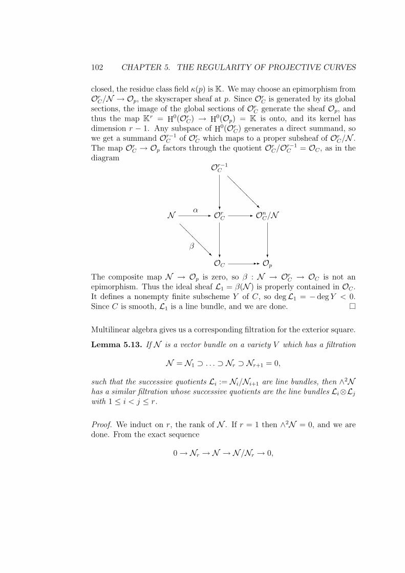
102 CHAPTER 5. THE REGULARITY OF PROJECTIVE CURVES
closed, the residue class field κ(p) is K. We may choose an epimorphism fromOrC/N → Op, the skyscraper sheaf at p. Since Or
C is generated by its globalsections, the image of the global sections of Or
C generate the sheaf Op, andthus the map Kr = H0(Or
C) → H0(Op) = K is onto, and its kernel hasdimension r − 1. Any subspace of H0(Or
C) generates a direct summand, sowe get a summand Or−1
C of OrC which maps to a proper subsheaf of Or
C/N .The map Or
C → Op factors through the quotient OrC/Or−1
C = OC , as in thediagram
Or−1C
@@
@@
@R
Nα
- OrC
?- On
C/N@
@@
@@
βR
OC
?-- Op
?
The composite map N → Op is zero, so β : N → OrC → OC is not an
epimorphism. Thus the ideal sheaf L1 = β(N ) is properly contained in OC .It defines a nonempty finite subscheme Y of C, so degL1 = − deg Y < 0.Since C is smooth, L1 is a line bundle, and we are done.
Multilinear algebra gives us a corresponding filtration for the exterior square.
Lemma 5.13. If N is a vector bundle on a variety V which has a filtration
N = N1 ⊃ . . . ⊃ Nr ⊃ Nr+1 = 0,
such that the successive quotients Li := Ni/Ni+1 are line bundles, then ∧2Nhas a similar filtration whose successive quotients are the line bundles Li⊗Ljwith 1 ≤ i < j ≤ r.
Proof. We induct on r, the rank of N . If r = 1 then ∧2N = 0, and we aredone. From the exact sequence
0 → Nr → N → N /Nr → 0,

5B. PROOF OF THEOREM 5.1 103
and the right exactness of the exterior algebra functor we deduce that
∧(N/Nr) = ∧N/(Nr ∧ (∧N ))
as graded algebras. In degree 2 this gives a right exact sequence
(N/Nr)⊗Nr → ∧2N → ∧2(N/Nr) → 0.
In this case the left hand arrow is a monomorphism because
rank(N/(Nr ⊗Nr)) = (r − 1) · 1 = r − 1
is the same as the difference of the ranks of the right hand bundles,
r − 1 =
(r
2
)−(r − 1
2
).
Thus we can construct a filtration of ∧2N by combining a filtration of(N/Nr)⊗Nr with a filtration of ∧2(N/Nr). The sub-bundles (Ni/Nr)⊗Nr ⊂(N/Nr)⊗Nr give a filtration ofN/Nr with successive quotients Li⊗Lr = Nr
for i < r. By induction on the rank of N , the bundle ∧2(N/Nr), it too hasa filtration with subquotients Li ⊗ Lj, completing the argument.
5B.5 General line bundles
To complete the proof of Theorem 5.1 we will use a general result about linebundles on curves:
Proposition 5.14. Let C be a smooth curve of genus g over an algebraicallyclosed field. If B is a general line bundle of degree ≥ g − 1 then h1 B = 0.
To understand the statement, the reader needs to know that the set Picd(C)of isomorphism classes of line bundles of degree d on C form an irreduciblevariety, called the Picard variety. The statement of the proposition is short-hand for the statement that the set of line bundles B of degree g − 1 thathave vanishing cohomology is an open dense subset of this variety.
We will need this Proposition and more related results in Chapter 8, Lemma8.5 and we postpone the proof until then.

104 CHAPTER 5. THE REGULARITY OF PROJECTIVE CURVES
Proof of Theorem 5.1. Since it does not change the regularity, we may extendthe ground field and assume that K is algebraically closed (the hypothesisthat X is absolutely reduced and irreducible means exactly that X staysreduced and irreducible after this extension.) Set d = degX. By Propositions5.11 and 5.13 the bundle ∧2π∗M can be filtered in such a way that thesuccessive quotients are the tensor products Li ⊗ Lj of two negative linebundles.
Thus to achieve the vanishing of H1(∧2M⊗A) it suffices to chooseA such that
h1(Li⊗Lj⊗A) = 0 for all i, j. By Proposition 5.14, it is enough to choose Ageneral and of degree e such that deg(Li⊗Lj⊗A) = degLi+degLj+e ≥ g−1for every i and j.
Again by Proposition 5.11 we have −d = deg π∗M =∑i degLi. Since the
degLi are negative integers,
degLi + degLj = −d −∑k 6=i,j degLk ≥ −d − r + 2 and it suffices to take
e = g − 1 + d− r + 2. In sum, we have shown that if A is general of degreeg − 1 + d − r + 2 then reg IX ≤ h0A. By the Riemann-Roch theorem wehave h0A = h1A + d− r + 2. By Proposition 5.2, d ≥ r, so degA ≥ g + 1,and Proposition 5.14 implies that h1A = 0. Thus reg IX ≤ h0A = d− r+2,completing the proof.
As we shall see in the next chapter, the bound we have obtained is sometimesoptimal. But the examples that we know in which this happens are of lowgenus; rational and elliptic curves. Are their better bounds for higher genus?At any rate, we shall see in Corollary 8.2 that there are much better boundsfor curves embedded by complete series of high degree. (Exercise 8.4 gives aweak form of this for varieties, even schemes, of any dimension.)
5C Exercises
1. Show that if the curve X ⊂ Pr has an n-secant line (that is, a line thatmeets the curve in n points) then reg IX ≥ n. Deduce that that thereare nondegenerate smooth rational curves X in P3 of any degree d ≥ 3with regSX = degX − codimX. (Hint: consider curves on quadricsurfaces.)

5C. EXERCISES 105
2. Show that if X is the union of 2 disjoint lines in P3, or a conic containedin a plane in P3, then then 2 = reg IX > degX − codimX + 1
3. Show that if Xd is the scheme in P3 given by the equations
x20, x0x1, x
21, x0x
d2 − x1x
d3
then Xd is 1-dimensional, irreducible, and not contained in a hyper-plane. Show that the degree of Xd is 2 but the regularity of SXd
is ≥ d.(In case K is the field of complex numbers, the scheme Xd can be visu-alized as follows: It lies in the first infinitesimal neighborhood, definedby the ideal (x2
0, x0x1, x21) of the line X defined by x0 = x1 = 0, which
has affine coordinate x2/x3. In this sense Xd can be thought of as asubscheme of the normal bundle of X in P3. Identifying the normalbundle with X ×K2 the scheme Xd meets each p×K2 = K2 as a linethrough the origin of K2, and is identified by its slope x0/x1 = (x2/x3)
d.Thus for example if we restrict to values of x2/x3 in the unit circle, wesee that Xd is a ribbon with d twists as in Figure ***((now fig 14)).
((Figure 14))
4. Consider the reduced irreducible 1-dimensional subscheme X of thereal projective space P3
R defined by the equations
x20 − x2
1, x22 − x2
3, x3x0 − x1x2, x0x2 − x1x3
Show that degX = 2 and regSX > degX − codimX, so that theconclusion of Theorem 5.1 does not hold for X. Show that after aground field extension X becomes the union of two disjoint lines.
5. Show that Proposition 5.6 is only true on the sheaf level; the ith syzygymodule of K itself is not isomorphic to a twist of the ith exterior power ofthe first one. (Hint: To see this just consider the number of generatorsof each module, which can be deduced from Nakayama’s Lemma andthe right exactness of the exterior algebra functor (see [Eisenbud 1995,Proposition A2.1]). On the other hand, Use the argument in the textabove to show that the dual of the ith syzygy is isomorphic to the ith
exterior power of the first syzygy.
6. Generalizing Corollary 5.9, suppose ϕ : F1 → F0 is a map of vectorbundles on Pr with F1 = ⊕n
i=1OPr(−bi) and F0 = ⊕hi=1OPr(−ai). Sup-
pose that min aj < min bj (as would be the case if ϕ were a minimal

106 CHAPTER 5. THE REGULARITY OF PROJECTIVE CURVES
presentation of a coherent sheaf.) Show that if the ideal sheaf Ih(ϕ)generated by the h× h minors of ϕ defines a scheme of dimension ≤ 1,then
reg Ih ≤∑
bi −∑
ai − (n− h)(1 + miniai)
7. The monomial curve in Pr with exponents a1 ≤ a2 ≤ · · · ≤ ar is thecurve X ⊂ Pr of degree d = ar parametrized by
φ : P1 3 (s, t) - (sd, sd−a1ta1 , . . . , sd−ar−1tar−1 , td).
Set a0 = 0, and for i = 1, . . . r set αi = ai − ai−1. With notation as inTheorem 5.10, show that
φ∗(M) =⊕i6=j
OP1(−αi − αj).
Now use Theorem 5.10 to show that the regularity of IX is at mostmaxi6=j αi + αj. This exercise is taken from [L′vovsky 1996].

Chapter 6
Linear Series and One-genericMatrices
Revised 8/19/03
In this chapter we will introduce two techniques that are useful for describingthe embeddings of curves and other varieties: linear series, and the 1-genericmatrices to which they give rise. We illustrate these techniques by describingin some detail the free resolutions of ideals of curves of genus 0 and 1 in their“nicest” embeddings.
In the case of genus 0 curves we are looking at embeddings of degree ≥ 1; inthe case of genus 1 curves we are looking at embeddings of degree ≥ 3. Itturns out that the technique of this chapter gives very explicit informationabout the resolutions of ideal of any hyperelliptic curves of any genus gembedded by complete linear series of degree ≥ 2g + 1. We will see inChapter 8 that some qualitative aspects extend to all curves in such “highdegree” embeddings.
For simplicity we suppose throughout this section that K is an algebraicallyclosed field and we work with projective varieties—that is, irreducible alge-braic subsets of a projective space Pr.
107

108 CHAPTER 6. LINEAR SERIES AND ONE-GENERIC MATRICES
6A Rational normal curves
Consider first the plane conics. One such conic—we will call it the standardconic in P2 with respect to coordinates x0, x1, x2—is the curve with equationx0x2 − x2
1 = 0. It is the image of the map
P1 - P2; (s, t) 7→ (s2, st, t2)
Any irreducible conic is obtained from this one by an automorphism—thatis, a linear change of coordinates—of P2.
Analogously, we consider the curve X ∈ Pr that is the image of the map
P1 νr- Pr; (s, t) 7→ (sr, sr−1t, . . . , str−1, tr)
We call X the standard rational normal curve in Pr. By a rational normalcurve in Pr we will mean any curve obtained from this standard one by anautomorphism—a linear change of coordinates—of Pr. Being an image ofP1, a rational normal curve is irreducible. In fact, the map νr is an embed-ding, so X ∼= P1 is a smooth rational (genus 0) curve. Because the mono-mials sr, sr−1t, . . . , tr are linearly independent, it is nondegenerate—that is,not contained in a hyperplane. The intersection of X with the hyperplane∑aixi = 0 is the set of nontrivial solutions of the homogeneous equation∑ais
r−iti. Up to scalars there are (with multiplicity) r such solutions, sothat X has degree r. We will soon see (Theorem 6.8) that any irreducible,nondegenerate curve of degree r in Pr is a rational normal curve in Pr.
In algebraic terms, the standard rational normal curve X is the variety whoseideal is the kernel of the ring homomorphism α : S = K[x0, . . . , xr] → K[s, t]sending xi to sr−iti. Since K[s, t] is a domain, this ideal is prime. Since K[s, t]is generated as a module over the ring α(S) ⊂ K[s, t] by the the finitely manymonomials in K[s, t] of degree < r, we see that dimα(S) = 2. This is thealgebraic counterpart of the statement that X is an irreducible curve.
Note that the defining equation x0x2−x21 of the standard conic can be written
in a simple way as a determinant,
x0x2 − x21 = det
(x0 x1
x1 x2
).
This whole chapter concerns the systematic understanding and exploitationof such determinants!

6A. RATIONAL NORMAL CURVES 109
6A.1 Where’d that matrix come from?
If we replace the variables x0, x1, x2 in the matrix above by their imagess2, st, t2 under ν2 we get the interior of the “multiplication table”
s ts s2 stt st t2
.
The determinant of M goes to zero under the homomorphism α because(s2)(t2) = (st)(st) (associativity and commutativity).
To generalize this to the rational normal curve of degree r we may take anyd with 1 ≤ d < r and write the multiplication table
sr−d sr−d−1t . . . tr−d
sd sr sr−1t . . . sdtr−d
sd−1t sr−1t sr−2t2 . . . sd−1tr−d+1
......
......
...td sr−dtd sr−d−1td+1 . . . tr
and substituting xi for sr−iti we see that the 2 × 2 minors of the (d + 1) ×(r − d+ 1) matrix
Mr,d =
x0 x1 · · · xr−dx1 x2 · · · xr−d+1...
......
...xd xd+1 · · · xr
vanish on X. Arthur Cayley called the matrices Mr,d catalecticant matrices(see Exercises 6.3 and 6.4 for the explanation), and we will follow this ter-minology. They are also called generic Hankel matrices, (a Hankel matrix isany matrix whoses anti-diagonals are constant.)
Generalizing the result that the quadratic form q = detM2,1 generates theideal of the conic in the case r = 2, we now prove:
Proposition 6.1. The ideal I ⊂ S = K[x0, . . . , xr] of the rational normalcurve X ⊂ Pr of degree r is generated by the 2× 2 minors of the matrix
Mr,1 =(x0 · · · xr−1
x1 · · · xr
).

110 CHAPTER 6. LINEAR SERIES AND ONE-GENERIC MATRICES
Proof. Consider the homogeneous coordinate ring SX = S/I which is theimage of the homomorphism
α : S → K[s, t]; xi 7→ sr−iti.
The homogeneous component (S/I)d is equal to K[s, t]rd, which has dimen-sion rd+ 1.
On the other hand, let J ⊂ I be the ideal of 2× 2 minors of Mr,1, so S/I isa homomorphic image of S/J . To prove I = J it thus suffices to show thatdim(S/J)d ≤ rd+ 1 for all d.
We have xixj ≡ xi−1xj+1 mod (J) as long as i − 1 ≥ 0 and j + 1 ≤ r.Thus, modulo J , any monomial of degree d is congruent either to xa0x
d−ar ,
with 0 ≤ a ≤ d, or to xa0xixd−1−ar with 0 ≤ a ≤ d − 1 and 1 ≤ i ≤ r − 1.
There are d + 1 monomials of the first kind and d(r − 1) of the second, sodim(S/J)d ≤ (d+ 1) + d(r − 1) = rd+ 1 as required.
By using the (much harder!) Theorem 5.1 we could have simplified the proofa little: Since the degree of the rational normal curve is r, Theorem 5.1 showsthat reg I ≤ 2, and in particular I is generated by quadratic forms. Thusit suffices to show that, comparing the degree 2 part of J and of I we havedimK J2 ≥ dimK(I)2. This reduces the proof to showing that the minors ofM1,r are linearly independent; one could do this as in the proof above, orusing the result of Exercise 6.8.
Corollary 6.2. The minimal free resolution of the homogeneous coordinatering SX of the rational normal curve X of degree r in Pr is given by theEagon-Northcott complex EN(Mr,1)
0 → (Symr−2 S2)∗ ⊗ ∧rSr → . . .→ (S2)∗ ⊗ ∧3Sr → ∧2Sr
∧2Mr,1- ∧2 S
of the matrix Mr,1 (see Section 11.35). It has Betti diagram of the form
0 1 2 · · · r − 10 1 − − · · · −1 −
(r2
)2(r3
)· · · (r − 1)
(rr
)= r − 1
In particular, SX is a Cohen-Macaulay ring.

6B. 1-GENERIC MATRICES 111
Proof. The codimension of X ⊂ Pr, and thus of I ⊂ S, is r−1, which is equalto the codimension of the ideal of 2×2 minors of a generic 2×r matrix. Thusby Theorem 11.35 the Eagon-Northcott complex is exact. The entries of Mr,1
are of degree 1. From the construction of the Eagon-Northcott complex givenin Section 11H we see that the Betti diagram is as claimed. In particular, theEagon-Northcott complex is minimal. The length of EN(Mr,1) is r − 1, thecodimension of X, so SX is Cohen-Macaulay by the Auslander-BuchsbaumTheorem (11.11).
6B 1-Generic Matrices
To describe some of what is special about the matrices Mr,d we introducesome terminology: IfM is a matrix of linear forms with rows `i = (`i,1, . . . , `i,n)then a generalized row of M is by definition a row∑
i
λi`i = (∑i
λi`i,1, . . . ,∑i
λi`i,n),
that is, a scalar linear combination of the rows of M , with coefficients λi ∈ Kthat are not all zero. We similarly define generalized columns of M . In thesame spirit, a generalized entry of M is a nonzero linear combination ofthe entries of some generalized row of M or, equivalently, a nonzero linearcombination of the entries of some generalized column of M . We will say thatM is 1-generic if every generalized entry of M is nonzero. This is the sameas saying that every generalized row (or column) of M consists of linearlyindependent linear forms.
Proposition 6.3. For each 0 < d < r the matrix Mr,d is 1-generic.
Proof. A nonzero linear combination of the columns of the multiplicationtable corresponds to a nonzero form of degree r−d in s and t, and, similarly,a nonzero linear combination of the rows corresponds to a nonzero form ofdegree d. A generalized entry of Mr,d is the linear form corresponding to aproduct of such nonzero forms, which is again nonzero.
Clearly the same argument would work for a matrix made from part of themultiplication table of any graded domain; we shall further generalize andapply this idea later.

112 CHAPTER 6. LINEAR SERIES AND ONE-GENERIC MATRICES
Determinantal ideals of 1-generic matrices have many remarkable properties.See [Room 1938] for a classical account and [Eisenbud 1988] for a moderntreatment. In particular, they satisfy a generalization of Proposition 6.1 andCorollary 6.2.
Theorem 6.4. If M is a 1-generic matrix of linear forms in S = K[x0, . . . , xr],of size p × q with p ≤ q, over an algebraically closed field K, then theideal Ip(M) generated by the maximal minors of M is prime of codimensionq − p + 1; in particular, its free resolution is given by an Eagon-Northcottcomplex, and S/Ip(M) is a Cohen-Macaulay domain.
Note that q − p + 1 is the codimension of the ideal of p × p minors of thegeneric matrix (Theorem 11.32).
Proof. Set I = Ip(M). We first show that codim I = q−p+1; equivalently, ifX is the projective algebraic set defined by I, we will show that the dimensionof X is r − (q − p + 1). By Theorem 11.32 the codimension of I cannot beany greater than q − p + 1 so, for the codimension statement, it suffices toshow that dimX ≤ r − (q − p+ 1).
Let a ∈ Pr be a point with homogeneous coordinates a0, . . . , ar. The point alies in X if and only if the rows of M become linearly dependent when eval-uated at a. This is equivalent to saying that some generalized row vanishesat a, so X is the union of the zero loci of the generalized rows of M . As M is1-generic, each generalized row has zero locus equal to a linear subspace of Pr
of dimension precisely r− q. A generalized row is determined by an elementof the vector space Kp of linear combinations of rows. Two generalized rowshave the same zero locus if they differ by a scalar, so X is the union of afamily of linear spaces of dimension r−q, parametrized by a projective spacePp−1. Thus dimX ≤ (r − q) + (p− 1) = r − (q − p+ 1).
More formally, we could define X ′ = (y, a) ∈ Pp−1 × Pr | Ry vanishes at awhere Ry denotes the generalized row corresponding to the parameter valuey. The set X ′ fibers over Pp−1 with fibers isomorphic to Pr−q so dimX ′ =(r − q) + (p− 1) = r − (q − p + 1). Also, the projection of X ′ to Pr carriesX ′ onto X, so dimX ≤ dimX ′.
A projective algebraic set, such as X ′, which is fibered over an irreduciblebase with irreducible equidimensional fibers is irreducible ([Eisenbud 1995,

6B. 1-GENERIC MATRICES 113
Exercise 14.3]). It follows that the image X is also irreducible. This provesthat the radical of Ip(M) is prime.
From the codimension statement, and the Cohen-Macaulay property of S, itfollows that the Eagon-Northcott complex associated toM is a free resolutionof S/I, and we see that the projective dimension of S/I is q − p + 1. Bythe Auslander-Buchsbaum Formula (Theorem 11.11) the ring S/I is Cohen-Macaulay.
It remains to show that I itself is prime. From the fact that S/I is Cohen-Macaulay, it follows that all the associated primes of I are minimal, and havecodimension precisely q − p+ 1. Since the radical of I is prime, we see thatin fact I is a primary ideal.
The submatrix M1 of M consisting of the first p− 1 rows is also 1-generic soby what we have already proved, the ideal Ip−1(M1) has codimension q − p.Thus some (p − 1) × (p − 1) minor ∆ of M1 does not vanish identically onX. Since X is the union of the zero loci of the generalized rows of M , thereis even a generalized row whose elements generate an ideal that does notcontain ∆. This generalized row cannot be in the span of the first p− 1 rowsalone, so we may replace the last row of M by this row without changing theideal of minors of M , and we may assume that ∆ /∈ Q := (xp,1, . . . , xp,q). Onthe other hand, since we can expand any p×p minor of M along its last row,we see that I is contained in Q.
Since the ideal Q is generated by a sequence of linear forms, it is prime. Sincewe have seen that I is primary, it suffices to show that ISQ is prime, whereSQ denotes the local ring of S at Q. Since ∆ becomes a unit in SQ we maymake an SQ-linear invertible transformation of the columns of M to bring Minto the form
M ′ =
1 0 . . . 0 | 0 . . . 00 1 . . . 0 | 0 . . . 0. . . . . . . . . . . . | . . . . . . . . .0 0 . . . 1 | 0 . . . 0x′p,1 x′p,2 . . . x′p,p−1 | x′p,p . . . x′p,q
.
where x′p,1, . . . , x′p,q is the result of applying an invertible SQ-linear transfor-
mation to xp,1, . . . , xp,q, and the (p − 1) × (p − 1) matrix in the upper lefthand corner is the identity. It follows that ISQ = (xp,p, . . . , xp,q)SQ.

114 CHAPTER 6. LINEAR SERIES AND ONE-GENERIC MATRICES
Since xp,1, . . . , xp,q are linearly independent moduloQ2SQ, so are x′p,1, . . . , x′p,q.
It follows that SQ/(x′p,p, . . . , x
′p,q) = SQ/ISQ is a regular local ring and thus
a domain (see [Eisenbud 1995, Corollary 10.14]). This shows that ISQ isprime.
Theorem 6.4 can be regarded as a generalization of Proposition 6.1—seeExercise 6.5.
6C Linear Series
We can extend these ideas to give a description of certain embeddings ofgenus 1 curves. At least over the complex numbers, this could be donevery explicitly, replacing monomials by doubly periodic functions. Instead,we approach the problems algebraically, using the general notion of linearseries.
A linear series (L, V, α) on a variety X over K consists of a line bundle Lon X, a finite dimensional K-vector space V and a nonzero homomorphismα : V → H0 L. We define the (projective) dimension of the series to be(dimK V )− 1. The linear series is nondegenerate if α is injective; in this casewe think of V as a subspace of H0(L), and write (L, V ) for the linear series.Frequently we consider a linear series where the space V is the space H0(L)and α is the identity. We call this the complete linear series defined by L,and denote it by |L|.
One can think of a linear series as a family of divisors on X parametrized bythe nonzero elements of V : corresponding to v ∈ V is the divisor which isthe zero locus of the section α(v) ∈ H0(L). Since the divisor correspondingto v is the same as that corresponding to a multiple rv with 0 6= r ∈ K,the family of divisors is really parametrized by the projective space of 1-dimensional subspaces of V , which we think of as the projective space P(V ∗).The simplest kind of linear series is the “hyperplane series” arising from aprojective embedding X ⊂ P(V ). It consists of the family of divisors thatare hyperplane sections of X; more formally this series is (OX(1), V, α) whereOX(1) is the line bundle OP(V )(1) restricted to X and
α : V = H0(OP(V )(1)) → H
0(OX(1))

6C. LINEAR SERIES 115
is the restriction mapping. This series is nondegenerate in the sense above ifand only if X is nondegenerate in P(V ) (that is, X is not contained in anyhyperplane.)
For example, if X ∼= P1 is embedded in Pr as the rational normal curve ofdegree r, then the hyperplane series is the complete linear series
|OP1(r)| = (OP1(r),H0(OP1(r)), id),
where id denotes the identity map.
Not all linear series can be realized as the linear series of all hyperplanesections of an embedded variety. For example, the linear series on P2 ofconics through p. It is defined as follows: Let L = OP2(2). The global sectionsof L correspond to quadratic forms in 3 variables. Taking coordinates x, y, z,we choose p to be the point (0, 0, 1), and we take V to be the vector spaceof quadratic forms vanishing at p, that is, V = 〈x2, xy, xz, y2, yz〉.
In general we define a base-point of a linear series to be a point in the zeroloci of all the sections in α(V ) ⊂ H0(L). Equivalently, this is a point at whichthe sections of α(V ) fail to generate L; or, again, it is a point contained in allthe divisors in the series. In the example above, p is the only base point. Thelinear series is called base point free if it has no base points. The hyperplaneseries of any variety in Pr is base point free because there is a hyperplanemissing any given point.
Recall that a rational map from a variety X to a variety Y is a morphismdefined on an open dense subset U ⊂ X. A nontrivial linear series L =(L, V, α) gives rise to a rational map from X to P(V ) as follows. Let Ube the set of points of X that are not base points of the series, and letΦL : U → P(V ) be the map associating a point p to the hyperplane in V ofsections v ∈ V such that α(v)(p) = 0. If L is base point free then it definesa morphism on all of X.
To express these things in coordinates, choose a basis x0, . . . , xr of V andregard the xi as homogeneous coordinates on P(V ) ∼= Pr. Given q ∈ X,suppose that the global section α(xj) generates L locally near q. There is amorphism from the open set Uj ⊂ X where α(xj) 6= 0 to the open set xj 6= 0in P(V ) corresponding to the ring homomorphism K[x0/xj, . . . , xr/xj] →OX(U) sending xi/xj 7→ ϕ(xi)/ϕ(xj). These morphisms glue together toform a morphism, from X minus the base point locus of L, to P(V ). See

116 CHAPTER 6. LINEAR SERIES AND ONE-GENERIC MATRICES
[Hartshorne 1977, Section 2.7] or [Eisenbud and Harris 2000, Section 3.2.5]for more details.
For example, we could have defined a rational normal curve in Pr to be theimage of P1 by the complete linear series |OP1(r)| = (OP1(r),H0(OP1(r)), id)together with an identification of Pr and P(V )—that is, a choice of basis ofV .
On the other hand, the series of plane conics with a base point at p =(0, 0, 1) above corresponds to the rational map from P2 to P4 sending a point(a, b, c) other than p to (a2, ab, ac, b2, bc). This map cannot be extended to amorphism on all of P2.
If Λ ⊂ Ps is a linear space of codimension r+1, then the linear projection πΛ
from Ps to Pr with center Λ is the rational map from Ps to Pr correspond-ing to the linear series of hyperplanes in Ps containing Λ. Embeddings bycomplete series are simply those not obtained in a nontrivial way by linearprojection.
Proposition 6.5. Let L = (L, V, α) be a base point free linear series ona variety X. The linear series L is nondegenerate (that is, the map α isinjective) if and only if φL(X) ⊂ P(V ) is nondegenerate. The map α issurjective if and only if φL does not factor as the composition of a morphismfrom X to a nondegenerate variety in a projective space Ps and a linearprojection πΛ, where Λ is a linear space not meeting the image of X in Ps.
Proof. A linear form on P(V ) that vanishes on φL(X) is precisely an elementof kerα, which proves the first statement. For the second, note that if φLfactors through a morphism ψ : X → Ps and a linear projection πΛ toPr, where Λ does not meet ψ(X), then the pull back of OPr to ψ(X) isOPs(1)|ψ(X), so ψ∗(OPs(1)) = φ∗L(OPr(1)) = L. If ψ(X) is nondegenerate,then H0(L) is at least (s+ 1)-dimensional, so α cannot be onto. Converselyif α is not onto, we can obtain a factorization as above where ψ is defined bythe complete linear series |L|. The plane Λ is defined by the vanishing of allthe forms in α(V ), and does not meet X because L is base point free.
In case α is a surjection we say that the linear series (L, V, α) is linearly nor-mal. In Corollary 10.13 it is shown that if X ⊂ Pr is a variety then the homo-geneous coordinate ring SX has depth 2 if and only if SX → ⊕d∈Z H0(OX(d))

6C. LINEAR SERIES 117
is an isormorphism. We can restate this condition by saying that, for everyd, the linear series (OX(d),H0(OPr(d)), αd) is complete, where
αd : H0(OPr(d)) → H
0(OX(d))
is the restriction map.
Using Theorem 11.19 we see that ifX is normal and of dimension≥ 1 (so thatSX is locally normal at any homogeneous ideal except the irrelevant ideal,which has codimension ≥ 2), then this condition is equivalent to saying thatSX is a normal ring. In this case the condition that X ⊂ Pr is linearly normalis the “degree 1 part” of the condition for the normality of SX .
6C.1 Ampleness
The linear series that interest us the most are those that provide embeddings.In general, a line bundle L is called very ample if |L| is base point free and themorphism corresponding to |L| is an embedding of X in the projective spaceP(H0(L)). (The term ample is used for a line bundle for which some power isvery ample.) In case X is a nonsingular variety over an algebraically closedfield there is a simple criterion, which we recall here in the case of curvesfrom [Hartshorne 1977, IV, 3.1.(b)].
Theorem 6.6. Let X be a nonsingular curve over an algebraically closedfield. A line bundle L on X is very ample if and only if
h0(L(−p− q)) = h0(L)− 2
for every pair of points p, q ∈ X.
That is: L is very ample if and only if any two points of X (possibly equalto one another) impose independent conditions on the complete series |L|.
Combining this theorem with the Riemann-Roch formula, we easily provethat any line bundle of high degree is very ample. In what follows we writeL(D), where D is a divisor, for the line bundle L ⊗OX(D).
Corollary 6.7. If X is a curve of genus g, then any line bundle of degree≥ 2g + 1 on X is very ample. If g = 0 or g = 1, then the converse is alsotrue.

118 CHAPTER 6. LINEAR SERIES AND ONE-GENERIC MATRICES
Proof. For any points p, q ∈ X, degL(−p− q) > 2g − 2 = degωX , so L andL(−p− q) are both nonspecial. Applying the Riemann Roch formula to eachof these bundles we get
h0(L(−p− q)) = degL − 2− g + 1 = h
0(L)− 2.
as reqired by Theorem 6.6.
Any very ample line bundle must have positive degree, so the converse isimmediate for g = 0. For g = 1, we note that, by Riemann-Roch, h0(L) =degL as long as L has positive degree. Thus a linear series of degree 1 mustmap X to a point, and a linear series of degree 2 can at best map X to P1.Since X 6= P1, such a map is not very ample.
The language of linear series is convenient for proving the following charac-terization:
Theorem 6.8. If X ⊂ Pr is a nondegenerate irreducible curve of degree rthen X is a rational normal curve.
Proof. Suppose that the embedding is given by the linear series L = (L, V, α)on the curve X, so that L is the restriction to X of OPr(1) and degL = r.As X is nondegenerate, Lemma 6.5 shows that h0(L) ≥ r + 1.
We first prove that the existence of a line bundle L on X with degL ≥ 1and h0(L) ≥ 1 + degL implies that X ∼= P1. To see this we do induction ondegL.
If degL = 1 then for any points p, q ∈ X we have degL(−p−q) = −1 whence
h0(L(−p−q)) = 0 ≤ h0(L)−2. In fact, we must have equality, since vanishingat 2 points can impose at most two independent linear conditions. Thus Lis very ample and provides a degree 1 morphism—that is, an isomorphism—from X to P1.
If, on the other hand, degL > 1 then we choose a nonsingular point p ofX. Since the condition of vanishing at p is (at most) one linear conditionon the sections of L, we see that L(−p) has degL(−p) = degL − 1 and
h0(L(−p)) ≥ h0(L)− 1, so L(−p) satisfies the same hypotheses as L.
Since X ∼= P1, and there is only one line bundle on P1 of each degree,L ∼= OP1(d), with d = degL. It follows that h0(L) = 1 + degL. Thus the

6C. LINEAR SERIES 119
embedding is given by the complete linear series, and X is a rational normalcurve.
Corollary 6.9. a) If X is a nondegenerate curve of degree r in Pr, then theideal of X is generated by the 2 × 2 minors of a 1-generic, 2 × r matrix oflinear forms and the minimal free resolution of SX is the Eagon-Northcottcomplex of this matrix. In particular, SX is Cohen-Macaulay.
b) Conversely, if M is a 1-generic 2 × r matrix of linear forms in r + 1variables, then the 2× 2 minors of M generate the ideal of a rational normalcurve.
Proof. a) By Theorem 6.8, a nondegenerate curve of degree r in Pr is, upto change of coordinates, the standard rational normal curve. The desiredmatrix and resolution can be obtained by applying the same change of coor-dinates to the matrix Mr,1.
b) By Theorem 6.4 the ideal P of minors is prime of codimension r − 1,and thus defines a nondegenerate irreducible curve C in Pr. Its resolution isthe Eagon-Northcott complex, as would be the case for the ideal defining thestandard rational normal curve X. Since the Hilbert polynomials of C and Xcan be computed from their graded Betti numbers, these Hilbert polynomialsare equal; in particular C has the same degree, r, as X, and Theorem 6.8completes the proof.
6C.2 Matrices from pairs of linear series.
We have seen that the matrices produced from the multiplication table ofthe ring K[s, t] play a major role in the theory of the rational normal curve.Using linear series we can extend this idea to more general varieties.
Suppose that X ⊂ Pr is a variety embedded by the complete linear series|L| corresponding to some line bundle L. Set V = H0(L), the space oflinear forms on Pr. Suppose that we can factorize L as L = L1 ⊗ L2 forsome line bundles L1 and L2. Choose ordered bases y1 . . . ym ∈ H0(L1) andz1 . . . zn ∈ H0(L2), and let
M(L1,L2)

120 CHAPTER 6. LINEAR SERIES AND ONE-GENERIC MATRICES
be the matrix of linear forms on P(V ) whose (i, j) element is the sectionyi ⊗ zj ∈ V = H0(L). (Of course this matrix is only interesting when it hasat least two rows and two columns, that is, h0 L1 ≥ 2 and h0 L2 ≥ 2.) Eachgeneralized row of M(L1,L2) has entries y ⊗ z1, . . . , y ⊗ zn for some section0 6= y ∈ H0(L1), and a generalized entry of this row will have the form y ⊗ zfor some section 0 6= z ∈ H0(L2).
Proposition 6.10. If X is a variety, and L1,L2 are line bundles on X, thenthe matrix M(L1,L2) is 1-generic, and its 2× 2 minors vanish on X.
Proof. With notation as above, a generalized element of M may be writtenx = y ⊗ z where y, z are sections of L1,L2 respectively. If p ∈ X we mayidentify L1 and L2 with OX in a neighborhood of p and write x = yz. SinceOX,p is an integral domain, x vanishes at p if and only if at least one of yand z vanish at p. Since X is irreducible, X is not the union of the zero lociof a nonzero y and a nonzero z, so no section y ⊗ z can vanish identically.This shows that M is 1-generic. On the other hand, any 2 × 2 minor of Mmay be written as
(y ⊗ z)(y′ ⊗ z′)− (y ⊗ z′)(y′ ⊗ z) ∈ H0(L)
for sections y, y′ ∈ H0(L1) and z, z′ ∈ H0(L2). Locally near a point p of X wemay identify L1,L2 and L with OX,p and this expression becomes (yz)(y′z′)−(yz′)(y′z) which is 0 because OX,p is commutative and associative.
It seems that if both the line bundles L1 and L2 are “sufficiently posi-tive” then the homogeneous ideal of X is generated by the 2 × 2 minorsof M(L1,L2). For example, we have seen that in the case where X is P1 itsuffices that the bundles each have degree ≥ 1. For an easy example general-izing the case of rational normal curves see Exercise 6.11; for more results inthis direction see [Eisenbud et al. 1988]. For less positive bundles, the 2× 2minors of M(L1,L2) may still define an interesting variety containing X, asin Section 6D.
Using the idea introduced in the proof of Theorem 6.4 we can describe thegeometry of the locus defined by the maximal minors of M(L1,L2) in moredetail. Interchanging L1 and L2 if necessary we may suppose that n = h0L2 >
h0 L1 = m so M(L1,L2) has more columns than rows. If y =∑riyi ∈ H0(L1)
is a section, we write `y for the generalized row indexed by y. The maximal

6C. LINEAR SERIES 121
minors of M(L1,L2) vanish at a point p ∈ Pr if and only if some row `yconsists of linear forms vanishing at p; that is,
V (Im(M(L1,L2)) =⋃y
V (`y).
The important point is that we can identify the linear spaces V (`y) geomet-rically.
Proposition 6.11. Suppose X ⊂ Pr is embedded by a complete linear series,and assume that the hyperplane bundle L = OX(1) decomposes as the tensorproduct of two line bundles, L = L1 ⊗ L2. For each y ∈ H0L1 we haveV (`y) = Dy, the projective plane spanned by the divisor Dy ⊂ X defined bythe vanishing of y.
Proof. The linear span of Dy is the interesection of all the hyperplanes con-taining Dy, so we must show that the linear forms appearing in the row `yspan the space of all linear forms vanishing on Dy. It is clear that everyentry y ⊗ zi of this row does in fact vanish where y vanishes, so it suffices toshow that if x ∈ H0 L is a linear form vanishing on Dy then x has the formy⊗ z for some z ∈ H0 L2. Write Dx, Dy for the divisors on X defined by thevanishing of x and y respectively.
There is an exact sequence
0 - L−11
y- OX- ODy
- 0.
Tensoring with L we see that y : L2 → L is the kernel of the restriction mapL → LDy = L ⊗ ODy . Since the section x of L vanishes on Dy, the mapOX → L sending 1 to x factors through a map OX → L2. The image of 1 isthe desired section z.
OX
@@
@@
@
x
R
0 - L2
z
?- L - L|Dy
((Silvio, the vertical map should be a dotted arrow.))

122 CHAPTER 6. LINEAR SERIES AND ONE-GENERIC MATRICES
Note that V (`y) and Dy do not change if we change y by a nonzero scalarmultiple. Thus when we write Dy we may think of y as an element of Pm−1.We can summarize the results of this section, in their most important specialcase, as follows.
Corollary 6.12. Suppose that X ⊂ Pr is embedded by the complete linearseries |L|, and that L1,L2 are line bundles on X such that L = L1 ⊗ L2.Suppose that h0 L1 = m ≤ h0 L2. If y ∈ H0 L1, write Dy for the correspondingdivisor. If Dy denotes the linear span of Dy, then the variety defined by themaximal minors of M(L1,L2) is
Y = V (Im(M(L1,L2))) =⋃
y∈Pm−1
Dy.
We may illustrate Corollary 6.12 with the example of the rational normalcurve. Let X = P1 and let L1 = OP1(1),L2 = OP1(r − 1) so that
M(L1,L2) = Mr,1 =(x0 x1 . . . xr−1
x1 x2 . . . xr.
)
The generalized row corresponding to an element y = (y1, y2) ∈ P1 has theform
`y = (y0x0 + y1x1, y0x1 + y1x2, · · · , y0xr−1 + y1xr).
The linear space V (`y) is thus the set of solutions of the linear equations
y0x0 + y1x1 = 0y0x1 + y1x2 = 0...y0xr−1 + y1xr = 0,
Since these r equations are linearly independent, V (`y) is a single point. Solv-ing the equations, we see that this point has coordinates xi = (−y0/y1)
ix0.Taking y0 = 1, x0 = sr, y1 = −s/t we obtain the usual parametrizationxi = sr−iti of the rational normal curve.

6C. LINEAR SERIES 123
6C.3 Linear subcomplexes and mapping cones
We have seen that if X is embedded by the complete linear series |L| and ifL = L1⊗L2 is a factorization, then by Theorem 6.4 and Proposition 6.10 theideal I = IX of X contains the ideal of 2× 2 minors of the 1-generic matrixM = M(L1,L2). This has an important consequence for the free resolutionof M .
Proposition 6.13. Suppose that X ⊂ Pr is a variety embedded by a completelinear series |L|, and that L = L1⊗L2 for some line bundles L1,L2 on X. LetM ′ be a 2× h0(L2) submatrix of M(L1,L2), and let J be the ideal generatedby the 2×2 minors of M ′. If F : · · · → F0 → IX is a minimal free resolutionand E : · · · → E0 → J denotes the Eagon-Northcott complex of M ′, then Eis a subcomplex of F in such a way that Fi = Ei ⊕Gi for every i.
Proof. Choose any map α : E → F lifting the inclusion J ⊂ I = IX . Wewill show by induction that αi : Ei → Fi is a split inclusion for every i ≥ 0.Write δ for the differentials—both of E and of F. Write P = (x0, . . . , xr) forthe homogeneous maximal ideal of S. It suffices to show that if e ∈ Ei bute /∈ PEi (so that e is a minimal generator) then αi(e) /∈ PFi.
Suppose on the contrary αie ∈ PFi. In the case i = 0, we see that δe mustbe in PI ∩ J . But the Eagon-Northcott complex EN(M ′) is a minimal freeresolution, so δe is a nonzero quadratic form. As X is nondegenerate theideal I = IX does not contain any linear form, so we cannot have e ∈ PI.
Now suppose i > 0, and assume by induction that αi−1 maps Ei−1 isomorphi-cally to a summand of Fi−1. Since F is a minimal free resolution the relationαi ∈ PFi implies that
αi−1δe = δαie ∈ P 2Fi−1.
However, the coefficients in the differential of the Eagon-Northcott complexare all linear forms. As EN(M ′) is a minimal free resolution we have δe 6= 0,so δe /∈ P 2Ei−1, a contradiction since Ei−1 is mapped by αi−1 isomorphicallyto a summand of Fi−1.
The reader may verify that the idea used in this proof applies more generallywhen one has a linear complex that is minimal in an appropriate sense and

124 CHAPTER 6. LINEAR SERIES AND ONE-GENERIC MATRICES
maps to the “least degree part” of a free resolution. We will study linearcomplexes further in the next chapter.
Proposition 6.13 is typically applied when L1 has just two sections—otherwise,to choose the 2×n submatrix M ′ one effectively throws away some sections,losing some information. It would be very interesting to have a systematicway of exploiting the existence of further sections, or more generally of ex-ploiting the presence of many difference choices of factorization L = L1⊗L2
with a choice of two sections of L1. In the next section we will see a casewhere we have in fact many such factorizations, but our analysis ignores thefact. See, however, Kempf [Kempf 1989] for an interesting case where thepresence of multiple factorizations is successfully exploited.
The situation produced by Proposition 6.13 allows us to split the analysis ofthe resolution into two parts. Here is the general setup, which we will applyto a certain family of curves in the next section.
Proposition 6.14. Suppose that F : · · · → F0 is a free complex, with freesubcomplex E : · · · → E0. If Ei is a summand of Fi for every i and wewrite Fi = Gi ⊕ Ei then G = F/E : · · · → G0 is again a free complex and,then F is the mapping cone of the map α : G[−1] → E defined by takingαi : Gi+1 → Ei to be the composite
Gi+1 ⊂ Gi+1 ⊕ Ei+1 = Fi+1δ- Fi = Gi ⊕ Ei - Ei,
where δ is the differential of the complex F.
Proof. Immediate from the definitions.
To reverse the process and construct F as a mapping cone, we need a differentway of specifying the map from G[−1] to E. In our situation the followingobservation is convenient. We leave to the reader the easy formalization forthe most general case.
Proposition 6.15. Suppose that J ⊂ I are ideals of S. Let G : · · · → G0
be a free resolution of I/J as an S-module. Let E : · · · → E1 → S be a freeresolution of S/J . If α : G → E is a map of complexes lifting the inclusionI/J → S/J , then the mapping cone, F, of α is a free resolution of S/I.If matrices representing the maps αi : Gi → Ei have all nonzero entries of

6D. ELLIPTIC NORMAL CURVES 125
positive degree, and if both E and G are minimal resolutions, then F is alsoa minimal resolution.
Proof. Denoting the mapping cylinder of α by F, we have an exact sequence0 → E → F → G[−1] → 0. Since G and E have no homology except atthe right hand end, we see from the long exact sequence in homology that
HiF = 0 for i ≥ 2. From the end of the sequence we get
· · · → H1 E → H1 F → I/J → S/J → H0 F → 0,
where the map I/J → S/J is the inclusion. It follows that H1 F = 0 andF : · · · → F1 → S = F0 is a resolution of S/I.
6D Elliptic normal curves
Let X be a nonsingular, irreducible curve of genus 1, let L be a very ampleline bundle on X, and let d be the degree of L. By Corollary 6.7, d ≥ 3,and by the Riemann-Roch formula, h0(L) = d. Thus the complete linearseries |L| embeds X as a curve of degree d in Pr = Pd−1. We will call suchan embedded curve an elliptic normal curve of degree d. (Strictly speaking,an elliptic curve is a nonsingular projective curve of genus 1 with a chosenpoint, made into an algebraic group in such a way that the chosen point isthe origin. We will not need the chosen point for what we are doing, andwe will accordingly not distinguish between an elliptic curve and a curve ofgenus 1.)
In this section we will use the ideas introduced above to study the minimalfree resolution F of SX , where X ⊂ Pr is an elliptic normal curve of degreed. Specifically, we will show that F is built up as a mapping cone from anEagon-Northcott complex E and its dual, appropriately shifted and twisted.Further, we shall see that SX is always Cohen-Macaulay, and of regularity 3.
The cases with d ≤ 4 are easy and somewhat degenerate, so we will dealwith them separately. If d = 3, then X is embedded as a cubic in P2, so the

126 CHAPTER 6. LINEAR SERIES AND ONE-GENERIC MATRICES
resolution has Betti diagram
0 10 1 −1 − −2 − 1
In this case the Eagon-Northcott complex in question would be that of the2× 2 minors of a 2× 1 matrix—and thus isn’t visible at all.
Next suppose d = 4. By the Riemann-Roch formula h0(L2) = 8 − g + 1 =8, while, since r = 3, the space of quadratic forms on Pr has dimensiondimS2 = 10. It follows that the ideal IX of X contains at least 2 linearlyindependant quadratic forms, Q1, Q2. If Q1 were reducible then the quadricit defines would be the union of two planes. Since X is irreducible, X wouldhave to lie entirely on one of them. But by hypothesis X is embedded bythe complete series |L|, so X is nondegenerate in P3. Thus Q1 is irreducible,and S/(Q1) is a domain.
It follows that Q1, Q2 form a regular sequence. The complete intersectionof the two quadrics corresponding to Q1 and Q2 has degree 4 by Bezout’sTheorem, and it contains the degree 4 curve X, so it is equal to X. Sinceany complete intersection is unmixed (see Theorem 11.23), the ideal IX isequal to (Q1, Q2). Since these forms are relatively prime, the free resolutionof SX has the form
0 - S(−4)
(Q2
−Q1
)- S2(−2)
(Q1, Q2 )- S,
with Betti diagram0 1 2
0 1 −1 − 2 −2 − − 1
In this case the Eagon-Northcott complex in question is that of the 2 × 2minors of a 2× 2 matrix. It has the form
0 - S(−2)Q1- S.
In both these cases, the reader can see from the Betti diagrams that SX isCohen-Macaulay of regularity 3 as promised.

6D. ELLIPTIC NORMAL CURVES 127
Henceforward, we will freely assume that d ≥ 5 whenever it makes a differ-ence. LetD be a divisor consisting of 2 points onX. We have h0(OX(D)) = 2and h0(L(−D)) = d − 2, so from the theory of the previous section we seethat M = M(OX(D),L(−D)) is a 2 × (d − 2) matrix of linear forms on Pr
that is 1-generic, and the ideal J of 2 × 2 minors of M is contained in theideal of X. Moreover, we know from Theorem 6.4 that J is a prime idealof codimension equal to (d − 2) − 2 + 1 = r − 2; that is, J = IY is thehomogeneous ideal of an irreducible surface Y containing X. The surface Yis the union of the lines spanned by the divisors linearly equivalent to D inX. Since Y is a surface, X is a divisor on Y .
We can now apply Proposition 6.13 and Proposition 6.15 to construct the freeresolution of I from the Eagon-Northcott resolution of J and a resolution ofI/J . To this end we must identify I/J . We will show that it is a line bundleon Y .
To continue our analysis, it is helpful to identify the surface Y . Althoughit is not hard to perform this analysis in general, the situation is slightlysimpler when D = 2p and L = OX(dp) for some point p ∈ X. This case willsuffice for the analysis of any elliptic normal curve because of the following:
Theorem 6.16. If L is a line bundle of degree k on a smooth projective curveof genus 1 over an algebraically closed field, then L = OX(kp) for some pointp ∈ X.
Proof. The result follows from simple facts about the group law on X: Wemay choose a point q ∈ X, and regard X as an algebraic group with originq. There is a one-to-one correspondence between points of X and divisorsof degree 0 taking a point p to the divisor p − q; if D is a divisor of degree0 then, by the Riemann-Roch theorem, the line bundle OX(D + q) has aunique section σ. It vanishes at the unique point p for which p ∼ D + q,that is p − q ∼ D. It follows from the definition of the group law that thiscorrespondence is an isomorphism of groups.
Multiplication by k is a nonconstant map of projective curves X → X,and is thus surjective. It follows that there is a divisor p − q such thatD − kq ∼ k(p− q), and thus D ∼ kp as claimed.
Returning to our elliptic normal curve X embedded by |L|, we see from

128 CHAPTER 6. LINEAR SERIES AND ONE-GENERIC MATRICES
Theorem 6.16 that we may write L = OX(dp) for some p ∈ X, and wechoose D = 2p. To make the matrix M(OX(2p),OX((d − 2)p)) explicit, wemust choose bases of the global sections of OX(dp) and OX(2p).
In general the global sections of OX(kp) may be thought of as rational func-tions on X having no poles except at p, and a pole of order at most k at p.Thus there is a sequence of inclusions
K = H0OX ⊆ H0OX(p) ⊆ H0OX(2p) ⊆ . . . ⊆ H0OX(kp) ⊆ . . . .
Moreover, we have seen that h0OX(kP ) = k for k ≥ 1. It follows that1 ∈ H0(OX) = H0(OX(p) may be considered as a basis of either of thesespaces. But there is a new section σ ∈ H0(OX(2p)), with a pole at p of orderexactly 2, and in addition to 1 and σ a section τ ∈ H0(OX(3p)) with orderexactly 3. The function σ2 has a pole of order 4, and continuing in this waywe get:
Proposition 6.17. If p is a point of the smooth projective curve X of genus1 and d ≥ 1 is an integer, then the rational functions σa for 0 ≤ a ≤ d/2and σaτ , for 0 ≤ a ≤ (d− 3)/2, form a basis of H0(OX(d)).
Proof. The function σaτ b has pole of order 2a + 3b at p, so the given func-tions are all sections, and are linearly independent. Since the dimension of
H0(OX(dp)) is d = 1 + bd/2c+ b(d− 1)/2c = (1 + bd/2c) + (1 + b(d− 3)/2c),the number of sections given, this suffices.
Corollary 6.18. Let X be an elliptic curve, and let p ∈ X be a point. Ifd ≥ 2 and e ≥ 3 are integers, then the multiplication map
H0(OX(dp))⊗ H
0(OX(ep)) → H0(OX((d+ e)p)
is surjective. In particular, if L is a line bundle on X of degree ≥ 3, andX ⊂ Pr is embedded by the complete linear series |L|, then SX is Cohen-Macaulay and normal.
Proof. The sections of H0(OX(dp)) exhibited in Proposition 6.17 include sec-tions with every vanishing order at p from 0 to d except for 1, and similarlyfor H0(OX(dp)). When we multiply sections we add their vanishing orders atp, so the image of the multiplication map contains sections with every van-ishing order from 0 to d+ e except 1, a total of d+ e distinct orders. These

6D. ELLIPTIC NORMAL CURVES 129
elements must be linearly independent, so they span the d + e-dimensionalspace H0(OX((d+ e)p).
For the second statement we may first extend the ground field if necessaryuntil it is algebraically closed, and then use Theorem 6.16 to rewrite L asOX(dp) for some d ≥ 3. From the first part of the Corollary we see that themultiplication map
H0OX(d)⊗ H
0OX(md) → H0OX((m+ 1)d)
is surjective for every m ≥ 0. From Corollary 10.13 we see that SX hasdepth 2 (and is even normal). Since SX is a 2-dimensional ring, this impliesin particular that it is Cohen-Macaulay.
For example, consider an elliptic normal cubic X ⊂ P2. By Theorem 6.16 theembedding is by a complete linear series |OX(3p)| for some point p ∈ X. LetS = K[x0, x1, x2] → SX = ⊕n H0(OX(3np) be the map sending x0 7→ 1; x1 7→σ; x2 7→ τ . By Corollary 6.18 this map is a surjection. To find its kernel,the equation of the curve, consider H0(OX(6p)), the first space for which wecan write down an “extra” section τ 2. We see that there must be a linearrelation among 1, σ, σ2, σ3, τ, στ and τ 2, and since σ3 and τ 2 are the only twosections on this list with a triple pole at p, each must appear with a nonzerocoefficient. From this we get an equation of the form τ 2 = f(σ)+τg(σ), wheref is a polynomial of degree 3 and g a polynomial of degree ≤ 1. This is theaffine equation of the embedding of the open subset X \ p of X in A2 withcoordinates σ, τ corresponding to the linear series |OX(3p)|. Homogenizing,we get an equation of the form x0x
22 = F (x0, x1)+x0x2G(x0, x1) where F and
G are the homogenizations of f and g respectively. Since 3p is a hyperplanesection, the point p goes to a flex point of X, and the line at infinity is theflex tangent. When the characteristic of K is not 2 or 3, further simplificationyields the Weierstrass normal form y2 = x3 +ax+ b for the equation in affinecoordinates.
In general, the table giving the multiplication between the sections ofOX(2p),and the sections of OX((d − 2)p), with the choice of bases above, can bewritten, as
1 σ . . . σn−1 τ στ . . . σm−1τ1 1 σ . . . σn−1 τ στ . . . σm−1τσ σ σ2 . . . σn στ σ2τ . . . σmτ,

130 CHAPTER 6. LINEAR SERIES AND ONE-GENERIC MATRICES
where n = bd/2c and m = b(d− 3)/2c so that (m+ 1) + (n+ 1) = r+ 1 = d.Taking xi to be the linear form on Pr corresponding to σi and yj to be thelinear form corresponding to σjτ , the matrix M = M(OX(2p),OX((d− 2)p)takes the form
M =(x0 x1 · · · xn−1
x1 x2 · · · xn| y0 y1 · · · ym−1
y1 y2 · · · ym
)
((Silvio, the vertical line should be the same height at the two rowsof the matrix.)) where the vertical line indicates the division of M intotwo parts, which we will call M ′ and M ′′. The reader should recognize thematrices M ′ and M ′′ from Section 6A: their ideals of 2 × 2 minors definerational normal curvesX ′ andX ′′ of degrees n andm in the disjoint subspacesL′ defined by y0 = · · · = ym and L′′ defined by x0 = · · · = xn respectively.
Let Y be the vanishing locus of the 2 × 2 minors of M , the union of thelinear spaces defined by the vanishing of the generalized rows of M . SinceM is 1-generic each generalized row consists of linearly independent linearforms—that is, its vanishing locus is a line. Moreover, the intersection ofthe line with the subspace Lx is the the point on the rational normal curvein that space given by the vanishing of the corresponding generalized rowof M ′, and similarly for Ly. Thus the matrix M defines an isomorphismα : X ′ → X ′′, and in terms of this isomorphism the surface Y is the unionof the lines joining p ∈ X ′ to α(p) ∈ X ′′. Such a surface is called a rationalnormal scroll; the name is justified by the picture below: ((the picturecould be made nicer with more rolls at the ends))

6D. ELLIPTIC NORMAL CURVES 131
ee /
QQs
Dλ
XXXXXy
X ′ X ′′
Y XXXXz
* QQk
A scroll
((This is picture 15))
In the simplest interesting case, r = 3, we get m = 2 and n = 0 so
M =(x0 x1
x1 x2
).
In this case Y is the cone in P3 over the irreducible conic x0x2 = x21 in P2,
and the lines F are the lines through the vertex on this cone. When r ≥ 4,however, we will show that Y is nonsingular.
Proposition 6.19. Suppose that d ≥ 5, or equivalently that r ≥ 4. Thesurface Y , defined by the 2× 2 minors of the matrix
M = M(OX(2p),OX((d− 2)p),
is nonsingular.
Proof. As we have already seen, Y is the union of the lines defined by thegeneralized rows of the matrix M . To see that no two of these lines canintersect, note that any two distinct generalized rows span the space of allgeneralized rows, and thus any two generalized rows contain linear forms thatspan the space of all linear forms on Pr. It follows that the set on which thelinear forms in both generalized rows vanish is the empty set.
We can parametrize Y on the open set where x0 6= 0 as the image of A2
by the map sending f : (t, u) 7→ (1, t, . . . , tm, u, ut, . . . , utn). The differentialof f is nowhere vanishing, so f is an immersion. It is one-to-one because,
132 CHAPTER 6. LINEAR SERIES AND ONE-GENERIC MATRICES
from our previous argument, the lines t = c1 and t = c2 are distinct for anydistinct constants c1, c2. A similar argument applies to the open set ym 6= 0,and these two sets cover Y .
One can classify the 1-generic matrices of size 2 × m completely using theclassification of matrix pencils due to Kronecker and Weierstrass. The resultshows that the varieties defined by the 2 × 2 minors of such a matrix areall rational normal scrolls of some dimension; for example, if such a varietyis of dimension 1 then it is a rational normal curve. See Eisenbud-Harris[Eisenbud and Harris 1987] for details and many more properties of theseinteresting and ubiquitous varieties.
To identify X as a divisor, we use a description of the Picard group andintersection form of Y .
Proposition 6.20. Let Y be the surface defined in Proposition 6.19. Thedivisor class group of Y is
PicY = ZH ⊕ ZF,
where H is the class of a hyperplane section and F is the class of a linedefined by the vanishing of one of the rows of the matrix M(OX(D),L(−D))used to define Y . The intersection numbers of these classes are F · F = 0,F ·H = 1, and H ·H = r − 1.
Proof. The intersection numbers are easy to compute: We have F · F = 0because two fibers of the map to P1 (defined by the vanishing of the general-ized rows of M) do not meet, and F ·H = 1 because F is a line, which meetsa general hyperplane transversely in a single point. Since Y is a surface thenumber H ·H is just the degree of the surface.
Modulo the polynomial xm+1 − y0 then the matrix M becomes the matrixwhose 2×2 minors define the rational normal curve of degreem+n+2 = r−1.Thus the hyperplane section of Y is this rational normal curve, and the degreeof Y is also r − 1. The fact that the intersection matrix(
0 11 r − 1
)we have just computed has rank 2 shows that the divisor classes of F and Hare linearly independent. The proof that they generate the group is outlinedin Exercise 6.9 [Hartshorne 1977, V.2.3] or [Eisenbud and Harris 1987].
6D. ELLIPTIC NORMAL CURVES 133
We can now identify a divisor by computing its intersection numbers withthe classes H and F :
Proposition 6.21. In the basis introduced above, the divisor class of X onthe surface Y is 2H − (r − 3)F .
Proof. By Proposition 6.20 we can write the class of X as [X] = aH + bFfor some integers a, b. From the form of the intersection matrix we see thata = X.F and b = X.H − (r − 1)a. Since the lines F on the surface are thelinear spans of divisors on X that are linearly equivalent to D, and thus ofdegree 2, we have a = 2. On the other hand X.H is the degree of X as acurve in Pr, that is, r + 1. Thus b = r + 1− (r − 1)2 = −(r − 3).
In general, we see that the sheaf of ideals I/J = IX/Y defining X in Y is thesheaf
I/J = OY ((r − 3)F − 2H) = OY ((r − 3)F )(−2)
and thus the homogeneous ideal I/J of X in Y is, up to a shift of grading,⊕n≥0 H0OY ((r−3)F )(n). Here is a first step toward identifying this module
and its free resolution.
Proposition 6.22. The cokernel K of the matrix
M = M(OX(2p),OX((r − 1)p))
has associated sheaf on Pr equal to K = OY (F ).
Proof. Let K be the sheaf on Pr that is associated to the module K. Wewill first show that K is an invertible sheaf on Y . The entries of the matrixM span all the linear forms on Pr so locally at any point p ∈ Pr one of themis invertible, and we may apply the following result.
Lemma 6.23. If N is a 2×n matrix over a ring R and M has one invertibleentry, then the cokernel of N is isomorphic to R modulo the 2× 2 minors ofN .
Proof. Using row and column operations we may put N into the form
N ′ =(
1 0 . . . 00 r2 . . . rn
)

134 CHAPTER 6. LINEAR SERIES AND ONE-GENERIC MATRICES
for some ri ∈ R. The result is obvious for this N ′, which has the samecokernel and same ideal of minors as N .
Continuing the proof of Proposition 6.22, we note that the module K isgenerated by degree 0 elements e1, e2 with relations xie1 + xi+1e2 = 0 andyie1 + yi+1e2 = 0. The elements ei determine sections σi of K. Thus if p ∈ Yis a point where some linear form in the second row of M is nonzero, then σ1
generates K locally at p. As the second row vanishes precisely on the fiberF , this shows that the zero locus of σ1 is contained in F .
Conversely, suppose p ∈ F so that the second row of M vanishes at p. Sincethe linear forms in M span the space of all linear forms on Pr, one of thelinear forms in the first row of M is nonzero at p. Locally at p this meansm1σ1 + m2σ2 = 0 in Kp where m1 is a unit in OY,p, the local ring of Y atp, and m2 is in the maximal ideal mY,p ⊂ OY,p. Dividing by m1 we see thatσ1 ∈ mY,pKp. Since mY,p is the set of functions vanishing at p, we see that σ1
vanishes at p when considerd as a section of a line bundle. Since this holdsat all p ∈ F we obtain K = OY (F ).
Recall that we wish to find a free resolution (as S-module) of the ideal IX/Y ⊂S/IY , that is, of the module of twisted global sections of the sheaf OY ((r −3)F )(−2). This sheaf is the sheafification of the module K⊗(r−3)(−2), butone can show that for r ≥ 5 this module has depth 0, so it differs from themodule of twisted global sections. A better module—in this case the rightone—is given by the symmetric power.
Proposition 6.24. Let L be an S-module. If the sheaf L = L on Pr is locallygenerated by at most one element, then the sheafification L⊗k of L⊗k is alsothe sheafification of Symk(L). In particular, this is the case when L is a linebundle on some subvariety Y ⊂ Pr.
Proof. Since the formation of tensor powers and symmetric powers commuteswith localization, and with taking degree 0 parts, it suffices to do the casewhere L is a module over a ring R such that L is generated by at most oneelement. In this case, L ∼= R/I for some ideal I. If ri are elements of R/Ithen
r1 ⊗ r2 = r1r2(1⊗ 1) = r2 ⊗ r1 ∈ R/I ⊗R/I.

6D. ELLIPTIC NORMAL CURVES 135
Since Sym2(L) is obtained from L⊗L by factoring out the submodule gener-ated by elements of the form r1⊗ r2− r2⊗ r1, we see that L⊗L = Sym2(L).The same argument works for products with k factors.
We return to the module K = cokerM , and study Symr−3K.
Proposition 6.25. With notation as above, ⊕d H0(L⊗(r−3)(d)) = Symr−3Kas S-modules. Its free resolution is, up to a shift of degree, given by the dualof the Eagon-Northcott complex of M .
Proof. We use the exact sequence of Corollary 10.8,
0 → H0m(Symr−3K) → Symr−3K →
⊕d
H0(L(d)) → H
1m(Symr−3K) → 0.
Thus we want to show that H0m(Symr−3K) = H1
m(Symr−3K) = 0. By Propo-sition 10.12 it suffices to prove that the depth of K is at least 2. Equivalently,by the Auslander-Buchsbaum Formula 11.11 it suffices to show that the pro-jective dimension of Symr−3K is at most r − 1.
From the presentation Sr−1(−1)ϕ- S2 → K → 0, we can derive a presen-
tation
Sr−1 ⊗ Symr−4 S2(−1)
ϕ⊗1- Symr−3 S2 - Symr−3K → 0
(see [Eisenbud 1995, Proposition A2.2.d]). This map is, up to some identifi-cations and a twist, the dual of the last map in the Eagon-Northcott complexassociated to Mµ, namely
0 → (Symr−3S2)∗ ⊗ ∧r−1Sr−1(−r + 1) → (Symr−4S
2)∗ ⊗ ∧r−2Sr−1(−r + 2).
To see this we use the isomorphisms ∧iSr−1 ' (∧r−1−iSr−1)∗ (which dependon an “orientation”, that is, a choice of basis element for ∧r−1Sr−1). Sincethe Eagon-Northcott complex is a free resolution of the Cohen-Macaulay S-module S/I, its dual is again a free resolution, so we see that the moduleSymr−3K is also of projective dimension r − 1.
To sum up: we have shown that there is an S-free resolution of the homo-geneous coordinate ring S/I of the elliptic normal curve X obtained as amapping cone of the Eagon-Northcott complex of the matrix M , which is a

136 CHAPTER 6. LINEAR SERIES AND ONE-GENERIC MATRICES
resolution of J , and the resolution of the module I/J . The proof of Proposi-tion 6.25 shows that the dual of the Eagon-Northcott complex, appropriatelyshifted, is a resolution of Symr−3K, while I/J ∼= Symr−3K(−2). Thus thefree resolution of I/J is isomorphic to the dual of the Eagon-Northcott com-plex with a different shift in degrees. If we choose an orientation as above itmay be written as:
0 → (∧2S2)∗(−r − 1) - (∧2Sr−1)∗(−r + 1) - · · ·
· · · - Sr−1 ⊗ Symr−4 S2(−3)
ϕ⊗1- Symr−3 S2(−2).
So far we have simply applied Proposition 6.15, whose conclusion is that themapping cone is a resolution. But in this case, the resolution is minimal:
Theorem 6.26. The minimal free resolution of an elliptic normal curve inPr has the form
0 - Symr−3(S2)∗ ⊗ ∧r−1Sr−1(−r + 1) - . . .
*
0⊕
* ⊕*
HHHHj∧2(S2)∗(−r − 1) - ∧2(Sr−1)∗(−r + 1) - . . .
. . . - (S2)∗ ⊗ ∧3Sr−1(−3) - ∧2Sr−1(−2)HHHHj
* ⊕* ⊕
S→ SX → 0.
*
. . . - (Sr−1)∗ ⊗ Symr−4 S2(−3) - Symr−3 S
2(−2)
.
((Silvio, let’s talk about how to improve the readability of thisdiagram)) It has Betti diagram of the form
0 1 2 . . . r − 2 r − 10 1 0 0 · · · 0 01 0 b1 b2 . . . br−2 02 0 0 0 . . . 0 1
with
bi = i
(r − 1
i+ 1
)+ (r − i− 1)
(r − 1
i− 1
).
In particular, regX = 3.

6E. EXERCISES 137
Notice that the terms of the resolution are symmetric about the middle. Acloser analysis shows that the i-th map in the resolution can be taken to bethe dual of the (r−1− i)-th map, and if r ∼= 0 (mod 4) then the middle mapcan be chosen to be skew symmetric, while if r ∼= 2 (mod 4) then the middlemap can be chosen to be symmetric. See Eisenbud-Buchsbaum [Buchsbaumand Eisenbud 1977] for the beginning of this theory.
Proof. We have already shown that the given complex is a resolution. Eachmap in the complex goes from a free module generated in one degree to a freemodule generated in a lower degree. Thus the differentials are represented bymatrices of elements of strictly positive degree, and the complex is minimal.Given this, the value for the regularity follows by inspection.
The regularity statement says that for an elliptic normal curve X (degreed = r+1 and codimension c = r−1 in Pr the regularity of the homogeneouscoordinate ring SX is precisely d− c = 2. By the Gruson-Lazarsfeld-PeskineTheorem 5.1, this is the largests possible regularity. In general, ifX is a curveof genus g. We shall see in the next chapter that linearly normal curves ofhigh degree compared to their genus always have regularity 3—which is lessthan the Gruson-Lazarsfeld-Peskine bound when the genus is greater than 1.
The methods used here apply, and give information about the resolution, fora larger class of divisors on rational normal scrolls. The simplest applicationis to give the resolution of the ideal of any set of points lying on a rationalnormal curve in Pr. It also works for high degree embeddings of hyperellip-tic curves (in the sense of Chapter 8, trigonal curves of any genus in theircanonical embeddings, and many other interesting varieties. See [Eisenbud1995, end of appendix A2] for an algebraic treatment with further references.
6E Exercises
1. []The Catalecticant matrix((this is preamble to the next 4 exercises)) (The results of Ex-
ercises 6.2 and 6.3 were proved by a different method, requiring char-acteristic 0, by Gruson-Peskine [Gruson and Peskine 1982], followingthe observation by T. G. Room [Room 1938] that these relations held

138 CHAPTER 6. LINEAR SERIES AND ONE-GENERIC MATRICES
set-theoretically. The simple proof in full generality sketched here wasdiscovered by Conca [Conca 1998].)
2. Prove that Ie(Mr,d) = Ie(Mr,e−1) for all d with e ≤ d+1 and e ≤ r−d+1and thus the ideal Ie(Mr,d) is prime of codimension r−2e+1, with freeresolution given by the Eagon-Northcott complex associated to Mr,e.In particular, the ideal of the rational normal curve may be written asI2(Mr,e) for any e ≤ r − d. You might follow these steps.
(a) Using the fact that Transpose Mr,d = Mr,d+1, reduce the problemto proving Ie(Mr,d) ⊂ Ie(Mr,d+1) for e− 1 ≤ d < d+1 ≤ r− e+1.
(b) If a = (a1, . . . , as) with 0 ≤ a1, . . . , as and b = (b1, . . . , bs) with0 ≤ b1, . . . , bs with ai + bj ≤ r for every i, j, then we write [a, b]for the determinant of the submatrix involving rows a1, . . . , as andcolumns b1, . . . , bs of the triangular array
x0 x1 . . . xr−1 xrx1 x2 . . . xr...
...xr−1 xrxr
.
Let e be the vector of length s equal to (1, . . . , 1). Prove theidentity
[a+ e, b] = [a, b+ e]
whenever this makes sense.
(c) Generalize the previous identity as follows: for I ⊂ 1, . . . , swrite #I for the cardinality of I, and write e(I) for the charac-teristic vector of I, which has a 1 in the i-th place if and only ifi ∈ I. Show that for each k between 1 and s we have∑
#I=k
[a+ e(I), b] =∑
#J=k
[a, b+ e(J)].
(Hint: Expand each minor [a+ e(I), b] on the left hand side alongthe collection of rows indexed by I, as
[a+ e(I), b] =∑
#J=k
(−1)|I|[aI + e(I)I , bJ ][aIc + e(Ic)I , bJc ]

6E. EXERCISES 139
where|I| =
∑i∈I
i,
aI denotes the subvector involving only the indices in I and Ic
denotes the complement of I, etc. Expand the right hand sidesimilarly using along the set of columns from J , and check thatthe two expressions are the same.)
3. LetM be any matrix of linear forms in S. We can think ofM as defininga linear space of matrices parametrized by Kr+1 by associating to eachpoint p in Kr+1 the scalar matrix M(p) whose entries are obtained byevaluating the entries of M at p. A property of a matrix that does notchange when the matrix is multiplied by a scalar then corresponds to asubset of Pr, namely the set of points p such that M(p) has the givenproperty, and these are often algebraic sets. For example the locus ofpoints p where M(p) has rank at most k is the algebraic set defined bythe (k + 1)× (k + 1) minors of M .
(a) From the fact that the sum of k rank 1 matrices has rank at mostk, show that the locus where M(p) has rank ≤ k contains thek-secant locus of the locus where M(p) has rank at most 1.
(b) If M = Mr,d is the catalecticant matrix, show that the rank klocus of M is actually equal to the k-secant locus of the rationalnormal curve X ⊂ Pr of degree r as follows: First show that twogeneric k-secant planes with k < r/2 cannot meet (if they did theywould span a 2k-secant 2k − 2-plane, whereas any set of d pointson X spans a d− 1-plane as long as d ≤ r.) Use this to computethe dimension of the k-secant locus. Use part 6.2 of Exercise 6.1and Theorem 6.4 to show that the ideal of (e+1)× (e+1) minorsof Mr,d is the defining ideal of the e-secant locus of X.
4. We can identify Pr with the set of polynomials of degree r in 2 variables,up to scalar. Show (in characteristic 0) that the points of the rationalnormal curve may be identified with the set of r-th powers of linearforms, and a sufficiently general point of the k-secant locus may thusbe identified with the set of polynomials that can be written as a sumof just k pure r-th powers. The general problem of writing a form as asum of powers is called Waring’s problem. See, for example, [Geramita1996], and [Ranestad and Schreyer 2000] for more information.

140 CHAPTER 6. LINEAR SERIES AND ONE-GENERIC MATRICES
5. Use Theorem 6.4 to reprove Proposition 6.1 by comparing the codi-mensions of the (necessarily prime) ideal generated by the minors andthe prime ideal defining the curve.
6. Let X = p1, . . . , pr+3 ⊂ Pr be a set of r+ 3 points in linearly generalposition. Show that there is a unique rational normal curve in Pr
containing X, perhaps as follows:
(a) Existence We will use Corollary 6.9. We look for a 1-genericmatrix of linear forms
M =(a0 . . . ar−1
b0 . . . br−1
)whose minors vanish on X. Let ai be a linear form that vanisheson p1, . . . , pi, . . . , pn, pn+1; and let bi be a linear form that vanisheson p1, . . . , pi, . . . , pn, pn+3. These forms are unique up to scalars,so we may normalize them to make all the rational functions ai/bitake the value 1 at pn+2. Show that with these choices the matrixM is 1-generic and that its minors vanish at all the points of X.
For example let X be the set of r+ 3 points pi with homogeneouscoordinates given by the rows of the matrix
1 0 . . . 00 1 . . . 0
. . .
0 0 . . . 11 1 . . . 1t0 t1 . . . tr
.
Show that these points are in linearly general position if and onlyif the ti ∈ K are all nonzero and are pairwise distinct, and thatany set of r + 3 points in linearly general position can we writtenthis way in suitable coordinates. Show that the 2 × 2 minors ofthe matrix
M =
(x0 . . . xr−1
tnx0−t0xn
tn−t0 . . . tnxn−1−tn−1xn
tn−tn−1
)
generate the ideal of a rational normal curve containing thesepoints.

6E. EXERCISES 141
See [Griffiths and Harris 1978, p. 530] for a more classical argu-ment, and [Harris 1995] for further information.
(b) Uniqueness Suppose that C1, C2 are distinct rational normalcurves containing X. Show by induction on r that the projec-tions of these curves from pr+3 into Pr−1 are equal. In general,suppose that C1, C2 are two rational normal curves through pr+3
that project to the same curve in Pr−1. so that C1, C2 both lie onthe cone F over a rational normal curve in Pr−1.
Let F ′ be the surface obtained by blowing up this cone at pr+3,let E ⊂ F ′ be the exceptional divisor, a curve of self-intersection−r + 1, and let R′ ⊂ F ′ be the preimage of a ruling of the coneF . ((Insert Picture A)) See for example [Hartshorne 1977,Section V.2] for information about such surfaces, and [Eisenbudand Harris 2000, Section VI.2] for information about blowups ingeneral.
Show that F ′ is a minimal rational surface, ruled by lines linearlyequivalent to R′, and E.E = −r+1. Let C ′
1, C′2 ⊂ F ′ be the strict
transforms of C1, C2. Compute the intersection numbers C ′i.E and
C ′i.R, and conclude that C ′
i ∼ E + rR so C ′1.C2. = r + 1. Deduce
that the number of distinct points in C1 ∩ C2 is at most r + 2, sothat C1 ∩ C2 cannot contain X.
7. Let M be a 1-generic 2×r matrix of linear forms on Pr, and let X ∼= P1
be the rational normal curve defined by the 2×2 minors of M . Supposethat M ′ is any 2 × r matrix of linear forms on Pr whose minors arecontained in the ideal of X. Show that the sheaf associated to the S-module cokerM is isomorphic to the line bundle OX(p) for any pointp ∈ X, and that M is a minimal free presentation of this module.Deduce from the uniqueness of minimal free resolutions that if M ′ isanother 1-generic 2× r matrix whose minors vanish on X then M andM ′ differ by an element of GL2(K)×GL2(K).
8. (For those who know about Grobner bases.) Let < be the reverselexicographic order on the monomials of S with x0 < · · · < xr. For1 ≤ e ≤ d + 1 ≤ r show that the initial ideal, with respect to theorder <, of the ideal Ie(Mr,d), is the ideal (xe−1, . . . , xr−e)
e. This givesanother proof of the formula for the codimension of Ie(Mr,d) above,and also for the vector space dimension of the degree e component of

142 CHAPTER 6. LINEAR SERIES AND ONE-GENERIC MATRICES
Ie(Mr,d). Use this and Theorem 5.1 to give another proof of the factthat I2(Mr,1) is the ideal of the rational normal curve.
(a) Consider the rational map from a nodal cubic plane curve X to P1
given by projection from the node. ((insert picture, with labelas below)) Show that there are infinitely many linear series onthe nodal plane cubic which agree with the linear series definedon the smooth part by the projection to P1 as in figure 6.8.
(b) Now let X be the cone in P3 over the plane conic with equationxy − z2. Let φ be the rational map from the cone to the planegiven by projection from the vertex. ((insert picture)) Showthat this map does not correspond to any linear series on X; thatis, the linear series on the complement of the vertex cannot beextended to a linear series on the whole cone with a base point atthe vertex, as would be possible if the vertex were a smooth point.
9. By Proposition 6.22 below, the sheaf associated to cokerM is the linebundle OY (F ). Show that the two sections corresponding to genera-tors of cokerM define a morphism pi of Y to P1. The fibers are thelinear spaces defined by rows of M , thus projective spaces, and Y is aprojective space bundle; in fact, Y = Proj(π∗(OY (1))) (we could showthis is OP1(m) ⊕ OP1(n).) From [Hartshorne 1977, V.2.3] it followsthat Pic(Y ) = Z ⊕ π∗Pic(P1) = Z ⊕ Z. Since the determinant of theintersection form on the sublattice spanned by F and H is 1, these twoelements must be a basis.
10. (For those who know about schemes.) Generalize Theorem 6.6 as fol-lows: Let X be a nonsingular projective variety over an algebraicallyclosed field and let L = (L, V, α) be a linear series on X. Show thatL is very ample if, for each finite subscheme Y of length 2 in X, thespace of sections in α(V ) vanishing on Y has codimension 2 in α(V ).
11. Here is the easiest case of the (vague) principle that embeddings ofvarieties by sufficiently positive bundles are often defined by ideals of2 × 2 minors: Suppose that the homogeneous ideal I of X in Pr isgenerated by equations of degrees ≤ d, and let Ye be the image of X inP(H0(OX(e))) under the complete series |OX(e)|. Let e ≥ d be an inte-ger, and let e1 ≥ 1 and e2 ≥ 1 be integers with e1 + e2 = e. Show that

6E. EXERCISES 143
the ideal of Ye is generated by the 2× 2 minors of M(OX(e1),OX(e2).(Hint: Start with the case X = Pr.)
12. Theorem 6.8 Shows that any nondegenerate, reduced irreducible curveof degree r in Pr is equivalent by a linear automorphism to the rationalnormal curve (we usually say: is a rational normal curve.) One can bealmost as explicit about curves of degree r+1. Use the Riemann-Rochtheorem and Clifford’s theorem ([Hartshorne 1977, th.IV.5.4]) to prove:
Proposition 6.27. If X is a nondegenerate reduced irreducible curveof degree r+ 1 in Pr over an algebraically closed field, then X is either
(a) a smooth elliptic normal curve; or
(b) a rational curve with one double point (also of arithmetic genus1); or
(c) a smooth rational curve.
Moreover, up to linear transformations of Pr each singular curve (type2) is equivalent to the image of one of the two maps
(a) P1 3 (s, t) 7→ (sr+1, sr−1t, sr−2t2, . . . , tr+1) ∈ Pr; or
(b) P1 3 (s, t) 7→ (sr+1 + tr+1, st · sr−2t, st · sr−3t2, . . . , st · tr−1) ∈ Pr.
Unlike for the singular case there are moduli for the embeddings of asmooth rational curve of degree r + 1 (case (c) in the result above),and several different Betti diagrams can appear. However, in all ofthese cases, the curve lies on a rational normal scroll and its free reso-lution can be analyzed in the manner of the elliptic normal curves (see[Eisenbud and Harris 1987] for further information.)

144 CHAPTER 6. LINEAR SERIES AND ONE-GENERIC MATRICES

Chapter 7
Linear Complexes and theLinear Syzygy Theorem
Revised 8/21/03
Minimal free resolutions are built out of linear complexes, and in this chapterwe study a canonical linear subcomplex (the linear strand) of a free resolu-tion.
We first present an elementary version of the Bernstein-Gel’fand-Gel’fandcorrespondence (BGG) and use it to prove Green’s Linear Syzygy Theorem.In brief, BGG allows us to translate statements about linear complexes overa polynomial ring S into statements about modules over an exterior algebraE. The Linear Syzygy Theorem gives a bound on the length of the linear partof the minimal free resolution of a graded S-module M . The translation isthat a certain E-module is annihilated by a particular power of the maximalideal. This is proved with a variant of Fitting’s Lemma, which gives a generalway of producing elements that annihilate a module.
The proof presented here is a simplification of that in Green’s original paper[Green 1999]. Our presentation is influenced by the ideas of [Eisenbud et al.≥ 2003] and [Eisenbud and Weyman 2003]. In Chapter 8 we will apply theLinear Syzygy Theorem to the ideals of curves in Pr.
The last section of the chapter surveys some other aspects of BGG, includingthe connection between Tate resolutions and the cohomology of sheaves.
145

146CHAPTER 7. LINEAR COMPLEXES AND THE LINEAR SYZYGY THEOREM
Throughout this chapter, we denote the polynomial ring in r + 1 variablesby S = K[x0, . . . , xr]. We write W = S1 for the space of linear forms, andV := HomK(W,K) for its dual. We let E = ∧V be the exterior algebra of V .
7A Linear Syzygies
7A.1 The linear strand of a complex
One natural way to study the minimal resolution of a graded S-module is asan iterated extension of a sequence of linear complexes. In general, supposethat
G : · · · - Gidi- Gi−1
- · · ·
is a complex of graded free S-modules, whose i-th term Gi is generated indegrees ≥ i, and suppose, moreover that G is minimal in the sense thatdi(Gi) ⊂ WGi−1 (for example G might be a minimal free resolution, or a freesub- or quotient-complex of a minimal free resolution of a module generatedin degrees ≥ 0.) Let Fi ⊂ Gi be the submodule generated by all elementsof degree precisely i. Since i is the minimal degree of generators of Gi, thesubmodule Fi is free. Since di(Fi) is generated in degree i and is containedin WGi−1, it must in fact be contained in WFi−1. In particular the Fi forma free subcomplex F ⊂ G, called the linear strand of G. The Betti diagramof F is simply the 0-th row of the Betti diagram of G. The linear strandsometimes isolates interesting information about G.
For an arbitrary free complex G, we define the linear strand to the be thelinear strand of the complex G(i) where i = supregGj − j, the least twistso that G(i) satisfies the condition that the j-th free module is generated indegrees ≥ j. (The case where G is infinite and the supremum is infinity willnot concern us.)
Since F is a subcomplex of G we can factor it out and start again with thequotient complex G/F. The linear strand of G/F(1), shifted by −1, is calledthe second linear strand of G. Continuing in this way we produce a seriesof linear strands, and we see that G is built up from them as an iteratedextension. The Betti diagram of the i-th linear strand is the i-th row of theBetti diagram of G.

7A. LINEAR SYZYGIES 147
For example Theorem 3.13 shows that there is a set X of 9 points in P2
whose ideal I = IX has minimal free resolution G with Betti diagram
0 13 2 14 1 -5 - 1
From this Betti diagram we see that the ideal of X is generated by two cubicsand a quartic and that its syzygy matrix has the form
d =
q 0f1 `1f2 `2
where q has degree 2, the `i are linear forms and the fi have degree 3.
Let p be the intersection of the lines L1 and L2 defined by `1 and `2. We claimthat the nine points consist of p together with the 8 points of intersection ofthe conic Q and the quartic G defined by q and by
g = det(f1 `1f2 `2
)
respectively (counted with appropriate multiplicities).
Indeed, the Hilbert-Burch Theorem 3.2 shows that I is minimally generatedby the 2×2 minors `1q, `2q, andg of the matrix d, so `1 and `2 must be linearlyindependent. At the point p both `1 and `2 vanish, so all the forms in the idealof X vanish, whence p ∈ X. Away from p, the equations `1q = 0, `2q = 0imply q = 0, so the other points of X are in Q ∩ G as required. ((Insertpicture 17))
On the other hand, the Betti diagram of the linear strand of the resolutionG of I is
0 13 2 1
and the matrix representing its differential is
d|F =(`1`2
).

148CHAPTER 7. LINEAR COMPLEXES AND THE LINEAR SYZYGY THEOREM
Thus the linear strand of the resolution captures a subtle fact: a set of 9distinct points in P2 with resolution as above contains a distinguished point.In this case the second and third linear strands of G have trivial differential;the remaining information about the maps of G is in the extension data.
7A.2 Green’s Linear Syzygy Theorem
The length of the minimal free resolution of a module M , that is, its projec-tive dimension, is a fundamental invariant. At least when M has generatorsin degree 0, but none of negative degree, one may hope that the length of thelinear strand of a resolution will also prove interesting, and in many examplesit does. The condition on the degrees of generators of M is not serious; wecan first shift M to make it so.
The following result of Mark Green gives a useful bound in terms of a simpleproperty of the rank 1 linear relations of M—that is, the elements of thealgebraic set R(M) ⊂ W ⊗M0 defined by
R(M) := w ⊗m ∈ W ⊗M0 | wm = 0 in M1.
One can also define linear syzygies of higher rank, and there are many inter-esting open questions about them; see [Eisenbud and Koh 1991], where theset R(M) just defined is called R1(M).
Theorem 7.1. Let S = K[x0, . . . , xr] and let M be a graded S-module withMi = 0 for i < 0 and M0 6= 0. The length n of the linear strand of theminimal free resolution of M satisfies
n ≤ max (dimM0 − 1, dimR(M) ).
See Exercise 7.2 for a way to see the maximum as the dimension of a singlenatural object.
We postpone the proof, which will occupy most of this chapter, to studysome special cases. First, we give examples illustrating that either term inthe max of the theorem can dominate.
Example 7.1. Consider first the Koszul complex
K(x1, . . . , xn) : 0 → S(−n) → · · · → S(−1)n → S → 0,

7A. LINEAR SYZYGIES 149
which is the resolution of S/(x1, . . . , xn). It is linear, and has length n. Wehave dimM0 = dim K = 1, but the variety R is all of W ⊗M0 = W ⊗ K,which has dimension precisely n.
Example 7.2. For the other possibility, let r = n + 2 and consider the2× (n+ 2) matrix
N =(x0 · · · xr−1
x1 · · · xr
)whose minors define the rational normal curve in Pr, or more generally any2× (n+ 2) 1-generic matrix of linear forms
N =(`1,1 · · · `1,n+2
`2,1 · · · `2,n+2
).
It follows from Theorem 6.4 that the ideal I = I2(N) has codimension n+1,the largest possible value. In this case we know from Theorem 11.35 that theminimal free resolution of S/I is the Eagon-Northcott complex of N
EN(N) : 0 → (Symn S2)∗ ⊗ ∧n+2Sn+2(−n− 2) → · · ·
→ (Sym0 S2)∗ ⊗ ∧2Sn+2(−2)
∧2N- ∧2 S2 → 0.
with Betti diagram0 1 · · · n+ 1
0 1 − · · · −1 −
(n+2
2
)· · · n+ 1
The dual of EN(N) is a free resolution of a module ω—see Theorem 11.35.(This module is, up to a shift of degrees, the canonical module of S/I, thoughwe shall not need this here; see [Bruns and Herzog 1998, Chapter 3]. Let Gbe the dual of EN(N), so that G has Betti diagram
0 · · · n n+ 1
−n− 2 n+ 1 · · ·(n+2
2
)−
−n− 1 − · · · − 1
We see that the linear part of G has length n. The module ω requires n+ 1generators, so it satisfies Theorem 7.1. In this case we claim that R(ω) = 0(see also Exercise 7.3).

150CHAPTER 7. LINEAR COMPLEXES AND THE LINEAR SYZYGY THEOREM
To see this, note first that ω = Extn+1S (S/I, S) is annihilated by I. If a
nonzero element m ∈ ω were annihilated by a nonzero linear form x thenit would be annihillated by I + (x). By Theorem 6.4 I is a prime ideal ofcodimension n+ 1, so I + (x) has codimension > n+ 1. It follows that someassociated prime (= maximal annihilator of an element) of ω would havecodimension > n + 1, and thus ω would have projective dimension > n + 1by Theorem 11.12. Since we have exhibited a resolution length n+ 1, this isa contradiction.
The phenomenon we saw in the second example is the one we will apply inthe next chapter. Here is a way of codifying it.
Corollary 7.2. Let X ⊂ Pr be a reduced, irreducible variety that is notcontained in a hyperplane, let E be a vector bundle on X, and let M ⊂⊕i≥0 H0 E(i) be a submodule of the S-module of non-negatively twisted globalsections, where S = ⊕H0OPr(i) of Pr. If M0 6= 0 then the linear strand of theminimal free resolution of M as an S-module has length at most dimM − 1.
Proof. Let W = H0(E), and let R(M) ⊂ M0 ⊕W be the variety defined in7.1. Let n be the length of the linear strand of the minimal free resolution ofM . If w ∈ W and m ∈M0 = H0 E with wm = 0 then X would be the unionof the subvariety of X defined by the vanishing of w and the subvariety of Xdefined by the vanishing of m. Since X is irreducible and not contained inany hyperplane, this can only happen if w = 0 or m = 0. Thus R(M) = 0,and Theorem 7.1 implies that h0 E = dimK M0 ≥ n+ 1.
The history of these results is this: [Green 1984a] proved Corollary 7.2. Intrying to understand and extend it algebraically, [Eisenbud and Koh 1991]were lead to conjecture the truth of the Theorem 7.1, as well as some strongerresults in this direction. [Green 1999] proved the given form; as of this writing(2002) the stronger statements are still open.

7B. THE BERNSTEIN-GEL’FAND-GEL’FAND CORRESPONDENCE151
7B The Bernstein-Gel’fand-Gel’fand correspon-
dence
7B.1 Graded Modules and Linear Free Complexes
Recall that V = W ∗ denotes the vector space dual to W , and E = ∧Vdenotes the exterior algebra. If e0, . . . , er is a dual basis to x0, . . . , xr thene2i = 0, eiej = −ejei, and the algebra E has a vector space basis consistingof the square free monomials in the ei. Since we think of elements of W ashaving degree 1, we will think of elements of V as having degree −1.
Although E is not commutative, it is skew-commutative (or strictly commuta-tive): that is, homogeneous elements e, f ∈ E satisfy ef = (−1)deg(e) deg(f)fe,and E behaves like a commutative local ring in many respects. For exam-ple, any one-sided ideal is automatically a 2-sided ideal. The algebra Ehas a unique maximal ideal, generated by the basis e0, . . . , er of V ; we willdenote this ideal by (V ). The analogue of Nakayama’s Lemma is almost triv-ially satisfied (and even works for modules that are not finitely generated,since (V ) is nilpotent). It follows for example that any graded E-module Phas unique (up to isomorphism) minimal free graded resolution F, and thatTorE(P,K) = F⊗E K as graded vector spaces. The same proofs work as inthe commutative case.
Also, just as in the commutative case, any graded left E-module P canbe naturally regarded as a graded right E-module, but we must be carefulwith the signs: if p ∈ P and e ∈ E are homogeneous elements then pe =(−1)(deg p)(deg e)ep. We will work throughout with left E-modules.
An example where this change-of-sides is important comes from duality. IfP = ⊕Pi is a finitely generated left-E-module, then the vector space dualP := ⊕Pi, where Pi := HomK(Pi,K), is naturally a right E-module, wherethe product φ ·e is the functional defined by (φ ·e)(p) = φ(ep) for φ ∈ Pi, e ∈E−j, and p ∈ Pi+j. (We will systematically use “” for HomK(−,K) andreserve “∗” for HomE(−, P ) or HomS(−, S), as appropriate.) As a gradedleft module, with P−i = Pi in degree −i, we have
(eφ)(p) = (−1)(deg e)(deg φ)(φe)(p) = (−1)(deg e)(deg φ)φ(ep).

152CHAPTER 7. LINEAR COMPLEXES AND THE LINEAR SYZYGY THEOREM
Let P be any graded E-module. We will make S ⊗K P into a complex ofgraded free S-modules
L(P ) : · · · - S ⊗K Pidi- S ⊗K Pi−1
- · · ·1⊗ p -
∑xi ⊗ eip
where the term S ⊗ Pi ∼= S(−i)dimPi is in homological degree i, and is gen-erated in degree i as well. The identity
di−1dip =∑j
∑i
xjxi ⊗ ejeip =∑i≤j
xjxi ⊗ (ejei + eiej)p = 0
follows from the associative and commutative laws for the E-module struc-ture of P . Thus L(P ) is a linear free complex.
If we choose bases ps and p′t for Pi and Pi−1 respectively we can representthe differential di as a matrix, and it will be a matrix of linear forms: writingemps =
∑t cm,s,tp
′t the matrix of di has (t, s)-entry equal to the linear form∑
m cm,s,txm.
It is easy to see that L is actually a functor from the category of gradedE-modules to the category of linear free complexes of S-modules. Even moreis true.
Proposition 7.3. The functor L is an equivalence from the category ofgraded E-modules to the category of linear free complexes of S-modules.
Proof. We show how to define the inverse, leaving the routine verification tothe reader. For each e ∈ V = Hom(W,K), and any vector space P there is aunique linear map e : W ⊗ P → P satisfying e(x⊗ p) = e(x)p. If now
· · · - S ⊗K Pidi- S ⊗K Pi−1
- · · · ,
is a linear free complex of S-modules, then d(Pi) ⊂ W⊗Pi−1 so we can definea multiplication V ⊗K Pi → Pi−1 by e ⊗ p 7→ e(d(p)). Direct computationshows that the associative and anti-commutative laws for this multiplicationfollow from the identity di−1di = 0. (See Exercise 7.8 for a basis-free approachto this computation.)

7B. THE BERNSTEIN-GEL’FAND-GEL’FAND CORRESPONDENCE153
Example 7.3. For example we may take P = E, the free module of rank 1.The complex L(E) has the form
L(E) : 0 → S ⊗K → S ⊗ V → · · · → S ⊗ ∧rV → S ⊗ ∧r+1V → 0
since ∧r+2V = 0. The differential takes s⊗ f to∑xis⊗ eif . This is one way
to write the Koszul complex of x0, . . . , xr, though we must shift the degreesto regard ∧r+1V ∼= S as being in homological degree 0 and as being generatedin degree 0 if we wish to have a graded resolution of K. (see [Eisenbud 1995,Section 17.4]). Usually the Koszul complex is written as the dual of thiscomplex:
K(x0, . . . , xr) = HomS(L(E), S) :
0 → ∧r+1W ⊗K → S ⊗ ∧rW → · · · → S ⊗ ∧1W → S ⊗K → 0
where we have exploited the identifications ∧kW = HomK(∧kV,K) com-ing from the identification W = HomK(V,K). It is useful to note thatHomS(L(E), S) = L(HomK(E,K)) = L(E) (and more generally L(P ) =HomS(L(P ), S) for any graded E-module P , as the reader is asked to verifyin Exercise 7.6. From Theorem 7.3 and the fact that the Koszul complex isisomorphic to its own dual, it now follows that E ∼= E as E-modules. For amore direct proof, see Exercise 7.5
There are other ways of treating linear complexes and the linear strand be-sides BGG. One approach is given by [Eisenbud et al. 1981]. Another is theKoszul homology approach of Green—see, for example, [Green 1989]. Themethod we follow here is implicit in Bernstein-Gel’fand-Gel’fand and explicitin Eisenbud-Fløystad-Schreyer.
7B.2 What it means to be the linear strand of a reso-lution
We see from Proposition 7.3 that there must be a dictionary between prop-erties of linear free complexes over S and properties of graded E-modules.When is L(P ) a minimal free resolution? When is it a subcomplex of a min-imal resolution? When is it the whole linear strand of a resolution? It turnsout that these properties are most conveniently characterized in terms of the

154CHAPTER 7. LINEAR COMPLEXES AND THE LINEAR SYZYGY THEOREM
dual E-module P introduced above. For simplicity we normalize and assumethat L(P ) has no terms of negative homological degree, or equivalently thatPi = 0 for i < 0. For the proof of Green’s Theorem 7.1 we will use part 3 ofthe following dictionary.
Theorem 7.4. Let P be a finitely generated, graded E-module with no com-ponent of negative degree, and let
F = L(P ) : · · · d2- S ⊗K P1d1- S ⊗K P0
- 0
be the corresponding finite linear free complex of S-modules.
1. F is a free resolution (of coker d1) if and only if P has a linear freeresolution.
2. F is a subcomplex of the minimal free resolution of coker d1 if and onlyif P is generated in degree 0.
3. F is the linear strand of the free resolution of coker d1 if and only if P islinearly presented (that is, P is generated in degree 0 and has relationsgenerated in degree −1.)
In Example ?? above we saw that L(E) and L(E) are both linear free resolu-tions. By part 1 of Theorem 7.4, this statement is equivalent to saying thatboth E and E have linear free resolutions as E-modules. Since E is itselffree, and E ∼= E, this is indeed satisfied.
We will deduce Theorem 7.4 from a more technical looking result expressingthe graded components of the homology of L(P ) in terms of homologicalinvariants of P .
Theorem 7.5. Let P be a finitely generated graded module over the exterioralgebra E. For any integers i ≥ 0 and k the vector space Hk(L(P ))i+k is dualto TorEi (P ,K)−i−k.
We postpone the proof of Theorem 7.5 until the end of this section.
Proof of Theorem 7.4 from Theorem 7.5. Let P be a finitely generatedgraded E-module such that Pi = 0 for i < 0 as in Theorem 7.4, and setM = coker d1 = H0(L(P )).

7B. THE BERNSTEIN-GEL’FAND-GEL’FAND CORRESPONDENCE155
The module P has a linear free resolution if and only if TorEi (P ,K)−i−k = 0for k 6= 0. By Theorem 7.5 this occurs if and only if L(P ) has vanishinghomology except at the 0-th step; that is, L(P ) is a free resolution of M .This proves part 1.
For part 2, note that P is generated as an E-module in degree 0 if and only ifTorE0 (P ,K)−k = 0 for k 6= 0. By Theorem 7.5 this means that Hk(L(P ))k = 0for k 6= 0. Since L(P )k+1 is generated in degree −k − 1, this vanishing isequivalent to the statement that, for every k, the map of Pk to the kernel ofW ⊗ Pk−1 → S2(W )⊗ Pk−2 is a monomorphism.
Suppose that
L(P )≤k−1 : S ⊗ Pk−1 → S ⊗ Pk−2 → · · ·
is a subcomplex of the minimal free resolution G of M (this is certainly truefor k = 1). In order for L(P )≤k to be a subcomplex of G, it is necessary andsufficient that 1⊗Pk ⊂ S⊗Pk maps monomorphically to the linear relationsin kerS ⊗ Pk−1 → S ⊗ Pk−2, and this is the same condition as above. Thisproves 2.
Finally for part 3, notice that P is linearly presented if, in addition to be-ing generated in degree 0, it satisfies TorE1 (P ,K)−1−k = 0 for k 6= 0. ByTheorem 7.5 this additional condition is equivalent to the statement that
Hk(L(P ))1+k = 0 for all k, or in other words that the image of Pk generatesthe linear relations in kerS⊗Pk−1 → S⊗Pk−2, making L(P ) the linear partof the minimal resolution of M .
To prove Theorem 7.5 we will compute TorE(P ,K) using the Cartan complex,the minimal free resolution of K as an E-module. Define S to be the S-module S := ⊕HomK(Si,K) = ⊕iSi. We regard Si as a graded vector spaceconcentrated in degree −i. The Cartan resolution is an infinite complex ofthe form
C : · · · d2- E ⊗K S1d1- E ⊗K S0,
where the free E-module E ⊗K Si, which is generated in degree −i, hashomological degree i.
To define the differential di : E ⊗ Si → E ⊗ Si−1 we regard S as a gradedS-module, taking multiplication by s ∈ S to be the dual of the multiplicationon S, and we choose dual bases ej and wj of V and W . If p ∈ E, f ∈ Si

156CHAPTER 7. LINEAR COMPLEXES AND THE LINEAR SYZYGY THEOREM
and g ∈ Si−1 we set
di(p⊗ f)(g) =∑j
pej ⊗ f(wjg) ∈ E ⊗ Si−1.
It is easy to check directly that di−1di = 0, so that C is a complex of freeE-modules, and that di is independent of the choice of dual bases; as withthe differential of the Koszul complex, this occurs because the differential isreally right multiplication by the element
∑j ej ⊗ wj in the algebra E ⊗ S,
and this well-defined element squares to zero.
We will show that C is a free resolution of K. To prove Theorem 7.5 we thenmust compute
TorEi (P,K) = Hi(P ⊗E C).
This computation will suffice for both steps, since to prove that C is a reso-lution of K it will suffice to know the homology of E ⊗C.
Proposition 7.6. If P is a finitely generated graded E-module then, for anyintegers i, k the vector space Hi(P ⊗E C)−i−k is dual to Hk(L(P ))i+k.
Proof. The i-th term of P ⊗E C is
P ⊗E E ⊗K Si = P ⊗K Si,
and the differential P ⊗E di is expressed by the same formula defining di,simply taking p ∈ P . We will continue to denote it di. Taking gradedcomponents we see that Hi(P ⊗E C)−i−k is the homology of the sequence ofvector spaces
P−k+1 ⊗ Si+1di+1- P−k ⊗ Si
di- P−k−1 ⊗ Si−1.
Its dual is the homology of the dual sequence
Pk−1 ⊗ Si+1di+1
Pk ⊗ Si diPk+1 ⊗ Si−1
which is the degree i + k component of the complex L(P ) at homologicaldegree k.
Corollary 7.7. The Cartan complex C is the minimal E-free resolution ofthe residue field K = E/(V ).

7B. THE BERNSTEIN-GEL’FAND-GEL’FAND CORRESPONDENCE157
Proof. By the Proposition, it suffices to show that H0(L(E)) = K in degree0, while Hk(L(E)) = 0 for k > 0; that is, L(E) is a free resolution of K asan S-module. But we have already seen that L(E) is the Koszul complex,the minimal free resolution of K, as required.
Proof of Theorem 7.5. By Corollary 7.7 TorEi (P ,K)−i−k = Hi(P ⊗E C)−i−kand by Proposition 7.6 Hi(P ⊗E C)−i−k is dual to Hk(L(P ))i+k.
7B.3 Identifying the linear strand
Given a graded S-module M we can use part 3) of the Dictionary Theorem toidentify the E-module Q such that L(Q) is the linear strand of the minimalfree resolution of M . If we shift grading so that M “begins” in degree 0, theresult is the following:
Corollary 7.8. Let M =∑i≥0Mi be a graded S-module with M0 6= 0. The
linear strand of the minimal free resolution of M as an S-module is L(Q),where Q is the E-module with free presentation
E ⊗ M1α- E ⊗ M0
- Q - 0
where the map α is defined on the generators 1⊗ M1 = M1 by the conditionthat
α|M1
: M1 → V ⊗ M0
is the dual of the multiplication map µ : W ⊗M0 →M1.
Proof. By Proposition 7.3 we may write the linear part of the resolution ofM as L(P ) for some E-module P , so we have
L(P ) : · · · - S ⊗ P1- S ⊗ P0
- M.
It follows that P0 = M0, and P1 = kerµ : W ⊗M0 → M1, that is, P1 = R.Dualizing, we get a right-exact sequence M1 → V ⊗ M0 → R → 0; thatis, the image of M1 generates the linear relations on Q = P . By part 3)of Theorem 7.4, Q is linearly presented, so this is the presentation map asclaimed.

158CHAPTER 7. LINEAR COMPLEXES AND THE LINEAR SYZYGY THEOREM
Using Corollary 7.8 we can explain the relationship between the linear strandof the free resolution of a module M over the polynomial ring S = SymWand the linear strand of the resolution of M when viewed, by “restriction ofscalars”, as a module M ′ over a smaller polynomial ring S ′ = SymW ′ for asubspace W ′ ⊂ W . Write V ′ = W ′⊥ ⊂ V = W for the annihilator of W ′,and let E ′ = E/(V ′) = ∧(V/V ′), so that E ′ = ∧(W ′).
Corollary 7.9. With notation as above, the linear part of the S ′-free reso-lution of M ′ is L(P ′), where P ′ is the E ′-module p ∈ P | V ′p = 0.
Proof. The dual of the multiplication map µ′ : W ′⊗M0 →M1 is the inducedmap M1 → (V/V ′)⊗M0, and the associated map of free modules E ′⊗M1 →E ′⊗ M0 is obtained by tensoring the one for M with E ′. Thus Q′ = Q/V ′Q,and then P ′ = Q′ is the set of elements annihilating V ′Q, that is, the set ofelements annihilated by V ′.
One concrete application is to give a bound on the length of the linear partthat will be useful in the proof of Green’s Theorem.
Corollary 7.10. With notation as in Corollary 7.9, suppose that the codi-mension of W ′ in W is c. If the length of the linear strand of the minimalfree resolution of M ′ as an S ′ module is n, then the length of the linear strandof the minimal free resolution of M is at most n+ c.
Proof. By an obvious induction, it suffices to do the case c = 1. Supposethat V ′ is the 1-dimensional space spanned by e ∈ V , so that P ′ = p ∈ P |ep = 0 ⊃ eP . Recalling that the degree of e is −1, there is a left exactsequence
0 - P ′ - Pe- P (−1).
The image of the right hand map is inside P ′(−1). Thus if P ′i = 0 for i > n
then Pi = 0 for i > n+ 1 as required.
7C Exterior minors and annihilators
From Theorem 7.4 we see that the problem of bounding the length of thelinear part of a free resolution over S is the same as the problem of bounding

7C. EXTERIOR MINORS AND ANNIHILATORS 159
the number of nonzero components of a finitely generated E-module P thatis linearly presented. Since P is generated in a single degree, the number ofnonzero components is ≤ n if and only if (V )nP = 0. Because of this, theproof of Theorem 7.1 depends on being able to estimate the annihilator ofan E-module.
Over a commutative ring such as S we could do this with Fitting’s Lemma,which says that if a module M has free presentation
φ : Smφ- Sd - M - 0
then the d × d minors of φ annihilate M (see Appendix 11G.) The goodproperties of minors depend very much on the commutativity of S, so thistechnique cannot simply be transplanted to the case of an E-module. ButGreen discovered a remarkable analogue, the exterior minors. We will firstgive an elementary description, then a more technical one that will allow usto connect the theory with that of ordinary minors.
7C.1 Definitions
It is instructive to look first at the case m = 1. Consider an E-module Pwith linear presentation
E(1)
e1...ed
- Ed - P - 0.
where the ei ∈ V are arbitrary. We claim that (e1∧· · ·∧ed)P = 0. Indeed, ifthe basis of Ed maps to generators p1, . . . , pd ∈ P , so that
∑i eipi = 0, then
(e1 ∧ · · · ∧ ed)pi = ±(e1 ∧ · · · ∧ ei−1 ∧ ei+1 ∧ · · · ∧ ed) ∧ eipi= ∓(e1 ∧ · · · ∧ ei−1 ∧ ei+1 ∧ · · · ∧ ed)
∑j 6=i
ejpi
= 0
since e2j = 0 for all j.
When the presentation matrix φ has many columns, it follows that the prod-uct of the elements in any one of the columns of φ is in the annihilator of P ,

160CHAPTER 7. LINEAR COMPLEXES AND THE LINEAR SYZYGY THEOREM
and the same goes for the elements of any generalized column of φ—that is,a column which is a a scalar linear combination of the columns of φ. Theseproducts are particular examples of exterior minors.
In general, suppose that φ is a p× q matrix with entries ei,j ∈ V ⊂ E. Givena collection of columns numbered c1, . . . , ck, with multiplicities n1, . . . , nkadding up to d, and any collection of d rows r1, . . . rd, we will define an d× dexterior minor
φ[1, . . . , d | c(n1)1 , · · · , c(nk)
k ] ∈ ∧dV
to be the sum of all products of the form ec1,j1 ∧ · · · ∧ ecd,jd where preciselyni of the numbers js are equal to ri.
For example, if the multiplicities ni are all equal to 1, then the exterior minoris the permanent (= “determinant without signs”) of the d× d submatrix ofφ with the given rows and columns. On the other hand, if we take a singlecolumn with multiplicity d, then φ[c1, . . . , cd | r(d)
1 ] is the product of d entriesof column number c1, as above.
With general multiplicities, but in characteristic zero, φ[1, . . . , d | 1(n1) · · · k(nk)]is the permanent of the d× d matrix whose columns include ni copies of ci,divided by the product n1! · · ·nk!. If we think of the rows and columns asbeing vectors in V , the exterior minor is alternating in the rows and symmet-ric in the columns. The notation i(ni) has been chosen, for those who knowabout such things, to suggest a divided power; see for example [Eisenbud1995, Appendix 2].
7C.2 Description by multilinear algebra
We can give an invariant treatment, which also relates the exterior minors ofφ to the ordinary minors of a closely related map φ′.
We first write the transpose φ∗ : Ep(1) → Eq of φ without using bases as amap φ∗ : E⊗K A→ E⊗K B where A and B are vector spaces of dimensionsp and q generated in degrees −1 and 0, respectively. Thus the rows of φ(columns of φ∗) correspond to elements of A while the columns of φ (rows ofφ∗) correspond to elements of B.
The map φ∗ (and with it φ) is determined by its restriction to the generating

7C. EXTERIOR MINORS AND ANNIHILATORS 161
set A = 1⊗ A ⊂ E ⊗ A, and the image of A is contained in V ⊗B. Let
ψ : A→ V ⊗B,
be the restriction of φ∗. Explicitly, we may write
φ′ : ∧V ⊗ B - ∧ V ⊗ A : 1⊗ b 7→∑i
vi ⊗ (b⊗ 1)ψ(vi)
where vi and vi are dual bases of V and V .
Taking the d-th exterior power of ψ, we get a map ∧dψ : ∧dA→ ∧d(V ⊗B).Because any element x ∈ V ⊗ B ⊂ (∧V ) ⊗ (SymB) satisfies x2 = 0, theidentity map on V ⊗ B extends uniquely to an algebra map ∧(V ⊗ B) →(∧V )⊗ (SymB). The degree d component m of this map is given by
∧d(V ⊗B)m- ∧d V ⊗ Symd(B)
(v1 ⊗ b1) ∧ · · · ∧ (v1 ⊗ bd) - (v1 ∧ · · · ∧ vd)⊗ (b1 · · · · · bd).
We will see that m ∧dψ may be regarded as “the matrix of exterior minorsof φ.”
On the other hand, we could equally consider ψ as specifying a map of freemodules in which “variables” are elements of B, and columns correspond toelements of V , with rows corresponding to elements of A as before. Thiscould in fact be done over any algebra containing the vector space B. Wetake the algebra to be the new polynomial ring Sym(B) and define
φ′ : Sym(B)⊗ V - Sym(B)⊗ A : v 7→∑i
bi ⊗ (v ⊗ 1)ψ(bi)
where bi and bi are dual bases of B and B.
If a1, . . . , ad ∈ A and v1, . . . , vd ∈ V then we write
φ′(a1, . . . , ad | v1 . . . vd) ∈ SymdB
for the d× d minor of φ′ involving the rows corresponding to a1, . . . , ad andthe columns corresponding to v1, . . . , vd.
We can now shows that the map m ∧dψ expresses both the exterior minorsof φ and the ordinary minors of φ′.

162CHAPTER 7. LINEAR COMPLEXES AND THE LINEAR SYZYGY THEOREM
Proposition 7.11. With notation as above, let v0, . . . , vr and v0, . . . , vrbe dual bases for V and V , and let b1, . . . , bq and b1, . . . , bq be dual basesfor B and B. The map m ∧dψ is given by the formula
m ∧dψ(a1 ∧ · · · ∧ ad)=
∑0≤i1<...<id≤r
vi1 ∧ · · · ∧ vid ⊗ φ′( a1, . . . , ad | vi1 , . . . , vid )
=∑
1≤i1≤...≤ik≤q,∑
nj=d, 0<nj
φ[ a1, . . . , ad | b(n1)i1 · · · b(nk)
ik] ⊗ bn1
i1 · · · bnkik
Proof. Let ψ(at) =∑i,j ci,j,tvi ⊗ bj with coefficients ci,j,t ∈ K. Let G be the
symmetric group on 1, . . . , d and let (−1)σ denote the sign of a permutationσ ∈ G.
For the first equality, set `i,t =∑j ci,j,tbj ∈ B = Sym1(B), so that (φ′)∗ has
(i, t)-entry equal to `i,t and ψ(at) =∑i vi ⊗ `i,t. We have
m ∧dψ(a1 ∧ · · · ∧ ad) = m((∑i
(vi ⊗ `i,1)) ∧ · · · ∧ (∑i
(vi ⊗ `i,d)))
= m
∑0≤i1,...,id≤r
(vi1 ⊗ `i1,1) ∧ · · · ∧ (vid ⊗ `id,d)
=
∑0≤i1,···,id≤r
vi1 ∧ · · · ∧ vid ⊗ `i1,1 · · · `id,d
Gathering the terms corresponding to each (unordered) set of indices i1, . . . , id,we see that this sum is equal to the first required expression:∑
0≤i1<...<id≤r σ∈Gvi1 ∧ · · · ∧ vid ⊗ (−1)σ`iσ(1),1 · · · `iσ(d),d
=∑
0≤i1<...<id≤rvi1 ∧ · · · ∧ vid ⊗ φ′(a1, . . . , ad | vi1 , . . . , vid).
The proof that m ∧dψ(a1 ∧ · · · ∧ ad) is given by the second expression iscompletely parallel once we write mj,t =
∑i ci,j,tvi ∈ V = ∧1(V ), so that (φ)∗
has (j, t)-entry equal to mj,t and ψ(at) =∑jmj,t ⊗ bj.
7C.3 How to handle exterior minors
Here are some results that illustrate the usefulness of Proposition 7.11.

7C. EXTERIOR MINORS AND ANNIHILATORS 163
Corollary 7.12. With notation above, the span of the d× d exterior minorsof φ is the image of a map
md : ∧dA⊗ SymdB → ∧dV
that depends only on φ as a map of free modules, and not on the matrixchosen. In particular, if v1, . . . , vd are the elements of any generalized columnof φ, then v1 ∧ · · · ∧ vd is in this span.
Proof. The map md is defined by saying that it sends a⊗ g ∈ ∧dA⊗ SymdBto (1 ⊗ g)(m ∧dψ(a)). Since we can replace one of the columns of φ by ageneralized column without changing the map of free modules, the secondstatement follows from our original description of the exterior minors.
Corollary 7.12 suggests a different approach to the the exterior minors. Inparticular, if we take V = A ⊗ B and if φ is the generic matrix of linearforms over the ring E, then the span of the d × d exterior minors of φ isinvariant under the product of linear groups GL(A) × GL(B), and is the
(unique) invariant submodule of ∧(A⊗B) isomorphic to ∧dA⊗ SymdB. Forfurther information see [Eisenbud and Weyman 2003].
Corollary 7.13. If K is an infinite field and φ is a d ×m matrix of linearforms over E, then the ideal generated by all the d×d exterior minors of φ isin fact generated by all elements of the form m1 ∧ · · · ∧md where m1, . . . ,md
are the elements of a generalized column of φ.
Proof. A (generalized) column of φ corresponds to an element b : B → K.Such an element induces a map SymB → Sym K = K[x], and thus for everyd it induces a map SymdB → K · xd = K that we will call b(d).
By Corollary 7.12 the span of the exterior minors of φ is the image of md :
∧dA⊗ SymdB → ∧dV. In these terms the exterior minor
φ[ a1, · · · , ad | b(d) ] = md(a1 ∧ · · · ∧ ad ⊗ b(d))
as one may check directly from the formulas. Thus to show that the specialexterior minors that are products of the elements in a generalized columnspan all the exterior minors, it suffices to show that the elements b(d) span
SymdB. Equivalently, it suffices to show that there is no element in the

164CHAPTER 7. LINEAR COMPLEXES AND THE LINEAR SYZYGY THEOREM
intersection of the kernels of the projections b(d) : SymdB → K. But thiskernel is the degree d part of the ideal generated by the kernel of b. Ifwe think of this ideal as the ideal of the point in projective space P(B)corresponding to b, the desired result follows because the only polynomialthat vanishes on all the points of a projective space over an infinite field isthe zero polynomial.
The next two corollaries are the keys to the proof of the Linear SyzygyTheorem to be given in the next section.
Corollary 7.14. (Exterior Fitting Lemma) If φ is a d × m matrix oflinear forms over the exterior algebra E then the cokernel of φ is annihilatedby the exterior minors of φ.
Proof. We may harmlessly extend the field K, and thus we may suppose thatK is infinite. By Corollary 7.13 it suffices to prove the result for the specialexterior minors that are products of the elements in generalized columns.The proof in this case is given at the beginning of this subsection.
Corollary 7.15. Let φ : E⊗B → E⊗A and φ′ : Sym(B)⊗V → Sym(B)⊗Abe maps of free modules coming from a single map of vector spaces ψ : A→V ⊗ B as above. If dimK A = d, then the dimension of the span of thed × d exterior minors of φ is the same as the dimension of the span of the(ordinary) d× d minors of φ′.
Proof. Let a1, . . . , ad be a basis of A. The element
f = m ∧dψ(a1 ∧ · · · ∧ ad) ∈ ∧dV ⊗ SymdB
may be regarded as a map ∧dV → SymdB or as a map SymdB → ∧dV .These maps are dual to one another, and thus have the same rank. ByProposition 7.11 the image of the first is the span of the ordinary minors ofφ′, while the image of the second is the span of the exterior minors of φ.
7D Proof of the Linear Syzygy Theorem
We now turn to the proof of the Linear Syzygy Theorem 7.1 itself. LetM = M0⊕M1⊕· · · be an S-module with M0 6= 0, and let m0 = dimM0. We

7D. PROOF OF THE LINEAR SYZYGY THEOREM 165
must show that the length of the linear strand of the minimal free resolutionof M is at most max(m0−1, dimR), where R = w⊗a ∈ W ⊗M0 | wa = 0.We may harmlessly extend the ground field if necessary and assume that Kis algebraically closed.
Suppose first that dimR ≤ m0−1. In this case we must show that the lengthof the linear strand is ≤ m0 − 1. From Theorem 7.3 and Corollary 7.8 weknow that the linear strand has the form L(P ), where P = Q and
Q = coker(E ⊗ M1
α- E ⊗ M0
).
Here α is the dual of the multiplication map µ : W ⊗M0 →M1. Since Q isgenerated in degree 0, it will suffice to show that Q is annihilated by (V )m0 ,and by Corollary 7.14 it suffices in turn to show that the m0 ×m0 exteriorminors of α span all of Em0 , a space of dimension
(r+1m0
).
By Corollary 7.15, the dimension of the span of the exterior minors of α isthe same as the dimension of the span of the ordinary m0×m0 minors of themap of Sym(M1)-modules
φ′ : Sym(M1)⊗W → Sym(M1)⊗ M0
corresponding to the map W →M1 ⊗ M0 adjoint to the multiplication W ⊗M0 →M1.
Perhaps the reader is by now lost in the snow of dualizations, so it mayhelp to remark that φ′ is represented by an m0 × (r + 1) matrix whose rowsare indexed by a basis of M0 and whose columns indexed by a basis of W .The entry of this matrix corresponding to m ∈ M0 and w ∈ W is simplythe element wm ∈ M1. It suffices to prove that the m0 × m0 minors of φ′
span a linear space of dimension(r+1m0
)—that is, these minors are linearly
independent.
Using the Eagon-Northcott complex as in Corollary 11.36 we see that it isnow enough to show that the m0×m0 minors of φ′ vanish only in codimensionr + 1 −m0 + 1. The vanishing locus of these minors is of course the unionof the loci where the generalized rows of φ′ vanish, so we consider theserows. Let Be ⊂ M0 be the set of elements m such that the correspondinggeneralized row vanishes in codimension e. This means that m is annihilatedby an r+1−e dimensional space Wm ⊂ W . The tensors w⊗m with w ∈ Wm

166CHAPTER 7. LINEAR COMPLEXES AND THE LINEAR SYZYGY THEOREM
form a dimBe+(r+1− e)−1 = dimBe+ r− e-dimensional family in R. Byhypothesis, dimR ≤ m0 − 1, so dimBe ≤ m0 − 1− (r− e) = m0 − r+ e− 1.
Two elements of Be that differ by a scalar correspond to rows with the samevanishing locus. Thus the union of the vanishing loci of the generalized rowscorresponding to elements of Be has codimension at least e− (dimBe− 1) ≥r + 2−m0, completing the proof of the case dimR ≤ m0 − 1.
Finally, suppose that dimR ≥ m0. By induction and the proof above, wemay assume that the Theorem has been proved for all modules with the samevalue of m0 but smaller dimR.
The affine variety R is a union of lines through the origin in the vector space
W ⊗M0. Let R be the corresponding projective variety in P(W ⊗M0). Theset of pure tensors w ⊗ a corresponds to the Segre embedding of P(W ) ×P(M0), so R is contained in ths product. Each hyperplane W ′ ⊂ W corre-sponds to a divisor P(W ′) × P(M0) ⊂ P(W ) × P(M0), and the intersectionof all such divisors is empty. Thus we can find a hyperplane W ′ such thatdimR ∩ P(W ′)× P(M0) ≤ dimR− 1.
Let M ′ be the S ′ = SymW ′-module obtained from M by restriction ofscalars. By Corollary 7.10, the length of the linear strand of the minimalfree resolution of M ′ is shorter than that of M by at most 1. By inductionTheorem 7.1 is true for M ′, whence it is also true for M .
7E More about the Exterior Algebra and BGG
In this section we will go a little further into the the module theory over theexterior algebra E = ∧V and then explain some more about the Bernstein-Gel’fand-Gel’fand correspondence. Our approach to the latter is based on[Eisenbud et al. ≥ 2003].
7E.1 Gorenstein property and Tate Resolutions
We have already introduced the duality functor P 7→ P for finitely generatedE-modules. Since K is a field the duality functor P 7→ P is exact, so it

7E. MORE ABOUT THE EXTERIOR ALGEBRA AND BGG 167
takes projective modules to injective modules. Just as in the commutativelocal case, Nakayama’s Lemma implies that every projective E-module is free(even the non-finitely generated modules are easy here because the maximalideal (V ) of E is nilpotent). It follows that every finitely generated injectiveE-module is a direct sum of copies of the module E. We gave an ad hocproof, based on the self-duality of the Koszul complex, that E ∼= E as E-modules, but the isomorphism is non-canonical and does not preserve thegrading. Here is a more precise statement, with an independent proof; notethat by Theorem 7.3 it implies the self-duality of the Koszul complex.
Proposition 7.16. The rank 1 free E-module E has a unique minimalnonzero ideal, and is injective as an E-module. Thus it is an injective enve-lope of the simple E-module and is isomorphic to E as an E-module (with ashift in grading.) Moreover, E ∼= E ⊗K ∧r+1W canonically.
Proof. In fact the minimal nonzero ideal is the 1-dimensional vector space∧r+1V = Er, generated by the product of the elements of any basis of V . Tosee this, we show that any nonzero element of E generates an ideal containing∧r+1V . If E 3 e 6= 0 then with respect to a basis ei of V we could writee = a ·ei1ei2 · · · eit +e′ where 0 6= a ∈ K, i1 < · · · < it, and e′ consists of othermonomials of degree t as well (perhaps) as monomials of degree > t. Let Jbe the complement of i1, . . . , it in 0, . . . , r. It follows that every monomial ofe′ is divisible by one of the elements ej with j ∈ J , so
e ·∏j∈J
ej = ±a · e0 · · · er,
is a generator of ∧r+1V , as required.
From this we see that E is generated by the 1-dimensional vector space
∧r+1V = ∧r+1W , so there is a canonical surjection E ⊗ ∧r+1W → E. SinceE and E have the same dimension, they are equal. In particular, E is theinjective envelope of its submodule (∧r+1V ).
As a consequence we can give another view of the duality functor P 7→ P forfinitely generated E-modules:
Corollary 7.17. There is a natural isomorphism P ∼= HomE(P,E)⊗∧r+1W .In particular, HomE(−, E) is an exact functor.

168CHAPTER 7. LINEAR COMPLEXES AND THE LINEAR SYZYGY THEOREM
Proof. Since E⊗− is left adjoint to the forgetful functor from E-modules toK-modules we have
HomK(P,K) = HomE(E ⊗K P,K) = HomE(P,HomK(E,K)) = HomE(P, E)
and by Proposition 7.16 HomE(P, E) = HomE(P,E)⊗ ∧r+1W .
The last statement follows from this (or directly from the fact that E isinjective as an E-module.)
Over any ring we can combine a projective resolution F and an injectiveresolution I of a module into a Tate resolution:
· · · - F1- F0
- I0 - I1 - · · ·@
@@R
P
@@
@R
0 0
Over a ring like E the Ij are also free. In fact, we may take F to be a minimalfree resolution and I to be the dual of a minimal free resolution of P , and weget a unique minimal Tate resolution, a doubly infinite exact free complexas above where the image of the 0-th differential is isomorphic to P .
For example, if we take P = E/(V ) = K to be the residue field of E,then we already know that the minimal free resolution of P is the Cartanresolution. Since P is self-dual, the minimal injective resolution is the dualof the Cartan resolution, and the Tate resolution has the form: ((Compressthe following further))
· · ·E ⊗ Sym2W - E ⊗ V - E - E - E ⊗W - E ⊗ Sym2W · · ·@
@@R
K
@@
@R
0 0

7E. MORE ABOUT THE EXTERIOR ALGEBRA AND BGG 169
Note that the sum of the terms on the right is E⊗S; we shall see in the nextsection that this is not an accident.
In the next section we will see that Tate resolutions over E appear rathernaturally in algebraic geometry.
It is not hard to show that Grobner basis methods apply to the exterioralgebra just as to the commutative polynomial ring (in fact, there are someadvantages to computation that come from the finite dimensionality of E.)Thus it is possible to compute Tate resolutions—or at least bounded portionsof them—explicitly in a program such as Macaulay2 [Grayson and Stillman≥ 2003].
7E.2 Where BGG Leads
The Bernstein-Gel’fand-Gel’fand correspondence was stated in [Bernsteı net al. 1978] as an equivalence between the derived categories of boundedcomplexes of finitely generated graded S-modules and graded E-modules, orbetween the bounded derived categories of coherent sheaves on Pr and thegraded E-modules modulo free modules. A different way of describing thisequivalence was discovered at the same time in ([Beı linson 1978])—boththese papers were inspired by a lecture of Manin. BGG was the first ap-pearance of the “derived equivalences” between various module and sheafcategories that now play an important role in representation theory (for ex-ample [Ringel 1984]), algebraic geometry (for example [Bridgeland 2002])and the mathematics of theoretical physics (for example [Polishchuk and Za-slow 1998]). In this subsection we will explain a little more about the BGGequivalence, and describe one of its recent applications.
The functor L from graded E-modules to linear free complexes of S-moduleshas a version R that goes “the other way” from graded S-modules to linearfree E complexes: it takes a graded S-module M = ⊕Mi to the complex
R(M) : · · · - E ⊗K Mi- E ⊗K Mi−1
- · · ·f ⊗m -
∑i
eif ⊗ xim
where xi and ei are dual bases of W and V . We think of Mi as beinga vector space concentrated in degree i, and the term E ⊗Mi as being in

170CHAPTER 7. LINEAR COMPLEXES AND THE LINEAR SYZYGY THEOREM
cohomological degree i (≡ homological degree −i). (We could have used Ein place of E but then the results to come would be less canonical.) For anyvector space N we have E ⊗K N = HomK(E,N), so thinking of R(M) as adifferential graded E-module, we could simply write R(M) = HomK(E,M),just as we can write L(P ) = S ⊗K P .
This suggests that the two functors might somehow be adjoint. However,they do not even go between the same pair of categories! To repair this,we extend the functor L from the category of modules to the category ofcomplexes: If · · · → A → B → · · · is a complex of graded S-modules,then · · · → L(A) → L(B) → · · · is naturally a double complex, and wecan take its total complex to get a complex of S-modules. Thus L goesfrom the category of complexes of E-modules to the category of complexesof S-modules. Similarly, R may be extended to a functor going the otherway. These two functors are adjoint. Moreover, they pass to the derivedcategories and are inverse equivalences there. See for example [Gelfand andManin 2003].
We will not pursue this line of development further. Instead we want topoint out a source of interesting Tate resolutions connected with the functorR. An argument similar to the proof of Theorem 7.5 (see also Exercise 7.9)yields:
Proposition 7.18. If M is a graded S-module then the homology of thecomplex R(M) is
Hj(R(M))i+j = Tori(K,M)i+j.
Proposition 7.18 shows in particular that R(M) is exact “far out to the right”.The key invariant is—once again—the Castelnuovo-Mumford regularity ofM :
Corollary 7.19. regM ≤ d if and only if Hi(M) = 0 for all i > d.
Proof. The condition regM = dmeans that Tori(K,M)i+j = 0 for j > d.
Now suppose that M is a finitely generated graded S-module of regularityn. By Corollary 7.19 the free complex
· · · - 0 - E ⊗Mndn- Mn+1
dn+1- · · ·

7E. MORE ABOUT THE EXTERIOR ALGEBRA AND BGG 171
is exact except at E ⊗Mn.
We will truncate this complex at Mn+1 and then adjoin a minimal free reso-lution of ker dn+1. The result is a Tate resolution
T(M) : · · ·T n−1 - T n - E ⊗Mn+1dn+1
- · · · .
The truncation at Mn+1 is necessary in order to ensure minimality (as wewill see in the proof of the Proposition 7.20.)
The resolution T(M) obviously depends only on the truncation M≥n+1, buteven more is true:
Proposition 7.20. Let F be a coherent sheaf on Pr, and let M be a finitelygenerated graded S-module whose sheafification is F . The Tate resolutionT(M) depends, up to noncanonical isomorphism, only on the sheaf F .
Proof. The sheaf F determines M up to finite truncation, so it suffices toshow that if m ≥ n = regM then the Tate resolution
T(M≥m) : · · ·T ′m−1 - T ′m - E ⊗Mm+1dm+1
- · · · .
is isomorphic to T(M). By the definition of T(M≥m) and the uniqueness ofminimal resolutions, it suffices to show that
∗)E ⊗Mn+1- · · · dm−1
- E ⊗Mm
is the beginning of a minimal free resolution of coker dm−1 = ker dm+1. ByCorollary 7.19 it is at least a resolution, and this would be so even if weextended it one more step to E ⊗Mn. But the differentials in the complex
E ⊗Mndn- · · · dm−1
- E ⊗Mm
are all minimal (their matrices have entries of degree 1), so for all i > n themodule E ⊗Mi is the minimal free cover of ker di+1.
Henceforward, when F is a coherent sheaf on Pr, we will write T(F) forthe Tate resolution T(M) associated with any finitely generated S-modulehaving sheafification F , and call it the Tate resolution of F .

172CHAPTER 7. LINEAR COMPLEXES AND THE LINEAR SYZYGY THEOREM
For example, let X be the standard twisted cubic curve in P3 with structuresheaf OX and homogeneous coordinate ring SX . to simplify notation writea, b, c, d for the homogeneous coordinates of P3, instead of x0, . . . x3. We haveregSX ≤ 1 by the Gruson-Lazarsfeld-Peskine Theorem 5.1, and in fact theresolution is the Eagon-Northcott complex of(
a b cb c d
)with Betti diagram
0 1 20 1 -1 - 3 2
so regSX = 1. The values of the Hilbert function HSX(n) are 1, 4, 7, . . ., and
R(SX) is the complex
E
abcd
- E4(−1)
d2=
a 0 0 0b a 0 0c b a 0d c b a0 d c b0 0 d c0 0 0 d
- E7(−2) - · · · .
Corollary 7.19 shows that R(SX) is not exact at E4(−1) = E ⊗ (SX)1, but
we can see this in a more primitive way. It suffices to show that R(SX) is not
exact at E4(1). But the first map in R(SX) is the same as the first map in
the Cartan resolution R(S), while the second map has source E7(2) insteadof the E ⊗ Sym2(W ) = E10(2) that occurs in the Cartan resolution. Sincethe Cartan resolution is minimal, this proves the inexactness.
It turns out that ker d2 has three minimal generators: the given linear oneand two more, which have quadratic coefficients. The map d1 of the Tateresolution may be represented by the matrix
d1 =
a 0 0b ad acc bd bc+ add cd bd
.

7E. MORE ABOUT THE EXTERIOR ALGEBRA AND BGG 173
(It is obvious that the columns of this matrix are in the kernel, and thatno two of them could generate it; to prove that they actually generate itrequires either an (easy) computation with Grobner bases or an applicationof Theorem 7.21 below.) The rest of the Tate resolution of OX has the form((This needs to be set in small type or use an eqalign?))
· · · - E8(3)
d c b a 0 0 0 00 d c b a 0 0 00 0 d c b a 0 00 0 0 d c b a 00 0 0 0 d c b a
- E5(2)
d c b a 00 d c b a0 0 da ca ba
- E⊕E2(1)
d1-
The reader well-educated in algebraic geometry may have noticed somethinginteresting: the ranks of the free modules with generators in various degreesin the Tate resolution of OX are precisely the numbers hi(OX(n)), as sug-gested in the following table:
n -2 -1 0 1 2
h1OX(n) 5 2 0 0 0
h0OX(n) 0 0 1 4 7
Here is the general result:
Theorem 7.21. Let F be a coherent sheaf on Pr. The free module T i incohomological degree i of the Tate resolution T(F) is
T i = ⊕jE ⊗Hj(F(i− j))
where Hj(F(i− j)) is regarded as a vector space concentrated in degree i− j.
For the proof we refer to [Eisenbud et al. ≥ 2003]. For further applicationssee [Eisenbud et al. 2003], and for an exposition emphasizing how to usethese techniques in computation see [Decker and Eisenbud 2002]. We closethis section by interpreting Theorem 7.21 in the case of the Tate resolutionof the residue field, the Cartan resolution.
We claim that the Tate resolution of K = E/(V ) derived above by puttingthe Cartan resolution together with its dual is precisely the Tate resolutionof the sheaf OPr . In fact, S is a module whose sheafification is OPr , and theregularity of S (as an S-module) is 0, so
R(S) : E - E ⊗W - E ⊗ Sym2(W ) - · · · ,

174CHAPTER 7. LINEAR COMPLEXES AND THE LINEAR SYZYGY THEOREM
which is the dual of the Cartan resolution, is exact starting from E ⊗W .Since E is a minimal cover of the next map, we may complete it to a Tateresolution T(OPr) by adjoining a minimal free resolution of the kernel K ofE → E ⊗W . This gives us the Tate resolution of K as claimed.
Comparing the free modules T i with Theorem 7.21 we deduce the well-knownformula
HiOPr(n) =
Symn(W ) if i = 00 if 0 < i < r
Symn−r−1(W ) if i = r.
See [Hartshorne 1977, III.3.1], and also Corollary 10.9.
7F Exercises
1. Let F be a finitely generated free graded module. Show that, for anyi, the submodule of F generated by all elements of degree ≤ i is free.
2. With hypotheses as in Theorem 7.1 let
A = (w,m) ∈ W × P(M∗0 ) | wm = 0,
where m denotes the one-dimensional subspace spanned by a nonzeroelement m ∈M0.
Show that the statement of Theorem 7.1 is equivalent to the statementthat the length of the linear strand of the free resolution of M is ≤dimA.
3. Consider Example 7.2. Show that if the linear forms `i,j span all of W ,then the variety X defined by the minors of N is nondegenerate. Showthat in this case, since N is 1-generic, the module ω is the module oftwisted global sections of a line bundle, so the hypotheses of Corollary7.2 apply.
4. Show that over any local Artinian ring, any free submodule of a freemodule is a summand. Deduce that the only modules of finite projec-tive dimension are the free modules. Over the exterior algebra, showthat any free submodule of any module is a summand.

7F. EXERCISES 175
5. Though E is a noncommutative ring, it is so close to commutative thatcommutative proofs can usually be used almost unchanged. Followingthe ideas at the beginning of [Eisenbud 1995, Chapter 21], give a directproof that E ∼= E as E-modules.
6. Show that L(P ) = HomS(L(P ), S) as complexes.
7. Let e ∈ E be an element of degree −1. Show that the periodic complex
· · · e- Ee- E
e- Ee- · · ·
is exact. In fact, it is the Tate resolution of a rather familiar sheaf.Which one?
8. Here is a basis free approach to the equivalence in Proposition 7.3.
(a) If V is finite-dimensional vector space and Pi, Pi−1 are any vectorspaces over K, show that there is a natural isomorphism
HomK(V ⊗ Pi, Pi−1) ∼= HomK(Pi,W ⊗ Pi−1),
where W is the dual of V , taking a map µ : V ⊗Pi → Pi−1 to themap
d : Pi → W ⊗ Pi−1; d(p) =∑i
xi ⊗ µ(ei ⊗ p).
Maps that correspond under this isomorphism are said to be ad-joint to one another.
(b) Suppose that µi : V ⊗ Pi → Pi−1 and µi−1 : V ⊗ Pi−1 → Pi−2 areadjoint to di and di−1, and write s : W ⊗W → Sym2W for thenatural projection. Show that Pi ⊕ Pi−1 ⊕ Pi−2 is an E = ∧V -module (the associative and anti-commutative laws hold) if andonly if the map V ⊗ V ⊗ Pi → Pi−2 factors through the naturalprojection V ⊗ V ⊗ Pi → ∧2V ⊗ Pi.
(c) Show that the maps
S ⊗ Pi - S ⊗ Pi−1- S ⊗ Pi−2
induced by di and di−1 compose to zero if and only if the compositemap
Pidi- W ⊗ Pi−1
1⊗di−1- W ⊗W ⊗ Pi−2s⊗1- Sym2(W )⊗ Pi−2
is zero.

176CHAPTER 7. LINEAR COMPLEXES AND THE LINEAR SYZYGY THEOREM
(d) Show that the composite map
Pidi- W ⊗ Pi−1
1⊗di−1- W ⊗W ⊗ Pi−2s⊗1- Sym2(W )⊗ Pi−2
is adjoint to the composite map
(Sym2(W ))∗ ⊗ Pis∗- W ∗ ⊗W ∗ ⊗ Pi
1⊗µi- W ∗ ⊗ Pi−1µi−1- Pi−2.
Deduce that the first of these maps is 0 if and only if the secondis zero if and only if the map
W ∗ ⊗W ∗ ⊗ Pi1⊗µi- W ∗ ⊗ Pi−1
µi−1- Pi−2
factors through ∧2(V )⊗ Pi.
(e) Deduce Proposition 7.3.
9. Prove Proposition 7.18 by examining the sequence of vector spaceswhose homology is Hi(R(M))i+j, as in Theorem 7.5.

Chapter 8
Curves of High Degree
Revised 9/17/03
LetX be a curve of genus g. We know from Corollary 6.7 that any line bundleof degree ≥ 2g + 1 is very ample. By an embedding of high degree we willmean any embedding of X by a complete linear series of degree d ≥ 2g + 1,and by a curve of high degree we mean the image of such an embedding.
In Chapter 6 we gave an account of the free resolutions of curves of genusg = 0 and 1, embedded by complete linear series, constructing them ratherexplicitly. For curves of genus g = 0, we had embeddings of any degree ≥ 1.For curves of genus g = 1, only linear series of degree ≥ 3 could be veryample, so these were all curves of high degree. In this chapter we will seethat many features of the free resolutions we computed for curves of genus 0and 1 are shared by all curves of high degree.
To study these matters we will introduce some techniques that play a cen-tral role in current research: the restricted tautological sub-bundle, Koszulcohomology, the property Np and the strands of the resolution. We will seethat the form of the free resolution is related to special varieties containingX, and also to special sets of points on the curve in its embedding.
For simplicity we will use the word curve to indicate a smooth irreducible1-dimensional variety over an algebraically closed field K, though the sophis-ticated reader will see that many of the results can be extended to Gorenstein1-dimensional subschemes over any field. Recall that the canonical sheaf of a
177

178 CHAPTER 8. CURVES OF HIGH DEGREE
curve X is the sheaf associated to the cotangent bundle of X. If X is embed-ded in some projective space Pr, then it is convenient to use a different char-acterization: ωX is the sheaf associated to the module Extr−1
S (SX , S(−r−1)).For this and much more about canonical sheaves, see [Altman and Kleiman1970].
8.1 The Cohen-Macaulay Property
Theorem 8.1. Let X ⊂ Pr be a nonsingular irreducible curve of arithmeticgenus g over an algebraically closed field K, embedded by a complete linearseries as a curve of degree d. If d ≥ 2g+1, then the homogeneous coordinatering SX is Cohen-Macaulay.
This result first appeared in [Castelnuovo 1893], with subsequent proofs by[Mattuck 1961], [Mumford 1970] and [Green and Lazarsfeld 1985]. Here wefollow a method of Green and Lazarsfeld because it works in all characteristicsand generalizes easily to singular curves. In Exercises 8.18–?? we give anattractive geometric argument that works most smoothly in characteristic 0.((If we add the Mattuck exercises, put in a pointer here.))
Before giving a proof, we deduce the Castelnuovo-Mumford regularity andHilbert function of SX :
Corollary 8.2. Let X ⊂ Pr be an irreducible nonsingular curve of genus gover an algebraically closed field K, embedded by a complete linear series asa curve of degree d ≥ 2g+1. If g = 0 then regSX = 1; otherwise regSX = 2.
Proof of Corollary 8.2. Since SX is Cohen-Macaulay of dimension 2 we have
H0m(SX) = H1
m(SX) = 0, so SX is m-regular if and only if H2m(SX)m−1 = 0.
By Corollary 10.8 this is equivalent to the condition that H1OX(m− 1) = 0.Serre duality says that H1(OX(m−1)) is dual to H0(KX(−m+1)), where KX
is the canonical divisor of X. Since the degree of OX(1) = L is at least 2g+1,we have degKX(−1) ≤ 2g − 2 − (2g + 1) < 0. Thus H0(KX(−1)) = 0, andSX is 2-regular. On the other hand SX is 1-regular if and only if h1(OX) = 0.Since h1(OX) = g, this concludes the proof.
Classically, the Cohen-Macaulay property of SX was described as a con-dition on linear series. The degree n part of the homogeneous coordinate

179
ring (SX)n of X is the image of H0OPr(n) in H0OX(n). Thus the linearseries (OX(n), (SX)n) may be described as the linear series cut out by hy-persurfaces of degree n on X. We may compare it to the complete series(OX(n),H0OX(n)). To prove Theorem 8.1 we will use the following crite-rion.
Proposition 8.3. Let X be a curve in Pr. The homogeneous coordinatering SX of X is Cohen-Macaulay if and only if the series of hypersurfaces ofdegree n in Pr is complete for every n; that is, the natural monomorphism
SX → ⊕n H0OX(n)
is an isomorphism.
Proof. The ring SX has dimension 2, so it is Cohen-Macaulay if and onlyif it has has depth 2. By Proposition 10.12 this is the case if and only if
H0m SX = 0 = H1
m SX . The conclusion of the proposition follows from theexactness of the sequence
0 → H0m SX → SX → ⊕n H
0OX(n) → H1m SX → 0
from Corollary 10.8.
Corollary 8.4. Let X ⊂ Pr be a nonsingular irreducible curve of arithmeticgenus g over an algebraically closed field K, embedded by a complete linearseries as a curve of degree d = 2g+1+p ≥ 2g+1. If x, y are linear forms of Sthat do not vanish simultaneously anywhere on X then the Hilbert functionsof SX , SX/xSX and SX/(x, y)SX are given by the table
HM(n) :
n M = SX/(x, y)SX SX/xSX SX0 1 1 11 g + p d− g d− g + 12 g d 2d− g + 13 0 d 3d− g + 1...
......
...n 0 d nd− g + 1
In particular, if Γ = H ∩ X is a hyperplane section of X consisting of ddistinct points, then the points of Γ impose independent linear conditions onforms of degree ≥ 2, and the “last” graded Betti number of X is βr−1,r+1(SX) =g.

180 CHAPTER 8. CURVES OF HIGH DEGREE
Proof. By Theorem 8.1 and Proposition 8.3 we have (SX)n = H0(OX(n)).Furthermore, H1OX(n) = 0 for n > 0 because d ≥ 2g− 2. For M = SX , thevalue HM(n) is thus given by the Riemann-Roch formula,
HM(n) = h0OX(n)
= h0OX(n)− h1OX(n)
= degOX(n)− g + 1
= dn− g + 1.
These are the values in the right hand column of the table. Since SX isCohen-Macaulay, the elements x, y for a regular sequence on SX and we getshort exact sequences ((I want the next two sequences centered, butI don’t want the equation number! seems “notag” doesn’t workwithout amstex.))
0 - SX(−1) - SX - SX/xSX - 0 (8.1)
0 - (SX/xSX)(−1) - (SX/xSX) - SX/(x, y)SX - 0 .(8.2)
From these we see that the Hilbert functions of SX/xSX and SX/(x, y)SXcan be obtained from that of SX by taking first and second differences, givingthe rest of the values in the table.
If a hyperplane H has equation x = 0, then for any variety Y the homo-geneous ideal of the hyperplane section H ∩ Y is the saturation of the ho-mogeneneous ideal IY + (x) defining SY /xSY . Since SX is Cohen-Macaulay,SX/xSX has depth 1, and the ideal IX + (x) is already saturated. Thus thehomogeneous coordinate ring SH∩X is equal to SX/xSX . To say that thepoints of Γ = H ∩ X impose d linearly independent conditions on quadricsmeans that for M = SH∩X we have HM(2) = d, and the second column ofthe table shows that this is so (even in more general circumstances.)
Finally, to compute the “last” graded Betti number, we use the idea of Sec-tion 2A.3. If x, y ∈ S1 form a regular sequence on SX as above, then byLemma 3.12 graded Betti numbers of SX , as a module over S, variables arethe same as those of SX/(x, y)SX , as a module over S/(x, y)S. The firstcolumn of the table gives us the Hilbert function of SX/(x, y)SX . By Propo-sition 2.3, βr−1,r+1(SX) is thus the dimension of the homology of the complex0 - Kg 0, which is obviously g.

181
The fact that the points of a hyperplane section of a linearly normal curveX impose independent conditions on forms of degree 2 actually implies thatSX is Cohen-Macaulay (Exercise 8.19), and the alternate proof given in theExercises relies on this.
Proof of Theorem 8.1 We will use the criterion in Proposition 8.3, and checkthat for each n the map αn : (SX)n → H0OX(n) is surjective. Any effectivedivisor has non-negative degree, so for n < 0 we have H0OX(n) = 0 (see Ex-ercise 8.6 for a generalization). Since the curveX in Theorem 8.1 is projectiveand connected, H0(OX) consists of the constant functions [Hartshorne 1977,Theorem I.3.4(a)]. Thus α0 is an isomorphism, while α1 is an isomorphismby our assumption that X is embedded by a complete linear series.
We now do induction and prove the surjectivity of αn+1 given the surjectivityof αn with n ≥ 1. There is a commutative diagram
(SX)1 ⊗ (SX)nα1 ⊗ αn- H
0OX(1)⊗ H0OX(n)
(SX)n+1
? αn+1 - H0OX(n+ 1).
µn
?
Since αn is surjective so is α1⊗αn is surjective. Thus it suffices to show thatµn is surjective for each n ≥ 1.
For n ≥ 2 the surjectivity can be proved by the “base-point-free pencil trick”of Castelnuovo; see Exercise 4.12. This is presumably the origin of the ideaof Castelnuovo-Mumford regularity. For the case n = 1 we need a new tool,which in fact works in all cases.
8.2 The restricted tautological bundle
For simplicity we return to the notation L = OX(1). The map µn is the mapon cohomology induced by the multiplication map of sheaves H0(L)⊗KLn →Ln+1 where Ln means L ⊗ · · · ⊗ L with n factors). Thus µn is the tensorproduct of the identity map on Ln with the multiplication map H0(L) ⊗K

182 CHAPTER 8. CURVES OF HIGH DEGREE
OX → L. We set
MX = ker[H
0(L)⊗K OX → L].
Thus MX is the restriction to X of the tautological sub-bundle on Pr (seeSection 5B.2 of Chapter 5).
Tensoring with Ln we obtain an exact sequence
0 →MX ⊗ Ln → H0(L)⊗K Ln → Ln+1 → 0.
Taking cohomology, we see that the surjectivity of the map µn would fol-low from the vanishing of H1(MX ⊗ Ln). We will prove this vanishing byanalyzing MX .
We first generalize. For any sheaf F on X we define
MF = ker[H
0(F)⊗K OX → F],
so that MX = ML. Thus we have a tautological left exact sequence
εF : 0 →MF → H0F ⊗OX → F → 0.
which is right exact if and only if F is generated by global sections. Thisconstruction is functorial in F . Thus for any effective divisor D ⊂ X, theshort exact sequence
0 → L(−D) → L → L|D → 0
gives rise to a diagram (whose rows and columns may not be exact!)
(∗)
0 0 0
0 - ML(−D)
?- H
0 L(−D)⊗K OX
?- L(−D)
?- 0
0 - ML
?- H
0 L ⊗K OX
?- L
?- 0
0 - ML|D
?- H
0(L|D)⊗K OX
?- L|D
?- 0
0?
0?
0.?
183
Whenever we can prove that the left hand column is exact and analyze thesheaves ML(−D) and ML|D we will get useful information about MX = ML.
We will do exactly that for the case where D is the sum of d− g− 1 generalpoints of X. For this we need some deeper property of linear series, expressedin part 6 of the following Lemma. Parts 1–3 will be used in the proof of part6. We wileave parts 4 and 5, which we will not use, for the reader’s practice(Exercise 8.12).
Theorem 8.5. Suppose that X is a nonsingular curve of arithmetic genus gover an algebraically closed field, and let d be an integer.
1. If d ≥ g− 1 then the set of line bundles L′ ∈ Picd(X) with h1 L′ = 0 isopen and dense.
2. If L′ is any line bundle of degree ≥ g then L′ = OX(D) for someeffective divisor D on X.
3. If L′ is a general line bundle of degree ≥ g + 1 then |L′| is base pointfree, and thus exhibits X as a g + 1-fold cover of P1.
4. If L′ is a general line bundle of degree ≥ g + 2 then |L′| maps Xbirationally onto a curve of degree g + 2 with at worst ordinary nodesin P2.
5. If L′ is a general line bundle of degree ≥ g + 3 then |L′| embeds X asa curve of degree g + 3 in P3.
6. If L is a line bundle of degree d ≥ 2g + 1 and D is a general effectivedivisor of degree d−g−1 then L′ = L(−D) has h1(L′) = 0, h0(L′) = 2,and |L′| is base point free.
Here, when we say that something is true for “a general effective divisor ofdegree m,” we mean that there is a dense open subset U ⊆ Xm = X ×X × · · · × X such that the property holds for all divisors D =
∑m1 pi with
(p1, . . . , pm) ∈ U . To say that something holds for a general line bundle ofdegree m makes sense in the same way because Picm(X) is an irreduciblealgebraic variety. In the proof below will use this and several further factsabout Picard varieties. For a characteristic 0 introduction to the subject, see[Hartshorne 1977, Appendix B, Section 5]. A full characteristic 0 treatment

184 CHAPTER 8. CURVES OF HIGH DEGREE
is given in [Arbarello et al. 1985, Chapter 1], while [Serre 1988] gives anexposition of the construction in general.
• For each integer d the variety Picd(X) is irreducible of dimension g, thegenus of X.
• The disjoint union⋃
Picd(X) is a graded algebraic group in the sensethat the inverse and multiplication maps
Picd(X) → Pic−d(X) : L 7→ L−1
Picd(X)× Pice → Picd+e(X) : (L,L′) 7→ L ⊗ L′
are maps of varieties.
• The set of effective divisors of degree d on X may be identified withthe d-th symmetric power X(d) := Xd/G, where Xd = X × · · · ×X isthe direct product of d copies of X and G is the symmetric group on delements, permuting the factors. The identification is given by
Xd 3 (x1, . . . , xd) 7→ x1 + · · ·+ xd.
Since Xd is a projective variety of dimension d and G is a finite group,dimX(d) is also a projective variety of dimension d.
• The map of sets X(d) → Picd(X) sending (x1, . . . , xd) to the line bundleOX(x1 + . . .+xd) is a map of algebraic varieties, called the Abel-Jacobimap. Its fiber over a line bundle L is the projective space |L| of globalsections of L modulo nonzero scalars.
Proof of Theorem 8.5. Part 1: By duality, h1 L′ = h0(ωX ⊗L′−1). Further,if degL′ = d ≥ g − 1 then deg(ωX ⊗ L′−1) = 2g − 2 − d ≤ g − 1. Sincethe map Picd(X) → Pic2g−2−d(X) taking L′ to ωX ⊗ L′−1 is a morphism.Its inverse is given by the same formula, so it is an isomorphism. Thus itsuffices to show the set of line bundles L′′ ∈ Pic2g−2−d(X) of with h0 L′′ = 0is open and dense. Let e = 2g − 2 − d ≤ g − 1. The complementary set,the set of bundles L′′ ∈ Pice(X) with nonzero sections, is the image of theAbel-Jacobi map X(e) → Pice . Since X(e) is projective, the image is closedand of dimension ≤ dimX(2g−2−d) = 2g−2−d < g = dim Pice(X), Thus the

185
original set of bundles of degree e without sections is non-empty and open;it is dense since Pice(X) is irreducible.
Part 2: Let x be a point of X. For any integer d the morphism
Picd(X) 3 L′ 7→ L′(p) = L′ ⊗OX(p) ∈ Picd+1(X)
is an isomorphism (its inverse is L′′ 7→ L′′(−p)). Thus it suffices to showthat every line bundle of degree exactly g can be written as OX(D) for someD ∈ X(g). That is, it suffices to show that the Abel-Jacobi map X(g) →Picg(X) is surjective. These varieties both have dimension g. Since X(g) isa projective variety its image is closed, so it suffices to show that the imagehas dimension g, or equivalently, that the general fiber is finite. The fiberthrough a general divisor D consists of all the linearly equivalent divisors, soit suffices to show that there are none except D—that is, h0(OX(D)) = 1.
By the Riemann-Roch theorem and duality,
h0(OX(D)) = degD − g + 1 + h
1(OX(D)) = 1 + h0(ωX(−D)).
If F is any sheaf on X with H0F 6= 0 then the set of sections of F vanishingat a general point of X is a proper linear subspace of H0F . Since h0(ωX) = g,we have h0(ωX(−p1 − · · · − pg)) = 0 as required.
Part 3: Suppose d ≥ g + 1 and let U ⊂ Picd(X) be set of line bundles L′with h1(L′) = 0, which is open and dense by part 1. Let
U ′ = (L′, p) ⊂ U ×X | p is a basepoint of L′,
and let π1 : U ′ → U and π2 : U ′ → X be the projections. The set of linebundles of degree d without base points contains the complement of π1(U
′).It thus suffices to show that dimU ′ < g.
Consider the map
φ : U ′ → Picd−1(X); (L′, p) 7→ L′(−p).
The fiber φ−1(L′′) over any line bundle L′′ is contained in the set (L′′(p), p) |p ∈ X parametrized by X, so dimφ−1(L′′) ≤ 1. On the other hand, theimage φ(U ′) consists of line bundles L′(−p) such that h0(L′(−p)) = h0(L′).Applying the Riemann-Roch formula, and using h1(L′) = 0, we see that

186 CHAPTER 8. CURVES OF HIGH DEGREE
h0(L′(−p)) = (d−1)−g+1+h1(L′(−p)) = d−g+1; that is, h1(L′(−p) = 1.It thus suffices to show that the set U ′′ of line bundles L′′ of degree d−1 ≥ gwith h1(L′′) 6= 0 has dimension ≤ g − 2.
Let e = 2g − 2− (d− 1). Under the isomorphism
Picd−1(X) → Pice(X); L′′ 7→ ωX ⊗ L′′−1
the set U ′′ is carried into the set of bundles with a nonzero global section, theimage of the Abel-Jacobi map X(e) → Pice(X). This image has dimensionat most dimX(e) = e = 2g − 2− (d− 1) ≤ 2g − 2− g = g − 2 as required.
Part 6: If d ≥ 2g + 1 then d − g − 1 ≥ g, so any line bundle of degreed − g − 1 can be written as OX(D) for some effective divisor. Thus if Lhas degree d, and D is a general effective divisor of degree d − g − 1, thenL′ = L(−D) is a general line bundle of degree g + 1. The assertions of part3 thus follow from those of parts 1 and 2, together with the Riemann-Rochtheorem.
Returning to the proof of Theorem 8.1 and its notation, we suppose that Dis a general divisor of degree d− g − 1, the sum of d− g − 1 general points.Since L|D is a coherent sheaf with finite support it is generated by globalsections. The line bundle L is generated by global sections too, as alreadynoted, and by Theorem 8.5, Part 3, the same goes for L(−D). Thus all threerows of diagram (∗) are exact. The exactness of the right hand column isimmediate, while the exactness of the middle column follows from the factthat H1 L(−D) = 0. By the Snake Lemma, it follows that all the rows andcolumns of (∗) are exact.
To understand ML(−D), we use Part 3 of Theorem 8.5 again. Let σ1, σ2 be abasis of the vector space H0(L(−D)). We can form a sort of Koszul complex
K : 0 → L−1(D)
(σ2
−σ1
)- O2
X
(σ1 σ2 )- L(−D) → 0
whose right hand map O2X
(σ1 σ2 )- L(−D) → 0 is the map H0 L(−D)⊗K
OX → L(−D) in the sequence εL(−D). If U = SpecR ⊂ X is an openset where L is trivial, then we may identify L|U with R, and σ1, σ2 as apair of elements generating the unit ideal, so K is exact, and it follows thatML(−D) = L−1(D).

8A. STRANDS OF THE RESOLUTION 187
Finally, to understand ML|D we choose an isomorphism L|D = OD. Writing
D =∑d−g−1
1 pi, the defining sequence εODbecomes
0 →MOD→
d−g−1∑1
OX →d−g−1∑
1
Opi→ 0,
and we deduce that MOD=∑d−g−1
1 OX(−pi).
Thus the left hand column of diagram (∗) is an exact sequence
0 → L−1(D) →MX →d−g−1∑
1
OX(−pi) → 0.
Tensoring with Ln and taking cohomology, we get an exact sequence
H1(Ln−1(D)) → H
1(Ln ⊗MX) →∑
H1(Ln(−pi)).
As D is general of degree d−g−1 ≥ g we get H1(Ln−1(D)) = 0 for all n ≥ 1.Since Ln(−pi) has degree at least n(2g + 1) − 1 ≥ 2g, its first cohomologyalso vanishes, whence H1(Ln ⊗MX) = 0 as required.
8A Strands of the Resolution
Consider again the case of a curveX of genus g embedded in Pr by a completelinear series |L| of “high” degree d ≥ 2g + 1 (so that by Riemann-Roch wehave r = d− g.) By Theorem 8.1 and Corollary 8.2 the resolution of SX hasthe form
0 1 2 · · · · · · r − 2 r − 10 1 0 0 · · · · · · 0 01 0 β1,2 β2,3 · · · · · · βr−2,r−1 βr−1,r
2 0 β1,3 β2,4 · · · · · · βr−2,r βr−1,r+1
where βi,j is the vector space dimension of TorSi (SX ,K)j. The goal of thissection is to explain what is known about the βi,j. We will call the strandof the resolution corresponding to the βi,i+1 the quadratic strand ; the βi,i+2
correspond to the cubic strand. (The names arise because β1,2 is the numberof quadratic generators required for the ideal of X, while β1,3 is the numberof cubic equations.)

188 CHAPTER 8. CURVES OF HIGH DEGREE
Since IX contains no linear forms, the number of generators of degree 2 is
β1,2 = dim(IX)2 = dimS2−dim(SX)2 =
(r + 2
2
)−(2d−g+1) =
(d− g − 1
2
),
where the penultimate equality comes from Corollary 8.4 and the Riemann-Roch Theorem. This argument extends a little. By Corollary 1.10, theformula in Corollary 8.4 determines the numbers βi,i+1 − βi−1,i+1 for all i.
We have already given a similar argument computing the “last” graded Bettinumber, βr−1,r+1(SX) (Corollary 8.4). Now we will give a conceptual argu-ment yielding much more.
Proposition 8.6. With notation as above, βr−1,r+1 = g. In fact, if F is theminimal free resolution of SX as an S-module, and ωX is the canonical sheafof X, then the twisted dual, HomS(F, S(−r − 1)), of F, is the minimal freeresolution of the S-module wX := ⊕n H0 ωX(n).
Proof. The first statement of the Proposition follows from the second be-cause wX is 0 in negative degrees, while (wX)0 = H0 ωX is a vector space ofdimension g.
Since SX is Cohen-Macaulay and of codimension r − 1 we have
ExtiS(SX , S(−r − 1)) = 0 for i 6= r − 1.
In other words, the cohomology of the twisted dual Hom(F, S(−r − 1)) iszero except at the end, so it is a free resolution of wX . It is minimal becauseit is the dual of a minimal complex. Because the resolution is of length r−1,the module Extr−1
S (SX , S(−r − 1)) is Cohen-Macaulay, and it follows fromCorollary 10.8 that Extr−1
S (SX , S(−r− 1)) = ⊕n H0 ωX(n). In particular, wesee that
βr−1,r+1(SX) = β0,0
(Extr−1
S (SX , S(−r − 1)))
= dimK H0 ωX = h
0 ωX .
From Serre duality we have h0ωX = h1OX = g, as required by the lastformula.
In terms of Betti diagrams, Proposition 8.6 means that the Betti diagramof wX is obtained by “reversing” that of SX left-right and top-to-bottom.

8A. STRANDS OF THE RESOLUTION 189
Taking account of what we know so far, it has the form:
0 1 2 · · · · · · r − 2 r − 10 g βr−2,r · · · · · · β2,4 β1,3 01 βr−1,r βr−2,r−1 · · · · · · β2,3 β1,2 02 0 0 · · · · · · 0 0 1
It would be fascinating to know what the value of each individual Bettinumber says about the geometry of the curve, but this is far beyond currentknowledge. A cruder question is, “Which of the βi,j are actually nonzero?”In fact, there is just one block of nonzero entries in each row:
Proposition 8.7. If I ⊂ S is a homogeneous ideal that does not contain anylinear forms, and if S/I is Cohen-Macaulay of regularity 3, then
βi,i+1 = 0 ⇒ βj,j+1 = 0 for j ≥ i,βi,i+2 = 0 ⇒ βj,j+2 = 0 for j ≤ i.
Proof. Using Proposition 1.9, applied to the resolution of SX , gives the firstconclusion. By Proposition 8.6 the dual complex is also a resolution; applyingProposition 1.9 to it, we get the second conclusion.
Because the projective dimension of SX is r − 1, at least one of βi,i+1 andβi,i+2 must be nonzero for i = 1, . . . , r − 1. Thus the nonzero entries in theBetti diagram of SX are determined by two numbers a = a(X) and b = b(X)with 0 ≤ a < b ≤ r which may be defined informally from the diagram
0 1 · · · a a+ 1 · · · b− 1 b · · · r − 10 1 − · · · − − · · · − − · · · −1 − ∗ · · · ∗ ∗ · · · ∗ − · · · −2 − − · · · − ∗ · · · ∗ ∗ · · · g
where “−” denotes a zero entry and “∗” denotes a nonzero entry (we admitthe possibilities a = 0, b = r, and b = a + 1.) More formally, 0 ≤ a(X) <b(X) ≤ r are defined by letting a(X) be the greatest number such thatβi,i+2(SX) = 0 for all i ≤ a(X) and letting b(X) be the least number suchthat βi,i+1(SX) = 0 for all i ≥ b(X).
Note that when b ≤ a + 2 Corollaries 8.4 and 1.10 determine all of thenumbers βi,j. However if b ≥ a+ 3 there could be examples with the same gand p but with different graded Betti numbers.

190 CHAPTER 8. CURVES OF HIGH DEGREE
8A.1 The Cubic Strand
What does the number a tell us? It is closely related to an important ge-ometric invariant of the embedding X ⊂ Pr, the dimension of the smallestdegenerate secant plane. To understand this notion, recall that q generalpoints span a projective q − 1-plane. A plane in Pr is thus a degenerateq-secant plane to X if it has dimension at most q−2 and meets X in at leastq points, or more generally if it meets X in a scheme of length at least q. Weuse bxc and dxe to denote the floor and ceiling of x, the largest integer ≤ xand the smallest integer ≥ x respectively.
Theorem 8.8. Suppose that X ⊂ Pr is a curve embedded by a completelinear series of degree 2g + 1 + p, with p ≥ 0.
1. p ≤ a(X).
2. If X has a degenerate q-secant plane, then a(X) ≤ q − 3.
3. X always has a degenerate q-secant plane for q = p+3+max(0,⌈g−p−3
2
⌉).
Thus
p ≤ a(X) ≤ p+ max(0,⌈g − 3− p
2
⌉).
When p ≥ g − 3, or in other words d = 2g + 1 + p ≥ 3g − 2, Parts 1 and 2show that a(X) determines the size of the smallest degenerate secant planeprecisely. For smaller p, and special X other phenomena can occur. See theexample and discussion in Section 8B.
Part 1 of Theorem 8.8, along with Theorem 8.1, is usually stated by sayingthat a linearly normal curve X ⊂ Pr of degree 2g + 1 + p satisfies conditionNp; here N0 is taken to mean that SX is Cohen-Macaulay; N1 means N0 andthe condition that IX is generated by quadrics; N2 means in addition thatIX is linearly presented; and so on.
Proof of Theorem 8.8 part 1. Consider the free resolution F of SX . Since SXis Cohen-Macaulay, we have ExtiS(SX , S(−r−1)) = 0 for i 6= codimX = r−1while Extr−1
S (SX , S(−r− 1)) = wX = ⊕n H0(ωX(n)). Thus HomS(F, S(−r−1)) is a minimal free resolution of wX .
We have h0(ωX) = g, while h0ωX(n) = 0 for n < 0 since degOX(1) >degωX = 2g − 2. Thus we may apply Corollary 7.2, and we see that the

8A. STRANDS OF THE RESOLUTION 191
linear strand of the free resolution HomS(F, S(−r − 1)) has length at mostg − 1. It follows that
βi,i+2(SX) = βr−1−i,r−1−i(wX) = 0
when r − 1− i ≥ g, or equivalently
i ≥ r − 1− g = (d− g)− 1− g = 2g + 1 + p− 2g − 1 = p
as required for part 1.
Part 2 of Theorem 8.8 is a special case of a more general geometric result.
Theorem 8.9. If a variety (more generally any scheme) X ⊂ Pr intersectsa plane Λ of dimension e in a finite scheme of length ≥ e+2, then the gradedBetti number βe,e+2(SX) 6= 0. In particular a ≤ e− 1.
The idea is that by Theorem 4.1 and Proposition 4.11, the homogeneouscoordinate ring of a set of dependent points in Pe cannot be 1-regular, andthe cubic strand of its resolution begins by the e-th step. In general, theregularity of a subset Y ⊂ X need not be bounded by the regularity of X,but in our setting the high degree syzygy in the e-th place of the resolutionof the coordinate ring of the point somehow forces a high degree syzygy inthe same place in the resolution of the coordinate ring of X. The proof wewill give is indirect; we bound the local cohomology instead of the syzygies.Here is a general algebraic version, from which Theorem 8.9 will follow easily.The reader will recognize the idea used here from the proof of the Gruson-Lazarsfeld-Peskine Theorem 5.1: if the homology of a free complex has lowdimension, then the complex can be used to compute regularity as if it werea resolution.
Theorem 8.9 follows at once from a more general result.
Theorem 8.10. Let M be a finitely generated graded module over a polyno-mial ring S = K[x0, . . . , xr]. Set S = K[x0, . . . , xp] be the quotient of S byan ideal generated by r − p linear forms, and M = M ⊗S S. If dimM ≤ 1then reg H1
m(M) + 1 ≤ reg Torp(M,K)− p.
Proof. Let F : · · · → F1 → F0 → M → 0 be the minimal free resolution ofM as an S-module, and write F i for S ⊗ Fi. Let Ki = kerF i → F i−1 be the

192 CHAPTER 8. CURVES OF HIGH DEGREE
module of i-cycles, and let Bi = imF i+1 → F i be the module of boundaries,so that there are exact sequences
(Ei) 0 → Bi → Ki → Hi(S ⊗ F) → 0
and
(Gi) 0 → Ki → F i → Bi−1 → 0.
The objects that play a role in the proof appear in the diagram
H1mM
s0- H2mK0
t0
H2mB0
s1- H3mK1
t1
H3mB1
s2- H4mK2
t2 · · ·
· · ·
H2m F 1
u16
H3m F 2
u26
· · ·
where the map ti is induced by the inclusion Bi ⊂ Ki, the map si is theconnecting homomorphism coming from the sequence Gi and the map uicomes from the surjection F i → Bi−1. We will prove:
1. Each ti is an isomorphism;
2. For i < p the map si is a monomorphism;
3. For i = p the map ui is a surjection.
It follows from items 1–3 that H1m(M) is a subquotient of Hp+1
m (F p). In par-ticular, since both of these are Artinian modules, reg H1
m(M) ≤ reg Hp+1m (F p).
By Lemma 10.9 reg Hp+1m (F p) + p + 1 is the maximum degree of a genera-
tor of F p or, equivalently, of Fp; this number is also equal to reg Torp(M,K).Putting this together we get reg H1
m(M)+1 ≤ reg Torp(M,K)−p as required.
The map ti is an isomorphism for i = 0 simply because B0 = K0. For i > 0,we first note that Hi(S⊗F) = Tori(S,M). Since M = S⊗M has dimension≤ 1, the annihilator of M plus the annihilator of S is an ideal of dimension≤ 1. This ideal also annihilates Tori(S,M), so dim Tori(S,M) ≤ 1 also. Itfollows that Hj
m(Hi(S ⊗ F)) = 0 for all j ≥ 2 and all i. The short exactsequence (Ei) gives rise to a long exact sequence containing
Hi+1m (Hi(S ⊗ F)) - H
i+2m (Bi)
ti- Hi+2m (Ki) - H
i+2m (Hi(S ⊗ F))
8A. STRANDS OF THE RESOLUTION 193
and we have just shown that for i ≥ 1 the two outer terms are 0. Thus ti isan isomorphism, proving the statement in item 1.
For items 2 and 3 we use the long exact sequence
· · · - Hi+1 F i
- Hi+1Bi−1
si- Hi+2Ki
- · · ·
corresponding to the short exact sequence (Gi). For i < p we have Hi+1 F i =0, giving the conclusion of item 2. Finally, dimS = p + 1, so Hp+2
m Ki = 0.This gives the statement of item 3.
Conclusion of the proof of Theorem 8.8. It remains to prove part 3, and forthis it is enough to produce a degenerate q-secant plane with q = p + 3 +max(0,
⌈g−p−3
2
⌉). to which to apply Theorem 8.9.
To do this we will focus not on the q-plane but on the subscheme D in whichit meets X. We don’t need to know about schemes for this: in our case D isan effective divisor on X. Thus we want to know when an effective divisorspans “too small” a plane.
The hyperplanes in Pr correspond to the global sections of L := OX(1), so thehyperplanes containing D correspond to the global sections of L(−D). Thusthe number of independent sections of L(−D) is the codimension of the spanof D. That is, D spans a projective plane of dimension e = r−h0(L(−D)) =
h0(L)− 1− h0(L(−D)).
The Riemann-Roch formula applied to L and to L(−D) shows that
e = (degL − g + 1− h1 L)− 1− (degL − degD − g + 1− h
1 L(−D))
= degD + h1 L − h
1 L(−D)− 1
= degD − h1 L(−D)− 1
since h1 L = 0. From this we see that the points of D are linearly dependent,that is, e ≤ degD − 2, if and only if
h1 L(−D) = h
0 ωX ⊗ L−1(D) 6= 0.
This means ωX⊗L−1(D) = OX(D′), or equivalently that L⊗ω−1X = OX(D−
D′), for some effective divisor D′.

194 CHAPTER 8. CURVES OF HIGH DEGREE
The degree of L⊗ω−1X is 2g+ 1 + p− (2g− 2) = p+ 3, but we know nothing
else about it. If p ≥ g − 3, then degL ⊗ ω−1X ≥ g. By Theorem 8.5, Part 2,
there is an effective divisor D such that L⊗ω−1X = OX(D), and taking D′ = 0
we see that the span of D is a degenerate p + 3-secant plane, as required inthis case.
On the other hand, if p < g − 3 then the subset of Picp+3(X) that consistsof line bundles of degree p + 3 that can be written in the form OX(D) isthe image of Xp+3, so it has at most dimension p + 3 < g. Thus it cannotbe all of the variety Picp+3(X), and we will not in general be able to takeD′ = 0. From this argument it is clear that we may have to take the degreeq of D large enough so that the sum of the degrees of D and D′ is at least g.Moreover this condition suffices: if q and q′ are integers with q+ q′ = g thenthe map
Xq ×Xq′ → Picq−q′(X)
((a1, . . . , aq), (b1, . . . bq′)) 7→ OX(q∑1
ai −q′∑1
bj)
is surjective (see [Arbarello et al. 1985, V.D.1]).
With this motivation we take
q = p+ 3 + dg − p− 3
2e = dg + p+ 3
2e,
q′ = bg − p− 3
2c.
We get q − q′ = p + 3 and q + q′ = g, so by the result above we may writethe line bundle L⊗ω−1
X in the form OX(D−D′) for effective divisors D andD′ of degrees q and q′, and the span of D will be a degenerate q-secant planeas required.
Some of the uncertainty in the value of a(X) left by Theorem 8.8 can beexplained in terms of the quadratic strand; see Example ?? and Theorem8.21.
8A.2 The Quadratic Strand
We now turn to the invariant of X given by b(X) = mini ≥ 1 | βi,i+1(X) =0. Theorem 8.8 shows that some βi,i+2 6= 0 when X contains certain “in-

8A. STRANDS OF THE RESOLUTION 195
teresting” subschemes. By contrast, we will show that some βi,i+1 6= 0 byshowing that X is contained in a variety Y with βi,i+1(SY ) 6= 0. To do thiswe compare the resolutions of IX with that of its submodule IY .
Proposition 8.11. Suppose that M ′ ⊂M are graded S-modules. If Mn = 0for n < e, then βi,i+e(M
′) ≤ βi,i+e(M) for all i.
Proof. If Me = 0 then β0,e(M) = 0, and since the differential in a minimalresolution maps each module into m times the next one, it follows by induc-tion that βi,i+e(M) = 0 for every i. Thus we may assume that M ′
e ⊂ Me
are both nonzero. To simplify the notation we may shift both M and M ′ sothat e = 0. Under this hypothesis, we will show that any map φ : F′ → Ffrom the minimal free resolution of M ′ to that of M that lifts the inclusionM ′ ⊂M must induce an inclusion of the linear strands.
To this end let G ⊂ F be the linear strand, so that the i-th free module Gi
in G is a direct sum of copies of S(−i), and similarly for G′ ⊂ F′. To provethat φi|Gi
: G′i → Fi is an inclusion, we do induction on i, starting with
i = 0.
Because the resolution is minimal, we have F0/mF0 = M/mM . In partic-ular G0/mG0 = M0, and similarly G′
0/mG′0 = M ′
0, which is a subspace ofM0. Thus the map φ0|G′0 has kernel contained in mG′
0. Since G′0 and G0
are free modules generated in the same degree, and φ0|G′0 is a monomor-phism in the degree of the generators, φ0|G′0 is a monomorphism (even a splitmonomorphism.)
For the inductive step, suppose that we have shown φi|G′i is a monomorphismfor some i. Since F′ is a minimal resolution, the kernel of the differentiald : F ′
i+1 → F ′i is contained in mF ′
i+1. Since d(G′i+1) ⊂ G′
i, and G′i+1 is
a summand of F ′i+1, the composite map φi|Gi+1
d has kernel contained inmGi+1. From the commutativity of the diagram
Gi+1
d- Gi
G′i+1
φi+1|Gi+1
6
d- G′
i
φi|Gi
6

196 CHAPTER 8. CURVES OF HIGH DEGREE
we see that the kernel of φi+1|Gi+1must also be contained in mG′
i+1. Onceagain, φi+1|Gi+1
is a map of free modules generated in the same degree that isa monomorphism in the degree of the generators, so it is a (split) monomor-phism.
To apply Proposition 8.11 we need an ideal generated by quadrics that iscontained in IX . We will use an ideal of 2× 2 minors of a 1-generic matrix,as described in Chapter 6. Recall that the integer b(X) was defined as thesmallest integer such that βi,i+1(SX) = 0 for all i ≥ b(X).
Theorem 8.12. Suppose that X ⊂ Pr is a curve embedded by a completelinear series |L|. Suppose a divisor D ⊂ X has has h0OX(D) = s + 1 ≥ 2.If h0 L(−D) = t+1 ≥ 2, then βs+t−1,s+t(SX) 6= 0. In particular b(X) ≥ s+ t.
Proof. After picking bases for H0OX(D) and H0 L(−D) the multiplicationmap H0OX(D)⊗ H0 L(−D) → H0 L corresponds, as in Proposition 6.10, toa 1-generic (s+1)×(t+1) matrix A of linear forms on Pr whose 2×2 minorslie in IX .
Since IX contains no linear forms we may apply Proposition 8.11, and itsuffices to show that the ideal I = I2(A) ⊂ IX has βs+t−2,s+t(I) 6= 0.
If s = 1, we can get the result from the Eagon-Northcott complex as follows.By Theorem 6.4 the maximal minors of A generate an ideal I of codimension(t+1)− (s+1)+1 = t whose minimal free resolution is given by the Eagon-Northcott complex (see Section 11H). Examining this complex, we see thatβt−1,t+1(I) 6= 0. A similar argument holds when t = 1.
If s > 2 and t > 2 we use a different technique, which also covers theprevious case and is in some ways simpler. Since the matrix A is 1-generic,the elements of the first row are linearly independent, and the same goes forthe first column. We first show that by choosing bases that are sufficientlygeneral, we can ensure that the s + t + 1 elements in the union of the firstrow and the first column are linearly independent.
Choose bases σ0, . . . , σs and τ0, . . . , τt for H0OX(D) and H0 L(−D) respec-tively, so that the (i, j)-th element of the matrix A is the linear form cor-responding to σiτj ∈ H0 L = S1. Let Bσ and Bτ be the base divisors of the lin-ear series |OX(D)| = (OX(D), 〈σ0, . . . , σs−1〉) and |L(−D)| = (L(−D), 〈τ0, . . . , τt−1〉)

8A. STRANDS OF THE RESOLUTION 197
respectively. Since the linear series |OX(D−Bσ)| is base point free, we maychoose the basis σi so that the divisor corresponding to σ0 is Bσ +D0, andD0 is disjoint from the divisor of Bτ . We may then choose τ0 such that thedivisor corresponding to τ0 is BτE0 and E0 is disjoint from both Bσ and D0.
With these choices, we claim that the spaces of linear forms 〈σ0τ0, . . . , σ0τt−1〉and 〈σ0τ0, . . . , σs−1τ0〉 intersect only in the 1-dimensional space 〈σ0τ0〉. In-deed, if a linear form ` is in the intersection, then ` vanishes on both D0 andE0, so it vanishes on D0 +E0 and thus, taking the base loci into account, onBσ + Bτ + D0 + E0. This is the divisor of σ0τ0, so ` is a scalar multiple ofσ0τ0 as required. It follows that the linear forms that appear in the first rowand column of A, that is the s+ t+ 1 elements
σ0τ0 · · · σ0τt...
σsτ0
are linearly independent.
The following more general result now concludes the proof of Theorem 8.12.
Theorem 8.13. Let A = (`i,j)0≤i≤s,0≤j≤t be an s + 1 × t + 1 matrix oflinear forms. If the first row and column of A consist of s + t + 1 linearlyindependent elements and if some 2 × 2 minor of A involving the upper leftcorner is nonzero, then βs+t−1,s+t(S/I2(A)) 6= 0.
A weaker version of Theorem 8.13 was proved by Green and Lazarsfeld toverify one inequality of Green’s conjecture, as explained below. A similartheorem holds for the 4×4 pfaffians of a suitably conditioned skew-symmetricmatrix of linear forms, and in fact this represents a natural generalization ofthe result above. See [Koh and Stillman 1989] for details.
Example 8.1. Consider the matrix
A =
x0 x1 x2 · · · xtx1+t 0 0 · · · 0
......
... · · · ...xs+t 0 0 · · · 0
(∗)

198 CHAPTER 8. CURVES OF HIGH DEGREE
where x0, . . . , xs+t are indeterminates. To simplify the notation, let P =(x1, . . . , xt) and Q = (x1+t, . . . , xs+t) be the ideals of S corresponding tothe first row and the first column of A, respectively. It is easy to see thatI2(A) = PQ = P ∩Q. Consider the exact sequence
0 → S/P ∩Q→ S/P⊕
S/Q→ S/P +Q→ 0.
The corresponding long exact sequence in Tor includes
Tors+t(S/P ⊕ S/Q,K) → Tors+t(S/(P +Q),K) → Tors+t−1(S/(P ∩Q),K).
The free resolutions of S/P , S/Q and S/(P + Q) are all given by Koszulcomplexes, and we see that the left hand term is 0 while the middle term isK in degree s+ t, so
βs+t−1,s+t(S/I2(A)) = dim Tors+t−1(S/(P ∩Q) ≥ 1
as required.
Note that x0 actually played no role in this example—we could have replacedit by 0. Thus the conclusion of Theorem 8.13 holds in slightly more generalitythan we have formulated it. But some condition is necessary: see Exercise8.15.
Proof of Theorem 8.13. To simplify notation, set I = I2(A). We must showthat the vector space Tors+t−1(S/I,K)s+t is nonzero, and we use the freeresolution K of K to compute it. We may take K to be the Koszul complex
K : 0 - ∧r+1 Sr+1(−r − 1)δ- ∧r Sr(−r) δ- · · · δ- S,
Thus it suffices to give a cycle of degree s+ t in
S/I ⊗Ks+t−1 = S/I ⊗ ∧s+t−1Sr+1(−s− t+ 1)
that is not a boundary. The trick is to find an element α, of degree s+ t inKs+t−1, such that
1. δ(α) 6= 0 ∈ Ks+t−2; and
2. δ(α) goes to zero in S/I ⊗Ks+t−2.

8A. STRANDS OF THE RESOLUTION 199
Having such an element will suffice to prove the Theorem: From condition 2it follows that the image of α in S/I ⊗K is a cycle. On the other hand, thegenerators of Ks+t−1 have degree s + t − 1, and the elements of I are all ofdegree 2 or more. Thus the degree s+ t part of Ks+t−1 coincides with that ofS/I ⊗Ks+t−1. If α were a boundary in S/I ⊗K it would also be a boundaryin K, and δ(α) would be zero, contradicting condition 1.
To write down α, let x0, . . . xt be the elements of the first row of A, and letx1+t, . . . , xs+t be the elements of the first column, starting from the positionbelow the upper left corner, as in equation (∗) in the example above. Com-plete the sequence x0, . . . , xs+t to a basis of the linear forms in S by adjoiningsome linear forms xs+t+1, . . . , xr. Let ei be a basis of Sr+1(−1) such thatδ(ei) = xi in the Koszul complex. Thus if 0 ≤ j ≤ t then `0,j = xj, while if1 ≤ i ≤ s then `i,0 = xi+t.
The free module∧s+t−1 Sr+1(−s−t+1) has a basis consisting of the products
of s+ t−1 of the ei. If 0 ≤ j ≤ t and 1 ≤ i ≤ s, then we denote by e[i+t,j] theproduct of all the e1, . . . , es+t except ej and ei+t, in the natural order, whichis such a basis element. With this notation, set
α =∑
1≤i≤s0≤j≤t
(−1)i+j`i,je[i+t,j].
If 0 ≤ k ≤ s+ t and k 6= i+ t, k 6= j then we write e[k,i+t,j] for the product ofall the e1, . . . , es+t except for ei+t, ek and ej, as always in the natural order.These elements are among the free generators of
∧s+t−2 Sr+1(−s − t + 2).The formula for the differential of the Koszul complex gives
δ(e[i+t,j]) =∑
0≤k<j(−1)ke[k,i+t,j]+
∑j<k<i+t
(−1)k−1e[k,i+t,j]+∑
i+t<k≤s+t(−1)ke[k,i+t,j].
Write (p, q|u, v) for the 2×2 minor of A involving rows p, q and columns u, v.Straightforward computation gives
δ(α) =
±(0, i|j, k)e[k,i+t,j] if 0 ≤ k ≤ t±(i, k − t|0, j)e[k,i+t,j] if 1 + j ≤ k =≤ s+ t.
In particular, the coeffients of the e[k,i+t,j] in δ(α) are all in I.
Consider a 2× 2 minor of A involving the upper left corner, say
(0, 1|0, 1) = det(`0,0 `0,1`1,0 `1,1
)= `0,0`1,1 − `0,1`1,0.

200 CHAPTER 8. CURVES OF HIGH DEGREE
Since `0,0, `0,1, and `1,0 are distinct prime elements of S, and S is factorial,this element is nonzero. Thus the coefficients of δ(α) are not all 0, so αsatisfies conditions 1 and 2 as required.
One way to get a divisor to which to apply Theorem 8.12 is to choose D to bea general divisor of degree g+1. By Theorem 8.5, Part 1, we have h0OX(D) =2. Since L(−D) is a general line bundle of degree 2g + 1 + p− g− 1 = g + pthe bundle L(−D) will be nonspecial, whence h0(L(−D)) = p + 1 by theRiemann-Roch formula. Thus b ≥ p + 1. However, we could already havededuced this from the fact that b > a and a ≥ p by Theorem 8.8.
To do better, we need to invoke a much deeper result, the Brill-NoetherTheorem. The statement first appears in [Brill and Noether 1873], but it wasrealized fairly soon that the proof given by Brill and Noether was incorrect.The first correct proofs are found in [Kempf 1972], [Kleiman and Laksov1974] and [Kleiman and Laksov 1972] (see [Arbarello et al. 1985, Chapter V]for an exposition and history). The application to high degree curves wasfirst noted in the thesis of [Schreyer 1983].
Theorem 8.14. If X is a curve of genus g, then the set Jrd of line bundlesF ∈ Picd(X) with h0F ≥ s+ 1 is an algebraic subset with dimension
dim Jrd ≥ ρ(d, s) = g − (s+ 1)(g − d+ s).
In particular, if if d ≥ 1 + dg2e then X has a line bundle of degree d with at
least 2 independent sections.
It is known that the Brill-Noether theorem is sharp for a general curve (thatis, for the curves in on open dense set of the moduli space of curves of genusg.) See [Gieseker 1982] or, for a simpler proof, [Eisenbud and Harris 1983].
Idea of the Proof. The formula is easy to understand, even though it is hardto prove. Take an arbitrary divisor E that is the sum of a large number eof distinct points of X. The divisor E corresponds to a section of the linebundle OX(E) from which we get a short exact sequence
0 - OX- OX(E) - OE
- 0.
Let F be a line bundle of degree d on X. We tensor the exact sequence abovewith F . Since E is a finite set of points we may identify F ⊗ OE with OE.

8A. STRANDS OF THE RESOLUTION 201
Taking cohomology, we get a left exact sequence
0 - H0F - H
0F(E)αL- H
0OE.
Now H0OE∼= Ke is the e-dimensional vector space of functions. If we choose
e so large that degF(E) = d+e > 2g−2, then by the Riemann-Roch formula
h0F(E) = (d+ e)− g + 1 + h
1F(E) = d+ e− g + 1.
Thus the dimension of H0F(E) does not vary as F runs over Picd(X). Lo-cally on Picd(X) we may think of αF as a varying map between a fixedpair of vector spaces (globally it is a map between a certain pair of vectorbundles). The set of F with h0F ≥ s + 1 is the set of F with rankαF ≤d + e − g + 1 − (s + 1) = d + e − g − s, so, locally, Jrd(X) is defined by the(d+ e− g− s− 1)× (d+ e− g− s− 1) minors of a (d+ e− g+1)× e matrix.Macaulay’s formula, Theorem 11.32 shows that if the set Jrd is nonemptythen its codimension is at most (s + 1)(g − d + s), so the dimension is atleast g − (s + 1)(g − d + s) as required. The argument we have given isessentially the original argument of Brill and Noether. Its main problem isthat is does not prove that the locus Jrd(X) is non-empty—the very fact wewere interested in.
One way to address this point is to identify αF as the map on fibers of amap of explicitly given vector bundles, α : E1 → E2. To see what might berequired, replace Picd(X) by a projective space Pr, and α by a map
α : E1 = OPr(a) → E2 = OPr(b).
Let Y be the locus of points y ∈ Pr such that the fiber of α at y has rank 0.There are three cases:
• If b− a < 0 then α = 0 and Y = Pr.
• If b− a = 0 then either Y = Pr or Y = ∅.
• If b − a > 0 then Y is always nonempty, and has codimension ≤ 1 byMacaulay’s formula, Theorem 11.32, or just the Principal Ideal Theo-rem, of which Macaulay’s Theorem is a generalization.

202 CHAPTER 8. CURVES OF HIGH DEGREE
Thus the case in which Macaulay’s formula is relevant is the case whereE∗1 ⊗ E2 = OPr(b − a) with b − a > 0. This suggests the general case: by[Fulton and Lazarsfeld 1983, Theorem ****] the determinantal loci are reallynonempty if E∗1 ⊗ E2 is ample in the vector bundle sense. This turns out tobe true for the bundles that appear in the Brill-Noether theorem, completingthe proof.
As promised, we can use the Brill-Noether theorem to give a lower bound forthe number b(X) that is better than p+ 1:
Theorem 8.15 (Schreyer). If X ⊂ Pr is a curve embedded by a completelinear series of degree 2g + 1 + p, with p ≥ 0, then
b(X) ≥ p+ 1 +⌊g
2
⌋.
Proof. Brill-Noether theory tells us that X must have a line bundle F ofdegree 1 + dg/2e with h0F ≥ 2. Let D be the divisor corresponding to aglobal section of F . As before, set L = OX(1). The codimension of thespan of D in Pr is number of independent hyperplanes containing D, that ish0L(−D). By the Riemann-Roch formula,
h0L(−D) ≥ degL − degD − g + 1
= 2g + 1 + p− dg/2e − 1− g + 1
= p+ 1 + bg/2c,
and the desired result follows from Theorem 8.12.
When X ⊂ Pr is the rational normal curve, then the Eagon-Northcott con-struction (Theorem 11.35) shows that the quadratic strand is the whole reso-lution. Thus b(X) = 1 + pdSX = r. However, this cannot happen for curvesof higher genus. To derive the bound we use Koszul homology, which enablesus to go directly from information about the βi,i+1(X) to information aboutquadrics in the ideal of X.
Suppose that I is a homogeneous ideal of S. Our construction generalizes theobservation that, Tor1(S/I,K) = K ⊗ I may be thought of (by Nakayama’sLemma, [Eisenbud 1995, Section 4.1]) as the graded vector space of genera-tors of I, which may be seen as follows. From the exact sequence
0 → m → S → K → 0

8A. STRANDS OF THE RESOLUTION 203
we get an exact sequence
0 → Tor1(S/I,K) → S/I ⊗m → S/I → K → 0.
Since S/I ⊗m = m/(Im), this shows that Tor1(S/I,K) = I/(Im) = K ⊗ Ias required.
To be explicit, we compute Tor1(S/I,K) using the free resolution of K givenby the Koszul complex
K(x0, . . . , xr) : · · · δ- ∧i Sr+1(−i) δ- · · · δ- Sr+1(−1)δ- S.
Thus an element t ∈ Tor1(S/I,K) defines a cycle in S/I ⊗ K(x0, . . . , xr)which may be reprented by an element 1 ⊗ u for some u ∈ Sr+1(−1). Thegenerator of I associated to t is then δ(u) ∈ S (More precisely, the generatoris the class of δ(u) in I/mI). Moreover, if u ∈ Sr+1(−1) is arbitrary, then1⊗ u defines a cycle in S/I ⊗K(x0, . . . , xr) if and only if δ(u) ∈ I.
Here is the application to graded betti numbers of a variety. We may harm-lessly assume that the ideal of the variety contains no linear forms; otherwisewe would reduce to the case of a variety in a smaller projective space as inExercise 4.3.
Theorem 8.16. Let I ⊂ S be a homogeneous ideal containing no linearform, and let δ be the differential of the Koszul complex K(x0, . . . , xr). Thegraded betti number βi,i+1(S/I) is nonzero if and only if there is an elementu ∈ ∧iSr+1(−i) of degree i + 1, such that δ(u) ∈ I ∧i−1 Sr+1(−i + 1) andδ(u) 6= 0.
Given an element u ∈ ∧iSr+1(−i) of degree i + 1 with δ(u) 6= 0, there is asmallest ideal I such that δ(u) ∈ I ∧i−1Sr+1(−i+1); it is the ideal generatedby the coefficients of δ(u) with respect to some basis of ∧i−1Sr+1(−i + 1),and is thus generated by quadrics. This ideal I is called the syzygy ideal ofu, and by Theorem 8.16 we have βi,i+1(S/I) 6= 0.
Proof. Suppose first that βi,i+1(S/I) = dimK Tori(S/I,K)i+1 6= 0, so we canchoose a nonzero element t ∈ Tori(S/I,K)i+1. Since Tori(S/I,K) is the i-thhomology of S/I ⊗K(x0, . . . , xr), we may represent t as the class of a cycle1⊗u with u ∈ ∧iSr+1(−i) and deg u = i+1. Thus δ(u) ∈ I∧i−1Sr+1(−i+1).

204 CHAPTER 8. CURVES OF HIGH DEGREE
If δ(u) = 0, then u would be a boundary in K(x0, . . . , xr), and thus also aboundary in S/I⊗K(x0, . . . , xr), so that t = 0, contradicting our hypothesis.
Conversely, let u ∈ ∧iSr+1(−i) be an element with deg u = i+1 and δ(u) 6= 0.If δ(u) ∈ I ∧i−1 Sr+1(−i + 1) then the element 1 ⊗ u is a cycle in S/I ⊗K(x0, . . . , xr).
We next show by contradiction that 1⊗u is not a boundary. The generatorsof ∧iSr+1(−i) are all in degree exactly i. Since I contains no linear forms,the degree i+ 1 part of S/I ⊗∧iSr+1(−i) may be identified with the degreei + 1 part of ∧iSr+1(−i). If 1 ⊗ u were a boundary in S/I ⊗K(x0, . . . , xr),then u would be a boundary in K(x0, . . . , xr) itself. But then δ(u) = 0,contradicting our hypothesis.
Since 1 ⊗ u is not a boundary, Tori(S/I,K)i+1 6= 0, and thus βi,i+1(S/I) 6=0.
The hypothesis that I contain no linear forms is necessary in Theorem 8.16.For example, if I = m, then δ(u) ∈ I ∧i−1 Sr+1(−i + 1) for any u, butβi,i+1S/m = 0 for all i.
It is easy to give an ideal I, containing no linear forms, such that βr+1,r+2(S/I) 6=0. The Koszul complex resolving S/(x0, . . . , xr) is linear and r+1 steps long,If we change the first map by multiplying it by a linear form `, we get acomplex
∧r+1Sr+1(−r − 2)δ- · · · - Sr+1(−2)
`δ- S.
By the Criterion of Exactness, Theorem 3.3, this complex is actually the freeresolution of S/ im `δ = S/(`x0, . . . , `xr), so βr+1,r+2(S/(`x0, . . . , `xr)) 6= 0.
Compare the preceding example to the result of Theorem 8.16. Since ∧r+1Sr+1 ∼=S, an element of degree r+2 in ∧r+1Sr+1(−r− 1) may be written as a linearform ` times the generator. Applying δ gives an element whose coefficients are±xi`. By Theorem 8.16, if I is a homogeneous ideal that contains no linearforms, then βr+1,r+2(S/I) 6= 0 if and only if I contains the ideal `(x0, . . . , xr)for some linear form `.
A deeper application concerns the case βr,r+1 6= 0. Recall that we haveassumed K to be algebraically closed. The next result depends on this hy-

8A. STRANDS OF THE RESOLUTION 205
pothesis; see Exercise 8.11 for the sort of thing that can happen in a moregeneral case.
Theorem 8.17. Suppose that K is algebraically closed. If I ⊂ S is a homo-geneous ideal not containing any linear form, then βr,r+1(S/I) is nonzero ifand only if, after a linear change of variables, I contains the ideal of 2 × 2minors of a matrix of the form(
x0 · · · xs xs+1 · · · xr`0 · · · `s 0 · · · 0
)where 0 ≤ s < r and `0, . . . , `s are linearly independent linear forms.
Proof. Consider again the Koszul complex
K(x0, . . . , xr) : 0 -r+1∧
Sr+1(−r − 1)δ- · · · δ- Sr+1(−1)
δ- S.
By Theorem 8.16 it suffices to show that if u ∈ ∧rSr+1(−r) is an elementof degree r + 1 such that δ(u) 6= 0, then the syzygy ideal of u has the givendeterminantal form.
Let e0, . . . , er be the basis of Sr+1 such that δ(ei) = xi. There is a basis for∧r−1Sr+1 consisting of all products of “all but one” of the ej; we shall write
ei= e0 ∧ · · · ∧ ei−1 ∧ ei+1 ∧ · · · ∧ er
for such a product. Similarly, we write ei,j
for the product of all but the i-th
and j-th basis vectors, so the ei,j
form a basis of ∧r−1Sr+1.
Suppose that u =∑imiei. Since deg u = i+ 1, the mi are linear forms. We
haveδ(e
i) =
∑j<i
(−1)jxjei,j +∑j>i
(−1)j−1xjei,j
soδ(u) =
∑g<h
[(−1)gxgmh + (−1)h−1xhmg]ei,j
=∑g<h
det(
(−1)gxg (−1)hxhmg mh
)ei,j
=∑g<h
(−1)g+h det(
xg xh(−1)gmg (−1)hmh
)ei,j.

206 CHAPTER 8. CURVES OF HIGH DEGREE
Setting `′i = (−1)imi, it follows that the syzygy ideal of u is the ideal of 2×2minors of the matrix
M =(x0 x1 · · · xr`′0 `′1 · · · `′r
).
If we set e = e0 ∧ · · · ∧ er, then δ(e) =∑
(−1)ixiei. Moreover, the Koszulcomplex is exact, so the hypothesis δ(u) 6= 0 translates into the hypothesisthat u is not a scalar multiple of δ(e). It follows in particular that the tworows R1, R2 of the matrix M , regarded as vectors of linear forms, are linearlyindependent, so no scalar linear combination of R1 and R2 can be 0. Ifthe elements `′i are linearly dependent, then after a column transformationand a linear change of variables, the matrix M will have the desired form.Furthermore, we could replace the second row R2 by λR1 +R2 for any λ ∈ Kwithout changing the situation, so it is enough to show that the linear formsin the vector λR1 +R2 are linearly dependent for some λ.
Each vector `0, . . . , `r of r+1 linear forms corresponds to a linear transforma-tion of the space of linear forms sending xi to `i. Because R2 is not a scalarmultiple of R1, the set of vectors λR1 +R2 correspond to a line in the projec-tive space of matrices modulo scalars. In this projective space, any line mustmeet the hypersurface of matrices of determinant 0, so some row λR1 + R2
consists of linearly dependent forms, and we are done. (This last argumentis a special case of a general fact about 1-generic matrices [Eisenbud 1988,Proposition 1.3].)
Using these ideas, we can characterize rational normal curves in terms ofsyzygies.
Corollary 8.18. Suppose that X ⊂ Pr is an irreducible nondegenerate curvesuch that SX is Cohen-Macaulay and some hyperplane section H ∩X of Xconsists of simple points in linearly general position. If b(X) = r then X isa rational normal curve.
Proof. The hypothesis b(X) = r means that βr−1,r 6= 0. Let Y be a hy-perplane section Y = X ∩ H. After a change of variable, we may supposethat the ideal of H is generated by the last variable, xr. Since SX is Cohen-Macaulay, the mininimal free resolution of SY as an S = S/(xr)-module isobtained by reducing the resolution of SX modulo xr.

8A. STRANDS OF THE RESOLUTION 207
We consider Y as a subset of H = Pr−1. Write βr−1,r(SY , S) for the gradedbetti number of this S-free resolution. We have βr−1,r(SY , S) 6= 0 and S hasonly r variables, so we may apply Theorem 8.17. In particular, the ideal ofY contains a product (`0, . . . , `s)(xs+1, . . . , xr−1) with 0 ≤ s < r − 1. SinceY is reduced, it is contained in the union of the linear subspaces L and L′ inPr−1 defined by the ideals (`0, . . . , `s) and (xs+1, . . . , xr−1) respectively. Thedimensions of L and L′ are r − 1− (s+ 1) < r − 1 and s < r − 1. Since thepoints of Y are in linearly general position, at most (r−1−(s+1))+1 pointsof Y can be contained in L and at most s + 1 points of Y can be containedin L′, so the cardinality of Y , which is the degree of X, is at most
degX ≤ (r − 1− (s+ 1)) + 1) + (s+ 1) = r.
By Theorem 6.8, X is a rational normal curve.
Corollary 8.19. If X ⊂ Pr is a curve embedded by a complete linear seriesof degree 2g + 1 + p, with p ≥ 0, and X is not a rational normal curve, thenb(X) < r. In particular, the graded S-module wX = ⊕H0(ωX(n)) is generatedby H0(ωX).
The method explained at the end of Section 2A.3 can be used to derive thevalue of the second-to-last Betti number in the cubic strand from this; seeExercise ??.
Proof. The hypothesis of Corollary 8.18 holds for all smooth curves X em-bedded by linear series of high degree. The Cohen-Macaulay property isproven in Theorem 8.1 and the general position property is proved in thecase char K = 0 in Exercise ??. A general proof may be found in [Rathmann1987].
Because pdSX ≤ r − 1 we have b(X) ≤ r. The curve X satisfies all thehypotheses of Corollary 8.18 except possibly b(X) = r, but does not satisfythe conclusion. Thus b(X) < r.
To prove the second statement we must show that β0,m(wX) = 0 for m 6= 0.Since SX is Cohen-Macaulay, the dual of its free resolution, twisted by −r−1,is a free resolution of the canonical module wX = Extr−1(SX , S(−r − 1)).Thus β0,m(wX) = βr−1,r+1−m(SX). When m ≥ 2 this is zero because IX is0 in degrees ≤ 1, and when m < 0 we have H0(ωX(m)) = 0 because then

208 CHAPTER 8. CURVES OF HIGH DEGREE
ωX(m) has negative degree. Thus only β0,0(wX) = βr−1,r(SX) and β0,1(wX)could be nonzero. But βr−1,r(SX) = 0 by the first part of the Corollary.
8B Conjectures and Problems
Again, let X be a (nonsingular irreducible) curve embedded in Pr as a curveof degree d = 2g + 1 + p ≥ 2g + 1 by a complete linear series |L|. We returnto the diagram at the end of the introduction to Section 8A:
0 1 · · · a a+ 1 · · · b− 1 b · · · r − 1 = g + p0 1 − · · · − − · · · − − · · · −1 −
(d−g−1
2
)· · · ∗ ∗ · · · ∗ − · · · 0
2 − − · · · − ∗ · · · ∗ ∗ · · · g
We have shown that
p ≤ a ≤ p+ max(0,⌈g − p− 3
2
⌉)and
p+ 1 + bg2c ≤ b ≤ r − 1.
Using Proposition 2.3 and Corollary 8.4 we can compute some of the nonzerograded Betti numbers, namely βi,i+1 for i ≤ a+ 1 and βi,i+2 for i ≥ b− 1 interms of g and d. When b(X) ≤ a(X) + 2 (and this includes all cases withg ≤ 3 we get the values of all the graded Betti numbers. However, in theopposite case, for example when g ≥ 4, p ≥ 2, we will have both βa,a+2 6= 0and βa+1,a+2 6= 0, so βa,a+2 cannot be determined this way. In such cases theremaining values, and their significance, are mostly unknown.
We can probe a little deeper into the question of vanishing in the cubic strand,that is, the value of a(X). Part 3 of Theorem 8.8 shows that, when the degreed is at least 3g − 2, the value of a(X) is accounted for by degenerate secantplanes to X. But when 2g+1 ≤ d < 3g−2, other phenomena may intervene,as the next example shows.
Example 8.2. When does a high degree curve require equations ofdegree 3?Suppose that X ⊂ Pr is a curve embedded by a complete linear series of

8B. CONJECTURES AND PROBLEMS 209
degree d = 2g + 1 + p, with p ≥ 0. By Corollary 8.2), the ideal IX of Xis generated by forms of degrees ≤ 3. We know that IX contains exactly(d−g+1
2
)quadrics. It turns out that there are two kinds of “reasons” why IX
might require generators of degree 3 as well.
First, if X has a trisecant line L, then every quadric containing X vanishesat three points L, and thus vanishes on all of L. This shows that IX is notgenerated by quadrics. (This is an simple special case of Theorem 8.8.)
The second geometric reason involves the quadrics containing X having “toomany” linear relations. To say that IX requires degree 3 generators is thesame as saying that a(X) = 0. By Theorem 8.8 we have
p ≤ a(X)
so if IX requires degree three generators then p = 0, d = 2g+1. We will nowrestrict our attention to this case.
By Corollary 8.4, we may choose linear forms x, y ∈ S that form a regular se-quence on SX , and the nonzero values of the Hilbert function of SX/(x, y)SXare 1, g, g. Using Proposition 2.3 we see that
β1,3(SX)− β2,3(SX) = g2 − g
(g
2
)+
(g
3
)= g2 − 2
(g + 1
3
).
From this it follows that if β2,3(SX) > 2(g+13
)− g2, then β1,3(SX) 6= 0. (A
similar argument shows that if any Betti number βj−1,j(SX) in the quadraticstrand is unusually large, then the Betti number βj−2,j in the cubic strand isnonzero, so a(X) ≤ j − 3.)
One geometric reason for the quadratic strand to be large is the presence ofa variety with many quadratic sysygies containing X (Theorem 8.12). Themost extreme examples come from 2-dimensional scrolls, defined by the 2×2minors of a 1-generic matrix of linear forms on Pr. Such scrolls appear, forexample, when X is hyperelliptic in the sense that g ≥ 2 and there is adegree 2 map X → P1. Let D be a fiber of this map, so that degD = 2and h0(OX(D) = 2. The multiplication matrix H0(OX(D))⊗H0(L(−D)) →H0 L = S1 corresponds to a 2× (h0 L(−D)) matrix of linear forms. Since Lhas such high degree, the line bundle L(−D) is nonspecial, so the Riemann-Roch theorem yields h0 L(−D) = g + p − 1 = r − 2. By Theorem 6.4 the

210 CHAPTER 8. CURVES OF HIGH DEGREE
variety Y defined by the 2 × 2 minors is irreducible and has the “generic”codimension for a variety defined by such matrices, namely r − 2, so it isa surface. (Geometrically, it is the union of the lines spanned by divisorslinearly equivalent to D; see [?].) Moreover X ⊂ Y by Proposition 6.10.
The minimal free resolution of S/IY is an Eagon-Northcott complex, and it
follows that β2,3(SY ) = 2(r−23
). By Theorem 8.12
β2,3(SX) ≥ 2
(r − 2
3
)= 2
(g − 1
3
).
But 2(g−13
)> 2
(g+13
)− g2 for every g ≥ 1. This proves the first statement of
the following Proposition.
Proposition 8.20. If X ⊂ Pr is a hyperelliptic curve embedded by a completelinear series |L| of degree 2g + 1, then IX is not generated by quadrics (soa(X) = 0). Moreover, if g ≥ 4 and L is general in Pic2g+1(X), then X hasno trisecant.
Using the same method one can show that a(X) = p whenever X ⊂ Pr ishyperelliptic of high degree, (Exercise 8.16).
Proof. We can characterize a trisecant as an effective divisor D of degree3 on X lying on r − 2 independent hyperplanes, which means h0 L(−D) =r − 2. Since degL(−D) = 2g + 1− 3 = 2g − 2, the Riemann-Roch Theoremyields h0 L(−D) = 2g − 2 + h1 L(−D) = r − 1 + h0(ωX ⊗ L−1(D)). SinceωX ⊗ L−1(D) is a line bundle of degree 0, it cannot have sections unless itis trivial. Unwinding this, we see that there exists a trisecant D to X if andonly if the line bundle L = OX(1) can be written as OX(1) = ωX(D) for someeffective divisor D of degree 3. When g ≤ 3 this is always the case—thatis, there is always a trisecant—by part 2 of Theorem 8.5. But when g ≥ 4most line bundles of degree 3 are ineffective, so when L is general X has notrisecant.
Hyperellipticity is, however, the only reason other than a secant plane forhaving a(X) = p.
Theorem 8.21. ([Green and Lazarsfeld 1988] Suppose that X is a curve ofgenus g. embedded by a complete linear series of degree 2g+1+p. If X ⊂ Pr

8C. EXERCISES 211
is embedded by a complete linear series of degree 2g + 1 + p, with p ≥ 0, anda(X) = p, then either X ⊂ Pr has a degenerate (p+ 3)-secant plane (that is,OX(1) = ωX(D) for some effective divisor D) or X is hyperelliptic.
Hyperelliptic curves are special in other ways too; for example b(X) takeson its maximal value r − 1 for hyperelliptic curves: if X is hyperelliptic,then the scroll Y ⊃ X constucted above has βr−2,r−1(SY ) 6= 0 because thefree resolution is given by the Eagon-Northcott complex of 2× 2 minors of a2× (r − 1) matrix. Thus βr−2,r−1(SX) 6= 0 by Theorem 8.12.
More generally, we say that a curve X is δ-gonal if there is a nonconstantmap φ : X → P1 of degree δ. The gonality of X is then the minimal δ suchthat X is δ-gonal. (The name came from the habit of calling a curve with athree-to-one map to P1 “trigonal”.) Suppose that X ⊂ Pr is a δ-gonal curvein a high degree embedding, and set L = OX(1). Let D be a fiber of a mapφ : X → P1 of degree δ. By the same arguments as before, X is contained inthe variety Y defined by the 2× 2 minors of the matrix M(OX(D),L(−D)).This matrix has size at least 2× (r+1− δ), so the Eagon-Northcott complexresolving SY has length at least r − δ, and b(X) ≥ r − δ + 1 by Theorem8.12. For embedding of very high degree, this may be the only factor, thoughthere is only limited evidence:
Gonality Conjecture ([Green and Lazarsfeld 1985, Conjecture 3.7]) If dg and X is a δ-gonal curve of genus g embedded by a complete linear seriesof degree d in Pr, then b(X) = r − δ + 1.
8C Exercises
1. Show that every embedded curve of genus g = 0 or 1 has degree d ≥2g + 1, and is thus “of high degree” in the sense of this chapter.
2. Suppose that X ⊂ Pr is a curve of arithmetic genus > 0. Use thesheaf-cohomology description of regularity to prove that the regularityof SX is at least 2.
3. Show that if X ⊂ Pr is any scheme with SX Cohen-Macaulay of reg-ularity 1, then X has degree at most 1 + codimX (this gives anotherapproach to Exercise 8.2 in the arithmetically Cohen-Macaulay case.)

212 CHAPTER 8. CURVES OF HIGH DEGREE
4. Show that if X ⊂ Pr is any variety (or even any scheme) of dimensiond, and νd : X → PN is the d-th Veronese embedding (the embeddingby the complete linear series |OX(d)|) then for d 0 the image νd(X)is (1 + dimX)-regular. (This relatively easy fact can be proved usingjust Serre’s and Grothendieck’s Vanishing Theorems [Hartshorne 1977,Theorems III.2.7 and III.5.2].)
5. Let X be a reduced curve in Pr. Show that SX is Cohen-Macaulay ifand only if X is connected and the space of forms of degree n in Pr
vanishing on X has dimension at most (equivalently: exactly)
dim(IX)n =
(r + n
r
)− h0OX(n).
6. Suppose that X is an irreducible algebraic variety of dimension ≥ 1and that L 6∼= OX is a line bundle on X with H0 L 6= 0. Show that
H0 L−1 = 0. (Hint: Show the section of L must vanish somewhere. . . ).
7. Suppose that X is a smooth projective hyperelliptic curve of genus g,and let L0 be the line bundle that is the pull-back of OP1(1) underthe two-to-one map X → P1. Show that if L is any line bundle onX that is special (which means h1(L) 6= 0) then L = La0L1 where L1
is a special bundle satisfying h0 L1 = 1 and a ≥ 0. Show under thesecircumstances that h0 L = g + 1. Deduce that any very ample linebundle on X is nonspecial.
8. Suppose that X ⊂ Pr is a hyperelliptic curve of genus g. Show thatif SX is Cohen-Macualay then degX ≥ 2g + 1 by using part 2 ofProposition 8.3 and the 2× 2 minors of the matrix M(L′,L⊗L′−1) asdefined in Section 6C.2, where L′ is the line bundle of degree 2 definingthe two-to-one map from X → P1.
9. Compute all the βi,j for a curve of genus 2, embedded by a completelinear series of degree 5.
10. labelsecond-to-last Betti Let X ⊂ Pr be a curve of degree 2g + 1 + pembedded by a complete linear series in Pr. Use Corollary 8.19 andthe method of Section 2A.3 to show that βr−2,r(X) = g(g+ p− 1) (thecase g = 2, p = 0 may look familiar.)

8C. EXERCISES 213
11. Let r = 1, and let
Q = det(x0 x1
−x1 x0
); I = (Q) ⊂ R[x0, x1].
Show that βr,r+1(R[x0, x1]/I) 6= 0, but that I does not satisfy theconclusion of Theorem 8.17. Show directly that I does satisfy Theorem8.17 if we extend the scalars to be the complex numbers.
12. Prove the remaining parts 4 and 5 of Theorem 8.5.
13. Complete the proof of the second statement of Theorem 8.8 by showingthat there are divisors D and E such that L−1⊗ωX(D) = OX(E) withdegD ≤ 2+max(p+1, d(g+ p− 1)/2e). Hint: the numbers are chosento make degD + degE ≥ g.
14. Show that a smooth irreducible curve X of genus g, embedded in Pr bya complete linear series of degree 2g + 1 + p, cannot have a degenerateq-secant plane for q < p + 3. (One proof uses Theorem 8.8; but thereis a much more direct one.)
15. Find a 2× t+ 1 matrix of linear forms(`0,0 · · · `0,t`1,0 · · · `1,t
)such that the 1 + t elements `1,0, `0,1, `0,2, . . . , `0,t are linearly indepen-dent, but all the 2× 2 minors are 0. Compare with the example beforethe proof of Theorem 8.13.
16. Let X ⊂ Pr be a hyperelliptic curve embedded by a complete linearseries of degree 2g + 1 + p with p ≥ 0. Show by the method of Section2A.3 that a(X) ≤ p, and thus a(X) = p by Theorem 8.8.
17. ((This should be preamble to the next few exercises)) Manydeep properties of projective curves can be proved by Harris’ “UniformPosition Principle” (citeMR80m:14038) which says that, in character-istic 0, two subsets of points of a general hyperplane section are geo-metrically indistinguishable from one another. A consequence is thatthe points of a general hyperplane section always lie in linearly gen-eral position. It turns out that Theorem 8.1 (in characteristic 0) can

214 CHAPTER 8. CURVES OF HIGH DEGREE
easily be deduced from this. The following exercises sketch a generalapproach to the Arithmetic Cohen-Macaulay property for “nonspecial”curves—that is, curves embedded by linear series whose line bundle hasvanishing first cohomology—that includes this result.
18. Suppose that X ⊂ Pr is a (reduced, irreducible) curve. Show that SX isArithmetically Cohen-Macaulay if and only if dim(SX)n = dim H0OX(n)for every n.
19. Suppose that X ⊂ Pr is a (reduced, irreducible) curve. Show that if Xis linearly normal and the points of some hyperplane section of X im-pose independent conditions on quadrics, then SX is Cohen-Macaulay.If h1OX(1) = 0, show that the converse is also true.
20. Suppose that X is a curve of genus g, embedded in Pr by a completelinear series of degree d ≥ 2g + 1. Show that d ≤ 2(r− 1) + 1. Deducefrom Exercise 2.9 that if the points of the hyperplane section H∩X arein linearly general position, then they impose independent conditionson quadrics. By Exercise 8.19, this statement implies Theorem 8.1 forany curve of high degree whose general hyperplane section consists ofpoints in linearly general position.
21. ((This is a preamble)) Here are two sharp forms of the uniformposition principle, from [Harris 1979]. The exercises below sketch aproof of the first, and suggest one of its simplest corollaries.
Theorem 8.22. Let X ⊂ PrC be an irreducible reduced complex pro-
jective curve. If U ⊂ PrC is the set of hyperplanes H that meet X
transversely then the fundamental group of U acts by monodromy asthe full symmetric group on the hyperplane section H ∩X.
In other words, as we move the hyperplane H around a loop in Uand follow the points of intersection H ∩ X (which we can do sincethe interesection remains transverse) we can achieve any permutationof the set H ∩ X. The result can be restated in a purely algebraicform, which makes sense over any field, and is true in somewhat moregenerality.
Theorem 8.23. ([Rathmann 1987]) Let S = K[x0, . . . , xr] be the ho-mogeneous coordinate ring of Pr, and let X ⊂ Pr
K be an irreducible

8C. EXERCISES 215
reduced curve. Assume that K is algebraically closed, and that eitherK has characteristic 0 or that X is smooth. Let H be the universal hy-perplane, defined over the field of rational functions K(u0, . . . , ur), withequation
∑uixi = 0. The intersection H ∩X is an irreducible variety
and the natural map H ∩X → X is a finite covering with Galois groupequal to the full symmetric group on degX letters.
Theorem 8.23 can be stated as the same way as Theorem 8.22 by usingthe etale fundamental group. It remains true for singular curves in P5
or higher-dimensional spaces. Amazingly, it really can fail for singularcurves in P3: [Rathmann 1987] contains examples where the generalhyperplane section looks like the set of points of a finite projectiveplane (with many colinear points, for example).
Theorem 8.22 may be proved by following the steps in Exercises 8.23–8.24. But first, here is an application.
22. Use Theorem 8.22 to show that if X ⊂ PrC is an irreducible curve,
then the general hyperplane section Γ = H ∩ X consists of points inlinearly general position (If a point p ∈ H ∩ X lies in the span ofp1, . . . , pk ∈ H ∩ X, use a permutation to show that every point ofH ∩X lies in this span.) Use Exercise 8.20 to deduce Theorem 8.1 forprojective curves over C.
23. Let X ⊂ PrC be a reduced, irreducible, complex projective curve. Show
that a general tangent line to X is simply tangent, and only tangentat 1 point of X as follows.
(a) Reduce to the case r = 2 by showing that X ⊂ PrC can be pro-
jected birationally into P2 (Show that if r > 2 then there is a pointof Pr on only finitely many (or no) secant lines to X at smoothpoints. Sard’s Theorem implies that projection from such a pointis generically an isomorphism. For a version that works in anycharacteristic see [Hartshorne 1977, Proposition IV.3.7])
(b) Assume that r = 2. Show that the family of tangent lines to X isirreducible and 1-dimensional, and that not all the tangent linespass through a point. (For the second part, you can use Sard’s the-orem on the projection from the point.) Thus the general tangentline does not pass through any singular point of the curve.

216 CHAPTER 8. CURVES OF HIGH DEGREE
(c) Let U be an open subset of C. Show that the general point of anyanalytic map v : U → C2, is uninflected. (This just means thatthere are points p ∈ U such that the derivatives v′(p) and v′′(p)are linearly independent.) Deduce that the general tangent line isat worst simply tangent at several nonsingular points of X.
(d) Let p ∈ X ⊂ P2C be an uninflected point. Show that in suitable
analytic coordinates there is a local parametrization at p of theform v(x) = p + v0(x) and v0(x) = (x, x2). Deduce that as pmoves only X the motion of the tangent line is approximated tofirst order by “rolling” on the point p.
((new figure A: line tangent to a plane curve at two pointsrolling to a nearby simple tangent.))
(e) Conclude that there are only finitely many lines that are simplytangent to X at more than one point. Thus the general tangentline to X is tangent only at a single, nonsingular point.
24. Complete the proof of Theorem 8.22 as follows.
(a) Use Exercise 8.23 to prove that the general tangent hyperplane toX is tangent at only one point, and is simply tangent there.
(b) Suppose that H meets X at an isolated point p, at which H issimply tangent to X. Show that a general hyperplane H ′ nearH meets X in two points near p, and that these two points areexchanged as H ′ moves along a small loop around the divisor ofplanes near H that are tangent to X near p. That is, the localmonodromy of H ′∩X is the transposition interchanging these twopoints.
(c) Show that the incidence correspondence
I := (p1, p2, H) ∈ X2 × Pr | p1 6= p2,
p1, p2 ∈ H and H meets X transverselyis an irreducible quasiprojective variety, and is thus connected(this depends on the complex numbers: over the real numbers, anirreducible variety minus a proper closed set may be disconnected).
(d) Deduce that the monodromy action in Theorem 8.22 is doublytransitive. Show that a doubly transitive permutation group thatcontains a transposition is the full symmetric group.

Chapter 9
Clifford Index and CanonicalEmbedding
Revised 8/9/03
The properties of a curve in a high degree embedding depend, in general onthe properties of the abstract curve and on the choice of the embedding linebundle. But each curveX has a distinguished linear series on each curve—thecomplete linear series called the canonical series. It is the complete linear se-ries |ωX | associated to the to the canonical bundle ωX , the cotangent bundleof the curve. For most curves it gives an embedding, and the free resolutionof the homogeneous coordinate ring of the curve in this embedding gives in-formation about the curve itself, with no additional choices. In fact, Green’sconjecture says that the simplest information available (corresponding to theinvariants a and b of the previous chapter) contains the most important in-variant of the curve after its genus: the Clifford index. In this chapter weintroduce the study of the Clifford index, canonical curves, and Green’s con-jecture. As this book is being completed there have been dramatic advancesin this area, to which we give pointers at the end of the chapter.
217

218CHAPTER 9. CLIFFORD INDEX AND CANONICAL EMBEDDING
9A The Clifford Index
The Cohen-Macaulay property of curves of high degree played a major rolein our analysis, and it is interesting to ask more generally when the homoge-neous coordinate ring SX of an embedded curve is Cohen-Macaulay. We canharmlessly suppose that X ⊂ Pr is nondegenerate, and then a necessary con-dition for SX to be Cohen-Macaulay is that X be embedded by the completelinear series |L|, where L = OX(1). Thus we are asking about a property ofa very ample line bundle: for which very ample line bundles L on X is theembedding by the complete linear series |L| such that the homogeneneouscoordinate ring SX is Cohen-Macaulay? Theorem 8.1 asserts that this is thecase whenever degL ≥ 2g + 1. What about bundles of lower degree?
Recall that a curve X is called hyperelliptic if it has genus ≥ 2 and admitsa map of degree 2 onto P1. In many ways, hyperelliptic curves are the mostspecial curves. Exercise 8.8 shows that if X ⊂ Pr is a hyperelliptic curvewith SX Cohen-Macaulay then X must have degree ≥ 2g + 1, so Theorem8.1 is sharp in this sense. However, among curves of genus ≥ 2, hyperellipticcurves are the only curves for which Theorem 8.1 is sharp! To give a generalstatement we need to define the Clifford index, which is a measure of howfar a curve is from hyperelliptic.
The Clifford index is perhaps the most important invariant of a curve afterthe topological data of the degree and genus, the two invariants described,via the Riemann-Roch theorem, by the Hilbert polynomial. For most curves,knowing the Clifford index is equivalent to knowing the gonality, the lowestdegree of a nonconstant morphism from the curve to the projective line. Ingeneral the Clifford index of X measures how special the line bundles on Xare.
To define the Clifford index of a curve, we must first define the Clifford indexof a line bundle on a curve. If L is a line bundle on the curve X of genus g,then the Clifford index of L is defined as
Cliff L = degL − 2(h0(L)− 1)
= g + 1− h0(L)− h
1(L),
where the two formulas are related by the Riemann-Roch theorem. By Serreduality, Cliff L = Cliff(L−1 ⊗ ωX).

9A. THE CLIFFORD INDEX 219
For example, if L is nonspecial (that is, h1 L = 0) then Cliff L = 2g − degLdepends only on the degree of L, and is negative when degL ≥ 2g + 1. Thename of the invariant comes from the following classical result ([Hartshorne1977, Theorem IV.5.4].)
Theorem 9.1 (Clifford’s Theorem). If L is a special line bundle on acurve X, then Cliff L ≥ 0, with equality only when
• L = OX ; or
• L = ωX ; or
• X is hyperelliptic and L = Ln0 , where L0 is the unique line bundle ofdegree 2 on X having 2 independent sections.
Finally, the Clifford index of a curve X of genus g ≥ 4 is defined by takingthe minimum of the Clifford indices of all “relevant” line bundles on X:
Cliff(X) = minCliff L | h0L ≥ 2 and h1L ≥ 2.
If g ≤ 3 (in which case there are no line bundles L with h0L ≥ 2 and h1L ≥ 2)we instead make the convention that a non-hyperelliptic curve of genus 3 hasClifford index 1, while any hyperelliptic curve or curve of genus ≤ 2 hasClifford index 0.
Thus CliffX ≥ 0 and (by the other part of Clifford’s Theorem), and CliffX =0 if and only if X is hyperelliptic (or g ≤ 1). If X is δ-gonal in the senseintroduced in Chapter 8, then a line bundle L defining a map of minimaldegree has degree δ and h0(L) = 2, so Cliff L = δ − 2. By Theorem 8.14 thegonality of any curve is at most d(g + 2)/2e, and it follows that
0 ≤ CliffX ≤ dg − 2
2e.
The sharpness of the Brill-Noether Theorem for general curves implies thatfor a general curve of genus g we actually have CliffX = dg−2
2e, and that
(for g ≥ 4) the “relevant” line bundles achieving this low Clifford index areexactly those defining the lowest degree maps to P1.
On the other hand, suppose X is a smooth plane quintic curve. The linebundle L embedding X in the plane as a quintic has
g = 6, degL = 5, h0 L = 3

220CHAPTER 9. CLIFFORD INDEX AND CANONICAL EMBEDDING
whence
h1 L = 3, Cliff L = 1 and CliffX ≤ 1.
Any smooth plane quintic X is in fact 4-gonal: the lowest degree mapsX → P1 are projections from points on X, as indicated in the drawing.
((Figure 1 here))
One can show that CliffX = 1 if and only if X is either trigonal or Xcan be represented as a smooth plane quintic. This sort of analysis can becarried much farther; see for example Eisenbud-Lange-Schreyer [Eisenbudet al. 1989].
Using the notion of Clifford index we can state a strong result about theCohen-Macaulay property:
Theorem 9.2. Suppose that X ⊂ Pr is a smooth curve over an algebraicallyclosed field of characteristic 0, embedded by a complete linear system. If
CliffOX(1) < Cliff(X),
then SX is Cohen-Macaulay.
Theorem 9.2 was first proved by Green and Lazarsfeld [Green and Lazarsfeld1985] (over the complex numbers). See Koh and Stillman [Koh and Stillman1989] for a proof in all characteristics along lines developed in this book.Theorem 9.2 includes Theorem 8.1 and other classical assertions.
Corollary 9.3. Let X ⊂ Pr be a smooth nondegenerate curve of degree d andgenus g ≥ 2, embedded by a complete linear series, and let L = OX(1). Thehomogeneous coordinate ring SX is Cohen-Macaulay if any of the followingconditions are satisfied:
1. (Castelnuovo) d ≥ 2g + 1.
2. (Max Noether) X is non-hyperelliptic and L = ωX .
3. (Arbarello, Cornalba, Griffiths, Harris) X is a general curve, L is ageneral bundle on X, and d ≥ b3
2gc+ 2.

9B. GREEN’S CONJECTURE 221
Proof. 1. If d ≥ 2g + 1 then L is nonspecial so Cliff L = 2g − d < 0 whileCliffX ≥ 0.
2. Cliff ωX = 0, and by Clifford’s theorem CliffX = 0 only if X is hyperel-liptic.
3. If X is general then CliffX = d(g − 2)/2e. If L is general of degree≥ (3/2)g then L is nonspecial by Lemma 8.5, so Cliff L = 2g−d. Arithmeticshows that 2g− d < d(g− 2)/2e if and only if d ≥ b(3/2)gc+2. See Exercise9.1 and [Arbarello et al. 1985, Exercises V.C] for further information.
Because of the way CliffX is defined, the only very ample bundles that canhave Cliff L < CliffX must have h1 L ≤ 1. It would also be very interestingto know what is true beyond this range. The paper [Yau and Chen 1996]gives some results of this sort.
9B Green’s Conjecture
When X is a curve embedded by a complete linear series of high degree, theproperties of the free resolution of SX depend on both X and the linear seriesdefining the embedding. But for the image X of X under the canonical linearseries (ωX ,H
0 ωX), which is called the canonical model of X, the propertiesof SX and its free resolution depend only on the intrinsic geometry of X.Green’s conjecture relates a fundamental invariant of the intrinsic geometryof X to the free resolution of X in its canonical embedding. At the timethis book was being finished there was tremendous recent progress on thisconjecture, but the picture was far from complete.d It seems to me mostappropriate to end by stating the conjecture, relating it to the theorems wehave just been discussing, and giving some references to the current literature.
The homogeneous coordinate ring of a canonical curve
Let X be a smooth projective curve . If X has genus 0—since we are workingover an algebraically closed field, this just meansX ∼= P1—then the canonicalseries has only the 0 section. For a curve of genus g > 0, however, the

222CHAPTER 9. CLIFFORD INDEX AND CANONICAL EMBEDDING
canonical series is base-point free. If X has genus 1, then the canonical linebundle is OX , and the canonical model is a point. For a curve of genus 2,there are 2 sections, so the canonical model is P1. In these cases the canonicalseries is not very ample. But for g ≥ 3, the canonical series is very ample onmost curves of genus g.
Theorem 9.4. ([Hartshorne 1977, Proposition IV.5.2]) Let X be a smoothcurve of genus g ≥ 2. If X is hyperelliptic, then the canonical series mapsX two-to-one onto X, which is a rational normal curve of degree g − 1 inPg−1. Otherwise, the canonical series is very ample and embeds X = X as acurve of degree 2g − 2 in Pg−1.
Since the hyperelliptic case is so simple we will normally exclude it fromconsideration, and we will discuss only canonical modelsX ⊂ Pg−1 of smooth,non-hyperelliptic curves of genus g ≥ 3. By Part 2 of Corollary 9.3 thehomogeneous coordinate ring SX of X in its canonical embedding is thenCohen-Macaulay.
For example, it follows from the adjunction formula [Hartshorne 1977, Ex-ample 8.20.3], or from Exercise 9.2 that any smooth plane curve of degree4 = 2 · 3 − 2 is the canonical model of a smooth non-hyperelliptic curve ofgenus 3, and conversely; see Exercise 9.3. The Betti diagram is
g = 3 :
0 10 1 −1 − −2 − −3 − 1
For a non-hyperelliptic curve X of genus g = 4, we see from the Hilbertfunction that the canonical model X ⊂ P3 has degree 6 and lies on a uniquequadric. In fact, X is a complete intersection of the quadric and a cubic(see Exercise 9.4). Conversely, the adjunction formula shows that every suchcomplete intersection is the canonical model of a curve of genus 4.
g = 4 :
0 1 20 1 − −1 − 1 −2 − 1 −3 − − 1

9B. GREEN’S CONJECTURE 223
Finally, we shall see in Exercise 9.5 that there are two possible Betti diagramsfor the homogeneous coordinate ring of the canonical model of a curve ofgenus 5:
g = 5 :
0 1 2 30 1 − − −1 − 3 − −2 − − 3 −3 − − − 1
or
0 1 2 30 1 − − −1 − 3 2 −2 − 2 3 −3 − − − 1
In all these examples we see that SX has regularity 3. This is typical:
Corollary 9.5. If X ⊂ Pg−1 is the canonical model of a non-hyperellipticcurve of genus g ≥ 3, then the Hilbert function of SX is given by
HSX(n) =
0 if n < 01 if n = 0g if n = 1(2g − 2)n− g + 1 = (2n− 1)(g − 1) if n > 1.
In particular, β1,2(SX), the dimension of the space of quadratic forms in the
ideal of X, is(g−12
)and the Castelnuovo-Mumford regularity of SX is 3.
Proof. Because SX is Cohen-Macaulay, its n-th homogeneous component(SX)n is isomorphic to H0(OX(n)) = H0(ωnX). Given this, the Hilbert func-tion values follow at once from the Riemann-Roch Theorem.
Because SX is Cohen-Macaulay we can find a regular sequence on X con-sisting of 2 linear forms `1, `2. The regularity of SX is the same as that ofSX/(`1, `2). The Hilbert function of this last module has values 1, g − 2, g −2, 1, and thus regSX/(`1, `2) = 3. (See also Theorem 4.2.)
The question addressed by Green’s conjecture is: which βi,j are non-zero?Since the regularity is 3 rather than 2 as in the case of a curve of highdegree, one might think that many invariants would be required to determinethis. But in fact things are simpler than in the high degree case, and aunique invariant suffices. The simplification comes from a self-duality of theresolution of SX , equivalent to the statement that SX is a Gorenstein ring.See [Eisenbud 1995, Chapter 20] for an introduction to the rich theory of

224CHAPTER 9. CLIFFORD INDEX AND CANONICAL EMBEDDING
Gorenstein rings, as well as [Huneke 1999] and Eisenbud-Popescu [Eisenbudand Popescu 2000] for some manifestations.
As in the previous chapter, we write a(X) for the largest integer a such thatβi,i+2(SX) = 0 for all i ≤ a(X), and b(X) for the smallest integer such thatβi,i+1(SX) = 0 for all i ≥ b(X). The next result shows that, for a canonicalcurve, b(X) = g − 2− a(X).
Proposition 9.6. If X ⊂ Pg−1 is the canonical model of a non-hyperellipticcurve of genus g ≥ 3, then wX = Extg−2(SX , S(−g)) ∼= SX(1), so the mini-mal free resolution of SX is, up to shift, self-dual, with
βi,j(SX) = βg−2−i,g−1−j(SX).
Setting βi = βi,i+1 the Betti diagram of SX has the form
0 1 · · · a a+ 1 · · · b− 1 b · · · g − 3 g − 20 1 − · · · − − · · · − − · · · − −1 − β1 · · · βa βa+1 · · · βg−2−a − · · · − −2 − − · · · − βg−2−a · · · βa+1 βa · · · β1 −3 − − · · · − − · · · − − · · · − 1
where the terms marked “−” are zero, the numbers βi are nonzero, and β1 =(g−22
).
Proof. By Theorem 9.4, local duality (Theorem 10.6), and Corollary 9.3 wehave
SX = ⊕H0OX(n) = ⊕H
0(ωnX) = ⊕H0(ωX(n− 1)) = wX(−1).
The rest of the statements follow.
Here is Green’s Conjecture, which stands at the center of much current workon the topics of this book.
Conjecture[Green 1984b]. Let X ⊂ Pg−1 be a smooth non-hyperellipticcurve over a field of characteristic 0 in its canonical embedding. The invarianta(X) of the free resolution of SX is equal to Cliff(X)− 1.

9B. GREEN’S CONJECTURE 225
The first case in which Green’s conjecture is nontrivial is that of a non-hyperelliptic curve X of genus 5. In this case X has Clifford index 1 if andonly if X has a degree 3 divisor that “moves” in the sense that h0OX(D) = 2;otherwise X has Clifford index 2. If the Clifford index of X is 2, then thecanonical model X ⊂ P4 is a complete intersection of 3 quadrics, with Bettidiagram
g = 5, CliffX = 2 :
0 1 2 30 1 − − −1 − 3 − −2 − − 3 −3 − − − 1
On the other hand, if X has Clifford index 1 then the Betti diagram of X is
g = 5, CliffX = 1 :
0 1 2 30 1 − − −1 − 3 2 −2 − 2 3 −3 − − − 1
(Exercise 9.5). In the case g = 6 one encounters for the first time a casein which the Clifford index itself, and not just the gonality of X enters thepicture. If X is a smooth plane quintic curve, then by the adjunction formula([Hartshorne 1977, Example 8.20.3]) the canonical series is the restriction ofOP2(g − 3) = OP2(2) to X. Thus the canonical model of X in P5 is theimage of X ⊂ P2 under the quadratic Veronese map ν2 : P2 → P5. TheVeronese surface V := ν2(P2) has degree 4, and thus its hyperplane sectionis a rational normal curve. Since SV is Cohen-Macaulay (11E.5), the gradedBetti numbers of SV are the same as those for the rational normal quartic,namely
Veronese Surface :0 1 2 3
0 1 − − −1 − 6 8 3
It follows from Theorem 8.12 that β3,4(S/IX) 6= 0, so a(X) = 0 in this case,just as it would if X admitted a line bundle L of degree 3 with h0 L = 2.This corresponds to the fact that CliffX = 1 in both cases.
Green and Lazarsfeld proved one inequality of the Conjecture, using the sametechnique that we have used above to give a lower bound for b(X) (Appendixto [Green 1984b]).

226CHAPTER 9. CLIFFORD INDEX AND CANONICAL EMBEDDING
Corollary 9.7. With hypothesis as in Green’s Conjecture,
a(X) ≤ Cliff(X)− 1.
Proof. Theorem 8.12 shows that if D is a divisor on X with h0OX(D) ≥ 2and h1OX(D) ≥ 2 then b(X) is bounded below by
h0OX(D)−1+h
0 ωX(−D)−1 = h0OX(D)+h
1OX(D)−2 = g−1−CliffOX(D).
By virtue of the duality above, this bound can also be viewed as an upperbound
a(X) = g − 2− b(X)
≤ g − 2− (g − 1− CliffOX(D))
= CliffOX(D)− 1.
Green’s conjecture has been verified completely for curves of genus ≤ 9([Schreyer 1986] for genus ≤ 8 and a combination of [Hirschowitz and Ra-manan 1998], [Mukai 1995] and [Schreyer 1989] for genus 9). As of this writ-ing, a series of spectacular papers ([Voisin 2002], [Voisin 2003], and [TeixidorI Bigas 2002]) has greatly advanced our knowledge: roughly speaking, wenow know that the conjecture holds for the generic curves of each genus andClifford index. Perhaps the reader will take one of the next steps!
The obvious extension of Green’s conjecture to positive characteristic isknown to fail in characteristic 2 for curves of genus 7 ([Schreyer 1986]) and9 ([Mukai 1995] and there is strong probabalistic evidence that it fails invarious other cases of postive characteristic. For this and a very interestinggroup of conjectures about the possible Betti diagrams of canonical curvesof genus up to 14 in any characteristic, see [Schreyer 2003, Section 6].
9C Exercises
1. Use the methods of Lemma 8.5 to prove that a general line bundle ofdegree g + 2 on a curve of genus g is very ample.

9C. EXERCISES 227
2. Suppose X ⊂ Pg−1 is a nondegenerate curve such that SX is Cohen-Macaulay. Show that X is a canonical model if and only if
βg−2,n =
1 if n = g;0 otherwise.
3. Show that a smooth plane curve is a canonical model if and only if it isa plane quartic (you might use Exercise 9.2 or the Adjunction Formula([Hartshorne 1977, Example 8.20.3]).
4. Prove that a curve in P3 is a canonical model if and only if it is acomplete intersection of a quadric and a cubic. (again, you might useExercise 9.2.)
5. Let X ⊂ P4 be a nondegenerate smooth irreducible curve. If X isthe complete intersection of three quadrics, show that X is a canonicalmodel. In this case a(X) = 1.
Now X ⊂ P4 be a canonical model with a(X) = 0; that is, supposethat IX is not generated by quadrics. Show that the quadratic formsin IX form a 3-dimensional vector space, and that each of them isirreducible. Show that they define a two-dimensional irreducible non-degenerate variety of degree 3. This is the minimal possible degree fora nondegenerate surface in P4 ([Hartshorne 1977, Exercise I.7.8].) Bythe classification of such surfaces (see for example [Eisenbud and Har-ris 1987]) this is a scroll. Using the Adjunction formula ([Hartshorne1977, Proposition V.5.5]) show that the curve meets each line of theruling in 3 points. The divisor defined by these three points moves in a1-dimensional linear series by Theorem 9.8, and thus the Clifford indexof X is 1, as required by Green’s Theorem.
6. Suppose that X ⊂ Pg−1 is a smooth, irreducible, nondegenerate curveof degree 2g − 2 where g ≥ 3 is the genus of X. Using Clifford’sTheorem ([Hartshorne 1977, Theorem 5.4]) show that OX(1) = ωX . Inparticular, h1OX(1) = 1 and h1OX(n) = 0 for n > 1.
7. Let X ⊂ Pg−1 be the canonical model of a smooth irreducible curve ofgenus g ≥ 3.
Assume that for a general hyperplane H ⊂ Pg−1 the hyperplane sectionΓ = H ∩X consists of points in linearly general position.

228CHAPTER 9. CLIFFORD INDEX AND CANONICAL EMBEDDING
Show that Γ fails by at most 1 to impose independent conditions onquadrics in H, and imposes independent conditions on n-ics for n > 2:
Deduce that the linear series of hypersurfaces of degree n is completefor every n, and thus that SX is Cohen-Macaulay.
8. Reinterpret the Riemann-Roch theorem to prove the following:
Theorem 9.8 (Geometric Riemann-Roch). Let X ⊂ Pg−1 be acanonically embedded non-hyperelliptic curve. If D is an effective divi-sor on X and L is the smallest linear space in Pg−1 containing D, then
h0OX(D) = degD − dimL.
More succinctly: The (projective) dimension of the linear series D, thatis, h0(OX(D))−1, is equal to the amount by which the points of D failto be linearly independant. (Some care is necessary when the points ofD are not distinct. In the statement of the Theorem, we must insistthat L cut X with multiplicity at least as great as that of D at eachpoint. And the ”the amount by which the points of D fail to be linearlyindependant requires us to think of the ”span” of a multiple point asthe dimension of the smallest linear space that contains it, in the sensejust given.)
9. Use Theorem 8.9, Corollary 9.7, and Theorem 9.8 to show that for acanonically embedded, non-hyperelliptic curve X ⊂ Pg−1, with genusg ≥ 4, that
a(X) ≤ CliffOX(D)− 1 ≤ d− 3.
10. Follow the Macaulay 2 tutorial on plane curves and duality (avail-able as part of the Macaulay 2 package at http://www.math.uiuc.edu/Macaulay2/Manual/1617.html

Chapter 10
Appendix A: Introduction toLocal Cohomology
Revised 8/21/03
((Silvio, all the lim’s in this chapter should have a right arrow underthem (direct limit functor). This exists in amsmath, I think. Someof them have an additional subscript, which really should go underthe arrow in displays. In text perhaps the arrow is unnecessary...))
In this section we provide an introduction to local cohomology for those whohave (at least a little) experience with the cohomology of coherent sheaves onprojective space. Our goal is to prove the theorems used in the text, and afew further results that may serve to orient the reader to this important con-struction. For the scheme-theoretic version, see Grothendieck [Hartshorne1967]; for more results in the affine case, in a very detailed and careful treat-ment, see Brodmann and Sharp, [Brodmann and Sharp 1998]. A partial ideaof recent work in the subject can be had from the survey [Lyubeznik 2002].
In this chapter we will work over a Noetherian ring, with a few commentsalong the way about the differences in the non-Noetherian case. (I am grate-ful to Arthur Ogus and Daniel Schepler for straightening out my ideas aboutthis case.)
229

230CHAPTER 10. APPENDIX A: INTRODUCTION TO LOCAL COHOMOLOGY
10A Definitions and Tools
First of all, the definition: If R is a Noetherian ring, Q ⊂ R is an ideal, andM is an R-module, then the 0-th local cohomology module of M is
H0Q(M) := m ∈M | Qdm = 0 for some d.
H0Q is a functor in an obvious way: if ϕ : M → N is a map, the induced map
H0Q(ϕ) is the restriction of ϕ to H0
Q(M). It is immediate to see from this thatthe functor H0
Q is left exact, so it is natural to study its derived functors,which we call Hi
Q.
Local cohomology and Ext
Proposition 10.1. We can relate the local cohomology to the more familiarderived functor Ext. There is a canonical isomorphism
H iQ(M) ∼= lim
−→ExtiR(R/Qd,M),
where the limit is taken over the maps ExtiR(R/Qd,M) → ExtiR(R/Qe,M)induced by the natural epimorphisms R/Qe -- R/Qd for e ≥ d.
Proof. There is a natural injection
Ext0R(R/Qd,M) = Hom(R/Qd,M) - M
φ - φ(1)
whose image is m ∈M | Qdm = 0. Thus the direct limit lim Ext0R(R/Qd,M) =
lim Hom(R/Qd,M) may be identified with the union
∪dm ∈M | Qdm = 0 = H0Q(M).
The functor ExtiR(R/Qd,−) is the i-th derived functor of HomR(R/Qd,−).Taking filtered direct limits commutes with taking derived functors because ofthe exactness of the filtered direct limit functor ([Eisenbud 1995, PropositionA6.4]).

10A. DEFINITIONS AND TOOLS 231
Local cohomology and Cech cohomology
Another useful expression for the local cohomology is obtained from a Cechcomplex: Suppose that Q is generated by elements (x1, . . . , xt). We write[t] = 1, . . . , t for the set of integers from 1 to t, and for any subset J ⊂ [t]we let xJ =
∏j∈J xj. We denote by M [x−1
J ] the localization of M by invertingxJ . If i /∈ J we let oJ(i) denote the number of elements of J less than i.
Theorem 10.2. Suppose that R is a Noetherian ring and Q = (x1, . . . , xt).For any R-module M the local cohomology Hi
Q(M) is the i-th cohomology ofthe complex
C(x1, . . . ,xt; M) : 0 - Md- ⊕t
1 M [x−1i ]
d- · · ·- ⊕#J=sM [x−1
J ]d- · · · - M [x−1
1,...,t]- 0
whose differential takes an element
mJ ∈M [x−1J ] ⊂ ⊕#J=sM [x−1
J ]
to the elementd(mJ) =
∑k/∈J
(−1)oJ (k)mJ∪k,
where mJ∪k denotes the image of mJ in the further localization M [(xJ∪k)−1] =
M [x−1J ][x−1
k ].
Here the terms of the Cech complex are numbered from left to right, countingM as the 0-th term, and we write Cs(M) = ⊕#J=sM [x−1
J ] for the term ofcohomological degree s. If R is non-Noetherian, then the Cech complex asdefined here does not always compute the derived functors in the categoryof R-modules of H0
I() as defined above, even for finitely generated I. Rather,it computes the derived functors in the category of (not necessarily quasi-coherent) sheaves of OSpecR modules. For this and other reasons, the generaldefinition of the local cohomology modules should probably be made in thislarger category. As we have no use for this refinement, we will not pursue itfurther. See [Hartshorne 1967] for a treatment in this setting.
Proof. An element m ∈M goes to zero under d : M → ⊕jM [x−1j ] if and only
if m is annihilated by some power of each of the xi. This is true if and only

232CHAPTER 10. APPENDIX A: INTRODUCTION TO LOCAL COHOMOLOGY
if m is annihilated by a sufficiently big power of Q, so H0(C(M)) = H0Q(M)
as required.
The complex C(x1, . . . , xt; M) is obviously functorial in M . Since localiza-tion is exact, a short exact sequence of modules gives rise to a short exactsequence of complexes, and thus to a long exact sequence in the homologyfunctors Hi(C(M)). To prove that Hi(C(M)) = Hi
Q(M) we must show it isthe derived functor of H0
Q(M) = H0(C(M)). For this it is enought to showthat Hi(C(M)) = 0 when M is an injective module and i > 0 (see for exam-ple [Eisenbud 1995, Proposition A3.17 and Exercise A3.15].) We need twoproperties of injective modules over Noetherian rings:
Lemma 10.3. Suppose that R is a Noetherian ring, and M is an injectiveR-module.(a) For any ideal Q ⊂ R the submodule H0
Q(M) is also an injective module.(b) For any x ∈ R the localization map M →M [x−1] is surjective.
Proof. (a): We must show that if I ⊂ R is an ideal and φ : I → H0Q(M)
is a map, then φ extends to a map R → H0Q(M). We first extend φ to
an ideal containing a power of Q: Since I is finitely generated, and eachgenerator goes to an element annihilated by a power of Q, we see that forsufficiently large d the ideal QdI is in the kernel of φ. By the Artin-ReesLemma ([Eisenbud 1995, Lemma 5.1]), the ideal QdI contains an ideal of theform Qe∩I. It follows that the map (φ, 0) : I⊕Qe → H0
Q(M) factors throughthe ideal I +Qe ⊂ R. Changing notation, we may assume that I ⊃ Qe fromthe outset.
By the injectivity of M we may extend φ to a map φ′ : R → M . Sinceφ′(Qe) = φ(Qe) ⊂ H0
Q(M), it follows that some power of Q annihilatesQeφ′(1), and thus some power of Q annihilates φ′(1); that is, φ′(1) ∈ H0
Q(M),so φ′ is the desired extension.
(b): Given m ∈ M and natural number d, we want to show that m/xd isin the image of M in M [x−1]. Since R is Noetherian, the annihilator of xe
in R is equal to the annihilator of xd+e in R when e is large enough. Thusthe annihilator of xd+e is contained in the annihilator of xem. It follows thatthere is a map from the principal ideal (xd+e) to M sending xd+e to xem.Since M is injective, this map extends to a map R → M ; write m′ ∈ M for
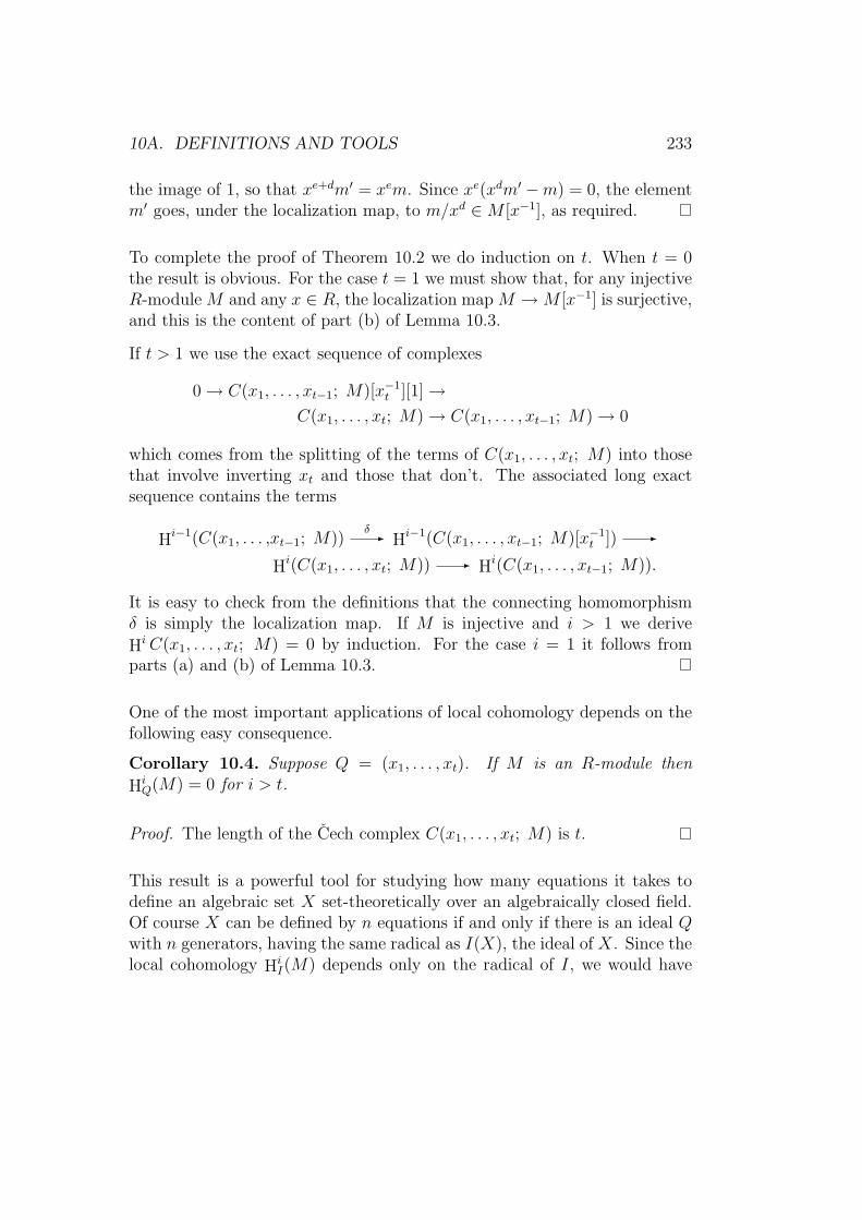
10A. DEFINITIONS AND TOOLS 233
the image of 1, so that xe+dm′ = xem. Since xe(xdm′ −m) = 0, the elementm′ goes, under the localization map, to m/xd ∈M [x−1], as required.
To complete the proof of Theorem 10.2 we do induction on t. When t = 0the result is obvious. For the case t = 1 we must show that, for any injectiveR-module M and any x ∈ R, the localization map M →M [x−1] is surjective,and this is the content of part (b) of Lemma 10.3.
If t > 1 we use the exact sequence of complexes
0 → C(x1, . . . , xt−1; M)[x−1t ][1] →
C(x1, . . . , xt; M) → C(x1, . . . , xt−1; M) → 0
which comes from the splitting of the terms of C(x1, . . . , xt; M) into thosethat involve inverting xt and those that don’t. The associated long exactsequence contains the terms
Hi−1(C(x1, . . . ,xt−1; M))
δ- Hi−1(C(x1, . . . , xt−1; M)[x−1
t ]) -
Hi(C(x1, . . . , xt; M)) - H
i(C(x1, . . . , xt−1; M)).
It is easy to check from the definitions that the connecting homomorphismδ is simply the localization map. If M is injective and i > 1 we derive
HiC(x1, . . . , xt; M) = 0 by induction. For the case i = 1 it follows fromparts (a) and (b) of Lemma 10.3.
One of the most important applications of local cohomology depends on thefollowing easy consequence.
Corollary 10.4. Suppose Q = (x1, . . . , xt). If M is an R-module then
HiQ(M) = 0 for i > t.
Proof. The length of the Cech complex C(x1, . . . , xt; M) is t.
This result is a powerful tool for studying how many equations it takes todefine an algebraic set X set-theoretically over an algebraically closed field.Of course X can be defined by n equations if and only if there is an ideal Qwith n generators, having the same radical as I(X), the ideal of X. Since thelocal cohomology Hi
I(M) depends only on the radical of I, we would have

234CHAPTER 10. APPENDIX A: INTRODUCTION TO LOCAL COHOMOLOGY
HiI(X)(M) = Hi
Q(M) = 0 for all i > n and all modules M . See [Schmittand Vogel 1979] and [Stuckrad and Vogel 1982] for some examples where thistechnique is used, and [Lyubeznik 2002] for a recent survey including manypointers to the literature.
By far the most famous open question of this type is whether each irreduciblecurve in P3
K can be defined set-theoretically by just two equations; it is noteven known whether this is the case for the smooth rational quartic curve Xin P3
K defined as the image of the map
P1K 3 (s, t) → (s4, s3t, st3, t4) ∈ P3
K .
For this curve it is known that HiI(X)(M) = 0 for all i > 2 and all modules
M (see [Hartshorne 1970, Chapter 3]), so the local cohomology test is notuseful here. To add to the fun, it is known that if we replace K by a fieldof characteristic p > 0 then this curve is set-theoretically the complete in-tersection of two surfaces ([Hartshorne 1979]). See [Lyubeznik 1989] for anexcellent review of this whole area.
Change of Rings
Suppose ϕ : R→ R′ is a homomorphism of rings, Q is an ideal of R, and Mis an R′-module. Using the map ϕ we can also regard M as an R-module. Ingeneral, the relation between ExtiR(R/Qd,M) and ExtiR′(R
′/Q′d,M), whereQ′ = QR′, is mysterious (there is a change of rings spectral sequence thathelps a little). For some reason taking the limit, and passing to local coho-mology, fixes this.
Corollary 10.5. Suppose that ϕ : R→ R′ is a homomorphism of Noetherianrings. With notation as above, there is a canonical isomorphism H i
Q(M) ∼=H iQR′(M).
Proof. If x ∈ R is any element, then the localization M [x−1] is the samewhether we think of M as an R-module or an R′-module: it is the setof ordered pairs (m,xd) modulo the equivalence relation (m,xd) (m′, xe) ifxf (xem − xdm′) = 0 for some f . Thus the Cech complex C(x1, . . . , xt; M)is the same whether we regard M as an R-module or an R′-module, and weare done by Theorem 10.2.

10A. DEFINITIONS AND TOOLS 235
Corollary 10.5 fails in the non-Noetherian case even when R = K[t] andI = t; see Exercise 10.9.
Local Duality
Because it comes up so often in applications, we mention a convenient wayto compute local cohomology with respect to the maximal ideal of a homoge-neous polynomial ring. The same method works more generally over regularlocal rings, and, with some care, over arbitrary rings.
Theorem 10.6. Let S = K[x0, . . . , xr] be the polynomial ring, and let m =(x0, . . . , xr) be the homogeneous maximal ideal. If M is a finitely generatedgraded S-module then Hi
m(M) is (as S-module) the graded K-vectorspace dualof Extr+1−i(M,S(−r − 1)).
For a proof see [Brodmann and Sharp 1998, ****].
An Example
A simple example may serve to make all these computations clearer.
Let S = K[x, y], m = (x, y), and consider the S-moduleR = K[x, y]/(x2, xy).We will compute the local cohomology Hi
m(R) (which is the same, by Theo-rem 10.5, is the same as the local cohomology of R as a module over itself)in two ways:
From the Cech complex: The Cech complex of R is by defition
0 - R
(11
)- R[x−1]⊕R[y−1]
(1,−1)- R[(xy)−1] - 0.
However, R is annihilated by x2, and thus also by (xy)2. Thus the Cechcomplex takes the simpler form
0 → R(1)
- R[y−1] - 0,
where the map denoted (1) is the canonical map to the localization.

236CHAPTER 10. APPENDIX A: INTRODUCTION TO LOCAL COHOMOLOGY
The kernel of this map is the 0-th homology of the Cech complex, and thus byTheorem 10.2 it is H0
m(R). As the kernel of the localization map R→ R[y−1]it is the set of elements of R annihilated by a power of y, which is the 1-dimensional vector space
H0m(R) = (x2, xy) : y∞/(x2, xy) = (x)/(x2, xy) = K · x.
Since the localization map kills x, we see that R[y−1] = S/(x)[y−1], and theimage of R in R[y−1] is the same as the image of S/(x) in S/(x)[y−1]. Thusthe first homology of the Cech complex, which is equal by Theorem 10.2 tothe first local cohomology of R, is
H1m(R) = S/(x)[y−1]/(S/(y)) = K · y−1 ⊕K · y−2 ⊕ · · · = K(1)⊕K(2)⊕ · · · .
From local duality: Because (x2, xy) is generated by just two elements itis easy to write down a free resolution of S/(x2, xy):
0 - S(−3)
(y−x
)- S2(−2)
(x2 xy )- S - R - 0
The modules ExtiS(R,S) = ExtS(R,S) are the homology of the dual complex,twisted by −2, which is
0 S(1) (y −x )
S2
(x2
xy
)S(−2) 0.
It is thus immediate that Ext0S(R,S(−2)) = 0. We also see at once that
Ext2S(R, S(−2)) = (S(3)/(x, y))(−2) = K(1), the dual of K(−1) = H0
m(R)as claimed by Theorem 10.6.
To analyze Ext1S(R,S(−2)) = 0 we note that the actual kernel of the map
S(1) (y −x )
S2
is
S2
(xy
)S(−1),
so the desired homology is
Ext1S(R, S(−2)) = S ·(x, y)/S ·(x2, xy) = S/(x)(−1) = K(−1)⊕K(−2)⊕· · · ,
which is indeed the dual of the local cohomology module H1m(R) as computed
above.

10B. LOCAL COHOMOLOGY AND SHEAF COHOMOLOGY 237
10B Local cohomology and sheaf cohomology
If M is any module over a Noetherian ring R and Q = (x1, . . . , xt) ⊂ R isan ideal, then M gives rise by restriction to a sheaf FM on the affine schemeSpecR \V (Q) whose i-th Zariski cohomology Hi(FM) may be defined as thei-th cohomology of the Cech complex
Cech(x1, . . . , xt; M) :
0 - ⊕t1 M [x−1
i ]d- · · · ⊕#J=sM [x−1
J ]d- · · ·M [x−1
1,...,t]- 0
whose differential is defined as in Theorem 10.2. The reader who has not yetstudied schemes and their cohomology should think of Hi(FM) as a functorof M without worrying about the nature of FM . The definition is actuallyindependent of the choice of generators x1, . . . , xt for Q; one can show that
H0(FM) = limd Hom(Qd,M), sometimes called the ideal transform of M withrespect to Q (see Exercise 10.3). Further, Hi(M) is the i-th right derivedfunctor of the ideal transform functor—this follows just as in the proof ofTheorem 10.2. When R and M are standard graded algebras, we will seebelow that Hi(FM) is a sum of the usual i-th cohomology modules of thesheaves M(d) on the projective variety ProjR.
The local cohomology is related to Zariski cohomology in a simple way:
Proposition 10.7. If Q = (x1, . . . , xt) then:(a) There is an exact sequence of R-modules
0 → H0Q(M) →M → H0(FM) → H1
Q(M) → 0.
(b) For every i ≥ 2
H iQ(M) =
⊕d
H i−1(FM).
Proof. Note that Cech(x1, . . . , xt; M) is the subcomplex of the complexC(x1, . . . , xt; M) obtained by dropping the first term, M ; so we get anexact sequence of complexes
0 → Cech(x1, . . . , xt; M)[−1] → C(x1, . . . , xt; M) →M → 0

238CHAPTER 10. APPENDIX A: INTRODUCTION TO LOCAL COHOMOLOGY
where M is regarded as a complex with just one term, in degree 0. Sincethis one-term complex has no higher cohomology, the long exact sequence incohomology coming from this short exact sequence of complexes gives exactlystatements (a) and (b).
Henceforward we will restrict our attention to the case where R is the poly-onomial ring S = K[x0, . . . , xr], the ideal Q is the homogeneous maximalideal Q = (x0, . . . , xr), and the module M is finitely generated and graded.It follows that all the cohomology is graded too. Following our usual con-vention we will write Hi
Q(M)d for the d-th graded component of HiQ(M), and
similarly for the Zariski cohomology of FM .
Another way to express H0Q(M) in our special case is to say that it is the
largest submodule of M having finite length. To see this, note that anysubmodule N ⊂M of finite length is (by Nakayama’s lemma) annihilated bya power of Q. Conversely, the submodule H0
Q(M) is finitely generated, andeach of its generators is annihilated by a power of Q. Thus it is a finitelygenerated module over the ring of finite length S/Qd for sufficiently large d.
In this setting the Zariski cohomology has another interpretation: Any gradedS-module M gives rise to a quasicoherent sheaf M on the projective spacePr (for the definition and properties of this construction see for example[Hartshorne 1977, II.5].) The Cech complex for M is the degree 0 part ofthe complex Cech(x0, . . . , xr; M). In particular, the i-th (Zariski) cohomol-ogy of the sheaf M is the degree 0 part of the cohomology of FM , that is
Hi(M) = Hi(FM)0. If we shift the grading of M by d to get M(d), then M(d)is the sheaf on Pr associated to M(d), so in general Hi(M(d)) = Hi(FM)d.Thus Theorem 10.7 takes on the following form:
Corollary 10.8. Let M be a graded S-module, and let M be the correspond-ing quasicoherent sheaf on Pr.(a) There is an exact sequence of graded S-modules
0 → H0Q(M) →M →
⊕d
H0(M(d)) → H1Q(M) → 0.
(b) For every i ≥ 2H iQ(M) =
⊕d
H i−1(M(d)).

10B. LOCAL COHOMOLOGY AND SHEAF COHOMOLOGY 239
As a first example, Proposition 10.8 lets us compute the local cohomology ofthe polynomial ring as a module over itself in terms of the well-known sheafcohomology of line bundles on Pr.
Corollary 10.9. If S = K[x0, . . . , xr] with r ≥ 1 then
H iQ(S)d =
0 if i ≤ rHomK(S−r−1−d,K) if i = r + 1.
Proof. This is an immediate consequence of Proposition 10.8, given the co-homology of OPr(d) = S(d) (see [Hartshorne 1977, III.3.1]).
It is also easy to calculate the local cohomology of a module of finite length:it has (almost) none!
Corollary 10.10. If M is a graded S-module of finite length, then H0Q(M) =
M , while H iQ(M) = 0 for i > 0.
Note the contrast with the case of ExtiS(S/Qj,M); for example when M
is the module K, of length 1: here the value is nonzero for all j and all0 ≤ i ≤ r. The Corollary says that in the limit everything goes to zeroexcept when i = 0!
Proof. The first assertion is the definition of H0Q(M) = 0 in this case. Since
a power of each xi annihilates M , we have M [x−1i ] = 0 for each i, whence the
sheaf M is zero. Thus the second assertion follows from Proposition 10.8.
The final result of this section explains the gap between the Hilbert functionand the Hilbert polynomial:
Corollary 10.11. Let M be a finitely generated graded S-module. For everyd ∈ Z
PM(d) = HM(d)−∑i≥0
(−1)i dimK HiQ(M)d.
Proof. The Euler characterisitic of the sheaf M(d) is by definition
χ(M(d)) =∑i≥0
(−1)i dimK Hi M(d).

240CHAPTER 10. APPENDIX A: INTRODUCTION TO LOCAL COHOMOLOGY
We first claim that PM(d) = χ(M(d)) for every d. Indeed, by Serre’s Vanish-ing Theorem (see [Hartshorne 1977, Chapter 3]) Hi(M(d)) vanishes for i > 0when d 0 so χ(M(d)) = dimK H0(M(d)) = Md for large d. Thus for theclaim it suffices to show that χ(M(d)) is a polynomial function of d. This isdone by induction: if x is a general linear form on Pr then from the exactsequence
0 → M(−1)x- M - M/xM → 0
we derive a long exact sequence in cohomology which (since it has only finitelymany terms) establishes the recursion formula
χ(M(d))− χ(M(d− 1)) = χ(M/xM(d)).
Since the support of ˜M/xM equals the hyperplane section of the support of
M , we see by induction on the dimension of the suport of M that χ( ˜M/xM(d))is a polynomial, and thus χ(M(d)) is also.
By Corollary 10.8 we have
χ(M(d)) = dimK H0(M(d))−
∑i≥1
(−1)i dimK Hi(M(d))
= dimK Md − dimK H0Q(M)d + dimK H
1Q(M)d −
∑i≥2
(−1)i dimK HiQ(M)d
as required.
10C Vanishing and nonvanishing theorems
In this section we maintain the hypothesis that S = K[x0, . . . , xr], the idealQ is the homogeneous maximal ideal Q = (x0, . . . , xr), and the module M isfinitely generated and graded.
The converse of Corollary 10.10 is also true; it is a special case of the di-mension assertion in the following result. The proofs of the next two resultsrequire slightly more sophisticated commutative algebra than what has gonebefore, and we will not use them in the sequel. We include them to give aflavor of the usefulness of local cohomology.
Proposition 10.12. Let M be a finitely generated graded S-module.

10C. VANISHING AND NONVANISHING THEOREMS 241
1. If i < depthM or i > dimM then H iQ(M) = 0.
2. If i = depthM or i = dimM then H iQ(M) 6= 0.
In between the depth and the dimension almost anything can happen; see[Evans and Griffith 1979].
Proof. Usng the fact that Exti(S/Qn,M) = 0 for i < depth(Q,M) (see[Eisenbud 1995, Proposition 18.4]) we see that H i
Q(M) = 0 in this range.From Proposition 10.8 and Grothendieck’s Theorem (see [Hartshorne 1977,Theorem III.2.7]) that sheaf cohomology vanishes in degrees above the di-mension of the support of the sheaf, we see that H i
Q(M) = 0 for i > dimM .This proves part 1.
For the nonvanishing we use the fact that the local cohomology is a derivedfunctor and thus we get a long exact sequence in local cohomology fromany short exact sequence of modules. To prove that H i
Q(M) 6= 0 wheni = depthM we do induction on depthM . If the depth is zero then everyelement of positive degree is a zero divisor on M . The set of zero divisorson M is the union of the associated primes of M , so this says that Q iscontained in the union. It follows from the “prime avoidance lemma” thatQ is an associated prime of M , that is, M contains a copy of S/Q, a moduleof finite length, and thus H0
Q(M) 6= 0.
If, on the other hand, the depth is positive, then we can choose a homoge-neous nonzerodivisor f on M . We have depthM/fM = depthM − 1. If thedegree of f is d, we have a short exact sequence
0 →M →M(d) →M/fM(d) → 0,
and by inductionHdepthM−1Q M/fM(d) 6= 0. On the other handHdepthM−1
Q M(d) =0 by part 1, so the resulting long exact sequence
· · · → HdepthM−1Q M(d) → HdepthM−1
Q M/fM(d) → HdepthMQ M → · · ·
shows that HdepthMQ M 6= 0.
To prove that HdimMQ M 6= 0 we proceed by induction on dimM . Let
M = M/H0Q(M). For i > 0 we have H i
Q(H0QM) = 0 by Corollary 10.10, so

242CHAPTER 10. APPENDIX A: INTRODUCTION TO LOCAL COHOMOLOGY
H iQ(M) = H i
Q(M/(H0QM)). Further, H0
Q(M/(H0QM)) = 0. Since dimM =
dimM/(H0QM), we may thus suppose H0
QM = 0.
It follows as above that Q is not an associated prime of M , and we maychoose a nonzerodivisor f on M as before. As dimM/fM = dimM − 1 wemay replace the depth in the argument above by the dimension, and concludethat HdimM
Q M 6= 0 as required.
Finally, we use the theory developed to study the map M → ⊕dH0(M(d)).
Recall that the normalization of a domain is its integral closure in its field offractions, and that when we speak of a variety we assume it to be irreducible.
Corollary 10.13. Let M be a finitely generated graded S-module. The nat-ural map M → ⊕dH
0(M(d)) is an isomorphism if and only if depthM ≥ 2.If M = SX is the homogeneous coordinate ring of a normal projective varietyX of dimension at least 1, then ⊕dH
0(OX(d)) is the normalization of SX .
Proof. We have already seen that depthM ≥ 2 if and only if H iQM = 0
for i = 0, 1 and the first assertion now follows from the first assertion ofProposition 10.8.
For the second assertion, set R = ⊕dH0(OX(d)). Thus R is a domain con-
taining SX .
To show that R is integral over SX we use the finiteness of cohomology andSerre’s vanishing theorem: Suppose 0 6= f ∈ H0OX(d). As X is a variety ofdimension ≥ 1 we must have d > 0.
For the case d = 0 we note that R0 = H0OX is a finite dimensional K-vectorspace. It follows that f satisfies an algebraic equation with coefficients in K,so it is integral over K and thus necessarily integral over (SX)0.
To take care of the case d > 0, we may assume r ≥ 2 (otherwise X = P1 andSX = K[x0, x1] = R to begin with). We use the sequence
0 → IX → OPr → OX → 0.
Since r ≥ 2 we have H1OPr(d) = 0 for all d, so the long exact sequence gives⊕d
H1IX(d) = coker(⊕d
H0OPr(d) →⊕d
H0OX(d)) = cokerSX → R = H1QSX

10C. VANISHING AND NONVANISHING THEOREMS 243
by Proposition 10.8 (we have used the fact that SX is the image of⊕
dH0OPr(d) =
S in⊕
dH0OX(d)) = R.) By Serre’s vanishing theorem, (H1
QSX)e = 0 andRe = (SX)e for e >> 0, whence a large power of f must be in SX , provingthat f is integral in this case too. Notice that our argument proves thatelements of non-negative degree in R are integral over SX whether or not thedimension of X is at least 1 and whether or not X is irreducible.
It now suffices to show that R is normal. For this we use Serre’s criterion: Adomain R is normal if RP is regular for every associated prime P of a principalideal in R (see [Eisenbud 1995, Theorem 11.2]). In the graded case, we mayasssume that the principal ideal is generated by a homogeneous element (Thisfollows as in the reference given, once we remark that the integral closureof R would have to be generated by homogeneous elements.) Suppose thatP ⊂ R is associated to a principal ideal of R, and let P ′ = P ∩ SX . SinceX is a normal variety, the localization of SX at any homogeneous prime P ′
other than Q is the local ring of X along a subvariety, with a variable andits inverse adjoined. Since X is normal, so is (SX)P ′ , and thus (SX)P ′ = RP ,and P cannot be associated to a principal ideal unless RP is regular.
There remains the case where P ′ = Q, the maximal homogeneous ideal.Because R is integral over SX , and R+ ∩ S = Q, while P ⊂ R+, we musthave P = R+ by “incomparability” (see [Eisenbud 1995, Corollary 4.18]).We will show that this case cannot occur by showing that depth(R+, R) ≥ 2.
To this end, choose any homogeneous element 0 6= f ∈ R of positive degreed, say. Since R is a domain we have a short exact sequence
0 → R(−d) f- R - R/fR→ 0.
Sheafifying and taking homology we get a long exact sequence containing theterms
0 → R(−d) f- R -⊕d
H0(R/fR)(d) → · · · ,
where we have used the first statement of Corollary 10.13 to identify⊕
dH0(R)(d)
with R.
Again by the first statement of Corollary 10.13 we haveH0Q(⊕
dH0(R/fR)(d)) =
0, whence H0Q(R/fR) = 0, so Q and a fortiori P contains a nonzerodivisor
on R/fR, and P is not associated to fR. Since all maximal regular se-

244CHAPTER 10. APPENDIX A: INTRODUCTION TO LOCAL COHOMOLOGY
quences have the same length, P is not associated to any principal ideal ofR generated by a nonzerodivisor.
In the subjects we deal with elsewhere in this book it is really a matter oftaste whether one uses local cohomology or sticks with the language of coher-ent sheaf cohomology, passing to the cohomology of various syzygy modulesto replace the “missing” groups H0
Q and H1Q. But using local cohomology
makes the statements much simpler and more uniform, so we have given itpreference.
10D Exercises
1. Cofinality: Let R ⊃ J1 ⊃ J2 ⊃ . . . and R ⊃ K1 ⊃ K2 ⊃ . . . besequences of ideals in a ring R, and suppose that there exist functionsm(i) and n(i) such that Ji ⊃ Km(i) and Ki ⊃ Jn(i) for all i. Show thatfor any R-module M we have
limi
ExtpR(S/Ji,M) = limi
ExtpR(S/Ki,M).
2. Use Exercise 10.1 and the Artin Rees Theorem to show that if R is aNoetherian ring containing ideals Q1 and Q2, and M is an R-module,then there is a long exact sequence
· · · →HiQ1+Q2
(M) → HiQ1
(M)⊕ HiQ2
(M) → HiQ1∩Q2
(M) →Hi+1Q1+Q2
(M) → · · ·
3. Let R be a Noetherian ring, and Q an ideal of R. Let F be a coher-ent sheaf on SpecR \ V (Q). Prove that H0(FM) = limHom(Qd,M)by defining maps in both directions mi/x
di 7→ [f : xei 7→ xe−di mi]
restricted to Q(r+1)e ⊂ (xe0, . . . , xer) for big e; and [f : Qd → M ] 7→
f(xdi )/xdi .
4. Prove that for any R-module M over any Noetherian ring we have
limd
Hom((xd),M) = M [x−1].

10D. EXERCISES 245
5. Show that the complex C(x1, . . . , xt; M) is the direct limit of theKoszul complexes. Use this to give another proof of Theorem 10.2in the case where x1, . . . , xt is a regular sequence in R.
6. Compute the local cohomology of the module S in the cases S = K[x0]and S = K not treated in Corollary 10.9
7. Use Corollary 10.12 to prove Grothendieck’s Vanishing Theorem: IfF is a coherent sheaf F on Pr whose support has dimenion n then
Hi(F) = 0 for i > n. (Hint: choose a system of parameters for Sconsisting of elements in annM and dimM further elements, and useTheorem 10.2.
8. Let R be the ring R = k[x, y1, y2, . . .]/(xy1, x2y2, . . .). Note that R is
non-Noetherian: for example the sequence of ideals ann(xn) increasesforever. Show that the formula in Exercise 10.4 fails over this ring forM = R.
9. Let R be any ring containing an element x such that the sequenceof ideals ann(xn) increases forever. If an R-module M contains R,show that the map M →M [x−1] cannot be surjective; that is the firsthomology of the Cech complex
0 →M →M [x−1] → 0
is nonzero. In particular, this is true for the injective envelope of R inthe category of R-modules. Conclude that the cohomology of this Cechcomplex ofM does not compute the derived functors of the functor H0
Rx,and in particular that Corollary 10.5 fails for the map Z[t] → R witht 7→ x.

246CHAPTER 10. APPENDIX A: INTRODUCTION TO LOCAL COHOMOLOGY

Chapter 11
Appendix B: A Jog ThroughCommutative Algebra
Revised 9/11/03
((Get rid of “Chapter 11” — this is appendix B))
My goal in this appendix is to lead the reader on a brisk jog through thegarden of commutative algebra. There won’t be time to smell many flowers,but I hope to impart an overview of the landscape, at least of that part ofthe subject used in this book.
Each section is focused on a single topic. It begins with some motivationand the principle definitions, and then lists some central results, often withillustrations of their use. Finally, there are some further, perhaps more subtle,examples. There are practially no proofs; these can be found, for example,in my book [Eisenbud 1995].
I assume that the reader is familar with
• Rings, ideals, and modules, and occasionally some homological notions,such as Hom and ⊗, Ext and Tor.
• Prime ideals and the localizations of a ring
• The correspondence between affine rings and algebraic sets
247

248CHAPTER 11. APPENDIX B: A JOG THROUGH COMMUTATIVE ALGEBRA
There are a few references to sheaves and schemes, but these can be harm-lessly skipped.
The topics to be treated are:
1. Associated primes
2. Depth
3. Projective dimension and regular local rings
4. Normalization (resolution of singularities for curves)
5. The Cohen-Macaulay property
6. The Koszul complex
7. Fitting ideals
8. The Eagon-Northcott complex and scrolls
Throughout, K denotes a field and R denotes a commutative Noetherianring. The reader should think primarily of the cases whereR = K[x1, . . . , xn]/Ifor some ideal I, or where R is the localization of such a ring at a primeideal. Perhaps the most interesting case of all is when R is a homogeneous(or standard graded) algebra, by which we mean a graded ring of the formR = K[x0, . . . , xr]/I, where all the xi have degree 1, and I is a homogeneousideal (that is, a polynomial f is in I iff each homogeneous component of fis in I).
There is a fundamental similarity between the local and the homogeneouscases. Many results for local rings depend on Nakayama’s Lemma, whichstates (in one version) that ifM is a finitely generated module over a local ringR with maximal ideal m and g1, . . . , gn ∈ M are elements whose images inM/mM generate M/mM , then g1, . . . , gn generate M . A closely analogousresult is true in the homogeneous situation: if M is a finitely generatedgraded module over a homogeneous ring R with maximal homogeneous idealm =
∑d>0Rd, and if g1, . . . , gn ∈M are homogeneous elements whose images
in M/mM generate M/mM , then g1, . . . , gn generate M . These results canbe unified: following Goto and Watanabe [* ref: Generalized Local Rings I,

11A. ASSOCIATED PRIMES AND PRIMARY DECOMPOSITION. 249
II] one can define a generalized local ring to be a graded ring R = R0⊕R1⊕. . .such that R0 is a local ring. If m is the maximal homogeneous ideal, thatis, the sum of the maximal ideal of R0 and the ideal of elements of strictlypositive degree, then Nakayama’s Lemma holds for R and a finitely generatedgraded R-module M just as before.
Similar homogeneous versions are possible for many results involving localrings. Both the local and homogeneous cases are important, but rather thanspelling out two versions of every theorem, or passing to the generality ofgeneralized local rings, we usually give only the local version.
11A Associated Primes and primary decom-
position.
11A.1 Motivation and Definitions
Any integer admits a unique decomposition as a product of primes and a unit.Attempts to generalize this result to rings of integers in number fields werethe number-theoretic origin of commutative algebra. With the work of Laskerand Macaulay around 1900 the theorems took something like their final formfor the case of polynomial rings, the theory of primary decomposition. It wasEmmy Noether’s great contribution to see that they followed relatively easilyfrom just the ascending chain condition on ideals. (Indeed, modern workhas shown that most of the important statements of the theory fail in thenon-Noetherian case). Though the full strength of primary decomposition israrely used, the concepts involved are fundamental, and some of the simplestcases are pervasive.
The first step is to recast the unique factorization of an integer n ∈ Z into aunit and a product of powers of distinct primes, say
n = ±∏i
paii ,
as a result about intersections of ideals, namely
(n) =⋂i
(paii ).

250CHAPTER 11. APPENDIX B: A JOG THROUGH COMMUTATIVE ALGEBRA
In the general case we will again express an ideal as an intersection of ideals,called primary ideals, each connected to a particular prime ideal.
Recall that a proper ideal I ⊂ R (that is, an ideal not equal to R) is prime ifxy ∈ I and x /∈ I implies y ∈ I. If M is a module then a prime ideal P is saidto be associated to M if P = annm, the annihilator of some m ∈ M . Wewrite AssM for the set of associated primes of M . The module M is calledP -primary if P is the only associated prime of M . The most important caseoccurs when I ⊂ R is an ideal and M = R/I; then it is traditional to saythat P is associated to I when P is associated to R/I, and to write Ass I inplace of AssR/I. We also say that I is P -primary if R/I is P -primary. (Theconfusion this could cause is rarely a problem: usually the associated primesof I as a module are not very interesting.) The reader should check that theassociated primes of an ideal (n) ⊂ Z are those (p) generated by the primedivisors p of n. In particular, the (p)-primary ideals in Z are exactly thoseof the form (pa).
For any ideal I we say that a prime P is minimal over I if P is is minimalamong primes containing I. An important set of primes connected with amodule M is the set MinM of primes minimal over the annihilator I =annM . These are called the minimal primes of M . Again we abuse theterminology, and when I is an ideal we define the minimal primes of I to bethe minimal primes over I, or equivalently the minimal primes of the moduleR/I. We shall see below that all minimal primes of M are associated to M .The associated primes of M that are not minimal are called embedded primesof M .
11A.2 Results
Theorem 11.1. Let M be a nonzero finitely generated R-module.
1. MinM ⊂ AssM , and both are nonempty finite sets.
2. The set of elements of R that are zerodivisors on M is the union of theassociated primes of M .
If M is a graded module over a homogeneous ring R, then all the associatedprimes of M are homogeneous.

11A. ASSOCIATED PRIMES AND PRIMARY DECOMPOSITION. 251
Among the most useful Corollaries is the following.
Corollary 11.2. If I is an ideal of R and M is a finitely generated modulesuch that every element of I annihilates some nonzero element of M , thenthere is a single nonzero element of M annihilated by all of I. In particular,any ideal of R that consists of zerodivisors is annihilated by a single element.
The proof is immediate from Theorem 11.1 given the “prime avoidancelemma”.
Lemma 11.3. If an ideal I is contained in a finite union of prime ideals,then it is contained in one of them.
It is easy to see that an element f ∈ R is contained in an ideal I iff the imageof f in the localization RP is contained in IP for all prime ideals, or even justfor all maximal ideals P of R. Using Theorem 11.1 one can pinpoint the setof localizations it is necessary to test, and see that this set is finite.
Corollary 11.4. If f ∈M , then f = 0 iff the image of f is zero in MP foreach associated prime P of M . It even suffices that this condition is satisfiedat each maximal associated prime of M .
One reason for looking at associated primes for modules, and not only forideals, is the following useful result, which is a component of the proof ofTheorem 11.1.
Theorem 11.5. Let 0 → M ′ → M → M ′′ → 0 be a short exact sequence offinitely generated R-modules. We have
Ass(M ′) ⊂ Ass(M) ⊂ Ass(M ′) ∪ Ass(M ′′).
If M = M ′ ⊕M ′′ then the second inclusion becomes an equality.
Here is the primary decomposition result itself.
Theorem 11.6. If I is an ideal of R then Ass(R/I) is the unique minimalset of prime ideals S such that we can write I = ∩P∈SQP , where QP is aP -primary ideal (there is a similar result for modules).
In this decomposition the ideals QP with P ∈ Min I are called minimalcomponents and are unique. The others are called embedded componentsand are generally non-unique.

252CHAPTER 11. APPENDIX B: A JOG THROUGH COMMUTATIVE ALGEBRA
11A.3 Examples
1. Primary decomposition translates easily into geometry by means ofHilbert’s Nullstellensatz [Eisenbud 1995, Theorem 1.6]. Here is a sam-ple that contains a fundamental finiteness principle. Recall that theradical of an ideal I, written
√I, is the ideal
√I = f ∈ R | fm ∈ I for some m.
We say that I is radical if I =√I. The primary decomposition of a
radical ideal has the form√I = ∩P∈Min IP.
Any algebraic set X (say in affine n-space AnK over an algebraically
closed field K, or in projective space) can be written uniquely as a finiteunion X = ∪iXi of irreducible sets. The ideal I = I(X) of functionsvanishing on X is the intersection of the prime ideals Pi = I(Xi). Theexpression I = ∩iPi is the primary decomposition of I.
2. For any ring R we write K(R) for the result of localizing R by invertingall the nonzerodivisors of R. By Theorem 11.1, this is the localizationof R at the complement of the union of the associated primes of R, andthus it is a ring with finitely many maximal ideals. Of course if R isa domain then K(R) is simply its quotient field. The most useful casebeyond is when R is reduced. ThenK(R) = K(R/P1)×· · ·×K(R/Pm),the product of the quotient fields of R modulo its finitely many minimalprimes.
3. Let R = K[x, y] and let I = (x2, xy). The associated primes of I are (x)and (x, y), and a primary decomposition of I is I = (x) ∩ (x, y)2. Thismight be read geometrically as saying: for a function f(x, y) to lie in I,the function must vanish on the line x = 0 in K2 and vanish to order2 at the point (0, 0). In this example, the (x, y)-primary component(x, y)2 is not unique: we also have I = (x)∩ (x2, y). The correspondinggeometric statement is that a function f lies in I if and only if f vanisheson the line x = 0 in K2 and (∂f/∂x)(0, 0) = 0.
4. If P is a prime ideal, the powers of P may fail to be P -primary! Ingeneral, the P -primary component of Pm is called the m-th symbolic
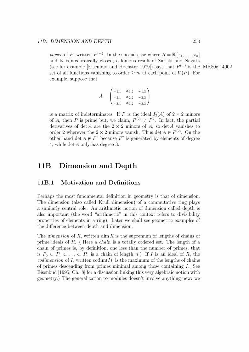
11B. DIMENSION AND DEPTH 253
power of P , written P (m). In the special case where R = K[x1, . . . , xn]and K is algebraically closed, a famous result of Zariski and Nagata(see for example [Eisenbud and Hochster 1979]) says that P (m) is the MR80g:14002set of all functions vanishing to order ≥ m at each point of V (P ). Forexample, suppose that
A =
x1,1 x1,2 x1,3
x2,1 x2,2 x2,3
x3,1 x3,2 x3,3
is a matrix of indeterminates. If P is the ideal I2(A) of 2 × 2 minorsof A, then P is prime but, we claim, P (2) 6= P 2. In fact, the partialderivatives of detA are the 2 × 2 minors of A, so detA vanishes toorder 2 wherever the 2 × 2 minors vanish. Thus detA ∈ P (2). On theother hand detA /∈ P 2 because P 2 is generated by elements of degree4, while detA only has degree 3.
11B Dimension and Depth
11B.1 Motivation and Definitions
Perhaps the most fundamental definition in geometry is that of dimension.The dimension (also called Krull dimension) of a commutative ring playsa similarly central role. An arithmetic notion of dimension called depth isalso important (the word “arithmetic” in this context refers to divisibilityproperties of elements in a ring). Later we shall see geometric examples ofthe difference between depth and dimension.
The dimension of R, written dimR is the supremum of lengths of chains ofprime ideals of R. ( Here a chain is a totally ordered set. The length of achain of primes is, by definition, one less than the number of primes; thatis P0 ⊂ P1 ⊂ . . . ⊂ Pn is a chain of length n.) If I is an ideal of R, thecodimension of I, written codim(I), is the maximum of the lengths of chainsof primes descending from primes minimal among those containing I. SeeEisenbud [1995, Ch. 8] for a discussion linking this very algebraic notion withgeometry.) The generalization to modules doesn’t involve anything new: we

254CHAPTER 11. APPENDIX B: A JOG THROUGH COMMUTATIVE ALGEBRA
define the dimension dimM of an R-module M to be the dimension of thering R/ ann(M)
A sequence x = x1, . . . , xn of elements of R is a regular sequence (or R-sequence) if x1, . . . , xn generate a proper ideal of R and if, for each i, theelement xi is a nonzerodivisor modulo (x1, . . . , xi−1). Similarly, if M is an R-module, then x is a regular sequence on M (orM -sequence) if (x1, . . . , xn)M 6=M and, for each i, the element xi is a nonzerodivisor on M/(x1, . . . , xi−1)M .
If I is an ideal of R and M is a finitely generated module such that IM 6= M ,then the depth of I onM , written depth(I,M), is the maximal length of a reg-ular sequence on M contained in I. (If IM = M we set depth(I,M) = ∞.)The most interesting cases are the ones where R is a local or homoge-neous ring and I is the maximal (homogeneous) ideal. In these cases wewrite depth(M) in place of depth(I,M). We define the grade of I to begrade(I) = depth(I, R). (Alas, terminology in this area is quite variable; seefor example [Bruns and Herzog 1998, Section 1.2] for a different system.) Weneed one further notion of dimension, a homological one that will reappear inthe next section. The projective dimension of an R-module is the minimumlength of a projective resolution of M (or ∞ if there is no finite projectiveresolution.)
11B.2 Results
We will suppose for simplicity that R is local with maximal ideal m. Similarresults hold in the homogeneous case. A fundamental geometric observationis that a variety over an algebraically closed field that is defined by oneequation has codimension at most 1. The following is Krull’s justly celebratedgeneralization.
Theorem 11.7. (Principal Ideal Theorem). If I is an ideal that can be gen-erated by n elements in a Noetherian ring R, then grade(I) ≤ codim(I) ≤ n.Moreover, any prime minimal among those containing I has codimension atmost n. If M is a finitely generated R-module, then dimM/IM ≥ dimM−n.
For example, in R = K[x1, . . . , xn] or R = K[x1, . . . , xn](x1,...,xn) or R =K[[x1, . . . , xn]] the sequence x1, . . . , xn is a maximal regular sequence. Itfollows at once from Theorem 11.7 that in each of these cases the ideal

11B. DIMENSION AND DEPTH 255
(x1, . . . , xn) has codimension n, and for the local ringR = K[x1, . . . , xn](x1,...,xn)
or R = K[[x1, . . . , xn]] this gives dimR = n. For the polynomial ring R it-self this argument gives only dimR ≥ n, but in fact it is not hard to showdimR = n in this case as well. This follows from a general result on affinerings.
Theorem 11.8. If R is an integral domain with quotient field K(R), andR is a finitely generated algebra over the field K, then dimR is equal to thetranscendence degree of K(R) over K. Geometrically: the dimension of analgebraic variety is the number of algebraically independent functions on it.
The following is a generalization of Theorem 11.7 in which the ring R isreplaced by an arbitrary module.
Theorem 11.9. If M is a finitely generated R-module and I ⊂ R is an ideal,then
depth(I,M) ≤ codim((I + annM)/(annM)) ≤ dimM.
A module is generally better behaved—more like a free module over a poly-nomial ring—if its depth is close to its dimension. See also Theorem 11.11.)
Theorem 11.10. If R is a local ring and M is a finitely generated R-modulethen
1. All maximal regular sequences on M have the same length; this commonlength is equal to the depth of M . Any permutation of a regular sequenceon M is again a regular sequence on M .
2. depth(M) = 0 iff Ass(M) contains the maximal ideal (see Theorem11.1(2)).
3. For any ideal I, depth(I,M) = infi | ExtiR(R/I,M) 6= 0.
4. If R = K[x0, . . . , xr] with the usual grading, M is a finitely generatedgraded R-module, and m = (x0, . . . , xr), then depth(M) = infi |Hi
m(M) 6= 0.
Parts 3 and 4 of Theorem 11.10 are connected by what is usually called localduality ; see Theorem 10.6.

256CHAPTER 11. APPENDIX B: A JOG THROUGH COMMUTATIVE ALGEBRA
Theorem 11.11. (Auslander-Buchsbaum formula). If R is a local ring andM is a finitely generated R-module such that pd(M) (the projective dimensionof M) is finite, then depth(M) = depth(R)− pd(M).
The following results follow from Theorem 11.11 by localization.
Corollary 11.12. Suppose that M is a finitely generated module over a localring R.
1. If M has an associated prime of codimension n, then pd(M) ≥ n.
2. If M has finite projective dimension, then pd(M) ≤ depthR ≤ dimR.If pd(M) = 0 then M is free.
3. If pd(M) = dimR then R is Cohen-Macaulay and the maximal ideal isassociated to M .
Another homological characterization of depth, this time in terms of theKoszul complex, is given in Section 11G.
11B.3 Examples
1. Theorem 11.10 really requires the “local” hypothesis (or, of course, theanalogous “graded” hypothesis). For example, in K[x] × K[y, z] thesequences (1, y), (0, z) and (x, 1) are both maximal regular sequences.Similarly, in R = K[x, y, z] the seqence x(1− x), 1− x(1− y), xz is a aregular sequence but its permutation x(1−x), xz, 1−x(1−y) is not. Theideas behind these examples are related: R/(x(1−x)) = K[y, z]×K[y, z]by the Chinese Remainder Theorem.

11C. PROJECTIVE DIMENSION 257
11C Projective dimension and regular local
rings
11C.1 Motivation and Definitions
After dimension, the next most fundamental geometric ideas may be those ofsmooth manifolds and tangent spaces. The analogues in commutative algebraare regular rings and Zariski tangent spaces, introduced by Krull [Krull 1937]and Zarisk [Zariski 1947]. Since the work of Auslander, Buchsbaum, andSerre in the 1950s this theory has been connected with the idea of projectivedimension.
Let R be a local ring with maximal ideal m. The Zariski cotangent space ofR is m/m2, regarded as a vector space over R/m; the Zariski tangent spaceis the dual, HomR/m(m/m2, R/m). The ring R is called regular if its Krulldimension, dim(R), is equal to the dimension of the Zariski tangent space(as a vector space); otherwise, R is singular. If R is a Noetherian ring thatis not local, we say that R is regular if each localization at a maximal idealis regular.
For example, the n-dimensional power series ring
K[[x1, . . . , xn]]
is regular because the maximal ideal m = (x1, . . . , xn) satisfies m/m2 =⊕n
1Kxi. The same goes for the localization of the polynomial ring K[x1, . . . , xn](x1, . . . , xn).Indeed any localization of one of these rings is also regular though this isharder to prove; see Corollary 11.15.
11C.2 Results
Here is a first taste of the consequences of regularity.
Theorem 11.13. Any regular local ring is a domain. A local ring is regulariff its maximal ideal is generated by a regular sequence.
The following result initiated the whole homological study of rings.

258CHAPTER 11. APPENDIX B: A JOG THROUGH COMMUTATIVE ALGEBRA
Theorem 11.14. (Auslander-Buchsbaum-Serre). A local ring R is regulariff the residue field of R has finite projective dimension iff every R-modulehas finite projective dimension.
The abstract-looking characterization of regularity in Theorem 11.14 alloweda proof of two properties that had been known only in the “geometric” case(R a localization of a finitely generated algebra over a field). These werethe first triumphs of representation theory in commutative algebra. Recallthat a domain R is called factorial if every element of r can be factored intoa product of prime elements, uniquely up to units and permutation of thefactors.
Theorem 11.15. Any localization of a regular local ring is regular. Everyregular local ring is factorial (that is, has unique factorization of elementsinto prime elements.)
The first of these statements is, in the geometric case, a weak version of thestatement that the singular locus is a closed subset. The second plays animportant role in the theory of divisors.
11C.3 Examples
1. The rings
K[x1, . . . , xn], K[x1, . . . , xn, x−11 , . . . , x−1
n ], and K[[x1, . . . , xn]]
are regular, and the same is true if K is replaced by the ring of integersZ.
2. A regular local ring R of dimension 1 is called a discrete valuationring. By definition, the maximal ideal of R must be principal; let π bea generator. By Theorem 11.13 R is a domain. Conversely, any onedimensional local domain with maximal ideal that is principal (andnonzero!) is a discrete valuation ring. Every nonzero element f of thethe quotient field K(R) can be written uniquely in the form u · πk forsome unit u ∈ R and some integer k ∈ Z. The name “discrete valuationring” comes from the fact that the mapping
ν : K(R)∗ → Z f 7→ k

11D. NORMALIZATION 259
satisfies the definition of a valuation on R and has “value group” thediscrete group Z.
3. A ring of the form A = K[[x1, . . . , xn]]/(f) is regular iff the leadingterm of f has degree ≤ 1 (if the degree is 0, then of course A is the zeroring!) In case the degree is 1, the ring A is isomorphic to the ring ofpower series in n−1 variables. If R = K[[x1, . . . , xn]]/I is nonzero thenR is regular iff I can be generated by some elements f1, . . . , fm withleading terms that are of degree 1 and linearly independent; in thiscase R ∼= K[[x1, . . . , xn−m]]. Indeed, Cohen’s Structure Theorem saysthat any complete regular local ring containing a field is isomorphic toa power series ring (possibly over a larger field.)
This result suggests that all regular local rings, or perhaps at leastall regular local rings of the same dimension and characteristic, lookmuch alike, but this is only true in the complete case (things like powerseries rings). Example 11D.2 shows how much structure even a discretevaluation ring can carry.
4. Nakayama’s Lemma implies that a module over a local ring has pro-jective dimension 0 iff it is free. It follows that an ideal of projectivedimension 0 in a local ring is principal, generated by a nonzerodivisor.An ideal has projective dimension 1 (as a module) iff it is isomorphic tothe ideal J of n×n minors of an (n+ 1)×n matrix with entries in thering, and this ideal of minors has depth 2 (that is, depth(J,R) = 2), thelargest possible number. This is the Hilbert-Burch Theorem, describedin detail in Chapter 3.
11D Normalization (resolution of singulari-
ties for curves)
11D.1 Motivation and Definitions
If R ⊂ S are rings, then an element f ∈ S is integral over R if f satisfies amonic polynomial equation
fn + a1fn−1 + . . .+ an = 0

260CHAPTER 11. APPENDIX B: A JOG THROUGH COMMUTATIVE ALGEBRA
with coefficients in R. The integral closure of R in S is the set of all elementsof S integral over R; it turns out to be a subring of S (Theorem 11.16). Thering R is integrally closed in S if all elements of S that are integral over Ractually belong to R. The ring R is normal if it is integrally closed in thering obtained from R by inverting all nonzerodivisors.
These ideas go back to the beginning of algebraic number theory: the integralclosure of Z in a finite field extension K of Q, defined to be the set of elementsof K satisfying monic polynomial equations over Z, is called the ring ofintegers of K, and is in many ways the nicest subring of K. For example,when studying the field Q[x]/(x2− 5) ∼= Q(
√5) it is tempting to look at the
ring R = Z[x]/(x2 − 5) ∼= Z[√
5]. But the slightly larger (and at first morecomplicated-looking) ring
R =Z[y]
(y2 − y − 1)∼= Z[
1−√
5
2]
is nicer in many ways: for example, the localization of R at the prime P =(2, x − 1) ⊂ R is not regular, since RP is 1-dimensional but P/P 2 is a 2-dimensional vector space generated by 2 and x− 1. Since x2 − x− 1 has nosolution modulo 2, the ideal P ′ = PR = (2)R is prime and RP ′ is regular. Infact R itself is regular. This phenomenon is typical for 1-dimensional rings.
In general, the first case of importance is the normalization of a reduced ringR in its quotient ring K(R). In addition to the number-theoretic case above,this has a beautiful geometric interpretation. Let R be the coordinate ringof an affine algebraic set X ⊂ Cn in complex n-space. The normalization ofR in K(R) is then the ring of rational functions that are locally bounded onX.
For example, suppose that X is the union of two lines meeting in the originin C2, with coordinates x, y, defined by the equation xy = 0. The functionf(x, y) = x/(x − y) is a rational function on X that is well-defined awayfrom the point (0, 0). It takes the value 1 on the line y = 0 and 0 on theline x = 0, so although it is bounded near the origin, it does not extendto a continuous function at the origin. Algebraically this is reflected in thefact that f (regarded either as a function on X or as an element of thering obtained from the coordinate ring R = K[x, y]/(xy) of X by invertingthe nonzerodivisor x − y) satisfies the monic equation f 2 − f = 0, as thereader will easily verify. On the disjoint union X of the two lines, which is a

11D. NORMALIZATION 261
nonsingular space mapping to X, the pull back of f extends to be a regularfunction everywhere: it has constant value 1 on one of the lines and constantvalue 0 on the other.
Another significance of the normalization is that it gives a resolution of sin-gularities in codimension 1 ; we will make this statement precise in Example11D.4.
11D.2 Results
Theorem 11.16. Let R ⊂ S be rings. If s, t ∈ S are integral over R, thens + t and st are integral over R. That is, the set of elements of S that areintegral over R is a subring of S, called the normalization of R in S. If S isnormal (for example if S is the quotient field of R) then the integral closureof R in S is normal.
The following result says that the normalization of the coordinate ring of anaffine variety is again the coordinate ring of an affine variety.
Theorem 11.17. If R is a domain that is a finitely generated algebra overa field K, then the normalization of R (in its quotient field) is a finitelygenerated R-module; in particular it is again a finitely generated algebra overC.
It is possible to define the normalization of any abstract variety X (of finitetype over a field K), a construction that was first made and exploited byZariski. Let X = ∪Xi be a covering of X by open affine subsets, such thatXi ∩ Xj is also affine, and let Xi be the affine variety corresponding to thenormalization of the coordinate ring of Xi. We need to show that the Xi
patch together well, along the normalizations of the sets Xi∩Xj. This is theessential content of the next result.
Theorem 11.18. The operation of normalization commutes with localizationin the following sense: let R ⊂ S are rings and let R be the subring ofS consisting of elements integral over R. If U is a multiplicatively closedsubsetof R, then the localization R[U−1] is the normalization of R[U−1] inS[U−1].

262CHAPTER 11. APPENDIX B: A JOG THROUGH COMMUTATIVE ALGEBRA
What have we got when we have normalized a variety? The following resulttells us what good properties we can expect.
Theorem 11.19. Any normal 1-dimensionsonal ring is regular (that is, dis-crete valuation rings are precisely the normal 1-dimensional rings). Moregenerally, we haveSerre’s Criterion: A ring R is a finite direct product of normal domainsiff
• R1) RP is regular for all primes P of codimension ≤ 1; and
• S2) depth(PP , RP ) ≥ 2 for all primes P of codimension ≥ 2.
When R is standard graded then it is only necessary to test conditions R1and S2 at homogeneous primes.
11D.3 Examples
1. The ring Z is normal; so is any factorial domain (for example, anyregular local ring). (Reason: if f = u/v and v is divisible by a higherpower of some prime p than divides u, then an equation of the formfn+a1f
n−1 + . . .+an = 0 would lead to a contradiction by consideringthe power of p dividing each term of vn · (fn + a1f
n−1 + . . . + an) =un + a1vu
n−1 + · · ·.)
2. Despite the simplicity of discrete valuation rings (see Example 11C.2)there are a lot of non-isomorphic ones, even after avoiding the “obvi-ous” differences of characteristic, residue class field R/m, and differentquotient field. For a concrete example, consider first the coordinatering of a quartic affine plane curve, R = K[x, y]/(x4 + y4 − 1), whereK is the field of complex numbers (or any algebraically closed field ofcharacteristic not 2). The ring R has infinitely many maximal idealsof the form (x− α, y − β) where α ∈ K is arbitrary and β is any 4-throot of 1−α4. But given one of these maximal ideals P , there are onlyfinitely many maximal ideals Q such that RP
∼= RQ. This follows atonce from the theory of algebraic curves (see for example Hartshorne[1977, Ch. 1 §8]: any isomorphism RP → RQ induces an automor-phism of the projective curve x4 + y4 = z4 in P2 carrying the point

11D. NORMALIZATION 263
corresponding to P to the point corresponding to Q; but there are onlyfinitely many automorphisms of this curve (or, indeed, of any smoothcurve of genus ≥ 2).
3. The set of monomials in x1, . . . , xn corresponds to the set of latticepoints Nn in the positive orthant (send each monomial to its vector ofexponents). Let U be an subset of Nn, and let K[U ] ⊂ K[x1, . . . , xn] bethe subring generated by the corresponding monomials. For simplic-ity we assume that the group generated by U is all of Zn, the groupgenerated by Nn. It is easy to see that any element of Nn that is inthe convex hull of U , or even in the convex hull of the set generatedby U under addition, is integral over K[U ]. In fact the integral closureof K[U ] is K[U ], where U is the convex hull of the set generated byU using addition. For example take U = x4
1, x31x2, x1x
32, x
42—all the
monomials of degree 4 in two variables except the “middle” monomialf := x2
1x22. The element f is in the quotient field of K[U ] because
f = x41 · x1x
32/x
31x2. The equation (2, 2) = 1
2(4, 0) + (0, 4) expressing
the fact that f corresponds to a point in the convex hull of U , givesrise to the equation f 2 − x4
1 · x42 = 0, so f is integral over K[U ].
4. Resolution of Singularities in codimension 1. Suppose that Xis an affine variety over an algebraically closed field K, with affinecoordinate ring R. By Theorem 11.17 the normalization R correspondsto an affine variety Y , and the inclusion R ⊂ R corresponds to a mapg : Y → X. By Theorem 11.18 the map g is an isomorphism overthe part of X that is nonsingular, or even normal. The map g is afinite morphism in the sense that the coordinate ring of X is a finitelygenerated as a module over the coordinate ring of X; this is a strongform of the condition that each fiber g−1(x) is a finite set.
Serre’s Criterion in Theorem 11.19 implies that the coordinate ringof Y is nonsingular in codimension 1, and this means just what onewould hope in this geometric situation: the singular locus of Y is ofcodimension at least 2.
Desingularization in codimension 1 is the most that can be hoped, ingeneral, from a finite morphism. For example the quadric cone X ⊂ K3
defined by the equation x2 + y2 + z2 = 0 is normal, and it follows thatany finite map Y → X that is isomorphic outside the singular pointmust be an isomorphism.

264CHAPTER 11. APPENDIX B: A JOG THROUGH COMMUTATIVE ALGEBRA
However, for any affine or projective variety X over a field it is con-jectured that there is actually a resolution of singularities : that is, aprojective map π : Y → X (this means that Y can be represented asa closed subset of X × Pn for some projective space Pn) where Y is anonsingular variety, and the map π is an isomorphism over the part ofX that is already nonsingular. In the example above, there is a desin-gularization (the blowup of the origin in X) that may be described asthe subset of X × P2, with coordinates x, y, z for X and u, v, w for P2,defined by the vanishing of the 2× 2 minors of the matrix(
x y zu v w
)together with the equations xu+ yv+ zw = 0 and u2 + v2 +w2 = 0. Itis described algebraically by the Rees algebra
R⊕ I ⊕ I2 ⊕ · · ·
where R = K[x, y, z]/(x2 + y2 + z2) is the coordinate ring of X andI = (x, y, z) ⊂ R.
The existence of resolutions of singularities was proved in characteristic0 by Hironaka. In positive characteristic it remains an active area ofresearch.
11E The Cohen-Macaulay property
11E.1 Motivation and Definitions
Which curves in the projective plane pass through the common intersectionsof two given curves? The answer was given by the great geometer MaxNoether (father of Emmy) in 1888 [Noether 1873] the course of his workalgebraizing Riemann’s amazing ideas about analytic functions, under thename of the “Fundamental Theorem of Algebraic Functions”. However, itwas gradually realized that Noether’s proof was incomplete, and it was notin fact completed until work of Lasker in 1905. By the 1920’s, [Macaulay1994] and [Macaulay 1934] Macaulay had come to a much more general un-derstanding of the situation for polynomial rings, and his ideas were studied

11E. THE COHEN-MACAULAY PROPERTY 265
and extended to arbitrary local rings by Cohen in the 1940’s [Cohen 1946].Inmodern language, the fundamental idea is that of a Cohen-Macaulay ring.
A curve in the projective plane is defined by the vanishing of a (square-free)homogeneous polynomial (form) in three variables. Suppose that curves F,Gand H are defined by the vanishing of forms f, g and h. For simplicity weassume that F and G have no common component, so the intersection of Fand G is finite. If h can be written as h = af+bg for some forms a and b, thenh vanishes wherever f and g vanish, so H passed through the intersectionpoints of F and G. Noether’s Fundamental Theorem is the converse: ifH “passes through” the intersection of F and G, then h can be written ash = af + bg.
To understand Noether’s Theorem we must know what it means for H topass through the intersection of F and G. To make the theorem correct,the intersection, which may involve high degrees of tangency and singularity,must be interpreted subtly. We will give a modern explanation in a moment,but it is interesting first to phrase the condition in Noether’s terms.
For Noether’s applications it was necessary to define the intersection in away that would only depend on data available locally around a point ofintersection. Suppose, after a change of coordinates, that F and G bothcontain the point p = (1, 0, 0). Noether’s idea was to expand the functionsf(1, x, y), g(1, x, y) and h(1, x, y) as power series in x, y, and to say that Hpasses through the intersection of F and G locally at p if there are convergentpower series α(x, y) and β(x, y) such that h(1, x, y) = α(x, y)f(1, x, y) +β(x, y)g(1, x, y). This condition was to hold (with different α, β!) at eachpoint of intersection.
Noether’s passage to convergent power series ensured that the condition “Hpasses through the intersection of F and G” depended only on data avail-able locally near the points of intersection. Following Lasker [Lasker 1905]and using primary decomposition, we can reformulate the condition withoutleaving the context of homogeneous polynomials. We first choose a primarydecomposition (f, g) = ∩Qi. If p is a point of the intersection F ∩ G, thenthe prime ideal P of forms vanishing at p is minimal over the ideal (f, g). ByTheorem 11.1, P is an associated prime of (f, g). Thus one of the Qi, sayQ1, is P -primary. We say that H passes through the intersection of F andG locally near p if h ∈ Q1.

266CHAPTER 11. APPENDIX B: A JOG THROUGH COMMUTATIVE ALGEBRA
In this language, Noether’s Fundamental Theorem becomes the statementthat the only associated primes of (f, g) are the primes associated to thepoints of F ∩ G. Since f and g have no common component, they gener-ate an ideal of codimension at least 2, and by the Principal Ideal Theorem11.7 the codimension of all the minimal primes of (f, g) is exactly 2. Thusthe minimal primes of (f, g) correspond to the points of intersection, andNoether’s Theorem means that there are no non-minimal, that is, embeddedassociated primes of (f, g). This result was proven by Lasker in a more gen-eral form, Lasker’s Unmixedness Theorem: if a sequence of c homogeneouselements in a polynomial ring generates an ideal I of codimension c, thenevery associated prime of I has codimension c. The modern version simplysays that a polynomial ring over a field is Cohen-Macaulay. By Theorem11.23, this is the same result.
Now for the definitions: a local ring R is Cohen-Macaulay if depth(R) =dim(R); it follows that the same is true for every localization of R (Theorem11.20). More generally, an R-module M is Cohen-Macaulay if depth(M) =dim(M). If R is not local, we say that R is Cohen-Macaulay if the localiza-tion RP is Cohen-Macaulay for every maximal ideal P . If R is a homoge-neous ring with maximal homogeneous ideal m, then R is Cohen-Macaulay iffgrade(m) = dimR (as can be proved from Theorem 11.11 and the existenceof minimal graded free resolutions).
Globalizing, we say that a variety (or scheme) X is Cohen-Macaulay if eachof its local rings OX,x is a Cohen-Macaulay ring. More generally, a coherentsheaf F on X is Cohen-Macaulay if for each point x ∈ X the stalk Fx is aCohen-Macaulay module over the local ring OX,x.
If X ⊂ Pr is a projective variety (or scheme), we say that X is arithmeticallyCohen-Macaulay if the homogeneous coordinate ring SX = K[x0, . . . , xr]/I(X)is Cohen-Macaulay. The local rings of X are, up to adding a variable andits inverse, obtained from the homogeneous coordinate ring by localizing atcertain primes. With Theorem 11.20 this implies that if X is arithmeticallyCohen-Macaulay then X is Cohen-Macaulay. The “arithmetic” property ismuch stronger, as we shall see in the examples.

11E. THE COHEN-MACAULAY PROPERTY 267
11E.2 Results
The Cohen-Macaulay property behaves well under localization and formingpolynomial rings.
Theorem 11.20. The localization of any Cohen-Macaulay ring at any primeideal is again Cohen-Macaulay. A ring R is Cohen-Macaulay iff R[x] isCohen-Macaulay iff R[[x]] is Cohen-Macaulay iff R[x, x−1] is Cohen-Macaulay.
The following result is an easy consequence of Theorems 11.14 and 11.11.The reader should compare it with Example 11E.3 above.
Theorem 11.21. Suppose that a local ring R is a finitely generated moduleover a regular local subring T . The ring R is Cohen-Macaulay as an R-moduleiff it is free as a T -module. A similar result holds in the homogeneous case.
Sequences of c elements f1, . . . , fc in a ring R that generate ideals of codi-mension c have particularly nice properties. In the case when R is a localCohen-Macaulay ring the situation is particularly simple.
Theorem 11.22. If R is a local Cohen-Macaulay ring and f1, . . . , fc generatean ideal of codimension c then f1, . . . , fc is a regular sequence.
Here is the property that started it all. We say that an ideal I of codimensionc is unmixed if every associated prime of I has codimension exactly c.
Theorem 11.23. A local (or standard graded) ring is Cohen-Macaulay ifand only if every ideal of codimension c that can be generated by c elementsis unmixed.
Theorem 11.13 shows that a local ring is regular if its maximal ideal is gen-erated by a regular sequence; here is the corresponding result for the Cohen-Macaulay property.
Theorem 11.24. Let R be a local ring with maximal ideal m. The followingconditions are equivalent
• a) R is Cohen-Macaulay (that is, grade(m) = dim(R)).
• b) There is an ideal I of R that is generated by a regular sequence andcontains a power of m.

268CHAPTER 11. APPENDIX B: A JOG THROUGH COMMUTATIVE ALGEBRA
The next useful consequence of the Cohen-Macaulay property is often takenas the definition. It is pleasingly simple, and doesn’t involve localization, butas a definition it is not so easy to check.
Theorem 11.25. A ring R is Cohen-Macaulay iff every ideal I of R hasgrade equal to its codimension.
One way to prove that a ring is Cohen-Macaulay is to prove that it is asummand in a nice way. We will apply the easy first case of this result inExample 11E.4.
Theorem 11.26. Suppose that S is a Cohen-Macaulay ring and R ⊂ S isa direct summand of S as R-modules. If either S is finitely generated as anR-module, or S is regular, then R is Cohen-Macaulay.
The first statement follows from basic statements about depth and dimension[Eisenbud 1995, Proposition 9.1 and Corollary 17.8]. The second version,without finiteness, is far deeper. The general case was proven by Boutot[Boutot 1987].
11E.3 Examples
1. (Complete intersections.) Any regular local ring is Cohen-Macaulay(Theorem 11.13). If R is any Cohen-Macaulay ring, for example thepower series ring K[[x1, . . . , xn]], and f1, . . . , fc is a regular sequence inR, then R/(f1, . . . , fc) is Cohen-Macaulay; this follows from Theorem11.9(a). For example, K[x1, . . . , xn]/(x
a11 , . . . , x
akk ) is Cohen-Macaulay
for any positive integers k ≤ n and a1, . . . , ak.
2. Any Artinian local ring is Cohen-Macaulay. Any 1-dimensional localdomain is Cohen-Macaulay. More generally, a 1-dimensional local ringis Cohen-Macaulay iff the maximal ideal is not an assocated prime of0 (Theorem 11.1(2)). For example, K[x, y]/(xy) is Cohen-Macaulay.
3. The simplest examples of Cohen-Macaulay rings not included in ex-amples 1 or 2 are the homogeneous coordinate rings of set of points,studied in Chapter 3, and the homogeneous coordinate rings of rationalnormal curves, studied in 6.

11E. THE COHEN-MACAULAY PROPERTY 269
4. Suppose a finite group G acts on a ring S, and the order n of G isinvertible in S. Let R be the subring of invariant elements of S. TheReynolds operator
s 7→ 1
n
∑g∈G
gs
is an R linear splitting of the inclusion map. Thus if S is Cohen-Macaulay, so is R by Theorem 11.26. Theorem 11.26 further showsthat the the ring of invariants of any reductive group acting linearly ona polynomial ring is a Cohen-Macaulay ring, a result first proven byHochster and Roberts [Hochster and Roberts 1974].
5. Perhaps the most imporant example of a ring of invariants under a finitegroup action is that where S = K[x0, . . . , xr] is the polynomial ring onr + 1 indeterminates and G = (Z/d)r+1 is the product of r + 1 copiesof the cyclic group of order d, whose i-th factor acts by multiplying xiby a d-th root of unity. The invariant ring R is thus the d-th Veronesesubring of S, consisting of all forms whose degree is a multiple of d.
6. Most Cohen-Macaulay varieties in Pn (even smooth varieties) are notarithmetically Cohen-Macaulay. A first example is the union of twoskew lines in P3. In suitable coordinates this scheme is represented bythe homogeneous ideal I := (x0, x1) ∩ (x2, x3); that is, it has homoge-neous coordinate ring R := K[x0, x1, x2, x3]/(x0, x1) ∩ (x2, x3). To seethat R is not Cohen-Macaulay, note that
R ⊂ R/(x0, x1)×R/(x2, x3) = K[x2, x3]×K[x0, x1],
so that f0 := x0−x2 is a nonzerodivisor on R. By the graded version ofTheorem 11.10(1), it suffices to show that every element of the maxi-mal ideal is a zerodivisor in R/(f0). As the reader may easily check, I =(x0x2, x0x3, x1x2, x1x3), so R := R/(f0) = K[x1, x2, x3]/(x
22, x2x3, x1x2, x1x3).
In particular, the image of x2 is not zero in R, but the maximal idealannihilates x2.
7. Another geometric example that is easy to work out by hand is that ofthe rational quartic curve in P3. We can define this curve by giving itshomogeneous coordinate ring, which is the subring of K[s, t] generatedby the elements f0 = s4, f1 = s3t, f2 = st3, f3 = t4. Since R is a

270CHAPTER 11. APPENDIX B: A JOG THROUGH COMMUTATIVE ALGEBRA
domain, the element f0 is certainly a nonzerodivisor, and as before itsuffices to see that modulo the ideal (f0) = Rs4 the whole maximalideal consists of zerodivisors. One checks at once that s6t2 ∈ R \ Rs4,but that fis
6t2 ∈ Rs4 for every i, as required.
In general, many of the most interesting smooth projective varietiescannot be embedded in a projective space in any way as arithmeticallyCohen-Macaulay varieties. Such is the case for all Abelian varieties ofdimension > 1 (and in general for any variety whose structure sheafhas nonvanishing intermediate cohomology. . . ).
11F The Koszul complex
11F.1 Motivation and Definitions
One of the most fundamental homological constructions is the Koszul com-plex. It is fundamental in many senses, perhaps not least because its con-struction depends only on the commutative and associative laws in R. Itmakes one of the essential bridges between regular sequences and homologi-cal methods in commutative algebra, and has thus been at the center of theaction since the work of Auslander, Buchsbaum, and Serre in the 1950s. Theconstruction itself was already exploited (implicitly) by Cayley ([Hochsterand Roberts 1974]—see Gelfand, Kapranov, and Zelevinsky [Gel′fand et al.1994] for an exegisis). It enjoys the role of premier example in Hilbert’s 1890paper on syzygies. (The name Koszul seems to have been attached to thecomplex by Cartan and Eilenberg in their influential book on homologicalalgebra [Cartan and Eilenberg 1999]. It is also the central construction in theBernstein-Gel’fand-Gel’fand correspondence described briefly in Chapter 7.It appears in many other generalizations as well, for example in the Koszulduality associated with quantum groups (see [Manin 1988].)
I first learned about the Koszul complex from the lectures of David Buchs-baum. He always began his explanation with the following special cases, andthese still seem to me the best introduction.
Let R be a ring and let x ∈ R be an element. The Koszul complex of x isthe complex

11F. THE KOSZUL COMPLEX 271
cohomological degree: 0 1
K(x) : 0 - Rx- R - 0.
We give the cohomological degree of each term of K(x) above that term sothat we can unambiguously refer to Hi(K(x)), the homology of K(X) at theterm of cohomological degree i. This rather trivial complex has interestinghomology: the element x is a nonzerodivisor if and only if H0(K(x)) is 0.The homology H1(K(x) is always R/(x), so that when x is a nonzerodivisor,K(x) is a free resolution of R/(x).
If y ∈ R is a second element, we can form the complex
cohomological degree: 0 1 2
K(x) = K(x, y) : 0 - R
(xy
)- R2
(−y x )- R - 0.
Again, the homology tells us interesting things. First, H0(K(x, y)) is the setof elements annihilated by both x and y. By Corollary 11.2, H0(K(x, y)) = 0if and only if the ideal (x, y) contains a nonzerodivisor. Supposing that x is anonzerodivisor, we claim that H1(K(x, y)) = 0 if and only if x, y is a regularsequence. Indeed,
H1(K(x, y)) =
(a, b) | ay − bx = 0rx, ry | r ∈ R
.
The element a in the numerator can be chosen to be any element in thequotient ideal (x) : y = s ∈ R | sy ∈ (x). Because x is a nonzerodivisor,the element b in the numerator is then determined uniquely by a. Thusthe numerator is isomorphic to (x) : y, and H1(K(x, y)) ∼= ((x) : y)/(x),proving the assertion. The module H2(K(x, y)) is, in any case, isomorphicto R/(x, y), so when x, y is a regular sequence the complex K(x, y) is a freeresolution of R/(x, y). This situation generalizes, as we shall see.
In general, the Koszul complex K(x) of an element x in a free module F isthe complex with terms Ki := ∧iF and whose differentials d : Ki - Ki+1
are given by exterior multiplication by x. The formula d2 = 0 follows becauseelements of F square to 0 in the exterior algebra. (Warning: our indexing isnonstandard—usually what we have called Ki is called Kn−i, where n is therank of F , and certain signs are changed as well. Note also that we could

272CHAPTER 11. APPENDIX B: A JOG THROUGH COMMUTATIVE ALGEBRA
defined a Koszul complex in exactly the same way without assuming that Fis free—but I do not know any application of this idea.) If we identify Fwith Rn for some n, we may write x as a vector x = (x1, . . . , xn), and we willsometimes write K(x1, . . . , xn) instead of K(x).
11F.2 Results
Here is a weak sense in which the Koszul complex is “close to” exact.
Theorem 11.27. Let x1, . . . , xn be a sequence of elements in a ring R. Forevery i, the homology H i(K(x1, . . . , xn)) is anhilated by (x1, . . . , xn).
The next result says that the Koszul complex can detect regular sequencesinside an ideal.
Theorem 11.28. Let x1, . . . , xn be a sequence of elements in a ring R. Thegrade of the ideal (x1, . . . , xn) is the smallest integer i such that Hi(K(x1, . . . , xn)) 6=0.
In the local case, the Koszul complex detects whether a given sequence isregular.
Theorem 11.29. Let x1, . . . , xn be a sequence of elements in the maximalideal of a local ring R. The elements x1, . . . , xn form a regular sequence iff
Hn−1(K(x1, . . . , xn)) = 0, in which case the Koszul complex is the minimalfree resolution of the module R/(x1, . . . , xn).
An ideal that can be generated by a regular sequence (or, in the geometriccase, the variety it defines) is called a complete intersection.
The Koszul complex is self-dual, and this fact is the basis for much of dualitytheory in algebraic geometry and commutative algebra. Here is how theduality is defined. Let F be a free R-module of rank n, and let e be agenerator of ∧nF ∼= R. Contraction with e defines an isomorphism φk ∧kF ∗ → ∧n−kF for every k = 0, . . . , n. The map φk has a simple description interms of bases: if e1 . . . , en is a basis of F such that e = e1 ∧ · · · ∧ en, and iff1, . . . , fn is the dual basis to e1 . . . , en, then
φk(fi1 ∧ · · · ∧ fik) = ±ej1 ∧ · · · ∧ ejn−k

11F. THE KOSZUL COMPLEX 273
where j1, . . . , jn−k is the complement, in 1, . . . , n, of i1, . . . , ik and thesign depends on the sign of the permutation sorting the sequence i1, . . . , ik, j1, . . . , jn−kinto ascending order. We have
Theorem 11.30. The contraction maps define an isomorphism of the com-plex K(x1, . . . , xn) with its dual.
11F.3 Examples
1. The Koszul complex can be built up inductively as a mapping cone. Forexample, using an element x2 we can form the commutative diagramwith two Koszul complexes K(x1):
K(x1) : 0 - Rx1 - R - 0
K(x1) : 0 - R
x2
?
x1
- R
x2
?- 0
We regard the vertical maps as forming a map of complexes. TheKoszul complex K(x1, x2) may be described as the mapping cone.
More generally, the complex K(x1, . . . , xn) is (up to signs) the mappingcone of the map of complexes
K(x1, . . . , xn−1) - K(x1, . . . , xn−1)
given by multiplication by xn. It follows by induction that whenx1, . . . , xn is a regular sequence K(x1, . . . , xn) is a free resolution ofR/(x1, . . . , xn).
2. The Koszul complex may also be built up as a tensor product of com-plexes. The reader may check from the definitions that
K(x1, . . . , xn) = K(x1)⊗K(x2)⊗ · · · ⊗K(xn).
The treatment in Serre’s book [Serre 2000] is based on this description.

274CHAPTER 11. APPENDIX B: A JOG THROUGH COMMUTATIVE ALGEBRA
11G Fitting ideals and other determinantal
ideals
11G.1 Motivation and Definitions
Matrices and determinants appear everywhere in commutative algebra. Alinear transformation of vector spaces over a field has a well defined rank(the size of a maximal submatrix with nonvanishing determinant in a matrixrepresenting the linear transformation) but no other invariants. By contrastlinear transformations between free modules over a ring have as invariantsa whole sequence of ideals, the determinantal ideals generated by all theminors (determinants of submatrices) of a given size. Here are some of thebasic tools for handling them.
Let R be a ring and let A be a matrix with entries in R. The ideal of n× nminors of A, written In(A), is the ideal in R generated by the n× n minors(= determinants of n×n submatrices) of A. By convention we set I0(A) = R,and of course In(A) = 0 if A is a q × p matrix and n > p or n > q. It iseasy to see that In(A) depends only on the map of free modules φ defined byA—not on the choice of bases. We may thus write In(φ) in place of In(A).
Let M be a finitely generated R-module, with free presentation
Rp φ- Rq - M - 0.
Set Fittj(M) = Iq−j(φ). The peculiar numbering makes the definition ofFittj(M) independent of the choice of the number of generators chosen forM ; it is also independent of the choice of presentation.
11G.2 Results
There is a close relation between the annihilator and the 0-th Fitting ideal.
Theorem 11.31. If M is a module generated by n elements, then
ann(M)n ⊂ Fitt0(M) ⊂ ann(M).

11G. FITTING IDEALS, DETERMINANTAL IDEALS 275
Krull’s Principal Ideal Theorem (Theorem 11.7) says that an ideal generatedby n elements in a Noetherian ring can have codimension at most n; thestatement for polynomial rings was proved much earlier by Lasker. Lasker’sUnmixedness Theorem says that when such an ideal has codimension n it isunmixed. An ideal generated by n elements is the ideal of 1 × 1 minors ofa 1× n matrix. Macaulay generalized these statements to all determinantalideals in polynomial rings. The generalization to any Noetherian ring wasmade by Eagon and Northcott [1962].
Theorem 11.32. (Macaulay’s Generalized Principal Ideal Theorem). If Ais a p× q matrix with elements in a Noetherian ring R, and It(A) 6= R, then
codim(It(A)) ≤ (p− t+ 1)(q − t+ 1)
Let R be a local Cohen-Macaulay ring. Theorem 11.22 together with Ex-ample 11E.1 show that if f1, . . . , fc is a sequence of elements that generatesan ideal of the maximum possible codimension, c, then R/(f1, . . . , fc) is aCohen-Macaulay ring. The next result, proved by Hochster and Eagon [1971]is the analogue for determinantal ideals.
Theorem 11.33. If A is a p × q matrix with elements in a local Cohen-Macaulay ring R and codim(It(A)) = (p− t+ 1)(q − t+ 1), then R/It(A) isCohen-Macaulay.
Note that the determinantal ideals defining the rational normal curves (Ex-ample 11G.3) have this maximal codimension.
11G.3 Examples
1. Suppose that R = Z, the integers, or R = K[x], or any other principalideal domain. Let M be a finitely generated R-module. The structuretheorem for such modules tells us that M ∼= Rn⊕R/(a1)⊕ . . .⊕R/(as)for uniquely determined non-negative n and positive integers ai suchthat ai divides ai+1 for each i. The ai are called the elementary divisors
of M . The module M has a free presentation of the form Rs φ- Rs+n
where φ is represented by a diagonal matrix with diagonal entries the aifollowed by a block of zeros. From this presentation we can immediatelycompute the Fitting ideals, and we find:

276CHAPTER 11. APPENDIX B: A JOG THROUGH COMMUTATIVE ALGEBRA
• Fittj(M) = 0 for 0 ≤ j < n
• For n ≤ j, the ideal Fittj(M) is generated by all products ofj − n + 1 of the ai; in view of the divisibility relations of the aithis means Fittj(M) = (a1 · · · aj−n+1).
In particular the Fitting ideals determine n by the first relation aboveand the elementary divisors by the formulas
(a1) = Fittn, (a2) = (Fittn+1 : Fittn), . . . , (as) = (Fittn+s : Fittn+s−1).
Thus the Fitting ideals give a way of generalizing to the setting of arbi-trary rings the invariants involved in the structure theorem for modulesover a principal ideal domain; this seems to have been why Fitting in-troduced them.
2. Over more complicated rings cyclic modules (that is, modules of theform R/I) are still determined by their Fitting ideals (Fitt0(R/I) = I);but other modules are generally not. For example, over K[x, y], themodules with presentation matrices
(x y 00 x y
)and
(x y 0 00 0 x y
)are not isomorphic (the second is annihilated by (x, y), the first onlyby (x, y)2) but they have the same Fitting ideals
Fitt0 = (x, y)2, Fitt1 = (x, y), Fittj = (1) for j ≥ 2.
3. A determinantal prime ideal of the “wrong” codimension. Consider thesmooth rational quartic curve X in P3 with parametrization
P1 3 (s, t) 7→ (s4, s3t, st3, t4) ∈ P3.
Using the “normal form” idea used for the rational normal curve inProposition 6.1, it is not hard to show that the ideal I(X) is generatedby the 2× 2 minors of the matrix(
x0 x2 x21 x1x3
x1 x3 x0x2 x22
).
The homogeneous coordinate ring SX = S/I(X) is not Cohen-Macaulay(Example 11E.7). The ideal I(X) is already generated by just four ofthe six minors, I(X) = (x0x3−x1x2, x1x
23−x3
2, x0x22−x2
1x3, x31−x2
0x2).The reader should compare this with the situation of Corollary 11.36.

11H. THE EAGON-NORTHCOTT COMPLEX AND SCROLLS 277
11H The Eagon-Northcott complex and scrolls
11H.1 Motivation and Definitions
Let A be a g×f matrix with entries in a ring R, and suppose for definitenessthat g ≤ f . The Eagon Northcott complex of A (Eagon-Northcott [1962])bears the same relation to the determinantal ideal Ig(A) of maximal minorsof A that the Koszul complex bears to sequences of q elements; in fact theKoszul complex is the special case of the Eagon-Northcott complex in whichg = 1. (A theory including the lower-order minors also exists, but it is farmore complicated; it depends on rather sophisticated representation theory,and is better-understood in characteristic 0 than in finite characteristic. Seefor example Akin, Weyman, and Buchsbaum [1982].) Because this materialis less standard than that in the rest of this appendix, we give more details.
Sets of points in P2 (Chapter 3) and rational normal scrolls (Chapter 6) aresome of the interesting algebraic sets whose ideals have free resolutions givenby Eagon-Northcott complexes.
The Eagon-Northcott complex.
Let R be a ring, and write F = Rf , G = Rg. The Eagon-Northcott complexof a map α : F - G (or of a matrix A representing α) is a complex
EN(α) :
0 → (Symf−g G)∗ ⊗ ∧fF df−g+1- (Symf−g−1G)∗ ⊗ ∧f−1Fdf−g-
· · · - (Sym2G)∗ ⊗ ∧g+2Fd3- G∗ ⊗ ∧g+1F
d2- ∧g F ∧gα- ∧g G
.
Here SymkG is the k-th symmetric power of G and the notation M∗ denotesHomR(M,R). The maps dj are defined as follows. First we define a diagonalmap
(SymkG)∗ - G∗ ⊗ (Symk−1G)∗ : u 7→∑i
u′i ⊗ u′′i
as the dual of the multiplication map G ⊗ Symk−1G - SymkG in thesymmetric algebra of G. Next we define an analogous diagonal map
∧kF - F ⊗ ∧k−1F : v 7→∑i
v′i ⊗ v′′i

278CHAPTER 11. APPENDIX B: A JOG THROUGH COMMUTATIVE ALGEBRA
as the dual of the multiplication in the exterior algebra of F ∗, or equivalentlyas the appropriate component of the homomorphism of exterior algebrasinduced by of the diagonal map F - F ⊕ F , that is, of
∧kF → ∧F - ∧ (F ⊕ F ) = ∧F ⊗ ∧F → F ⊗ ∧k−1F.
On decomposable elements, this diagonal has the simple form
v1 ∧ . . . ∧ vk 7→∑i
(−1)i−1vi ⊗ v1 ∧ . . . ∧ vi ∧ . . . ∧ vk.
With this notation for the diagonal maps, dj is the map
dj : (Symj−1G)∗ ⊗ ∧g+j−1F - (Symj−2G)∗ ⊗ ∧g+j−2Fdj (u⊗ v) 7→ ∑
i[α∗(u′i)](v
′i) · u′′i ⊗ v′′i .
The fact that the Eagon-Northcott complex is a complex follows by a directcomputation, or by an inductive construction of the complex as a mappingcone, similar to the one indicated above in the case of the Koszul complex.The most interesting part—the fact that d2 composes with ∧gα to 0—is arestatement of “Cramer’s Rule” for solving linear equations; see Examples11H.3 and 11H.4 below.
Rational Normal Scrolls.
We give three equivalent definitions, in order of increasing abstraction. SeeEisenbud and Harris [1987] for a proof of equivalence. We fix non-negativeintegers a1, . . . , ad and set D =
∑ai and N = D + d− 1.
i) Homogeneous Ideal. Take the homogeneous coordinates on PN tobe
x1,0, . . . , x1,a1 , x2,0, . . . , x2,a2 , . . . , xd,0, . . . , xd,ad.
Define a 2×D matrix of linear forms on PN by
A(a1, . . . , ad) =(x1,0 . . . x1,a1−1 x2,0 . . . x2,a2−1 . . .x1,1 . . . x1,a1 x2,1 . . . x2,a2 . . .
)The rational normal scroll S(a1, . . . , ad) is the variety defined by theideal of 2 × 2 minors of I2(A(a1, . . . , ad)). This ideal is prime; onemethod of proving it is to extend the idea used in Example 11G.3.

11H. THE EAGON-NORTHCOTT COMPLEX AND SCROLLS 279
ii) Union of planes. Let Vi be a vector space of dimension ai. Re-gard P(Vi) as a subspace of PN = P(⊕iVi). Consider in P(Vi) theparametrized rational normal curve
λi : P1 - P(Vi)
represented in coordinates by
(s, t) 7→ (sai , sai−1t, . . . , tai).
For each point p ∈ P1, let L(p) ⊂ PN be the (d− 1)-plane spanned byλ1(p), . . . , λd(p). The rational normal scroll S(a1, . . . , ad) is the union∪p∈P1L(p).
iii) Structure. Let E be the vector bundle on P1 that is the direct sum E =⊕di=1O(ai). Consider the projectivized vector bundle X := P(E), which
is a smooth d-dimensional variety mapping to P1 with fibers Pd−1.Because all the ai are non-negative, the tautological bundle OP(E)(1) isgenerated by its global sections, which may be naturally identified withthe N + 1-dimensional vector space H0(E) = ⊕i H
0(OP1(ai)). Thesesections thus define a morphism X - PN . The rational normalscroll S(a1, . . . , ad) is the image of this morphism.
11H.2 Results
Here are generalizations of Theorems 11.27, 11.29 and Example 11E.1.
Theorem 11.34. Let α : F → G with rank(F ) ≥ rank(G) = g be a mapof free R-modules. The homology of the Eagon-Northcott complex EN(α) isannihilated by the ideal of g × g minors of α.
The following result gives another (easier) proof of Theorem 11.33 in the caseof maximal order minors. It can be deduced from Theorem 11.34 togetherwith Theorem 3.3.
Theorem 11.35. Let α : F → G with rank(F ) = f ≥ rank(G) = g be amap of free R-modules. The Eagon-Northcott complex EN(α) is exact (andthus furnishes a free resolution of R/Ig(α)) iff grade(Ig(α)) = f − g + 1, the

280CHAPTER 11. APPENDIX B: A JOG THROUGH COMMUTATIVE ALGEBRA
greatest possible value. In this case the dual complex Hom(EN(α), R) is alsoa resolution.
The following important consequence seems to use only a tiny part of Theo-rem 11.35, but I know of no other approach.
Corollary 11.36. If α : Rf → Rg is a matrix of elements in the maximalideal of a local ring S such that grade(Ig(α)) = f − g + 1, then the
(fg
)maximal minors of α are minimal generators of the ideal they generate.
Proof. The matrix of relations on these minors given by the Eagon-Northcottcomplex is zero modulo the maximal ideal of S.
We can apply the preceding theorems to the rational normal scrolls.
Corollary 11.37. The ideal of 2× 2 minors of the matrix A(a1, . . . , ad) hasgrade and codimension equal to D−1, and thus the Eagon-Northcott complexEN(A(a1, . . . , ad)) is a free resolution of the homogeneous coordinate ringof the rational normal scroll S(a1, . . . , ad). In particular the homogeneouscoordinate ring of a rational normal scroll is arithmetically Cohen-Macaulay.
The next result gives some perspective on scrolls.
Theorem 11.38. 1. Suppose A is a 2 × D matrix of linear forms overa polynomial ring whose ideal I of 2× 2 minors has codimension D −1. If I is a prime ideal then A is equivalent by row operations, col-umn operations, and linear change of variables, to one of the matricesA(a1, . . . , ad) with D =
∑ai.
2. If X is an irreducible subvariety of codimension c in PN , not containedin a hyperplane, then the degree of X is at least c + 1. Equality isachieved iff X is (up to a linear transformation of projective space)either
• A quadric hypersurface; or
• a cone over the Veronese surface in P5 (whose defining ideal is theideal of 2× 2 minors of a generic symmetric 2× 2 matrix);
• a rational normal scroll S(a1, . . . , ad) with∑ai = c+ 1.

11H. THE EAGON-NORTHCOTT COMPLEX AND SCROLLS 281
11H.3 Examples
Consider a map α : F - G, where F and G are free R-modules of ranks fand g respectively. The definition of the Eagon-Northcott complex is easierto understand if g = 1 or if f is close to g:
1. (The Koszul complex.) If g = 1 and we choose a generator for G,identifying G with R, then the symmetric powers Symk(G) and theirduals may all be identified with R. If we suppress them in the tensorproducts defining the Eagon-Northcott complex, we get a complex ofthe form
0 - ∧f F - . . . - ∧1 F - ∧1G = R.
Choosing a basis for F and writing x1, . . . , xf for the images of the basiselements in G = R, this complex is isomorphic to the Koszul complexK(x1, . . . , xf ).
2. If f = g then the Eagon-Northcott complex is reduced to
0 - R ∼= ∧fF det(α)- R ∼= ∧gG.
3. (The Hilbert-Burch complex.) Supose f = g + 1. If we choose anidentification of ∧fF with R then we may suppress the tensor factor∧fF from the notation, and also identify ∧gF = ∧f−1F with F ∗. If wealso choose an identification of ∧gG with R, then the Eagon-Northcottcomplex of α takes the form
0 - G∗ α∗- F ∗ = ∧gF ∧gα- ∧gG = R.
This is the Hilbert-Burch complex studied in the text of this course.If we choose bases and represent α by a g × (g + 1) matrix A, then(after the identification F ∗ = ∧gF ) the matrix associated to ∧gα hasi-th entry (−1)iDi, where Di is the determinant of the submatrix of Aleaving out the i-th column. The i-th entry of the composition of d2 and∧gα is thus the determinant of the matrix made from A by repeatingthe i-th row, and is thus 0 (that is, the Eagon-Northcott complex is acomplex!)

282CHAPTER 11. APPENDIX B: A JOG THROUGH COMMUTATIVE ALGEBRA
4. If α is represented by a matrix A, then the map at the far right ofthe Eagon-Northcott complex, ∧gα, may be represented by the 1×
(fg
)matrix whose entries are the g × g minors of α. The map d2 admits asimilarly transparent description: for every submatrix A′ of A consist-ing of g + 1 columns, there are g relations among the minors involvingthese columns that are given by A′∗, exactly as in the Hilbert-Burchcomplex, Example 11H.3. The map d2 is made by simply concatenatingthese relations.
5. Suppose that α is represented by the 2× 4 matrix(a b c de f g h
)so that g = 2, f = 4. There are six 2 × 2 minors, and for each of thefour 2 × 3 submatrices of A there are two relations among the six, atotal of eight, given as in 11H.4. Since (Sym2G)∗ ∼= (Sym2(R
2))∗ ∼= R3,the the Eagon-Northcott complex takes the form
0 - R3 - R8 - R6 - R .
The entries of the right-hand map are the 2× 2 minors of A, which arequadratic in the entries of A, whereas the rest of the matrices (as inall the Eagon-Northcott complexes) have entries that are linear in theentries of A.

Bibliography
[Altman and Kleiman 1970] A. Altman and S. Kleiman, Introduction toGrothendieck duality theory, Lecture Notes in Mathematics, Vol. 146,Springer-Verlag, Berlin, 1970.
[Arbarello et al. 1985] E. Arbarello, M. Cornalba, P. A. Griffiths, and J.Harris, Geometry of algebraic curves. Vol. I, vol. 267, Grundlehren derMathematischen Wissenschaften [Fundamental Principles of Mathemati-cal Sciences], Springer-Verlag, New York, 1985.
[Aure et al. 1997] A. Aure, W. Decker, K. Hulek, S. Popescu, and K. Ranes-tad, “Syzygies of abelian and bielliptic surfaces in P4”, Internat. J. Math.8:7 (1997), 849–919.
[Avramov 1998] L. L. Avramov, “Infinite free resolutions”, pp. 1–118 in Sixlectures on commutative algebra (Bellaterra, 1996), vol. 166, Progr. Math.,Birkhauser, Basel, 1998.
[Bayer and Mumford 1993] D. Bayer and D. Mumford, “What can be com-puted in algebraic geometry?”, pp. 1–48 in Computational algebraic geom-etry and commutative algebra (Cortona, 1991), Sympos. Math., XXXIV,Cambridge Univ. Press, Cambridge, 1993.
[Bayer and Sturmfels 1998] D. Bayer and B. Sturmfels, “Cellular resolutionsof monomial modules”, J. Reine Angew. Math. 502 (1998), 123–140.
[Bayer et al. 1998] D. Bayer, I. Peeva, and B. Sturmfels, “Monomial resolu-tions”, Math. Res. Lett. 5:1-2 (1998), 31–46.
283

284 BIBLIOGRAPHY
[Bernsteı n et al. 1978] I. N. Bernsteı n, I. M. Gel′fand, and S. I. Gel′fand,“Algebraic vector bundles on Pn and problems of linear algebra”, Funkt-sional. Anal. i Prilozhen. 12:3 (1978), 66–67.
[Beı linson 1978] A. A. Beı linson, “Coherent sheaves on Pn and problemsin linear algebra”, Funktsional. Anal. i Prilozhen. 12:3 (1978), 68–69.
[Boutot 1987] J.-F. Boutot, “Singularites rationnelles et quotients par lesgroupes reductifs”, Invent. Math. 88:1 (1987), 65–68.
[Bridgeland 2002] T. Bridgeland, “Flops and derived categories”, Invent.Math. 147:3 (2002), 613–632.
[Brill and Noether 1873] A. Brill and M. Noether, “Uber die algebraischenFunctionen und ihre Anwendung in der Geometrie”, Math. Ann. 7 (1873),269–310.
[Brodmann and Sharp 1998] M. P. Brodmann and R. Y. Sharp, Local co-homology: an algebraic introduction with geometric applications, vol. 60,Cambridge Studies in Advanced Mathematics, Cambridge UniversityPress, Cambridge, 1998.
[Bruns 1976] W. Bruns, ““Jede” endliche freie Auflosung ist freie Auflosungeines von drei Elementen erzeugten Ideals”, J. Algebra 39:2 (1976), 429–439.
[Bruns and Herzog 1998] W. Bruns and J. Herzog, Cohen-Macaulay rings(Revised Ed.), vol. 39, Cambridge Studies in Advanced Mathematics, Cam-bridge University Press, Cambridge, 1998.
[Buchsbaum and Eisenbud 1974] D. A. Buchsbaum and D. Eisenbud, “Somestructure theorems for finite free resolutions”, Advances in Math. 12(1974), 84–139.
[Buchsbaum and Eisenbud 1977] D. A. Buchsbaum and D. Eisenbud, “Al-gebra structures for finite free resolutions, and some structure theoremsfor ideals of codimension 3”, Amer. J. Math. 99:3 (1977), 447–485.
[Cartan and Eilenberg 1999] H. Cartan and S. Eilenberg, Homological alge-bra, Princeton Landmarks in Mathematics, Princeton University Press,Princeton, NJ, 1999. With an appendix by David A. Buchsbaum, Reprintof the 1956 original.

BIBLIOGRAPHY 285
[Castelnuovo 1893] G. Castelnuovo, “Sui multipli di una serie lineare digruppi di punti appartenente ad una curva algebrica”, Red. Circ. Mat.Palermo 7, 7 (1893), 89–110.
[Caviglia ≥ 2003] G. Caviglia, “****”.
[Cayley 1847] A. Cayley, “On the theory of involution in geometry”, Cam-bridge Math. J. 11 (1847), 52–61. See also Collected Papers, Vol. 1 (1889)80–94, Cambridge Univ. Press, Cambridge.
[Ciliberto et al. 1986] C. Ciliberto, A. V. Geramita, and F. Orecchia, “Re-marks on a theorem of Hilbert-Burch”, pp. Exp. No. E, 25 in The curvesseminar at Queen’s, Vol. IV (Kingston, Ont., 1985–1986), vol. 76, Queen’sPapers in Pure and Appl. Math., Queen’s Univ., Kingston, ON, 1986.
[Cohen 1946] I. S. Cohen, “On the structure and ideal theory of completelocal rings”, Trans. Amer. Math. Soc. 59 (1946), 54–106.
[Conca 1998] A. Conca, “Straightening law and powers of determinantal ide-als of Hankel matrices”, Adv. Math. 138:2 (1998), 263–292.
[Cox et al. 1997] D. Cox, J. Little, and D. O’Shea, Ideals, varieties, and algo-rithms, Second ed., Undergraduate Texts in Mathematics, Springer-Verlag,New York, 1997. An introduction to computational algebraic geometry andcommutative algebra.
[Decker and Eisenbud 2002] W. Decker and D. Eisenbud, “Sheaf algorithmsusing the exterior algebra”, pp. 215–249 in Computations in algebraic ge-ometry with Macaulay 2, Algorithms Comput. Math. 8, Springer, Berlin,2002.
[Decker and Schreyer 2001] W. Decker and F.-O. Schreyer, “Computationalalgebraic geometry today”, pp. 65–119 in Applications of algebraic geom-etry to coding theory, physics and computation (Eilat, 2001), NATO Sci.Ser. II Math. Phys. Chem. 36, Kluwer Acad. Publ., Dordrecht, 2001.
[Decker and Schreyer ≥ 2003] W. Decker and F.-O. Schreyer, AlgebraicCurves and Grobner Bases, Book in Preparation.
[Derksen and Sidman 2002] H. Derksen and J. Sidman, “A sharp boundfor the Castelnuovo-Mumford regularity of subspace arrangements”, Adv.Math. 172:2 (2002), 151–157.

286 BIBLIOGRAPHY
[Edmonds 1965] J. Edmonds, “Minimum partition of a matroid into indepen-dent subsets”, J. Res. Nat. Bur. Standards Sect. B 69B (1965), 67–72.
[Eisenbud 1980] D. Eisenbud, “Homological algebra on a complete intersec-tion, with an application to group representations”, Trans. Amer. Math.Soc. 260:1 (1980), 35–64.
[Eisenbud 1988] D. Eisenbud, “Linear sections of determinantal varieties”,Amer. J. Math. 110:3 (1988), 541–575.
[Eisenbud 1995] D. Eisenbud, Commutative algebra, vol. 150, GraduateTexts in Mathematics, Springer-Verlag, New York, 1995. With a view to-ward algebraic geometry.
[Eisenbud and Goto 1984] D. Eisenbud and S. Goto, “Linear free resolutionsand minimal multiplicity”, J. Algebra 88:1 (1984), 89–133.
[Eisenbud and Harris 1983] D. Eisenbud and J. Harris, “A simpler proof ofthe Gieseker-Petri theorem on special divisors”, Invent. Math. 74:2 (1983),269–280.
[Eisenbud and Harris 1987] D. Eisenbud and J. Harris, “On varieties of min-imal degree (a centennial account)”, pp. 3–13 in Algebraic geometry, Bow-doin, 1985 (Brunswick, Maine, 1985), vol. 46, Proc. Sympos. Pure Math.,Amer. Math. Soc., Providence, RI, 1987.
[Eisenbud and Harris 2000] D. Eisenbud and J. Harris, The geometry ofschemes, vol. 197, Graduate Texts in Mathematics, Springer-Verlag, NewYork, 2000.
[Eisenbud and Hochster 1979] D. Eisenbud and M. Hochster, “A Nullstellen-satz with nilpotents and Zariski’s main lemma on holomorphic functions”,J. Algebra 58:1 (1979), 157–161.
[Eisenbud and Koh 1991] D. Eisenbud and J. Koh, “Some linear syzygy con-jectures”, Adv. Math. 90:1 (1991), 47–76.
[Eisenbud and Popescu 1999] D. Eisenbud and S. Popescu, “Gale dualityand free resolutions of ideals of points”, Invent. Math. 136:2 (1999), 419–449.

BIBLIOGRAPHY 287
[Eisenbud and Popescu 2000] D. Eisenbud and S. Popescu, “The projectivegeometry of the Gale transform”, J. Algebra 230:1 (2000), 127–173.
[Eisenbud and Weyman 2003] D. Eisenbud and J. Weyman, “A FittingLemma for Z/2-graded modules”, Trans. Amer. Math. Soc. 355 (2003),4451–4473.
[Eisenbud et al. 1981] D. Eisenbud, O. Riemenschneider, and F.-O. Schreyer,“Projective resolutions of Cohen-Macaulay algebras”, Math. Ann. 257:1(1981), 85–98.
[Eisenbud et al. 1988] D. Eisenbud, J. Koh, and M. Stillman, “Determinan-tal equations for curves of high degree”, Amer. J. Math. 110:3 (1988),513–539.
[Eisenbud et al. 1989] D. Eisenbud, H. Lange, G. Martens, and F.-O.Schreyer, “The Clifford dimension of a projective curve”, Compositio Math.72:2 (1989), 173–204.
[Eisenbud et al. 2002a] D. Eisenbud, D. R. Grayson, and M. Stillman (edi-tors), Computations in algebraic geometry with Macaulay 2, vol. 8, editedby D. Eisenbud et al., Algorithms and Computation in Mathematics,Springer-Verlag, Berlin, 2002.
[Eisenbud et al. 2002b] D. Eisenbud, S. Popescu, F.-O. Schreyer, and C.Walter, “Exterior algebra methods for the minimal resolution conjecture”,Duke Math. J. 112:2 (2002), 379–395.
[Eisenbud et al. 2003] D. Eisenbud, F.-O. Schreyer, and J. Weyman, “Resul-tants and Chow forms via exterior syzygies”, J. Amer. Math. Soc. 16:3(2003), 537–579 (electronic).
[Eisenbud et al. ≥ 2003] D. Eisenbud, G. Flø ystad, and F.-O. Schreyer,“Sheaf Cohomology and Free Resolutions over Exterior Algebras”.math.AG/0104203.
[Evans and Griffith 1979] E. G. Evans, Jr. and P. A. Griffith, “Local co-homology modules for normal domains”, J. London Math. Soc. (2) 19:2(1979), 277–284.

288 BIBLIOGRAPHY
[Evans and Griffith 1985] E. G. Evans and P. Griffith, Syzygies, vol. 106,London Mathematical Society Lecture Note Series, Cambridge UniversityPress, Cambridge, 1985.
[Froberg 1999] R. Froberg, “Koszul algebras”, pp. 337–350 in Advances incommutative ring theory (Fez, 1997), vol. 205, Lecture Notes in Pure andAppl. Math., Dekker, New York, 1999.
[Fulton and Lazarsfeld 1983] W. Fulton and R. Lazarsfeld, “Positive polyno-mials for ample vector bundles”, Ann. of Math. (2) 118:1 (1983), 35–60.
[Gaeta 1951] F. Gaeta, “Sur la distribution des degres des formes appar-tenant a la matrice de l’ideal homogene attache a un groupe de N pointsgeneriques du plan”, C. R. Acad. Sci. Paris 233 (1951), 912–913.
[Gelfand and Manin 2003] S. I. Gelfand and Y. I. Manin, Methods of ho-mological algebra, Second ed., Springer Monographs in Mathematics,Springer-Verlag, Berlin, 2003.
[Gel′fand et al. 1994] I. M. Gel′fand, M. M. Kapranov, and A. V. Zelevinsky,Discriminants, resultants, and multidimensional determinants, Mathemat-ics: Theory & Applications, Birkhauser Boston Inc., Boston, MA, 1994.
[Geramita 1996] A. V. Geramita, “Inverse systems of fat points: Waring’sproblem, secant varieties of Veronese varieties and parameter spaces forGorenstein ideals”, pp. 2–114 in The Curves Seminar at Queen’s, Vol. X(Kingston, ON, 1995), vol. 102, Queen’s Papers in Pure and Appl. Math.,Queen’s Univ., Kingston, ON, 1996.
[Geramita et al. 1986] A. V. Geramita, D. Gregory, and L. Roberts, “Mono-mial ideals and points in projective space”, J. Pure Appl. Algebra 40:1(1986), 33–62.
[Giamo ≥ 2003] D. Giamo, “The Castelnuovo-Mumford regularity of con-nected curves”.
[Gieseker 1982] D. Gieseker, “Stable curves and special divisors: Petri’s con-jecture”, Invent. Math. 66:2 (1982), 251–275.
[Goto and Watanabe 1978a] S. Goto and K. Watanabe, “On graded rings.I”, J. Math. Soc. Japan 30:2 (1978), 179–213.
BIBLIOGRAPHY 289
[Goto and Watanabe 1978b] S. Goto and K. Watanabe, “On graded rings.II. (Zn-graded rings)”, Tokyo J. Math. 1:2 (1978), 237–261.
[Grayson and Stillman ≥ 2003] D. R. Grayson and M. E. Stillman,“Macaulay 2, a software system for research in algebraic geometry”, Avail-able at http://www.math.uiuc.edu/Macaulay2/.
[Green 1984a] M. L. Green, “Koszul cohomology and the geometry of pro-jective varieties”, J. Differential Geom. 19:1 (1984), 125–171.
[Green 1984b] M. L. Green, “Koszul cohomology and the geometry of pro-jective varieties. II”, J. Differential Geom. 20:1 (1984), 279–289.
[Green 1989] M. L. Green, “Koszul cohomology and geometry”, pp. 177–200in Lectures on Riemann surfaces (Trieste, 1987), World Sci. Publishing,Teaneck, NJ, 1989.
[Green 1999] M. L. Green, “The Eisenbud-Koh-Stillman conjecture on linearsyzygies”, Invent. Math. 136:2 (1999), 411–418.
[Green and Lazarsfeld 1985] M. Green and R. Lazarsfeld, “On the projectivenormality of complete linear series on an algebraic curve”, Invent. Math.83:1 (1985), 73–90.
[Green and Lazarsfeld 1988] M. Green and R. Lazarsfeld, “Some results onthe syzygies of finite sets and algebraic curves”, Compositio Math. 67:3(1988), 301–314.
[Greuel and Pfister 2002] G.-M. Greuel and G. Pfister, A Singular intro-duction to commutative algebra, Springer-Verlag, Berlin, 2002. With con-tributions by Olaf Bachmann, Christoph Lossen and Hans Schonemann,With 1 CD-ROM (Windows, Macintosh, and UNIX).
[Griffiths and Harris 1978] P. Griffiths and J. Harris, Principles of algebraicgeometry, Wiley-Interscience [John Wiley & Sons], New York, 1978. Pureand Applied Mathematics.
[Gruson and Peskine 1982] L. Gruson and C. Peskine, “Courbes de l’espaceprojectif: varietes de secantes”, pp. 1–31 in Enumerative geometry andclassical algebraic geometry (Nice, 1981), vol. 24, Progr. Math., BirkhauserBoston, Mass., 1982.

290 BIBLIOGRAPHY
[Gruson et al. 1983] L. Gruson, R. Lazarsfeld, and C. Peskine, “On a the-orem of Castelnuovo, and the equations defining space curves”, Invent.Math. 72:3 (1983), 491–506.
[Harris 1979] J. Harris, “Galois groups of enumerative problems”, DukeMath. J. 46:4 (1979), 685–724.
[Harris 1980] J. Harris, “The genus of space curves”, Math. Ann. 249:3(1980), 191–204.
[Harris 1995] J. Harris, Algebraic geometry, vol. 133, Graduate Texts inMathematics, Springer-Verlag, New York, 1995. A first course, Correctedreprint of the 1992 original.
[Hartshorne 1966] R. Hartshorne, “Connectedness of the Hilbert scheme”,Inst. Hautes Etudes Sci. Publ. Math. no. 29 (1966), 5–48.
[Hartshorne 1967] R. Hartshorne, Local cohomology, vol. 1961, A seminargiven by A. Grothendieck, Harvard University, Fall, Springer-Verlag,Berlin, 1967.
[Hartshorne 1970] R. Hartshorne, Ample subvarieties of algebraic varieties,Notes written in collaboration with C. Musili. Lecture Notes in Mathe-matics, Vol. 156, Springer-Verlag, Berlin, 1970.
[Hartshorne 1977] R. Hartshorne, Algebraic geometry, Springer-Verlag, NewYork, 1977. Graduate Texts in Mathematics, No. 52.
[Hartshorne 1979] R. Hartshorne, “Complete intersections in characteristicp > 0”, Amer. J. Math. 101:2 (1979), 380–383.
[Herzog and Trung 1992] J. Herzog and N. V. Trung, “Grobner bases andmultiplicity of determinantal and Pfaffian ideals”, Adv. Math. 96:1 (1992),1–37.
[Hilbert 1970] D. Hilbert, Gesammelte Abhandlungen. Band II: Algebra,Invariantentheorie, Geometrie, Zweite Auflage, Springer-Verlag, Berlin,1970.
[Hilbert 1978] D. Hilbert, Hilbert’s invariant theory papers, Lie Groups: His-tory, Frontiers and Applications, VIII, Math Sci Press, Brookline, Mass.,

BIBLIOGRAPHY 291
1978. Translated from the German by Michael Ackerman, With commentsby Robert Hermann.
[Hilbert 1993] D. Hilbert, Theory of algebraic invariants, Cambridge Uni-versity Press, Cambridge, 1993. Translated from the German and with apreface by Reinhard C. Laubenbacher, Edited and with an introductionby Bernd Sturmfels.
[Hirschowitz and Ramanan 1998] A. Hirschowitz and S. Ramanan, “New ev-idence for Green’s conjecture on syzygies of canonical curves”, Ann. Sci.Ecole Norm. Sup. (4) 31:2 (1998), 145–152.
[Hochster and Roberts 1974] M. Hochster and J. L. Roberts, “Rings of in-variants of reductive groups acting on regular rings are Cohen-Macaulay”,Advances in Math. 13 (1974), 115–175.
[Huneke 1999] C. Huneke, “Hyman Bass and ubiquity: Gorenstein rings”,pp. 55–78 in Algebra, K-theory, groups, and education (New York, 1997),vol. 243, Contemp. Math., Amer. Math. Soc., Providence, RI, 1999.
[Kempf 1972] G. R. Kempf, “Schubert methods with an application to al-gebraic curves”, Technical report, Mathematisch Centrum, Amsterdam,1972.
[Kempf 1989] G. R. Kempf, “Projective coordinate rings of abelian vari-eties”, pp. 225–235 in Algebraic analysis, geometry, and number theory(Baltimore, MD, 1988), Johns Hopkins Univ. Press, Baltimore, MD, 1989.
[Kleiman and Laksov 1972] S. L. Kleiman and D. Laksov, “On the existenceof special divisors”, Amer. J. Math. 94 (1972), 431–436.
[Kleiman and Laksov 1974] S. L. Kleiman and D. Laksov, “Another proof ofthe existence of special divisors”, Acta Math. 132 (1974), 163–176.
[Koh 1998] J. Koh, “Ideals generated by quadrics exhibiting double expo-nential degrees”, J. Algebra 200:1 (1998), 225–245.
[Koh and Stillman 1989] J. Koh and M. Stillman, “Linear syzygies and linebundles on an algebraic curve”, J. Algebra 125:1 (1989), 120–132.
[Kreuzer and Robbiano 2000] M. Kreuzer and L. Robbiano, Computationalcommutative algebra. 1, Springer-Verlag, Berlin, 2000.

292 BIBLIOGRAPHY
[Krull 1937] W. Krull, “Beitrage zur Arithmetik kommutativer In-tegritatsbereiche III”, Math. Z. 42 (1937), 745–766.
[Kwak 1998] S. Kwak, “Castelnuovo regularity for smooth subvarieties ofdimensions 3 and 4”, J. Algebraic Geom. 7:1 (1998), 195–206.
[Kwak 2000] S. Kwak, “Generic projections, the equations defining projec-tive varieties and Castelnuovo regularity”, Math. Z. 234:3 (2000), 413–434.
[Lasker 1905] E. Lasker, “Zur Theorie der Moduln und Ideale”, Math. Ann.60 (1905), 20–116.
[Lazarsfeld 1987] R. Lazarsfeld, “A sharp Castelnuovo bound for smooth sur-faces”, Duke Math. J. 55:2 (1987), 423–429.
[Leibniz 1962] G. W. Leibniz, Mathematische Schriften. Bd. I.: Briefwechselzwischen Leibniz und Oldenburg, Collins, Newton, Galloys, Vitale Gior-dano. Bd. II: Briefwechsel zwischen Leibniz, Hugens van Zulichem unddem Marquis de l’Hospital, Herausgegeben von C. I. Gerhardt. Two vol-umes bound as one, Georg Olms Verlagsbuchhandlung, Hildesheim, 1962.
[L′vovsky 1996] S. L′vovsky, “On inflection points, monomial curves, and hy-persurfaces containing projective curves”, Math. Ann. 306:4 (1996), 719–735.
[Lyubeznik 1989] G. Lyubeznik, “A survey of problems and results onthe number of defining equations”, pp. 375–390 in Commutative algebra(Berkeley, CA, 1987), vol. 15, Math. Sci. Res. Inst. Publ., Springer, NewYork, 1989.
[Lyubeznik 2002] G. Lyubeznik, “A partial survey of local cohomology”, pp.121–154 in Local cohomology and its applications (Guanajuato, 1999), vol.226, Lecture Notes in Pure and Appl. Math., Dekker, New York, 2002.
[Macaulay 1934] F. S. Macaulay, “Modern algebra and polynomial ideals”,Proc. Cam. Phil.Soc. 30 (1934), 27–46.
[Macaulay 1994] F. S. Macaulay, The algebraic theory of modular systems,Cambridge Mathematical Library, Cambridge University Press, Cam-bridge, 1994. Revised reprint of the 1916 original, With an introductionby Paul Roberts.

BIBLIOGRAPHY 293
[MacRae 1965] R. E. MacRae, “On an application of the Fitting invariants”,J. Algebra 2 (1965), 153–169.
[Manin 1988] Y. I. Manin, Quantum groups and noncommutative geometry,Universite de Montreal Centre de Recherches Mathematiques, Montreal,QC, 1988.
[Mattuck 1961] A. Mattuck, “Symmetric products and Jacobians”, Amer. J.Math. 83 (1961), 189–206.
[Miller and Sturmfels ≥ 2003] E. Miller and B. Sturmfels, “CombinatorialCommutative Algebra”. Springer-Verlag, to appear.
[Mukai 1995] S. Mukai, “Curves and symmetric spaces. I”, Amer. J. Math.117:6 (1995), 1627–1644.
[Mumford 1966] D. Mumford, Lectures on curves on an algebraic surface,With a section by G. M. Bergman. Annals of Mathematics Studies, No.59, Princeton University Press, Princeton, N.J., 1966.
[Mumford 1970] D. Mumford, “Varieties defined by quadratic equations”,pp. 29–100 in Questions on Algebraic Varieties (C.I.M.E., III Ciclo,Varenna, 1969), Edizioni Cremonese, Rome, 1970.
[Noether 1873] M. Noether, “Uber einen Satz aus der Theorie der algebrais-chen Functionen”, Math. Ann. 6:6 (1873), 351–359.
[Northcott 1976] D. G. Northcott, Finite free resolutions, Cambridge Uni-versity Press, Cambridge, 1976. Cambridge Tracts in Mathematics, No.71.
[Orlik and Terao 1992] P. Orlik and H. Terao, Arrangements of hyperplanes,vol. 300, Grundlehren der Mathematischen Wissenschaften [FundamentalPrinciples of Mathematical Sciences], Springer-Verlag, Berlin, 1992.
[Peeva and Sturmfels 1998] I. Peeva and B. Sturmfels, “Syzygies of codimen-sion 2 lattice ideals”, Math. Z. 229:1 (1998), 163–194.
[Polishchuk and Zaslow 1998] A. Polishchuk and E. Zaslow, “Categoricalmirror symmetry: the elliptic curve”, Adv. Theor. Math. Phys. 2:2 (1998),443–470.

294 BIBLIOGRAPHY
[Ranestad and Schreyer 2000] K. Ranestad and F.-O. Schreyer, “Varieties ofsums of powers”, J. Reine Angew. Math. 525 (2000), 147–181.
[Rathmann 1987] J. Rathmann, “The uniform position principle for curvesin characteristic p”, Math. Ann. 276:4 (1987), 565–579.
[Ringel 1984] C. M. Ringel, Tame algebras and integral quadratic forms, vol.1099, Lecture Notes in Mathematics, Springer-Verlag, Berlin, 1984.
[Room 1938] T. Room, The geometry of determinantal loci, Cambridge Univ.Press., Cambridge, 1938.
[Schmitt and Vogel 1979] T. Schmitt and W. Vogel, “Note on set-theoreticintersections of subvarieties of projective space”, Math. Ann. 245:3 (1979),247–253.
[Schreyer 1983] F.-O. Schreyer, Syzygies of curves with special pencils, Ph.D.thesis, Brandeis University, Waltham, MA, USA, 1983.
[Schreyer 1986] F.-O. Schreyer, “Syzygies of canonical curves and speciallinear series”, Math. Ann. 275:1 (1986), 105–137.
[Schreyer 1989] F.-O. Schreyer, “Green’s conjecture for general p-gonalcurves of large genus”, pp. 254–260 in Algebraic curves and projective ge-ometry (Trento, 1988), vol. 1389, Lecture Notes in Math., Springer, Berlin,1989.
[Schreyer 2001] F.-O. Schreyer, “Geometry and algebra of prime Fano 3-foldsof genus 12”, Compositio Math. 127:3 (2001), 297–319.
[Schreyer 2003] F.-O. Schreyer, “Some topics in computational algebraic ge-ometry”, pp. 263–278 in Advances in algebra and geometry, University ofHyderabad conference 2001, Hindustan book agency, India, 2003.
[Serre 1988] J.-P. Serre, Algebraic groups and class fields, vol. 117, GraduateTexts in Mathematics, Springer-Verlag, New York, 1988. Translated fromthe French.
[Serre 2000] J.-P. Serre, Local algebra, Springer Monographs in Mathematics,Springer-Verlag, Berlin, 2000. Translated from the French by CheeWhyeChin and revised by the author.

BIBLIOGRAPHY 295
[Stuckrad and Vogel 1982] J. Stuckrad and W. Vogel, “On the number ofequations defining an algebraic set of zeros in n-space”, pp. 88–107 inSeminar D. Eisenbud/B. Singh/W. Vogel, Vol. 2, vol. 48, Teubner-Textezur Math., Teubner, Leipzig, 1982.
[Stuckrad and Vogel 1987] J. Stuckrad and W. Vogel, “Castelnuovo boundsfor certain subvarieties in Pn”, Math. Ann. 276:2 (1987), 341–352.
[Sylvester 1853] J. J. Sylvester, “On a Theory of Syzygetic Relations of TwoRational Integral Functions, Comprising an Application of the Theory ofSturm’s Functions, and that of the Greatest Algebraic Common Measure”,Philos. Trans. Roy. Soc. London , 407-548, 1853 143 (1853), 407–548.
[Teixidor I Bigas 2002] M. Teixidor I Bigas, “Green’s conjecture for thegeneric r-gonal curve of genus g ≥ 3r − 7”, Duke Math. J. 111:2 (2002),195–222.
[Voisin 2002] C. Voisin, “Green’s generic syzygy conjecture for curves of evengenus lying on a K3 surface”, J. Eur. Math. Soc. (JEMS) 4:4 (2002), 363–404.
[Voisin 2003] C. Voisin, “Green’s canonical syzygy conjecture for genericcurves of odd genus”, 2003. math.AG/0301359.
[Yau and Chen 1996] Q. Yau and Z. Chen, “On the projective normality ofthe special line bundles on the complex projective curves”, Chinese J.Contemp. Math. 17:1 (1996), 17–26.
[Zariski 1947] O. Zariski, “The concept of a simple point of an abstract al-gebraic variety”, Trans. Amer. Math. Soc. 62 (1947), 1–52.


![[David Eisenbud] the Geometry of Syzygies(BookFi.org)](https://static.fdocuments.in/doc/165x107/55cf9ce3550346d033ab69fe/david-eisenbud-the-geometry-of-syzygiesbookfiorg.jpg)


