University of ConnecticutOpenCommons@UConn

Honors Scholar Theses Honors Scholar Program

Spring 3-30-2016

The Geometry of Spacetime and its SingularNatureFilip DulUniversity of Connecticut, filip.dul@uconn.edu

Follow this and additional works at: https://opencommons.uconn.edu/srhonors_theses

Part of the Cosmology, Relativity, and Gravity Commons, and the Geometry and TopologyCommons

Recommended CitationDul, Filip, "The Geometry of Spacetime and its Singular Nature" (2016). Honors Scholar Theses. 497.https://opencommons.uconn.edu/srhonors_theses/497

The Geometry of Spacetime and its

Singular Nature

Filip Dul

Advisor: Dr. Lan-Hsuan Huang

Spring 2016

Abstract

One hundred years ago, Albert Einstein revolutionized our understanding of gravity, andthus the large-scale structure of spacetime, by implementing differential geometry as the pri-mary medium of its description, thereby condensing the relationship between mass, energy andcurvature of spacetime manifolds with the Einstein field equations (EFE), the primary compo-nent of his theory of General Relativity. In this paper, we use the language of Semi-RiemannianGeometry to examine the Schwarzschild and the Friedmann-Lemaıtre-Robertson-Walker met-rics, which represent some of the most well-known solutions to the EFE. Our investigationof these metrics will lead us to the problem of singularities arising within them, which havemathematical meaning, but whose physical meaning at first seems dubious, due to the highlysymmetric nature of the metrics. We then use techniques of causal structure on Lorentz man-ifolds to see how theorems due to Roger Penrose and Stephen Hawking justify that physicalsingularities do, in fact, occur where we guessed they would.

1 Geometry and some history

In the nineteenth century, a few mathematicians, primarily Bolyai, Lobachevskii and Gauss, beganto construct settings for geometry that did not include Euclid’s parallel axiom as a restriction.Towards the end of the same century, Tullio Levi-Civita and Gregorio Ricci-Curbastro laid thefoundations for tensor calculus, which serves as a generalization of vector calculus to arbitrarilymany indices and which allows for the formulation of physical equations without the burden ofcoordinates. The mingling of non-Euclidean geometries and tensor calculus ultimately gave riseto the formulation of Riemannian geometry, one of many “differential” geometries. Initially, manythought that the ideas of differential geometry were to be pondered only by mathematicians, dueto the apparent Euclidean-ness of the real world. However, early in the twentieth century and withthe help of Hermann Minkowski, Albert Einstein noticed that to generalize his Special Theory ofRelativity, which he did not initially construct with a geometric framework, he had to use a systemof geometry which permitted the curvature of spacetime wherever gravity was present, resulting inthe introduction of Semi-Riemannian geometry to the vocabulary of theoretical physicists. Einstein

1

began to think of our universe as a four-dimensional manifold, which has three dimensions of spaceand one dimension of time, where the temporal dimension has the opposite sign of the spatialdimensions. Thus, instead of the standard line element of Euclidean four-space R4, we have theline element of R4

1,ds2 = −dt2 + dx2 + dy2 + dz2. (1)

R41 is called “Minkowski spacetime,” which is a flat Lorentz manifold. Lorentz manifolds are Semi-

Riemannian manifolds with index one, i.e. where one dimension has opposite sign from the rest, andis therefore the type of manifold we are interested in for studying General Relativity. We denote themetric signature of a four-dimensional Lorentz manifold as (−+++). Another convention, prevalentin physics literature, is the signature (+ − −−), but we have chosen the former. We choose unitssuch that the Newtonian gravitational constant G and the speed of light constant c are both 1.

1.1 Tensors

Tensors are multilinear maps that help us generalize the ideas of vector fields, one-forms, and real-valued functions. Let V be a module over a ring K. The dual module of V, V ∗, is the set of all K-linear functions from V to K. With this, we can define a K-multilinear function A : V ∗r×V s → K,called a tensor of type (r, s), or “rank” r + s, which takes r elements of V ∗ and s elements of Vand maps them to an element of K.

If we let F(M) be the ring of real-valued functions on our manifold M, we denote the moduleof vector fields over F(M) as V(M) and the module of one-form fields as V∗(M). Putting thisunder consideration lets us define a tensor field, A : V∗(M)r × V(M)s → F(M), which maps rone-forms and s vector fields to a real-valued function. Linearity of additivity and scaling is crucialfor a multilinear map to be a tensor. For example, if T is a type (1, 1) tensor, then T (θ, fX+gY ) =fT (θ,X) + gT (θ, Y ), where θ ∈ V∗(M), X,Y ∈ V(M) and f, g ∈ F(M). It is also important tonote that if θ ∈ V∗(M) and X ∈ V(M), then there exists a unique f ∈ F(M) such that

θ(X) = X(θ) = f. (2)

From here, we can define a coordinate system on a set U ⊆ M, let’s call it ξ = (x1, x2, . . . , xn),which denotes the set of its coordinate functions. We let the differential operators of this coordinatesystem be ∂1, ∂2, . . . , ∂n. All of these ∂j and their linear combinations, namely all of the “tangentvectors” to a point on the manifold, are manifestations of directional derivatives. This leads usto define the exterior derivative for a function f ∈ F(M) as df(v) = v(f), where v ∈ V(M) anddf ∈ V∗(M). This results in the significant relationship:

dxi(∂j) = ∂j(dxi) = δij . (3)

Here, the ∂j serve as a basis for the tangent space ofM at the point p, Tp(M), and the dxi comprisethe basis for T ∗p (M), the dual of the tangent space. Tp(M) is a vector space, and all propertiesof tensors as machines mapping elements from modules and dual modules to rings correspond totensors mapping elements from vector spaces and their duals to fields. In particular, our tensorswill be maps from V(M) and V∗(M) or Tp(M) and T ∗p (M) to F(M) or R.

1.2 The Metric

Now that we’ve gotten comfortable with the idea of a tensor, we introduce the most significant onein geometry: the metric tensor.

2

Definition 1.1. A metric tensor g on a smooth manifold M is a symmetric nondegenerate (0,2)tensor field on M of constant index.

The metric, as it is called for short, is a generalization of the inner product of Euclidean spaceto the tangent space of a curved space which provides an infinitesimal measurement of distance.We will use two notations for the metric–either brackets or parentheses, to emphasize the metric g.So g(u, v) = 〈u, v〉 ∈ R and g(V,W ) = 〈V,W 〉 ∈ F(M), where u, v ∈ Tp(M) and V,W ∈ V(M).

If (x1, . . . , xn) is a coordinate system on U ⊆ M, then the components of the metric tensor onU are gij = 〈∂i, ∂j〉, (1 ≤ i, j ≤ n). And so, the metric tensor can be written as

g =∑i,j

gijdxi ⊗ dxj . (4)

So now have a succinct way of writing down the metric of Minkowski spacetime R41:

η =∑i

σidxi ⊗ dxi, (5)

where σi = −1 if dxi = dt and is equal to 1 otherwise. This is where we see the difference betweena Riemannian metric, being strictly positive definite, and a Semi-Riemannian metric, being onlynondegenerate. The introduction of this metric will now let us investigate the causal character oftangent vectors to M, a central concept in relativity theory.

A tangent vector v to M is timelike if 〈v, v〉 < 0, spacelike if 〈v, v〉 > 0 or v = 0, and null if〈v, v〉 = 0 and v 6= 0. In our case–for Lorentz manifolds–another term for null is lightlike. Thisderives from the fact that the null vectors of relativity are those that travel at the speed of light;they cover an “equal quantity” of space and time as they traverse the manifold. As far as we know,light vectors (photons) are the only particles in our universe which behave in this curious way.The set of all null vectors at a point p ∈ M is called the null cone at that point. The particleswe observe around us, including ourselves, are timelike. There has been speculation about theexistence of spacelike vectors, but a more important idea for our purposes is that of a spacelikehypersurface, which has only theoretical significance, and will be discussed much later in the paper.

Before we start discussing how to understand the curvature of a manifold, it is necessary tointroduce a generalization of the directional derivative to vector fields. If V and W are vector fieldson a manifoldM, then we should define a new vector field ∇VW that represents the vector rate ofchange of W in the Vp direction.

Definition 1.2. An affine connection, ∇, on a Semi-Riemannian manifold M is a function∇ : V(M)× V(M)→ V(M) such that ∇VW(i) is F(M)-linear in V ,

(ii) is R-linear in W , and

(iii) ∇V (fW ) = (V f)W + f∇VW for f ∈ F(M).

Here, ∇VW is called the covariant derivative of W with respect to V .The connection ∇ that satisfies [V,W ] = ∇VW −∇WV and X〈V,W 〉 = 〈∇XV,W 〉+ 〈V,∇XW 〉

is the unique torsion-free connection on M with metric g. ∇ is called the Levi-Civita connection.We can define the Levi-Civita connection in terms of coordinates:

∇∂i(∂j) = Γkij∂k. (6)

3

Here, we adopt the Einstein summation convention, which simply entails dropping the summationsign in front of repeated indices. The Christoffel symbols are the components of the Levi-Civitaconnection, derived from properties of this connection being torsion-free:

Γkij =1

2gkm

(∂gjm∂xi

+∂gim∂xj

− ∂gij∂xm

). (7)

Because [∂i, ∂j ] = 0, it follows that ∇∂i(∂j) = ∇∂j (∂i), and thus Γkij = Γkji. A vector field Vis parallel if its covariant derivatives ∇XV are zero for all X ∈ V(M). Hence we see that theChristoffel symbols measure how much coordinate vector fields deviate from being parallel.

For a curve γ : I →M, let a ∈ I and z ∈ Tγ(a)(M); then there is a unique parallel vector fieldZ on γ such that Z(a) = z. Z(t) is called the parallel transport of z along γ. This leads us toconsider curves that are parallel with respect to their own vector rate of change.

If γ is a curve parameterized as γ = (x1(t), . . . , xk(t)), then it is called a geodesic if its vectorrate of change γ′ is parallel. These curves satisfy the geodesic equations:

d2xk

dt2+ Γkij

dxi

dt

dxj

dt= 0. (8)

For any points p, q ∈ M, the shortest distance between the two is a geodesic. In Euclidean space,geodesics are straight lines. Einstein’s great insight, the equivalence principle, was that free-fallingobjects are following geodesics in the four-dimensional spacetime. If the manifold is curved inany way, then it would seem from an outside frame of reference that the free-falling particles aretraversing a curved path. This explains the motion of the planets, stars, and galaxies.

1.3 Curvature

Gauss established the notion of intrinsic curvature of a two dimensional surface. He proved thatthis “Gaussian curvature” is an isometric invariant of the surface. In other words, it’s independentof the fact that the surface is embedded in flat space, R3. The idea of intrinsic curvature startswith noting that in flat space, covariant derivatives commute, but on a curved manifold, the non-commutativity becomes apparent. So investigating the non-commutativity of covariant derivativesprovides a good way of understanding curvature. Thus, we see that surfaces like cylinders or conesare only extrinsincally curved, not intrinsically, since they are essentially identical to the plane, upto isometry. Surfaces like the sphere, however, are intrinsically curved. Intuitively, we can not wrapa plane around a sphere without “crumpling” it, whereas we can do so with a cylinder.

Definition 1.3. If M is a Semi-Riemannian manifold with Levi-Civita connection ∇, then let thefunction R : V(M)× V(M)× V(M)→ V(M) be given by

RXY Z = ∇[X,Y ]Z − [∇X ,∇Y ]Z. (9)

R is a (1, 3) tensor field called the Riemann curvature tensor on M.

For a coordinate neighborhood, we have

R∂k∂l(∂j) = Rijkl∂i, (10)

where the Einstein summation is again implied, and the components of R are given by

Rijkl =∂

∂xlΓikj −

∂

∂xkΓilj + ΓilmΓmkj − ΓikmΓmlj . (11)

4

Before we examine some curvature tensor contractions, we must first discuss bases for tangentspaces. For a Semi-Riemannian manifoldM of dimension n, a set E1, . . . , En of mutually orthogonalunit vector fields is called a frame field, assigning an orthonormal basis e1, . . . , en of the tangentspace at each point inM. Thus, every vector field V ∈ V(M) can be written as V =

∑σi〈V,Ei〉Ei,

where σi = 〈Ei, Ei〉.Now we can define the Ricci curvature tensor, a symmetric (0, 2) tensor, using a frame field, as

Ric(X,Y ) =∑i

σi〈RXEiY,Ei〉. (12)

Using coordinates, we have

Ricik = Rik = Rjijk = Γnik,n − Γnin,k + ΓnnmΓmki − ΓnkmΓmni. (13)

Here, we have used the notation “, n” in the subscript of the Christoffel symbols to denote a partialderivative. A covariant derivative with respect to the same variable would be written as “;n”.

It is important to note that a flat manifold is certainly Ricci flat, but being Ricci flat does notimply that the manifold is flat in terms of the Riemann tensor. Further contraction leads us to thescalar curvature, the trace of the Ricci tensor, which is

S = gikRik. (14)

1.4 The Einstein Field Equations

The search for a relativistic theory of gravity was partially motivated by generalizing the Poissonequation for the Newtonian gravitational potential, ∆Φ = 4πρ, to include relativistic effects. Here,ρ is the mass density and Φ is the potential. The generalization of the mass density would be thestress-energy-momentum tensor T , a symmetric (0, 2) tensor which describes the energy density,mass distribution, and pressure of a physical system. It is reasonable to conjecture that the metric gshould serve as the generalization of the potential, Φ. So Einstein originally suggested the equationRic = kT , where k is a constant, for his relativistic theory. However, certain symmetries wererequired, and we have divT = 0, while divRic = 1

2dS, where dS is the covariant differential of thescalar curvature.

With this in mind, we can define the Einstein gravitational tensor :

G := Ric− 1

2Sg, (15)

a symmetric (0, 2) tensor defined so that divG = 0. Thus, we can finally introduce the governingequation of General Relativity, describing the relationship between mass, energy-momentum, andthe curvature of spacetime:

G = 8πT. (16)

The EFE are the starting point of Einstein’s relativistic theory of gravitation. Various solutionsto them have explained formerly mysterious phenomena, like the perihelion advance of Mercury’sorbit. Some features of the solutions imply interesting and sometimes unbelievable characteristics ofour universe, which have thus far provided a seemingly endless source of research and investigationfor mathematicians and physicists alike.

5

2 Schwarzschild and Friedmann-Lemaıtre-Robertson-WalkerSpacetimes

In this section, we will look at solutions of spacetimes describing single-star systems and modelsfor the entire cosmos. Our analysis of these solutions will lead us to issues concerning singularitiesapparent in these spacetimes.

2.1 Static and Spherically Symmetric Spacetimes

We start with the spacetime around an individual star, and we want it to have the correct Newtonianlimit when relativistic effects become negligible. Because the well known Newtonian gravitationalfield equation is time-independent, we are looking for a static metric. That is, for our spacetimeM4, we want a metric g that admits a timelike Killing vector field K which is orthogonal to afamily of spacelike hypersurfaces. For any given time t0, where t = x0 is the parameter of theintegral curve of K = ∂t, we can choose a maximal spacelike hypersurface M3 that is everywhereorthogonal to ∂t. If we let (x1, x2, x3) be any coordinate system on M, then the integral curves of∂t carry these coordinates to other points of M. This means that we can express the metric g ofM = R×M as the warped product

g = −V 2dt2 + g, (17)

where g is a Riemannian metric induced by g on M, and V = V (x1, x2, x3) is called the staticpotential. Because translations along integral curves of ∂t are isometries, V is time-independent.Hence, we have a basic layout for what a Newtonian-compatible metric looks like.

Now, if we fix a Lorentz frame (V −1∂t, e1, e2, e3), we get the Ricci curvature components Rik of

M in terms of the Ricci curvature components of M and V as

R00 =∆V

V(18)

R0i = 0 (19)

Rik = Rik −∇i∇kVV

. (20)

These expressions are derived in Appendix 5.2.We can rewrite the EFE in terms of the stress-energy tensor Tab and its trace T , with respect

to g, as

Rab = 8π(Tab −1

2T gab). (21)

We can also assume that Tab is static, and thus can express it as(ρ 00 τik

), (22)

where ρ is the mass density and τik is the stress tensor. We let the trace of τik with respect to gand be τ = Trgτik. With this in mind, we see that the overall trace of the stress-energy tensor Tabwith respect to g and the fixed Lorentz frame is T = −ρ+ τ .

6

With this in mind, we refer to equation (21) and see that we have

R00 =∆V

V= 8π(T00 −

1

2T g00) (23)

= 8π(ρ+1

2(−ρ+ τ)) = 4π(ρ+ τ), (24)

which immediately implies that∆V = 4πV (ρ+ τ). (25)

In addition, if i, k 6= 0,

Rik = Rik −∇i∇kVV

= 8π(τik +1

2(ρ− τ)gik), (26)

which, rearranging, gives us

V Rik −∇i∇kV = 4πV (2τik + (ρ− τ)gik). (27)

In a static vacuum, where ρ = τik = 0, equations (25) and (27) reduce to

∆V = 0 (28)

V Rik = ∇i∇kV. (29)

Taking the trace of equation (29), we get

V S = ∆V =⇒ V S = 0, (30)

by implication from equation (28), where S is the scalar curvature. Hence, S = 0.We say that a spacetime is spherically symmetric if it admits SO(3) as a group of isometries,

with the group orbits spacelike spheres, which must necessarily have constant curvature. Requiringspherical symmetry along with the static condition imposes great restrictions on the spacetime.However, it lets us deduce that this spacetime is unique up to a local isometry.

2.2 Birkhoff’s Theorem

Theorem 2.1. All spherically symmetric solutions to the static vacuum Einstein field equationsare locally isometric to the Schwarzschild solution, being

ds2 = −(

1− 2m

r

)dt2 +

(1− 2m

r

)−1

dr2 + r2dξ2, (31)

for some m ∈ R, where dξ2 is the standard line element for S2.

This result was one of the first major implications of Einstein’s theory, and bears the mostsignificance in terms of modeling solar systems. The proof is not difficult and bolsters a goodunderstanding of the result, though some of the calculations can be tedious. Thus, we work it outin careful steps and with a little more detail than the source material [3].

7

Proof. We will begin by inspecting the metric onM⊆ M. BecauseM is spherically symmetric, gmust be conformally flat, and thus we choose a conformal factor so that g = u4δ. From this, we alsohave g−1 = u−4δ. We want to calculate the components of the Ricci tensor using equation (13) anduse standard Euclidean coordinates from δ to compute this. R22 will be calculated explicitly, andthen we will make us of symmetries to deduce R11 and R33, which together comprise the nontrivialRicci terms. Then

R22 =∑n

∂nΓn22 −∑n

∂2Γn2n +∑mn

ΓnnmΓm22 −∑mn

Γn2mΓmn2. (32)

Using the Christoffel symbols derived in Appendix 5.3, we have:∑n

∂nΓn22 =2

u2(u2

1 − u22 + u2

3) +2

u(−u11 + u22 + u33), (33)

∑n

∂2Γn2n =−6

u2u2

2 +6

uu22, (34)

∑mn

ΓnnmΓm22 =−12

u2u2

1 +12

u2u2

2 −12

u2u2

3, (35)

∑mn

Γm2nΓn2m =−8

u2u2

1 +12

u2u2

2 −8

u2u2

3. (36)

(37)

And so

R22 =2

u2

(− u2

1 + 2u22 − u2

3

)− 2

u

(u11 + 2u22 + u33

). (38)

By entirely symmetric calculations, we get

R11 =2

u2

(2u2

1 − u22 − u2

3

)− 2

u

(2u11 + u22 + u33

), (39)

R33 =2

u2

(− u2

1 − u22 + 2u2

3

)− 2

u

(u11 + u22 + 2u33

). (40)

To calculate the scalar curvature S, we must contract the sum of the Ricci terms with g−1:

S =∑k

gkkRkk = u−4(∑

k

Rkk

)(41)

=2

u6

(2u2

1 − 2u21 + 2u2

2 − 2u22 + 2u2

3 − 2u23

)− 2

u5

(4u11 + 4u22 + 4u33

), (42)

which all reduces nicely to

S =−8∆u

u5. (43)

Equation (30) gives us that the hypotheses of the theorem imply that S = 0, and thus equation(43) reduces to

∆u = 0. (44)

8

Because we assumed spherical symmetry, u depends only on the radius ρ, and so the sphericalLaplacian of (44) reduces to

1

ρ2

∂

∂ρ

(ρ2 ∂

∂ρu(ρ)

)= 0. (45)

=⇒ ∂

∂ρu(ρ) =

c1ρ2. (46)

Hence, we have that

u(ρ) = c2 −c1ρ

(47)

for some c1, c2 ∈ R.If either c2 or c1 were zero, then the metric would be flat, so they must be nonzero, and by

rescaling the metric, we have

u(ρ) = 1 +m

2ρ. (48)

With this, the metric g on M is then

g =(

1 +m

2ρ

)4

(dρ2 + ρ2dξ2). (49)

Now, changing coordinates so that r = ρ(1 + m

2ρ

)2, the metric of the spatial part of M is

g =(

1− 2m

r

)−1

dr2 + r2dξ2. (50)

Setting h(r) = 1− 2mr , the metric on all of M is

g = −V 2dt2 + h−1dr2 + r2dξ2, (51)

considering equation (17).To solve for V , we must use the spatial part of the metric and the Laplace-Beltrami operator,

being

∆gV =1√|g|∂i

(√|g|gij∂jV

), (52)

where |g| is the absolute value of the determinant of g. In particular,√|g| = h−1/2r2 sin θ, and so

∆gV =h1/2

r2 sin θ∂r

(h−1/2r2 sin θgrrV ′

)(53)

=h1/2

r2

(h1/2r2V ′

)′. (54)

A trivial solution here would be V = const. This isn’t very interesting, so we must consider afunction V that satisfies

h1/2r2V ′ = a (55)

for some non-zero constant a. The result of the theorem suggests we check if

V =(

1− 2m

r

)1/2

(56)

9

satisfies (55), and indeed

h1/2r2V ′ =(

1− 2m

r

)1/2

r2m

r2

(1− 2m

r

)−1/2

= m, (57)

where m is simply the mass, a constant in R.Hence, combining the above with equation (51) implies that any spacetime adhering to the

hypotheses of the theorem will have to be locally isometric to a spacetime with line element

ds2 = −(

1− 2m

r

)dt2 +

(1− 2m

r

)−1

dr2 + r2dξ2, (58)

which is the desired result.

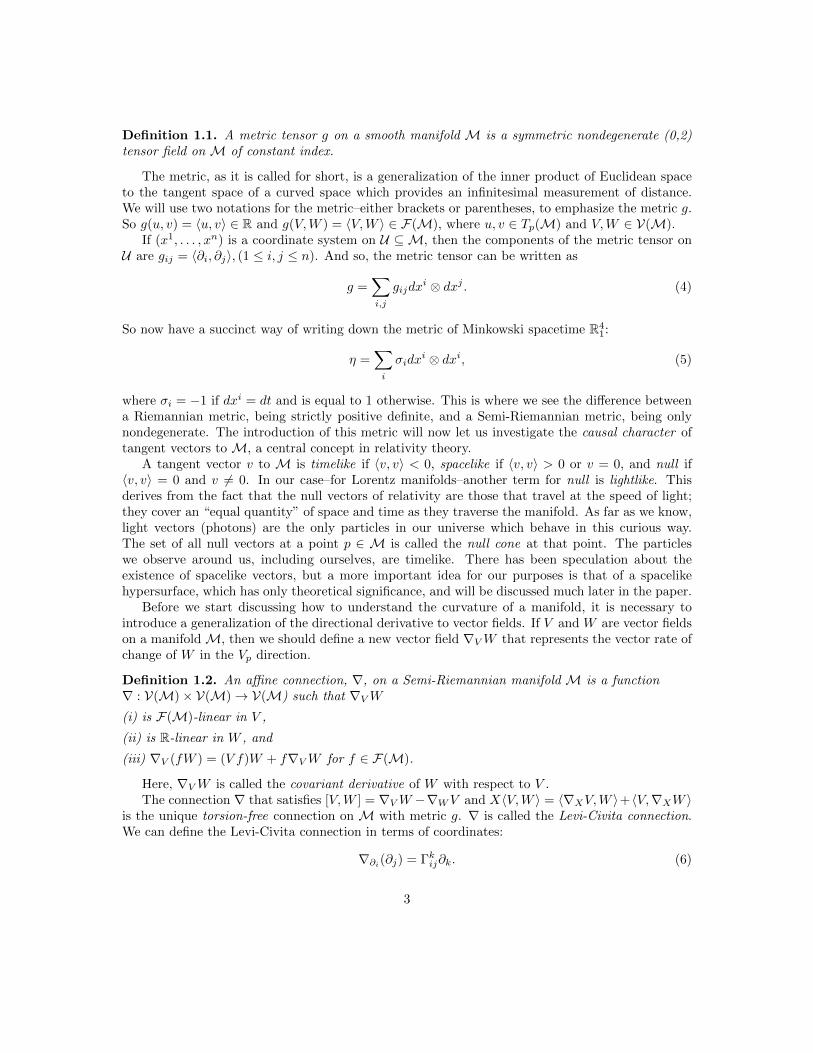
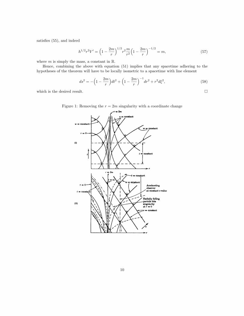
Figure 1: Removing the r = 2m singularity with a coordinate change

10

2.3 Singularities in Schwarzschild Spacetime

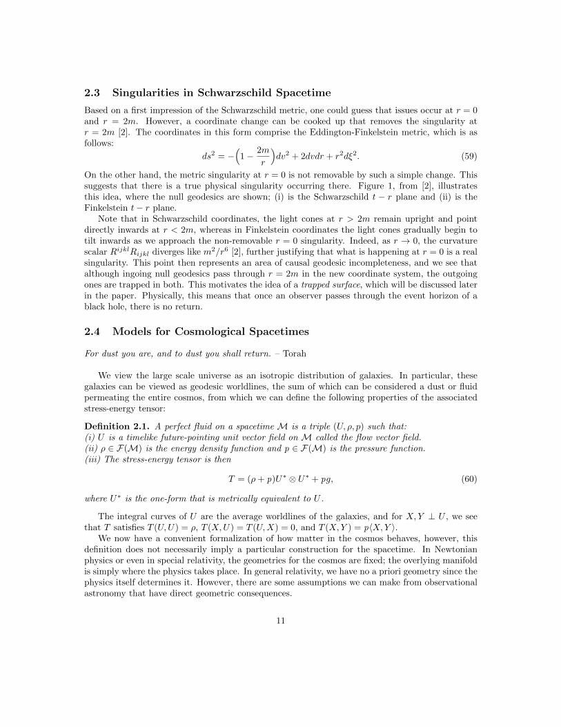
Based on a first impression of the Schwarzschild metric, one could guess that issues occur at r = 0and r = 2m. However, a coordinate change can be cooked up that removes the singularity atr = 2m [2]. The coordinates in this form comprise the Eddington-Finkelstein metric, which is asfollows:

ds2 = −(

1− 2m

r

)dv2 + 2dvdr + r2dξ2. (59)

On the other hand, the metric singularity at r = 0 is not removable by such a simple change. Thissuggests that there is a true physical singularity occurring there. Figure 1, from [2], illustratesthis idea, where the null geodesics are shown; (i) is the Schwarzschild t − r plane and (ii) is theFinkelstein t− r plane.

Note that in Schwarzschild coordinates, the light cones at r > 2m remain upright and pointdirectly inwards at r < 2m, whereas in Finkelstein coordinates the light cones gradually begin totilt inwards as we approach the non-removable r = 0 singularity. Indeed, as r → 0, the curvaturescalar RijklRijkl diverges like m2/r6 [2], further justifying that what is happening at r = 0 is a realsingularity. This point then represents an area of causal geodesic incompleteness, and we see thatalthough ingoing null geodesics pass through r = 2m in the new coordinate system, the outgoingones are trapped in both. This motivates the idea of a trapped surface, which will be discussed laterin the paper. Physically, this means that once an observer passes through the event horizon of ablack hole, there is no return.

2.4 Models for Cosmological Spacetimes

For dust you are, and to dust you shall return. – Torah

We view the large scale universe as an isotropic distribution of galaxies. In particular, thesegalaxies can be viewed as geodesic worldlines, the sum of which can be considered a dust or fluidpermeating the entire cosmos, from which we can define the following properties of the associatedstress-energy tensor:

Definition 2.1. A perfect fluid on a spacetime M is a triple (U, ρ, p) such that:(i) U is a timelike future-pointing unit vector field on M called the flow vector field.(ii) ρ ∈ F(M) is the energy density function and p ∈ F(M) is the pressure function.(iii) The stress-energy tensor is then

T = (ρ+ p)U∗ ⊗ U∗ + pg, (60)

where U∗ is the one-form that is metrically equivalent to U .

The integral curves of U are the average worldlines of the galaxies, and for X,Y ⊥ U , we seethat T satisfies T (U,U) = ρ, T (X,U) = T (U,X) = 0, and T (X,Y ) = p〈X,Y 〉.

We now have a convenient formalization of how matter in the cosmos behaves, however, thisdefinition does not necessarily imply a particular construction for the spacetime. In Newtonianphysics or even in special relativity, the geometries for the cosmos are fixed; the overlying manifoldis simply where the physics takes place. In general relativity, we have no a priori geometry since thephysics itself determines it. However, there are some assumptions we can make from observationalastronomy that have direct geometric consequences.

11

Most clearly, it seems to be the case that gravity attracts, on average. This is called thetimelike convergence condition, and can be expressed as Ric(v, v) ≥ 0 for all timelike vectors vtangent to M. In terms of the more physically tangible stress energy tensor, this is representedas T (v, v) ≥ 1

2C(T )〈v, v〉 for all timelike and null vectors v tangent to M, where C(T ) is themetric contraction of the stress-energy tensor T . T (v, v) is the energy density, and in this formthe condition is called the strong energy condition. We can conceive of matter configurations whichviolate this condition; for example, a cosmological inflationary process would do so. However, thecurrent state of our universe seems to adhere to it, so it is not an altogether dangerous assumption.A violation of this condition would imply that our current theory of general relativity would haveto be upgraded in some way.

The general form of these cosmological manifolds will be M = I × S, where I is a potentiallyinfinite interval in R and S is a connected three dimensional manifold. For the flow vector field U ,physical assumptions imply that 〈U,U〉 = −1. In addition, because the relative motion of galaxiesis negligible on a large scale, we have that U ⊥ S(t), where S(t) = t× S is a hypersurface servingas the common restspace for all of the galaxies at time t. Each of these slices is thus a Riemannianspacelike hypersurface which must have constant curvature C(t). With this in mind, we can definethe general form of our cosmological models as follows:

Definition 2.2. Let S be a connected three-dimensional Riemannian manifold of constant curvaturek = −1, 0, or 1, and let f > 0 by a smooth function on an open interval I ∈ R1

1. Then the warpedproduct

M(k, f) = I ×f S (61)

is called a Robertson-Walker (or Friedmann-Lemaıtre) spacetime.

Based on this construction, we see that S can be fundamentally categorized as H3,R3, or S3,since it must have constant curvature k = −1, 0, or 1. The metric thus takes the general form:

ds2 = −dt2 + f2(t)[dr2 + S2

k(r)dξ2], (62)

where the function Sk(r) is either hyperbolic, linear, or trigonometric, depending on k being −1, 0,or 1, respectively. Which geometry S adheres to in the physical universe is an active area ofresearch in both observational and theoretical cosmology. The discovery of this geometry wouldimply incredible facts about the initial and final conditions of our universe.

With this characterization of Robertson Walker spacetimes, we’ll try to deduce further propertieswith a few calculations.

Lemma 2.1. If V,W are in the lift of S to M(k, f) and taking U to be the flow vector field, in thelift of I, we have that nor∇VW = II(V,W ) = 〈V,W 〉(f ′/f)U .

Proof.

〈∇VW,U〉 = −〈W,∇V U〉 = −〈W, (Uff

)V 〉, (63)

given from the general form ∇VX = (Xff )V . Then we have that

−〈W, (Uff

)V 〉 = −(Uf

f)〈W,V 〉 = −〈gradf, U〉

f〈V,W 〉 =

f ′

f〈V,W 〉. (64)

12

Now that we have its components, we see that the mean curvature vector field is given as

II(V,W ) =f ′

f〈V,W 〉U. (65)

This will be a very useful result later on when we will be analyzing submanifold convergence interms of its mean curvature. Now we would like to see results for the Ricci curvature, given thatit is the primary object of interest in the Einstein field equations. We will simply list the formulasgiven in Chapter 12 of [1], as they are a simple application of the warped product formulas in theappendix.

Lemma 2.2. For M(k, f) with flow vector field U = ∂t and X,Y ⊥ U , we have

Ric(U,U) = −3f ′′

f(66)

and

Ric(X,Y ) =(

2(f ′

f)2 +

2k

f2+f ′′

f

)〈X,Y 〉. (67)

In addition, Ric(U,X) = Ric(U, Y ) = 0, and further contraction gives us

S = 6(

(f ′

f)2 +

k

f2+f ′′

f

). (68)

Finally, we want to make the above calculations compatible with our definition of the stress-energy tensor. Because the Einstein equation can be rearranged as T = 1

8π

(Ric − 1

2Sg), then acomparison with the definition of T with Lemma 2.2 quickly gives us

8πρ

3= (

f ′

f)2 +

k

f2(69)

−8πp =2f ′′

f+ (

f ′

f)2 +

k

f2. (70)

A further rearrangement stemming from a simple combination of the two above expressions givesus a relationship between the warping function and the energy density and pressure:

3f ′′

f= −4π(ρ+ 3p). (71)

In addition to these geometric results, astronomical observations have had influence on thededuction of the shape of the cosmos. For example, in 1927, Georges Lemaıtre theorized that theuniverse is expanding. Shortly thereafter in 1929, Edwin Hubble realized that the universe is indeedexpanding at a rate proportional to the Hubble constant H0 = f ′(t0)/f(t0) = (8± 2)× 10−9 years,where t0 is the current time. A more accurate name for this would be the Hubble parameter, becausefurther observation since 1929 has implied that the universe is expanding at an accelerating rate;however, it is sufficient for our purposes to consider it a constant. In particular, this fact impliesthat the restspaces S(t) are expanding, and so f ′ > 0. Astronomical data has also shown thatenergy density is significantly higher than pressure, that is, ρ >> p. With all of the above, we canjustify the existence of cosmological singularities.

13

2.5 Singular Points in the FLRW Models

To find singular points, we look at a simple result stemming from local linear approximations ofthe warping function f and see how this implies that f has a beginning some finite time ago.

Proposition 2.1. Let M(k, f) = I ×f S. If H0 > 0 for some t0 and ρ + p > 0, then I has aninitial endpoint t such that t0 −H−1

0 < t < t0.

Proof. Equation (71) shows us that ρ + p > 0 implies f ′′ < 0 and f > 0 everywhere up to thecurrent time t0. That is, the graph of f is concave down below its tangent line at t0. This line isthe graph of F (t) = f(t0)[1+H0(t−t0)]. In particular, F (t0−H−1

0 ) = f(t0)(1−1) = 0, and becausef remains concave down, as t approaches t0 −H−1

0 , it must be the case that f has a beginning atsome point t before then.

The future behavior of f is still under consideration in theoretical cosmology and will ultimatelyhelp us decipher if the universe continues to a big crunch or a big rip. However, the above resultjustifies that the past behavior of f implies the universe began a finite time ago, bounded byH−1

0 = 18 billion years. Very recent measurements of the cosmic microwave background radiationdue to the Planck space observatory have pinned the age of our universe at 13.82 billion years.Thus, we see that the cosmological models due to Friedmann, Lemaıtre, Robertson and Walkerthose many decades ago have come to some fruition.

This result, however, doesn’t say anything about the state of the universe at its beginning. If theenergy density ρ approaches infinity as t→ t, then we say that M(k, f) has a physical singularityat that time. An initial singularity is a big bang provided f → 0 and f ′ → ∞ as t goes to t. Afinal singularity is called a big crunch if f → 0 and f ′ → −∞ as t approaches a finite endpoint t.We now present a result that generalizes the preceding proposition into including the size behaviorof f , not just the finiteness of its parameter. The proof can be found in [1], but the diagram ofFriedmann models neatly summarizes the intuition.

Proposition 2.2. Assume that M(k, f) has only physical singularities and that I is maximal. IfH0 > 0 for some t0, ρ > 0, and if there exist constants a,A such that −1/3 < a ≤ p/ρ ≤ A, then:(i) The initial singularity is a big bang.(ii) If k = 0 or −1, then I = (t,∞) and as t→∞, f →∞ and ρ→ 0.(iii) If k = 1, then f reaches a maximum followed by a big crunch, hence I is a finite interval (t, t).

Like in the last proposition, we see that the future behavior of f is still not completely pre-dictable. However, this result does strongly imply that the universe began in an incredibly dense,high-energy state some finite time ago. Developing theories of dark matter and dark energy suggestthat a hyperbolic space is a much more likely candidate for the large scale structure of the universethan the spherical model. Additionally, further examination of the behavior of dark matter andenergy could eventually imply that Einstein’s general theory will have to be improved upon.

Finally, it is important to note here that all of our above assumptions about the cosmic structurecontain some sort of symmetry that is mathematically feasible, but physically unrealistic. This couldallow physicists to dismiss catastrophic phenomena like the big bang as a mathematical curiosityand not a real occurrence, given that the universe itself does not adhere strictly to such a highdegree of symmetry. This leads us to our next section, where we observe that singularities stillhappen, even under weaker geometric conditions.

14

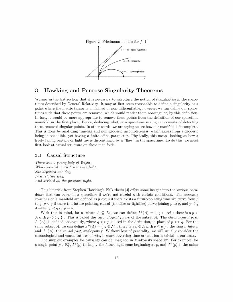
Figure 2: Friedmann models for f [1]

3 Hawking and Penrose Singularity Theorems

We saw in the last section that it is necessary to introduce the notion of singularities in the space-times described by General Relativity. It may at first seem reasonable to define a singularity as apoint where the metric tensor is undefined or non-differentiable, however, we can define our space-times such that these points are removed, which would render them nonsingular, by this definition.In fact, it would be more appropriate to remove these points from the definition of our spacetimemanifold in the first place. Hence, deducing whether a spacetime is singular consists of detectingthese removed singular points. In other words, we are trying to see how our manifold is incomplete.This is done by analyzing timelike and null geodesic incompleteness, which arises from a geodesicbeing inextendible, yet having a finite affine parameter. Physically, this means looking at how afreely falling particle or light ray is discontinued by a “flaw” in the spacetime. To do this, we mustfirst look at causal structure on these manifolds.

3.1 Causal Structure

There was a young lady of WightWho travelled much faster than light.She departed one day,In a relative way,And arrived on the previous night.

This limerick from Stephen Hawking’s PhD thesis [4] offers some insight into the various para-doxes that can occur in a spacetime if we’re not careful with certain conditions. The causalityrelations on a manifold are defined as p << q if there exists a future-pointing timelike curve from pto q, p < q if there is a future-pointing causal (timelike or lightlike) curve joining p to q, and p ≤ qif either p < q or p = q.

With this in mind, for a subset A ⊆ M, we can define I+(A) = q ∈ M : there is a p ∈A with p << q . This is called the chronological future of the subset A. The chronological past,I−(A), is defined analogously, where q << p is used in the definition, in place of p << q. For thesame subset A, we can define J+(A) = q ∈ M : there is a p ∈ A with p ≤ q , the causal future,and J−(A), the causal past, analogously. Without loss of generality, we will usually consider thechronological and causal futures of sets, because reversing time orientation is trivial in our cases.

The simplest examples for causality can be imagined in Minkowski space Rn1 . For example, fora single point p ∈ Rn1 , I+(p) is simply the future light cone beginning at p, and J+(p) is the union

15

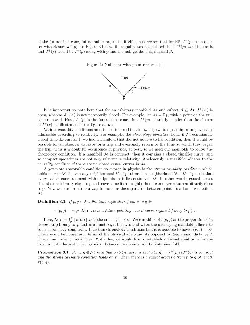
of the future time cone, future null cone, and p itself. Thus, we see that for Rn1 , I+(p) is an openset with closure J+(p). In Figure 3 below, if the point was not deleted, then I+(p) would be as isand J+(p) would be I+(p) along with p and the null geodesic rays α and β.

Figure 3: Null cone with point removed [1]

It is important to note here that for an arbitrary manifold M and subset A ⊆ M, I+(A) isopen, whereas J+(A) is not necessarily closed. For example, let M = R2

1, with a point on the nullcone removed. Here, I+(p) is the future time cone , but J+(p) is strictly smaller than the closureof I+(p), as illustrated in the figure above.

Various causality conditions need to be discussed to acknowledge which spacetimes are physicallyadmissible according to relativity. For example, the chronology condition holds if M contains noclosed timelike curves. If we had a manifold that did not adhere to his condition, then it would bepossible for an observer to leave for a trip and eventually return to the time at which they beganthe trip. This is a doubtful occurrence in physics, at best, so we need our manifolds to follow thechronology condition. If a manifold M is compact, then it contains a closed timelike curve, andso compact spacetimes are not very relevant in relativity. Analogously, a manifold adheres to thecausality condition if there are no closed causal curves in M.

A yet more reasonable condition to expect in physics is the strong causality condition, whichholds at p ∈ M if given any neighborhood U of p, there is a neighborhood V ⊂ U of p such thatevery causal curve segment with endpoints in V lies entirely in U . In other words, causal curvesthat start arbitrarily close to p and leave some fixed neighborhood can never return arbitrarily closeto p. Now we must consider a way to measure the separation between points in a Lorentz manifoldM.

Definition 3.1. If p, q ∈M, the time separation from p to q is

τ(p, q) = sup L(α) : α is a future pointing causal curve segment from p to q .

Here, L(α) =∫ qp| α′(s) | ds is the arc length of α. We can think of τ(p, q) as the proper time of a

slowest trip from p to q, and as a function, it behaves best when the underlying manifold adheres tosome chronology conditions. If certain chronology conditions fail, it is possible to have τ(p, q) =∞,which would be nonsense in terms of the physical analogue. As opposed to Riemannian distance d,which minimizes, τ maximizes. With this, we would like to establish sufficient conditions for theexistence of a longest causal geodesic between two points in a Lorentz manifold.

Proposition 3.1. For p, q ∈M such that p << q, assume that J(p, q) = J+(p)∩J−(q) is compactand the strong causality condition holds on it. Then there is a causal geodesic from p to q of lengthτ(p, q).

16

Proof. Let αn be a sequence of future pointing causal curve segments from p to q such that thelengths converge to τ(p, q), which will have finite length because of the strong causality condition.Because J(p, q) is the smallest set containing all future pointing causal curves from p to q, all αn arecontained within J(p, q). Because J(p, q) is compact and adheres to the strong causality condition,there is a causal broken geodesic γ from p to q such that L(γ) = τ(p, q). If γ has breaks, then thereis a longer causal curve from p to q, but τ is a maximizing function, meaning that γ is unbroken.

This proposition alludes to a nice feature of spacetimes with a very convenient and physicallyrealistic structure. We define it as follows:

Definition 3.2. A subset U ⊆ M is globally hyperbolic given that the strong causality conditionholds on U , and if p, q ∈ U such that p < q, then J(p, q) is compact and contained in U .

By this definition and the preceding proposition, for all p, q ∈ U such that U is globally hy-perbolic, there is a causal geodesic joining the two points. If the entire manifold M is globallyhyperbolic, then all sets J+(p), J−(q), and J(p, q) are closed.

Examples of globally hyperbolic spaces are Minkowski spacetime, Robertson-Walker spacetimesand Schwarzschild spacetime. Thus, it is apparent that global hyperbolicity will play an importantrole in our analysis of singular spacetimes. Looking at the causal behavior of subsets and subman-ifolds is also necessary for finding singularities in a parent manifold, so we have the following:

Definition 3.3. A subset A ⊆ M is achronal if p << q never holds for any p, q ∈ A. In otherwords, no timelike curve in M meets A more than once.

The simplest example of an achronal set would be a hyperplane t constant in Minkowski space.In addition, this hyperplane has the additional feature of being edgeless. The edge of an achronalset A consists of all points p ∈ A such that every neighborhood U of p contains a timelike curvefrom I−(p,U) to I+(p,U) that does not meet A.

3.2 Spacelike Hypersurfaces

We now inspect achronal sets with a more continuous structure, viewing them as surfaces withfeatures that help us deduce the existence of singularities in the overlying spacetime.

Definition 3.4. A subspace S ⊂ T , where T is an n-dimensional topological manifold, is a topo-logical hypersurface provided that for each p ∈ S, there is a neighborhood U of p in T and ahomeomorphism φ of U onto an open set in Rn such that φ(U ∩ S) = φ(U) ∩ Π, where Π is ahyperplane in Rn.

An achronal set A is a topological hypersurface if and only if A and edge A are disjoint.Additionally, A being a closed topological hypersurface is equivalent to edge A being empty. Asignificant example of a closed topological hypersurface is ∂J+(p) ⊂ R4

1, the null cone at a pointp ∈ R4

1.An important class of achronal hypersurfaces in Lorentzian geometry are Cauchy hypersurfaces,

which represent an “instant in time” in the entire spacetime.

Definition 3.5. A Cauchy hypersurface (or simply Cauchy surface) S ⊂M is a subset that is metexactly once by every inextendible causal curve in M.

17

The null cone discussed above would then not be an example of a Cauchy hypersurface, but thehyperplanes t constant, as subsets of R4

1, would be. A spacetime that contains a Cauchy hypersurfaceis globally hyperbolic, so it’s clear that not all spacetimes admit a Cauchy hypersurface. Thepreceding example shows that R4

1 admits one, but removing any one point takes away this property.The important idea behind a Cauchy hypersurface is that the initial conditions on such a surfacedetermine observable data on all of the spacetime. This notion leads us to ask about what areas inthe spacetime depend directly on a particular spacelike slice.

Definition 3.6. If A ⊆ M is achronal, then the future Cauchy development of A is the set of allpoints p ∈ M such that every past inextendible causal curve through p meets A. We denote it asD+(A).

In a physical sense, D+(A) is the part of A’s causal future that is predictable from A. No pastintextendible curve can enter D+(A) without first having passed through A. Another name forD+(A), more common with physicists, is the future domain of dependence of A. Dually, D−(A) isdefined to be the set of all points p ∈ M such that every future inextendible causal curve throughp meets A. In other words, D−(A), the past Cauchy development of A, is the past domain ofdependence of A. Every timelike curve passing through D−(A) will also pass through A. We willrefer to the union of the future and past Cauchy developments, D(A) = D+(A) ∪D−(A), simplyas the Cauchy development of A.

A significant fact is that A is a hypersurface such that D(A) =M if and only if A is a Cauchyhypersurface. This particular view of what it means to be a Cauchy hypersurface makes it clear howinitial conditions on the surface define solutions of its evolution throughout the entire spacetime.We now want to prove a lemma which uses these definitions and is useful later, but we first mustintroduce a definition that is a useful tool in causal set theory

Definition 3.7. Let αn be an infinite sequence of future-pointing causal curves in M, and let Rbe a convex covering of M. A limit sequence for αn relative to R is a finite or infinite sequencep = p0 < p1 < . . . in M such that

(i) For each pi, there is a subsequence αn and, for each m, numbers sm0 < sm1 < . . . < smi suchthat (a) limm→∞ αm(smj ) = pj for each j ≤ i, and (b) for each j < i, the points pj , pj+1 and thesegments αm|[smj , smj+1

] for all m are contained in a single set Cj ∈ R.

(ii) If pi is infinite, it is nonconvergent. If pi is finite, then it has more than one point and nostrictly longer sequence satisfies (i).

The existence of a limit sequence is insured by two mild conditions on αn, namely (1): thesequence αn(0) converges to a point p, and (2): there is a neighborhood of p that contains onlyfinitely many of the αn. If pi is a limit sequence for αn, we let λi be the future pointing causalgeodesic from pi to pi+1 in a convex set Ci, as in (i). Joining these together gives us a brokengeodesic λ =

∑λi called a quasi-limit of αn, which has vertices pi. If pi is infinite, then it is

nonconvergent, by definition, and so λ is future inextendible.

Lemma 3.1. Let A be an achronal set. If p ∈ D+(A) − I−(A), then J−(p) ∩D+(A) is compact.

Proof. Because taking p ∈ A consists of dealing with p alone, we assume that p ∈ I+(A) ∩D(A).Now, we let xn be an infinite sequence in J−(p) ∩D+(A) and let αn be a past-pointing causalcurve segment from p to xn. If there is a subsequence of xn converging to p, then we are done, sowe assume otherwise. Hence, there must be a past directed limit sequence pi for αn starting

18

at p. If pi is infinite, then it is nonconvergent, by the definition of a limit sequence, so for somen, there will be an xn ∈ I−(A), which is a contradiction. Given that pi is finite, there must besome subsequence xm which converges to a point x ∈ J−(p). Let σ be a timelike curve fromp+ ∈ D+(A) ∩ I+(p) to x. If σ passes through A, then either x ∈ A ⊂ D+(A) or x ∈ I−(A), thelatter implying that there is some xn ∈ I−(A), which would be a contradiction, so x ∈ D+(A). If σdoes not pass through A, then we get that x ∈ D+(A). Either way, x ∈ J−(p) ∩D+(A), meaningthat xn converges to a point in J−(p) ∩ D+(A), which then must be closed. Because it also isbounded, it must hence be compact.

Thus far, we have discussed the above objects in mostly topological terms, however, we havenoted that they can be considered manifolds with a Lorentzian structure, where the initial surfacedata is smooth. Thus, we treat these hypersurfaces as submanifolds, and use results from Appendix4.1 to deduce their properties.

Lemma 3.2. Let S be a closed achronal spacelike hypersurface inM. If q ∈ D+(S)−S, then thereexists a geodesic γ from S to q such that L(γ) = τ(S, q). Moreover, γ is normal to S and has nofocal points of S before q.

Proof. We take it as a given that because S is a closed achronal hypersurface, that D(S) is globallyhyperbolic. Hence, by Lemma 3.1, J−(q)∩D+(S) is compact. This then implies that J−(q)∩ S iscompact, and because it is also globally hyperbolic, the time separation function must be continuouson it. Hence, it achieves a maximum at, say, p. This maximum must then be τ(p, q) = τ(S, q). ByProposition 3.1, there is then a causal geodesic γ from p to q such that L(γ) = τ(S, q). Becauseq ∈ D+(S) − S, τ(S, q) > 0, meaning that γ is timelike. Hence, γ is normal to S. In addition,Proposition 5.2 in the appendix guarantees there will be no focal points along γ.

Because the same theorem holds for D−(S), this result holds for the entire Cauchy development,D(S). This leads us to look at cases of spacetimes where the entire future or past of a hypersurfacecannot be deduced from the data on the surface. Previously, we mentioned that removing a pointfrom R4

1 would imply it does not contain a Cauchy hypersurface, and now we generalize this withthe idea of a Cauchy horizon.

Definition 3.8. If A is an achronal set, then the future Cauchy horizon is H+(A) = p ∈ D+(A) :I+(p) does not meet D+(A) .

Intuitively, H+(A) marks the future limit of the spacetime region that can be predicted from A.For example, if we let S ⊂ R4

1 be the hyperplane 0 constant, then removing a point p >> 0 wouldmake it so that H+(S) = ∂J+(p). That is, events in J+(p) need not necessarily be influenced bydata from S.

With H−(A) defined dually, we have H(A) = H+(A) ∪ H−(A). Note that for a spacelikehypersurface S, if H(S) is empty, then D(S) =M, meaning that S is a Cauchy hypersurface. Thereverse implication is also true. We now state a proposition that shows the relationship betweenCauchy horizons and other causal structures, along with describing generators of the set.

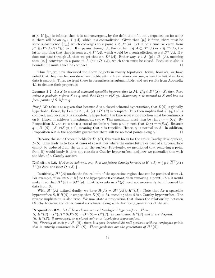
Proposition 3.2. Let S be a closed acausal topological hypersurface. Then:(i) H+(S) = I+(S) ∩ ∂D+(S) = D+(S)−D+(S). In particular, H+(S) and S are disjoint.(ii) H+(S), if nonempty, is a closed achronal topological hypersurface.(iii) Starting at each q ∈ H+(S), there is a past-inextendible null geodesic without conjugate pointsthat is entirely contained in H+(S). These geodesics are the generators of H+(S).

19

Figure 4: Deleting a point p from the domain of dependence of a spacelike surface Σ generates aCauchy horizon [5]

The proof is a lengthy exercise in causal set theory, but inspecting a simple example providesenough intuition to understand the result, considering the definitions. In Figure 4, the generatorsof the future Cauchy horizon of the surface are the straight lines emanating from p that comprise∂J+(p). It is also clear from the picture that ∂D+(Σ) minus D+(Σ) itself is the future Cauchyhorizon.

With all of the causal structure we have introduced, and after analyzing conditions for theexistence of causal geodesics and focal points of submanifolds, we are now prepared to examine thesingularity theorems.

3.3 Hawking’s Singularity Theorem

Here, we want to generalize what we discussed in the section on FLRW spacetimes. Analysis onthose metrics led us to the conclusion that a singularity must exist somewhere in the finite past.However, it is easy for physicists to dismiss these singularities as simply mathematical phenomenastemming from the fact that those metrics are highly symmetric. In physical terms, even thoughspace seems approximately isotropic, it may not be necessarily be so enough to cause catastrophicsingularities in the past. In the case of the singularity theorems, we can say that a spacetimeis only approximately FLRW (thus more physically realistic), but still must contain singularitiesunder these weaker geometric conditions.

We know that a spacelike slice t × S in a Robertson-Walker spacetime is a closed topologicalhypersurface, and the fact that every inextendible null geodesic must meet it implies that H(t×S)is empty. Hence, this slice is a Cauchy hypersurface. In addition, observational astronomy hashelped us deduce that on the spacelike slice of present time, all galaxies are diverging from oneanother at an accelerating rate, implying past convergence. Because we assume gravity on averageattracts, that is, Ric(v, v) ≥ 0, all of this implies that past-directed timelike curves starting in thespacelike slice are incomplete. The concept of conjugate points, and thus focal points, is criticalhere because they determine where a timelike geodesic fails to be a local maximizer of proper timeand where a null geodesic fails to remain on the future boundary of a point.

We state the results in future terms, to remain consistent with our trend. We now prove two ofHawking’s singularity theorems, the first being stronger, but assuming more.

20

Theorem 3.1. Suppose that Ric(v, v) ≥ 0 for all timelike tangent vectors v to a Lorentzian manifoldM. Also, let S be a spacelike future Cauchy hypersurface with future convergence k ≥ b > 0. Thenevery future-pointing timelike curve starting in S must have length at most 1

b .

Proof. We assume that q ∈ D+(S) − S. By Lemma 3.2, there must exist a timelike, normalgeodesic γ from S to q such that it contains no focal points before q and L(γ) = τ(S, q). However,our assumptions imply that Ric(γ′, γ′) ≥ 0, and because S has convergence k ≥ b > 0, Proposition5.2 in the appendix implies that there will be a focal point of S along γ before q if L(γ) > 1

b . Thus,D+(S) ⊆ p ∈ M : τ(S, p) ≤ 1

b . Because S is a future Cauchy hypersurface, H+(S) is empty.The definition of H+(S) and S being a future Cauchy hypersurface then directly imply that allp ∈ M are such that I+(p) meets D+(S). Because this is the case for all p ∈ M, we must havethat I+(S) ⊆ D+(S) ⊆ p ∈ M : τ(S, p) ≤ 1

b . That is to say, every future-pointing timelikecurve in S must have length at most 1

b .

The strongest assumption that we make here is thatM contains a future Cauchy hypersurface.Our universe being approximately FLRW makes this a reasonable assumption to make. However,future developments in physics can disprove the validity of this assumption, so it would be nice totest for timelike incompleteness under more general circumstances.

Theorem 3.2. Suppose that Ric(v, v) ≥ 0 for all timelike tangent vectors v to M. Additionally,let S be a connected, compact spacelike hypersurface with future convergence k > 0. Then M isfuture timelike incomplete.

Proof. Let b be the minimum value of k on S, which exists because S is compact. We want toprove a weaker conclusion than the previous theorem, namely, (i) that there exists an inextendiblefuture-pointing normal geodesic γ starting at S with length bounded by 1

b , which would imply thatM is future timelike incomplete. Without loss of generality, we can assume that S is achronal. Asin the previous theorem, this gives us that D+(S) ⊆ p ∈ M : τ(S, p) ≤ 1

b . Now, we assumethat H+(S) 6= ∅, because otherwise the previous proof holds and we are done. We also assumethat (i) is false, to derive a contradiction. With this, we prove (ii) if q ∈ H+(S), then there existsa normal geodesic γv from S to q such that L(γv) = τ(S, q) ≤ 1

b .

Proof. In the normal bundle of S, let B be the set of all zero vectors and future-pointing vectorsv such that |v| ≤ 1

b . Because S is compact, B must be so as well, meaning that there exists asequence qn in D+(S) such that qn → q. For each qn, we know there exists a normal geodesicγvn from S to qn such that L(γvn) = τ(S, q) ≤ 1

b . Hence, for each qn, there exists a vn ∈ B suchthat exp(vn) = qn. Because B is compact, vn has a limit v ∈ B, and then by continuity, thismeans that qn has the limit exp(v), i.e. exp(v) = q. In addition, we have |vn| → |v| ≤ 1

b andτ(S, qn) = |vn|. Because the time separation function is lower semi-continuous, |v| ≥ τ(S, q). Now,because we assumed that (i) is false, this means that γv from S to q is defined on [0, 1] with length|v|, i.e. τ(S, q) = |v| ≤ 1

b , finishing the proof.

We can now assume by Proposition 3.2 that (iii) the time separation function p → τ(S, p) isstrictly decreasing on past-pointing generators of H+(S). Let α be such a generator. Within thedomain of its parameterization, assume that s < t. By (ii), there is a past-pointing timelike geodesicσ for α(t) to S such that L(σ) = τ(S, α(t)). Because α is a null curve, by definition, the causalcurve α|[s, t] + σ is broken and hence can be lengthened by a fixed endpoint deformation. Thus,we have τ(S, α(s)) > L(α|[s, t] + σ) = L(σ) = L(S, α(t)). Because we assumed that (i) is false, the

21

normal exponential map is defined on all of B, implying then that H+(S) is compact as a subset ofthe continuous image of B. The time separation is lower semi-continous, so its restriction to H+(S)achieves a minimum somewhere. This contradicts (iii) because there is a generator extending intothe past from each point of H+(S). So M is future timelike incomplete.

With this theorem, we weaken the first one significantly, but still preserve the fact that M isfuture timelike incomplete.

When the time orientation of these theorems is reversed, we recover the past singularities thatarose in Propositions 2.1 and 2.2, but without the need for exact spatial isotropy. This is particularlyappealing, given that recent observations of the cosmic microwave background radiation have shownit to be anisotropic. We can also weaken the assumptions slightly by requiring only that Ric(γ′, γ′) ≥0 for normal geodesics γ to S. In this case, Ric(γ′, γ′) ≥ 0 is equivalent to our very reasonablephysical assumption that ρ+ 3p ≥ 0. From Lemma 2.1, we have that each spacelike slice has mean

curvature f ′(t0)f(t0) U , and so the submanifold convergence is k = − f

′(t0)f(t0) . Thus, we see that Hubble

expansion at time t0 is equivalent to S(t0) having convergence k ≤ b < 0, and if these slices areCauchy hypersurfaces, then Theorem 3.1 holds. Deleting a closed set from I+(S) would renderTheorem 3.1 inapplicable, but Theorem 3.2 will continue to hold because S remains compact.

3.4 Penrose’s Singularity Theorem

The result which motivated Stephen Hawking’s investigation of Big Bang singularities was thatof Roger Penrose concerning “black hole” singularities. The idea is analogous to the previoustheorems: under slightly less symmetric conditions, it is still the case that a collapsing star producesa singularity at r = 0. This is suggested by the analyses in section 2.3, but now we want to generalizethose ideas by looking at a spacelike submanifold P ⊆ M and investigating its convergence, as inthe previous section.

If P is a spacelike submanifold of codimension ≥ 2 and if H is its mean curvature vector field,then the following are equivalent: (1) k(v) = 〈H, v〉 > 0 for all future-pointing null vectors v normalto P, (2) k(w) = 〈H,w〉 > 0 for all future-pointing causal vectors w normal to P, and (3) H ispast-pointing timelike [1]. This motivates the following significant definition.

Definition 3.9. A spacelike submanifold P ⊆M is future-converging, i.e. a trapped surface, if itsmean curvature vector field H is past-pointing timelike.

In the case of a sphere S2(r) of constant time inside a Schwarzschild black hole, the meancurvature vector field is H = −gradr/r. Then

k(v) = 〈H, v〉 = 〈−gradr

r, v〉 =

−v(r)

r, (72)

and so we see that H is past-pointing timelike, since v is defined to be a future pointing null vector.In particular, this means that S2(r) is a trapped surface.

In terms of our language of causal set theory, we want an analogous idea of a set being “trapped.”

Definition 3.10. Let E+(A) = J+(A) − I+(A). If A is a closed achronal subset of M and ifE+(A) is compact, then A is future-trapped.

Note that E+(A) is generated by conjugate-free null geodesics. With this, we would like to seewhen being a trapped subset coincides with being a trapped surface; this will tell us somethingabout the existence of singularities. First, we must introduce a lemma.

22

Lemma 3.3. Assume that:(1) Ric(v, v) ≥ 0 for all null tangent vectors v to M,(2) M is future null complete.Then if P is a compact achronal spacelike submanifold of codimension 2 that is future converging,then P is future-trapped.

The proof is contained in [1], and is completed by deducing that E+(P) is a compact topologicalmanifold. We are able to hide the background calculations concerning focal points by classifyingfuture converging submanifolds as trapped surfaces, and we will state the result in positive termsto see how dropping certain assumptions will “break” timelike completeness.

Theorem 3.3. Assume that:(1) Ric(v, v) ≥ 0 for all null tangent vectors v to M,(2) M contains a Cauchy hypersurface S,(3) P is a future-trapped, compact achronal spacelike submanifold of codimension 2,(4) M is future null complete.Then E+(P) is a Cauchy hypersurface in M.

Proof. Because M contains a Cauchy hypersurface, it must be globally hyperbolic, which immedi-ately implies that J+(p) is closed for all p ∈ M. The assumption that P is compact then meansthat J+(P) is closed. Because J+(P) = I+(P), we have that E+(P) = ∂J+(P). Hence, E+(P)is a topological manifold, and is thus compact by the preceding lemma.

For the given Cauchy hypersurface S, let ρ : E+(P)→ S be the restriction to S of a retraction.ρ is defined to be continuous then, and since E+(P) is achronal, the uniqueness of integral curvesimplies that ρ is an injective function. Hence, ρ is a homeomorphism of E+(P) to an open subset ofS. Because E+(P) is compact, ρ(E+(P)) must be compact, and thus closed in S. Then because S isconnected, it must be the case that ρ(E+(P)) = S. In other words, E+(P) and S are homeomorphicby ρ.

Now, let β be an inextendible timelike curve inM. We must show that it meets E+(P). Becausewe assumed thatM is time-oriented, it must be the case that β is locally an integral curve of sometimelike vector field X ∈ V(M). Because the strong causality condition holds, this can be extendedover M so that the retraction induced by X is a homeomorphism between E+(P) and S. Hence,because β meets S, it must also meet E+(P), meaning that it is a Cauchy hypersurface in M.

Corollary 3.1. If we assume that (1), (2) and (3) hold, but also that S is not compact, then M isfuture null incomplete.

Proof. Since S is not compact, but is still homeomorphic to E+(P), E+(P) is also not compact.This means that P cannot be future trapped, and also that S cannot be a Cauchy hypersurface,which is a contradiction and hence M cannot be future null complete.

Corollary 3.2. If (1), (2) and (3) hold, but if there is an extendible causal curve which does notpass through E+(P), then M is future null incomplete.

Proof. Because there is an inextendible causal curve not meeting E+(P), E+(P) is not a Cauchyhypersurface. In particular, H+(E+(P)) is non-empty. But E+(P) and S are homeomorphic bythe induced retraction from X ∈ V(M), and so H+(S) is also non-empty. This is a contradictionwith (2). Hence, M is future null incomplete.

These results generalize the existence of singularities within collapsing stars, even if they do notadhere to the perfect symmetry of the Schwarzschild solution.

23

4 Thoughts and questions

In the further development of established theories and in the forging of new ones, it may be appro-priate to consider the traceless part of the Riemann curvature tensor. This is known as the Weylcurvature tensor, and its components in covariant form are as follows [2]:

Cijkl = Rijkl +2

n− 2

(gi[lRk]j + gj[kRl]i]

)+

2

(n− 2)(n− 1)Sgi[kgl]j , (73)

where n is the dimension of the spacetime and the brackets in the subscripts represent 1/m! timesthe alternating sum of the enclosed indices, where m is the number of indices being permuted.The Weyl tensor represents the gravitational degrees of freedom, thus describing the tidal forcesinduced by a spacetime’s curvature. The stress-energy tensor Tij is analogous to the charge-currentvector Jµ in Maxwell’s electromagnetic theory. Similarly, the Weyl tensor Cijkl is analogous to thefield strength tensor Fµν , which is also a traceless quantity, describing the degrees of freedom ofthe electromagnetic field. Given that Fµν plays a crucial role in quantum field theory, it would beapt to consider the importance of the Weyl tensor in future gravitational theory. In addition, inempty space, the spacetime curvature is entirely Weyl curvature, so we see that it is responsiblefor the traversal of gravitational radiation through that empty space. This is of particular interest,considering the recent confirmation of the existence of gravitational waves by LIGO.

An important use for the Weyl tensor could perhaps be in a quantized theory of gravity. Forexample, given that the Weyl tensor is a conformal invariant, physicist Dr. Philip Mannheim hasmade use of it in his theory of conformal gravity, where he describes gravity as being quantizedsolely as a result of it being coupled with a quantized matter source [8]. By using an action ofconformal form, with the Weyl tensor, as opposed to the Einstein-Hilbert action, Dr. Mannheimjustifies that the EFE as we know them are sufficient to give the Schwarzschild solution, but notnecessary, allowing for a different equation of motion. In addition, he uses a PT-symmetric asopposed to a Hermitian quantum theory, to make the parts of this theory of quantized gravitycome together. The struggle to unify gravity with quantum theory has been on the frontier ofongoing research among theoretical physicists and mathematicians for the past century. WhetherWeyl curvature or such a refined quantum theory will play an important role in updating Einstein’stheory remains to be seen, however it is most certainly the case that the insight which providesthe missing link between different mathematical theories that describe the universe will come fromconcepts familiar to us, but that we have not yet fully considered.

Another topic in which the Weyl tensor garners attention is in Roger Penrose’s Weyl curvaturehypothesis. A characteristic feature of the Friedmann-Lemaıtre-Robertson-Walker spacetimes weexamined earlier is that their Weyl curvature vanishes identically. So let’s consider a universeevolving from an initial “Big Bang” state of uniform matter distribution. The hypothesis is that thiscorresponds to the primary source of curvature being Ricci curvature, whereas the Weyl curvatureis effectively zero [7]. As the spacetime evolves, the initially uniform matter distribution begins toclump together sporadically, and those clumps become sources of Weyl curvature. Given enoughtime, in some cases, these clumps become black holes, in which the Weyl curvature diverges. Inmore physical terms, the initial Big Bang singularity has a very low entropy, whereas the final blackhole singularities have a very high entropy. This geometric hypothesis would constrain the cosmosso that it adheres to the Second Law of Thermodynamics and closely resembles the FLRW models.This leads us to ask how the Weyl curvature tensor and other purely geometric concepts coulddecide further developments in gravitational theory, both in terms of explaining some mysteriouslarge scale phenomena and in the unification of gravity with quantum theory.

24

A development which has attracted curiosity ever since Einstein’s original 1915 publication hasbeen that of a cosmological constant, Λ. If we assume that it is non-zero, as some recent observationsmight imply, then the EFE take the form:

G+ Λg = 8πT. (74)

Originally, although he proposed its existence to constrain the universe to a static state, Einsteindismissed the cosmological constant quickly when it was discovered that the universe was expanding.Now, with recent observations implying an accelerating expansion of the universe, the cosmologicalconstant has been brought up again as a possible explanation, along with dark energy/matter.Perhaps there is yet a more purely geometric explanation for the accelerating expansion of theuniverse, where the need for strange physical assumptions like that of dark energy or even thereinstatement of the cosmological constant may be deemed superfluous. Indeed, one particular ideawhich has strongly grabbed my attention during the writing of this thesis is the Ricci flow. Thisis a geometric flow where the metric of a manifold changes in accordance with its Ricci curvature,defined by the partial differential equation:

∂tgij = −2Rij , (75)

where the t−parameter does not correspond with the time coordinate of a spacetime, but ratherparameterizes the individual metric components to change with t. It is generally defined in this waybecause it is typically done on a Riemannian (i.e. positive definite) metric. Examples of Ricci flowwould be a spherical manifold shrinking away in finite time because it has positive curvature, a flatmanifold remaining static because it has zero curvature and a hyperbolic manifold diverging due toits negative curvature. The concept of Ricci flow is one that I hope to do more research on, not onlybecause of its own merit, but also to see how it could be used in gravitational theory. In particular,rigging a Lorentz metric with Ricci flow may prove interesting, given that it is not a positive definitemetric. Perhaps its implementation to cosmological spacetimes could provide an explanation forphenomena we do not yet fully understand, like cosmic inflation and the accelerating expansion ofthe universe. Other ideas, like the mean curvature flow, are also of interest to me for these reasons.

One of the most relevant current issues with respect to the primary concepts introduced in thisthesis are the strong and weak cosmic censorship conjectures. The intuitive idea behind the SCCconjecture, as it is called for short, is that causal geodesic incompleteness is always accompaniedby divergence of the spacetime’s curvature. The WCC conjecture speculates that spacetime sin-gularities are not visible to far-away observers, i.e. there are no naked singularities. The mostprevalent solutions to the EFE, as we have seen, are singular, so it is appropriate to characterizethese singularities in some way. More formal statements of the conjectures are as follows [9]:

Conjecture 4.1 (Strong Cosmic Censorship). Globally hyperbolic spacetime solutions of the EFEcannot generically be extended as solutions past a Cauchy horizon.

Conjecture 4.2 (Weak Cosmic Censorship). In generic asymptotically flat solutions to the EFE,singularities are contained within a black hole event horizon.

It is important to note that the existence of spacetimes with Cauchy horizons does not disprovethe SCC conjecture nor does the existence of asymptotically flat spacetimes with singularities to thecausal past of far-away observers disprove the WCC, as stated in Dr. Jim Isenberg’s paper [9]. Thisfact makes it clear exactly how difficult it can be to prove or disprove these conjectures. However,these and other issues mentioned earlier remain as some of the most pertinent and fascinatingproblems in mathematical relativity, providing us with enough motivation for further study.

25

5 Appendix

5.1 Index Form, Focal Points, and Submanifold Convergence

In this section, we introduce results from the calculus of variations on manifolds that will be usefulfor the Hawking and Penrose singularity theorems. This section will not be self-contained; importantproofs will be covered, but many results will be taken as granted from O’Neill’s Semi-RiemannianGeometry [1].

Definition 5.1. A variation of a curve segment α : [a, b] → M is a two-parameter mappingx : [a, b]× (−δ, δ)→M such that α(u) = x(u, 0) for all a ≤ u ≤ b.

Now, for each v ∈ (−δ, δ), we let Lx(v) be the length of the longitudinal curve u 7→ x(u, v).So then Lx(0) = L(α). From now on, we will write Lx(v) = L(v), which won’t be misleadingconsidering the context. Our focus concerning the application of these tools will be to the secondvariation formula, which provides us with a link between geodesics and curvature.

We will take it as a given that a piecewise smooth curve segment α of constant speed c > 0 isan unbroken geodesic if and only if the first variation of arc length is zero for every fixed endpointvariation of α. The second variation, L′′(0), is needed only when L′(0) = 0, so, considering thepreceding fact, we need a formula for the second variation when our curve is a geodesic. Thevector field V (u) = xv(u, 0) gives the velocities for the transverse curves of x as they cross α andA(u) = xvv(u, 0) gives the accelerations. Note that if |α′| > 0, then any vector field Y on α splitsinto Y T + Y ⊥, its tangent and normal components to α. We now introduce the general expressionfor the second variation, called Synge’s Formula. The proof and some further implications are in[1].

Theorem 5.1. Let σ : [a, b] → M be a geodesic segment of speed c > 0 and sign ε. If x is avariation of σ, then

L′′(0) =ε

c

∫ b

a

[〈V ′⊥, V ′⊥〉 − 〈RV σ′V, σ′〉]du+ε

c〈σ′, A〉|ba

For p, q ∈M, we denote Ω(p, q) to be the set of all piecewise smooth curve segments α : [0, b]→M from p to q. This space can be viewed as a manifold, and thus we have the following definition.

Definition 5.2. If α : [a, b] → M is in Ω(p, q), then the tangent space Tα(Ω) consists of allpiecewise smooth vector fields V on α such that V (a) = 0 and V (b) = 0.

Recall that in general manifold theory, we have that p ∈ M is considered a critical point off ∈ F(M) if v(f) = 0 for all v ∈ Tp(M). Analogously, the nonnull geodesics in Ω are the nonnullcritical points of the length function L on Ω. Hence, we motivate the Ω analogue of the Hessian ona more general manifold.

Definition 5.3. The index form Iσ of a nonnull geodesic σ ∈ Ω is the unique symmetric bilinearform Iσ : Tα(Ω)× Tα(Ω)→ R such that if V ∈ Tα(Ω), then Iσ(V, V ) = L′′x(0), where x is any fixedendpoint variation of σ with variation vector field V .

Thus, given Theorem 4.1, we can write the general expression for the index form for V,W ∈Tσ(Ω) as

Iσ(V,W ) =ε

c

∫ b

a

[〈V ′⊥,W ′⊥〉 − 〈RV σ′W,σ′〉]du. (76)

26

An important fact concerning the index form which will serve as an important reference in futureresults is:

Lemma 5.1. Let σ be a nonnull geodesic of sign ε in a Semi-Riemannian manifold of dimensionn and index v. Then (1): if Iσ is positive semidefinite, then v = 0 or v = n. (2): If Iσ is negativesemidefinite, then either v = 1 and ε = −1 or v = n− 1 and ε = 1.

If γ is a geodesic, a vector field Y that satisfies Y ′′ = RY γ′(γ′) is called a Jacobi vector field.They can be intuitively thought of as geodesic variation vector fields.

Definition 5.4. Two points σ(a), σ(b) such that a 6= b on a geodesic σ are called conjugate pointsif there is a nonzero Jacobi field J on σ so that J(a) = 0 and J(b) = 0.

For example, there are no conjugate points in Minkowski space R41, because geodesics never

“refocus.” On S2(r), for any point p, a conjugate point would simply be −p, after an arc length πr.In addition, p is conjugate to itself on this manifold.

Now we want to inspect a more general idea concerning conjugate points. Instead of lookingat the set Ω(p, q) we described above, we look at the set Ω(P, q) of all piecewise smooth curvesthat run from a submanifold P to a point q. We call P here the endmanifold. Because we willbe considering the geometry of P as a submanifold, we must introduce the following definitiondescribing its curvature.

Definition 5.5. The shape tensor is an F(M)-bilinear and symmetric function II : V(M) ×V(M)→ V(M)⊥ defined so that II(V,W ) = nor ∇VW , where ∇ is the Levi-Civita connection onthe overlying manifold M.

Using a few simple manipulations, we can use the above definition to generalize the aboveexpression for the index form to submanifolds as

Iσ(V,W ) =ε

c

∫ b

a

[〈V ′⊥,W ′⊥〉 − 〈RV σ′W,σ′〉]du− ε

c〈σ′(0), II(V (0),W (0))〉 (77)

The need to generalize conjugate points from individual points to submanifolds motivates thefollowing definition.

Definition 5.6. Let σ be a geodesic of M that is normal to P ⊂M, i.e. σ(0) ∈ P and σ′(0) ⊥ P.Then σ(r), where r 6= 0, is a focal point of P along σ if there is a nonzero P -Jacobi field J on σwith J(r)=0.

The following result is a significant application of the concept of focal points. The proof iscontained in [1].

Theorem 5.2. Let σ ∈ Ω(P, q) be a normal geodesic of sign ε such that the subspace σ′(s)⊥ ofTσ(s)M is spacelike for all s (σ is cospacelike). Then: (1) if there are no focal points of P along σ,

then I⊥σ is definite (positive if ε = 1; negative if ε = −1), or (2) if q = σ(b) is the only focal pointof P along σ, then I⊥σ is semi-definite, but not definite.

With the above definitions and results, we can work through the most applicable facts withrespect to the Hawking/Penrose singularity theorems. The proofs follow those in [1], but arenecessary here to build the intuition for the singularity theorems.

27

Proposition 5.1. Let P be a spacelike submanifold of a Lorentz manifold, and let σ be a P-normalnonnull geodesic. Assume that:(i) 〈σ′(0), II(y, y)〉 = k > 0 for some unit vector y ∈ Tσ(0)P(ii) 〈Rvσ′v, σ′〉 ≥ 0 for all tangent vectors v ⊥ σ.Then there must exist a focal point σ(r) of P along σ with 0 < r ≤ 1

k , provided that σ is defined onthis interval.

Proof. We can assume without loss of generality that |σ′| = 1. Because σ must necessarily becospacelike, we only need to justify that I⊥σ of σ on [0, 1

k ] is indefinite, by Theorem 5.2. ConsideringLemma 5.1, we just need to show that there is a nonzero V ∈ T⊥σ (Ω) such that εI(V, V ) ≤ 0. Letus define V (u) = (1−ku)Y (u), where Y is the parallel translate of y. Clearly, V ∈ T⊥σ (Ω). BecauseV ′ = −kY , and because parallel translate is defined so that |Y | = 1, we have:

εI(V, V ) =

∫ 1k

0

[〈−kY,−kY 〉 − 〈RV σ′V, σ′〉]du− 〈II(V (0), V (0)), σ′(0)〉

=

∫ 1k

0

[k2 − 〈RV σ′V, σ′〉]du− 〈II(y, y), σ′(0)〉 =

∫ 1k

0

k2du−∫ 1

k

0

〈RV σ′V, σ′〉du− k.

The first integral then cancels with the k term at the end and we are left with −∫ 1k

0〈RV σ′V, σ′〉du =

− 〈RV σ′V,σ′〉

k . Because of assumption (ii), this final term must then be less than zero, and henceεI(V, V ) ≤ 0, meaning that I⊥σ of σ on [0, 1

k ] is indefinite. Hence, there is a focal point σ(r) of Palong σ with 0 ≤ r ≤ 1

k .

We can think of k in the above proposition as an initial rate of convergence. If we move σ′(0)infinitesimally in the y direction to normal vectors v, then if k > 0, the geodesics γz are initiallyconverging toward σ. That is, the curvature of the manifold has a direct influence on geodesicconvergence. Moreover, the shape of a submanifold P ⊂M influences the existence of focal pointsof geodesics.

Definition 5.7. Let P be a semi-Riemannian submanifold of M with a mean curvature vectorfield H. The convergence of P is the real valued function k on the normal bundle NP such thatk(z) = 〈z,Hp〉. Note here that for a spacelike hypersurface P ⊂M,

Hp =1

n− 1

n−1∑i=1

II(ei, ei),

where e1, . . . , en−1 is an orthonormal basis for TpP.

We use this notion of submanifold convergence to strengthen the preceding result for our pur-poses concerning the singularity theorems.

Proposition 5.2. Let P be a spacelike hypersurface in a Lorentz manifold M, and let σ be ageodesic normal to P, as in the preceding result, at p = σ(0). Assume also that:(i) 〈σ′(0), Hp〉 = k(σ′(0)) > 0(ii) Ric(σ′, σ′) ≥ 0.Then there must be a focal point σ(r) of P with 0 < r ≤ 1

k(σ′(0)) , given that σ is defined on this

interval.

28

Proof. As in the previous proof, we let |σ′| = 1, and we also let k = k(σ′(0)). Again, we are tryingto show that I⊥σ of σ on [0, 1

k ] is indefinite. If e1, . . . , en−1 is an orthonormal basis for Tp(P), wecan parallel translate along σ to obtain a frame field E1, . . . , En−1. Analogously to the previousproof, we define f(u) = 1− ku on [0, 1

k ]. Thus, fEi ∈ Tσ(Ω) and

εIσ(fEi, fEi) =

∫ 1k

0

[k2 − f2〈REiσ′Ei, σ′〉]du− 〈II(ei, ei), σ

′(0)〉

= k −∫ 1

k

0

[−f2〈REiσ′Ei, σ′〉]du− 〈II(ei, ei), σ

′(0)〉.

By the definition of the Ricci tensor, and given that the Ei are spacelike, we can sum over all i inthe above expression to get:

(n−1)k−∫ 1

k

0

f2Ric(σ′, σ′)du−〈σ′(0), (n−1)Hp〉 = (n−1)k−∫ 1

k

0

f2Ric(σ′, σ′)du−(n−1)〈σ′(0), Hp〉

= (n− 1)k −∫ 1

k

0

f2Ric(σ′, σ′)du− (n− 1) = −∫ 1

k

0

f2Ric(σ′, σ′)du.

Now, because we assume initially that Ric(σ′, σ′) ≥ 0, it follows that εIσ(Ei, Ei) ≤ 0 for at leastone i, meaning that it is indefinite on [0, 1

k ]. Hence, there must be a focal point of σ somewhere onthis interval.

The above two propositions are incredibly significant in justifying the final results of sectionthree; the convergence of spacelike hypersurfaces has a deep connection with the inextendibility ofgeodesics in a spacetime, which is indicative of the existence of singularities.

5.2 Warped products and their curvatures

We can take product manifolds and generalize them to a more interesting class that will be usefulin our study of spacetimes.

Definition 5.8. Suppose B and F are semi-Riemannian manifolds, where π and σ are the projec-tions of their product manifold B × F onto B and F , respectively. The warped product B ×f F isthe product manifold B × F with the metric tensor g = π∗(gB) + (f π)2σ∗(gF ).

Vectors in the lift of B are called horizontal, and vectors in the lift of F are called vertical. Wesee that if f = 1, then this is simply the product manifold of B and F . Now we state a resultfrom [1] which follows quickly from a Riemann tensor contraction with respect to a frame field andwill be useful in our analysis of both spherically symmetric and static spacetimes and cosmologicalspacetimes.

Proposition 5.3. Let the warped product be M = B ×f F , where dimF ≥ 1, and let X,Y behorizontal and V,W be vertical. RicB is the Ricci tensor on B and RicF is the Ricci tensor on F .Then:(i) Ric(X,Y ) = RicB(X,Y )− ( df )Hf (X,Y )

(ii) Ric(X,V ) = Ric(Y,W ) = 0

(iii) Ric(V,W ) = RicF (V,W )− 〈V,W 〉(

∆ff + (d− 1) 〈gradf,gradf〉

f2

).

29

The use of this proposition quickly gives us the equations in 2.1. In our chosen Lorentz frame,(V −1∂t, e

1, e2, e3), V −1∂t is a vertical vector and the ei are horizontal. Then we have:

R00 = RicF (V −1∂t, V−1∂t)− 〈V −1∂t, V

−1∂t〉(∆V

V+ (1− 1)

〈gradV, gradV 〉V 2

)(78)

= 0 +(∆V

V+ 0)

=∆V

V, (79)

which follows from (iii). From (ii) we have:

R0i = 0. (80)

And finally, (i) gives us:

Rik = Ric(ei, ek)− 1

VHV (ei, ek) = Rik −

∇i∇kVV

. (81)

5.3 A few calculations

In section 2.2, we need the Christoffel symbols for the metric g = u4δ to calculate the componentsof the Ricci tensor. We use regular Euclidean coordinates for this calculation, even though weswitch over to spherical coordinates to ultimately solve for u in Birkhoff’s theorem. Note that thenotation ui represents ∂u

∂xi . Recall the expression for the Christoffel symbols:

Γkij =1

2gkm

(∂gjm∂xi

+∂gim∂xj

− ∂gij∂xm

).

With this, we have:

Γ111 =

2

uu1 Γ2

11 =−2

uu2

Γ311 =

−2

uu3 Γ1

22 =−2

uu1

Γ222 =

2

uu2 Γ3

22 =−2

uu3

Γ133 =

−2

uu1 Γ2

33 =−2

uu2

Γ333 =

2

uu3 Γ1

12 =2

uu2

Γ113 =

2

uu3 Γ2

12 =−2

uu1

Γ313 =

2

uu1 Γ3

23 =2

uu2.

Recall that Γkij = Γkji. Also, if there are no pairs among i, j and k, then Γkij = 0. This gives us allof the Christoffel symbols. Although these calculations are relatively simple, it is nice to see thesymmetries revealed in a conformally flat metric.

30

References

[1] Barrett O’Neill Semi-Riemannian Geometry with Applications to Relativity 1983: AcademicPress

[2] S.W. Hawking and G.F.R. Ellis The Large Scale Structure of Space-Time 1975: CambridgeMonographs on Mathematical Physics

[3] Richard Schoen Course notes on topics in differential geometry 2009

[4] Stephen Hawking Singularities and the Geometry of Space-Time 1966: University of Cambridge

[5] Sean Carroll Spacetime and Geometry: An Introduction to General Relativity 2003: Addison-Wesley

[6] Robert M. Wald General Relativity 1984: The University of Chicago Press

[7] Roger Penrose The Road to Reality 2004: Vintage Books

[8] Philip Mannheim Making the Case for Conformal Gravity 2011: arXiv:1101.2186v2 [hep-th]

[9] James Isenberg On Strong Cosmic Censorship 2015: arXiv:1505.06390v1 [gr-qc]

31