The Geometry of Colour - Colour Tools for Painters · Suggested Cataloging Data Centore, Paul The...
98
T h e G e o m e t r y o f C o l o u r P a u l C e n t o r e
Transcript of The Geometry of Colour - Colour Tools for Painters · Suggested Cataloging Data Centore, Paul The...
TheGeometry
ofColour
Paul Centore

TheGeometry
ofColour
Paul Centore
Suggested Cataloging DataCentore, Paul
The Geometry of Colour/P. Centore221 p., 21.6 by 14.0 cmISBN 978-0-9990291-0-71. Color 2. Color—Mathematics 3. Colorimetry 4. Convex
Geometry I. Centore, Paul, 1968- II. TitleQC495.C397 2017535.6
Coopyright c• 2017 by Paul CentoreAll rights reservedPrinted in the United States of America
ISBN 978-0-9990291-0-7
0291077809999
ISBN 9780999029107
IntroductionColour is a universal experience, which has been investigated since an-tiquity. Today, colour science rests firmly on both empirical findingsand theoretical development. Unlike many technical fields, colour sci-ence considers not only physical factors, but also human perception,and the relationships between the two. A basic part of colour science iscolour matching, which identifies when two side-by-side lights, viewedin isolation through an aperture, produce the same colour.
The Geometry of Colour formulates colour matching mathematically,emphasizing geometric constructions and understanding. The motiva-tion for writing it was the unifying insight that many apparently dis-parate objects in colour science share a common zonohedral structure.The book aims at both rigor and intuition. Fortunately, many colourscience objects can be explicitly constructed in a three-dimensionalvector space, and, while linear algebra insures rigorous definitions,a premium is placed on a concrete visual and spatial presentation—ideally, a motivated reader could build literal models, for example withfoam board and glue.
This book is intended for mathematicians, colour scientists, and,as much as possible, curious non-specialists. Familiarity with basiclinear algebra is assumed, although anybody who understands ordi-nary vector operations, and is comfortable thinking visually, could fol-low most of the book. Mathematicians with no preconceptions aboutcolour will likely follow the derivations easily, but find some colourconcepts, which arise from empirical considerations, puzzling and un-motivated. Though indispensable, colour-matching experiments areartificial, and their relationship to everyday colour appearance is stillunclear. Readers looking to understand colour in realistic situationswill likely be dissatisfied: this book will not do much to distinguish redfrom blue, nor dull colours from bright ones. Unlike mathematicians,colour scientists already understand the place of colour matching incolour science, but will probably find familiar concepts expressed interms that are unfamiliar, and perhaps o�-putting. The mathemati-
i
Introduction
cal excursions, however, eventually pay large dividends, by identifyinga common structure in seemingly unrelated colour science concepts:object-colour solids, illuminant gamuts, and electronic displays are allshown to be zonohedra.
The Geometry of Colour is organized as follows. The first two chap-ters present only mathematics, and no colour science. The first chapterpresents convexity in a vector space setting, with no metric assump-tions; the tools of linear functionals and hyperplanes are introduced.The second chapter discusses Minkowski sums and zonohedra. TheMinkowski sum “adds” sets in a vector space geometrically, by sweep-ing one set over the other. A zonohedron is a special Minkowski sum,in which all the summands, or generators, are vectors in R3. Zono-hedra are convex, rotationally symmetric, polytopes whose faces aregenerically parallelograms.
The third chapter discusses the physics needed for colour science:humans perceive a light stimulus as having a colour, so a vector spaceof light stimuli is constructed. Also, light often reflects o� colouredsurfaces before entering the human eye, so a vector space of reflectancefunctions is constructed. The fourth chapter introduces human colour-matching behavior, as codified in the CIE 1931 Standard Observer,which defined a linear transformation from physical light stimuli tothe three-dimensional space of perceived colours. The set of phys-ical stimuli has a high dimension, so often multiple stimuli, calledmetamers, produce the same colour perception.
The fifth chapter applies the convexity and zonohedra of the firsttwo chapters to the Standard Observer. Zonohedral object-colour solids
are constructed, consisting of those colours in colour space that resultwhen a given light source reflects o� a physical object. Such a zono-hedron’s generators are the spectrum locus vectors, which correspondto the colour perceptions that would result from objects which reflectlight at only one wavelength. The convex cone of the locus vectors iscalled the spectrum cone, and a two-dimensional section of this cone,after a coordinate transformation, is the ubiquitous chromaticity dia-
gram. Each object-colour solid fits perfectly into the spectrum cone atthe origin. The colours on the boundary of an object-colour solid arecalled optimal colours, and the Optimal Colour Theorem, states thatthey have a special form, originally given by Erwin Schrödinger. Thezonohedral development is used to prove this theorem, and furtherresults about metamerism.
The sixth chapter of the book applies the zonohedral approach tocomputational colour constancy, which arises when working with cam-
ii
Introduction
eras. Cameras are usually designed to mimic the human eye, so manyconstructions for human vision have camera analogues. The analoguesof human object-colour solids are called illuminant gamuts, and arealso zonohedra. The chapter constructs illuminant gamuts and relatedcamera objects, via the Minkowski sum, and discusses their relevancein some camera applications. The seventh chapter deals with elec-tronic displays, showing that a display gamut, which is the set of allthe colours a display can produce, is a zonohedron, and that a dissec-tion of this gamut into parallelepipeds can be used for some practicalapplications.
This book developed over several years, and was originally moti-vated by a search for an intuitive, visual derivation of the Schrödingerform for optimal colours. Surprisingly, the resulting zonohedral formalso led to results in electronic displays, and then in computationalcolour constancy. After further applications and development, themass of results, and the diverse topics in colour science that they con-nected, warranted a book.
In mathematics, questions of originality are sometimes di�cult, notto mention delicate. Often multiple independent investigators glimpseor vaguely intuit an important idea, without fully articulating it. Thezonohedral approach to colour science likely follows this rule. WhileI conceived and developed it on my own, probably other researchershad similar insights previously, so I hesitate to claim much originality.In any event, this book contributes to the literature by developing thezonohedral approach explicitly, in a unified treatment.
And lastly, one regret. As a graduate student at the University ofToronto, I attended the weekly geometry seminars. Though long re-tired, the eminent Professor H. S. M. Coxeter regularly attended, anddelivered quite a few talks himself. At that time I had no inkling ofthe geometry hidden in colour, but was inspired by Professor Coxeter’ssurprising ability to turn concrete observations into sophisticated ab-stract mathematics. Professor Coxeter passed away ten years ago, soI regret that I can’t present this book’s results to him. He liked sur-prising applications, and he liked zonohedra—and colour science is asurprising application of zonohedra.
—–Paul CentoreGales Ferry, ConnecticutJune 4, 2017
iii

Contents
Introduction i
1 Convexity in Vector Spaces 1
1.1 Introduction . . . . . . . . . . . . . . . . . . . . . . . . . . . 11.2 Functionals and Hyperplanes . . . . . . . . . . . . . . . . . . 31.3 Convex Sets in Vector Spaces . . . . . . . . . . . . . . . . . . 5
1.3.1 Convex Sets . . . . . . . . . . . . . . . . . . . . . . . 51.3.2 Convex Hulls . . . . . . . . . . . . . . . . . . . . . . 61.3.3 Convex Cones . . . . . . . . . . . . . . . . . . . . . . 81.3.4 Convex Polytopes . . . . . . . . . . . . . . . . . . . . 11
1.4 Linear Transformations and Convexity . . . . . . . . . . . . 121.5 Euclidean Notions . . . . . . . . . . . . . . . . . . . . . . . . 141.6 Chapter Summary . . . . . . . . . . . . . . . . . . . . . . . . 14
2 Zonohedra 17
2.1 Introduction . . . . . . . . . . . . . . . . . . . . . . . . . . . 172.2 The Minkowski Sum . . . . . . . . . . . . . . . . . . . . . . . 18
2.2.1 Definition and Properties . . . . . . . . . . . . . . . . 182.2.2 Some Two-Dimensional Examples . . . . . . . . . . . 20
2.3 Zonohedra . . . . . . . . . . . . . . . . . . . . . . . . . . . . 222.3.1 Definitions . . . . . . . . . . . . . . . . . . . . . . . . 23
2.4 Construction of Zonogons . . . . . . . . . . . . . . . . . . . . 252.5 Vectors in General Position . . . . . . . . . . . . . . . . . . . 282.6 Construction of Zonohedra . . . . . . . . . . . . . . . . . . . 29
2.6.1 An Example . . . . . . . . . . . . . . . . . . . . . . . 292.6.2 Zonohedral Generators in General Position . . . . . . 322.6.3 Zones . . . . . . . . . . . . . . . . . . . . . . . . . . . 34
2.7 Zonohedra as Convex Polytopes . . . . . . . . . . . . . . . . 372.8 Coe�cient Sequences for Zonohedra . . . . . . . . . . . . . . 39
v
CONTENTS
2.8.1 Vertices . . . . . . . . . . . . . . . . . . . . . . . . . 402.8.2 Edges and Faces . . . . . . . . . . . . . . . . . . . . . 45
2.9 Cyclic Zonohedra . . . . . . . . . . . . . . . . . . . . . . . . 482.10 Chapter Summary . . . . . . . . . . . . . . . . . . . . . . . . 55
3 Physical Factors in Colour Matching 59
3.1 Introduction . . . . . . . . . . . . . . . . . . . . . . . . . . . 593.2 Colour Stimuli . . . . . . . . . . . . . . . . . . . . . . . . . . 61
3.2.1 Radiometric Functions . . . . . . . . . . . . . . . . . 613.2.2 Colour Stimuli as a Subset of a Vector Space . . . . 63
3.3 Illuminants and Light Sources . . . . . . . . . . . . . . . . . 643.4 Reflectance Spectra . . . . . . . . . . . . . . . . . . . . . . . 66
3.4.1 Lambertian Reflection . . . . . . . . . . . . . . . . . 673.4.2 Absorption and Reflectance . . . . . . . . . . . . . . 71
3.5 Chapter Summary . . . . . . . . . . . . . . . . . . . . . . . . 73
4 Perceptual Factors in Colour Matching 75
4.1 Introduction . . . . . . . . . . . . . . . . . . . . . . . . . . . 754.2 Experimental Considerations . . . . . . . . . . . . . . . . . . 77
4.2.1 The Stimulus Error . . . . . . . . . . . . . . . . . . . 774.2.2 Colour-Matching Experiments . . . . . . . . . . . . . 78
4.3 Colour-Matching Algebra . . . . . . . . . . . . . . . . . . . . 794.3.1 Metamers . . . . . . . . . . . . . . . . . . . . . . . . 794.3.2 Grassmann’s Laws . . . . . . . . . . . . . . . . . . . 794.3.3 Luminance . . . . . . . . . . . . . . . . . . . . . . . . 824.3.4 Luminous E�ciency . . . . . . . . . . . . . . . . . . 834.3.5 Abney’s Laws . . . . . . . . . . . . . . . . . . . . . . 86
4.4 Coordinates for Colour Matching . . . . . . . . . . . . . . . . 884.4.1 Colour-Matching Functions from Primaries . . . . . . 894.4.2 Evaluating Colour Matches . . . . . . . . . . . . . . 944.4.3 Converting between Di�erent Sets of Primaries . . . 954.4.4 Primaries from Colour-Matching Functions . . . . . . 97
4.5 Consequences of Linearity . . . . . . . . . . . . . . . . . . . . 984.5.1 Metameric Blacks . . . . . . . . . . . . . . . . . . . . 1004.5.2 Convex Structures in Colour Matching . . . . . . . . 101
4.6 The 1931 CIE Colour-Matching Functions . . . . . . . . . . 1054.6.1 Luminance Hyperplane . . . . . . . . . . . . . . . . . 1064.6.2 Non-Negative Coordinates . . . . . . . . . . . . . . . 1084.6.3 Equal-Energy SPD . . . . . . . . . . . . . . . . . . . 1104.6.4 Summary of CIE Coordinates . . . . . . . . . . . . . 110
4.7 Chapter Summary . . . . . . . . . . . . . . . . . . . . . . . . 115
vi
CONTENTS
5 Geometric Constructions for Colour Vision 119
5.1 Introduction . . . . . . . . . . . . . . . . . . . . . . . . . . . 1195.2 Object Colours . . . . . . . . . . . . . . . . . . . . . . . . . . 1215.3 The Spectrum Locus . . . . . . . . . . . . . . . . . . . . . . 1225.4 The Spectrum Cone . . . . . . . . . . . . . . . . . . . . . . . 1255.5 Chromaticity . . . . . . . . . . . . . . . . . . . . . . . . . . . 128
5.5.1 Shadow Series . . . . . . . . . . . . . . . . . . . . . . 1295.5.2 Chromaticity Coordinates . . . . . . . . . . . . . . . 1305.5.3 The Chromaticity Diagram . . . . . . . . . . . . . . 1325.5.4 Interpretation of Chromaticity . . . . . . . . . . . . . 133
5.6 Object-Colour Solids . . . . . . . . . . . . . . . . . . . . . . 1355.7 The Shape of Object-Colour Solids at the Origin . . . . . . . 1395.8 Optimal Colours . . . . . . . . . . . . . . . . . . . . . . . . . 144
5.8.1 Reflectance Spectra in Schrödinger Form . . . . . . . 1455.8.2 The Optimal Colour Theorem . . . . . . . . . . . . . 1475.8.3 Constructing Optimal Colours . . . . . . . . . . . . . 1495.8.4 Non-Metamerism of Optimal Colours . . . . . . . . . 152
5.9 Chapter Summary . . . . . . . . . . . . . . . . . . . . . . . . 154
6 Computational Colour Constancy 157
6.1 Introduction . . . . . . . . . . . . . . . . . . . . . . . . . . . 1576.2 Geometric Constructions for Artificial Sensors . . . . . . . . 160
6.2.1 Sensor Response Functions . . . . . . . . . . . . . . . 1616.2.2 The Sensor Spectrum Locus . . . . . . . . . . . . . . 1646.2.3 The Sensor Spectrum Cone . . . . . . . . . . . . . . 1666.2.4 The Sensor Chromaticity Diagram . . . . . . . . . . 1686.2.5 Illuminant Gamuts of a Sensing Device . . . . . . . . 1716.2.6 The Shape of Illuminant Gamuts at the Origin . . . 1746.2.7 Summary . . . . . . . . . . . . . . . . . . . . . . . . 176
6.3 Gamut-Based Illuminant Estimation . . . . . . . . . . . . . . 1776.3.1 Colour Correction and Illuminant Estimation . . . . 1776.3.2 The Image Gamut . . . . . . . . . . . . . . . . . . . 1786.3.3 GBIE Implementation . . . . . . . . . . . . . . . . . 1796.3.4 Applications of Geometry to GBIE . . . . . . . . . . 180
6.4 Metamer Mismatch Bodies . . . . . . . . . . . . . . . . . . . 1836.4.1 Problem Description . . . . . . . . . . . . . . . . . . 1836.4.2 Perfect Colour Conversion between Sensors . . . . . 1846.4.3 Metamer Sets and Functionals . . . . . . . . . . . . . 1876.4.4 Constraints for a Metamer Mismatch Body . . . . . 189
6.5 Chapter Summary . . . . . . . . . . . . . . . . . . . . . . . . 192
vii
CONTENTS
7 Electronic Displays 195
7.1 Introduction . . . . . . . . . . . . . . . . . . . . . . . . . . . 1957.2 Linear RGB Displays . . . . . . . . . . . . . . . . . . . . . . 1967.3 Linear Display Gamuts as Zonohedra . . . . . . . . . . . . . 198
7.3.1 Chromaticity Gamuts . . . . . . . . . . . . . . . . . . 1987.4 Multi-Primary Displays . . . . . . . . . . . . . . . . . . . . . 203
7.4.1 Avoiding Observer Metamerism . . . . . . . . . . . . 2047.4.2 Non-Metamerism of Boundary Colours . . . . . . . . 209
7.5 Chapter Summary . . . . . . . . . . . . . . . . . . . . . . . . 211
Index 213
viii
Chapter 1
Convexity in VectorSpaces
1.1 Introduction
This book elucidates some geometric structures that arise from colourscience. In particular, we will focus on colour-matching experiments,in which two visual stimuli, though they are very di�erent physically,produce the same colour. Both the set of visual colour stimuli andthe set of colour perceptions can be formulated as convex subsets ofvector spaces, and the relationships between them can be formulated aslinear transformations involving those subsets and vector spaces. Thischapter and the next provide mathematical tools for understandingand working with convex sets in a vector space setting.
A basic understanding of linear algebra, at about the level of asecond-year university course, will be assumed. Concepts such aslinear dependence/independence, bases, and subspaces will be usedfreely, without explanation. As much as possible, however, the pre-sentation will emphasize the visual and spatial aspects, so much of itcan be followed by any reader who is familiar with basic vector oper-ations (addition and scalar multiplication). Fortunately, colour spaceis three-dimensional, so helpful pictures can be drawn of many of theobjects of interest, which should further aid understanding.
The basic object of linear algebra is a finite-dimensional vectorspace over the real numbers, which we will denote Rn, where n in-dicates the dimension of the space. R2 and R3 can be visualized as
1
Chapter 1. Convexity in Vector Spaces
a flat plane and space, respectively. A vector is often pictured as anarrow that extends from the origin of a vector space to some pointin that space; we could just as well interpret a vector as the pointat the head of that arrow, so the terms point and vector will be usedinterchangeably.
Convexity is an important concept, which can be defined naturallyin a vector space. A subset of a vector space is convex if that subsetcontains the line segment between any pair of points in that subset.Convex sets have many convenient properties, such as a well-defineddimension. Bounded convex sets have topologically simple bound-aries, and can be approximated arbitrarily well by polytopes, whichare multi-dimensional versions of polygons and polyhedra. Further-more, many bounded convex sets of interest can be generated by afinite set of points, called vertices. Even some unbounded convex sets,such as convex cones, can be finitely generated (by a set of rays ratherthan points). The most important property for us is that convex sets,and much of their internal structure, are preserved under linear trans-formations. As a result, a convex set can be transferred from onevector space to another, and still remain convex; likely it will undergosome structural adjustments, which will provide important informa-tion about the transformation.
Convexity is a well-developed area of mathematics, with a long his-tory and a wide variety of important results. This chapter’s treatmentof convexity is far from comprehensive, presenting only the materialneeded to study the geometry of colour matches. Many results arestated without proof. For a more comprehensive treatment, that isboth rigorous and readable, and that proves all the statements madein this chapter, consult Steven Lay’s Convex Sets and Their Applications.
This chapter is organized as follows. First we discuss linear func-tionals, and describe how they divide a vector space into a set ofparallel hyperplanes; hyperplanes are useful because they can sepa-rate convex sets and act as bounds for them. Next, we define anddescribe convex sets in vector spaces, and show how any convex setcan be generated by a minimal (and often finite) set of points. Thenwe deal with two special kinds of convex sets, called convex cones andpolytopes, and show how hyperplanes can be used to delimit them.These concepts are used in the next chapter, which presents a furtherspecial kind of convex set, called a zonohedron. Next, a linear trans-formation between two vector spaces is shown to preserve convexity,and much of the internal structure of cones and polytopes. These factsbecome important later in the book, when the set of human colour per-
2
1.2. Functionals and Hyperplanes
ceptions is shown to be a subset of a three-dimensional vector space,and individual colours are the images, under a linear transformation,of functions over the visible electromagnetic spectrum. Finally, awarning is given against implicitly attributing Euclidean ideas such asdistance and angle to the vector spaces defined in this book: somewhatcounterintuitively, combinatorial and linear relationships are su�cientto investigate colour matching mathematically.
1.2 Functionals and HyperplanesGiven two vector spaces, V and W, of any dimension, a special kind offunction, called a linear transformation, can be defined between them.Formally L : V æ W is a linear transformation if and only if
L(–v1) = –L(v1), and (1.1)L(v1 + v2) = L(v1) + L(v2), (1.2)
for any two vectors v1 and v2 in V, and any real number –. When V
and W are the same vector space, so L goes from V to itself, L is alsoreferred to as a linear operator. When W is the real line R1, L is alsoreferred to as a linear functional, or just a functional. This section willdescribe how a linear functional subdivides a vector space into a setof parallel hyperplanes.
A hyperplane H, sometimes also called an a�ne hyperplane, in avector space V of dimension n, is a translation, by an arbitrary vector,of a subspace of dimension n ≠ 1. Every subspace Sn≠1 of dimensionn ≠ 1 contains the origin of V, and divides the vector space into tworegions, or half-spaces, one on either side of Sn≠1. Some simple examplesare a line through the origin in R2, and a plane through the origin inR3. That subspace can be translated by a vector v, simply by addingv to every vector in Sn≠1. The result (unless v is already in Sn≠1) isthat the subspace is shifted so that it no longer contains the origin.The shifted subspace is a hyperplane that is parallel to the originalsubspace. Some simple examples of hyperplanes are the line x + y = 1in R2, and the plane x+ y + z = 1 in R3. Every hyperplane H, whetherit contains the origin or not, divides V into two regions, one on eitherside of H. This division can be used to separate two disjoint convexsets, or to separate one convex set from some region of the vectorspace; such separations are not always possible with non-convex sets.
Hyperplanes are intimately connected with linear functionals. Sup-pose we have a (non-zero) linear functional F , from V to R, and a real
3
Chapter 1. Convexity in Vector Spaces
number –. Then the set of vectors in V which are mapped by F to – iscalled the pre-image of –, and denoted F
≠1(–). Since V has dimensionn and R has dimension 1, the kernel of F , denoted ker F , is a subspaceof dimension n ≠ 1. A basic result of linear algebra is that
F
≠1(–) = ker F + v, (1.3)
where v is any vector such that F (v) = –. Since ker F is a subspace ofdimension n ≠ 1, it follows that F
≠1(–) is a hyperplane.The above argument applies to any real numbers – and —, so
F
≠1(–) and F
≠1(—) are both hyperplanes of the form given in Equation(1.3). It follows from this form that all the hyperplanes correspondingto pre-images under F are parallel. Since F is defined for every vec-tor in V, the hyperplanes foliate V : each vector in V belongs to oneand only one hyperplane. Furthermore, F
≠1(0) is just another way ofwriting ker F , so F
≠1(0) is a hyperplane through the origin.In R3, one might visualize the set of hyperplanes corresponding
to a linear functional as an infinite stack of pancakes, extending bothupwards and downwards. The stack could be tilted at any angle. Thepancakes, or hyperplanes, are assigned numbers by the functional. Thehyperplane, through the origin is assigned the number 0; a hyperplanesomewhat above that is assigned the number 1, and hyperplanes be-tween those two are sequentially assigned numbers from 0 to 1. Thehyperplane twice as far from the origin as hyperplane number 1 is as-signed number 2, and so on to infinity. On the other side of the kernelhyperplane, the numbering is similar, but assigns negative values.
This interpretation will be useful later. To prove that a convex setis restricted to a half-space, it su�ces to find a linear functional F thatis positive on every point in the convex set; the hyperplane F
≠1(0),or just as conveniently the hyperplane for any negative number, thendefines a half-space which contains the convex set.
The above construction can be reversed: one can start with a hy-perplane H, and construct a linear functional F . Suppose for the sakeof discussion that H does not contain the origin. Then arbitrarilychoose a vector v in H and write
H = Sn≠1 + v, (1.4)
where Sn≠1 is a subspace of dimension n ≠ 1. Now define F (s) = 0,for every s in Sn≠1, and define F (v) = 1. v is linearly independentof Sn≠1, and a basis for Sn≠1 would have n ≠ 1 linearly independentvectors. By giving the values of F on a set of n linearly independent
4
1.3. Convex Sets in Vector Spaces
vectors, F is completely defined as a functional from V to R. (Thisconstruction can easily be modified if one starts with a hyperplanethrough the origin, by choosing a parallel hyperplane that does notgo through the origin.) Although F is well-defined, it is not unique:one could choose a di�erent v in H, or let F (v) be any non-zero realnumber. The choice of functionals, however, is limited. Suppose F1and F2 are two functionals that are constant on H; then it is easy tosee that F1 = kF2, for some non-zero constant k.
To sum up, a non-zero linear functional F on V allows V to be foli-ated into a set of parallel hyperplanes, which can be naturally indexedby the real numbers. The kernel of F is not only a hyperplane, butalso a subspace of dimension n ≠ 1, which contains the origin; this sub-space has index 0. Conversely, given any hyperplane H in V, a linearfunctional can be found, whose value on that hyperplane is constant;this linear functional is unique up to a scaling factor.
1.3 Convex Sets in Vector Spaces1.3.1 Convex SetsAlthough convex sets were originally defined in Euclidean spaces, wewill see that a Euclidean structure is not needed, and that a vectorspace by itself has su�cient structure. The main requirement to dis-cuss convexity is that a unique line segment can be drawn betweenany pair of points. In Euclidean geometry, of course, this requirementis an axiom: the line segments are just ordinary straight lines. In avector space, line segments can be constructed from the vector spaceaxioms. Suppose that v1 and v2 are two vectors in a vector space V
of dimension n. Then define the line segment between them byI 2ÿ
i=1–ivi
-----0 Æ –i Æ 1 ’i and2ÿ
i=1–i = 1
J. (1.5)
Geometrically, this set gives a parametrized path from the interval[0, 1] into V, as can be seen by rewriting Equation (1.5) as
{–1v1 + (1 ≠ –1)v2|0 Æ –1 Æ 1}. (1.6)
The path starts at v2, when –1 = 0, and ends at v1, when –1 = 1.The vectors defined by Equation (1.5) are called convex combinations
of v1 and v2. If the vector space did have a standard Euclidean struc-ture, given by an inner product, then this path would correspond to
5
Chapter 1. Convexity in Vector Spaces
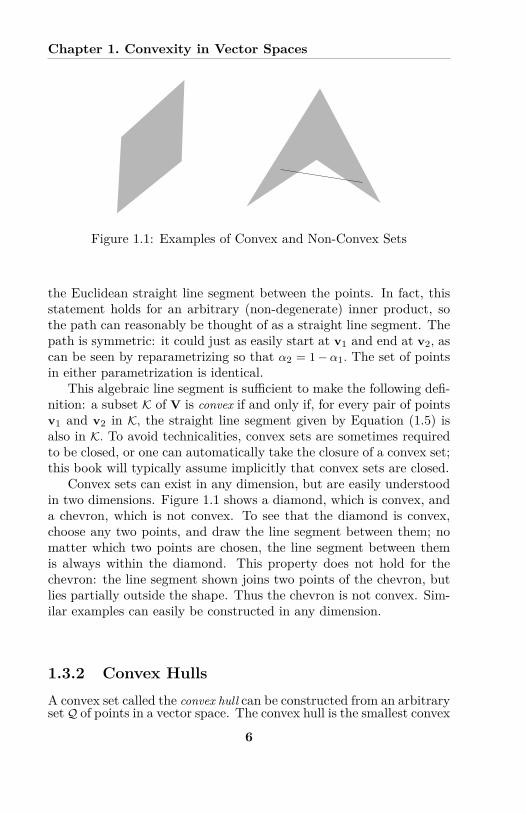
Figure 1.1: Examples of Convex and Non-Convex Sets
the Euclidean straight line segment between the points. In fact, thisstatement holds for an arbitrary (non-degenerate) inner product, sothe path can reasonably be thought of as a straight line segment. Thepath is symmetric: it could just as easily start at v1 and end at v2, ascan be seen by reparametrizing so that –2 = 1 ≠ –1. The set of pointsin either parametrization is identical.
This algebraic line segment is su�cient to make the following defi-nition: a subset K of V is convex if and only if, for every pair of pointsv1 and v2 in K, the straight line segment given by Equation (1.5) isalso in K. To avoid technicalities, convex sets are sometimes requiredto be closed, or one can automatically take the closure of a convex set;this book will typically assume implicitly that convex sets are closed.
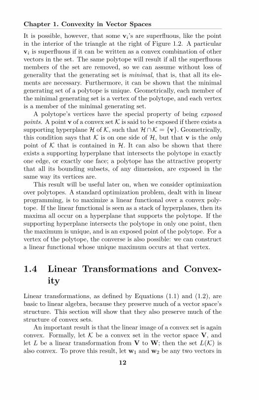
Convex sets can exist in any dimension, but are easily understoodin two dimensions. Figure 1.1 shows a diamond, which is convex, anda chevron, which is not convex. To see that the diamond is convex,choose any two points, and draw the line segment between them; nomatter which two points are chosen, the line segment between themis always within the diamond. This property does not hold for thechevron: the line segment shown joins two points of the chevron, butlies partially outside the shape. Thus the chevron is not convex. Sim-ilar examples can easily be constructed in any dimension.
1.3.2 Convex HullsA convex set called the convex hull can be constructed from an arbitraryset Q of points in a vector space. The convex hull is the smallest convex
6
1.3. Convex Sets in Vector Spaces
set that contains all the points in Q. As a set, it is given by
hull(Q) =
; mÿ
i=1
–ivi
----vi œ Q ’i, 0 Æ –i Æ 1 ’i, andmÿ
i=1
–i = 1<
, (1.7)
where m is any finite number. Note that Equation (1.7) is just Equa-tion (1.5), with 2 replaced by m. In general, a convex combination of m
vectors is a linear combination of those vectors, with the requirementsthat each coe�cient in the combination is between 0 and 1 inclusive,and that the coe�cients sum to 1. Equation (1.7) then says that theconvex hull of Q consist of all convex combinations of all finite subsetsof Q. If Q consists of three (non-collinear) vectors, then their convexhull is just the triangle for which those vectors are vertices. Similarly,the diamond in Figure 1.1 is the convex hull of its four vertices.
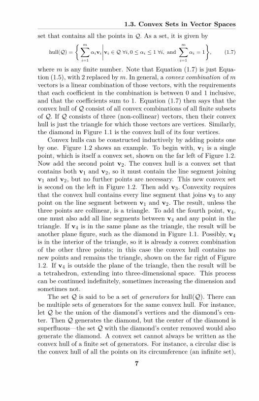
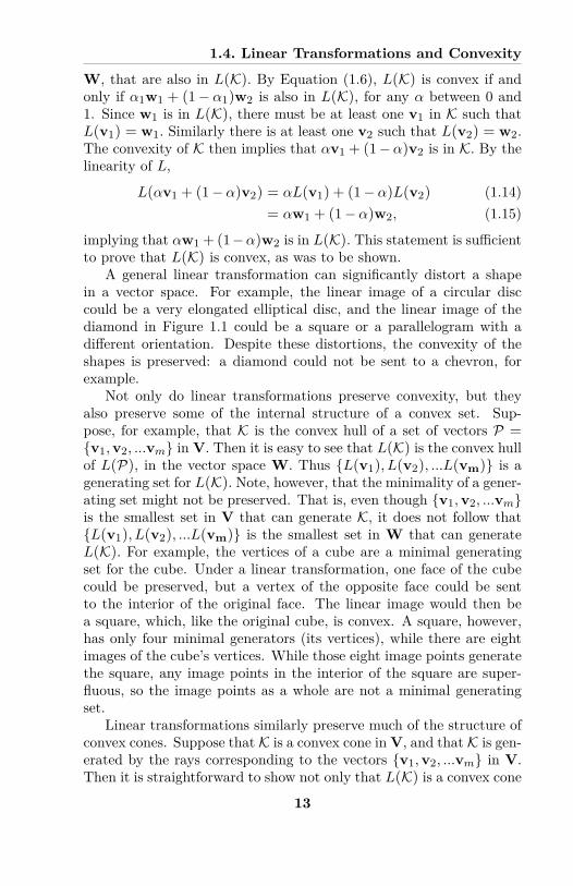
Convex hulls can be constructed inductively by adding points oneby one. Figure 1.2 shows an example. To begin with, v1 is a singlepoint, which is itself a convex set, shown on the far left of Figure 1.2.Now add the second point v2. The convex hull is a convex set thatcontains both v1 and v2, so it must contain the line segment joiningv1 and v2, but no further points are necessary. This new convex setis second on the left in Figure 1.2. Then add v3. Convexity requiresthat the convex hull contains every line segment that joins v3 to anypoint on the line segment between v1 and v2. The result, unless thethree points are collinear, is a triangle. To add the fourth point, v4,one must also add all line segments between v4 and any point in thetriangle. If v4 is in the same plane as the triangle, the result will beanother plane figure, such as the diamond in Figure 1.1. Possibly, v4is in the interior of the triangle, so it is already a convex combinationof the other three points; in this case the convex hull contains nonew points and remains the triangle, shown on the far right of Figure1.2. If v4 is outside the plane of the triangle, then the result will bea tetrahedron, extending into three-dimensional space. This processcan be continued indefinitely, sometimes increasing the dimension andsometimes not.
The set Q is said to be a set of generators for hull(Q). There canbe multiple sets of generators for the same convex hull. For instance,let Q be the union of the diamond’s vertices and the diamond’s cen-ter. Then Q generates the diamond, but the center of the diamond issuperfluous—the set Q with the diamond’s center removed would alsogenerate the diamond. A convex set cannot always be written as theconvex hull of a finite set of generators. For instance, a circular disc isthe convex hull of all the points on its circumference (an infinite set),
7
Chapter 1. Convexity in Vector Spaces
Figure 1.2: Constructing a Convex Hull Inductively
but not the convex hull of any smaller set of points.
1.3.3 Convex ConesAn important kind of convex set in a vector space is a ray. A ray is astraight line that starts at the origin, and continues on indefinitely insome direction. Formally, let v be a vector in V. Then the set
ray(v) = {–v|0 Æ –} (1.8)
defines the ray in the direction v. Informally speaking, a ray is halfof the one-dimensional subspace generated by v; any one-dimensionalsubspace is a straight line that goes through the origin and continues toinfinity in two opposite directions. The choice of v in Equation (1.8)is not unique: any positive multiple of v would generate the sameset. Like convex sets, rays can exist in a vector space of arbitrarydimension.
A convex cone is the convex hull of a set of rays (or, to be tech-nically correct, it is the convex hull of the union of all the pointscontained in all those rays). The set of rays is said to generate itsconvex cone. Without loss of generality, we can also define the convexcone of an arbitrary set of points Q as the convex cone of the raysresulting from each vector in Q. Formally, define
cone(Q) =
Imÿ
i=1–ivi
-----vi œ Q, 0 Æ –i
J, (1.9)
where m is any finite number. Equation (1.9) can easily be modified toapply to a set of rays: just define a set Q such that each ray is gener-ated by one vector in Q. It is easy to see that the same convex set will
8
1.3. Convex Sets in Vector Spaces
Supporting HyperplaneOrigin
Origin
Figure 1.3: Proper and Improper Convex Cones
result, regardless of the choice of the rays’ generating vectors. Thelinear combinations in Equation (1.9) might be called non-negativecombinations, because their coe�cients are all non-negative—but oth-erwise arbitrary, as opposed to convex combinations, which require inaddition that all coe�cients sum to 1.
Suppose there are two rays. Then their convex cone is the infinitewedge between them. Note that this wedge is in the smaller of the twoangles between the rays. In the special case in which the two rays are inopposite directions, their convex cone collapses to a single line throughthe origin. If the two rays are in a vector space of dimension greaterthan two, then the convex cone is restricted to the two-dimensionalplane that the rays span.
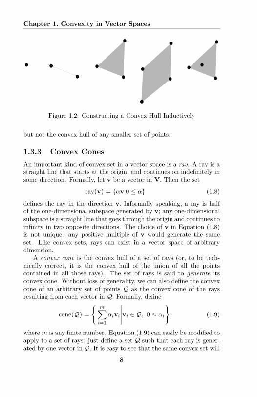
If a third ray is added, then the convex cone is usually a triangularpyramid whose apex is the origin and whose “base” is infinitely faraway. An instructive example occurs when the three rays are in atwo-dimensional vector space. Figure 1.3 breaks this instance into theproper and improper cases, which give qualitatively di�erent results.In this figure, the solid black lines represent rays through the origin,and the grey regions are the convex cones. At the left of the figure,all three rays are on the same side of a line through the origin; thenthe convex cone is again a wedge, with one of the rays inside it. Theoutside line is a hyperplane, which separates the convex cone fromthe rest of the vector space; such a hyperplane is called a supportinghyperplane. This hyperplane is not unique; many choices could bemade for it.
In the second case, no such separating line exists; then the convex
9
Chapter 1. Convexity in Vector Spaces
cone is the entire plane. The dividing line between the two casesoccurs when the total angle of the cone at the origin is 180¶. In thecase on the left, the bounding rays could be spread apart until theangle between them reaches 180¶. A supporting hyperplane would stillexist, and the convex cone would contain at most a half-space. Oncethe angle exceeds 180¶, however, the convex cone contains the entirevector space. There are no intermediate cases. There could not be,for example, a convex cone of angle 240¶. In higher dimensions, theseparating line becomes a supporting hyperplane, and the cone canhave higher dimension than two. All the same considerations applywhen there are more than three rays: a supporting hyperplane can beeither found or not, no matter how many rays are in the set.
The cone on the left is called a proper cone, because it fits ourintuitive idea of what a cone should be better than the cone on theright. Formally, a cone is said to be proper if it does not contain anyone-dimensional subspaces; geometrically, of course, one-dimensionalsubspaces are just straight lines through the origin. Equivalently, if aproper cone contains a non-zero vector v, then it cannot also contain≠v. This condition allows the construction of a functional which isalways non-negative, whose kernel is a supporting hyperplane throughthe origin. An improper cone contains both v and ≠v for some vec-tor, so any (non-zero) functional on an improper cone takes on bothpositive and negative values.
An important case of a proper convex cone in a vector space Vis a non-negative octant, denoted O. Non-negative octants are notunique—there are di�erent ones for di�erent choices of basis. Once aparticular basis is fixed, O consists of the convex cone generated by thebasis rays, where a basis ray is a ray in the direction of a basis vector.Equivalently, O contains any vector whose coordinates, when writtenin the fixed basis, are all non-negative. The convexity of O is evident,because a convex combination of any two non-negative vectors is againa non-negative vector, as can be seen from Equation (1.5).
A simple example is the vector space R3, in Cartesian coordinates.The non-negative octant is then a “cube” that extends to infinity. Ithas three infinite edges, which are the basis rays in the x, y, and z
directions. The co-ordinate vectors for these rays are (1, 0, 0), (0, 1, 0),and (0, 0, 1). Clearly every non-negative vector can be written as anon-negative linear combination of these three vectors, and every non-negative linear combination gives a non-negative vector, showing thatthe non-negative octant is identical with the convex cone of the basisrays. This example easily generalizes to higher dimensions.
10
1.3. Convex Sets in Vector Spaces
It is easy to see geometrically that there exists a supporting hyper-plane, in fact many supporting hyperplanes, for O, satisfying the firstcase in Figure 1.3. One such hyperplane, H, is the kernel of the linearfunctional F , given by
F (v) =nÿ
i=1vi, (1.10)
where the vi’s are the coordinates of v in terms of a fixed basis, givenby vectors {b1, b2, ...bn} :
v =nÿ
i=1vibi. (1.11)
In R3 with Cartesian coordinates, this functional would be written asF (x, y, z) = x + y + z.
The hyperplane H is the kernel of F , given by
H = ker F = {v œ V |F (v) = 0}. (1.12)
Since F applied to any non-negative vector (except the origin) isgreater than 0, and since F is 0 on any vector in H, it follows fromthe previous discussion that all of O is on one side of H (exceptingthe origin itself, which is contained in H). H is therefore a supportinghyperplane that separates the non-negative octant from a half-spaceof V.
1.3.4 Convex PolytopesA particularly simple and important kind of convex set is called aconvex polytope, which is defined to be the convex hull of a finite setof points. A polytope can be thought of as an n-dimensional gener-alization of polygons and polyhedra. A convex polyhedron consistsof a three-dimensional interior, bounded by two-dimensional polygo-nal faces; each bounding polygon is itself convex and is bounded byconvex line segments, which are themselves bounded by isolated ver-tices. Similarly, a general n-dimensional convex polytope is boundedby a set of (n ≠ 1)-dimensional convex polytopes, which are themselvesbounded by (n ≠ 2)-dimensional convex polytopes, and so on, until thevertices are reached.
Since a convex polytope P is the convex hull of a finite set, we canwrite
P = hull ({v1, v2, ..., vm}) . (1.13)
11
Chapter 1. Convexity in Vector Spaces
It is possible, however, that some vi’s are superfluous, like the pointin the interior of the triangle at the right of Figure 1.2. A particularvi is superfluous if it can be written as a convex combination of othervectors in the set. The same polytope will result if all the superfluousmembers of the set are removed, so we can assume without loss ofgenerality that the generating set is minimal, that is, that all its ele-ments are necessary. Furthermore, it can be shown that the minimalgenerating set of a polytope is unique. Geometrically, each member ofthe minimal generating set is a vertex of the polytope, and each vertexis a member of the minimal generating set.
A polytope’s vertices have the special property of being exposedpoints. A point v of a convex set K is said to be exposed if there exists asupporting hyperplane H of K, such that H fl K = {v}. Geometrically,this condition says that K is on one side of H, but that v is the onlypoint of K that is contained in H. It can also be shown that thereexists a supporting hyperplane that intersects the polytope in exactlyone edge, or exactly one face; a polytope has the attractive propertythat all its bounding subsets, of any dimension, are exposed in thesame way its vertices are.
This result will be useful later on, when we consider optimizationover polytopes. A standard optimization problem, dealt with in linearprogramming, is to maximize a linear functional over a convex poly-tope. If the linear functional is seen as a stack of hyperplanes, then itsmaxima all occur on a hyperplane that supports the polytope. If thesupporting hyperplane intersects the polytope in only one point, thenthe maximum is unique, and is an exposed point of the polytope. For avertex of the polytope, the converse is also possible: we can constructa linear functional whose unique maximum occurs at that vertex.
1.4 Linear Transformations and Convex-ity
Linear transformations, as defined by Equations (1.1) and (1.2), arebasic to linear algebra, because they preserve much of a vector space’sstructure. This section will show that they also preserve much of thestructure of convex sets.
An important result is that the linear image of a convex set is againconvex. Formally, let K be a convex set in the vector space V, andlet L be a linear transformation from V to W; then the set L(K) isalso convex. To prove this result, let w1 and w2 be any two vectors in
12
1.4. Linear Transformations and Convexity
W, that are also in L(K). By Equation (1.6), L(K) is convex if andonly if –1w1 + (1 ≠ –1)w2 is also in L(K), for any – between 0 and1. Since w1 is in L(K), there must be at least one v1 in K such thatL(v1) = w1. Similarly there is at least one v2 such that L(v2) = w2.The convexity of K then implies that –v1 + (1 ≠ –)v2 is in K. By thelinearity of L,
L(–v1 + (1 ≠ –)v2) = –L(v1) + (1 ≠ –)L(v2) (1.14)= –w1 + (1 ≠ –)w2, (1.15)
implying that –w1 + (1 ≠ –)w2 is in L(K). This statement is su�cientto prove that L(K) is convex, as was to be shown.
A general linear transformation can significantly distort a shapein a vector space. For example, the linear image of a circular disccould be a very elongated elliptical disc, and the linear image of thediamond in Figure 1.1 could be a square or a parallelogram with adi�erent orientation. Despite these distortions, the convexity of theshapes is preserved: a diamond could not be sent to a chevron, forexample.
Not only do linear transformations preserve convexity, but theyalso preserve some of the internal structure of a convex set. Sup-pose, for example, that K is the convex hull of a set of vectors P ={v1, v2, ...vm} in V. Then it is easy to see that L(K) is the convex hullof L(P), in the vector space W. Thus {L(v1), L(v2), ...L(vm)} is agenerating set for L(K). Note, however, that the minimality of a gener-ating set might not be preserved. That is, even though {v1, v2, ...vm}is the smallest set in V that can generate K, it does not follow that{L(v1), L(v2), ...L(vm)} is the smallest set in W that can generateL(K). For example, the vertices of a cube are a minimal generatingset for the cube. Under a linear transformation, one face of the cubecould be preserved, but a vertex of the opposite face could be sentto the interior of the original face. The linear image would then bea square, which, like the original cube, is convex. A square, however,has only four minimal generators (its vertices), while there are eightimages of the cube’s vertices. While those eight image points generatethe square, any image points in the interior of the square are super-fluous, so the image points as a whole are not a minimal generatingset.
Linear transformations similarly preserve much of the structure ofconvex cones. Suppose that K is a convex cone in V, and that K is gen-erated by the rays corresponding to the vectors {v1, v2, ...vm} in V.Then it is straightforward to show not only that L(K) is a convex cone
13
Chapter 1. Convexity in Vector Spaces
in W, but also that the rays generated by {L(v1), L(v2), ...L(vm)}are a generating set for the new convex cone. Again, some of thoseimage rays might be superfluous, if L sends one of the vi’s to the in-terior of the new cone. The fact that linear transformations preserveconvex cones will be directly relevant to colour investigations in Chap-ter 4, when we investigate a transformation from the vector space ofradiometric functions to the vector space of perceived colours.
1.5 Euclidean NotionsAlthough this book emphasizes geometric naturalness in its presenta-tion, some very natural Euclidean notions, such as distance and angle,do not appear, and in fact are not needed. Somewhat surprisingly, thecombinatorial structure—the fact that certain vectors sum to certainother vectors—and the linear relationships between vector spaces con-tain all the information needed for developing colour matching math-ematically. A general vector space, in fact, has no notion of length orangle, unless one imposes some additional properties, such as an innerproduct. The reader should be warned against using the standard dotproduct to define magnitudes or perpendicular projections, or to in-terpret conclusions in those terms: the dot product implicitly assumesthat an orthonormal basis exists, while the vector spaces used in thisbook provide no concepts of right angle or unit length.
1.6 Chapter SummaryThis chapter has introduced the concept of convexity, in a vector spacesetting. The following standard definitions and results of linear algebrawere used:
1. A linear functional F is a linear transformation from a vectorspace V to the real numbers R,
2. A hyperplane H (or more properly, an a�ne hyperplane) in avector space V of dimension n is an (n ≠ 1)-dimensional vectorsubspace, that has been translated by the addition of an arbi-trary vector v,
3. Let – be a real number, and let F be a non-degenerate functional(i.e. F takes on some non-zero values) on V . Then the pre-imageF
≠1(–) is a hyperplane H in V ,
14
1.6. Chapter Summary
4. Suppose F is a non-degenerate functional on V . Then the setof all hyperplanes, that are pre-images under F of an arbitraryreal number –, foliate V : each vector v in V belongs to exactlyone hyperplane. The hyperplanes can be indexed by assigningthe value F (H) to each hyperplane H in the foliation. Underthis indexing, the hyperplane F
≠1(0) contains the origin, andthe hyperplanes with positive indices are stacked linearly, in theorder given by their indices, away from the origin; a symmetricalresult holds for hyperplanes with negative indices,
5. If two functionals produce the same hyperplane foliation, thenthe two functionals are scalar multiples of each other.
A vector space V contains su�cient structure to define and con-struct convex sets. The following standard definitions and results wereintroduced:
1. Given two vectors v1 and v2 in V, the line segment betweenthem is the set defined by
{–1v1 + (1 ≠ –1)v2|0 Æ –1 Æ 1}. (1.16)
Using – as an index parametrizes the line segment continuously,as an image of the real interval [0, 1],
2. A subset K of V is convex if, for every v1 and v2 in K, the linesegment between v1 and v2 is contained in K,
3. Let Q be a set of points in V . Then the convex hull of Q, denotedhull(Q), is the smallest convex set that contains every point inQ. As a set, hull(Q) is given by
hull(Q) =
; mÿ
i=1
–ivi
----vi œ Q ’i, 0 Æ –i Æ 1 ’i andmÿ
i=1
–i = 1<
. (1.17)
Algebraically, hull(Q) is the set of convex combinations of arbi-trary finite subsets of Q, where a convex combination of vectorsis a linear combination of those vectors, whose coe�cients arebetween 0 and 1 inclusive, and which sum to 1,
4. Let Q be a set of points in V . Then the convex cone of Q, denotedcone(Q), is the set
cone(Q) =
Imÿ
i=1–ivi
-----, vi œ Q, 0 Æ –i
J, (1.18)
5. A convex polytope (sometimes called just a polytope) is the con-vex hull of a finite set of points,
15
Chapter 1. Convexity in Vector Spaces
6. Geometrically, a convex polytope can be written as the convexhull of its vertices, which are a unique subset of the polytope.
7. Each vertex v of a convex polytope P is an exposed point, thatis: there exists a hyperplane H such that H contains v, but Hcontains no other point of P.
Linear transformations a�ect convex subsets of an underlying vec-tor space as follows:
1. Linear transformations preserve convexity. Suppose a lineartransformation L goes from a vector space V to a vector spaceW, and that K is a convex set in V. Then L(K) is a convex setin W.
2. Furthermore, if Q is a set of points in V, then a linear trans-formation L preserves some of the internal structure of convexsets:
L(hull(Q)) = hull(L(Q)), and (1.19)L(cone(Q)) = cone(L(Q)). (1.20)
Finally, the reader should keep in mind that a general vector space,and in particular the vector spaces treated in this book, have no con-cept of distance or angle, so the book’s conclusions should not beunderstood in Euclidean terms. Instead, combinatorial and linear re-lationships provide all the structure needed.
16
Chapter 2
Zonohedra
2.1 IntroductionA zonohedron Z is a special kind of convex polytope, that consistsof all the linear combinations of a set of vectors in R3, provided thatthe coe�cients in each combination are between 0 and 1 inclusive.The set of such combinations is a special instance of the Minkowskisum, sometimes also called the vector sum. Zonohedra occur in colourscience when simple colours, such as the primaries of an electronic dis-play or single-wavelength radiometric functions, combine to producenew colours. Each simple colour can be represented as a vector inthree-dimensional perceptual colour space. The vector for a colourcombination is a linear combination of vectors for the simple colours,with the physical restriction that the coe�cients in the combinationcannot exceed 1. The set of all possible colour mixtures is thus a zono-hedron. This chapter derives some geometric properties of zonohedra.Later chapters will use the geometric properties to derive further re-sults about colour.
The Minkowski sum of two subsets of a vector space is a newsubset, consisting of all sums of pairs of vectors, where the first vectorbelongs to the first subset and the second vector belongs to the secondsubset. This definition can easily be extended to include an arbitrarynumber of subsets, rather than just two, and the order of the subsetsis immaterial. Typically, the Minkowski sum is applied to convexsubsets, in which case it produces another convex subset. Apart fromits simple algebraic definition, the Minkowski sum also has a concretegeometric interpretation: the Minkowski sum of two subsets is, up to
17
Chapter 2. Zonohedra
a translation, the set produced by placing a copy of the first subsetover every point of the second subset. More dynamically, one subsetis “swept” over the entirety of the other subset, and any point that iscovered by the sweeping action is contained in the Minkowski sum.
Geometrically, a vector can be interpreted as either an isolatedpoint in a vector space, or as the line segment that joins that pointto the origin. The Minkowski sum can be applied to a set of vec-tors, called generating vectors, by interpreting those vectors as linesegments, which are convex subsets of the overall space. In three di-mensions, the Minkowski sum of a set of vectors is called a zonohedron.
The Minkowski sum of two vectors is the filled parallelogram thatis swept out when one vector slides over the other. Visually, one canpicture the first vector moving continuously as its tail slides along theline segment corresponding to the second vector. Then sweep a thirdvector, that is not coplanar with the first two, over the parallelogram,producing a solid parallelepiped. This solid is the Minkowski sum ofall three vectors, and is a zonohedron. In R3, a fourth vector could beMinkowski-summed with the parallelepiped, producing a new, morecomplicated, zonohedron, and in fact any number of vectors could besimilarly Minkowki-summed to produce a zonohedron.
Zonohedra have many useful properties. For instance, a zonohe-dron’s faces are parallelograms, and its edges are translated copies ofthe generating vectors. Each vertex can be written uniquely as the sumof all the generating vectors that lie on one side of a plane through theorigin. A zonohedron is encircled by bands called zones, where eachzone corresponds to a generating vector. Furthermore, a zonohedronis centrally symmetric. This chapter constructs Minkowski sums andzonohedra intuitively, and derives such properties. While zonohedrageneralize naturally to zonotopes in arbitrary dimensions, we will re-strict ourselves to R3, which is su�cient for colour matching. Whileno results in this chapter are new, their systematic and concrete pre-sentation from first principles is believed to be the only one availableso far.
2.2 The Minkowski Sum2.2.1 Definition and PropertiesIn visual terms, the Minkowski sum, sometimes also called the vectorsum, can be pictured as a way of adding shapes or solids, or, indeed,arbitrary subsets of a vector space. It is a simple, intuitive construc-
18
2.2. The Minkowski Sum
tion, both algebraically and geometrically. Formally, let A and B betwo non-empty subsets of a vector space Rn. Then their Minkowskisum, denoted ü, is defined as
A ü B =)
vA + vB--vA œ A and vB œ B
*. (2.1)
In this equation, vA and vB are both vectors in Rn, and the plus signon the right-hand side indicates vector addition.
The commutativity of the vector addition in Equation (2.1) impliesthat the Minkowski sum is commutative, so A ü B = B ü A. Further-more, the associativity of vector addition implies that (A ü B) ü C =A ü (B ü C), if there were a third subset C. Together, commutativ-ity and associativity imply that the Minkowski sum of any number ofsummands is well-defined, regardless of the order of those summands.
Although the Minkowski sum is defined for arbitrary subsets A andB, it is most commonly applied to convex subsets, which will be thecase of interest for this book. When A and B are both convex, thenA ü B is also convex. To demonstrate this statement, let v and w betwo vectors in A ü B, and let – be a scalar between 0 and 1; convexitywill follow if we can show that –v+ (1 ≠ –)w œ A ü B. Since v and ware both in the Minkowski sum of A and B, there must exist vectorssuch that
v = vA + vB, (2.2)w = wA + wB, (2.3)
where the subscripts indicate which subsets the vectors belong to.Since A and B are both convex, it follows that
–vA + (1 ≠ –)wA œ A, (2.4)–vB + (1 ≠ –)wB œ B. (2.5)
Equation (2.4) gives a vector in A, and Equation (2.5) gives a vectorin B, so their sum is in A ü B :
–(vA + vB) + (1 ≠ –)(wA + wB) œ A ü B. (2.6)
Substituting Equations (2.2) and (2.3) into Equation (2.6) gives
–v + (1 ≠ –)w œ A ü B, (2.7)
implying that A ü B is convex, as was to be shown.
19
Chapter 2. Zonohedra
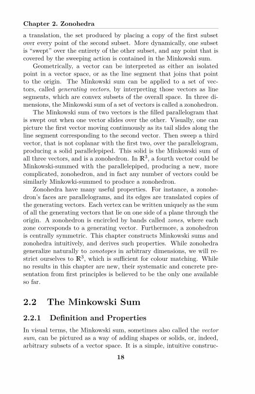
2.2.2 Some Two-Dimensional ExamplesThough Minkowski sums are defined in arbitrary dimensions, somesimple two-dimensional examples provide geometric motivation. Forthe first example, let A be a triangle in the positive quadrant of R2,and let B be a small disc centered on the origin, as shown in the leftof Figure 2.1. Let vA be a point in the triangle. It follows easily fromthe definition that A ü B is the union of all the sets vA + B, over allpoints vA in A. The set vA +B is a small disc that is centered on vA.This disc is a translation of the set B, and is contained in A ü B.
A
B
A+B
Figure 2.1: An Example of a Minkowski Sum
If vA is well in the interior of A, then vA + B is contained com-pletely in A. If vA is on the perimeter of A, however, then vA + Bextends somewhat outside A. The middle of Figure 2.1 shows the trans-lated discs along the triangle’s edges; these discs are included in theMinkowski sum. One can picture the disc sliding along each edge, andsweeping out a band on either side of the edge; the band on the tri-angle’s exterior produces a parallel contour that expands the triangle.Once the disc reaches a vertex, the band changes direction abruptly,and its contour is now an arc of the disc rather than a straight line.
The Minkowski sum is the union of the triangle’s interior, the bandsalong the three edges, and the circular sectors at the three vertices, asshown on the right in Figure 2.1. A unifying interpretation is that theMinkowski sum consists of all the points the disc would cover, if it wereswept over every point on the triangle. Note that the sweeping is doneby fixing a point on the disc, in this case its center, and letting thatcenter sweep over the triangle. The origin was chosen as a convenientlocation for this example because, when the center is at the origin,adding it to A does not move A.
20
2.2. The Minkowski Sum
Arc of Circle
Arc of Circle
Arc of Circle
Edge of Triangle
Edge of
Triangle
Edge of Triangle
Perimeter ofMinkowski Sum
Segments of Summands' Perimeters
Figure 2.2: The Perimeter of a Minkowski Sum
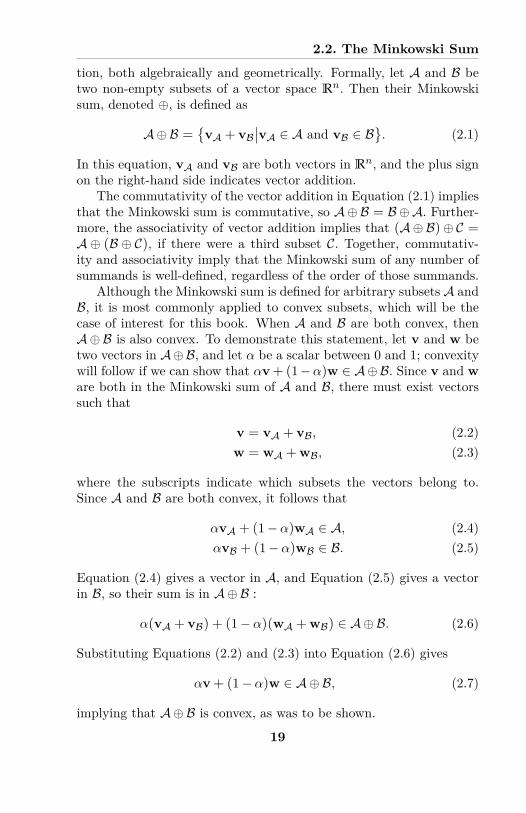
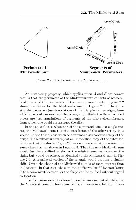
An interesting property, which applies when A and B are convexsets, is that the perimeter of the Minkowski sum consists of reassem-bled pieces of the perimeters of the two summand sets. Figure 2.2shows the pieces for the Minkowski sum in Figure 2.1. The threestraight pieces are just translations of the triangle’s three edges, fromwhich one could reconstruct the triangle. Similarly the three roundedpieces are just translations of segments of the disc’s circumference,from which one could reconstruct the disc.
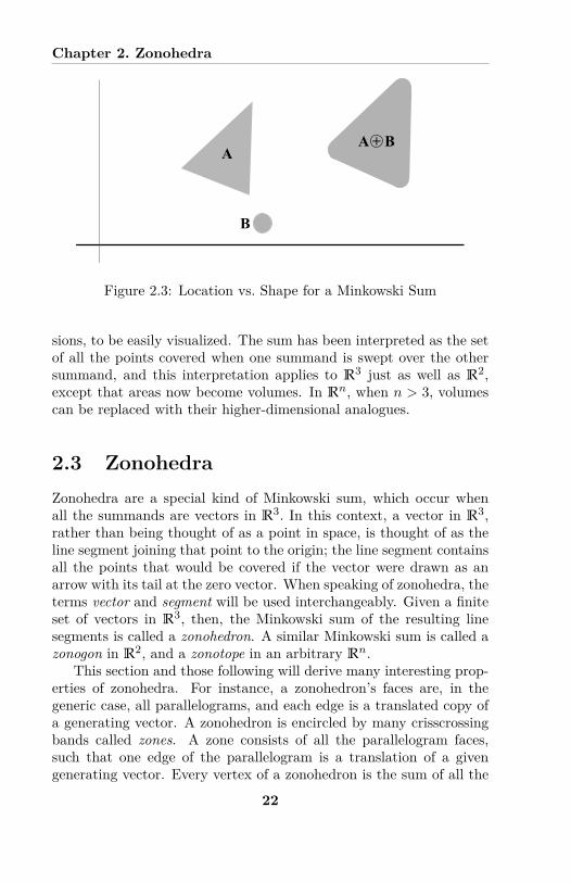
In the special case when one of the summand sets is a single vec-tor, the Minkowski sum is just a translation of the other set by thatvector. In the trivial case when one summand set consists solely of theorigin, the Minkowski sum is just an unmodified copy of the other set.Suppose that the disc in Figure 2.1 was not centered at the origin, butsomewhere else, as shown in Figure 2.3. Then the new Minkowki sumwould just be a shifted version of the original sum, as shown on theright, but would be otherwise identical to the Minkowski sum in Fig-ure 2.1. A translated version of the triangle would produce a similarshift. Often the shape of the Minkowski sum is of more interest thanits location. In that case, the sum can be “normalized” by translatingit to a convenient location, or the shape can be studied without regardto location.
The discussion so far has been in two dimensions, but should allowthe Minkowski sum in three dimensions, and even in arbitrary dimen-
21
Chapter 2. Zonohedra
A
B
A + B
Figure 2.3: Location vs. Shape for a Minkowski Sum
sions, to be easily visualized. The sum has been interpreted as the setof all the points covered when one summand is swept over the othersummand, and this interpretation applies to R3 just as well as R2,except that areas now become volumes. In Rn, when n > 3, volumescan be replaced with their higher-dimensional analogues.
2.3 ZonohedraZonohedra are a special kind of Minkowski sum, which occur whenall the summands are vectors in R3. In this context, a vector in R3,rather than being thought of as a point in space, is thought of as theline segment joining that point to the origin; the line segment containsall the points that would be covered if the vector were drawn as anarrow with its tail at the zero vector. When speaking of zonohedra, theterms vector and segment will be used interchangeably. Given a finiteset of vectors in R3, then, the Minkowski sum of the resulting linesegments is called a zonohedron. A similar Minkowski sum is called azonogon in R2, and a zonotope in an arbitrary Rn.
This section and those following will derive many interesting prop-erties of zonohedra. For instance, a zonohedron’s faces are, in thegeneric case, all parallelograms, and each edge is a translated copy ofa generating vector. A zonohedron is encircled by many crisscrossingbands called zones. A zone consists of all the parallelogram faces,such that one edge of the parallelogram is a translation of a givengenerating vector. Every vertex of a zonohedron is the sum of all the
22
2.3. Zonohedra
generating vectors that are on one side of a plane through the origin.Furthermore, a zonohedron is centrally symmetric: its shape at theorigin and its shape at the farthest vertex are reversed, but otherwiseidentical. Cyclic zonohedra are a useful subclass, whose zones take aconvenient form; cyclic zonohedra arise when the generating vectorsare all on the boundary of a convex cone.
Zonotopes occur naturally when a number of ingredients, in a gen-eral sense, are combined, again in a general sense, to make a new mix-ture, and the maximum quantity of each ingredient is limited. Eachingredient can be represented by a vector whose head represents themaximum possible quantity of that ingredient while the tail, at theorigin, means that none of that ingredient is used. The set of all pos-sible mixtures is the Minkowski sum of the ingredients’ vectors, and isthus a zonotope.
Later in this book, surface colours and other objects of interestwill be expressed as just such mixtures. At each wavelength, a sur-face colour reflects between 0 and 100 percent of the incoming light.The colour corresponding to each wavelength is a vector in a three-dimensional perceptual space. The contribution at each wavelengthis an “ingredient” in the overall colour, which is the “mixture” of thereflected light at each wavelength. The set of all surface colours, whenviewed in a certain illumination, is called an object-colour solid, andthis interpretation implies that it is a zonohedron. By similar construc-tions, an electronic display gamut, which is the set of all the coloursthat that display can produce, is also a zonohedron. The zonohedralform of these objects of colour science is the central insight of thisbook. Later chapters will use the formalism of this chapter to con-struct colour zonohedra, and then derive results in colour science fromzonohedral properties.
2.3.1 DefinitionsSuppose we denote a set of m vectors, or equivalently m line segmentsstarting at the origin, in Rn, by
G = {v1, v2, ..., vm}. (2.8)
Then the zonotope Z generated by G is defined to be the Minkowskisum of those segments:
Z(G) = v1 ü v2 ü ... ü vm. (2.9)
23
Chapter 2. Zonohedra
G is referred to as the set of generating vectors, or just generators, forZ. When n = 2, Rn is the plane, and Z is called a zonogon. Whenn = 3, Rn is three-dimensional space, and Z is called a zonohedron.
Since the line segment corresponding to a vector v is given by theset
{–v|0 Æ – Æ 1}, (2.10)
it follows that an equivalent definition for a zonotope is
Z(G) =I
mÿ
i=1–ivi
-----0 Æ –i Æ 1 ’i
J. (2.11)
This definition of a zonotope is similar to the definition of a convexhull given by Equation 1.7, except that the coe�cients in a convexhull must sum to 1, while zonotope coe�cients lack that restriction,although they must still be between 0 and 1. Such a linear combina-tion, where all the coe�cients are between 0 and 1 inclusive, is called azonal combination. Equation (2.11) makes calculations easier, becausethe –i’s provide a convenient coordinatization. For geometric under-standing, however, Equation (2.9) is preferred, because it indicateshow a zonotope is constructed.
While the set of vectors G is arbitrary, this book will simplify cal-culations by further assuming that each vector in G is in the non-negative octant O relative to some basis. Then all the coordinates ofthe vi’s are non-negative, and the zonotope as a whole is containedin the non-negative octant. Such a zonotope is referred to as a non-negative zonotope. Non-negative zonotopes or zonohedra are adequatefor colour science, whose geometric objects are non-negative by con-struction. This approach avoids technical complications, such as twogenerating vectors that are in exactly opposite directions.
One immediate conclusion, using the results of Section 2.2.1, isthat a zonotope is always convex, since it is the Minkowski sum ofline segments, which are themselves convex. Zonotopes, and in par-ticular zonohedra, have considerably more structure, however, whichthis chapter will elucidate, after investigating some examples. Thefirst examples will be some simple zonogons in R2, which will then begeneralized to zonohedra in R3.
24
2.4. Construction of Zonogons
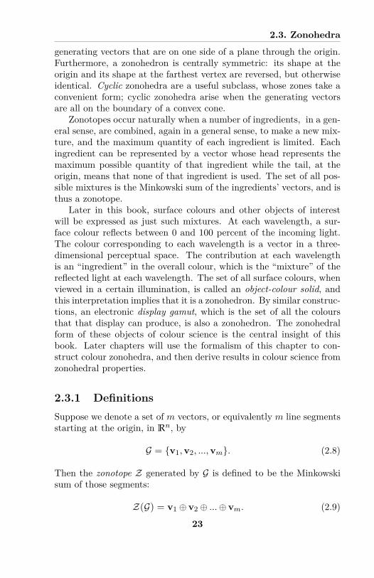
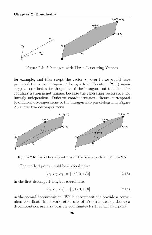
2.4 Construction of ZonogonsA zonogon is a two-dimensional zonotope. For a simple example, startwith two vectors, v1 and v2, in the non-negative octant of R2, as shownon the left of Figure 2.4. The Minkowski sum of the two vectors, orof their corresponding segments, is the area swept out when the firstsegment is moved continuously, with its tail following the entire lengthof the second segment. The right side of Figure 2.4 shows the result:the zonogon is a parallelogram with one vertex at the origin.
v1+v2
v1
v2
0v1
v2
0Figure 2.4: A Zonogon with Two Generating Vectors
This construction is symmetric: if the second vector swept over thefirst, the same parallelogram would result. Algebraically, the symme-try results from the commutativity of the Minkowski sum. The con-struction also increases area: even though each segment has zero area,their Minkowski sum has positive area. In this simple case, Equation(2.11) indicates a coordinatization for the parallelogram: any point isa unique linear combination of v1 and v2, both of whose coe�cientsare between 0 and 1.
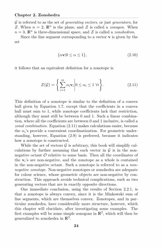
Now let us add a third vector, v3, as shown in the left of Figure2.5, and find the zonogon generated by all three vectors. Since theMinkowski sum is both commutative and associative, the order of itssummands is immaterial, and we can write
v1 ü v2 ü v3 = (v1 ü v2) ü v3. (2.12)
The Minkowski sum v1 ü v2 already appears as a parallelogram inFigure 2.4, so let v3 sweep over that parallelogram. The resultingzonogon is the irregular, filled hexagon on the right in Figure 2.5.
This zonogon construction is again symmetric, this time in threevectors instead of two.. Had we started with the parallelogram v1 ü v3,
25
Chapter 2. Zonohedrav1+ +v2 v3
v1
v2
v3
0v1
v2
0
v1+v3
+v2 v3
Figure 2.5: A Zonogon with Three Generating Vectors
for example, and then swept the vector v2 over it, we would haveproduced the same hexagon. The –i’s from Equation (2.11) againsuggest coordinates for the points of the hexagon, but this time thecoordinatization is not unique, because the generating vectors are notlinearly independent. Di�erent coordinatization schemes correspondto di�erent decompositions of the hexagon into parallelograms; Figure2.6 shows two decompositions.
v1+
v1+ +v2 v3
v1+v2
v1
v2
0
v1+v3
+v2 v3
v1+ +v2 v3
v3
v1
v2
0
v1+v3
+v2 v3
Figure 2.6: Two Decompositions of the Zonogon from Figure 2.5
The marked point would have coordinates
[–1, –2, –3] = [1/2, 0, 1/2] (2.13)
in the first decomposition, but coordinates
[–1, –2, –3] = [1, 1/3, 1/8] (2.14)
in the second decomposition. While decompositions provide a conve-nient coordinate framework, other sets of –’s, that are not tied to adecomposition, are also possible coordinates for the indicated point.
26
2.4. Construction of Zonogons
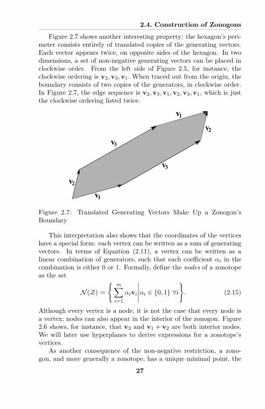
Figure 2.7 shows another interesting property: the hexagon’s peri-meter consists entirely of translated copies of the generating vectors.Each vector appears twice, on opposite sides of the hexagon. In twodimensions, a set of non-negative generating vectors can be placed inclockwise order. From the left side of Figure 2.5, for instance, theclockwise ordering is v2, v3, v1. When traced out from the origin, theboundary consists of two copies of the generators, in clockwise order.In Figure 2.7, the edge sequence is v2, v3, v1, v2, v3, v1, which is justthe clockwise ordering listed twice.
v1v2
v3
v1
v2
v3
Figure 2.7: Translated Generating Vectors Make Up a Zonogon’sBoundary
This interpretation also shows that the coordinates of the verticeshave a special form: each vertex can be written as a sum of generatingvectors. In terms of Equation (2.11), a vertex can be written as alinear combination of generators, such that each coe�cient –i in thecombination is either 0 or 1. Formally, define the nodes of a zonotopeas the set
N (Z) =
Imÿ
i=1–ivi
-----–i œ {0, 1} ’i
J. (2.15)
Although every vertex is a node, it is not the case that every node isa vertex; nodes can also appear in the interior of the zonogon. Figure2.6 shows, for instance, that v3 and v1 + v2 are both interior nodes.We will later use hyperplanes to derive expressions for a zonotope’svertices.
As another consequence of the non-negative restriction, a zono-gon, and more generally a zonotope, has a unique minimal point, the
27
Chapter 2. Zonohedra
origin, which occurs when every –i is 0, and a unique maximal, orterminal, point, which occurs when every –i is 1. Even though a gen-eral vector space implies no notion of distance, the terminal point is,loosely speaking, the “farthest” point from the origin. The center ofthe zonogon is halfway between the origin and the terminal point. Thezonogon is symmetric around the center: a 180¶ rotation about thecenter would map the zonogon to itself.
From the examples already given, adding further generating vectorsto produce new zonogons is straightforward: simply sweep the newvector over the zonogon for the previous vectors. The result will bea larger, more complicated, polygon that is still convex and centrallysymmetric, but whose boundary now includes two copies of the newvector.
2.5 Vectors in General PositionA special case occurs when one generator is a scalar multiple of anothergenerator. In this case, an edge of the zonogon consists of those twovectors laid end to end, and a node that is not a vertex appears onthe boundary. This configuration makes sense combinatorially, but isredundant geometrically, so we will use the concept of general positionto avoid it.
A set of vectors G in Rn is said to be in general position if everysubset of n vectors is linearly independent. Geometrically, a set of vec-tors in R2 is in general position if no two of them are scalar multiplesof each other, and vectors in R3 are in general position if no three ofthem are coplanar; analogues hold for higher dimensions. RequiringG to be in general position, or checking that an empirically found G isin general position, sidesteps many technical complications and allowsfor simpler descriptions. If generators in R2 are in general position,for instance, then each edge of a zonogon is a translated copy of asingle generator. Otherwise, an edge might consist of two generators,laid end to end. The property of being in general position is generic:an arbitrary set is most likely already in general position, and, if it isnot, a negligible adjustment will put the set in general position.
In the colour science applications to be studied, the generatingvectors are determined by empirical measurements, which are only ac-curate to some Á, so there is no information lost in adjusting any of themeasurements by an amount that is much smaller than Á. As a result,we can always obtain a set in general position, that agrees well with
28
2.6. Construction of Zonohedra
the measured data. Strictly speaking, any measurement uncertainty,no matter how small, makes it impossible to determine that two mea-sured vectors are scalar multiples of each other, or that three measuredvectors are coplanar; decisions about linear dependence therefore pro-ceed from theory or modeling. In fact, we will see a case in whicha set of vectors is nearly, but not quite, coplanar, and it will not beobvious whether the non-coplanarity is genuine, or an artifact of datasmoothing.
2.6 Construction of ZonohedraA zonohedron is constructed similarly to a zonogon, but in three di-mensions instead of two. Like the previous section, we will build anon-negative zonohedron generator by generator, letting interestingproperties emerge naturally.
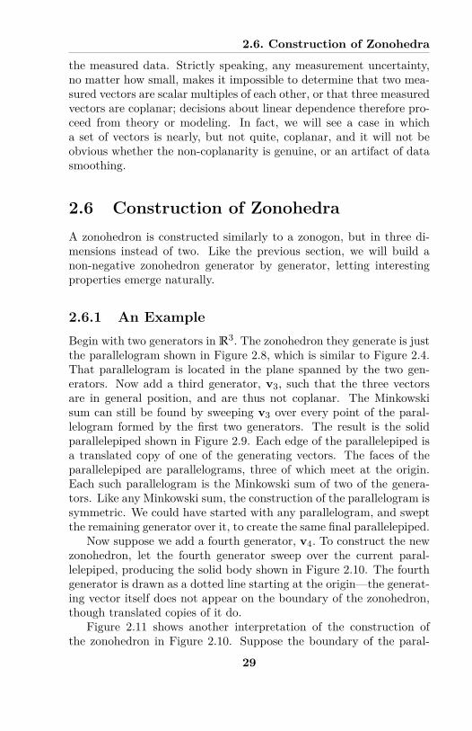
2.6.1 An ExampleBegin with two generators in R3. The zonohedron they generate is justthe parallelogram shown in Figure 2.8, which is similar to Figure 2.4.That parallelogram is located in the plane spanned by the two gen-erators. Now add a third generator, v3, such that the three vectorsare in general position, and are thus not coplanar. The Minkowskisum can still be found by sweeping v3 over every point of the paral-lelogram formed by the first two generators. The result is the solidparallelepiped shown in Figure 2.9. Each edge of the parallelepiped isa translated copy of one of the generating vectors. The faces of theparallelepiped are parallelograms, three of which meet at the origin.Each such parallelogram is the Minkowski sum of two of the genera-tors. Like any Minkowski sum, the construction of the parallelogram issymmetric. We could have started with any parallelogram, and sweptthe remaining generator over it, to create the same final parallelepiped.
Now suppose we add a fourth generator, v4. To construct the newzonohedron, let the fourth generator sweep over the current paral-lelepiped, producing the solid body shown in Figure 2.10. The fourthgenerator is drawn as a dotted line starting at the origin—the generat-ing vector itself does not appear on the boundary of the zonohedron,though translated copies of it do.
Figure 2.11 shows another interpretation of the construction ofthe zonohedron in Figure 2.10. Suppose the boundary of the paral-
29

Chapter 2. Zonohedra
v1v2
0
Figure 2.8: A Zonohedral Parallelogram
v1
v2
v3
0Figure 2.9: A Zonohedral Parallelepiped
v1
v2
v3
0
v4
v4
Figure 2.10: A Zonohedron with Four Generators
30
2.6. Construction of Zonohedra
v1
v2
v3
0
Figure 2.11: Another Construction of the Zonohedron in Figure 2.10
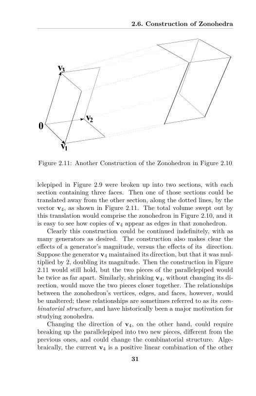
lelepiped in Figure 2.9 were broken up into two sections, with eachsection containing three faces. Then one of those sections could betranslated away from the other section, along the dotted lines, by thevector v4, as shown in Figure 2.11. The total volume swept out bythis translation would comprise the zonohedron in Figure 2.10, and itis easy to see how copies of v4 appear as edges in that zonohedron.
Clearly this construction could be continued indefinitely, with asmany generators as desired. The construction also makes clear thee�ects of a generator’s magnitude, versus the e�ects of its direction.Suppose the generator v4 maintained its direction, but that it was mul-tiplied by 2, doubling its magnitude. Then the construction in Figure2.11 would still hold, but the two pieces of the parallelepiped wouldbe twice as far apart. Similarly, shrinking v4, without changing its di-rection, would move the two pieces closer together. The relationshipsbetween the zonohedron’s vertices, edges, and faces, however, wouldbe unaltered; these relationships are sometimes referred to as its com-binatorial structure, and have historically been a major motivation forstudying zonohedra.
Changing the direction of v4, on the other hand, could requirebreaking up the parallelepiped into two new pieces, di�erent from theprevious ones, and could change the combinatorial structure. Alge-braically, the current v4 is a positive linear combination of the other
31
Chapter 2. Zonohedra
three generators, so it is “inside” the parallelepiped. The final zonohe-dron thus has three edges meeting at the origin. If v4 was not a positivelinear combination, then it would be “outside,” and four edges wouldmeet at the origin. These considerations will become important laterwhen discussing cyclic zonohedra.
2.6.2 Zonohedral Generators in General PositionRecall that a set of generating vectors in an n-dimensional vector spaceis in general position if every subset of n vectors is linearly indepen-dent. In three dimensions, the general position requirement avoidsthe case where one face of a zonohedron consists of three or more gen-erators; instead, each face is a parallelogram, each edge of which isa translated copy of a generator. Since a parallelogram’s four edgesbreak up into two pairs of parallel vectors, exactly two generators areneeded to specify each parallelogram face.
To see the relevance of general position, begin with the six-sidedzonogon shown in Figure 2.5. The three generators shown on theleft all lie in R2. Extend this zonogon to a zonohedron by adding afourth generator, which does not lie in the plane of the first threegenerators. Figure 2.12 shows the result, with the original zonogonin grey. The zonohedron is constructed by sweeping v4 over thatzonogon, resulting in a translated copy, that is also shown in grey. Thefirst three vectors are in general position in R2, because no two of themform a linearly dependent set. They are not in general position in R3,however, because the subset consisting of all three of them is linearlydependent. Geometrically, the lack of general position prevents thegrey face of the zonohedron from being a parallelogram.
The construction method shows that a zonohedron’s faces are allparallelograms if and only if the generators are in general position.Formally, we will present a demonstration that uses induction on thenumber of generators. Suppose that there are k generators, and thatthe zonohedron they generate only has parallelograms for faces. Nowadd a (k + 1)th generator, which does not form a linearly dependentset when combined with any two of the original generators. The newzonohedron is constructed, as in Figure 2.11, by breaking the originalzonohedron into two pieces (with breaks occurring only along edges,not on faces), translating one piece by vk+1, and introducing a new setof faces between the pieces. By the construction, each new face musthave two edges parallel to vk+1, and two edges that are parallel to oneof the original edges. Because of the assumption of general position,
32

2.6. Construction of Zonohedra
v3
v1
v2
0
v4
Figure 2.12: A Zonohedron when Generators are Not in General Po-sition
the new vector cannot be in the a�ne plane spanned by any pair of theoriginal vectors, so it cannot be in the plane of any of the zonohedron’soriginal faces. Thus all the new faces are in di�erent planes from allthe old faces. Since each new face has two pairs of parallel sides, eachnew face is a parallelogram, in a distinct plane from all previous faces.General position is thus su�cient to insure that all the faces of thenew zonohedron are parallelograms.
Conversely, suppose that the generators are not in general position,so that three generators are in the same plane. Since the order ofthe generators is irrelevant, start the construction of the zonohedronwith those three generators. They will generate a non-parallelogramface, such as appears in Figure 2.5. This face will be preserved (orperhaps be extended, if other vectors are also in that plane) as furthervectors are added, and so will appear in the final zonohedron. Generalposition is thus necessary if all the faces of the final zonohedron areparallelograms. The su�ciency and necessity together imply the “if
33
Chapter 2. Zonohedra
and only if” statement in the preceding paragraph, as was to be shown.Apart from introducing many di�culties in computations, non-
parallelogram faces are non-generic, in the sense discussed earlier, andcan often be eliminated. In particular, when the generating vectorsresult from a measurement process, their coordinates are always some-what uncertain, so no information is lost by adjusting one them by anamount that is orders of magnitude smaller than the measurementvariability. If three vectors are coplanar, then modifying one vectorvery slightly moves it out of the plane spanned by the other two.
In Figure 2.12, for example, v3 could be raised a tiny amount sothat it is no longer in the same plane as v1 and v2. Figure 2.13 showsthe result. The point v3 + v4 in Figure 2.13 is now slightly abovethe upper grey face, while in Figure 2.12 it was right on that face.The irregular hexagon has been decomposed into three parallelogramfaces, all in slightly di�erent planes. Furthermore, the di�erence fromthe original zonohedron can be made as small as desired. Because ofthis flexibility, generators will frequently be assumed to be in generalposition for the rest of this book, even when it is not explicitly stated.
2.6.3 ZonesA zone is a sort of encircling band that lies on a zonohedron’s surface.Formally, a zone corresponds to a generating vector and is definedto be the set of all the zonohedron’s faces that contain a translatedcopy of that vector as one of their edges. Figure 2.11 motivates theconcept. That figure inserts a band of six parallelograms between twoseparated halves of a parallelepiped. Each parallelogram face of theinserted band incorporates a copy of the vector v4 as an edge. Theband of six parallelograms is the zone corresponding to the generatorv4. Figure 2.14 shows the zone shaded in grey. In this view of thezonohedron, the lighter faces are seen from the outside; the darkerfaces, which are partially hidden by the lighter faces, can only be seenby looking through the zonohedron’s outer surface.
Constructing a zone is straightforward. As an example, start withany copy of v4, as an edge E1 on the zonohedron. That edge willbe the common edge to two parallelogram faces, P1 and P2. Includeboth those faces in the zone. The parallelogram face P2 will have asecond edge E2, which is also a translated copy of v4, and which islocated across P2, on the opposite side from the original edge E1. E2will be the edge common to the parallelogram face P2, and to anotherparallelogram face P3. Include P3 in the zone, and continue, adding
34
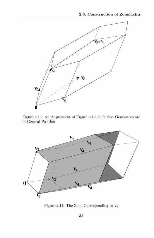
2.6. Construction of Zonohedra
v3
v1
v2
0
v4
v3 v4+
Figure 2.13: An Adjustment of Figure 2.12, such that Generators arein General Position
v1
v2
v3
0
v4
v4v4
v4
v4 v4v4
Figure 2.14: The Zone Corresponding to v4
35
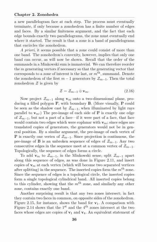
Chapter 2. Zonohedra
a new parallelogram face at each step. The process must eventuallyterminate, if only because a zonohedron has a finite number of edgesand faces. By a similar finiteness argument, and the fact that eachedge bounds exactly two parallelograms, the zone must eventually endwhere it started. The result is that a zone is a band of parallelogramsthat encircles the zonohedron.
A priori, it seems possible that a zone could consist of more thanone band. The zonohedron’s convexity, however, implies that only oneband can occur, as will now be shown. Recall that the order of thesummands in a Minkowski sum is immaterial. We can therefore reorderthe m generating vectors if necessary so that the generating vector thatcorresponds to a zone of interest is the last, or m
th, summand. Denotethe zonohedron of the first m ≠ 1 generators by Zm≠1. Then the totalzonohedron Z is given by
Z = Zm≠1 ü vm. (2.16)
Now project Zm≠1 along vm onto a two-dimensional plane, pro-ducing a filled polygon P, with boundary B. (More visually, P couldbe seen as the shadow cast by Zm≠1, when illuminated by light raysparallel to vm.) The pre-image of each side of P is exactly one edgeof Zm≠1, but not a part of a face—if it were part of a face, that facewould contain two edges which were coplanar with vm; since edges aretranslated copies of generators, the generators would not be in gen-eral position. By a similar argument, the pre-image of each vertex ofP is exactly one vertex of Zm≠1. Since projection is continuous, thepre-image of B is an unbroken sequence of edges of Zm≠1. Any twoconsecutive edges in the sequence meet at a common vertex of Zm≠1.Topologically, the sequence of edges forms a circle.
To add vm to Zm≠1, in the Minkowski sense, split Zm≠1 apartalong this sequence of edges, as was done in Figure 2.11, and insertcopies of vm at each vertex (which will become two separated verticesafter splitting) in the sequence. The inserted copies form the m
th zone.Since the sequence of edges is a topological circle, the inserted copiesform a single topological cylindrical band. All inserted copies belongto this cylinder, showing that the m
th zone, and similarly any otherzone, contains exactly one band.
Another surprising result is that any two zones intersect; in factthey contain two faces in common, on opposite sides of the zonohedron.Figure 2.15, for instance, shows the band for v1. A comparison withFigure 2.14 shows that the 1st and the 4th zones intersect at the twofaces whose edges are copies of v1 and v4. An equivalent statement of
36

2.7. Zonohedra as Convex Polytopes
v1
v2
v3
0
v4v1
v1
v1
v1
v1v1
Figure 2.15: The Zone Corresponding to v1
this result is that, for any pair of generators vi and vj , a zonohedroncontains two parallelogram faces whose edges are translations of vi
and vj . Again, an argument from construction makes this result clear.Begin the construction of the zonohedron with vi and vj , so the firststage will be a parallelogram with edges vi and vj . The Minkowski sumwith the third generator will be a parallelepiped, two opposite faces ofwhich are ij-parallelograms. Further Minkowski sums will add morezones to the zonohedron, and will maintain those two faces, thoughmoving them steadily farther apart. The faces will remain after thezonohedron is complete, and the ith and jth zones will each containboth of them.
2.7 Zonohedra as Convex PolytopesBoth geometric and algebraic arguments show that a zonohedron isa convex polytope. Geometrically, the method of construction showsthat a zonohedron’s boundary consists of a finite number of line seg-ments and parallelogram faces, both of which consist of convex combi-nations of their vertices. Since there are finitely many edges and faces,there are also finitely many vertices, which generate all the edges andfaces, not to mention the solid zonohedron itself.
Algebraically, Equation (2.11) can be rewritten in terms of the set
37
Chapter 2. Zonohedra
of nodes:
Z(G) = hull(N (Z)). (2.17)
To see this result, express the zonotope in the form given in Equation(2.11). Any point p in the zonotope can be then be expressed by asequence –1, –2, ..., –m of coe�cients in that equation, where each –i
is between 0 and 1. Formally,
p =mÿ
i=1–ivi (2.18)
= –1v1 + –2v2 + ... + –mvm. (2.19)
Note that this expression might not be unique—often many such se-quences define the same point.
Without loss of generality, the vectors v1, v2, ..., vm can be re-ordered if necessary so that
–1 Æ –2 Æ –3 Æ ... Æ –m. (2.20)
To show that Z is the convex hull of the nodes of Z, it is su�cient toexpress p as a convex combination of a set of nodes. In other words,write p as a linear combination of nodes, whose coe�cients are allbetween 0 and 1, and all sum to 1. To write p in this form, rearrangeEquation (2.19):
p = –1
mÿ
i=1vi + (–2 ≠ –1)
mÿ
i=2vi + ...
... + (–3 ≠ –2)mÿ
i=3vi + ... + (–m ≠ –m≠1)
mÿ
i=m
vi (2.21)
=mÿ
j=1
Q
a(–j ≠ –j≠1)mÿ
i=j
vi
R
b , (2.22)
where –0 is set to 0. Each summation inside the parentheses in Equa-tion (2.22) is a sum of generating vectors, so, by Equation (2.15), theyare all nodes. Furthermore, the inequalities in Equation (2.20) insurethat each coe�cient inside the parentheses is between 0 and 1. Thesum of all the coe�cients inside the parentheses is a telescoping series
–1 + –2 ≠ –1 + –3 ≠ –2 + ... + –m≠1 ≠ –m≠2 + –m ≠ –m≠1, (2.23)
38
2.8. Coe�cient Sequences for Zonohedra
which sums to –m.Equation (2.22) nearly achieves our goal of writing p as a sum of
nodes, with coe�cients between 0 and 1, that sum to 1. To take thefinal step, use the fact that the zero vector 0 is always in the set ofnodes, and add a multiple of 0 to Equation (2.22):
p =mÿ
j=1
Q
a(–j ≠ –j≠1)mÿ
i=j
vi
R
b + (1 ≠ –m)0. (2.24)
This addition does not change the vector produced by the linear com-bination of nodes, but does guarantee that its coe�cients sum to 1, asneeded. We have therefore succeeded in writing a point p as a convexcombination of nodes.
The nodes in Equation (2.22) are all sums of sequences of vectorsin G, where the sequences have di�erent lengths. What constitutes a“sequence,” however, depends on how the vectors in G are ordered,and the ordering used for Equation (2.22) was chosen to insure thatEquation (2.20) held. The –i’s in Equation (2.18) could be chosen toinduce any desired ordering, so the entire set of orderings, and thusthe entire set of nodes, is needed.
The constructions show that every vertex of a zonohedron is thesum of a set of generating vectors, so every vertex is a node. Evensimple examples, however, like the zonogon in Figure 2.6 show thatnot every node is a vertex—in fact, many nodes occur in the interior.
The fact that a zonohedron, or in fact a general zonotope, is theconvex hull of its finite set of nodes establishes that a zonotope is aconvex polytope. This result will allow us to reach conclusions aboutpossible coordinate representations of points in zonotopes, and, in laterchapters, those representations will imply that some colours can onlybe produced in certain ways.
2.8 Coe�cient Sequences for ZonohedraEquation (2.11) expresses a point p in a zonotope by a sequence
(–1, –2, ..., –m), (2.25)
where the –’s are the coe�cients in a linear combination of generatingvectors that produces p. As simple examples like Figure 2.6 show, thatsequence might not be unique. In fact, when there are more generators
39
Chapter 2. Zonohedra
than dimensions, there is often a multitude of such sequences. A se-quence could be used as a set of coordinates for a point in a zonotope.This section shows that, under the assumption of general position, apoint on the boundary of a zonohedron has a unique coordinate se-quence. The result is first shown for the zonohedron’s vertices, each ofwhich can be written, in just one way, as the sum of all the generatingvectors which lie on one side of a hyperplane through the origin. Thatresult is then used to derive similar uniqueness results for points onedges or faces.
2.8.1 Vertices
Section 2.7 showed that a zonotope is a convex polytope and Section1.3.4 explained that the vertices of a convex polytope are exposedpoints: for each vertex v there exists a supporting hyperplane Hv suchthat Hv intersects the polytope only at v; apart from that intersection,the polytope lies completely on one side of Hv. This section will provefrom that description that each vertex of a zonotope is representedby a unique coordinate sequence. The coordinate sequence containsonly 0s and 1s, so each vertex is the sum of a unique subset of thegenerating vectors, consisting of those that are on one side of Hv,after translating Hv to the origin.
The proof interprets a vertex as the solution to an optimizationproblem that is studied in linear programming: find a point pmax ona convex polytope at which a given linear functional takes on a maxi-mum value. Section 1.2 characterized a linear functional as a stack ofparallel hyperplanes, each of which is the pre-image under that func-tional of a certain real number. The functional values correspondingto a hyperplane increase as the hyperplanes get further from the ori-gin. Geometrically, then, pmax must lie on a supporting hyperplane;all the hyperplanes on one side are of smaller value, and none of thehyperplanes on the other side intersect the polytope.
In the case at hand, the polytope is a zonotope Z. Let us specify avertex v, and find its coordinate sequence. First, choose a supportinghyperplane Hv. The hyperplane defines, up to a scalar factor, a func-tional Fv; choose the scalar factor so that Fv(Hv) is positive. By theargument in the previous paragraph, v is the unique solution to theproblem of maximizing Fv over Z.
Every point in Z has the form given by Equation (2.11), so we can
40
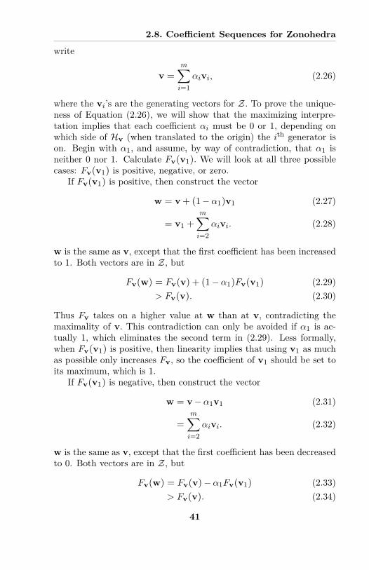
2.8. Coe�cient Sequences for Zonohedra
write
v =mÿ
i=1–ivi, (2.26)
where the vi’s are the generating vectors for Z. To prove the unique-ness of Equation (2.26), we will show that the maximizing interpre-tation implies that each coe�cient –i must be 0 or 1, depending onwhich side of Hv (when translated to the origin) the i
th generator ison. Begin with –1, and assume, by way of contradiction, that –1 isneither 0 nor 1. Calculate Fv(v1). We will look at all three possiblecases: Fv(v1) is positive, negative, or zero.
If Fv(v1) is positive, then construct the vector
w = v + (1 ≠ –1)v1 (2.27)
= v1 +mÿ
i=2–ivi. (2.28)
w is the same as v, except that the first coe�cient has been increasedto 1. Both vectors are in Z, but
Fv(w) = Fv(v) + (1 ≠ –1)Fv(v1) (2.29)> Fv(v). (2.30)
Thus Fv takes on a higher value at w than at v, contradicting themaximality of v. This contradiction can only be avoided if –1 is ac-tually 1, which eliminates the second term in (2.29). Less formally,when Fv(v1) is positive, then linearity implies that using v1 as muchas possible only increases Fv, so the coe�cient of v1 should be set toits maximum, which is 1.
If Fv(v1) is negative, then construct the vector
w = v ≠ –1v1 (2.31)
=mÿ
i=2–ivi. (2.32)
w is the same as v, except that the first coe�cient has been decreasedto 0. Both vectors are in Z, but
Fv(w) = Fv(v) ≠ –1Fv(v1) (2.33)> Fv(v). (2.34)
41
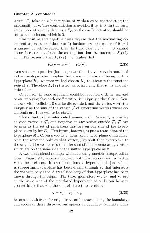
Chapter 2. Zonohedra
Again, Fv takes on a higher value at w than at v, contradicting themaximality of v. The contradiction is avoided if –1 is 0. In this case,using more of v1 only decreases Fv, so the coe�cient of v1 should beset to its minimum, which is 0.
The positive and negative cases require that the maximizing co-e�cient –1 must be either 0 or 1; furthermore, the choice of 0 or 1is unique. It will be shown that the third case, Fv(v1) = 0, cannotoccur, because it violates the assumption that Hv intersects Z onlyat v. The reason is that Fv(v1) = 0 implies that
Fv(v + –1v1) = Fv(v), (2.35)
even when –1 is positive (but no greater than 1). v+–1v1 is containedin the zonotope, which implies that v+–1v1 is also on the supportinghyperplane Hv, whereas we had chosen Hv to intersect the zonotopeonly at v. Therefore Fv(v1) is not zero, implying that –1 is uniquelyeither 0 or 1.
Of course, the same argument could be repeated with –2, –3, andso on, implying that each coe�cient –1 is uniquely either 0 or 1. Gen-erators with coe�cient 0 can be disregarded, and the vertex v writtenuniquely as the sum of the subset GÕ of generating vectors whose co-e�cients are 1, as was to be shown.
This subset can be interpreted geometrically. Since Fv is positiveon each vector in GÕ, and negative on any vector outside GÕ, GÕ canbe seen as the set of generators that are on one side of the hyper-plane given by ker Fv. This kernel, however, is just a translation of thehyperplane Hv. Given a vertex v, then, and a hyperplane which inter-sects the zonotope only at that vertex, just shift that hyperplane tothe origin. The vertex v is then the sum of all the generating vectorswhich are on the same side of the shifted hyperplane as v.
A two-dimensional example will make the geometric interpretationclear. Figure 2.16 shows a zonogon with five generators. A vertexv has been chosen. In two dimensions, a hyperplane is just a line.A supporting hyperplane has been drawn through v, that intersectsthe zonogon only at v. A translated copy of that hyperplane has beendrawn through the origin. The three generators v1, v3, and v4 areon the same side of the translated hyperplane as v. It can be seengeometrically that v is the sum of these three vectors:
v = v1 + v3 + v4, (2.36)
because a path from the origin to v can be traced along the boundary,and copies of those three vectors appear as boundary segments along
42
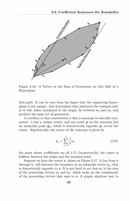
2.8. Coe�cient Sequences for Zonohedra
v1
v2
v3
v1
v2
v3
v3
v5
v4
v4
v4
v5
v5 Supp
ortin
g Hyp
erpl
ane
Tran
slated
Hyp
erpl
ane
v
Figure 2.16: A Vertex as the Sum of Generators on One Side of aHyperplane
that path. It can be seen from the figure that the supporting hyper-plane is not unique. Any hyperplane that intersects the zonogon onlyat v will, when translated to the origin, lie between v4 and v5, andproduce the same set of generators.
A corollary to this construction is that a zonotope is centrally sym-metric: it has a unique center, and any point p on the zonotope hasan antipodal point pa, which is diametrically opposite p, across thecenter. Algebraically, the center of the zonotope is given by
vc =mÿ
1=1
12vi, (2.37)
the point whose coe�cients are all 1/2. Geometrically, the center ishalfway between the origin and the terminal point.
Suppose we have the vertex v, shown in Figure 2.17. A line from vthrough vc will intersect the boundary at an antipodal vertex va, thatis diametrically opposite to v. It is not hard to see that va is the sumof the generating vectors v2 and v5, which make up the complementof the generating vectors that sum to v. A simple algebraic way to
43
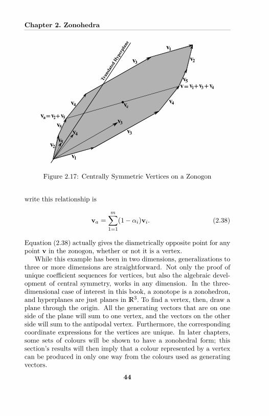
Chapter 2. Zonohedra
v1
v2v3
v1
v2
v3
v3
v5
v4
v4
v4
v5
v5
v1+ +v3 v4
Tran
slated
Hyp
erpl
ane
v2+ v5
v
vc
= va
=
Figure 2.17: Centrally Symmetric Vertices on a Zonogon
write this relationship is
va =mÿ
1=1(1 ≠ –i)vi. (2.38)
Equation (2.38) actually gives the diametrically opposite point for anypoint v in the zonogon, whether or not it is a vertex.
While this example has been in two dimensions, generalizations tothree or more dimensions are straightforward. Not only the proof ofunique coe�cient sequences for vertices, but also the algebraic devel-opment of central symmetry, works in any dimension. In the three-dimensional case of interest in this book, a zonotope is a zonohedron,and hyperplanes are just planes in R3. To find a vertex, then, draw aplane through the origin. All the generating vectors that are on oneside of the plane will sum to one vertex, and the vectors on the otherside will sum to the antipodal vertex. Furthermore, the correspondingcoordinate expressions for the vertices are unique. In later chapters,some sets of colours will be shown to have a zonohedral form; thissection’s results will then imply that a colour represented by a vertexcan be produced in only one way from the colours used as generatingvectors.
44
2.8. Coe�cient Sequences for Zonohedra
2.8.2 Edges and FacesThe previous section showed that each vertex of a zonotope has aunique expression as a linear combination of the generating vectors.This section proves similar results for edges and faces, except thatuniqueness is no longer automatic; rather, it now requires the gener-ating vectors to satisfy some linear independence relationships. For-tunately, the requirements are mild: as long as no two generators arescalar multiples of each other, each point on an edge has a unique coef-ficient sequence, and as long as no three generating vectors are linearlydependent, each point on a face has a unique coe�cient sequence. Forzonohedra, both these conditions are satisfied when the generators arein general position, which is the generic case. Geometrically, generalposition implies that all a zonohedron’s faces are parallelograms, andthat each edge is a translated copy of a single generator (rather thanmultiple generators laid end to end).
The result about edges will be proven first. Assume, for a givenzonohedron Z(G), that no two vectors in G are linearly dependent,i.e. that no two vectors are scalar multiples of each other.. Let E bean edge of Z, and let vE be the generator of which E is a copy. Theassumption that no two generators are linearly dependent implies thatvE is a unique, single vector. (The only other option is that E consistsof multiple generators laid end to end, but that configuration requirestwo or more generators to be linearly dependent.)
As an edge, E is bounded by two vertices, w1 and w2. Reorder thevertices if necessary so that
w1 + vE = w2. (2.39)
To show that any point wE on E has a unique coordinate sequence,begin by choosing a supporting hyperplane HE that contains the edgeE , but that does not otherwise intersect Z; in particular, HE containsno face of Z. The existence of such an HE follows from the fact thatZ is a convex polytope.
Translate HE to the origin, and consider its relationship to thegenerating vectors. First, since E is a translated copy of vE , it followsthat vE is contained in the translated HE . Second, since w1 and w2are bounding vertices, it follows from previous discussions that HEcorresponds to a linear functional fE that is maximized by w1 and w2.The translated HE divides G into three subsets: G+ (the generatorson which FE is positive), G≠ (the generators on which FE is negative),and vE (the single generator on which FE is zero).
45
Chapter 2. Zonohedra
We can write w1 and w2 in terms of these subsets:
w1 =ÿ
viœG+
vi, (2.40)
w2 =ÿ
viœG+fivE
vi. (2.41)
Since w1 and w2 are vertices, these expressions are unique. Everypoint wE on E can be written as
wE = –w1 + (1 ≠ –)w2, (2.42)
for some unique – between 0 and 1. Then, since w1 + vE = w2, wecan write
wE = w1 + –vE (2.43)
=ÿ
viœG+
vi + –vE . (2.44)
Equation (2.44) provides one coe�cient sequence for wE ; unique-ness follows from the maximizing behavior of FE . Since w1 and w2both maximize the linear functional FE , therefore wE , which is a con-vex combination of w1 and w2, also maximizes FE . From Equation(2.44) we can write
FE (wE ) = FE
Q
aÿ
viœG+
vi
R
b + FE (–vE ). (2.45)
Eliminating any vector in G+, or reducing its coe�cient to less than1, in the first argument on the right of Equation (2.45), would onlydecrease the value of FE . Similarly, introducing any vector in G≠, orincreasing its coe�cient beyond 0, would only cause a decrease. There-fore, all coe�cients for G+ must remain at 1, and all coe�cients forG≠ must remain at 0. Increasing or decreasing – would not changethe value of FE , but would invalidate Equation (2.43), so – must alsostay the same. The expression in Equation (2.44) is therefore the onlyone possible, so every point on the edge of a zonotope, under the as-sumption that no two generators are linearly dependent, must have aunique coe�cient sequence, as was to be shown.
Uniqueness will now be proven similarly for points on a zonotope’sface, under the assumption that no three generating vectors are lin-early dependent. The edge E is replaced with a face F , and the hy-perplane HF makes full contact with that face, but with no other
46
2.8. Coe�cient Sequences for Zonohedra
part of the zonotope. Again, translate HF to the origin. Define FF ,G+, and G≠ similarly to the edge case. Instead of just containing onegenerator vE , the translated hyperplane now contains two generators,vF1 and vF2. Any other generator that might be contained in thetranslated hyperplane would be a linear combination of vF1 and vF2,which would violate the assumption; therefore vF1 and vF2 are theonly generators in the translated hyperplane.
Since the face F consists, after translation, of zonal combinationsof two vectors, it is a parallelogram with four vertices. One of thevertices, which we’ll call w1, is an “initial” vertex, and the oppositevertex, which we’ll call w2, is a “terminal” vertex. These two verticessatisfy the relationship
w2 = w1 + vF1 + vF2. (2.46)
The remaining two vertices of the parallelogram are w1 + vF1 andw1 + vF2. The linear independence of vF1 and vF2 imply that, forany point wF on the face, there exist two unique constants, –1 and–2, both between 0 and 1, such that
wF = w1 + –1vF1 + –2vF2. (2.47)
As before, the vertex w1 is a unique linear combination of generators,whose indices are taken from some subset G+, so we have
wF =ÿ
viœG+
vi + –1vF1 + –2vF2. (2.48)
Again, apply FF to both sides of Equation (2.48). Argue as beforethat the coe�cients for generators in G+ and G≠ cannot be changed.The two remaining coe�cients, –1 and –2, are unique because vF1and vF2 are linearly independent; this reasoning is a two-dimensionalversion of the reasoning after Equation (2.45), where there was onlycoe�cient –, instead of two. Since all the coe�cients in Equation(2.48) are unique, any point on the face of a zonotope, or in particular azonohedron, provided that no three generators are linearly dependent,has a unique coe�cient sequence, as was to be shown.
A simple corollary of these two proofs can also be seen. The uniquecoe�cient sequence for a point on the edge of a zonotope consistsentirely of zeros and ones, except for at most one generator. Similarly,the unique coe�cient sequence for a point on the face of a zonotopeconsists entirely of zeros and ones, except for at most two generators.Both these corollaries, of course, make an appropriate general positionassumption.
47
Chapter 2. Zonohedra
2.9 Cyclic Zonohedra
Cyclic zonohedra are non-negative zonohedra whose generators forma minimal set for their convex cone. They occur several times incolour science, and the cyclic property is vital to some results. Thissection describes cyclic zonohedra, presents a convenient constructionfor them, and shows that they possess some regularities that makethem easy to work with.
Formally, suppose we have a set G of m non-negative generatingvectors. They can be pictured as line segments emerging from theorigin, in the non-negative octant of R3. Each generating vector canbe extended to a semi-infinite ray, and the convex hull of those raysis the convex cone, cone(G), of the generating set. Although the term“cone” suggests a regular, usually circular, profile, a cone in this con-text could have a very irregular profile; since there are only finitelymany generating rays, the profile must be polygonal.
Regardless of its profile, any finitely-generated convex cone stillhas an inside, a surface, and an outside. Typically, one pictures acone’s generating rays as lying on its surface. Possibly, however, oneor more of the rays is inside the cone. In that case, any rays that areinside are not needed to generate the cone. Geometrically, the insiderays are convex combinations of the rays on the surface and so areunnecessary; the generators as a whole, then, do not form a minimalset for the cone.
While this discussion has been in three dimensions, Figure 2.18shows that the issues can be expressed more clearly in two dimensions.The left side of the figure shows five non-negative generators, theirextension to rays, and the convex cone that results. A simple way toview the profile of the cone, and to determine whether any rays areinside, is to slice it with the plane H given by x + y + z = 1. Theresult appears on the right of the figure. Each generator produces onepoint pi on the plane x+ y + z = 1. Denote the set of points pi by P.
In that plane, the convex hull, hull(P), of the pi’s is a polygon. Itis easy to see that a ray created from a generating vector is inside theconvex cone if and only the corresponding point is inside the polygon;in the figure, for instance, the ray through v3 can be written as a con-vex combination of the rays through the other four generators, and p3can be written as a convex combination of the other four points. (An-other interpretation is that a ray is inside the convex cone if and onlyif the corresponding generator is a non-negative linear combination ofthe other generators.) It is also easy to see that the choice of sec-
48
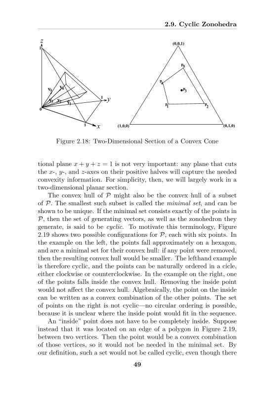
2.9. Cyclic Zonohedra
v1v2v3
v4v5
1
1
1 x
y
z
01 2
p3
4
5
p
p
pp
(1,0,0) (0,1,0)
(0,0,1)
Figure 2.18: Two-Dimensional Section of a Convex Cone
tional plane x + y + z = 1 is not very important: any plane that cutsthe x-, y-, and z-axes on their positive halves will capture the neededconvexity information. For simplicity, then, we will largely work in atwo-dimensional planar section.
The convex hull of P might also be the convex hull of a subsetof P. The smallest such subset is called the minimal set, and can beshown to be unique. If the minimal set consists exactly of the points inP, then the set of generating vectors, as well as the zonohedron theygenerate, is said to be cyclic. To motivate this terminology, Figure2.19 shows two possible configurations for P, each with six points. Inthe example on the left, the points fall approximately on a hexagon,and are a minimal set for their convex hull: if any point were removed,then the resulting convex hull would be smaller. The lefthand exampleis therefore cyclic, and the points can be naturally ordered in a cicle,either clockwise or counterclockwise. In the example on the right, oneof the points falls inside the convex hull. Removing the inside pointwould not a�ect the convex hull. Algebraically, the point on the insidecan be written as a convex combination of the other points. The setof points on the right is not cyclic—no circular ordering is possible,because it is unclear where the inside point would fit in the sequence.
An “inside” point does not have to be completely inside. Supposeinstead that it was located on an edge of a polygon in Figure 2.19,between two vertices. Then the point would be a convex combinationof those vertices, so it would not be needed in the minimal set. Byour definition, such a set would not be called cyclic, even though there
49
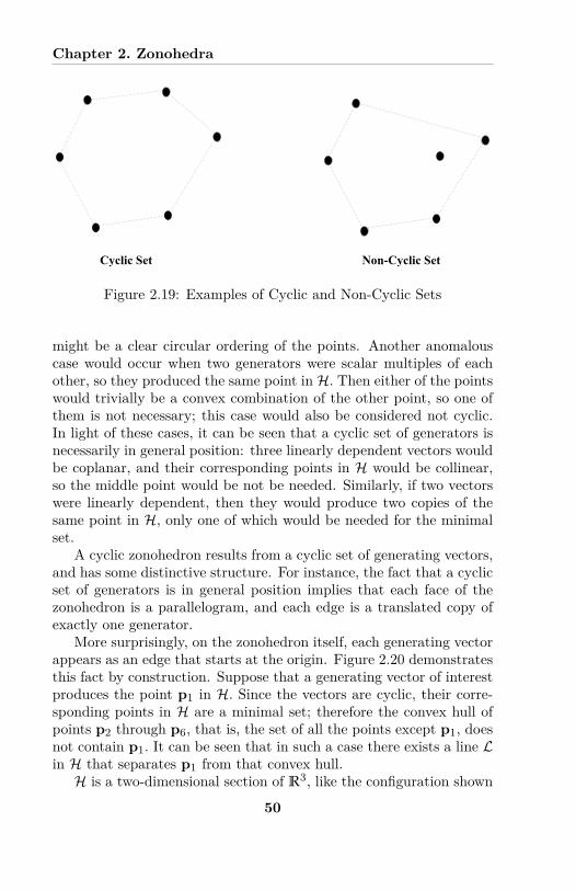
Chapter 2. Zonohedra
Cyclic Set Non-Cyclic Set
Figure 2.19: Examples of Cyclic and Non-Cyclic Sets
might be a clear circular ordering of the points. Another anomalouscase would occur when two generators were scalar multiples of eachother, so they produced the same point in H. Then either of the pointswould trivially be a convex combination of the other point, so one ofthem is not necessary; this case would also be considered not cyclic.In light of these cases, it can be seen that a cyclic set of generators isnecessarily in general position: three linearly dependent vectors wouldbe coplanar, and their corresponding points in H would be collinear,so the middle point would be not be needed. Similarly, if two vectorswere linearly dependent, then they would produce two copies of thesame point in H, only one of which would be needed for the minimalset.
A cyclic zonohedron results from a cyclic set of generating vectors,and has some distinctive structure. For instance, the fact that a cyclicset of generators is in general position implies that each face of thezonohedron is a parallelogram, and each edge is a translated copy ofexactly one generator.
More surprisingly, on the zonohedron itself, each generating vectorappears as an edge that starts at the origin. Figure 2.20 demonstratesthis fact by construction. Suppose that a generating vector of interestproduces the point p1 in H. Since the vectors are cyclic, their corre-sponding points in H are a minimal set; therefore the convex hull ofpoints p2 through p6, that is, the set of all the points except p1, doesnot contain p1. It can be seen that in such a case there exists a line Lin H that separates p1 from that convex hull.
H is a two-dimensional section of R3, like the configuration shown
50
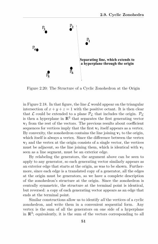
2.9. Cyclic Zonohedra
1
Separating line, which extends to a hyperplane through the origin
p
2p3p
4p
5p6p
Figure 2.20: The Structure of a Cyclic Zonohedron at the Origin
in Figure 2.18. In that figure, the line L would appear on the triangularintersection of x + y + z = 1 with the positive octant. It is then clearthat L could be extended to a plane PL that includes the origin. PLis then a hyperplane in R3 that separates the first generating vectorv1 from the rest of the vectors. The previous results about coe�cientsequences for vertices imply that the first v1 itself appears as a vertex.By convexity, the zonohedron contains the line joining v1 to the origin,which itself is always a vertex. Since the di�erence between the vertexv1 and the vertex at the origin consists of a single vector, the verticesmust be adjacent, so the line joining them, which is identical with v1seen as a line segment, must be an exterior edge.
By relabeling the generators, the argument above can be seen toapply to any generator, so each generating vector similarly appears asan exterior edge that starts at the origin, as was to be shown. Further-more, since each edge is a translated copy of a generator, all the edgesat the origin must be generators, so we have a complete descriptionof the zonohedron’s structure at the origin. Since the zonohedron iscentrally symmetric, the structure at the terminal point is identical,but reversed: a copy of each generating vector appears as an edge thatends at the terminal point.
Similar constructions allow us to identify all the vertices of a cycliczonohedron, and write them in a convenient sequential form. Anyvertex is the sum of all the generators on one side of a hyperplanein R3; equivalently, it is the sum of the vectors corresponding to all
51
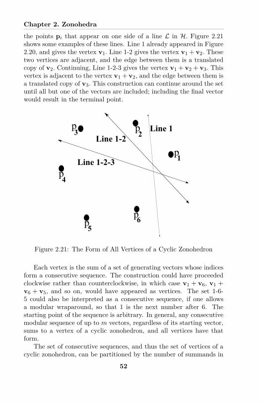
Chapter 2. Zonohedra
the points pi that appear on one side of a line L in H. Figure 2.21shows some examples of these lines. Line 1 already appeared in Figure2.20, and gives the vertex v1. Line 1-2 gives the vertex v1 + v2. Thesetwo vertices are adjacent, and the edge between them is a translatedcopy of v2. Continuing, Line 1-2-3 gives the vertex v1 + v2 + v3. Thisvertex is adjacent to the vertex v1 + v2, and the edge between them isa translated copy of v3. This construction can continue around the setuntil all but one of the vectors are included; including the final vectorwould result in the terminal point.
6
Line 1Line 1-2
Line 1-2-3 1p
2p3
p
4p
5p
p
Figure 2.21: The Form of All Vertices of a Cyclic Zonohedron
Each vertex is the sum of a set of generating vectors whose indicesform a consecutive sequence. The construction could have proceededclockwise rather than counterclockwise, in which case v1 + v6, v1 +v6 + v5, and so on, would have appeared as vertices. The set 1-6-5 could also be interpreted as a consecutive sequence, if one allowsa modular wraparound, so that 1 is the next number after 6. Thestarting point of the sequence is arbitrary. In general, any consecutivemodular sequence of up to m vectors, regardless of its starting vector,sums to a vertex of a cyclic zonohedron, and all vertices have thatform.
The set of consecutive sequences, and thus the set of vertices of acyclic zonohedron, can be partitioned by the number of summands in
52
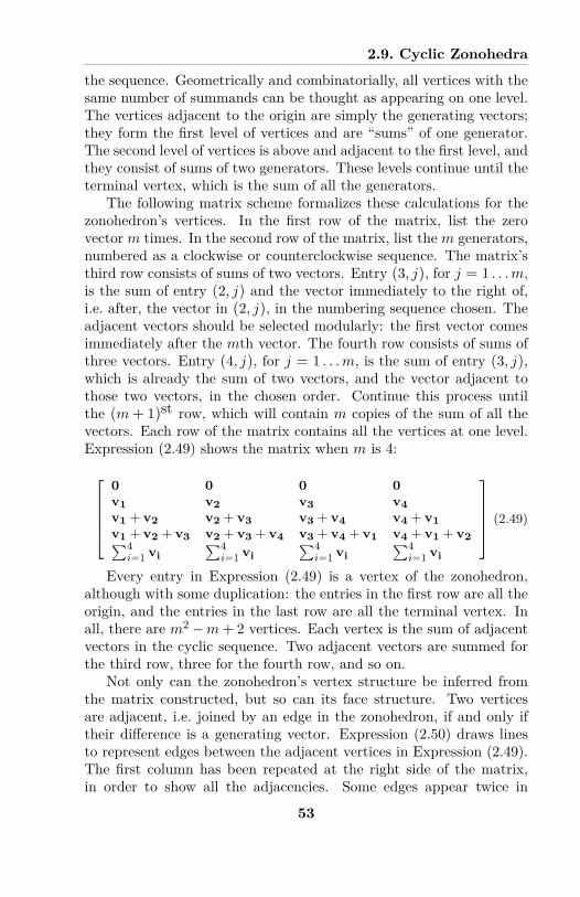
2.9. Cyclic Zonohedra
the sequence. Geometrically and combinatorially, all vertices with thesame number of summands can be thought as appearing on one level.The vertices adjacent to the origin are simply the generating vectors;they form the first level of vertices and are “sums” of one generator.The second level of vertices is above and adjacent to the first level, andthey consist of sums of two generators. These levels continue until theterminal vertex, which is the sum of all the generators.
The following matrix scheme formalizes these calculations for thezonohedron’s vertices. In the first row of the matrix, list the zerovector m times. In the second row of the matrix, list the m generators,numbered as a clockwise or counterclockwise sequence. The matrix’sthird row consists of sums of two vectors. Entry (3, j), for j = 1 . . . m,is the sum of entry (2, j) and the vector immediately to the right of,i.e. after, the vector in (2, j), in the numbering sequence chosen. Theadjacent vectors should be selected modularly: the first vector comesimmediately after the mth vector. The fourth row consists of sums ofthree vectors. Entry (4, j), for j = 1 . . . m, is the sum of entry (3, j),which is already the sum of two vectors, and the vector adjacent tothose two vectors, in the chosen order. Continue this process untilthe (m + 1)st row, which will contain m copies of the sum of all thevectors. Each row of the matrix contains all the vertices at one level.Expression (2.49) shows the matrix when m is 4:
S
WWWU
0 0 0 0
v1 v2 v3 v4v1 + v2 v2 + v3 v3 + v4 v4 + v1v1 + v2 + v3 v2 + v3 + v4 v3 + v4 + v1 v4 + v1 + v2q4
i=1 viq4
i=1 viq4
i=1 viq4
i=1 vi
T
XXXV(2.49)
Every entry in Expression (2.49) is a vertex of the zonohedron,although with some duplication: the entries in the first row are all theorigin, and the entries in the last row are all the terminal vertex. Inall, there are m
2 ≠ m + 2 vertices. Each vertex is the sum of adjacentvectors in the cyclic sequence. Two adjacent vectors are summed forthe third row, three for the fourth row, and so on.
Not only can the zonohedron’s vertex structure be inferred fromthe matrix constructed, but so can its face structure. Two verticesare adjacent, i.e. joined by an edge in the zonohedron, if and only iftheir di�erence is a generating vector. Expression (2.50) draws linesto represent edges between the adjacent vertices in Expression (2.49).The first column has been repeated at the right side of the matrix,in order to show all the adjacencies. Some edges appear twice in
53
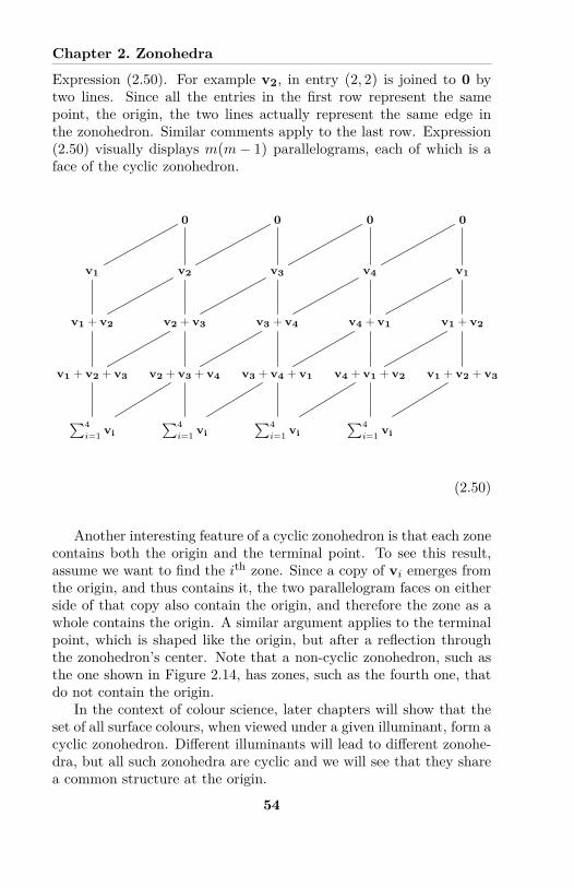
Chapter 2. Zonohedra
Expression (2.50). For example v2, in entry (2, 2) is joined to 0 bytwo lines. Since all the entries in the first row represent the samepoint, the origin, the two lines actually represent the same edge inthe zonohedron. Similar comments apply to the last row. Expression(2.50) visually displays m(m ≠ 1) parallelograms, each of which is aface of the cyclic zonohedron.
0 0 0 0
v1 v2 v3 v4 v1
v1 + v2 v2 + v3 v3 + v4 v4 + v1 v1 + v2
v1 + v2 + v3 v2 + v3 + v4 v3 + v4 + v1 v4 + v1 + v2 v1 + v2 + v3
q4i=1 vi
q4i=1 vi
q4i=1 vi
q4i=1 vi
(2.50)
Another interesting feature of a cyclic zonohedron is that each zonecontains both the origin and the terminal point. To see this result,assume we want to find the i
th zone. Since a copy of vi emerges fromthe origin, and thus contains it, the two parallelogram faces on eitherside of that copy also contain the origin, and therefore the zone as awhole contains the origin. A similar argument applies to the terminalpoint, which is shaped like the origin, but after a reflection throughthe zonohedron’s center. Note that a non-cyclic zonohedron, such asthe one shown in Figure 2.14, has zones, such as the fourth one, thatdo not contain the origin.
In the context of colour science, later chapters will show that theset of all surface colours, when viewed under a given illuminant, form acyclic zonohedron. Di�erent illuminants will lead to di�erent zonohe-dra, but all such zonohedra are cyclic and we will see that they sharea common structure at the origin.
54
2.10. Chapter Summary
2.10 Chapter SummaryThis chapter has presented two important constructions, Minkowskisums and zonohedra (more generally, zonotopes), and derived someuseful properties about them. This summary lists the definitions andresults.
Definition of the Minkowski Sum. The Minkowski sum, denotedü, of two non-empty subsets, A and B, of a vector space Rn, is definedas
A ü B =)
vA + vB--vA œ A and vB œ B
*. (2.51)
Properties of the Minkowski Sum:
1. The Minkowski sum of an arbitrary number of summands is well-defined, and is independent of the order of those summands.
2. The Minkowski sum of an arbitrary number of convex sets isagain a convex set.
Definitions for Zonotopes and Zonohedra:
1. Suppose that we have a set of vectors G = {v1, v2, ..., vm}, inRn. The zonotope Z generated by G is the Minkowski sum of theline segments corresponding to those vectors:
Z(G) = v1 ü v2 ü ... ü vm. (2.52)
Equivalently, Z(G) can be written as
Z(G) =I
mÿ
i=1–ivi
-----0 Æ –i Æ 1 ’i
J. (2.53)
If n = 2, then Z is a zonogon. If n = 3, then Z is a zonohedron.2. A zonotope is non-negative if there exists a basis of Rn in which
all the co-ordinates, of every vector in G, are non-negative. Anon-negative zonotope has a terminal point, given by
v1 + v2 + ... + vm, (2.54)
and a center, given bymÿ
1=1
12vi. (2.55)
55
Chapter 2. Zonohedra
3. Suppose that v is one of the generators for a zonohedron Z.Then the zone of Z corresponding to v consists of all the facesof Z for which one edge is a translated copy of v.
4. A set of vectors G in Rn is in general position if every subset ofn vectors in G is linearly independent.
5. A set of non-negative vectors G in R3 is cyclic if no vector inG is contained within the convex cone of the other vectors. Azonohedron Z(G) that results from a cyclic generating set is alsocalled cyclic.
Properties of Zonotopes and Zonohedra:
1. A zonotope is a convex polytope, with a polytope’s usual struc-ture of vertices, edges, k-dimensional faces, and so on.
2. If a zonohedron’s generators are in general position, then(a) Each edge of the zonohedron is a translated copy of one and
only one of the generators, and(b) Each face of the zonohedron is a parallelogram; further-
more, each edge of any such parallelogram is a translatedcopy of one of the generators.
3. The converse to Result 2 holds: if each edge of a zonohedron is atranslated copy of a generator, and each face of the zonohedron isa parallelogram, then the zonohedron’s generators are in generalposition.
4. A zonotope is centrally symmetric: the pointsmÿ
1=1–ivi and
mÿ
1=1(1 ≠ –i)vi (2.56)
on the zonotope are the endpoints of a line segment whosehalfway mark is the zonotope’s center.
5. If v is a vertex of a zonotope, then there is a unique sequenceof –i’s in Equation (2.53), which produce v. Each –i in that se-quence is either a 0 or a 1. Furthermore, a hyperplane H throughthe origin can be found, such that any generator with coe�cient1 is on one side of H, and any generator with coe�cient 0 is onthe other side.
6. The converse to Result 5 holds. Suppose the hyperplane Hthrough the origin contains no vector in the generating set G.Then the sum of all the generators on either side of H is a ver-tex of Z(G).
56
2.10. Chapter Summary
7. Suppose no two generating vectors are linearly dependent, andthat v is on an edge of the zonotope produced by the generatingvectors. Then there is a unique sequence of –i’s in Equation(2.53), which produce v. At most one –i is strictly between 0and 1; every other coe�cient is either 0 or 1.
8. Suppose the generating vectors for a zonohedron in R3 are ingeneral position (i.e no subset of three is linearly dependent),and that v is on the boundary of the zonohedron produced bythe generating vectors. Then there is a unique sequence of –i’s inEquation (2.53), which produce v. At most two –i’s are strictlybetween 0 and 1; every other coe�cient is either 0 or 1.
9. Suppose a zonohedron is cyclic. Then each generating vectoroccurs as an edge that starts at the origin, and these are theonly edges that emerge from the origin.
10. Similarly, each generating vector occurs as an edge that ends atthe terminal point, and these are the only edges that end at theterminal point.
11. Each zone of a cyclic zonohedron contains both the origin andthe terminal point.
12. The vertices of a cyclic zonohedron have a special form. Let thegenerating vectors be numbered cyclically (either clockwise orcounterclockwise) from 1 to m. Then a sum of generating vectorsis a vertex if and only if the indices of those generating vectorsform a consecutive sequence. This sequence can be modular;for instance, {m ≠ 1, m, 1, 2} would be considered a consecutivesequence.
13. The matrix pattern in Expression (2.50), when generalized tom entries rather than just four, gives the complete structure ofvertices, edges, and faces for a cyclic zonohedron.
57

Chapter 2. Zonohedra
58
Chapter 3
Physical Factors inColour Matching
3.1 Introduction
Both physical and perceptual factors contribute to human colour sen-sations. The perceptual factors result from the human visual system(HVS), including the eyes, the brain, and the optic nerve, and possi-bly involve psychological properties too. The physical factors behindcolour, on the other hand, are independent of a human subject. Theyinclude the light sources which make vision possible, and the opticalproperties of perceived objects. In both theory and practice, these twofactors are distinct. This chapter deals with physical factors; the nextchapter deals with perceptual factors.
In an everyday viewing situation, a human’s field of view consistsof a scene with many objects, at various di�erent locations. Some dis-tribution of light enters the eyes from each direction. The distributionof light from a particular direction will be referred to as a colour stim-ulus or visual stimulus. A visual scene contains a multitude of colourstimuli, each of which, when interpreted by the human visual system,produces a colour sensation. Equivalently, a scene is a set of coloursensations, where each direction provides one stimulus.
A basic question is how these stimuli relate to the colours theyproduce. Colour science approaches this question by starting withsimple cases, and moving to progressively more complicated cases—we will see, however, that even uncomplicated cases require elaborate
59
Chapter 3. Physical Factors in Colour Matching
analysis. In the simplest case, a viewer sees only a single stimulus,from a uniform patch of colour, against a “‘black” background, wherethere is no light at all. In such experiments, observers can assigna hue (red, yellow, green, etc.) and a saturation (dull, vivid, etc.)to a stimulus. Even the hues, though, are limited: for example, nobrowns or greys can be produced. Furthermore, since the eye adaptsto the ambient illumination level, one cannot usually say whether thestimulus is bright or dim.
The simplest case after an isolated stimulus—and the case of in-terest for this book—consists of two uniform patches of colour, viewedagainst a black background. The patches appear side by side. Typ-ically they are both semicircles that together form a complete circle,subtending about 2¶ of the field of view, about the same angle sub-tended by a thumb held out at arm’s length. The two colour patchescan now be compared visually. In some cases, the colours look iden-tical, or match, even though the two stimuli are physically di�erent.Viewers in these colour-matching experiment adjust one of the stimuliuntil the two colours agree. By systematically varying the stimuli, andtesting many human subjects, a substantial body of colour-matchingdata has been accumulated, which was codified in the 1931 StandardObserver, by the Commission Internationale de l’Éclairage (CIE). De-spite their simplicity, colour-matching experiments lead to a rich veinof perceptual and geometric analysis, which this book works out in de-tail. Colour matching is basic to many important, and more advanced,topics in colour science, which this book will not treat, but for whichit will lay a solid foundation.
This chapter begins the analysis of colour matching by examiningcolour stimuli: the physical light that enters the eye and produces acolour perception. While some colour stimuli travel directly from aphysical light source to a perceiving eye, a more important case oc-curs when a stimulus results from light that leaves a source, and thenreflects o� an intermediate object, before finally reaching a humanperceiver. The elements of this case are handled separately. First,light is considered solely as a radiometric power density over the vis-ible spectrum. The shape of a density, independent of its magnitude,is described by an illuminant. An object’s reflectance properties aregiven by its reflectance spectrum, which is a function that takes onvalues between 0 and 100% over the visible spectrum, and describeshow much light of each wavelength is reflected. Radiometric densi-ties, illuminants, and reflectance spectra all have natural vector spacestructures, which this chapter formalizes. Later chapters will find
60
3.2. Colour Stimuli
transformations from these physical vector spaces to perceptual andsensor vector spaces. The images of the transformations will lead to ge-ometric constructions, including zonohedra, in the destination spaces.
3.2 Colour Stimuli3.2.1 Radiometric FunctionsThe human visual system responds to light, which is electromag-netic radiation in the visible spectrum, where wavelengths are betweenabout 400 and 700 nm; a visual or colour stimulus consists of light (pro-vided its composition is constant for some reasonable time period) thatreaches a human eye. A colour stimulus can be adequately describedfor colour science by the amount of power it contains at a limited setof wavelengths ⁄, or in a set of narrow wavelength bands. The unitof power is the Watt (W), so a colour stimulus will be modeled as afunction that assigns a certain number of Watts to each wavelength,or wavelength band, in the visible spectrum. Such a function is calleda spectral power density (SPD). (Technically, the power of a stimulusin a certain wavelength band is given by integrating the SPD overthat band, and a stimulus is a measure, in the mathematical sense ofmeasure theory. For our purposes, however, the common conceptionof an SPD as a function will su�ce.) Figure 3.1 graphs an exam-ple of a colour stimulus given by an SPD. The horizontal axis is thewavelength, and the vertical axis is power.
In practical situations, the power or intensity of a stimulus is con-sidered not just on its own, but in context, and the units of the verticalaxis in Figure 3.1 change accordingly, although the change is typicallyunstated. An SPD, for instance, might be impinging on a piece ofpaper. Since the SPD delivers some amount of power to each area ofthe paper, natural units are Watts per square meter (W/m2). On theother hand, an SPD might occur as the output of a light bulb, whichis modeled as a point source. Then a solid angle centered at the bulbcontains a certain amount of light, so natural units are Watts per stera-dian (W/sr). In many contexts, a stimulus has multiple simultaneousinterpretations. For instance, a light bulb emits an SPD, which thenilluminates a piece of paper. Even though they have di�erent units,the emitted and the illuminating SPD have the same shape. Ratherthan make multiple SPD graphs with di�erent units, only one graph ismade, with no units given. Radiometry deals with the interaction ofSPDs and objects, and the appropriate units, so the terms radiometric
61
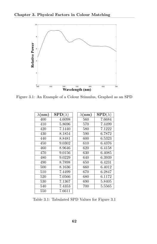
Chapter 3. Physical Factors in Colour Matching
Wavelength (nm)
Rel
ativ
e Po
wer
0
2
4
6
8
10
400 450 500 550 600 650 700
Figure 3.1: An Example of a Colour Stimulus, Graphed as an SPD
⁄(nm) SPD(⁄) ⁄(nm) SPD(⁄)400 4.6098 560 7.6684410 5.8696 570 7.4499420 7.1440 580 7.1222430 8.1854 590 6.7872440 8.8481 600 6.5323450 9.0302 610 6.4376460 8.9646 620 6.4158470 9.0156 630 6.4085480 9.0229 640 6.3939490 8.7898 650 6.4231500 8.1636 660 6.4012510 7.4499 670 6.2847520 7.0566 680 6.1172530 7.1367 690 5.8405540 7.4353 700 5.5565550 7.6611
Table 3.1: Tabulated SPD Values for Figure 3.1
62
3.2. Colour Stimuli
function, SPD, colour stimulus, and visual stimulus (or just stimulus)will be used as synonyms.
Though they are often drawn as continuous functions, colour stim-uli are typically given as discrete tabulations. Table 3.1, for examplecontains the same data as Figure 3.1, but listed at 31 wavelengths,running from 400 to 700 nm in intervals of 10 nm. A 10 nm resolutionis fine enough to account for most colour phenomena, so this book willtreat colour stimuli as discrete functions over those 31 wavelengths.Adjustments can easily be made for finer or coarser resolutions.
3.2.2 Colour Stimuli as a Subset of a Vector SpaceBecause of the relatively low wavelength resolution needed, a vectorspace formulation of colour stimuli is both su�cient for colour scienceand computationally convenient. Throughout this book, therefore, the31 power levels for a colour stimulus will be interpreted as the entries ofa 31-dimensional vector. Each colour stimulus can equivalently be seenas a non-negative discrete function of the visible spectrum, over thewavelengths 400 nm, 410 nm, ..., 700 nm. The set S of colour stimulican be viewed as a subset of the 31-dimensional real vector space S ofdiscrete functions which take on arbitrary values at those wavelengths.This underlying vector space structure will be used extensively later,for further definitions and for geometric constructions.
Addition and scalar multiplication of the radiometric functions in Sare consistent with the vector space operations in S, and have naturalphysical interpretations. Addition corresponds to superposition. Sup-pose for instance that a piece of paper is illuminated simultaneouslyby two SPDs. Then the total illumination is a third SPD, which is themathematical sum of the first two; physically, two stimuli have beensuperposed to produce a new stimulus. Scalar multiplying an SPDby a constant k corresponds to changing the SPD’s absolute powerlevels while retaining its relative power levels; the graph will changeits size, but not its shape. An obvious example is a dimmer switch fora light bulb, which increases or decreases brightness without changingthe relative power outputs at di�erent wavelengths.
The set S of SPDs is only a subset, and not a subspace, of the vectorspace S, because functions in S can take on negative values. A vector inS is a physically possible SPD if and only if all its coordinates—whichrepresent physical power levels—are non-negative. While a vector withsome negative coordinates has no physical meaning, it is still usefulmathematically, and we will later define some linear transformations
63
Chapter 3. Physical Factors in Colour Matching
on S, with the understanding that they are physically meaningful onlywhen restricted to S. Working with the larger space S allows us toapply the machinery of linear algebra, which will later prove essentialfor derivations.
While the coordinates for a vector space are arbitrary, an obviouschoice of coordinates for S is the power levels at the 31 wavelengths400 nm, 410 nm, ..., 700 nm. The corresponding basis vector for eachcoordinate is an indicator function, which take on the value 1 at thatwavelength, and the value 0 everywhere else. Formally, define
‡400(⁄) =
I1, if ⁄ = 400,0, otherwise, (3.1)
to be the indicator function for 400 nm, and define other basis vectorssimilarly. The units of ‡400 are chosen appropriately for the context.Such indicator functions are called monochromatic. As a whole, theset of indicator functions serve as a basis for S.
The total power of a radiometric function is an important physicalconcept, with a natural interpretation as a linear functional P on thevector space S. Define P first on basis vectors and then extend it toall vectors by linearity:
P (‡⁄) = 1, (3.2)
where ⁄ is any of the 31 basis wavelengths. The linearity of P isactually a physical statement, rather than a mathematical statement,relying on the fact that SPDs can be superposed without interacting.Later, another important functional on S, the luminance functionalY , will be seen to be perceptual rather than physical.
3.3 Illuminants and Light SourcesSome kind of light source or illumination is needed to produce a colourstimulus. A light source can produce a stimulus either directly, forexample when a viewer looks right at a lit light bulb, or indirectly, forexample after the light from a source reflects o� some physical object.In either case, the SPD of the illuminating light a�ects the SPD ofthe stimulus reaching a human observer, and thus a�ects the resultingcolour perception. This section discusses illuminants and light sources,two colour science terms that are relevant to illumination.
In typical everyday viewing, a light source or sources illuminate ascene containing multiple objects. Suppose for simplicity that there is
64
3.3. Illuminants and Light Sources
a single light source, or, if there are multiple light sources, then theyall have SPDs of the same shape. Obvious examples are an outdoorscene which is illuminated solely by the sun, or an indoors room thatis lit by a multitude of identical fluorescent tubes. In either of thesearrangements, the intensity of the lighting will vary greatly at di�erentpoints and in di�erent directions, due to the spreading of the light asit leaves the source, superposition of light from multiple sources, andshadows cast by some objects on other objects. In addition, a stronglydirectional source, such as the sun on a clear day, sheds much morelight on the parts of objects that are facing the sun, and much less onthe parts that are turned away from the sun.
In this example, the SPDs of the sunlight that reaches di�erentparts of the scene vary greatly in intensity, but their shapes, that is,the relative power at various wavelengths, would not vary much. In adistinction that is not always observed, colour science applies the termilluminant to the relative SPD of illuminating light and the term lightsource to a physical object or phenomenon that produces that light.Any source, regardless of its intensity, whose SPD has the shape of agiven illuminant, is said to be consistent with that illuminant. Twosources, such as a 100 W and a 200 W incandescent bulb, can thus havedi�erent magnitudes, yet, since their SPDs have the same shape, beconsistent with the same illuminant. Another common example occursas emitted light gets progressively farther from a point source such asa candle flame: the light’s power decreases as the inverse square of thedistance from the flame, but its SPD keeps the same shape.
Over the years, a series of standard illuminants has been defined.Illuminant A, shown in Figure 3.2 with two other illuminants, modelslight from incandescent sources. Illuminant C is an average of indi-rect daylight. Illuminant E has equal power at every wavelength. Thevertical units in Figure 3.2 are arbitrary: they could be multiplied byany scalar constant without changing the illuminant. As with SPDsthemselves, practical experience has shown that a 10 nm resolutionis adequate to model illuminants for colour science. Thus an illumi-nant I will be treated as a 31-dimensional vector, over the same 31wavelengths used previously. More precisely, an illuminant is an equiv-alence class of 31-dimensional vectors that are scalar multiples of oneanother, and which thus produce the same shape when graphed; thislevel of precision, however, is usually not needed. As 31-dimensionalvectors, illuminants can be seen as elements of S. Since an illuminant’spower is non-negative at any wavelength, illuminants can also be writ-ten as elements of the set S of physically possible SPDs, and inherit
65

Chapter 3. Physical Factors in Colour Matching
400 450 500 550 600 650 7000
1
2
3
4
5
6
7
Wavelength (nm)
Rel
ativ
e Po
wer
A
C
E
Figure 3.2: Some Standard Illuminants
the same natural vector space operations.At various points in this book, an illuminant will be required to be
positive, meaning that it has positive power at every wavelength; itsgraph over the visible spectrum never takes on the value 0. This mainlytechnical condition avoids degenerate cases. In practice, positivenessis the norm, because most light sources, especially natural ones, dohave some power at every wavelength. Exceptions occur of course inartificial situations, such as a monochromator that outputs light ofa very narrow bandwidth. Geometric constructions might also usetheoretical illuminants given by monochromatic SPDs.
3.4 Reflectance SpectraWhile some colour stimuli reach the eye when humans view a lightsource directly, for example by looking at the sun or a burning lightbulb, stimuli more commonly result when lighting interacts with theobjects in a scene before arriving at a human eye. Often, in fact, thelight source is not even within the field of view. The most frequentform of interaction is Lambertian reflection, also called matte or di�usereflection, which works on the various wavelengths independently. ALambertian object absorbs a certain percentage of the incoming light
66
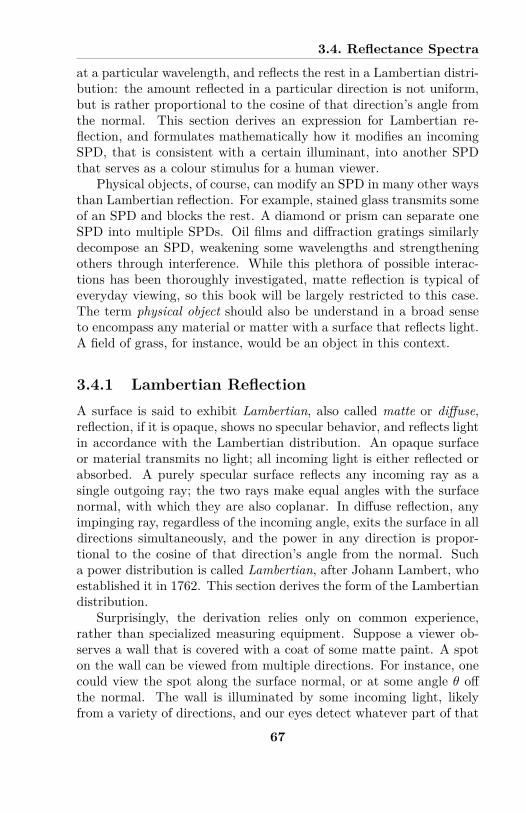
3.4. Reflectance Spectra
at a particular wavelength, and reflects the rest in a Lambertian distri-bution: the amount reflected in a particular direction is not uniform,but is rather proportional to the cosine of that direction’s angle fromthe normal. This section derives an expression for Lambertian re-flection, and formulates mathematically how it modifies an incomingSPD, that is consistent with a certain illuminant, into another SPDthat serves as a colour stimulus for a human viewer.
Physical objects, of course, can modify an SPD in many other waysthan Lambertian reflection. For example, stained glass transmits someof an SPD and blocks the rest. A diamond or prism can separate oneSPD into multiple SPDs. Oil films and di�raction gratings similarlydecompose an SPD, weakening some wavelengths and strengtheningothers through interference. While this plethora of possible interac-tions has been thoroughly investigated, matte reflection is typical ofeveryday viewing, so this book will be largely restricted to this case.The term physical object should also be understand in a broad senseto encompass any material or matter with a surface that reflects light.A field of grass, for instance, would be an object in this context.
3.4.1 Lambertian ReflectionA surface is said to exhibit Lambertian, also called matte or di�use,reflection, if it is opaque, shows no specular behavior, and reflects lightin accordance with the Lambertian distribution. An opaque surfaceor material transmits no light; all incoming light is either reflected orabsorbed. A purely specular surface reflects any incoming ray as asingle outgoing ray; the two rays make equal angles with the surfacenormal, with which they are also coplanar. In di�use reflection, anyimpinging ray, regardless of the incoming angle, exits the surface in alldirections simultaneously, and the power in any direction is propor-tional to the cosine of that direction’s angle from the normal. Sucha power distribution is called Lambertian, after Johann Lambert, whoestablished it in 1762. This section derives the form of the Lambertiandistribution.
Surprisingly, the derivation relies only on common experience,rather than specialized measuring equipment. Suppose a viewer ob-serves a wall that is covered with a coat of some matte paint. A spoton the wall can be viewed from multiple directions. For instance, onecould view the spot along the surface normal, or at some angle ◊ o�the normal. The wall is illuminated by some incoming light, likelyfrom a variety of directions, and our eyes detect whatever part of that
67
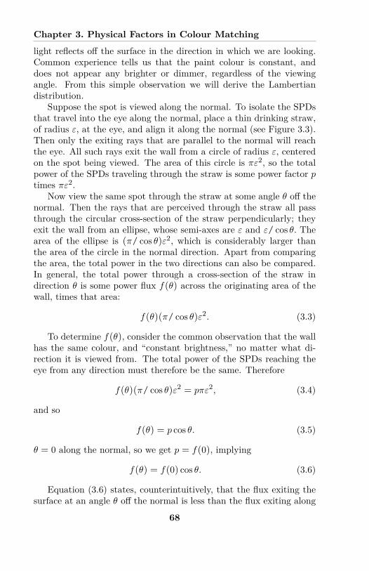
Chapter 3. Physical Factors in Colour Matching
light reflects o� the surface in the direction in which we are looking.Common experience tells us that the paint colour is constant, anddoes not appear any brighter or dimmer, regardless of the viewingangle. From this simple observation we will derive the Lambertiandistribution.
Suppose the spot is viewed along the normal. To isolate the SPDsthat travel into the eye along the normal, place a thin drinking straw,of radius Á, at the eye, and align it along the normal (see Figure 3.3).Then only the exiting rays that are parallel to the normal will reachthe eye. All such rays exit the wall from a circle of radius Á, centeredon the spot being viewed. The area of this circle is fiÁ
2, so the totalpower of the SPDs traveling through the straw is some power factor p
times fiÁ
2.Now view the same spot through the straw at some angle ◊ o� the
normal. Then the rays that are perceived through the straw all passthrough the circular cross-section of the straw perpendicularly; theyexit the wall from an ellipse, whose semi-axes are Á and Á/ cos ◊. Thearea of the ellipse is (fi/ cos ◊)Á2, which is considerably larger thanthe area of the circle in the normal direction. Apart from comparingthe area, the total power in the two directions can also be compared.In general, the total power through a cross-section of the straw indirection ◊ is some power flux f(◊) across the originating area of thewall, times that area:
f(◊)(fi/ cos ◊)Á2. (3.3)
To determine f(◊), consider the common observation that the wallhas the same colour, and “constant brightness,” no matter what di-rection it is viewed from. The total power of the SPDs reaching theeye from any direction must therefore be the same. Therefore
f(◊)(fi/ cos ◊)Á2 = pfiÁ
2, (3.4)
and so
f(◊) = p cos ◊. (3.5)
◊ = 0 along the normal, so we get p = f(0), implying
f(◊) = f(0) cos ◊. (3.6)
Equation (3.6) states, counterintuitively, that the flux exiting thesurface at an angle ◊ o� the normal is less than the flux exiting along
68
3.4. Reflectance Spectra
Surface
Reflected
Rays
Straw Along Non-Normal
/cos
Stra
w A
long
Nor
mal
Reflected Rays
Surface
Figure 3.3: Reflected Rays in Di�erent Directions
the normal, by a factor of cos ◊. The di�erence can be significant:almost no power exits in directions that are nearly parallel to the sur-face. Figure 3.4 shows the relative amount of power flux in one planethrough the normal. The length of the arrow in the direction given bythe angle ◊ from the normal is proportional to the flux that exits inthat direction. From Equation (3.6), it can be calculated that the tipsof the arrows lie on a circle that is tangent to the surface. This circlejust gives the results for one plane; to be extended to three-dimensionalspace, rotate the circle around the normal to make a sphere. In ra-diometry, the definition of radiance, referring to the light emitted bya surface such as a computer monitor, includes the factor cos ◊; ourderivations motivate this often unexplained factor.
The physical mechanism behind the Lambertian distribution re-quires another distinction, between first-surface reflectance and bulkreflectance. In first-surface reflectance, a ray reflects o� the surface ofan object without entering the object. In bulk reflectance, a ray entersthe object before it is reflected. Once inside the object, it interactswith a variety of atoms or molecules, and can be scattered in manydirections. The various photons of the ray take randomly determinedpaths, that can be wildly di�erent. Some paths will cause photons toexit the object through the surface. The exiting photons can be trav-eling in many di�erent directions, with no relation to their incoming
69
Chapter 3. Physical Factors in Colour Matching
Surface
Reflected Rays
Figure 3.4: Lambertian Reflectance Distribution in a Plane Containingthe Normal
direction. The observed Lambertian exiting distribution likely has astatistical explanation, but the details seem not to be well understood.
In practice, many surfaces that are mostly matte exhibit a slightgloss component, in which light that arrives at a certain angle to thenormal, such as 30¶, is reflected specularly, but light at any other angleis reflected di�usely. Gloss causes a highlight, sometimes sharp andsometimes blurry, that reflects the light source and moves on the sur-face as the viewer changes position. Both matte and gloss componentscan be encompassed in a bi-directional reflectance distribution function(BRDF). Suppose we fix an incoming direction and an outgoing direc-tion, and shine an SPD towards the surface along the incoming direc-tion. Then some percentage (perhaps 0) of the incoming power will bereflected in the outgoing direction. The BRDF gives that percentage,for every pair of incoming and outgoing directions. While they arethe most comprehensive description of surface reflections, BRDFs aredi�cult to measure and cumbersome to calculate with. Though com-prehensive, they are rarely necessary, because the gloss component ofmost surfaces is often small enough to be neglected.
This book restricts itself to opaque objects whose reflectance issolely di�use. Gloss, transparency, iridescence, fluorescence, and soon, will not be treated. Though some interesting phenomena are elim-inated, the case that is treated is in some sense the norm. A proto-typical example of di�use reflectance is acrylic paint, for either artistsor housepainters, with a matte finish; these paints alone fill out theuniverse of object colours fairly well.
70
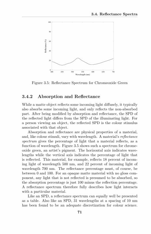
3.4. Reflectance Spectra
0
20
40
60
80
100
400 450 500 550 600 650 700
Ref
lect
ance
(%)
Wavelength (nm)
Figure 3.5: Reflectance Spectrum for Chromeoxide Green
3.4.2 Absorption and ReflectanceWhile a matte object reflects some incoming light di�usely, it typicallyalso absorbs some incoming light, and only reflects the non-absorbedpart. After being modified by absorption and reflectance, the SPD ofthe reflected light di�ers from the SPD of the illuminating light. Fora person viewing an object, the reflected SPD is the colour stimulusassociated with that object.
Absorption and reflectance are physical properties of a material,and, like colour stimuli, vary with wavelength. A material’s reflectancespectrum gives the percentage of light that a material reflects, as afunction of wavelength. Figure 3.5 shows such a spectrum for chrome-oxide green, an artist’s pigment. The horizontal axis indicates wave-lengths while the vertical axis indicates the percentage of light thatis reflected. This material, for example, reflects 18 percent of incom-ing light of wavelength 500 nm, and 22 percent of incoming light ofwavelength 700 nm. The reflectance percentage must, of course, bebetween 0 and 100. For an opaque matte material with no gloss com-ponent, any light that is not reflected is presumed to be absorbed, sothe absorption percentage is just 100 minus the reflection percentage.A reflectance spectrum therefore fully describes how light interactswith a particular material.
Like an SPD, a reflectance spectrum can equally well be presentedas a table. Also like an SPD, 31 wavelengths at a spacing of 10 nmhas been found to be an adequate discretization for colour science.
71
Chapter 3. Physical Factors in Colour Matching
As before, we can construct a vector space, which we will call R, ofall the functions at the 31 wavelengths, with no restrictions on thosefunctions’ values. The reflectance spectra make up a subset R of R,where R consists of all functions with values between 0 and 100%.Equivalently, R consists of all functions with values between 0 and1. A material’s reflectance spectrum will be typically denoted as afunction fl(⁄), where ⁄ represents wavelength.
The set of reflectance functions has two natural limits, describedas ideal black and ideal white. An ideal black reflectance functionreflects 0% of the incoming light at every wavelength, while ideal whitereflects 100%. Ideal black would be the darkest surface that couldpossibly exist, while an ideal white surface, also called an ideal di�usereflector would be the brightest. These two extremes have been closelyapproximated in practice, but not quite attained. Nevertheless, theyare useful for theoretical and mathematical analysis.
The vector space R has a natural basis, analogous to the monochro-matic basis for S. The maximal monochromatic reflectance (MMR)spectrum at wavelength ⁄, denoted fl⁄, is defined to take on the value100% at ⁄, and the value 0 elsewhere. For example, the maximalmonochromatic spectrum at 600 nm is given by
fl600(⁄) =
I1, if ⁄ = 600,0, otherwise. (3.7)
Physically, such a material would reflect light only at the wavelength600 nm (or at the wavelength band containing 600 nm), and absorblight of any other wavelength. We will use M to denote the set ofthe 31 MMR spectra, which form a vector space basis for R. Unlikemonochromatic SPDs, which are easily produced by a monochromatoror lasers, no materials with MMR spectra are currently known to exist.Any one that did exist would be very dark, because it would only reflecta small portion (1/31st) of the incoming light.
Since reflectance produces a modified SPD from an incoming SPD,a spectrum fl can also be seen as a transformation from the vector spaceS to itself. No confusion will result if fl denotes both the spectrum andthe transformation. Of course, this transformation is physically mean-ingful only when restricted to the set S of SPDs, which fl preserves.It is easy to see that fl is a diagonal linear operator. The applicationof fl to an incoming SPD ‡ can be written in matrix form:
72
3.5. Chapter Summary
fl(‡) =
S
WWU
fl(400) 0 . . . 0 00 fl(410) . . . 0 0
. . . . . . . . . . . . . . .0 0 . . . fl(690) 00 0 . . . 0 fl(700)
T
XXV
S
WWU
‡(400)‡(410)
. . .‡(690)‡(700)
T
XXV (3.8)
=
S
WWU
fl(400)‡(400)fl(410)‡(410)
. . .fl(690)‡(690)fl(700)‡(700)
T
XXV . (3.9)
The last line gives the power levels, at each wavelength, of the colourstimulus resulting from an object of reflectance spectrum fl, when il-luminated by an SPD ‡. The expression shows that it is produced byelement-wise multiplication of fl and ‡’s vector representations in Rand S.
3.5 Chapter SummaryThis chapter has formalized mathematically the physical aspects ofcolour that are needed for analyzing colour matches. The main objectsintroduced were colour stimuli (or equivalently, radiometric functions,or SPDs), illuminants, and reflectance spectra. All these objects werecast as elements of appropriate vector spaces. To define any of theseobjects with enough accuracy for colour science, it is su�cient to writethem as discrete functions over the set of 31 wavelengths, obtained bygoing from 400 nm to 700 nm (the boundaries of the visible spectrum)in steps of 10 nm.
More formally, the following terms were defined:
1. The 31-dimensional real vector space S of power level functionson the 31 wavelengths,
2. The monochromatic SPDs ‡⁄, which take on the value 1 at wave-length ⁄ and the value 0 elsewhere, form a basis for S,
3. The set S of colour stimuli. S is the subset, though not the sub-space, of S that consists of all non-negative functions on the 31wavelengths. Physically, the non-negative functions correspondto SPDs, which are emitted by light sources and modified by ma-terial objects. An SPD that enters an observer’s eye is thought ofas a colour stimulus, because it can produce a colour sensation,
4. An SPD is said to be positive if it takes on only positive values,and no negative or zero values, over the entire visible spectrum,
73
Chapter 3. Physical Factors in Colour Matching
5. An illuminant I is a relative SPD; it defines the shape of an SPD,but not its magnitude. Any SPD sharing that shape is said tobe consistent with the illuminant. An illuminant could also bethought of as an equivalence class of SPDs, where two SPDs areequivalent if they are multiples of each other,
6. The 31-dimensional real vector space R of reflectance functionson the 31 wavelengths,
7. The set M of 31 maximal monochromatic reflectance (MMR)spectra fl⁄, which take on the value 100% at wavelength ⁄ andthe value 0 elsewhere; they form a basis for R,
8. The set R of reflectance spectra. R is the subset, though notthe subspace, of R that consists of all functions on the 31 wave-lengths that take on values between 0 and 100%. Each element fl
of R can also be seen as a diagonal linear operator on S. Mathe-matically, a material with reflectance spectrum fl will modify anSPD that strikes it, in accordance with this operator. Physically,the material absorbs some percentage of each wavelength of theincoming SPD and di�usely reflects the remaining percentage.The materials of interest for this book are assumed to be opaqueand to interact with light only through absorption and di�usereflectance.
74
Index
10¶ Standard Observer, 792¶ Standard Observer, 790-1 function, 145, 1491931 CIE Standard Observer,
see StandardObserver
Abney’s Laws, 75, 86–88, 116absorption, 67, 71–74additivity, 80, 87, 115, 116a�ne subspace, 101, 188annulus, 145antipodal point, 43aperture viewing, 77, 78, 115,
132, 157associativity, 19
basic solution, 191basis ray, 10, 101, 103, 105,
107Bezold-Brücke e�ect, 134bi-directional reflectance
distribution function(BRDF), 70
black-and-white movie, 83,163
boundary colours (of display),209–211
boundary point, ii, 120, 144,147, 149, 153, 155,
173, 190, 195,210–212
brightness, 75, 88, 106, 115Brill, Michael H., 123Broadbent, A. D., 92, 93brown, 77
camera, see sensorcenter, see zonotope, centerchevron, 6chroma, Munsell, 81, 134chromaticity, 120, 128–134,
144, 149, 153, 155,169, 174, 182, 198,205
coordinate, 130, 168diagram, ii, 120, 128,
131–134, 144, 147,149, 154, 160, 168,169, 176, 195, 200,211
gamut, 198–203, 211interpretation, 133–134ray, 128, 144, 149, 155,
201chromeoxide green, 71CIE, see Commission
Internationale del’Éclairage
213
INDEX
CIE coordinates, seetristimuluscoordinates
closed set, 6colour
appearance, i, 76, 88constancy, 77, 121,
157–159, 173conversion, 184–187, 194correction, 159, 160,
177–178, 180matching, i, ii, 1, 18, 60,
75–117, 124, 138neutral, 133optimal, ii, iii, 120, 123,
144–155, 211perception, 1, 59, 73,
75–117, 125, 203related, 77science, i, 17, 60, 75, 119signal map, 164, 183, 192space, ii, 17, 75, 115, 120,
123, 125, 128, 160,164, 172, 183, 192,198, 211
stimulus, ii, 1, 59, 61–64,66, 73, 75, 77, 86,115, 119–121, 125,128, 129, 135, 152,159, 161, 167, 169,173, 176, 180, 204
surface or object, 23, 119,121–122, 129, 137,147, 157, 160, 164,178, 193
colour-matching algebra,79–88
colour-matching experiment,77–79, 89, 97, 115,161, 163
colour-matching functions, 76,
88–98, 101, 105–113,117, 124, 126, 137,154, 160, 163, 164,172, 176, 187
combinationconvex, 5, 7, 15, 37, 38,
120, 132, 179linear, 7, 17, 25, 48, 138,
154, 167, 172, 210non-negative, 9zonal, 24, 47, 119, 152,
153, 172, 203, 207,209, 210, 212
combinatorics, 14, 16, 31, 53,139, 149, 150
Commission Internationale del’Éclairage, ii, 60, 76,78, 89, 105
commutativity, 19computational colour
constancy, ii,157–194
cone, 181convex, see convex,coneimproper, 10, 104inside, surface, outside, 48long-wave, mid-wave,
short-wave, 81profile, 48proper, 10, 101, 102, 104,
105red, green, blue, 81, 159spectrum, see spectrum
conevisual, 81, 124, 159, 183
constancy, see colourconstancy orcomputational colourconstancy
constant brightness, 68constraint, 189–191
214
INDEX
continuity, 205, 209control sequence, 197, 203–211convex
combination, seecombination, convex
cone, ii, 2, 8–11, 13, 15,23, 48, 56, 76, 101,103, 104, 107, 108,116, 120, 125–127,139, 142, 154, 155,165, 166, 193, 210
hull, 6–8, 11, 13, 15, 48,127, 132, 179, 188
polytope, 2, 11–12, 15,17, 37–39, 45, 56,188, 190, 194
set, 5–12, 15, 17, 19, 55convexity, ii, 1–16, 36, 119,
144, 175, 201and colour matching,
101–105coordinates for zonotope, see
zonotope orzonohedron,coe�cient sequences
Coxeter, H. S. M., iiicube, 10, 13, 101, 103, 125,
188cyclic set of vectors, 49, 120,
123, 127, 139, 145,147, 149, 154, 155,160, 165, 167, 172,210
cyclic zonohedron, seezonohedron, cyclic
daytime vision, 81decomposition, 26density, 60diamond, 6di�use reflection, see
reflection,Lambertian
dilation, 181direction, 165, 168, 174discrete, 211display gamut, ii, iii, 23, 134,
157–195, 198, 201,204, 211
display spectrum cone, 202dissection, iii, 195, 203–205,
207, 209, 212dot product, 14
electromagnetic spectrum, seespectrum,electromagnetic
electronic display, 195–212electronic display gamut, see
display gamutenergy e�ciency, 203, 209, 212equal-energy stimulus, 76, 77,
105, 110, 117equality, 189equivalence, 80, 86, 115, 116
class, 65relationship, 80
Euclidean space, 5, 14, 16, 179exposed point, 12, 16exposure time, 173
field of view, 59, 77, 159filter, 177flicker photometry, 83fluorescence, 70foliation, 4, 15Forsyth, David, 177, 179functional, linear, see linear
functional
gain, 173gamma correction, 197gamut, see display gamut
215
INDEX
gamut-based illuminantestimation (GBIE),160, 177–183, 193
GBIE, see gamut-basedilluminant estimation(GBIE)
general position, 28–29, 32–34,40, 45, 50, 56, 144,172
generating vectors, seegenerators
generators, 40, 48, 55direction, 31, 123, 127,
139, 142for convex cone, 8for convex hull, 7for polytope, 12for zonohedron, see
zonohedron,generators
for zonotope, seezonotope, generators
magnitude, 31, 127, 139,142
geometric construction, 63,119–155, 192, 204
gloss, 70, 178Grassmann’s Laws, 75, 79–82,
88, 90, 92, 115Grassmann, Hermann, 79grey, 77, 191grey world assumption, 182
half-space, 3, 4, 10, 11heterochromatic, 83highlight, 70, 178hue, 60, 79, 81, 82, 113, 133human visual system, 59, 61,
78, 83, 160, 163, 169hyperplane, 2–5, 14, 27, 40, 56
a�ne, 3, 14, 102, 107
luminance, 106–108supporting, 9, 12, 40, 45,
102, 104, 188
ideal black, 72, 100, 137, 145,151, 155, 179, 197,200
ideal di�use reflector, 72ideal white, 72, 135, 137, 142,
145, 150, 182illuminant, 54, 60, 64–67, 73,
119, 122, 125, 126,129, 135, 144,147–149, 152, 154,155, 160, 164–166,168, 171, 192
A, 65, 174, 191C, 65D65, 157, 180, 191, 199,
205D75, 178E, 65, 84, 163, 174estimation, 177–178F1, 157metameric, 143positive, 66, 125, 126,
134, 139, 140, 144,154, 155, 166, 171,175, 193
standard, 65illuminant gamut, ii, iii, 160,
161, 171–177, 179,180, 193
power level scaling,173–174
power scaling, 181shape at origin, 174–176,
181, 193illumination, 60, 64, 66, 84,
129, 134, 135, 157,164
216
INDEX
image gamut, 177–179, 193imaginary primaries, 89, 113,
132, 169improper cone, see cone,
improperindependence, linear, see
linear independenceindicator function, 64inequality, 189ingredients, 23, 138inner product, 5, 187iridescence, 70
kernel, 4, 102, 185, 204Krantz, D. H., 80
Lambert, Johann, 67Lambertian distribution, 67Lay, Steven, 2light, 61, 83
source, 59, 64–66, 121,144, 157, 160, 179,196
stimulus, 157lighting, see illuminationlightness, 75, 79, 82, 106, 133lightness constancy, 173line segment, 5, 15, 23, 24, 37,
55linear
combination, seecombination, linear
constraint, 189display, 196–197, 211equality, 189functional, ii, 2–5, 11, 14,
40, 45, 64, 106, 161,187–190
independence, 28inequality, 189operator, 3
transformation, 1, 3,12–14, 161, 181–182
linear algebra, i, 1, 64, 75, 79,119
linear programming, 12, 40,184, 187–192, 194,209
local colour, see colour,surface or object
luminance, 64, 75, 82–88, 106,128, 130, 136, 149,155, 169, 182
channel, 163factor, 87functional, 64, 75, 82,
105, 111, 116, 128,163
match, 115luminous e�ciency, 82–86,
105, 116, 197Luther, Robert, 184
MacAdam, David, 144magnitude, 165, 168, 174, 181maroon, 77matrix
for A, 75for colour-matching
functions, 94for cyclic vertices, 53, 57for display, 197for reflectance, 72
matte reflection, see reflection,Lambertian
maximal monochromaticreflectance (MMR)spectrum, 72, 74,120, 122, 138, 145,149, 154, 165, 172,175
Maxwell, James Clerk, 78
217
INDEX
measure theory, 61metamer, ii, 79–88, 92, 95,
113, 115, 120, 138,144, 152–155, 167,189, 195, 203–212
mismatch, 183, 193mismatch body (MMB),
160, 183–193set, 187–189, 191, 194
metameric blacks, 76,100–101, 184
minimal generating set, 12,48, 125
Minkowski sum, ii, iii, 17–23,55, 136, 142, 195
mixture, 23monitor, 81, 121, 179, 195–212monochromatic stimulus, 76,
78, 90, 107, 119, 125,132, 135, 161, 163,167, 196
monochromator, 66multi-primary display, 195,
203–211Munsell colour system, 81
night-time vision, 81node, 27, 38, 208, 212
object, 67, 165, 171, 177, 192object colour, see colour,
surface or objectobject-colour solid, ii, 120,
135–144, 147, 150,160, 161, 171, 174,176, 210, 211
shape at origin, 139–143,155, 174
observer metamerism,204–209, 212
octant, 10, 24, 123, 125, 130,147, 165, 178
olive, 77optimal colour, see colour,
optimalOptimal Colour Theorem, ii,
120, 147–149, 155,172
optimization, 12, 40orange, 76, 78, 129, 157, 177Ostwald, Wilhelm, 144
parallelepiped, iii, 18, 29, 195,198, 199, 203–206,209, 212
parallelogram, ii, 18, 25, 29,32, 47, 56, 206
path between two vectors, 5,15
perception of colour, seecolour, perception
perimeter, 21photopic luminous e�ciency,
see luminouse�ciency
photopic luminous e�ciencyfunction, 83, 111,116, 123, 127
photopic vision, 81photoreceptor, 81, 161phthalo blue, 84physics, 59–74, 83pixel, 161, 178, 195–197, 204,
211polygon, 2, 11, 28, 36, 48, 123,
151polyhedron, 2, 11polytope, see convex polytopepower, 61, 64, 88pre-image, 4, 14, 36, 40primaries, 75, 82, 88–98, 105,
111, 132, 163, 169,187
218
INDEX
of display, 195–198, 203,210, 211
profile of cone, see cone,profile
proper cone, see cone, properpseudo-inverse, 98, 111, 187pull-back, 188, 190purple line, 132
radiance, 69radiation, electromagnetic, 61,
83radiometric density, 60, 61, 63,
75, 98, 100basis, 64
radiometry, 61ray, 2, 8, 48, 120, 125, 128,
139, 147, 167, 169ray, chromaticity, see
chromaticity rayreflectance spectrum, ii, 60,
66–73, 84, 119, 121,129, 135, 138, 144,145, 147, 152, 155,157, 159, 164, 171,172, 183, 187, 192,194, 211
basis for, 72discretization, 151optimal, 149, 151, 153,
210reflection, 60, 71–74, 120
bulk, 69first-surface, 69Lambertian, 66–70, 121,
171, 178specular, 67, 178
reflexivity, 80, 86, 115, 116related colour, see
colour,relatedresponse function, 124
retinal photoreceptor, seecone, visual
RGB coordinates, 160, 161,163, 165, 167, 171,197
RGB monitor, 196
saturation, 60, 79, 81, 82, 113,133, 144
scalar multiplication, 80, 87,115, 116
scene, 59, 121, 135Schrödinger form, ii, iii, 120,
123, 144–147, 149,155, 210
Schrödinger, Erwin, ii, 144scotopic vision, 81sensor, iii, 124, 157–183
chromaticity diagram,161, 168–171, 174,176, 193
response functions,161–165, 169, 171,172, 176, 192, 193
spectrum cone, 161,166–169, 174, 176,193
spectrum locus, 160, 161,164–166, 176, 181,192
shadow series, 129–130, 144,155, 169, 201
slack variable, 189spectral power density (SPD),
61, 64, 67, 73, 157,164, 169, 171, 173,203, 211
spectrumelectromagnetic, 3visible, 3, 60, 61, 63, 84
spectrum cone, ii, 120,
219
INDEX
125–128, 130, 131,133, 135, 139, 142,147, 154, 160, 166,174, 176, 198
spectrum locus, 120, 122–125,133, 140, 147, 154,155, 160, 164–166,176, 210
vector, ii, 137, 139, 145,147, 151, 153, 154,160
sRGB, 198Standard Observer, ii, 60, 78,
83, 96, 105, 115, 120,154, 160, 204, 212
stimulus, see colour, stimulusstimulus error, 76–78substitution, law of, 80superposition, 63, 78, 119,
160, 161, 196, 200support of function, 145, 150supporting hyperplane, see
hyperplane,supporting
surface colour, see colour,surface or object
symmetry, 80, 86, 115, 116
tetrahedron, 7, 9, 202titanium white, 84Toronto, University of, iiitransition, 120, 144, 145, 149transitivity, 80, 87, 95, 115,
116translation, 3, 18, 56transmission, 67triangle, 7, 20trichromacy, 80, 115, 163tristimulus coordinates, 88–98,
105, 110, 122, 126,128, 132, 136, 160,
163, 167, 169, 204
value, Munsell, 81vector space, 1, 14, 60, 63–64,
73vector sum, see Minkowski
sumvertex, 7, 11, 16, 188, 212visual stimulus, see colour,
stimulusvon Kries hypothesis, 159
Watt, 61wavelength, 61, 161well-ordered in wavelength,
120, 123, 145, 147,150, 154, 155, 165,172, 210
West, Gerhard, 123white, 173, 176, 198, 199, 203whiteness constancy, 173wraparound, 52, 145, 148Wright-Guild data, 76, 89, 95,
96, 98, 103, 105, 111,163
XY Z coordinates, seetristimuluscoordinates
zonogon, 22, 24–28, 42, 55area, 25coordinates, 25perimeter, 27vertices, 27
zonohedron, i–iii, 2, 17–55, 61,119, 136, 138, 144,147, 155, 160, 171,181, 193, 195, 196,198, 199, 201, 204,205, 209, 211
220
INDEX
coe�cient sequences,38–47, 52, 57, 120,138, 139, 145, 147,152, 173, 195, 209
cyclic, 23, 32, 48–54, 56,57, 120, 135, 138,139, 142, 150, 155,171
edges, 18, 22, 31, 32,45–47, 56
faces, 22, 32, 45–47, 53,56, 151, 211
generators, ii, 18, 23, 139,147, 198, 209, 211
non-negative, 48symmetry, 18, 23vertices, 18, 22, 40–44,
51, 147, 151, 199zones, 18, 22, 34–37, 54,
56, 140zonoid, 151, 211zonotope, 18, 22, 23, 55
center, 28, 43, 55, 56coe�cient sequences, 40,
56, 57generators, 23minimal point, 27non-negative, 24, 55symmetry, 28, 43, 56terminal point, 28, 51, 55,
57, 120, 137, 142,150, 151, 198, 199
vertices, 56
221


Colour science draws on a variety of disciplines, including
physics, biology, human perception, mathematics, and art.
This book shows the part that geometry plays in reaching
some important conclusions in colour science. Seemingly
disparate mathematical objects that arise in human vision,
machine vision, and electronic displays, are shown to share
a common form as zonohedra. Their internal structures
all arise as Minkowski sums of vectors that correspond to
individual wavelengths in the visible spectrum. The processes
of light production, reflection, and response provide the
relationships that define those structures.
The first two chapters lay the geometric foundation for the
colour science introduced in the rest of the book. Chapter
2 introduces Minkowski sums and zonohedra from first
principles, in more detail than has appeared previously. The
next two chapters deal with physical and perceptual aspects
of colour, deriving the 1931 Standard Observer from
empirical data. The final three chapters build on the first
four to construct geometric objects for colour science,
and to derive conclusions from them.
The book assumes no knowledge of colour science. Some
linear algebra is assumed, at about the second-year
undergraduate level. Even readers without this background,
however, will be able to follow the book's concrete, intuitive
presentation, which emphasizes spatio-visual understanding.