The geometry of Black’s single peakedness and related ...

Ž .Journal of Mathematical Economics 32 1999 429–456www.elsevier.comrlocaterjmateco

The geometry of Black’s single peakedness andrelated conditions

Donald G. Saari ), Fabrice Valognes 1

Department of Mathematics, Northwestern UniÕersity, 2033 Sheridan Road, EÕanston, IL 60208-2730,USA

CREME, Universite de Caen, Caen, France´

Received 28 November 1997; received in revised form 30 October 1998; accepted 7 November 1998

Abstract

By using geometry to analyze all three candidate profiles satisfying Black’s singlepeakedness constraint, we characterize all associated election behavior. The same analysisis applied to related profile constraints where some candidate never is top-ranked, or neverbottom ranked. q 1999 Elsevier Science S.A. All rights reserved.

Keywords: Black’s single peakedness condition; Geometry; Election behavior

1. Introduction

Ž .‘Black’s single peakedness condition’ Black, 1958 , a profile restriction widelyŽ . Ž .used to avoid cycles Thomson, 1993 , is where for three candidates some

candidate never is bottom ranked by the voters. Related restrictions which alsoprevent cycles are where some candidate never is top, or never middle-rankedŽ . Ž Ž . .Ward, 1965 . A geometric explanation is in Saari 1995 , Section 3.3. But,

) Corresponding author. Tel.: q1-847-491-5580; Fax: q1-847-491-8906; E-mail: [email protected] E-mail: [email protected].

0304-4068r99r$ - see front matter q 1999 Elsevier Science S.A. All rights reserved.Ž .PII: S0304-4068 98 00062-7

( )D.G. Saari, F. ValognesrJournal of Mathematical Economics 32 1999 429–456430

while avoiding cycles, they allow other troubling, election outcomes. For instance,the 21 voter profile

Ž .1.1

Ž .satisfies both Black’s condition with C and the ‘never middle-ranked’ conditionŽ .with A ensuring a transitive pairwise ranking of C%B%A. Nevertheless, Awins with the reversed plurality ranking A%B%C, B wins when 7, 2, and 0points are assigned, respectively, to a voter’s top, second, and bottom ranked

Žcandidate, and C wins with the antiplurality method where a voter votes for two.candidates . Even though the profile satisfies two profile restrictions, each candi-

date can ‘win’ with an appropriate positional method.The prominence of Black’s condition makes it imperative to understand all

associated problems. But the mathematical complexity of the analysis has limitedthe known results. We remove this barrier by creating an easily used geometricapproach which allows us to fairly completely analyze how these restrictionsaffect procedures with regard to a variety of central issues ranging from thelikelihood of outcomes to determining all paradoxes and all strategic behavior.

1.1. Profile sets

By exploiting the limited number of voter types allowed by these restrictions,we find the geometry of the profile spaces. Then, with elementary algebra, eachspace is partitioned into the profile sets causing each possible election outcome.The geometry of the sets determine the election properties; e.g., the weightedvolume determine probability information while the shape provides informationabout strategic action and the effects of groups joining together.

Three candidates define 3!s6 strict rankings. Each ranking is denoted by a‘type’ number

Ž .1.2

determined by the labeling of regions in the representation triangle of Fig. 1a.After assigning each candidate a vertex of the equilateral triangle, a point is

( )D.G. Saari, F. ValognesrJournal of Mathematical Economics 32 1999 429–456 431

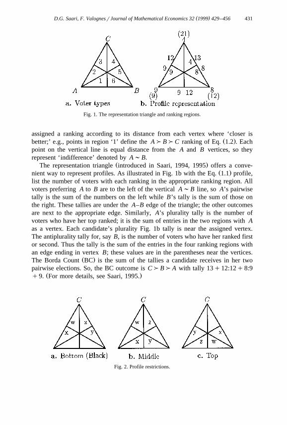
Fig. 1. The representation triangle and ranking regions.

assigned a ranking according to its distance from each vertex where ‘closer isŽ .better;’ e.g., points in region ‘1’ define the A%B%C ranking of Eq. 1.2 . Each

point on the vertical line is equal distance from the A and B vertices, so theyrepresent ‘indifference’ denoted by A;B.

Ž .The representation triangle introduced in Saari, 1994, 1995 offers a conve-Ž .nient way to represent profiles. As illustrated in Fig. 1b with the Eq. 1.1 profile,

list the number of voters with each ranking in the appropriate ranking region. Allvoters preferring A to B are to the left of the vertical A;B line, so A’s pairwisetally is the sum of the numbers on the left while B’s tally is the sum of those onthe right. These tallies are under the A–B edge of the triangle; the other outcomesare next to the appropriate edge. Similarly, A’s plurality tally is the number ofvoters who have her top ranked; it is the sum of entries in the two regions with Aas a vertex. Each candidate’s plurality Fig. 1b tally is near the assigned vertex.The antiplurality tally for, say B, is the number of voters who have her ranked firstor second. Thus the tally is the sum of the entries in the four ranking regions withan edge ending in vertex B; these values are in the parentheses near the vertices.

Ž .The Borda Count BC is the sum of the tallies a candidate receives in her twopairwise elections. So, the BC outcome is C%B%A with tally 13q12:12q8:9

Ž .q9. For more details, see Saari, 1995.

Fig. 2. Profile restrictions.


If n is the number of voters with the jth preference, the total number of votersj6 Ž .is nsÝ n . We use the n rn fraction of voters of each type; e.g., for Eq. 1.1js1 j j

they are 9r21, 8r21, and 4r21.Ž .The profile restrictions are in terms of C; e.g., Black’s condition Fig. 2a is

where C never is bottom ranked, so xsn rn, ysn rn, wsn rn, zsn rn,2 5 3 4

Fig. 2b is where C never is middle-ranked, and Fig. 2c is where C never is topranked. The x, y, z, w definitions, illustrated in the figures, are selected tofacilitate comparisons.

2. Pairwise votes with Black’s restrictions

The definitions of x, y, z, w from Fig. 2a require all terms to be non-negativeand

xqyqzqws1. 2.1Ž .Ž .By using ws1y xqyqz , a profile becomes a point in Fig. 3a tetrahedron

<T s x , y , z x , y , zG0, xqyqzF1 . 2.2� 4Ž . Ž .1

Ž .Thus, T is the profile space for Black’s condition where each rational T point1 1

represents a unique normalized profile. It is easy to convert a normalized profileŽ .into an integer profile; e.g., point 3r20, 7r20, 4r20 gT represents a twenty1

voter profile where 3, 7, 4, and 6 voters have, respectively, preferences of type 2,Ž Ž . .5, 4, and 3. The missing type-3 fraction is ws1y xqyqz s6r20 .

Ž .The almost indistinguishable Fig. 3b represents profiles as x, y, z, w in a fourdimensional space where each unanimity profile defines a unit vector on a

4 Ž .particular R coordinate axis. The vertices are equal distance apart, so Eq. 2.1forces this space to be the Fig. 3b equilateral tetrahedron denoted by ET . In both1

representations, w increases as profile p approaches the rear vertex. T and ET1 1

differ in that the T faces are three right and one equilateral triangles while each1

Fig. 3. Pairwise comparisons in Profile Space.


ET face is an equilateral triangle. As a linear transformation converts one1

tetrahedron into the other, statements about the geometric properties and probabili-ties of events remain the same.

2.1. Pairwise Õotes

� 4As shown in Fig. 2a, B beats A in the A, B pairwise vote if and only ifyqz)1r2. Thus, the A;B plane yqzs1r2 divides T into two sets1

determining who beats whom; it is the slanted plane in Fig. 3. Because ys1ensures that B%A, the side with the y vertex supports B%A outcomes. TheA;C and B;C divisions correspond, respectively, to xs1r2 and ys1r2planes—the vertical planes in Fig. 3. As it is easy to determine which rankings are

Ž .on each side of an indifference plane by computing what happens at a vertex , wehave identified all profiles which define each possible pairwise outcome. The four

Ž .strict outcomes are denoted by Eq. 1.2 numbers.Ž .Let s interchange A and B in a ranking and let s p be the profile created

Ž .from p by interchanging A and B for each voter. If f p is the election ranking,then neutrality requires

f s p ss f p . 2.3Ž . Ž . Ž .Ž . Ž .Ž .The importance of Eq. 2.3 for our purposes is the following.

Ž .Proposition 1. If p satisfies Black’s condition, then so does s p .

Ž .The Fig. 3 symmetry reflects Proposition 1; e.g., if p elects A, s p elects B;Ž .if p has C winning with A in second plate, s p has C winning with B in1 1

second place. To demonstrate how conclusions follow from Fig. 3, we find theŽ .likelihood of each pairwise election outcome. If F x, y, z, w is the probability

Ž .distribution, then P j , the probability of outcome j, js2, 3, 4, 5, is

P j s F x , y , z , w d x d y dw d z 2.4Ž . Ž . Ž .HHHHR j

where R is the Fig. 3 region defining a type j outcome. So, if each Fig. 3 profilejŽ . Žis equally likely F is a constant , elementary geometry used to compute the ratio

. Ž . Ž .of volumes of the different regions and of T shows that P 2 sP 5 s1r81Ž . Ž .while P 3 sP 4 s3r8. More generally, for any centrally distributed probabil-

ity distribution, where the distribution uses the number of voters of each type butŽ Ž ..not the type names, the s symmetry of the figure about 1r4, 1r4, 1r4

Ž . Ž . Ž . Ž .ensures that P 2 sP 5 , P 3 sP 4 . If the probability emphasizes the centralŽ . Ž . Ž .point 1r4, 1r4, 1r4 , such as the central limit theorem, the P 3 sP 4

Ž . Ž .likelihood increases at the expense of P 2 sP 5 . These new, useful resultsfollow immediately from the T geometry.1


Theorem 1. With Black single peakedness condition where each T profile is1

equally likely,

1 3P 2 sP 5 s , P 3 sP 4 s . 2.5Ž . Ž . Ž . Ž . Ž .

8 8

Ž .With n Õoters, as n™` the Eq. 2.5 Õalues are limits approached at leastwith order ny 1. This limit also holds for the setting where the number of Õoters isbounded by n.

The probability of a type 2 or 5 outcome for precisely n odd or eÕen Õoters is,respectiÕely,

1 3 1 1 3 11q ™ and 1y ™ . 2.6Ž .

8 nq2 8 8 n nq4 8Ž .

If the number of Õoters is less than or equal to n, the two respectiÕeprobabilities are

21 n q7nq16 nq7 1 1 nq4 nq1 1Ž . Ž . Ž . Ž .™ and ™ 2.7Ž .228 8 8 8n q5nq10n q5nq10 nq5Ž . Ž .

The probability of a type 3 or 4 outcome for precisely n odd or eÕen Õoters is,respectiÕely,

3 1 3 3 4nq3 31y ™ and 1y ™ . 2.8Ž .

8 nq2 8 8 nq1 nq3 8Ž . Ž .

The respectiÕe Õalues if the number of Õoters is less than or equal to n are

3 23 n q 26r3 n q25nq 88r3 3Ž . Ž .™28 8n q5nq10 nq5Ž . Ž .

23 n q 11r3 nq 4r3 nq1 3Ž . Ž . Ž .Ž .and ™ .28 8n q5nq10 nq5Ž . Ž .

So, it is more likely to have a strict outcome with an odd than with an evennumber of voters. The following illustrates this oddity for a type 3 outcome by

Ž .computing the 3r8 multiples of Eq. 2.8 . The oscillations, showing the rapid andslower approaches to unity for odd and even n values, capture the impossibility ofa tie with an odd number of voters; odd values of n have no boundary points.


The probabilities described later in this paper are computed as in the following,so only the limiting values are given hereafter. This proof proves that these limitsare approached at least with order ny1 as n™`; it manifests the distribution ofrational points in T and ET .1 1

Proof. The limiting values follow from the geometry. The probabilities for n usethe equalities

k kk kq1 1Ž .kq1 2js s , j s k kq1 2kq1 ,Ž . Ž .Ý Ýž /2 2 6js1 js1

2kkq13j s 2.9Ž .Ý ž /2

js1

ŽTo compute the number of T points with n voters, if wsarn a of the n1. Ž .voters have type 3 preferences , then xs nya rn requires yszs0—there is

Ž .one point. Similarly, the number of points with xs nyay j rn is the numberof ways a y numerator can be selected with denominator n and yqzs1yxyw

w Ž .xs jrn; this is jq1. Continue until xs0s nyay nya rn which is sup-Ž .ported by nya q1 points. Thus the total number of points is

n nyaq1 n nyaq1 nyaq2 nq1 nq2 nq3Ž . Ž . Ž . Ž . Ž .js s .Ý Ý Ý

2 6as0 js1 as0

2.10Ž .

The number of T points with common denominator less than or equal to n is1

n1 12kq1 kq2 kq3 s n q5nq10 nq5 n . 2.11Ž . Ž . Ž . Ž . Ž . Ž .Ý

6 24ks1

ŽWhen n is odd, the number of points satisfying wsarn and xs nyay. Ž .j rn again is jq1. The difference in the computation from Eq. 2.10 is that

Ž . wŽcondition x)1r2 restricts the computations to xs nq1 r2n, or until js n. xy1 r2 ya . Thus the summation is

Ž . Ž .ny1 r2 nq1 r2ya 1js nq1 nq3 nq5 .Ž . Ž . Ž .Ý Ý

48as0 js1

Ž . Ž .Eq. 2.6 follows by dividing this value by that of Eq. 2.10 . To find theprobability value for all fractions satisfying x)1r2 with common denominatorkFn, we compute

n1 12kq1 kq3 kq5 s n q7nq16 nq7 n ,Ž . Ž . Ž . Ž . Ž .Ý

48 8 24Ž .ks1

Ž .which leads to the first of the Eq. 2.7 expressions.


For a the type 3 outcome, a fixed x restricts the admissible y, z values to awŽ . x Ž .right triangle; when ys ny1 r2n y jrn , there are jq1 admissible z

Žnq1.r2 wŽnumerators. So, when n is odd, each x value is associated with Ý js nqjs1.Ž .x Ž .1 nq3 r8 points. As x ranges from xs0rn to xs ny1 r2n, there areŽ . wŽ .2Ž .xnq1 r2 x values leading to nq1 nq3 r16 points. The result follows.The remaining expressions are similarly obtained. I

2.2. Other pairwise properties

To see how geometry dictates properties of procedures, observe that each set isŽ .convex. For any two points in a region, the connecting line also is in the region.

To see the significance, suppose two subcommittees with six and 24 voters haveŽ . Ž . Ž .respective preferences p s x, y, z s 3r6, 2r6, 0 so ws1r6 and p s1 2

Ž . Ž .12r24, 0, 8r24 so ws4r24 . The normalized profile defined by combiningŽ . Ž Ž ..the committees is p s 15r30, 2r30, 8r30 s1r5 p q 1y 1r5 p ; ws3 1 2

5r30. More generally, if m is the number of voters in profile p , js1, 2, thej j

normalized form the combined profile ism1

p smp q 1ym p ; ms . 2.12Ž . Ž .3 1 2 m qm1 2

Ž .According to Eq. 2.12 the normalized combined profile is on the lineconnecting the two original profiles. So, if p and p define the same outcome,1 2

this common outcome holds for the combined profile p . Conversely, if a profile3

region is not convex, examples exist where p and p define a common outcome1 2

different from p . Implications arise by postulating conditions where the same3

outcome should persist when profiles are combined; this includes monotonicityand the following.

² : � 4Definition 1. An agenda A, B, C is where the winner of A, B majorityelection is advanced to be compared with C. A procedure is weakly consistentŽ .Saari, 1995 if when p and p have the same outcome, that is the p outcome.1 2 3

Ž .Positive involvement Saari, 1995 is where if c wins with p , and if p is aj 1 2

profile of the same type of new voters where c is top-ranked, then c still winsj j

with p .3

An agenda does not satisfy weak consistency or positive involvement, so itsuffers the ‘no-show’ paradox from Moulin, 1988 where by not Õoting, a voter

Ž .forces a better outcome. Also see Fishburn and Brams, 1983. The convexityensured by Black’s condition, however, permits both conditions to hold.

Theorem 2. In general, an agenda does not satisfy positiÕe inÕolÕement and weakconsistency. With Black’s single peakedness condition, howeÕer, an agenda satis-fies both conditions.


² :Proof. A wins with A, B, C iff p is in region 2; B wins iff p is in region 5; Cwins iff p is in the 3, 4 region. As all sets are convex, the conclusion follows SaariŽ .1995 . I

2.3. Strategic behaÕior

As the Gibbard, 1973, Satterthwaite, 1975 Theorem requires all three candi-Ž .dates non-dictatorial procedures to admit situations where some voter can

successfully manipulate the system, an agenda can be manipulated. But does theGibbard–Satterthwaite Theorem hold for agendas when Black’s condition issatisfied? To be a meaningful, both the sincere and strategic profiles must satisfyBlack’s condition; i.e., strategic voters choose strategies which satisfy Black’scondition with respect to C.

Theorem 3. With Black’s single peakedness, there neÕer is a situation where aÕoter, by choosing a strategy consistent with Black’s restraint, can successfullymanipulate the outcome of an agenda.

Proof. Let p and p be, respectively, the sincere and the strategic profile; to1 2Žchange the outcome, p must be in a different profile set. This requires Chap. 5,2

.Saari, 1995 the profile change vsp yp to cross a Fig. 3 indifference2 1

boundary. To explain v, if a type 2 voter votes like type 5, x decreases and yŽ .Ž .increases by 1rn to define vsd s 1rn y1, 1, 0 in the direction from the2 ™ 5

Ž .x to the y vertex. Similarly, because ws1y xqyqz , a change from type 3Ž .Ž .to type 4 defines d s 1rn 0, 0, 1 in the direction from the w to the z3™ 4

vertex. Since each voter type has three options, Black’s condition define 12strategies—the 12 directions from one vertex to another. Six follow; the others usethe relationship d syd ; e.g., a type 5 voter voting as though type 2j™ k k ™ j

Ž .Ž .defines d syd s 1rn 1, y1, 0 .5™ 2 2 ™ 5

Ž .2.13

For a manipulation to be successful, the new outcome must be preferred by thestrategic voter. With Black’s condition, only the xs1r2, ys1r2 boundariesseparate agenda winners. With Fig. 3, we can determine which d vectors crossj™ k


Žthe boundaries and where this improves the voter’s outcome. So the geometry.identifies who can manipulate and when. For instance, a vector crosses the

xs1r2 boundary iff the x component of d is nonzero where the signj™ k

determines the direction of change. For instance, if a type 2 voter votes as type 5,Ž .the nd s y1, 1, 0 change can cross the xs1r2 boundary. But, the sincere2 ™ 5

p must be on the x)1r2 side; e.g., p elects A. As the new C outcome changes1 1

the type 2 voter’s top-ranked alternative to his second one, this move is counter-productive. A similar analysis using all d with the boundaries proves thej™ k

theorem. I

For any procedure depending on pairwise voting, issues including strategicaction, monotonicity, etc., can similarly be analyzed with Fig. 3. The resolution of

Žthese issues, however, now is possible and easy because of the geometry see.Saari, 1995 .

3. Positional voting with Black’s condition

Positional voting assigns w points to a voter’s jth ranked candidate, w Gwj 1 2

Gw s0, and ranks the candidates according to the sum of assigned points. A3

normalization assigns one point to a voter’s first choice to define the Õoting ÕectorŽ .w s 1, l, 0 , 0FlF1; e.g., the normalized version of the system where 7, 2,l

Ž .and 0 points are assigned to candidates is w s 7r7, 2r7, 0 . Important2r7Ž . Ž .systems are the plurality w s 1, 0, 0 , BC w s 1, 1r2, 0 , and antiplurality0 1r2

Ž .w s 1, 1, 0 votes.1

To find A’s w tally from Fig. 1a, she receives one point from voters who havel

Ž .her top ranked the number of voters in regions 1 and 2 and l points from votersŽ .who have her second ranked the number of the voters in regions 3 and 6 . For

ŽBlack’s Fig. 2a condition, A’s tally is xqwl. Each candidate’s tally after the.ws1yxyyyz substitution is given next.

Ž .3.1

3.1. Geometry of w outcomesl

To analyze w , mimic the approach for pairwise elections. Namely, to find thel

� 4w relative ranking of the pair A, B , set their tallies equal to find that the A;Bl

Ž . Ž .plane is xyy ql 1yxyyy2 z s0; this plane divides T into profile sets1


with relative A%B and B%A w rankings. For each l, the equation is satisfiedl

Ž .by the line t, t, 1r2y t , y`- t-`, so the A;B w planes rotate about thisl

line—the rotation axis—with l changes. A plane is determined by a line andanother point, so each w plane is determined by the rotation axis and where itl

intersects the y-axis. The information for all pairs follows.

Ž .3.2

To appreciate how the rotating planes affect election outcomes, notice when aplane passes over a profile, the election ranking changes. All conflict is caused bythis rotation effect. As each indifference plane has a different rotation axis, radicalchanges in election rankings must occur with changes in l; i.e., a wide selectionof profiles change election outcomes with different w as apparent from Fig. 4l

Ž . Ž . Ž .which depicts the plurality ls0 , BC ls1r2 , and antiplurality ls1behavior.

ŽThe ls0 equations for the A;B, A;C, B;C planes respectively, ysx,.ys1y2 x, 2 ys1yx , depend only on x and y values, so the plurality figure

depicts where they meet the xyy coordinate plane; the actual planes extendvertically in the z direction. The respective equations of these planes for ls1 areyqzs1r2, yqzs0, yqzs1, so only the antiplurality A;B plane passes

Žthrough the T interior. The A;C plane is the x-axis, the B;C plane is the1.slanted T boundary line in the xs0 plane. By being the ‘middle’ transition1

stage, the Borda planes, xy3 yy2 zsy1, zs2 xy1, xq3 yqzs2, involveall three variables.

The dotted Fig. 3 lines represent ranking regions of pairwise outcomes. Thus, pon one side of the pairwise plane for a particular pair and on the other for a l

Fig. 4. Positional comparisons.


plane generates conflicting outcomes. The significant difference in these planesensures wide spread differences in outcomes. The BC planes, however, more

Žclosely approximate the dotted pairwise planes; this supports the fact e.g., Saari,.1997a,b that BC outcomes most closely reflect the associated pairwise outcomes.

The rotation of planes from the ls0 position to the ls1 final locationidentifies new results; e.g., we determine how likely it is for p to retain the same

Žranking with the pairwise and all w methods. From the figures, this compatibilityl

.occurs only with type 3 and 4 outcomes. Also, we determine the likelihood theseŽprocedures have the same candidate top-ranked. The answer involves the volume

.of the region with a type 3 or 4 outcome for all methods.

Theorem 4. If all profiles in T are equally likely, the probability that a profile1

has the same ranking with the pairwise and all w is 1r9. Thus, 8r9 of thel

profiles change rankings with procedure. The likelihood that the same candidate istop-ranked with any of these procedures is 11r18f0.611.

Proof. The region where all procedures have a type-3 ranking is bounded aboveŽ .by the ysz plane the profiles giving a relative A;B antiplurality ranking and

the region in the x–y plane defined by the type-3 plurality outcome. This volumeis

Ž .1r3 1yy r2 1y d x d ys .H H

108y0

By s symmetry, the region for a type-4 outcome has the same volume. Therefore,the probability is determined by doubling this common value and dividing by 1r6Ž .the volume of T .1

Similarly, the antiplurality outcomes ensure that if the same candidate iselected, she is C. To find the likelihood, double the volume of the region whichhas both a type-3 plurality and pairwise outcome and divide by 1r6. The volumeis

Ž .1r3 1yy r2 11w x1yxyy d x d ys .H H

216y0

I

Ž .As most about 88.9% profiles change rankings, it may appear that Black’scondition does not provide much assistance. Black’s condition, however, ensuresthe same ‘winner’ for over 60% of the profiles. When compared with Merlin etal., 1997 where they find that with no restrictions, this ‘common winner’phenomenon occurs with slightly over half of the profiles, it follows that Black’scondition does provide some relief.

The advantages offered by Black’s condition come from the A–B symmetry ofŽ .Fig. 4 used to prove Theorem 4 . This s symmetry reflects Proposition 1 and the


Ž .neutrality of positional methods. Namely, if f p, w is the w ranking for profilel l

p, then

f s p , w ss f p ,w 3.3Ž . Ž . Ž .Ž . Ž .l l

Ž .That is, for each p, s p satisfies Black’s condition and defines the w outcomel

which reverses A and B. So, the likelihood a procedure has a type-3 outcomeequals the likelihood it has a type-4 outcome. This is true for any probabilitydistribution which respects the s symmetry.

3.2. Plurality and pairwise conflicts

The ls0 portion of Fig. 4 displays considerable conflict between the pairwiseand plurality outcomes. For instance, the profile line defining an A;B;C

Žplurality outcome extending vertically from where the three solid lines cross in.the ls0 figure is in the interior of the sets of pairwise outcomes with C

top-ranked. But profiles supporting any desired plurality election abut this line, soany of the 13 plurality rankings can accompany a pairwise ranking where C is topranked. In the two regions where the pairwise outcomes have C middle-ranked,the plurality ranking either agrees with the pairwise outcomes, or it relegates C tolast place. The geometry also proves that all discrepancies are robust.

Particularly troubling conflicts are the reversed plurality and pairwise rankings;Ž . Že.g., the Eq. 1.1 profile. But as this occurs in the smallest Fig. 4 regions e.g., a

Ž . .type 3 pairwise C%A%B and the reversed type 6 plurality rankings , thisperverse event is the least likely to occur. Indeed, the volumes of the T region1

with a type 3 pairwise outcome is 1r16 and that of the ‘type 3 pairwise outcomeŽ .and type 6 plurality’ region is 1r 54=16 . Consequently, the likelihood the

plurality ranking reÕerses a giÕen pairwise ranking where C is the Condorcetwinner is 1r54f0.0185. Assuming all T profiles are equally likely, Black’s1

condition allows only about 2% of the elections to experience this perversebehavior. It also follows from the geometry that this behavior requires at least 12voters.

Theorem 5. With Black’s condition, assume that all T profiles are equally likely.1

If C is the Condorcet winner, the likelihood a plurality ranking completelyreÕerses the pairwise ranking is 1r54f0.0185. Any such profile inÕolÕes at leasttwelÕe Õoters; one example has fiÕe Õoters with preferences A%C%B, four withBAC%A, and three with C%B%A.

If C is the Condorcet winner, the likelihood C is plurality bottom, middle, andtop ranked are, respectiÕely, 0.0648, 0.1204, 0.8148.

� 4 � 4Proof. By integration, the volume of the type 3 pairwise l type 6 pluralityregion is

y1r2 1 1yy d x d ys . 3.4Ž .H H ž /Ž . 2 54=161r3 1yy r2


The conditional probability assertion follows from the 1r16 volume of a profile�set with type 3 pairwise ranking. As a similar statement holds for the type 4

4 � 4pairwise l type 1 plurality region, the assertion follows by combining probabili-ties.

A p with the minimum number of voters illustrating a specified behavior is a�point in the T region with the smallest common denominator. To find pg type 41

4 � 4pairwise l type 1 plurality , the pairwise outcomes require yqz)1r2, y-1r2Ž Ž .. Ž . Žwhile the plurality requires Eq. 3.2 x)y so A%B and 1-xq2 y so

.B%C . Expressing fractions as xsXrd, ysYrd, zsZrd, with integers, wehave

2 YqZ )d , 2Y-d , X)Y , d-Xq2Y and XqYqZFd.Ž .Ž .The X)Y or Xy1GY and d-Xq2Y conditions require d-3 Xy2, or

Ž .dq2 r3-X. So, for ds10, 11, 12, it follows that XG5. The other equationsprove that no example exists for dF11; a ds12 example is the indicated profile.

I

While Theorem 5 shows that consistency between the pairwise and pluralitywinners occurs about 81% of the time, it carries the troubling message that evenBlack’s condition permits conflict in about one out of five plurality elections. Butthe conflict between the pairwise and plurality outcomes is, in general, more

Ž .severe Merlin et al., 1997; Saari and Tataru, 1999 , so Black’s condition reducesthe likelihood of its occurrence. Also, compare the simplicity of our approach withthat used by these papers and, say, Gehrlein, 1981 and Lepelley, 1993.

3.3. Different l’s

Ž .Fig. 4 shows that Black’s condition restricts the antiplurality ls1 strictoutcomes to C%B%A or C%A%B where each has the same limiting 1r2probability. The only conflict with pairwise rankings, which interchange theantiplurality’s two top ranked candidates, occurs with probability 1r4. All otherw outcomes depend on how the indifference planes change; e.g., the A;Bl

Ž . Ž .l-plane rotates about the line connecting 0, 0, 1r2 with 1r2, 1r2, 0 —the lineconnecting the midpoint on the z-axis with the midpoint of the line in the x–yplane. The monotonic progress of this plane is captured by the movement of itsy-axis intercept which starts at the origin when ls0 and moves monotonically to

Ž .ys1r2 when ls1. So Fig. 4 , the A;B plane tilts from its initial verticalposition until it reaches its final ls1 orientation parallel to the x-axis. The

Ž . Ž .B;C plane rotates about the line connecting 1, 0, 1 and 0, 1r2, 1r2 ; theŽ .y-axis point monotonically moves from ys1r2 ls0 to ys1 when ls1

Ž .where Fig. 4 it is parallel to the x-axis. The more dramatic A;C plane motionŽ . Ž .rotates about the axis defined by 1r2, 0, 0 and 0, 1, y1 , but its y-axis point

moves rapidly. At ls0, it is at ys1, but as l™1r2, it moves to infinity


Ž .at the BC the plane is parallel to the y-axis , to re-emerge from negative infinitywhen l)1r2 to approach zero as l™1.

Theorem 6. With Black’s single peakedness, if C is the Condorcet winner andeach profile in T is equally likely, then the likelihood C is w bottom ranked1 l

monotonically decreases from 0.0648 for the plurality Õote to zero as l™1r2.For lG1r2, C neÕer is bottom ranked. The likelihood C is w second rankedl

monotonically decreases from 0.1204 for the plurality Õote to zero as l™1. Thelikelihood that C is w top ranked monotonically increases from 0.8148 for thel

plurality Õote to unity as l™1. Only the antiplurality Õote always has C topranked with Black’s conditions.

3.4. Runoff elections

Other geometric consequences of Fig. 4 are illustrated with w runoff electionsl

where the two w top-ranked candidates advance to a runoff to determine thel

‘winner.’ For a candidate to win, the profile must be in a T region where she is at1

least second ranked and wins the associated two candidate election. The geometryof this profile set provides new results.

Theorem 7. With Black’s condition, a w runoff satisfies positiÕe inÕolÕement andl

weak consistency with respect to A and B. Weak consistency holds for C if andonly if lG1r2.

For a w runoff election where l-1r2, there exist situations where each ofl

two committees elect C, but when they combine as a full group, the sincereoutcome is A.

� 4 � 4Proof. A wins only if pg type 2 pairwise l type 1, 2, or 3 w region. In Fig.l

4, p is in the portion of the small tetrahedron with vertex xs1 defined by theŽ .dotted lines type 2 pairwise outcome with a type 1, 2, or 3 w outcome. It isl

Ž .clear from Fig. 4 and the interpolation for other l that this region is convex for�any l. A similar assertion holds for B. However C wins if pg type 3 or 4

4 � 4pairwise and w has anything other than a type 1 or 6 outcome . For l-1r2,l

this exclusion of w outcomes creates a dent in the profile region that deniesl

convexity and forbids ‘weak consistency.’ The more forgiving ‘positive involve-Ž . Ž . Žment’ Saari, 1995 restricts p to either the w all voters are type 3 or z all2

.voters are type 4 vertices. It is obvious from the geometry that if p elects C with1

this runoff, the line connecting p with either p choice remains in the region.1 2

Examples exploit the lack of convexity of the region where C is elected; i.e., p1

is in a type 2 w region near the B;C w plane where C is the Condorcetl l

Ž .winner. To illustrate with ls0, the profile x, y, z must satisfy x-1r2,Ž . Ž .xq2 y-1, 2 xqy)1; e.g., x, y, z s 9r20, 5r20, 0 . Select p in the region2


Želecting C with a type 5 w outcome near the A;C boundary; e.g., 5r20,l

. Ž .9r20, 0 . Use Eq. 2.12 to select the committee sizes so that p , the full3

committee, elects whomever we choose. For ls0, a choice to elect A has 3r5 ofall voters in the p subcommittee. Thus p has 27 of type 2, 15 of type 5, and 181 1

of type 3 while p has 10 of type 5, 18 of type 5, and 12 of type 3.2 I

3.5. Strategic behaÕior

The manipulative behavior of w elections and runoffs is determined by thel

Ž .geometry of boundaries. To use the scalar product approach of Saari 1995 , thegradients of the A;B, C;A, C;B planes for w are, respectively,l

1yl, y1yl, y2l , y2q2l, y1q2l, l ,Ž . Ž .and y1ql, y2ql, yl .Ž .

ŽEach gradient points in the profile direction helping the first listed candidate. Thefirst vector supports A over B; the other two directions support C over the ‘other’

.candidate. To determine the effects of a strategic action, compute the scalarproduct of each gradient with each d ; positive or negative values mean,j™ k

Žrespectively, that the change helps or hurts the indicated candidate either A or.C ; a zero value means the change has no impact. The values follow.

Ž .3.5

So, if a type 2 voter uses d or d , the outcome is personally worse2 ™ 5 2 ™ 4

because the change counters the voter’s true preferences. For instance, the positivevalue for d helps C over the voter’s top choice of A; the two negative values2 ™ 5

indicate strategies that help his lower ranked candidate at the expense of a higherranked one. The only strategic action is if l-1 where the voter uses d to2 ™ 3

assist C over B; the sincere p must be near the B;C plane with a w type 1 or1 l

5 outcome. According to Fig. 4, a type 1 outcome requires l-1r2. A similaranalysis determines when each type of voter can successfully manipulate theoutcome.

Theorem 8. With Black’s single peakedness condition, a type 2 agent cansuccessfully Õote strategically only by Õoting like a type 3 Õoter with w , forl

l-1, when the sincere w outcome has B narrowly ahead of C. Similarly, thel


only time a type 5 agent can successfully Õote strategically by Õoting like a type 4agent is when the sincere w outcome, l-1, has C narrowly ahead of B.l

A type 3 Õoter can Õote as though a type 2 Õoter for a better w outcome,l

l-1, when the sincere outcome has B narrowly ahead of A. This Õoter can Õote( ) ( )either as though type 4 for 0-l-1 or as though type 5 for 1r2-l when

the sincere w outcome has A narrowly ahead of C.l

A type 4 Õoter Õoting as a type 5 Õoter can haÕe a better w outcome, l-1,l

when the sincere w outcome has A narrowly ahead of B. This Õoter can Õotel

( ) ( )either as though type 3 for 0-l-1 or as though type 2 for 1r2-l whenthe sincere w outcome has B narrowly ahead of C.l

Proof. A d profile change crosses a particular boundary when the sign of thej™ kŽ .appropriate Eq. 3.5 entry is non-zero. Values of ‘y1q2l’ change direction

Ždepending upon whether l is larger or smaller than 1r2. As the change occurswith the BC, the associated zero value means that the BC has no strategic

Ž .advantage; this is compatible with the general result Saari, 1995 that the BCminimizes the likelihood of a successful manipulation by a small number of

. Ž .voters. The sign of a Eq. 3.5 entry gives the directional change, so, to alter theelection outcome, p must be on the appropriate side of the boundary. The last1

step involves determining whether a change in a pairwise ranking is compatible, orcontrary, to the strategic voter’s sincere preferences. I

The more complicated strategic analysis of w runoffs requires determiningl

which two candidates are w top ranked as they are advanced to the runoff andl

then the runoff outcomes.

Theorem 9. EÕen with profiles satisfying Black’s single peakedness conditionwhere a strategic Õoter must Õote consistent with this constraint, there existsituations where a Õoter can obtain a personally better outcome by Õotingstrategically in a w runoff election when l-1r2. But, Black’s condition makesl

it impossible for a Õoter to successfully manipulate the w runoff when lG1r2.l

Ž .Proof. From Eq. 3.5 , when a type 2 voter votes as type 3, the outcome crossesthe B;C w surface if l-1 and if p is near the B;C plane with a type 5 or 1l 1

w outcome. The first case only interchanges whether B or C is top ranked, so itl

does not change the candidates in a runoff and has no effect on the outcome.Ž .According to Fig. 4 the second setting sincere type 1 outcome prohibits B from

advancing to the runoff only if l-1r2. As this strategic action advances A andC, rather than A and B to the runoff, the final outcome depends upon the pairwiseelections. If p has a type 2 pairwise outcome, the strategic action has no1

effect—A wins with or without the strategic action. If p is in the region with type1

3 pairwise outcomes, C wins by beating A. But the sincere vote has A beating B,


so the strategic vote is counterproductive for the type 2 voter. The remainingpossibility is if p is in a region of type 4 pairwise outcomes; here C beats A1

whereas the sincere vote has B beating A. Thus, in a narrowly defined T region1Žwhich exists for l-1r2, a type 2 voter can be strategically successful. With a

slight miscalculation of the pairwise outcomes, the strategy can be counterproduc-. Ž .tive. All remaining strategic actions follow similarly from Eq. 3.5 and Fig. 4.

To see why a strategic voter cannot successfully manipulate a w runoff methodl

for lG1r2, notice that the limited number of w outcomes allow a changel

between a type 3 and 4 outcome to alter which candidates are in the runoff.However, these locations for the sincere profile also are where C wins all pairwiseelections. Thus, the strategic action does not alter the outcome. I

3.6. Line of indifference

A slight change in an A;B;C outcome creates any other ranking, so subtlew behavior is detected by determining how the ‘completely tied’ w outcomesl l

change with l. To find this w point, solve the A;B;C equations to obtainl

x , y , zŽ .1ql 1y3w 1q l2 yl 1y3w 1y3w ql 3wy2Ž . Ž . Ž . Ž . Ž .

s , , .ž /3 3 1yl 3 1ylŽ . Ž .3.6Ž .

w Ž .xAn equivalent expression using xs 1ql 1y3w r3 is

1y2wq3 wy1 xq3 x 2 1y2 x 2 q3w xy1qwŽ . Ž .x , y , z s x , ,Ž . ž /2y3 xqw 2y3 xqwŽ . Ž .

3.7Ž .w Ž . .where xg 1r3, 2y3w r3 . The solutions decrease from a T line segment1

Ž . Ž1r3, 1r3, 1r3yw ; 0FwF1r3, for the plurality vote to the T point 1r2,1. Ž Ž ..1r2, 0 for the BC. It leaÕes T for l)1r2 to approach infinity Eq. 3.6 as1

l™1; this causes the Fig. 4 antiplurality properties. This geometry discloses asurprisingly wide variety of election conflicts allowed by Black’s condition.

Theorem 10. With Black’s condition, for any integer k between one and seÕen,there exist p with precisely k w election rankings as l Õaries. Indeed, for somel

p, each candidate wins with an appropriate w , while other p require eachl

candidate to be bottom ranked with an appropriate w .l

If all profiles in T are equally likely and C is the Condorcet winner, the1

probability p has seÕen different w outcomes where each candidate wins withl

some w is no more than 0.0062. Any example requires at least 19 Õoters; onel

such example is where 8 haÕe A%C%B, 7 haÕe B%C%A, and 4 haÕeC%B%A.


Fig. 5. ET curves of completely tied outcomes.1

The probability p has seÕen different w outcomes where each candidate losesl

with some w is at least 0.0586. An example requires at least seÕen Õoters; onel

such example is where 4 haÕe A%C%B, 3 haÕe B%C%A, and 3 haÕeC%B%A.

Ž Ž . Ž ..Proof. Profiles supporting a w complete tie Eqs. 3.6 and 3.7 define a line, sol

it suffices to locate the end points. Fig. 5 displays the curve of endpoints on thews0 and zs0 ET faces.Each l defines a point on each curve equal distance1

from the ls0 point. Each curve leaves its face at the BC point. For each l, theprofiles causing a w complete tie is the line connecting the indicated l points onl

the two faces. The Fig. 5 faces are subdivided into plurality ranking regions; i.e.,the line of A;B;C plurality outcomes connects the two center points and the

Ž .BC point is where the curves leave the edge at 1r2, 1r2, 0 . The faces areŽ .similar after reversing directions because Black’s condition is invariant with s

Ž Ž ..Proposition 1, Eq. 3.3 . Indeed, the s symmetry requires the w A;B;Cl

line to pass through the A;B plurality plane when zsw.To explain the narrow region between the curve and A;B plurality line, Fig.Ž .6 an enlarged ws0 face has dashed lines where w has tied pairs; the lines1r4

Fig. 6. ET curve of completely tied outcomes.1


intersect on the curve where w has the A;B;C outcome. The Fig. 61r4Žnumbers identify which profiles define the six w strict election rankings. A1r4

.symmetric picture holds for the zs0 face. By differing from plurality lines, thedashed lines define profiles with different plurality and w outcomes. As a p1r4

with a w A;B;C outcome is in the interior of the type 1 plurality set, slight1r4

changes in p change the w outcome to any of 13 three-candidate rankings whilel

the A%B%C plurality outcome remains. This conflict allowed by Black’scondition is more serious than suggested by the introductory example.

� 4 � 4Now consider a pg type 1 plurality l type 4 w region as l varies from1r4

0 to 1r4. Each l defines dashed lines similar to Fig. 6, so as l varies p’s strictelection rankings vary from type 1 to 6 to 5 to 4 allowing each candidate to ‘win’with an appropriate w ; with ties, p admits seÕen different election rankings.l

Moreover, these properties hold for all p between the curve and the A;Bplurality line. In the zs0 face, the plurality ranking is type 6 and the wl

outcomes range from type 6 to 1 to 2 to 3, so the same properties hold withŽ .changed type numbers required by s . More generally, the set of p with these

properties is defined by the plane of A;B plurality outcomes and the curvedsurface obtained by connecting l points on the curves in each face.

A p in the type 1 plurality region of the ws0 face outside the curve has sevenw election outcomes as l varies, but each candidate loses with some w ratherl l

than wins. Similarly, p in the plurality type 2 region has five w outcomes, p inl

the plurality A%B%C region has six rankings, etc. In the ws0 face, only p inthe plurality type 4 region have a fixed election outcome for all l; in the zs0face, all p with a fixed outcome are in the type 3 plurality region.

Finding a p with the minimum number of voters requires finding a point withthe smallest common denominator in the indicated region. The cone shape

Ž .geometry e.g., Fig. 5 of these regions requires p to be where z or w equals zero;Žlet ws0. If each candidate can win, the w rankings move from type 1 to 6 seel

.Fig. 6 ; e.g., if p has an A;B w ranking, the ranking is A;B%C. Withl

Ž Ž ..integer profiles, the w tally is X, YqlZ, Zql XqY , so an A;B relativel

ranking occurs when

XyYU

l s . 3.8Ž .Z

Because the wU ranking is A;B%C, we have thatl

X)ZqlU XqY , 3.9Ž . Ž .

Ž .or, by substituting the value from Eq. 3.8 ,

Z XyZ ) XyY XqY 3.10Ž . Ž . Ž . Ž .Ž .Eq. 3.10 requires examples with small numbers of voters to have ZfXr2

and XyYs1. So, start with small X and Y values, and determine whetherŽ .ZfXr2 satisfies Eq. 3.10 . If Xs7, Ys6, and Zs3 or 4, the left-hand side of


Ž . ŽEq. 3.10 is 12 while the right is 13, so an example with Xs7 and smaller X.values does not exist. The next choice of Xs8, Ys7, Zs4 works; this is the

example stated in the theorem. Thus, the smallest number of voters is XqYqZs19.

Ž .The difference in constructing p ws0 where each candidate loses with someŽw is that A;B mandates a C%A;B ranking. Fig. 6 requires the rankings tol

. Ž . Ž .go from types 1 to 2 to 3 to 4. So, Eq. 3.8 remains in effect, but Eq. 3.9 isU Ž .reversed to X-Zql XqY to define

Z XyZ - XyY XqY . 3.11Ž . Ž . Ž . Ž .Here, the inequalities are satisfied with small Z values. As the plurality andantiplurality outcomes are, respectively, A%B%C and C%B%A, we haveX)Y)Z, XqYqZ)YqZ)X, or

ZqY)X)Y)Z. 3.12Ž .Thus the smallest Z value is Zs2 when XyYs1, so the smallest example

Ž . Ž .satisfying Eqs. 3.12 and 3.11 is Xs4, Ys3, Zs2. A direct computationshows that C is the Condorcet winner.

To prove the probability statements compute the volume of the region betweenthe curved surface and the A;B plurality plane. To bound this value, notice thatif the curve for the zs0 portion of Fig. 5 is a direct replica of the ws0, ratherthan a reversal, the ratio of volumes of the region and the tetrahedron is less than

Žthe ratio of areas of that bounded by the curve and the ws0 surface. This region.occurs near the A–B edge of the tetrahedron where the volume is ‘pinched.’ The

Žreversal of these curves creates a cone where the actual relative volume probabil-.ity is less than 1r4 of the relative area of the areas. This area is given by

1 1 1 11r22 xy q d xs y ln 2Ž .H

3 3 3 xy2 12 9Ž .1r3

Ž .Saari and Valognes, 1998 . By considering only profiles in the square defined byŽ .the Condorcet condition with area 1r4 , the limiting probability is four times thisŽ .value, or 1r3y4r9 ln 2 f0.0253. Thus, the probability for our problem is

bounded by 0.0253r4f0.0062. The regions where C is the Condorcet winnerŽ .and the plurality outcome is of type 1 or 6 where C is bottom ranked are divided

into two regions by the surface of completely tied outcomes. According toTheorem 5, the likelihood of this occurring with Black’s condition is 0.0648.Therefore, the likelihood p has seven outcomes where each candidate loses withsome w is no less than 0.0648–0.0062f0.0586.l I

These probability estimates confirm the graphics which suggest it is unlikelyfor Black’s condition to allow each candidate to be a ‘winner;’ it occurs in lessthan 1% of the profiles. On the other hand, the polarizing flavor of the 19 voter

Ž .and all other examples, where one candidate A is strongly favored by a segment


of the population but disapproved of by the rest, is a kind observed in actualŽ Ž .elections; e.g., see examples cited in Saari 1995; Saari and Tataru 1999 . So,

probability estimates can be misleading; by identifying the actual profiles, how-ever, we can determine whether this behavior is more likely due to, say, the gametheoretic maneuvering of the candidates.

4. Top-ranked restrictions

Ž .Surprisingly, all conclusions with the ‘never top-ranked’ constraint Fig. 2cfollow directly from the analysis of Black’s condition. This translation is a direct

Ž .consequence of Eq. 4.1 where r represents the reversal of a ranking; e.g.,Ž . Ž .r A%B%C sC%B%A.Let r p be the profile constructed by reversing each

voter’s ranking in p.

Ž .Proposition 2. Saari, 1994, 1995 For all profiles p and all l , 0FlF1, wehaÕe that

f p ,w sr f r p ,w . 4.1Ž . Ž . Ž .Ž .l 1yl

Ž .To illustrate, the reversal of the Eq. 1.1 profile has 9, 8, 4 voters with therespective rankings of B%C%A, A%C%B, A%B%C. According to Eq.Ž .4.1 , the election rankings of this profile with w , w , w reverse, respec-1 1y2r7 0

Ž .tively, the Eq. 1.1 profile outcomes with w , w , w .0 2r7 1

To convert statements about Black’s condition to the ‘top-ranked’ restriction,Ž . Ž .the x, y, z, w representation in Fig. 2c is the reversal of profile x, y, z, w in

Ž .Fig. 2a. This is one of the three Eq. 4.1 steps, so to translate results from Black’scondition to conclusions about the top-ranked condition, carry out the two steps:Ø Election rankings are reversed. By listing outcomes in terms of ‘type’, this

involves adding or subtracting 3 from each type number for results usingBlack’s condition.

Ø Results concerning w in Black’s condition now hold for w for thel 1yl

top-ranked restriction.These conditions are illustrated with Fig. 7, a converted form of Fig. 6, where

Ž .the solid lines divide the ws0 face into antiplurality rather than pluralityranking regions. In Fig. 6, the dashed lines define w ranking regions; Fig. 7 is1r4

divided into w ranking regions. Figs. 3–6 can be similarly transferred to3r4

identify new properties of the top-ranked profile restriction.The geometry remains the same after re-identifying the regions, so each

assertion about Black’s condition has a reversed conclusion for the top-rankedcondition. For instance, the figure corresponding to Fig. 3 shows that the ‘nevertop ranked constraint’ allows only A and B to win with an agenda. The geometryof agenda profile sets differ but remain convex so an agenda still satisfies positive



Žinvolvement and weak consistency. With positional rankings, the antiplurality not.the plurality method has all 13 rankings with a particular pairwise ranking.

Instead of problems occurring for l-1r2, they occur for l)1r2; only the BCŽ .ls1r2 has reasonable properties in both settings. Reversing Theorem 10, it ismore likely for each candidates to win, rather than lose, with some w .l

5. Never middle-ranked restriction

Black’s condition reflects a natural situation where voters never have a popularcandidate bottom ranked, while the ‘never top-ranked’ condition corresponds tosettings involving an unpopular candidate. The last ‘C never middle-ranked’condition captures a polarized setting where the voters either ‘love or hate C.’This constraint represented by Fig. 2b, has added theoretical interest because if p

Ž . Ž . Ž Ž ..satisfies the middle-ranked conditions, then so do profiles s p , r p , s r p ,Ž Ž ..and r s p . These symmetry conditions determine new election properties.

5.1. Pairwise Õote

All results use the same approach, so only new kinds of assertions aredescribed. From Fig. 2b, the planes of pairwise votes for A;B, A;C, B;C,which are respectively,

1 1 1yqzs , xqys , xqys ,

2 2 2

partition profile space T as in Fig. 8. The two planes divide T into regions with3 3

strict pairwise outcomes of types 1, 3, 4, 6. The vertical plane, xqys1r2,� 4 � 4 � 4serves the A, C and B, C rankings; the slanted plane divides the A, B

rankings. So, C is the Condorcet winner for all profiles on the side of the vertical


Fig. 8. Pairwise comparisons.

plane containing the vertical axis. The profiles sets where A and B are Condorcetwinners are on the other side of this vertical plane; the two regions are determinedby the slanted plane. All regions where a candidate is the Condorcet winner areconvex.

Theorem 11. For the middle-ranked profile restriction, each of the four strictoutcomes are equally likely with any probability distribution which depends uponthe number of candidates of each type rather than the names of the types. Anagenda satisfies both positiÕe inÕolÕement and weak consistency. A Õoter cannotsuccessfully manipulate an agenda.

Proof. The first assertion follows from symmetry; e.g., if p causes a type 1Ž . Ž . Ž Ž ..outcome, then r p , s p , and r s p cause, respectively, types 4, 6, and 3

outcome. Thus, each p from a profile set uniquely defines profiles with the samenumber of voters for each of the three other profile sets. By assumption, each isequally likely. The conclusion now follows from summation.

An agenda satisfies positive involvement and weak consistency due to theconvexity of the profiles sets for each winner. The strategic behavior assertion

Ž . Ž .uses the scalar product method and Eq. 5.1 . The gradients are 1, 1, 0 , whichŽ .helps A over C and B over C, and 0, 1, 1 , which helps B over A.

Ž .5.1

To illustrate, a type 1 voter has strategies to cross both planes. The onlypositive value for d , shows that such a change helps the type 1 voter’s second1™ 6

ranked candidate, B by hurting his top ranked A; this is counterproductive. A


similar analysis, comparing how the change in the pairwise rankings contrasts withthe voter’s sincere preferences, holds for all other situations. I

5.2. Positional Õoting

It follows from Fig. 2b that the A, B, C w tallies are, respectively,l

xql 1yxyz , yql xqz , 1y xqy .Ž . Ž . Ž .Therefore, the equations dividing profiles into regions for the relative w rankingsl

are as follows.

Ž .5.2

Fig. 9 displays the three planes of w tie votes for ls0, 1r2. While thel

Žrepresentation for the plurality vote agrees with that from Black’s condition Fig..4a , the dotted lines representing the pairwise votes differ. Thus, the middle-ranked

Žcondition admits new plurality and pairwise ranking relationships. Results about.plurality runoffs also differ. To simplify the ls1r2 figure, the dotted pairwise

outcomes lines are suppressed; and the A;B, A;C, B;C BC planes aredenoted, respectively, by the solid, dashed, and dotted lines. As the profile line of

Ž . Žcompletely tied BC outcomes connects point 1r2, 0, 1r2 the midpoint of the. Ž . Ž .left downward slanting edge to 0, 1r2, 0 the midpoint of the y-axis , the three

BC planes connect on this line and form a pinwheel. For Theorem 12, notice thatthis A;B;C line is in the plane of A;C, B;C pairwise votes. Also, theplane of profiles defining an A;B BC outcome agrees with the plane of A;B

Fig. 9. ET positional comparisons.3


pairwise outcomes. This compatibility creates BC election relationships. Again,the BC profile division more closely approximates the pairwise outcomes than thatof any other w .l

With minor changes, the representation for the antiplurality vote is essentiallyŽ .that of Fig. 9a. This is a consequence of Eq. 4.1 and the invariance of the

middle-ranked restriction with respect to r. Thus, instead of the substitutionŽ . Ž .ws1y xqyqz , use the ‘reversed’ relative to Fig. 2b substitution ys1y

Ž .xqwqz . Relabel the x-, y-, z-axes of Fig. 9a, respectively, as the z-, w-,x-axes and either add or subtract 3 from the type numbers for all outcomes. The

Ž .resulting figure including the dotted lines for the pairwise rankings of Fig. 9aholds for the antiplurality procedure. A sample of the kinds of outcomes availablefrom this geometry follows.

Theorem 12. With the middle-ranked restriction, a pairwise outcome defining atype 1 or 6 outcome can be accompanied by any of the 13 plurality rankings.Similarly, a pairwise ranking of type 3 or 4 can be accompanied by any of the 13antiplurality rankings.

{ }For all p, the pairwise and relatiÕe A, B BC ranking always agree. Eachstrict pairwise outcome can be accompanied by three BC outcomes where oneagrees with the pairwise rankings, one inÕolÕes a tie with one of the candidatesand C, and the last reÕerses this pairwise ranking with C.

Proof. The assertions about the plurality and antiplurality rankings follow directlyfrom Fig. 9a. Elementary computations determine the limiting probabilities.

The assertion about the BC uses the fact that the line of completely tied BCelection outcomes is in the plane of A;C, B;C pairwise outcomes. At anyprofile in the interior of this line, draw a plane PP passing through and orthogonalto this line. In PP, the axis is a point n. The intersection of each plane of pairwiseoutcomes with PP is a line passing through n; this forms a figure similar to acoordinate axis. Each BC plane also intersects PP defining a line, but the BCA;B line is on one of the coordinate axis; the other two are not. Thus each of the

Ž .four open regions corresponding to strict pairwise rankings is bisected by one ofŽ .these lines see Fig. 10 . The conclusion now follows. I

� 4For other properties, notice from Fig. 9a that the union of type 1, 2, 3, 6plurality regions is non-convex; this is where A is one of the two top-rankedcandidates. The portions with an A%B%C pairwise outcome is where A wins aplurality runoff, so the non-convexity means a plurality runoff is not weaklyconsistent. A similar picture holds for C winning the runoff. On the other hand,

Žconnecting any point in this region with the xs1 vertex the only vertex where A


Fig. 10. The division of plane PP.

.is top-ranked defines a line in this region. Consequently, the plurality runoff ispositively involved.

Corollary 1. With the middle-ranked profile restriction, the plurality runoff ispositiÕely inÕolÕed but not weakly consistent.

Ž .To find the graph Fig. 11 for ws0 of w A;B;C outcomes, solve the Al

; C and B ; C equations to obtain

1ylql2 1y2l 1ql 1x , y , z s , , , 0FlF 5.3Ž . Ž .ž /3 1yl 3 1yl 3 2Ž . Ž .

Symmetry with s and r requires a similar figure to occur when the x and yand the w and z roles are interchanged. Thus the other curve of w A;B;Cl

outcomes is in the zs0 face and continues to the midpoint of the yyw edgewhen ls1r2. In Fig. 11, the curve passes through the type 3 plurality region, soin the zs0 face, the s symmetry requires the accompanying curve to passthrough the type 4 plurality region. The continuation of each curve for 1r2FlF1

Ž .involves the fundamental Eq. 4.1 and r. Namely, since r makes the changesx™z, z™x, y™w, w™y, the curve in Fig. 11 continues from the ws0 faceinto the ys0 face of ET .3



Theorem 13. With the middle-rank restriction, for integer k, 1FkF7, there existp with precisely k w election outcomes as l Õaries. There exist p where eachl

candidate wins with an appropriate w , and other p where each candidate isl

bottom ranked with an appropriate w . With the exception of the BC, all 13 wl l

election outcomes can accompany the same pairwise outcome.

Acknowledgements

Saari’s research was supported by his Pancoe Professorship; Valognes’ byCREME. This work was started when Saari was visiting CREME, Universite de´Caen; he would like to thank his host M. Salles.

References

Black, D., 1958. The Theory of Committees and Elections. Cambridge Univ. Press, London.Fishburn, P., Brams, S., 1983. Paradoxes of preferential voting. Mathematics Magazine 56, 207–214.Gehrlein, W., 1981. Expected probability of Condorcet’s paradox. Econ. Lett. 7, 33–37.Gibbard, A., 1973. Manipulation of voting schemes: a general result. Econometrica 41, 587–601.Lepelley, D., 1993. On the probability of electing the Condorcet loser. Mathematical Social Sciences

25, 105–116.Merlin, V., Tataru, M., Valognes, F., 1997. On the probability that all the rules select the same winner.

Working Paper, Universidad de Alicante.Moulin, H., 1988. Condorcet’s principle implies the no-show paradox. J. Econ. Theory 45, 53–64.Saari, D.G., 1994. Geometry of Voting. Springer Verlag, New York.Saari, D.G., 1995. Basic Geometry of Voting. Springer Verlag, New York.Saari, D.G., 1997. Voting paradoxes revealed and explained: 1. Simple case. NU Discussion paper no.

Ž .1179 January .Saari, D.G., 1997. Voting paradoxes revealed and explained: 2. General case. NU Discussion paper no.

Ž .1187 April .Saari, D.G., Valognes, F., 1998. Elementary geometry of voting. Mathematics Magazine.Saari, D.G., Tataru, M., 1999. The likelihood of dubious election outcomes. NU preprint, 1994.

Economic Theory.Satterthwaite, M., 1975. Strategy proofness and Arrow’s conditions: existence and correspondence

theorems for voting procedures and social welfare functions. J. Econ. Theory 10, 187–217.Thomson, W., 1993. The replacement principle in public good economies with single peaked

preferences. Econ. Lett. 42, 31–36.Ž .Ward, B., 1965. Majority voting and alternative forms of public enterprises. In: Margolis, J. Ed. , The

Public Economy of Urban Expenditures. John Hopkins Press, Baltimore.

The geometry of Black’s single peakedness and related ...

Documents

Transcript of The geometry of Black’s single peakedness and related ...