The Geographic Distribution of Human Capital:

Measurement of Contributing Mechanisms

Peter McHenry

October 15, 2008

[Preliminary draft. Please do not quote.]

Abstract

The skills of residents in a local area matter for tax revenue, and increasing evi-

dence suggests that skills also increase local productivity and growth. The determi-

nants of the geographic distribution of skills at a point in time are the previous gen-

eration’s distribution of skills, the intergenerational transmission of skill from parents

to children, and migration of differently skilled individuals. I estimate how these fac-

tors affect the geographic distribution of skill in the United States. For the local skill

measure, I take the ratio of high-skilled to low-skilled populations, where skills are

defined with an earnings prediction. I find evidence of regression toward the mean

of local skills through intergenerational transmission, which is partially offset by se-

lective migration of skills. I also identify characteristics of labor markets that predict

their local skill levels. Small and rural labor markets gain the most skills through

intergenerational transmission but lose the most skills through migration. Local col-

lege enrollments and subsidies are positively correlated with the attraction of skills

through migration. Local climate and tax variables also influence skilled migration.

1

1 Introduction

The variance of skill levels across U.S. labor markets is large. Table 1 shows the labor

markets with the highest and lowest percent residents with a college degree in the 2000

Census. The gap between the most educated places like the nation’s capital, San Fran-

cisco, and Boston and the least educated places like rural Appalachia is remarkable.

A recent economics literature investigates whether and how the skill level of a labor

market’s residents matters. The focus tends to be on the effects of local skill differences

rather than how those skill differences arose. For example, Moretti (2004a) finds that an

increase in the percent of a city’s residents with a college degree increases wages of its res-

idents of all education levels, so education has substantial external benefits.1 Researching

another effect, Glaeser and Saiz (2003) show that the percent of a city’s residents with a

college degree is positively correlated with city population growth throughout the 20th

century.

Consistent with these findings, local governments in the U.S. attempt to retain and

attract skilled workers. An example of their efforts is Georgia’s HOPE scholarship, which

reduces the cost of attending Georgia colleges for academically successful Georgia high

school graduates. Several states have subsequently enacted similar scholarship programs

with the explicit goal of retaining local talent.

Local skill levels appear to have important consequences for local residents, but economists

have limited knowledge about the determinants of the geographic distribution of skill. In

particular, we do not know much about the persistence of skill inequality across labor

markets over time or about the mechanisms underlying this persistence. In addition, we

do not know much about what local characteristics predict that a location will have a high

or low level of skill.

This paper contributes empirical evidence about the geographic distribution of skill

in the U.S. and a framework for understanding the determinants of this distribution: the1Other papers about the same topic include Rauch (1993), Acemoglu and Angrist (2000), and Ciccone

and Peri (2006). Lange and Topel (2006) call into question the identification strategies used in this literaturebut leave open the possibility that education has external benefits.

2

locations of previous generations, the intergenerational transmission of skill from parents

to children, and migration of differently skilled individuals. I assess how intergenera-

tional transmission and migration affect the persistence over time of labor market skill

inequality. I also identify labor market characteristics that predict local skill levels.

I begin with a statistical decomposition of state differences in skills using the U.S.

Census. I use a predicted earnings index to categorize workers into skill categories and

take as my local skills measure the local ratio of high-skilled to low-skilled populations.

I take the state as the location definition, since this is the least aggregated birth location

identified in the Census. For each state, I measure the skills of the parent generation, of

the next generation by birth state, and of this second generation by adult residence state.

I find evidence of mean reversion in state skills through intergeneration transmission;

that is, states with the highest- and lowest-skilled parents tend to have children with

skills closer to the national mean level of skills. Of course, the Census has weaknesses

for this exercise. The most important weakness is that states are poor proxies for labor

markets, which are the geographic units of interest for understanding local production

and consumption.

To remedy this, I use detailed location data for respondents to the National Education

Longitudinal Survey of 1988 (NELS:88), which is a nationally representative sample of

U.S. resident students in the eighth grade in 1988. The NELS:88 also provides richer data

on individual skills and provides data on linked parent and child skills. In order to use

the relatively small sample size of the NELS:88 to study skill distributions of all U.S. labor

markets, I add structure to the local skill decomposition framework.

The additional structure is a model that explains the geographic distribution of hu-

man capital as the outcome of a dynamic process wherein parents with different skills

choose residence locations, they pass skills to their children, and their children choose

their own residence locations. The model shows that selective net migration responds

to local characteristics that affect the local relative demand and supply for high- and

low-skilled residents. Estimating the model for states replicates findings in the Census

3

accounting exercise, which increases confidence in the estimation procedure.

I then estimate the model using groups of counties called commuting zones as the

labor market definition. The intergenerational transmission mechanism induces regres-

sion toward the mean of labor market skills. Migration of skills toward labor markets

with higher parents skills partially offsets the regression toward the mean. Small and

rural labor markets gain the most skills through intergenerational transmission but lose

the most skills through migration. Local college enrollments and subsidies are positively

correlated with the attraction of skills through migration. Labor markets with lower aver-

age January temperatures tend to have higher skill levels. Taxation in labor markets with

higher skill tends to be tilted toward wage taxes and away from capital taxes.

2 Previous literature

The previous literature informing us about determinants of the geographic distribution

of human capital can be divided into two segments. The first is the study of differences

in migration behavior of people with different skills. Differences by skill in migration

frequency, purposes, and destinations affect how migration distributes skills across labor

markets. A smaller segment of the literature describes the variation in education levels

across locations and identifies location characteristics that are correlated with local edu-

cation levels.

The main finding of the first literature segment is that more-skilled people are more

geographically mobile than less-skilled people. In his survey of the migration literature,

Greenwood (1997) notes this as a robust finding.2 Relatedly, Bound and Holzer (1992) and

Wozniak (2006) provide evidence that college graduates are more likely to move in re-

sponse to local labor demand shocks than those with less schooling. Malamud and Woz-

2Many articles show that more education is positively correlated with higher migration frequency.Bowles (1970) shows that the positive relationship between expected income gains from migrating outof the U.S. South and actual outmigration is stronger for people with more years of schooling. Courchene(1970) makes similar findings in Canada. Schultz (1971) shows that local schooling is positively correlatedwith rural-to-urban migration in Colombia.

4

niak (2007) argue that the estimated effect of college education on migration frequency is

causal.

There also appear to be skill differences along other dimensions of the migration de-

cision. Borjas, Bronars, and Trejo (1992) show that higher-skilled individuals in the Na-

tional Longitudinal Survey of Youth, 1979 (NLSY79) are more likely than others to move

to states with higher wage dispersion; the authors interpret this as evidence to support

a Roy (1951) model framework wherein more-skilled individuals sort into labor markets

with higher returns to skill. Ham, Li, and Reagan (2006) demonstrate that college grad-

uates who migrate experience wage growth increases, but high school dropouts who mi-

grate experience wage growth decreases. Kodrzycki (2001) uses the NLSY79 to show that

recent college graduates tend to move to states with stronger labor markets than their

origins. Basker (2003) provides evidence that more-educated migrants are more likely

to have a job in hand when migrating than less-educated migrants. These findings sug-

gest that labor market opportunities are more important to higher-skilled migrants than

lower-skilled migrants.

A few papers investigate the determinants of local education levels. One determi-

nant is the local education level in a previous year. Berry and Glaeser (2005) and Moretti

(2004b) show that MSAs with higher initial proportions of college-educated residents ex-

perience more growth in the proportion of college-educated residents between 1970 and

2000. This implies modest divergence of skill levels across MSAs. Bound, Groen, Kezdi,

and Turner (2004) study the effect of flows of graduates from state colleges on later stocks

of college educated residents and find evidence of a modest positive relationship.

Moretti (2004b) takes a sample of MSAs and regresses the change in percent residents

with college degrees between 1990 and 2000 on MSA characteristics. He finds the highest

growth in Northeastern MSAs. The increase in the MSA college share is positively corre-

lated with 1990 college share, population, and percent employment in high-tech jobs.

Kodrzycki (2000) is the most similar paper to mine. Kodrzycki studies the differences

5

across Census divisions3 in percent residents with a college degree. She categorizes re-

gional degrees into those of natives who attend local college and stay, migrants who come

for college, migrants who come after college, and natives who leave for college but return.

Her focus is on New England, and she shows that New England’s top rank in education

is due mostly to high rates of native college attendance and graduation, rather than mi-

gration of college degree holders.

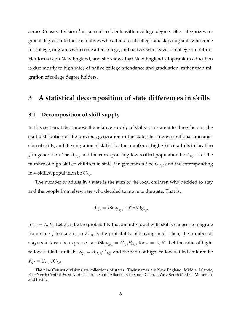
3 A statistical decomposition of state differences in skills

3.1 Decomposition of skill supply

In this section, I decompose the relative supply of skills to a state into three factors: the

skill distribution of the previous generation in the state, the intergenerational transmis-

sion of skills, and the migration of skills. Let the number of high-skilled adults in location

j in generation t be AHjt and the corresponding low-skilled population be ALjt. Let the

number of high-skilled children in state j in generation t be CHjt and the corresponding

low-skilled population be CLjt.

The number of adults in a state is the sum of the local children who decided to stay

and the people from elsewhere who decided to move to the state. That is,

Asjt = #Staysjt + #InMigsjt

for s = L,H . Let Psjkt be the probability that an individual with skill s chooses to migrate

from state j to state k, so Psjjt is the probability of staying in j. Then, the number of

stayers in j can be expressed as #Staysjt = CsjtPsjjt for s = L,H . Let the ratio of high-

to low-skilled adults be Sjt = AHjt/ALjt and the ratio of high- to low-skilled children be

Kjt = CHjt/CLjt.

3The nine Census divisions are collections of states. Their names are New England, Middle Atlantic,East North Central, West North Central, South Atlantic, East South Central, West South Central, Mountain,and Pacific.

6

Using these definitions, the relative skill supply to state j is

Sjt =AHjtALjt

=#StayHjt + #InMigHjt#StayLjt + #InMigLjt

=#StayHjt

(#StayHjt+#InMigHjt

#StayHjt

)#StayLjt

(#StayLjt+#InMigLjt

#StayLjt

)=

CHjtPHjjt

(#StayHjt+#InMigHjt

#StayHjt

)CLjtPLjjt

(#StayLjt+#InMigLjt

#StayLjt

)= KjtΛjtMjt

= Sjt−1Kjt

Sjt−1

ΛjtMjt. (1)

In the above equation, Λjt ≡ PHjjt/PLjjt is the probability of a high-skilled child staying

in j divided by the probability of a low-skilled child staying in the same state. Mjt is a

factor that describes the rate of skill increase through in-migration.

Taking logarithms of Equation 1 yields

ln(Sjt) = ln(Sjt−1) + ln

(Kjt

Sjt−1

)+ ln(ΛjtMjt). (2)

Equation 2 decomposes the relative supply of skills to state j into factors due to the skill

distribution of the previous generation (Sjt−1), the intergenerational transmission of skill

from that generation to the next (Kjt/Sjt−1), and the migration of skills (ΛjtMjt).

I calculate each element of Equation 2 using U.S. Census data. The major benefit from

using Census data is that the samples are large and allow the calculation of skill distri-

butions for many locations. With these data, the location definition is the state, since

that is the most disaggregated level of birthplace identification in the Census. I include

Washington, D.C. as a state.

I use a predicted earnings index to measure skills. I take the full-time workers aged

30 to 40 in the 5 percent 2000 Census sample from IPUMS (Ruggles et al. 2004). With this

7

sample, I estimate a regression of the following form:

yij = βXi +∑k

δkOccik + αj + εij. (3)

The dependent variable, yij , is log weekly labor earnings of individual i who lives in state

j. The vector Xi includes characteristics of individual i: sex, race, a quadratic in age,

and indicators for completed schooling categories. The other regressors are indicators

for three-digit occupation (Occik) and indicators for state of residence. The state of resi-

dence intercepts capture state differences in wages due to various factors, including cost

of living.

Using coefficients from OLS estimation of Equation 3, I predict log weekly labor earn-

ings for all workers, setting the state indicator for New York equal to one and all others to

zero. I define a worker as high-skilled if his or her predicted earnings fall in the highest

quartile of (national) predicted earnings and low-skilled in the lowest quartile. Sjt is the

ratio of high-skilled to low-skilled populations living in state j as adults in 2000. Kjt is

the ratio of high-skilled to low-skilled populations born in state j.

I calculate Sjt−1 using a similar earnings prediction index for an earlier cohort: workers

aged 35 to 45 in the 5 percent 1980 Census sample from IPUMS. I use a regression with

the same form as Equation 3 to predict log weekly earnings for each member of this older

cohort and categorize each member into a quartile of the predicted earnings index. Sjt−1

is the ratio of high-skilled to low-skilled populations living in state j in 1980.

I calculate Psjjt for s = L,H as the fraction of the skill s population born in j who

are also living in j in 2000. I then calculate the relative native retention rate for each

state: Λjt = PHjjt/PLjjt. I also calculate the effect of in-migration on the state skill ratio as

Mjt = Sjt/(Kjt × Λjt).

In order for Equation 3 to predict skills accurately, I assume that the error term εij

does not include interactions between occupation and state of residence. If it did, then

the earnings prediction would confuse productivity of a worker’s state of residence with

8

the worker’s own labor market productivity. I expect productivity differentials between

occupation categories to vary across states less the more narrowly occupations are de-

fined. I use the most narrow occupation coding available.

Previous local skill measures used in the economics literature are average years of

schooling and percent residents with a college degree.4 In the present paper, I adopt a

different measure: the ratio of local high-skilled to low-skilled populations. The main

reason for doing so is that it is the measure most closely related to most economic models

of a geographic distribution of people with heterogeneous skills (eg, Berry and Glaeser

(2005), Glaeser and Saiz (2003), Moretti (2004a)), including the model in this paper. In

addition, this measure uses wages to infer labor market productivity of individual char-

acteristics and captures more variation in skill than schooling alone.5

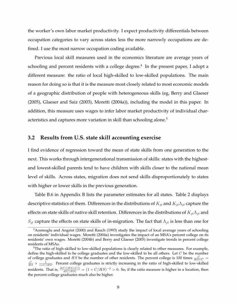
3.2 Results from U.S. state skill accounting exercise

I find evidence of regression toward the mean of state skills from one generation to the

next. This works through intergenerational transmission of skills: states with the highest-

and lowest-skilled parents tend to have children with skills closer to the national mean

level of skills. Across states, migration does not send skills disproportionately to states

with higher or lower skills in the previous generation.

Table B.6 in Appendix B lists the parameter estimates for all states. Table 2 displays

descriptive statistics of them. Differences in the distributions ofKjt andKjtΛjt capture the

effects on state skills of native skill retention. Differences in the distributions ofKjtΛjt and

Sjt capture the effects on state skills of in-migration. The fact that Λjt is less than one for

4Acemoglu and Angrist (2000) and Rauch (1993) study the impact of local average years of schoolingon residents’ individual wages. Moretti (2004a) investigates the impact of an MSA’s percent college on itsresidents’ own wages. Moretti (2004b) and Berry and Glaeser (2005) investigate trends in percent collegeresidents of MSAs.

5The ratio of high-skilled to low-skilled populations is clearly related to other measures. For example,define the high-skilled to be college graduates and the low-skilled to be all others. Let C be the numberof college graduates and HS be the number of other residents. The percent college is 100 times C

HS+C =C

HS ×1

1+C/HS . Percent college graduates is strictly increasing in the ratio of high-skilled to low-skilled

residents. That is, d(C/(HS+C))d(C/HS) = (1 + C/HS)−2 > 0. So, if the ratio measure is higher in a location, then

the percent college graduates much also be higher.

9

all states is a dramatic effect of the relationship between individual skill and migration

behavior. More-skilled people are more mobile, so out-migrants are more skilled than

natives for all states. The fact that Mjt is greater than one for all states shows the same

relationship from the opposite perspective. Table 3 lists correlations between parameters

to show the average relationships between skill measures of states.

The slope coefficient from a regression of ln(Sjt) on ln(Sjt−1) is a measure of generation-

to-generation persistence in local skills. The impact of intergenerational transmission on

generation-to-generation local skill persistence is the relationship between a generation’s

skills and the skills of the next generation if there were no migration. The predicted next

generation skill measure due to intergenerational transmission is ln(Sjt−1) + ln(

Kjt

Sjt−1

).

Similarly, the impact of migration on generation-to-generation local skill persistence is

the relationship between a generation’s skills and the skills of the next generation if there

were no intergenerational transmission. The predicted next generation skill measure due

to migration is ln(Sjt−1) + ln(ΛjtMjt).

Table 4 illustrates the roles that intergenerational transmission and migration play in

determining the persistence of skills across states. Each column represents a separate

regression where observations are states and the variables are skill ratios or predicted

skill ratios. Column 1 includes results from regressing a state’s skill ratio on the skill ratio

of the previous generation in the state. State skill ratios are persistent across generations,

although there is some regression toward the mean in skill. The slope coefficient of the

regression of log skill ratio on previous generation log skill ratio at the state level is 0.65

with a standard error of 0.14. The R2 is 0.32, implying that factors other than the previous

generation’s skills have a large role in determining a state’s skill level.

Figure 1 illustrates this relationship with a scatter plot where I plot for each state the

skill ratio of adults measured in 2000 against the skill ratio of their parents’ generation

measured in 1980. Southeastern states Mississippi, South Carolina, and Arkansas are near

the bottom of both skill distributions. North Carolina started low but gained skills during

this time. Massachusetts gained skills to top the second generation’s skill distribution.

10

Columns 2 and 3 of Table 4 decompose the persistence of local skills into parts due to

intergenerational transmission and migration. The dependent variable in Column 2 is the

state skill ratio if intergenerational transmission were the only mechanism affecting the

geographic skill distribution. This is equivalent to the skill distribution of natives in the

state. I regress this variable on the natural logarithm of the previous generation’s state

skill ratio. The slope coefficient of 0.66 (close to the overall slope of 0.65) implies that

overall mean reversion from generation to generation comes through intergenerational

transmission of skills. Figure 2 plots for each state the second generation’s skills assigned

to their birth states against their parents’ skills. The plot is similar to the one describing

adult locations of these two generations.

This relationship at the location level is comparable to the literature on intergenera-

tional transmission of skills within the family. Solon (1999) surveys the literature on the

intergenerational transmission of earnings. The consensus estimate of the elasticity of

child earnings with respect to parent earnings lies between 0.3 and 0.5 in the U.S. (page

1780). Local skill ratio persistence appears to be higher than family-level intergenera-

tional earnings persistence.

The literature studying the relationship between parents’ schooling and children’s

schooling are also consistent with family-level persistence and some mean reversion. In

cross sections, children’s schooling tends to increase less than one-for-one with parents’

schooling. This is the case in Behrman and Rosenzweig (2002) with U.S. data and in Black,

Devereux, and Salvanes (2005) with Norwegian data. Much of the recent literature on this

topic attempts to decompose the cross-sectional correlation into parts due to genetic and

environmental factors.

The regression in Column 3 of Table 4 has as its dependent variable the state skill ratio

if migration were the only mechanism determining the geographic skill distribution. The

slope coefficient is very close to one, indicating that skill gains through migration are

allocated evenly across states with high and low skills in the previous generation. Figure

3 shows this relationship in a scatter plot. Virginia, Arizona, and Colorado lie above

11

the regression line, so they gain more than average through migration. Iowa, Montana,

Wyoming, and the Dakotas tend to lose skills through migration.

The regression in Column 4 of Table 4 describes the relationship between skills of a

state’s natives and skills of that state’s adults from the same generation after migration.

There is significant persistence in skills from birth to adult locations. Still, adult loca-

tion skills increase less than one-for-one with native skills. In the regression of ln(Sjt) on

ln(Kjt), the slope coefficient estimate is 0.79 with a standard error of 0.1, so the slope is

less than one with 95 percent confidence.

Figure 4 plots for each state the skill ratio of adults in 2000 against the skill ratio of

natives from the same cohort. Massachusetts has the highest ratio of high- to low-skilled

workers at birth and adult residence in this cohort. New York, New Jersey, Connecti-

cut, Washington D.C., and Minnesota are also high-skilled states overall. Southern states

South Carolina, Mississippi, and Arkansas are at the opposite end of the spectrum with

low skill ratios among births and adult residences. Colorado has a medium level of na-

tive skill but gains dramatically through migration. North and South Dakota, Iowa, and

Montana have reasonably high native skills but lose many of them through migration.

4 A model of the geographic distribution of human capital

over time

4.1 Introduction of the framework

The primary purpose of the model is to provide a link from individual skill acquisition

and migration behavior to the geographic distribution of human capital. This will high-

light the mechanisms underlying human capital distributions and provide a framework

for estimating the distributions with individual-level data. A secondary purpose of the

model is to indicate what kinds of labor market characteristics affect local skill levels.

The framework is an over-lapping generations model. There are two decisions that

12

each member of each generation makes. The first is which skill level to acquire as a child.

Skill is indexed by s and takes on values H and L for high- and low-skilled individuals,

respectively. The second decision is where to live as an adult. Individuals can choose to

stay in their origin location or to move to any of the other locations in the economy.

Figure 5 illustrates the timing of events in the model. People are born and grow up in

a labor market. In their birthplace, they decide whether to become high- or low-skilled

workers. They make a migration decision as adults, choosing to stay in their origin or

move to any other labor market. After the migration decision, they work and have chil-

dren in their chosen location and die. Members of the new generation then make the

skill investment and migration decisions and have children and work in their chosen lo-

cation. Each labor market clears in each period (generation) so that the relative supply of

high- to low-skilled workers in each labor market equals the relative demand for high- to

low-skilled workers there.

4.2 Decomposition of local relative supply of skills

The local supply of skills is the aggregation of skill acquisition and migration decisions. I

describe skill acquisition and then migration decisions. I then aggregate them to represent

local relative skill supply.

LetUsij be the net benefit to individual i growing up in location j of having skill level s.

This is a function of expected benefits and costs to investing in skills. Individual i chooses

to invest in high skills if UHij − ULij > 0 and chooses low skills otherwise. Let ParHi be

an indicator for child i having high-skilled parents and zj be a vector of characteristics of

i’s origin location j. The following equation represents net benefits of high relative to low

skill acquisition for individual i:

UHij − ULij = α1 + α2ParHi + α3zj + α4ParHizj − εij.

Parents’ skills affect the costs of acquiring skill, as do location characteristics in zj , such

13

as proximity to college. Assume εij ∼ N(0, 1). Then, the following formulas measure skill

acquisition rates:

PHLj = Φ(α1 + α3zj)

PHHj = Φ(α1 + α2 + (α3 + α4)zj).

Φ(·) is the standard normal cumulative distribution function. PHLj is an estimate of the

probability a child growing up with low-skilled parents in a location with characteris-

tics zj will be high-skilled. PHHj is the probability a child growing up with high-skilled

parents in a location with characteristics zj will be high-skilled.

The next decision individuals make is where to live when adults.6 Let s(i) be a func-

tion that gives the skill level of individual i and b(i) be a function that gives the birthplace

of individual i. The utility that individual i attains from residing in location k in genera-

tion t is

Vikt = γ ln W̄s(i)kt + βs(i)tzb(i)kt + εikt,

where W̄s(i)kt is the location k average wage among residents with skill level s and zb(i)kt

is a vector of location characteristics. This vector includes interactions between origin

and destination characteristics, so individuals from different origins attach different val-

ues to destination characteristics. For example, distance between origin and a potential

destination is allowed to enter Vikt.

Note also the treatment of wages. Average wages enter the utility function, which

could be justified by assuming individuals have imperfect information about wages they

will be able to earn in any given location. This is unrealistic but perhaps not extreme in

this context, where my focus is on estimating average preferences and behavior. More-

over, I constrain the marginal utility of labor earnings (γ) to be the same for both skill

6The model at present does not allow the skill acquisition and migration decisions to interact. Theprimary reason is simplicity, both in model exposition and estimation. If children acquire skills becausethey are anticipating their use of those skills in some labor market other than their origin, then this methodwill mistakenly identify location characteristics as inducing migration instead of the acquisition of skills.

14

levels.

The residual εikt is distributed extreme value independently and identically across i, k,

and t. This distribution of the residuals implies that the probability of utility-maximizing

individual i locating in k is (letting i’s origin be j and i’s generation be t)

Pijkt =exp(γ ln W̄s(i)kt + βs(i)tzjkt)∑l exp(γ ln W̄s(i)lt + βs(i)tzjlt)

. (4)

See McFadden (1974).

I now aggregate the skill acquisition and migration decisions in order to characterize

the relative supply of skills to a labor market. I take notation from the accounting exercise

above, so Sjt = AHjt/ALjt is the relative supply of high- to low-skilled adults of generation

t to location j, and Psjkt is the probability that an individual with skill s chooses to migrate

from location j to location k. I add here that an expression for the number of in-migrants

to j with skill level s is #InMigsjt =∑

k 6=j CsktPskjt. Then, following Equation 1, the

location j relative supply of skills can be expressed as

Sjt =CHjtPHjjt

(Pk CHktPHkjt

CHjtPHjjt

)CLjtPLjjt

(Pk CLktPLkjt

CLjtPLjjt

) . (5)

I can decompose this supply into the intergenerational transfer mechanism and migra-

tion. The former is the mechanism that maps local parents’ skills into local children’s

skills. Define the skill transmission function to be

Kj

(AHjt−1

ALjt−1

)=

(AHjt−1/ALjt−1)PHHj + PHLj(1− PHLj) + (AHjt−1/ALjt−1)(1− PHHj)

=AHjt−1PHHj + ALjt−1PHLj

ALjt−1(1− PHLj) + AHjt−1(1− PHHj)=CHjtCLjt

. (6)

Defining Kj as a function rather than a multiplier, as in the accounting exercise, allows

a more explicit treatment of intergenerational transmission, which is possible with the

NELS:88. Further define Λjt = PHjjt/PLjjt to describe the effect of retention of natives on

15

the local skill distribution. Finally, define

Mjt =

(∑k CHktPHkjtCHjtPHjjt

)/(∑k CLktPLkjtCLjtPLjjt

)

to describe the effect of in-migration on the local skill distribution. Mjt is the growth of

high skills relative to the growth of low skills through in-migration.

Plugging these definitions into Equation 5, the evolution of relative skills in location j

follows

Sjt = Kj(Sjt−1)× Λjt ×Mjt. (7)

I will estimate each element of this equation in order to assess how the intergenerational

transmission of skills and migration contribute to the geographic distribution of skill.

4.3 Equilibrium in local labor markets

Each labor market of the model clears in every period (generation). Equilibrium is reached

when the relative supply of skills in each labor market equals the relative demand for

skills. The relative supply of skills to labor market j is, plugging the location choice prob-

abilities of Equation 4 into the supply Equation 1,

Sjt =AHjtALjt

=#StayHjt + #InMigHjt#StayLjt + #InMigLjt

=

∑k CHktPHkjt∑k CLktPLkjt

=

∑k CHkt

(exp(γ ln W̄Hjt+βHtzkjt)Pl exp(γ ln W̄Hlt+βHtzklt)

)∑

k CLkt

(exp(γ ln W̄Ljt+βLtzkjt)Pl exp(γ ln W̄Llt+βLtzklt)

)=

exp(γ ln W̄Hjt)∑

k CHkt

(exp(βHtzkjt)P

l exp(γ ln W̄Hlt+βHtzklt)

)exp(γ ln W̄Ljt)

∑k CLkt

(exp(βLtzkjt)P

l exp(γ ln W̄Llt+βLtzklt)

)

16

Let sjt ≡ ln(Sjt) and wjt ≡ ln(W̄Hjt/W̄Ljt). Then, the relative supply of skills to location j

is

sjt = γwjt + Ψjt, (8)

where Ψjt is a function of attributes of location j at time t relative to other locations.

Let Djt be the local relative demand for high- and low-skilled individuals, and djt ≡

ln(Djt). The following equation describes the local relative demand for skills:

djt = −σwjt + ejt. (9)

γ and σ are positive parameters that represent elasticities with respect to the local relative

wage.7

In equilibrium, each local labor market must clear so that sjt = djt. This implies the

following:

djt = sjt =γ

γ + σejt +

σ

γ + σΨjt. (10)

The local skill premium is

wjt =ejt −Ψjt

γ + σ.

Relative wages tend to be higher in labor markets with strong relative demand for skills

(ejt) and lower in labor markets with amenities valued more by higher- than lower-skilled

workers (Ψjt).

The rate of growth in local relative skills that comes through migration is given by the

7This representation of local relative labor supply and demand draws upon Bound, Groen, Kezdi, andTurner (2004).

17

term Λjt ×Mjt in Equation 7. 8 In equilibrium, the following holds:

ln(Λjt ×Mjt) = sjt − ln[Kj(Sjt−1)]

=γ

γ + σejt +

σ

γ + σΨjt − ln[Kj(Sjt−1)]. (11)

This equation makes clear that relative skill flows from migration depend upon current

location characteristics (relative to other locations) that affect relative demand and supply,

previous generations’ location decisions, and the local intergenerational transmission of

human capital. This is a reduced form equation I will estimate in order to identify char-

acteristics of labor markets that draw skills through migration.

An important feature of the model to keep in mind is that quantities are always ratios.

As a result, local characteristics that affect high- and low-skilled individuals in the same

way do not affect the equilibrium relative skill level. For example, cost of living that

deflates all nominal wages in a city by the same proportion should not have an effect on

the local relative supply of skills. Amenities that are valued the same between high- and

low-skilled individuals should not affect the relative supply of skills. Amenities that are

normal goods, however, will tend to draw the higher skilled (with higher incomes) at

higher rates.9

8To see this, note that

Λjt ×Mjt =PHjjt

(Pk CHktPHkjt

CHjtPHjjt

)PLjjt

(Pk CLktPLkjt

CLjtPLjjt

)=

Pk CHktPHkjt

CHjtPk CLktPLkjt

CLjt

=∑

k CHktPHkjt/∑

k CLktPLkjt

CHjt/CLjt

9Cost of living and amenities in this model do affect total population flows into and out of locations, butmy focus will be on relative flows of high- and low-skilled populations.

18

5 Data description

The location definition in this study approximates a labor market, which I consider to

be the smallest geographic space where most residents work and most workers reside. I

use the commuting zone (CZ) as the location definition. Tolbert and Sizer (1996) describe

the identification of CZs using journey-to-work data from the 1990 Census. Each CZ is a

collection of counties (or single county) that share particularly strong commuting links.

The CZ definition has the added feature of encompassing both rural and urban areas.10

There are 741 CZs in the U.S. 604 of them are entirely contained by a single state, 129 of

them by two states, and 8 of them by three states (eg, Washington, D.C.). CZ populations

in 2000 range from 1,193 (Murdo, SD) to 16,393,360 (Los Angeles, CA). 258 CZs contain a

metropolitan statistical area.

I calculate some average characteristics of CZs with the U.S. Census. I use the 1990 and

2000 5 percent samples available through IPUMS. These characteristics include average

wages, percent with college degrees, and percent employment in manufacturing. The

smallest identifiable area in the Census is the public use microdata area (PUMA), which

is a Census-defined place with population no less than 100,000. This definition does not

allow perfect matching of boundaries for all CZs. The method used to convert PUMA

averages to CZ averages involves assigning PUMA characteristics to a CZ based on the

population weight of the PUMA in the CZ. The data appendix includes a more detailed

description of the method.

Additional CZ characteristics come from various sources. I aggregate CZ population

from county population files available through IPUMS. Region and urban status come

directly from Tolbert and Sizer (1996). I calculate average climate characteristics (such as

average temperatures and snowfall) using data from the National Climatic Data Center. I

characterize CZs as being coastal if at least one of the counties making up the CZ has an

ocean coastal property. The distance between two CZs is the great circle distance between

10This is the same location definition used in Autor and Dorn (2007) to study the interactions of differenttypes of workers within labor markets.

19

their latitude and longitude coordinates, in kilometers.

I use state higher education appropriations and public college tuition data from Fortin

(2007). From the data Fortin make available, I calculate higher education appropriations

per full-time equivalent student and public tuition per public college student for each

state. The higher education subsidy variable I use in some specifications is the appropri-

ations variable divided by the tuition variable.

I also calculate college enrollment for each CZ. I acquire college enrollment in each

county from the Integrated Postsecondary Education Data System (IPEDS) at the National

Center for Education Statistics (NCES) and sum over counties to get CZ enrollments. The

enrollment measure is the full-time equivalent number of undergraduate students at two-

year and four-year colleges.

I use state wage and capital tax data from Daniel Feenberg at the National Bureau of

Economic Research (NBER). The variables I use are the highest marginal tax rates that

people face in each state. These rates combine Federal and state taxes. Information about

the program used to calculate tax rates (TAXSIM) is available in Feenberg and Coutts

(1993).

CZs sometimes consist of counties in more than one state. For state-level variables

(higher education appropriations, tuition, and tax rates), I assign to each CZ the charac-

teristics of the state with the larger share of CZ population.

Table 5 displays descriptive statistics for the 741 CZs. The range of percent residents

with college degrees from Table 1 is repeated. People choosing residential location have a

set of choices that is very diverse along many dimensions, which helps identify character-

istics that contribute to the skill distribution. The range of average wages, temperatures,

industry structures, populations, tax policies, and subsidy rates for public higher educa-

tion are all quite large.

To investigate both the intergenerational transmission of skill and early migration de-

cisions, I use the National Education Longitudinal Study of 1988 (NELS:88). Several fea-

tures of the NELS:88 address the weaknesses of using the Census for the present pur-

20

poses. First, the restricted-use version of the NELS:88 has zip code data that identify the

CZ of residence for each respondent, both in 8th grade and at age 26. Second, the NELS:88

includes more informative data on individual skills and family background, most notably

test scores and parent’s education. Third, the NELS:88 has information about the parents

of each respondent, allowing investigation of the intergenerational transmission of skill

at the family level. Fourth, the NELS:88 identifies location of respondents at 8th grade,

which is more likely to approximate the location of skill acquisition than the birth state in

the Census data.

NELS:88 data collection began with a representative sample of students in the eighth

grade of U.S. schools in 1988. Follow-up surveys were completed in 1990, 1992, 1994,

and 2000. In the final follow-up, students were around 26 years old and mostly out of

school. They were making early family formation and labor market decisions, including

geographic location choices. Labor market information includes annual earnings and

whether full-time, in addition to occupation and industry.

Figure 6 implies that a weakness of the NELS:88 data for my purposes is the relatively

young age at final follow-up. Figure 6 plots different types of average migration rates

from the 2000 Census by age. The series refer to migration defined as changing houses,

changing PUMAs, and changing states between 1995 and 2000. Five-year migration rates

peak around the age of the final location information from NELS:88 respondents. The

model above includes a single location decision for each agent, which may not be ap-

proximated well by the relatively early location decisions in these data.

Table 6 provides summary statistics for the NELS:88 sample I use. There are 11,079

respondents with non-missing location information in 8th grade and the 2000 follow-up

survey. For this table and all estimation with the NELS:88, I apply sample weights that

make the NELS:88 sample representative of 8th grade students in U.S. schools in 1988.

Table 6 also shows that migration out of one’s origin CZ is common. About 35 percent of

respondents lived at age 26 in a CZ other than their 8th grade CZ.

Migration behavior varies substantially across skill levels and family backgrounds.

21

Table 6 shows that college graduation, the test score index, parent’s education, parent’s

income, and early labor market earnings are all higher for those who had migrated away

from their 8th grade labor market. The test score index is defined such that a 0.1 increase

in the index represents a change in math and verbal scores on an 8th grade test that predict

a 0.1 increase in log earnings.11

6 Estimation of the model and results

6.1 Estimation of model parameters

In estimation, I depart from the model in one significant way. When defining skill cate-

gories of parents and children, I allow there to be four skill levels instead of two. I use

four skill levels in order to have more of a distinction between high- and low-skilled indi-

viduals than splitting the sample in half would yield, while using all of the data available.

The first step in estimating the model is measuring, for each U.S. labor market, the

skill distribution of the generation of NELS:88 parents. I take this cohort to be workers

in the 5 percent 1990 Census who were ages 34 through 56. With full-time workers from

this sample, I estimate Equation 3 by OLS. I use coefficients from this regression to pre-

dict log weekly labor earnings for all workers, setting the state indicator for New York

equal to one and all others to zero. High-skilled people make up the highest quartile of

the national predicted earnings distribution, and low-skilled people make up the lowest

quartile. The estimate of Sjt−1, the skill ratio in labor market j among the parent genera-

tion, is the ratio of high-skilled to low-skilled populations in CZ j.

The next steps in estimating the model are estimating the intergenerational transmis-

sion of skill and location choice models with the NELS:88. I categorize NELS:88 respon-

dents into skill categories that correspond with quartiles of a predicted earnings distri-

bution. The form of the regressions is similar to the one used with the Census, although

11The index ranges from 9.950 to 10.145. The index at mean eighth grade test scores is 10.030. The index atone standard deviation higher on verbal and math scores is 10.052, representing a gain in predicted annualearnings of about 2 percent.

22

earnings predictions with the NELS:88 use data on test scores and parents’ education but

not occupation. The other difference is that I measure annual earnings in the NELS:88

rather than weekly earnings.

I also categorize NELS:88 parents into skill groups. Characteristics of parents are

somewhat limited, and the earnings data seem less reliable than for their children (re-

spondents). So, I define parent skills by a ranking of completed schooling and family

income. I rank the parents by years of schooling of the parent with the higher value. This

is a categorical variable and does not induce equal quartiles. So, within years of school-

ing, I rank parents by their family income. I then define the parents in the highest quartile

of this education and income ranking to be high-skilled and parents in the lowest quartile

to be low-skilled.

I then estimate separate probit models for students attaining each skill level, as func-

tions of parents’ skill categories and characteristics of the origin CZ. The results from

these probit models are in Table B.1 of Appendix B. As expected, the skill level of par-

ents is a clear predictor of child skill. Some location characteristics are correlated with

the skill acquisition of local youth. These specifications include many location character-

istics, making interpretation of marginal effects difficult. For example, the coefficient on

log college subsidy needs to be interpreted as the partial effect of subsidies controlling for

variables including college enrollment per capita, wage taxes, local wages, and percent

residents with college degrees. The purpose of including so many variables is to capture

much of the variation across labor markets in the intergenerational transmission of skills.

One of these probit models estimates the probability a high-skilled parent in a CZ

with the characteristics of j will have a high-skilled child. In model language, this is an

estimate of PHHj . The probit models also estimate the probabilities of intergenerational

skill transfer between all pairs of parent and child skill types in all CZs. Using these, I

calculate the model parameterKj(Sjt−1) for each labor market j, using the estimated Sjt−1

from the Census and a four-skill analogue of Equation 6.12

12More specifically, let MH and ML denote medium-high and medium-low skills, respectively. Theserefer to the second-highest and third-highest quartiles in the predicted earnings index. From the 1990

23

Next, I estimate migration probabilities using a separate logit model for each skill cat-

egory, where the choice is among CZs of residence. The form of the logits that I estimate

uses the following specification for the utility to individual i living in CZ k:

Vik = γs(i) ln W̄s(i)k + βs(i)1Homeik + βs(i)2Distanceik + βs(i)3Distance2ik

+ βs(i)4zk + βs(i)5Homeikzk + βs(i)6Ruralb(i)zk + βs(i)7zkzb(i) + εik,

where Homeik is an indicator for k being i’s origin CZ, Distanceik is the distance in kilo-

meters between k and i’s origin CZ, Ruralb(i) is an indicator for i’s origin CZ being rural,

zk is a vector of destination characteristics, and zb(i) is a vector of origin characteristics. I

estimate W̄s(i)k for each destination as the average wage of local workers in skill category

s. I do not constrain γs(i) to be the same across skill levels as the model assumes.

Tables B.2 through B.5 display parameters from four logit models that estimate loca-

tion choices of NELS:88 respondents. The coefficient on local average wages is negative

for three of the skill groups. In reality, destination choices depend on both supply and

demand factors, so the coefficient on average wages can be positive or negative. One

would not expect this estimate necessarily to be consistent for the slope of the relative

supply curve. In addition, the average wage measure I use is surely different from the

offer wages that workers receive. Other local characteristics appear to affect utility more

than this average wage measure.

The coefficients on Homeik show that people of all skill levels are much more likely

to stay in their labor market of origin than move to another. There is also a significant

utility reduction associated with distance from origin, and this is quite consistent across

skill levels.

Census, I estimate local adult populations AHjt−1, AMHjt−1, AMLjt−1, and ALjt−1. Then, estimates of thenext generation’s child skill populations are

CHjt = AHjt−1PHHj + AMHjt−1PHMHj + AMLjt−1PHMLj + ALjt−1PHLj

CLjt = AHjt−1PLHj + AMHjt−1PLMHj + AMLjt−1PLMLj + ALjt−1PLLj

and Kj(Sjt−1) = CHjt/CLjt.

24

Conditional on other location characteristics, the Northeast is the least attractive des-

tination for all skill levels, and the West is the most attractive destination for all except

low-skilled individuals. The percent college at origin tends to encourage people to leave,

although the percent college of non-home destinations tends to be a positive amenity (or

it is correlated with some other positive amenity in the residual). This is most clearly the

case with higher-skilled individuals.

In model language, the logit models yield estimates of PHjkt and PLjkt for all combina-

tions of labor markets j and k, including j = k. With these, I calculate Λjt = PHjjt/PLjjt

and Mjt =(P

k CHktPHkjt

CHjtPHjjt

)/(Pk CLktPLkjt

CLjtPLjjt

)for each j, where CHjt and CLjt come from the

procedure used to calculate Kj(Sjt−1) (see Footnote 12). The final parameter to estimate

is Sjt = Kj(Sjt−1)ΛjtMjt for each j.

As a robustness check, I estimate the model with the NELS:88 using states instead

of CZs as locations. If the model estimation procedure is reliable, then this exercise will

replicate findings from the accounting exercise that uses Census data alone. For the most

part, this is the case. I describe the results in Appendix C. Overall, model estimation with

the NELS:88 has enough precision to replicate findings in the Census, and this adds cred-

ibility to the procedure for understanding the geographic distribution of human capital.

6.2 Model estimation results about the geographic distribution of hu-

man capital

Figures 7 through 10 illustrate the persistence of skills in CZs from generation to gener-

ation. Tables 7 through 13 describe how migration and intergenerational transmission

interact with skills of labor markets. The results indicate that intergenerational trans-

mission causes some regression to the mean of skills across CZs, as it does across states.

Migration works against this tendency across CZs, unlike across states. That is, migration

transfers more skills to CZs that had higher parent skills. Intergenerational transmission

transfers skills toward smaller and more rural labor markets, while migration transfers

25

skills toward larger and more urban labor markets. Overall, CZs that gain more skills

tend to be larger and to have lower temperatures in January, higher supplies of higher

education services, and more taxation of wages relative to than capital.

Table 7 displays descriptive statistics of model estimates for CZs with the NELS:88.

The variation in skills across CZs is dramatic. Take, for example, the parent generation

skill ratios estimated with the 1990 Census. They range from 0.28 to 1.87. Also, the skew-

ness of the distribution of skills across CZs at adult residence (3.8) is higher than the

skewness of the child skill distribution (1.12). Migration contributes to skewness in the

skill ratio distribution, as a few CZs accumulate high rates of skill.

The mean of adult skill ratios across labor markets (Sjt = 0.92) is smaller than the mean

of skill ratios for children (Kj(Sjt−1) = 1.11). The national sample has an equal number

of high- and low-skilled individuals, by definition. The mean of skill ratios across labor

markets need not equal one, however, because CZs get equal weight in these averages,

although their populations differ dramatically. When larger CZs tend to have higher skill

ratios, the average of skill ratios is below one. So, migration tends to move skills toward

larger CZs. Also, the mean of parent skill ratios (Sjt−1 = 0.77) is smaller than the mean

of child skill ratios (Kj(Sjt−1) = 1.11). This implies that intergenerational transmission

tends to move skills toward smaller CZs.

Table 8 lists correlations between parameters from the model. The correlation between

intergenerational transmission’s effect on the skill ratio (Kj(Sjt−1)/Sjt−1) and pre-existing

skill (Sjt−1) is -0.448. This reflects mean reversion in skills through intergenerational trans-

mission. The correlation between the total migration effect on the skill ratio (ΛjtMjt) and

the parent generation skills (Sjt−1), on the other hand, is positive (0.241). So, migration

across CZs tends to work against the mean reversion due to intergenerational transmis-

sion.

In addition, skills of the previous generation’s adults predict skills of the next gen-

eration’s adults: the correlation between skill ratios Sjt−1 and Sjt is 0.453. The intergen-

erational transmission effect on skills is negatively correlated with the total migration

26

effect on skills. That is, the correlation between Kj(Sjt−1)/Sjt−1 and ΛjtMjt is -0.273. This

is consistent with intergenerational transmission moving skills to smaller labor markets

and migration moving skills to larger labor markets. Native retention of skills (Λjt) is

negatively correlated with in-migration of skills (Mjt); this correlation is -0.35.

It is likely that model estimation with the NELS:88 adds extra sampling variation that

is not present in estimates relying only on Census data. Comparisons between the stan-

dard deviation and skewness of Sjt−1 and other parameters such asKj(Sjt−1) and Sjt may

be misleading, since Sjt−1 is estimated with 1990 Census data only. In particular, the stan-

dard deviation of Sjt−1 being lower than the standard deviations ofKj(Sjt−1) and Sjt may

be the result of sampling variation rather than an increase in the inequality of skills across

CZs over time. In addition, extra variation of a variable that is bounded below by zero,

like these ratios, likely induces right skewness. So, I do not make much out of the increase

in skewness from Sjt−1 to Kj(Sjt−1). However, comparisons between Kj(Sjt−1) and Sjt,

which both use the NELS:88 to estimate distributions of CZs, seem more reliable.

I turn next to quantifying the effects of intergenerational transmission and migration

on the generation-to-generation persistence of CZ skills.13 Column 1 of Table 9 displays

results from a regression of the log skill ratio for adults in a CZ on the log skill ratio in

that CZ of the previous generation. The slope coefficient is clearly less than one, so there

appears to be some mean reversion. The R2 of 0.22 indicates that factors other than the

previous generation’s skills play a significant role in determining the current generation’s

local skills. Figure 7 illustrates this relationship with a scatter plot.

Column 2 of Table 9 has results from a regression where the dependent variable is

a prediction of what the CZ’s adult log skill ratio would be if there were no migration.

This is the same as the log skill ratio among children in the CZ. The independent variable

in the regression is the previous generation’s log skill ratio. The coefficient estimate is

lower than the coefficient from Column 1, indicating that intergenerational transmission

13At present, the results on persistence assume the model parameters are estimated without error. To theextent that they have sampling error, the persistence results are biased, with the effects of the bias increasingwith the variability of the estimates. I am working on estimating the extent of sampling error to correct forthis potential bias.

27

is driving the overall mean reversion. Figure 8 illustrates this relationship with a scatter

plot.

Migration works against mean reversion by moving more skills to CZs with higher

parents’ skills. The regression in Column 3 of Table 9 has as its dependent variable the

predicted CZ log skill ratio if there were no intergenerational transmission effect on skills.

This equals the sum of the log parent skill ratio and the log migration effect: ln(Sjt−1) +

ln(ΛjtMjt). The coefficient estimate is greater than one, indicating that CZs with higher

parent skill ratios gain more skills through migration than others. Figure 9 illustrates this

relationship. The points are distributed more tightly around the regression line than the

plots involving intergenerational transmission. Selective migration is relatively tightly

linked with the previous generation’s skills.

The regression in Column 4 of Table 9 describes the relationship between skills of

children in a CZ and the skills of adults from the same cohort in the CZ after migration

choices are made. The coefficient estimate is 0.858 with a standard error of 0.034. There

is substantial persistence between child and adult local skills, but the slope is less than

one. So, adult skills increase less than one-for-one in child skills. Figure 10 illustrates this

relationship.

Comparison between Columns 3 and 4 of Table 9 reveals that the previous genera-

tion’s adult skills in the CZ has a stronger effect on skilled migration to the CZ than the

skills of the same generation as children. The slope coefficient and R2 are both higher in

the regression on parent skills. This implies that different location characteristics predict

the skills of local children and adults. In particular, it is consistent with previous findings

that high-skilled adults tend to move to larger CZs, while intergenerational transmission

tends to move high-skilled children toward smaller CZs.

Tables 10 through 15 display results from regressions of model parameters on location

characteristics. Overall, the results show that small labor markets lose skilled workers at

high rates through migration. Other local characteristics, such as higher education policy,

weather, and taxes, also affect the local skill mix. The intergenerational transmission of

28

skills contributes to mean reversion of local skills, as small CZs gain more than larger

CZs through migration. Skilled migration, on the other hand, contributes to persistence

of inter-location inequality in skills, as large and urban CZs with the highest skill levels

among the previous generation gain the most skills through migration.

Table 10 displays a series of regressions that describe characteristics of CZs that affect

the degree to which migration behavior shifts the local skill distribution (ln(Λjt ×Mjt)).

This specification follows Equation 11 from the model. Column 1 reiterates the negative

correlation between native skill and the skill content of migration. This is not a par-

ticularly large offsetting force to a change in local native skills, however. For example,

if Kj(Sjt−1) increases by 10 percent, then on average the off-setting decrease in ΛjtMjt

means that Sjt = Kj(Sjt−1)ΛjtMjt still increases by about 8.5 percent.

Western labor markets gain the most skill through migration. Small and rural labor

markets acquire significantly less skill through migration than large cities. The specifi-

cation in Column 2 implies that an average major metropolitan area in the West gains 5

high-skilled migrants for every 4 low-skilled migrants, whereas an average small town in

the West gains only 3 high-skilled migrants for every 4 low-skilled migrants.14 The differ-

ences in skilled migration across population categories remain large after controlling for

a battery of other CZ characteristics.

CZs with colder winters (measured with average January temperature) gain more skill

through migration than warmer labor markets. College enrollment per capita and state

college subsidies are both positively correlated with skill gains through migration. The

college subsidy variable is state higher education appropriations per public college stu-

dent divided by average public college tuition. The tax structures of places gaining skills

through migration tend to be tilted toward wage taxes and away from capital taxes. Col-

umn 7 demonstrates that the previous findings hold when not controlling for initial skill

mix of native children.14This statement uses figures for non-coastal CZs in the West. Due to the log specification, which esti-

mates a proportional effect, these level differences are smaller for other regions, where the average level ofskilled migration is smaller.

29

Table 11 shows local characteristics that are correlated with the local intergenerational

transmission of skill, here defined as ln(Kj(Sjt−1)) − ln(Sjt−1). The first row repeats the

negative correlation between parents’ skill ratio and gains from intergenerational trans-

mission. This negative correlation remains after controlling for a battery of local charac-

teristics. Smaller CZs gain more skill through intergenerational transmission than larger

CZs, and small towns gain the most. This confirms results above that imply intergener-

ational transmission tends to move skills toward smaller CZs, in contrast to migration,

which moves skills toward larger CZs (see Table 10).

Local college enrollment and state college subsidies are positively correlated with skill

gains through intergenerational transmission. The college subsidy effect becomes larger

after controlling for state taxes. College subsidies conditional on state tax levels proxy for

the emphasis placed on higher education in the state budget. Conditional on state taxes

and other controls, an increase in this subsidy of 10 percent is correlated with an increase

in the rate of skill gain through intergenerational transmission of about 1 percent. CZs

with colder Januaries tend to gain more skill through intergenerational transmission, as

do CZs in states with lower capital taxes. Manufacturing is positively correlated with the

intergenerational transmission of skill.

The next two tables identify correlates with the effects on local skills of natives leaving

and of others migrating into the area. The dependent variable in Table 12 is the rela-

tive native retention rate ln(Λjt). Locations with higher skills among their children tend

to keep a higher rate as some natives decide to leave. Major metropolitan areas retain

skills at the highest rates, and larger rural labor markets lose the most skills through out-

migration. College supply factors are negatively correlated with the retention of skills. It

is possible that local college supply is a reaction to the loss of skilled natives or that local

colleges are correlated with factors that increase the mobility of skilled native children.

Table 13 shows that a higher skill mix of native stayers is correlated with a lower skill

mix of in-migrants. Small rural CZs experience much less skilled in-migration than major

metropolitan areas. Specifications that do not control for the skill ratio of native stayers

30

imply a relatively high rate of skill gain through migration for larger rural CZs. This is

the category of CZs that experiences the greatest loss of skills through out-migration, so

controlling for stayers’ skills makes a large difference.

Skilled migrants appear to be drawn to colder CZs. More-skilled migrants appear to

value college supply factors more than less-skilled migrants. The taxes of places gaining

skill through migration are tilted toward wage taxes and away from capital taxes. CZs

with a higher manufacturing share of industry tend to gain less skill through migration.

The next two tables display correlates with skill ratios, rather than mechanisms that

change skill ratios. The dependent variable of specifications in Table 14 is the natural log-

arithm of the skill ratio of native children, ln(Kj(Sjt−1)). The first row shows that parents

transferring skills to their children contribute to the persistence of inequality across loca-

tions, although there is substantial regression to the mean, repeating the specification in

Column 1 of Table 9. This persistence in skills remains after controlling for labor market

size, region, weather, college supply, tax rates, and local manufacturing. These parame-

ters indicate that initial skill inequality across CZs would become quite small after a few

generations, absent any migration.

Warmer Januaries are negatively correlated with native skills. An increase in average

January temperature of 10 degrees (F.) is correlated with a decrease of the native chil-

dren skill ratio of about 12 percent. The native children skill ratio is increasing in college

enrollment and the subsidy rate for college.

Conditional on the local parent generation’s skill ratio, smaller CZs tend to have

higher levels of native skill. The specification in column 8 that does not condition on

parent generation skills reveals a much less clear relationship between CZ size and na-

tive skill ratio, where small towns and major metropolitan areas have the most-skilled

children. The highest proportions of skilled children are in the Northeast and Midwest.

Table 15 displays results from regressing the natural logarithm of adult (post-migration)

skill ratios (ln(Sjt)) on local characteristics. The first row shows the persistence of local

skills across generations, which is significant but not complete, repeating the Column 1

31

specification of Table 9. Column 2 of Table 15 shows a specification that does not control

for the previous generation’s skill ratio. Skill ratios increase in CZ size. Controlling for

the previous generation’s skill ratio flattens this gradient somewhat, but doing so shows

that even small towns at similar starting points end up after a generation with signifi-

cantly lower skills than larger CZs. Subsequent specifications show that colder CZs and

those with more higher education supply tend to have higher skill ratios. Taxes tend to

tilt toward wage taxes and away from capital taxes in CZs with high skills. Higher man-

ufacturing shares predict higher skills but only when conditioning on previous skills.

7 Conclusion

This paper examines the determinants of labor market skill distributions. The framework

decomposes labor market supplies of skills into the previous generation’s skills, the in-

tergenerational transfer of skill from local parents to their children, and the migration of

people with different skill levels. I estimate parameters that describe these factors with

a combination of Census and NELS:88 data sets. The model estimates replicate the main

findings from an accounting exercise for state skills that uses the Census and fewer model

assumptions.

I find that intergenerational transmission of skills contributes to mean reversion of

local skills. This is true across states and labor markets defined as commuting zones

(CZs). More specifically, smaller CZs tend to gain the most skill through intergenerational

transmission. Migration across CZs works against this mechanism. CZs with higher skills

in the previous generation gain more skill through migration. This manifests in high rates

of skilled migration toward larger and more urban CZs at the expense of smaller and more

rural CZs. In this way, migration adds to persistence over time in skill inequality across

CZs.

I also estimate correlations between other labor market characteristics and skilled mi-

gration. Skilled migrants are drawn to the West and to colder climates. Skill growth is

32

higher in states with tax structures tilted toward wage taxes and away from capital taxes.

I find that the relationship between local college supply factors and skilled migration

is positive and substantial. The estimates here assume that college supply factors are

exogenous. It is likely, however, that other factors influencing skilled migration are cor-

related with local college supply. An example is a local industry that both supports local

university research and also hires many college graduates from outside the area. It would

be useful from a policy perspective to estimate the effect of local college supply on skilled

migration. The challenge would be to find some variation in local college supply that is

orthogonal to other causes of skilled migration. Since colleges typically open and close

infrequently and expand slowly, it is difficult to find such variation at the institutional

level. Tuition policies may display more useful variation.

The results presented here, in particular about the persistence of skill inequality, are

potentially sensitive to bias due to sampling error of model estimates. This is an errors-

in-variables issue similar to that raised in Deaton (1985) and studied recently in Devereux

(2007). So far, I assume that model parameters are estimated without error. This is clearly

not true. I am working on estimating the sampling error in the model estimates in order

to correct for potential bias in regressions of model parameter estimates on other model

parameter estimates. Regressions of model parameters exclusively on CZ characteristics,

such as Column 2 of Table 10, should not be susceptible to this bias.

A weakness of this analysis is that the NELS:88 only follows individuals to age 26. As

Figure 6 makes clear, many migration decisions occur after this age, so it is not clear that

NELS:88 respondents have settled down in the labor market where I last observe them to

reside. I plan to estimate the parameters of the model using data from the National Lon-

gitudinal Survey of Youth, 1979 (NLSY79). This panel data set has many of the attractive

features of the NELS:88, and the NLSY79 respondents are interviewed much later in their

life cycles.

33

References

[1] Acemoglu, Daron and Joshua Angrist (2000) “How Large are the Social Returns to

Education? Evidence from Compulsory Schooling Laws” NBER Macroannual 9-59.

[2] Autor, David and David Dorn (2007) “Inequality and Specialization: The Growth of

Low-Skill Service Jobs in the United States” working paper.

[3] Basker, Emek (2003) “Education, Job Search and Migration” working paper.

[4] Behrman, Jere R. and Mark R. Rosenzweig (2002) “Does Increasing Women’s School-

ing Raise the Schooling of the Next Generation?” American Economic Review 92(1)

323-334.

[5] Berry, Christopher R. and Edward L. Glaeser (2005) “The Divergence of Human Cap-

ital Levels across Cities” Papers in Regional Science 84(3) 407-444.

[6] Black, Sandra E., Paul J. Devereux, and Kjell G. Salvanes (2005) “Why the Apple

Doesnt Fall Far: Understanding Intergenerational Transmission of Human Capital”

American Economic Review 95(1) 437-449.

[7] Borjas, George J., Stephen G. Bronars, and Stephen J. Trejo (1992) “Self-Selection and

Internal Migration in the United States” Journal of Urban Economics 32, 159-185.

[8] Bound, John, J. Groen, G. Kezdi, and Sarah E. Turner (2004) “Trade in University

Training: Cross-State Variation in the Production and Stock of College-Educated La-

bor” Journal of Econometrics 121 (1-2): 143-173.

[9] Bound, John and Harry J. Holzer (2000) “Demand Shifts, Population Adjustments,

and Labor Market Outcomes during the 1980s” Journal of Labor Economics 18(1) 20-54.

[10] Bowles, Samuel (1970) “Migration as Investment: Empirical Tests of the Human In-

vestment Approach to Geographical Mobility” The Review of Economics and Statistics

52(4) 356-362.

34

[11] Ciccone, Antonio and Giovanni Peri (2006) “Identifying Human-Capital Externali-

ties: Theory with Applications” Review of Economic Studies 73(2) 381-412.

[12] Courchene, Thomas J. (1970) “Interprovincial Migration and Economic Adjustment”

The Canadian Journal of Economics 3(4) 550-576.

[13] Deaton, Angus (1985) “Panel Data from a Time Series of Cross-Sections” Journal of

Econometrics 30, 109-126.

[14] Devereux, Paul J. (2007) “Improved Errors-in-Variables Estimators for Grouped

Data” Journal of Business and Economic Statistics 25(3) 278-287.

[15] Feenberg, Daniel. “Maximum State Income Tax Rates, 1977-2005.” Data accessed at

URL: <http://www.nber.org/ taxsim/state-rates/ >.

[16] Feenberg, Daniel Richard, and Elizabeth Coutts (1993) “An Introduction to the

TAXSIM Model” Journal of Policy Analysis and Management 12(1) 189-194.

[17] Fortin, Nicole M. (2006) “Higher-Education Policies and the College Wage Premium:

Cross-State Evidence from the 1990s” The American Economic Review 96(4) 959-987.

Data accessed at URL: <http://www.e-aer.org/ >.

[18] Glaeser, Edward L. and Albert Saiz (2003) “The Rise of the Skilled City” NBER Work-

ing Paper 10191.

[19] Greenwood, Michael J. (1997) “Internal Migration in Developed Countries” Chapter

12 in M.R. Rosenzweig and O. Stark, eds. Handbook of Population and Family Economics

(Elsevier Science) 648-720.

[20] Ham, John C., Xianghong Li, and Patricia B. Reagan (2006) “Propensity Score Match-

ing, a Distance-Based Measure of Migration, and the Wages of Young Men” working

paper.

35

[21] Kodrzycki, Yolanda K. (2000) “New Englands Educational Advantage: Past Suc-

cesses and Future Prospects” New England Economic Review , January/February, 25-

40.

[22] Kodrzycki, Yolanda K. (2001) “Migration of Recent College Graduates: Evidence

from the National Longitudinal Survey of Youth” New England Economic Review ,

January/February, 13-34.

[23] Lange, Fabian and Robert Topel (2006) “The Social Value of Education and Human

Capital” in Eric Hanushek and Finis Welch, eds. Handbook of Education Economics

Volume 1.

[24] Malamud, Ofer and Abigail Wozniak (2008) “The Impact of College Graduation on

Geographic Mobility: Identifying Education Using Multiple Components of Viet-

nam Draft Risk” working paper.

[25] McFadden, Daniel (1974) “Conditional Logit Analysis of Qualitative Choice Behav-

ior” in P. Zarembka, ed. Frontiers in Econometrics New York: Academic Press, 105-142.

[26] Moretti, Enrico (2004a) “Estimating the Social Return to Higher Education: Evidence

from Longitudinal and Repeated Cross-sectional Data” Journal of Econometrics 121

175-212.

[27] Moretti, Enrico (2004b) “Human Capital Externalities in Cities” Chapter 51 in J. Ver-

non Henderson and Jacques-Franqois Thissel, Eds. Handbook of Regional and Urban

Economics Volume 4. North Holland-Elsevier, 2243-2291.

[28] Rauch, James (1993) “Productivity Gains from Geographic Concentration in Cities”

Journal of Urban Economics 34 380-400.

[29] Roy, A.D. (1951) “Some Thoughts on the Distribution of Earnings” Oxford Economic

Papers 3(2) 135-146.

36

[30] Ruggles, Steven, Matthew Sobek, Trent Alexander, Catherine A. Fitch, Ronald

Goeken, Patricia Kelly Hall, Miriam King, and Chad Ronnander (2004) Integrated

Public Use Microdata Series: Version 3.0 [Machine-readable database]. Minneapolis,

MN: Minnesota Population Center [producer and distributor].

[31] Schultz, T. Paul (1971) “Rural-Urban Migration in Colombia” The Review of Economics

and Statistics 53(2) 157-163.

[32] Solon, Gary (1999) “Intergenerational Mobility in the Labor Market” Chapter 29 in

O. Ashenfelter and D. Card, eds. Handbook of Labor Economics Volume 3. (Elsevier

Science) 1761-1800.

[33] Tolbert, Charles M. and Molly Sizer (1996) “U.S. Commuting Zones and Labor Mar-

ket Areas. A 1990 Update.” Economic Research Service Staff Paper No. 9614.

[34] U.S. Census Bureau. “ZCTAs (ZIP Code Tabulation Areas)”. Data file accessed at

URL: <http://www.census.gov/geo/www/gazetteer/places2k.html >.

[35] U.S. Census Bureau (2005) Table No. 212. “Educational Attainment by Race and His-

panic Origin: 1960 to 2003” Statistical Abstract of the United States: 2004-2005. Avail-

able at: <http://www.census.gov/prod/www/statistical-abstract-2001 2005.html

>.

[36] U.S. Department of Commerce. National Climatic Data Center. Data accessed at

URL: <http://cdo.ncdc.noaa.gov/pls/plclimprod/somdmain.somdwrapper?

datasetabbv=DS3220&countryabbv=&georegionabbv= .>.

[37] U.S. Department of Education. National Center for Education Statistics. In-

tegrated Postsecondary Education Data System. Data accessed at URL:

<http://www.nces.ed.gov/ipedspas/dct/index.asp >.

[38] Wozniak, Abigail (2006) “Why Are College Graduates More Responsive to Distant

Labor Market Opportunities?” working paper.

37

[39] ZipInfo.com. <http://www.zipinfo.com/products/products.htm >.

8 Figures and Tables

38

Figure 1: Generation-to-Generation Persistence in Adult Skills of StatesAL

AL

ALAK

AK

AKAZ

AZ

AZAR

AR

ARCA

CA

CACO

CO

COCT

CT

CTDE

DE

DEDC

DC

DCFL

FL

FLGA

GA

GAHI

HI

HIID

ID

IDIL

IL

ILIN

IN

INIA

IA

IAKS

KS

KSKY

KY

KYLA

LA

LAME

ME

MEMD

MD

MDMA

MA

MAMI

MI

MIMN

MN

MNMS

MS

MSMO

MO

MOMT

MT

MTNE

NE

NENV

NV

NVNH

NH

NHNJ

NJ

NJNM

NM

NMNY

NY

NYNC

NC

NCND

ND

NDOH

OH

OHOK

OK

OKOR

OR

ORPA

PA

PARI

RI

RISC

SC

SCSD

SD

SDTN

TN

TNTX

TX

TXUT

UT

UTVT

VT

VTVA

VA

VAWA

WA

WAWV

WV

WVWI

WI

WIWY

WY

WY-1

-1

-1-.5

-.5

-.50

0

0.5

.5

.5ln(Adult skill ratio) of gen. t

ln(A

dult

skill

ratio

) of

gen

. t

ln(Adult skill ratio) of gen. t-.5

-.5

-.50

0

0.5

.5

.5ln(Adult skill ratio) of gen. t-1

ln(Adult skill ratio) of gen. t-1

ln(Adult skill ratio) of gen. t-1Fitted values

Fitted values

Fitted values45 degree line

45 degree line

45 degree lineRegression line: ln(S_{jt})=-.08 + .65 * ln(S_{jt-1}) , R^2=.32

Regression line: ln(S_{jt})=-.08 + .65 * ln(S_{jt-1}) , R^2=.32

Regression line: ln(S_{jt})=-.08 + .65 * ln(S_{jt-1}) , R^2=.32 (.03) (.13)

(.03) (.13)

(.03) (.13)Notes: Each data point represents a pair of statistics describing a state.

Notes: Each data point represents a pair of statistics describing a state.

Notes: Each data point represents a pair of statistics describing a state. Estimates use the 1980 and 2000 Census as described in the text.

Estimates use the 1980 and 2000 Census as described in the text.

Estimates use the 1980 and 2000 Census as described in the text.

Figure 2: The Intergenerational Transmission Effect on Persistence in Adult Skills of StatesAL

AL

ALAK

AK

AKAZ

AZ

AZAR

AR

ARCA

CA

CACO

CO

COCT

CT

CTDE

DE

DEDC

DC

DCFL

FL

FLGA

GA

GAHI

HI

HIID

ID

IDIL

IL

ILIN

IN

INIA

IA

IAKS

KS

KSKY

KY

KYLA

LA

LAME

ME

MEMD

MD

MDMA

MA

MAMI

MI

MIMN

MN

MNMS

MS

MSMO

MO

MOMT

MT

MTNE

NE

NENV

NV

NVNH

NH

NHNJ

NJ

NJNM

NM

NMNY

NY

NYNC

NC

NCND

ND

NDOH

OH

OHOK

OK

OKOR

OR

ORPA

PA

PARI

RI

RISC

SC

SCSD

SD

SDTN

TN

TNTX

TX

TXUT

UT

UTVT

VT

VTVA

VA

VAWA

WA

WAWV

WV

WVWI

WI

WIWY

WY

WY-.5

-.5

-.50

0

0.5

.5

.5ln(Adult skill ratio) of gen. t from intgen. trans.

ln(A

dult

skill

ratio

) of

gen

. t fr

om in

tgen

. tra

ns.ln(Adult skill ratio) of gen. t from intgen. trans.-.5

-.5

-.50

0

0.5

.5

.5ln(Adult skill ratio) of gen. t-1

ln(Adult skill ratio) of gen. t-1

ln(Adult skill ratio) of gen. t-1Fitted values

Fitted values

Fitted values45 degree line

45 degree line

45 degree lineRegression line: Predicted ln(S_{jt})=-.05 + .66 * ln(S_{jt-1}) , R^2=.39

Regression line: Predicted ln(S_{jt})=-.05 + .66 * ln(S_{jt-1}) , R^2=.39

Regression line: Predicted ln(S_{jt})=-.05 + .66 * ln(S_{jt-1}) , R^2=.39 (.03) (.12)

(.03) (.12)

(.03) (.12)Notes: Each data point represents a pair of statistics describing a state.

Notes: Each data point represents a pair of statistics describing a state.

Notes: Each data point represents a pair of statistics describing a state. Estimates use the 1980 and 2000 Census as described in the text.

Estimates use the 1980 and 2000 Census as described in the text.

Estimates use the 1980 and 2000 Census as described in the text.

39

Figure 3: The Migration Effect on Persistence in Adult Skills of StatesAL

AL

ALAK

AK

AKAZ

AZ

AZAR

AR

ARCA

CA

CACO

CO

COCT

CT

CTDE

DE

DEDC

DC

DCFL

FL

FLGA

GA

GAHI

HI

HIID

ID

IDIL

IL

ILIN

IN

INIA

IA

IAKS

KS

KSKY

KY

KYLA

LA

LAME

ME

MEMD

MD

MDMA

MA

MAMI

MI

MIMN

MN

MNMS

MS

MSMO

MO

MOMT

MT

MTNE

NE

NENV

NV

NVNH

NH

NHNJ

NJ

NJNM

NM

NMNY

NY

NYNC

NC

NCND

ND

NDOH

OH

OHOK

OK

OKOR

OR

ORPA

PA

PARI

RI

RISC

SC

SCSD

SD

SDTN

TN

TNTX

TX

TXUT

UT

UTVT

VT

VTVA

VA

VAWA

WA

WAWV

WV

WVWI

WI

WIWY

WY

WY-.5

-.5

-.50

0

0.5

.5

.51

1

1ln(Adult skill ratio) of gen. t from migration

ln(A

dult

skill

ratio

) o

f gen

. t fr

om m

igra

tionln(Adult skill ratio) of gen. t from migration-.5

-.5

-.50

0

0.5

.5

.5ln(Adult skill ratio) of gen. t-1

ln(Adult skill ratio) of gen. t-1

ln(Adult skill ratio) of gen. t-1Fitted values

Fitted values

Fitted values45 degree line

45 degree line

45 degree lineRegression line: Predicted ln(S_{jt})=-.03 + .98 * ln(S_{jt-1}) , R^2=.6

Regression line: Predicted ln(S_{jt})=-.03 + .98 * ln(S_{jt-1}) , R^2=.6

Regression line: Predicted ln(S_{jt})=-.03 + .98 * ln(S_{jt-1}) , R^2=.6 (.03) (.11)

(.03) (.11)

(.03) (.11)Notes: Each data point represents a pair of statistics describing a state.

Notes: Each data point represents a pair of statistics describing a state.

Notes: Each data point represents a pair of statistics describing a state. Estimates use the 1980 and 2000 Census as described in the text.

Estimates use the 1980 and 2000 Census as described in the text.

Estimates use the 1980 and 2000 Census as described in the text.

Figure 4: Childhood and Adult State Location Skills of a CohortAL

AL

ALAK

AK

AKAZ

AZ

AZAR

AR

ARCA

CA

CACO

CO

COCT

CT

CTDE

DE

DEDC

DC

DCFL

FL

FLGA

GA

GAHI

HI

HIID

ID

IDIL

IL

ILIN

IN

INIA

IA

IAKS

KS

KSKY

KY

KYLA

LA

LAME

ME

MEMD

MD

MDMA

MA

MAMI

MI

MIMN

MN

MNMS

MS

MSMO

MO

MOMT

MT

MTNE

NE

NENV

NV

NVNH

NH

NHNJ

NJ

NJNM

NM

NMNY

NY

NYNC

NC

NCND

ND

NDOH

OH

OHOK

OK

OKOR

OR

ORPA

PA

PARI

RI

RISC

SC

SCSD

SD

SDTN

TN

TNTX

TX

TXUT

UT

UTVT

VT

VTVA

VA

VAWA

WA

WAWV

WV

WVWI

WI

WIWY

WY

WY-1

-1

-1-.5

-.5

-.50

0

0.5

.5

.5ln(Adult skill ratio) of gen. t

ln(A

dult

skill

ratio

) of

gen

. t

ln(Adult skill ratio) of gen. t-.6

-.6

-.6-.4

-.4

-.4-.2

-.2

-.20

0

0.2

.2

.2.4

.4

.4ln(Child skill ratio) of gen. t

ln(Child skill ratio) of gen. t

ln(Child skill ratio) of gen. tFitted values

Fitted values

Fitted values45 degree line

45 degree line

45 degree lineRegression line: ln(S_{jt})=-.04 + .79 * ln(K_{jt}) , R^2=.54

Regression line: ln(S_{jt})=-.04 + .79 * ln(K_{jt}) , R^2=.54

Regression line: ln(S_{jt})=-.04 + .79 * ln(K_{jt}) , R^2=.54 (.03) (.1)

(.03) (.1)

(.03) (.1)Notes: Each data point represents a pair of statistics describing a state.

Notes: Each data point represents a pair of statistics describing a state.

Notes: Each data point represents a pair of statistics describing a state. Estimates use the 2000 Census as described in the text.

Estimates use the 2000 Census as described in the text.

Estimates use the 2000 Census as described in the text.

40

Figure 5: Timing of the OLG Model

Birth

Birth

Death

Generation t=1

Migrate

Birth

Death

Generation t=2

Acquireskillt=1 t=1t=1

t=2

t=1

t=2

Acquireskillt=2 t=2

t=3

Acquireskillt=3

Migrate Workt=1

Workt=2

Figure 6: Migration by Age, 2000 Census0

0

0.2

.2

.2.4

.4

.4.6

.6

.6.8

.8

.81

1

15-year migration rate

5-ye

ar m

igra

tion

rate

5-year migration rate20

20

2030

30

3040

40

4050

50

5060

60

6070

70

70Age

Age

AgeChange house

Change house

Change houseChange PUMA

Change PUMA

Change PUMAChange state

Change state

Change state

41

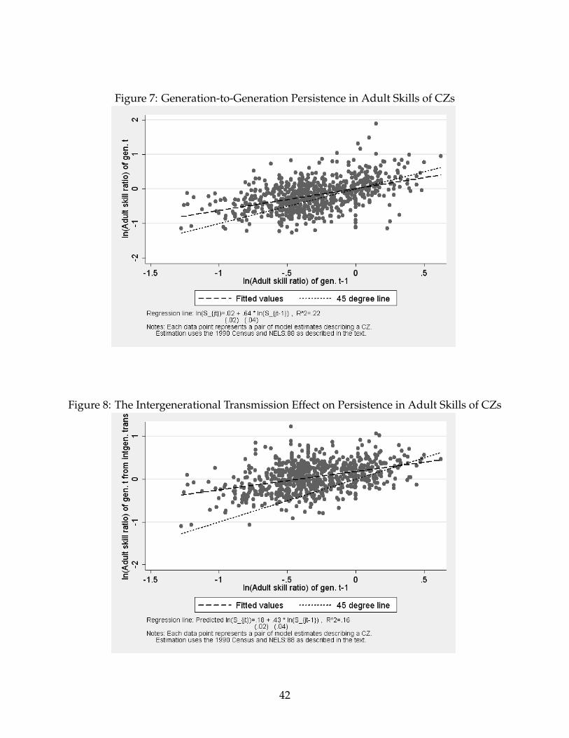
Figure 7: Generation-to-Generation Persistence in Adult Skills of CZs

Figure 8: The Intergenerational Transmission Effect on Persistence in Adult Skills of CZs

42

Figure 9: The Migration Effect on Persistence in Adult Skills of CZs

Figure 10: Childhood and Adult CZ Location Skills of a Cohort

43

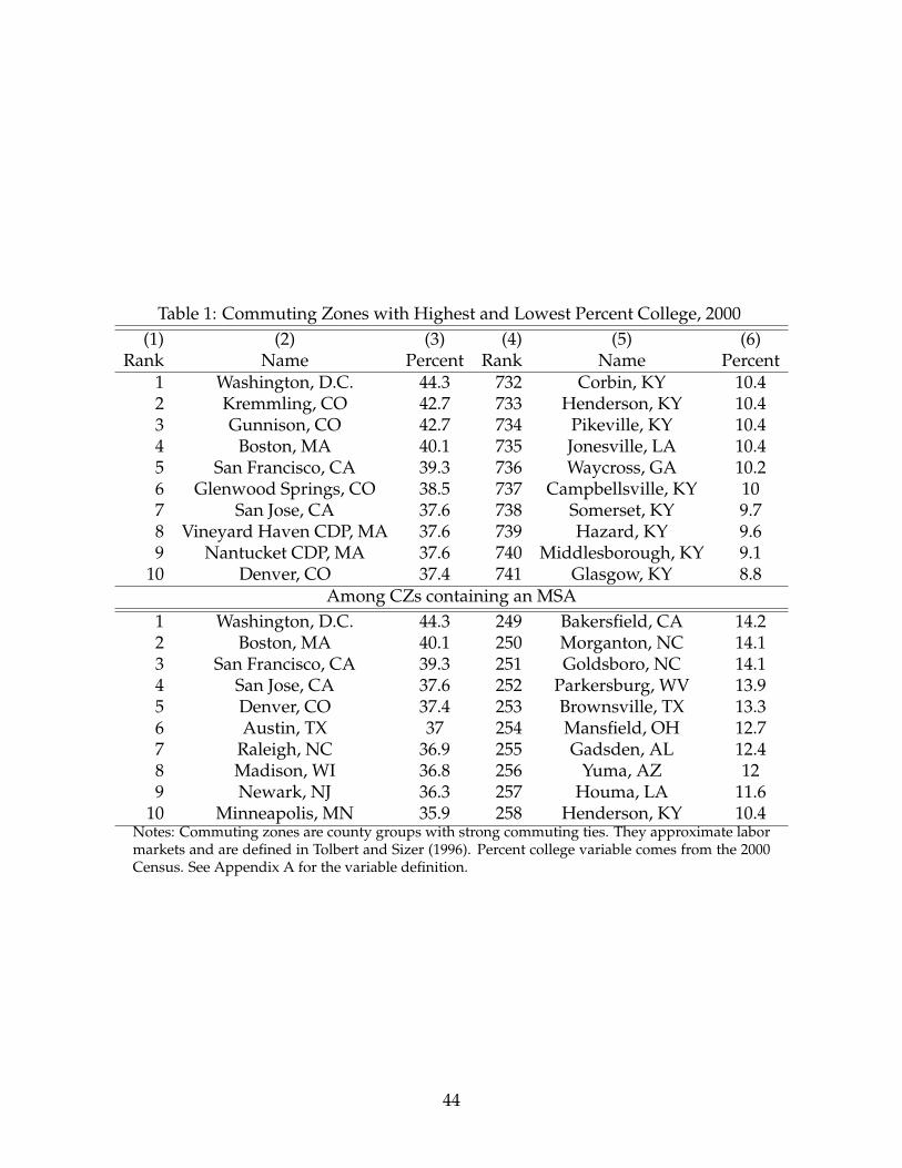
Table 1: Commuting Zones with Highest and Lowest Percent College, 2000(1) (2) (3) (4) (5) (6)

Rank Name Percent Rank Name Percent1 Washington, D.C. 44.3 732 Corbin, KY 10.42 Kremmling, CO 42.7 733 Henderson, KY 10.43 Gunnison, CO 42.7 734 Pikeville, KY 10.44 Boston, MA 40.1 735 Jonesville, LA 10.45 San Francisco, CA 39.3 736 Waycross, GA 10.26 Glenwood Springs, CO 38.5 737 Campbellsville, KY 107 San Jose, CA 37.6 738 Somerset, KY 9.78 Vineyard Haven CDP, MA 37.6 739 Hazard, KY 9.69 Nantucket CDP, MA 37.6 740 Middlesborough, KY 9.1

10 Denver, CO 37.4 741 Glasgow, KY 8.8Among CZs containing an MSA

1 Washington, D.C. 44.3 249 Bakersfield, CA 14.22 Boston, MA 40.1 250 Morganton, NC 14.13 San Francisco, CA 39.3 251 Goldsboro, NC 14.14 San Jose, CA 37.6 252 Parkersburg, WV 13.95 Denver, CO 37.4 253 Brownsville, TX 13.36 Austin, TX 37 254 Mansfield, OH 12.77 Raleigh, NC 36.9 255 Gadsden, AL 12.48 Madison, WI 36.8 256 Yuma, AZ 129 Newark, NJ 36.3 257 Houma, LA 11.6

10 Minneapolis, MN 35.9 258 Henderson, KY 10.4Notes: Commuting zones are county groups with strong commuting ties. They approximate labormarkets and are defined in Tolbert and Sizer (1996). Percent college variable comes from the 2000Census. See Appendix A for the variable definition.

44

Table 2: Accounting for Skills across States, Census(1) (2) (3) (4) (5)

Description Variable Mean StDev Skew Min Max

Parent gen. skill ratio Sjt−1 1.03 .26 .25 .56 1.68Child skill ratio Kjt .99 .27 .27 .53 1.63Stayers skill ratio KjtΛjt .71 .24 .71 .38 1.37Adult skill ratio Sjt .96 .29 .67 .49 1.76

Intergenerational factor Kjt/Sjt−1 .98 .23 .82 .48 1.83Native retention factor Λjt .71 .11 -.89 .3 .98In-migration factor Mjt 1.42 .45 3.75 1.05 3.95Total migration factor ΛjtMjt .99 .21 .52 .64 1.47

Notes: Estimates from accounting exercise described in Section 3. Data come fromthe 1980 and 2000 Census.

Table 3: Correlations between Accounting Exercise Characteristics of States, Census(1) (2) (3) (4) (5) (6) (7) (8)Sjt−1 Kjt KjtΛjt Sjt Kjt/Sjt−1 Λjt Mjt ΛjtMjt

Sjt−1 1Kjt .53 1KjtΛjt .545 .851 1Sjt .516 .738 .746 1

Kjt/Sjt−1 -.376 .557 .313 .316 1Λjt .143 .03 .539 .263 -.227 1Mjt -.115 -.109 -.383 .303 .154 -.509 1ΛjtMjt .032 -.26 -.059 .443 -.281 .336 .566 1

Notes: Estimates from accounting exercise described in Section 3. Data come fromthe 1980 and 2000 Census.

45

Table 4: Generation-to-Generation Persistence of Skills across States, Census(1) (2) (3) (4)

Adult skill Intergenerational Migration Adult skillratio transmission effect effect ratio

VARIABLES ln(Sjt) ln(Sjt−1) + ln(

Kjt

Sjt−1

)ln(Sjt−1) + ln(ΛjtMjt) ln(Sjt)

ln(Sjt−1) .647*** .663*** .985***(.135) (.119) (.115)

ln(Kjt) .793***(.104)

Constant -.0823** -.0475 -.0349 -.0449(.035) (.0309) (.0298) (.0291)

Observations 51 51 51 51R-squared 0.321 0.388 0.601 0.545

Notes: ***p<0.01 **p<0.05 *p<0.1. Dependent variable is the column heading. Each column hasresults from a separate regression. Variables are estimates from accounting exercise described inSection 3. Data come from the 1980 and 2000 Census.

Table 5: Characteristics of the 741 Commuting Zones, 2000(1) (2) (3) (4)

Variable Mean StDev Min Max

South .394 .489 0 1Midwest .34 .474 0 1West .209 .407 0 1Northeast .057 .231 0 1Coastal .124 .33 0 1Annual snow (in.) 22.3 24.7 0 157.3Avg January temp (degF) 31.8 12.3 -23 70.4Avg July temp (degF) 74.5 6.4 42.3 91.6Percent college degree 20 6 8.8 44.3Percent unemployed 5.6 2.1 2.5 16Avg weekly wage 661 94 504 1160Percent manufacturing 15.9 8.2 2.4 44.4Wage tax 43.6 1.8 40.8 46.7Capital tax 23.9 1.8 21.2 27.1Higher ed subsidy 2.7 1.1 .4 5.8College enrollment 14648 38924 0 657298Population 379787 1047226 1193 16393360Notes: Commuting zones are county groups with strong commuting ties.They approximate labor markets and are defined in Tolbert and Sizer(1996). See Section 5 for a description of data sources. Appendix A hasadditional information.

46

Table 6: Characteristics of Respondents, by Move Status, NELS:88(1) (2) (3) (4) (5) (6)

All Movers Stayers[N = 11079] [N = 3833] [N = 7246]

[Rate = .346] [Rate = .654]

Variable Mean SE Mean SE Mean SE

HS Dropout .068 .007 .057 .013 .074 .008College Grad .293 .008 .444 .014 .217 .009Test Index 10.026 .001 10.039 .001 10.019 .001Parents Ed 13.847 .04 14.504 .06 13.514 .052Parents Income 41627 596 49358 1034 37715 701Predict Log Earnings 10.187 .006 10.269 .008 10.146 .007Female .504 .011 .491 .015 .51 .014Asian .035 .003 .034 .005 .035 .004Hispanic .105 .006 .068 .008 .123 .009Black .132 .011 .075 .009 .16 .016White .714 .011 .814 .012 .664 .015Married .47 .011 .48 .015 .466 .014Any Kids .407 .011 .278 .014 .472 .014Notes: The test index is a log earnings prediction using respondent 8th grade mathand verbal test scores as predictors. This is described in Section 5. Parents Ed isthe higher of parents’ years of schooling. Predict Log Earnings is a predictionof log annual earnings for a person with the respondent’s characteristics from aregression with full-time workers in the NELS:88. Moving is defined as living in aCZ at age 26 other than the CZ of a respondent’s 8th grade school.

47

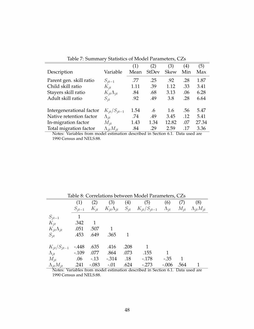
Table 7: Summary Statistics of Model Parameters, CZs(1) (2) (3) (4) (5)

Description Variable Mean StDev Skew Min Max

Parent gen. skill ratio Sjt−1 .77 .25 .92 .28 1.87Child skill ratio Kjt 1.11 .39 1.12 .33 3.41Stayers skill ratio KjtΛjt .84 .68 3.13 .06 6.28Adult skill ratio Sjt .92 .49 3.8 .28 6.64

Intergenerational factor Kjt/Sjt−1 1.54 .6 1.6 .56 5.47Native retention factor Λjt .74 .49 3.45 .12 5.41In-migration factor Mjt 1.43 1.34 12.82 .07 27.34Total migration factor ΛjtMjt .84 .29 2.59 .17 3.36

Notes: Variables from model estimation described in Section 6.1. Data used are1990 Census and NELS:88.

Table 8: Correlations between Model Parameters, CZs(1) (2) (3) (4) (5) (6) (7) (8)Sjt−1 Kjt KjtΛjt Sjt Kjt/Sjt−1 Λjt Mjt ΛjtMjt

Sjt−1 1Kjt .342 1KjtΛjt .051 .507 1Sjt .453 .649 .365 1

Kjt/Sjt−1 -.448 .635 .416 .208 1Λjt -.109 .077 .864 .073 .155 1Mjt .06 -.13 -.314 .18 -.178 -.35 1ΛjtMjt .241 -.083 -.01 .624 -.273 -.006 .564 1

Notes: Variables from model estimation described in Section 6.1. Data used are1990 Census and NELS:88.

48

Table 9: Generation-to-Generation Persistence of Skills across CZs, NELS:88(1) (2) (3) (4)

Adult skill Intergenerational Migration Adult skillratio transmission effect effect ratio

VARIABLES ln(Sjt) ln(Sjt−1) + ln(

Kjt

Sjt−1

)ln(Sjt−1) + ln(ΛjtMjt) ln(Sjt)

ln(Sjt−1) .635*** .432*** 1.2***(.0445) (.0369) (.0363)

ln(Kjt) .858***(.0335)

Constant .016 .184*** -.168*** -.225***(.0198) (.0164) (.0161) (.0116)

Observations 741 741 741 741R-squared 0.216 0.156 0.598 0.470

Notes: ***p<0.01 **p<0.05 *p<0.1. Dependent variable is the column heading. Each column hasresults from a separate regression. Variables are from model estimation described in Section 6.1.Data used are 1990 Census and NELS:88.

49

Table 10: Correlates with the Skill Content of Migration, ln(ΛjtMjt)

VARIABLES (1) (2) (3) (4) (5) (6) (7) (8)ln(K jt) -.142*** .00127 .0753* -.00216 .0219 .0204

(.0335) (.0351) (.0389) (.0363) (.0375) (.0375)South -.167*** -.167*** -.293*** -.303*** -.286*** -.302*** -.302***

(.0273) (.0282) (.038) (.0334) (.0334) (.0368) (.0368)Midwest -.288*** -.288*** -.373*** -.359*** -.354*** -.368*** -.365***

(.0282) (.0291) (.0371) (.0326) (.0328) (.0358) (.0353)Northeast -.274*** -.275*** -.285*** -.155*** -.152*** -.167*** -.164***

(.0475) (.0483) (.0512) (.0459) (.0467) (.0488) (.0485)Coastal -.042 -.0418 -.000512 .00611 .0182 .0252 .0245

(.0324) (.0328) (.0361) (.0317) (.0316) (.0324) (.0323)Small town -.551*** -.551*** -.51*** -.48*** -.471*** -.463*** -.463***

(.0466) (.0467) (.047) (.0418) (.0416) (.0424) (.0423)Small urban -.305*** -.305*** -.262*** -.297*** -.289*** -.289*** -.291***

(.0441) (.0442) (.0441) (.0388) (.0385) (.0385) (.0382)Larger urban -.201*** -.201*** -.168*** -.237*** -.23*** -.231*** -.234***

(.0481) (.0482) (.0475) (.0421) (.0418) (.0419) (.0417)Small metro -.271*** -.271*** -.241*** -.276*** -.271*** -.273*** -.274***

(.0467) (.0467) (.046) (.0405) (.0402) (.0403) (.0402)Medium metro -.121** -.121** -.103** -.141*** -.135*** -.135*** -.136***

(.0485) (.0485) (.0476) (.0419) (.0416) (.0416) (.0415)Jan Temp (degF) -.00197 -.0072*** -.00649*** -.00661*** -.0069***

(.00182) (.00164) (.00164) (.00164) (.00155)July Temp (degF) .00905** .00932*** .0103*** .011*** .011***

(.00367) (.00323) (.00322) (.0033) (.00329)Ann. Snow (in) -.00207*** -.00108* -.000807 -.0007 -.00068

(.000645) (.000571) (.000572) (.000582) (.00058)College enroll/Pop 1.12*** 1.1*** 1.13*** 1.18***

(.242) (.241) (.243) (.228)Ln(College subsidy) .35*** .35*** .351*** .352***

(.025) (.0271) (.0272) (.0269)Wage tax .0336*** .0331*** .0333***

(.0126) (.0126) (.0126)Capital tax -.0181 -.0187 -.0197

(.0127) (.0127) (.0126)% Manufacturing .00134 .00137

(.00132) (.00132)Constant -.225*** .239*** .239*** -.29 -.499** -1.65*** -1.68*** -1.65***

(.0116) (.0463) (.0464) (.248) (.218) (.393) (.394) (.392)Observations 741 741 741 741 741 741 741 741R-squared 0.024 0.305 0.305 0.338 0.491 0.501 0.502 0.501

Notes: ***p<0.01 **p<0.05 *p<0.1. Each column has results from a separate OLS model with CZs as obser-vations. Dependent variable is the model estimate of a CZ’s skill migration parameter (ln(ΛjtMjt)). Majormetro area is the omitted CZ size category. West is the omitted CZ region. ln(Kjt) is a model estimate ofthe CZ’s log child skill ratio. See text for definitions of other variables.

50

Table 11: Correlates with the Intergenerational Transmission Effect on Local Skill,ln(Kj(Sjt−1))− ln(Sjt−1)

VARIABLES (1) (2) (3) (4) (5) (6) (7) (8)ln(Sjt−1) -.568*** -.423*** -.552*** -.606*** -.607*** -.56***

(.0369) (.0394) (.0382) (.0372) (.0358) (.0368)South .162*** .0108 .137*** .119*** .0941*** .0396 .108***

(.0273) (.029) (.0342) (.0329) (.0318) (.0337) (.0383)Midwest .394*** .315*** .247*** .229*** .247*** .195*** .251***

(.0281) (.0271) (.0328) (.0315) (.0305) (.0322) (.0368)Northeast .347*** .301*** .186*** .181*** .239*** .186*** .233***

(.0474) (.0443) (.0451) (.044) (.0431) (.0441) (.0505)Coastal -.233*** -.191*** -.109*** -.0837*** -.0931*** -.0697** -.114***

(.0323) (.0303) (.0319) (.0307) (.0294) (.0295) (.0337)Small town .523*** .337*** .172*** .201*** .191*** .249*** .553***

(.0465) (.0466) (.0455) (.0437) (.042) (.0433) (.0441)Small urban .469*** .249*** .119*** .0984** .0996** .127*** .445***

(.044) (.0458) (.044) (.0422) (.0406) (.0405) (.0398)Larger urban .4*** .226*** .126*** .0694 .0792* .0942** .352***

(.048) (.0475) (.0448) (.0435) (.0418) (.0414) (.0434)Small metro .338*** .213*** .121*** .0829** .0799** .0896** .278***

(.0465) (.0448) (.0422) (.0407) (.0389) (.0385) (.0418)Medium metro .142*** .0792* .053 .024 .0238 .0324 .131***

(.0484) (.0454) (.042) (.0404) (.0387) (.0382) (.0433)Jan Temp (degF) -.0108*** -.0116*** -.012*** -.0121*** -.0095***

(.00154) (.0015) (.00144) (.00142) (.00162)July Temp (degF) -.00165 -.000255 -.00141 .00181 .0062*

(.00321) (.00308) (.00295) (.003) (.00343)Ann. Snow (in) .000772 .000935* .000319 .000696 .000315

(.000565) (.000544) (.000527) (.000527) (.000604)College enroll/Pop 1.8*** 1.78*** 1.85*** 1.4***

(.221) (.211) (.209) (.238)Ln(College subsidy) .0245 .0937*** .0969*** .103***

(.0238) (.0247) (.0244) (.028)Wage tax .0223* .0216* .0391***

(.0116) (.0115) (.0131)Capital tax -.0574*** -.0611*** -.0794***

(.0116) (.0115) (.0131)% Manufacturing .00562*** .011***

(.00124) (.00137)Constant .184*** -.204*** -.0945** .387* .233 .683* .491 -.417

(.0164) (.0462) (.0442) (.217) (.209) (.362) (.36) (.408)Observations 741 741 741 741 741 741 741 741R-squared 0.243 0.473 0.545 0.615 0.648 0.679 0.688 0.588Notes: ***p<0.01 **p<0.05 *p<0.1. Each column has results from a separate OLS model with CZs as ob-servations. Dependent variable is the model estimate of a CZ’s skill gains through intergenerational trans-mission (ln(Kj(Sjt−1)) − ln(Sjt−1)). Major metro area is the omitted CZ size category. West is the omittedCZ region. ln(Sjt−1) is a model estimate of the CZ’s log skill ratio in the previous generation. See text fordefinitions of other variables.

51

Table 12: Correlates with the Skill Content of Native Leaving and Staying, ln(Λjt)

VARIABLES (1) (2) (3) (4) (5) (6) (7) (8)ln(Kjt) .132** .0819 .222*** .332*** .335*** .32***

(.0514) (.0589) (.0657) (.0687) (.0716) (.0704)South -.0884* -.0724 -.278*** -.275*** -.282*** -.433*** -.438***

(.0459) (.0473) (.0641) (.0632) (.0639) (.069) (.07)Midwest -.0661 -.0831* -.171*** -.178*** -.19*** -.33*** -.282***

(.0473) (.0488) (.0626) (.0618) (.0627) (.0671) (.0672)Northeast -.126 -.146* -.182** -.193** -.212** -.352*** -.305***

(.0799) (.081) (.0864) (.0869) (.0893) (.0916) (.0922)Coastal -.427*** -.416*** -.393*** -.41*** -.416*** -.348*** -.359***

(.0544) (.055) (.0609) (.0601) (.0605) (.0607) (.0615)Small town -.145* -.152* -.0546 -.117 -.121 -.0421 -.0393

(.0783) (.0784) (.0793) (.0793) (.0794) (.0795) (.0805)Small urban -.0733 -.0691 .00235 .00348 -.00106 -.0018 -.0412

(.0742) (.0742) (.0743) (.0734) (.0736) (.0723) (.0727)Larger urban -.473*** -.472*** -.422*** -.377*** -.383*** -.401*** -.436***

(.0809) (.0808) (.0801) (.0798) (.0799) (.0786) (.0792)Small metro -.244*** -.248*** -.201** -.175** -.176** -.193** -.211***

(.0784) (.0784) (.0776) (.0768) (.0768) (.0755) (.0764)Medium metro -.176** -.175** -.161** -.135* -.139* -.139* -.153*

(.0815) (.0814) (.0802) (.0794) (.0794) (.078) (.079)Jan Temp (degF) .00473 .00659** .00646** .00533* .000784

(.00306) (.0031) (.00313) (.00308) (.00295)July Temp (degF) .0181*** .0165*** .0161*** .0232*** .0227***

(.0062) (.00612) (.00614) (.00618) (.00626)Ann. Snow (in) .000979 .000767 .000698 .00174 .00206*

(.00109) (.00108) (.00109) (.00109) (.0011)College enroll/Pop -2.19*** -2.21*** -1.9*** -1.19***

(.458) (.46) (.456) (.434)Ln(College subsidy) -.0121 -.0311 -.0231 .00649

(.0474) (.0518) (.0509) (.0512)Wage tax -.0319 -.0371 -.0346

(.024) (.0236) (.0239)Capital tax .0297 .0236 .00865

(.0242) (.0238) (.0239)% Manufacturing .013*** .0134***

(.00247) (.0025)Constant -.435*** -.132* -.136* -1.61*** -1.46*** -.714 -.985 -.6

(.0179) (.0778) (.0778) (.418) (.414) (.751) (.74) (.745)Observations 741 741 741 741 741 741 741 741R-squared 0.009 0.154 0.156 0.188 0.212 0.214 0.243 0.222Notes: ***p<0.01 **p<0.05 *p<0.1. Each column has results from a separate OLS model with CZs as ob-servations. Dependent variable is the model estimate of a CZ’s native skill retention parameter (ln(Λjt)).Major metro area is the omitted CZ size category. West is the omitted CZ region. ln(Kjt) is a model estimateof the CZ’s log child skill ratio. See text for definitions of other variables.

52

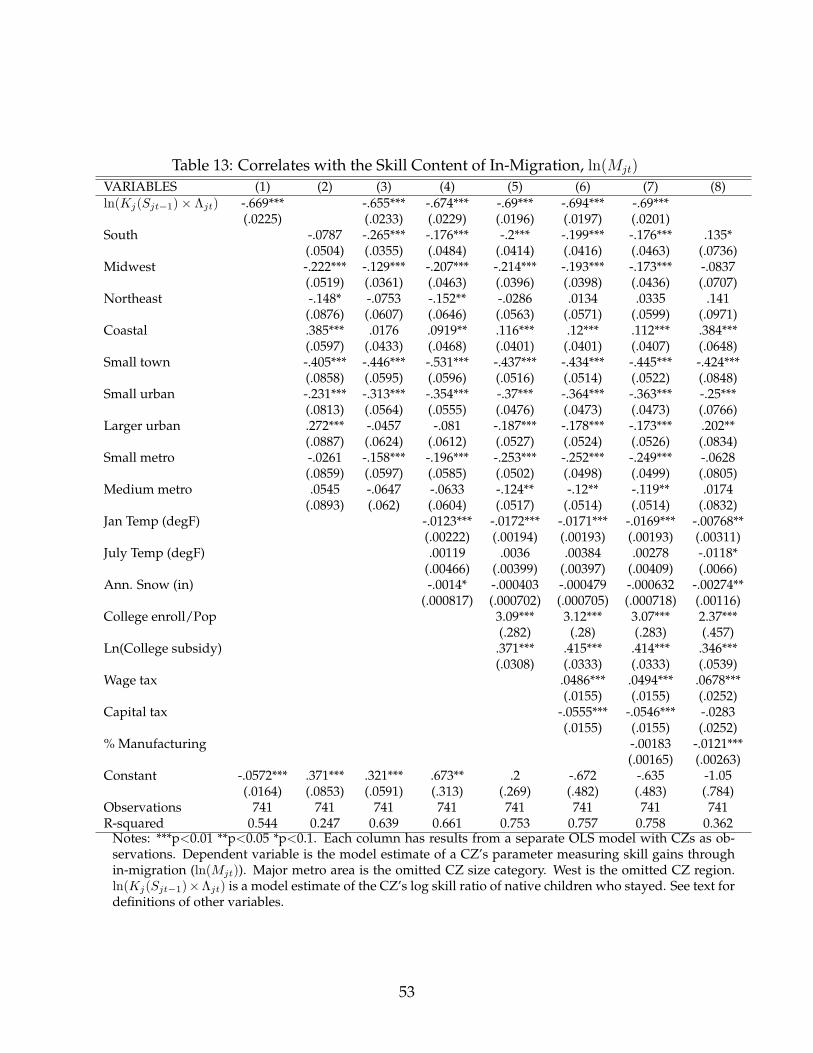
Table 13: Correlates with the Skill Content of In-Migration, ln(Mjt)

VARIABLES (1) (2) (3) (4) (5) (6) (7) (8)ln(Kj(Sjt−1)× Λjt) -.669*** -.655*** -.674*** -.69*** -.694*** -.69***

(.0225) (.0233) (.0229) (.0196) (.0197) (.0201)South -.0787 -.265*** -.176*** -.2*** -.199*** -.176*** .135*

(.0504) (.0355) (.0484) (.0414) (.0416) (.0463) (.0736)Midwest -.222*** -.129*** -.207*** -.214*** -.193*** -.173*** -.0837

(.0519) (.0361) (.0463) (.0396) (.0398) (.0436) (.0707)Northeast -.148* -.0753 -.152** -.0286 .0134 .0335 .141

(.0876) (.0607) (.0646) (.0563) (.0571) (.0599) (.0971)Coastal .385*** .0176 .0919** .116*** .12*** .112*** .384***

(.0597) (.0433) (.0468) (.0401) (.0401) (.0407) (.0648)Small town -.405*** -.446*** -.531*** -.437*** -.434*** -.445*** -.424***

(.0858) (.0595) (.0596) (.0516) (.0514) (.0522) (.0848)Small urban -.231*** -.313*** -.354*** -.37*** -.364*** -.363*** -.25***

(.0813) (.0564) (.0555) (.0476) (.0473) (.0473) (.0766)Larger urban .272*** -.0457 -.081 -.187*** -.178*** -.173*** .202**

(.0887) (.0624) (.0612) (.0527) (.0524) (.0526) (.0834)Small metro -.0261 -.158*** -.196*** -.253*** -.252*** -.249*** -.0628

(.0859) (.0597) (.0585) (.0502) (.0498) (.0499) (.0805)Medium metro .0545 -.0647 -.0633 -.124** -.12** -.119** .0174

(.0893) (.062) (.0604) (.0517) (.0514) (.0514) (.0832)Jan Temp (degF) -.0123*** -.0172*** -.0171*** -.0169*** -.00768**

(.00222) (.00194) (.00193) (.00193) (.00311)July Temp (degF) .00119 .0036 .00384 .00278 -.0118*

(.00466) (.00399) (.00397) (.00409) (.0066)Ann. Snow (in) -.0014* -.000403 -.000479 -.000632 -.00274**

(.000817) (.000702) (.000705) (.000718) (.00116)College enroll/Pop 3.09*** 3.12*** 3.07*** 2.37***

(.282) (.28) (.283) (.457)Ln(College subsidy) .371*** .415*** .414*** .346***

(.0308) (.0333) (.0333) (.0539)Wage tax .0486*** .0494*** .0678***

(.0155) (.0155) (.0252)Capital tax -.0555*** -.0546*** -.0283

(.0155) (.0155) (.0252)% Manufacturing -.00183 -.0121***

(.00165) (.00263)Constant -.0572*** .371*** .321*** .673** .2 -.672 -.635 -1.05

(.0164) (.0853) (.0591) (.313) (.269) (.482) (.483) (.784)Observations 741 741 741 741 741 741 741 741R-squared 0.544 0.247 0.639 0.661 0.753 0.757 0.758 0.362

Notes: ***p<0.01 **p<0.05 *p<0.1. Each column has results from a separate OLS model with CZs as ob-servations. Dependent variable is the model estimate of a CZ’s parameter measuring skill gains throughin-migration (ln(Mjt)). Major metro area is the omitted CZ size category. West is the omitted CZ region.ln(Kj(Sjt−1)×Λjt) is a model estimate of the CZ’s log skill ratio of native children who stayed. See text fordefinitions of other variables.

53

Table 14: Correlates with the Local Native Children Skill Ratio, ln(Kj(Sjt−1))

VARIABLES (1) (2) (3) (4) (5) (6) (7) (8)ln(Sjt−1) .432*** .577*** .448*** .394*** .393*** .44***

(.0369) (.0394) (.0382) (.0372) (.0358) (.0368)South -.195*** .0108 .137*** .119*** .0941*** .0396 -.0141

(.0288) (.029) (.0342) (.0329) (.0318) (.0337) (.0365)Midwest .208*** .315*** .247*** .229*** .247*** .195*** .152***

(.0297) (.0271) (.0328) (.0315) (.0305) (.0322) (.035)Northeast .237*** .301*** .186*** .181*** .239*** .186*** .149***

(.0501) (.0443) (.0451) (.044) (.0431) (.0441) (.0481)Coastal -.134*** -.191*** -.109*** -.0837*** -.0931*** -.0697** -.0349

(.0341) (.0303) (.0319) (.0307) (.0294) (.0295) (.0321)Small town .0838* .337*** .172*** .201*** .191*** .249*** .0089

(.0491) (.0466) (.0455) (.0437) (.042) (.0433) (.042)Small urban -.0517 .249*** .119*** .0984** .0996** .127*** -.123***

(.0465) (.0458) (.044) (.0422) (.0406) (.0405) (.0379)Larger urban -.0119 .226*** .126*** .0694 .0792* .0942** -.108***

(.0507) (.0475) (.0448) (.0435) (.0418) (.0414) (.0413)Small metro .0433 .213*** .121*** .0829** .0799** .0896** -.0587

(.0492) (.0448) (.0422) (.0407) (.0389) (.0385) (.0399)Medium metro -.00638 .0792* .053 .024 .0238 .0324 -.0448

(.0511) (.0454) (.042) (.0404) (.0387) (.0382) (.0412)Jan Temp (degF) -.0108*** -.0116*** -.012*** -.0121*** -.0142***

(.00154) (.0015) (.00144) (.00142) (.00154)July Temp (degF) -.00165 -.000255 -.00141 .00181 -.00163

(.00321) (.00308) (.00295) (.003) (.00327)Ann. Snow (in) .000772 .000935* .000319 .000696 .000995*

(.000565) (.000544) (.000527) (.000527) (.000575)College enroll/Pop 1.8*** 1.78*** 1.85*** 2.21***

(.221) (.211) (.209) (.227)Ln(College subsidy) .0245 .0937*** .0969*** .0923***

(.0238) (.0247) (.0244) (.0267)Wage tax .0223* .0216* .00792

(.0116) (.0115) (.0125)Capital tax -.0574*** -.0611*** -.0467***

(.0116) (.0115) (.0125)% Manufacturing .00562*** .0014

(.00124) (.0013)Constant .184*** .0553 -.0945** .387* .233 .683* .491 1.21***

(.0164) (.0488) (.0442) (.217) (.209) (.362) (.36) (.388)Observations 741 741 741 741 741 741 741 741R-squared 0.156 0.344 0.493 0.571 0.607 0.642 0.652 0.583Notes: ***p<0.01 **p<0.05 *p<0.1. Each column has results from a separate OLS model with CZs asobservations. Dependent variable is the model estimate of a CZ’s native children skill ratio parameter(ln(Kj(Sjt−1))). Major metro area is the omitted CZ size category. West is the omitted CZ region. ln(Sjt−1)is a model estimate of the CZ’s log skill ratio of the previous generation. See text for definitions of othervariables.

54

Table 15: Correlates with the Local Adult Skill Ratio, ln(Sjt)

VARIABLES (1) (2) (3) (4) (5) (6) (7) (8)ln(Sjt−1) .635*** .615*** .552*** .457*** .471*** .538***

(.0445) (.0575) (.0592) (.0531) (.0526) (.0542)South -.363*** -.143*** -.13** -.171*** -.174*** -.251*** -.316***

(.0398) (.0423) (.053) (.047) (.0468) (.0496) (.0523)Midwest -.0803* .0343 -.0937* -.118*** -.0869* -.16*** -.214***

(.0409) (.0396) (.0507) (.045) (.0449) (.0475) (.0502)Northeast -.037 .0303 -.0722 .0372 .105* .0303 -.0148

(.0691) (.0646) (.0698) (.0629) (.0634) (.0649) (.069)Coastal -.176*** -.237*** -.127** -.0863** -.086** -.053 -.0104

(.0471) (.0442) (.0493) (.0438) (.0432) (.0434) (.046)Small town -.467*** -.197*** -.289*** -.249*** -.242*** -.161** -.454***

(.0677) (.0679) (.0704) (.0624) (.0617) (.0638) (.0602)Small urban -.356*** -.0361 -.0936 -.163*** -.147** -.109* -.414***

(.0642) (.0668) (.0681) (.0603) (.0597) (.0596) (.0544)Larger urban -.213*** .0405 -.000996 -.138** -.116* -.0945 -.342***

(.07) (.0693) (.0694) (.0622) (.0615) (.061) (.0593)Small metro -.227*** -.0463 -.0881 -.171*** -.165*** -.152*** -.333***

(.0678) (.0653) (.0653) (.0581) (.0573) (.0567) (.0572)Medium metro -.127* -.0362 -.0353 -.106* -.0984* -.0862 -.181***

(.0705) (.0662) (.065) (.0577) (.0569) (.0563) (.0591)Jan Temp (degF) -.0132*** -.0184*** -.0184*** -.0186*** -.0211***

(.00238) (.00214) (.00211) (.00209) (.00221)July Temp (degF) .00749 .00919** .00899** .0135*** .00932**

(.00497) (.0044) (.00434) (.00442) (.00469)Ann. Snow (in) -.00135 -.000246 -.000582 -.0000502 .000316

(.000875) (.000778) (.000775) (.000776) (.000825)College enroll/Pop 2.85*** 2.85*** 2.95*** 3.39***

(.316) (.311) (.308) (.325)Ln(College subsidy) .374*** .446*** .45*** .445***

(.0341) (.0364) (.036) (.0383)Wage tax .0589*** .0579*** .0412**

(.0171) (.0169) (.0179)Capital tax -.0788*** -.084*** -.0664***

(.0171) (.0169) (.0179)% Manufacturing .00793*** .00277

(.00183) (.00187)Constant .016 .295*** .135** .0853 -.298 -1.05** -1.32** -.447

(.0198) (.0673) (.0644) (.336) (.298) (.533) (.53) (.557)Observations 741 741 741 741 741 741 741 741R-squared 0.216 0.203 0.311 0.343 0.488 0.506 0.518 0.452Notes: ***p<0.01 **p<0.05 *p<0.1. Each column has results from a separate OLS model with CZs as ob-servations. Dependent variable is the model estimate of a CZ’s skill ratio parameter (ln(Sjt)). Major metroarea is the omitted CZ size category. West is the omitted CZ region. ln(Sjt−1) is a model estimate of theCZ’s log skill ratio in the previous generation. See text for definitions of other variables.

55

A Data Appendix

A.1 Commuting zones and their characteristics

Tolbert and Sizer (1996) describe the procedure they used to create the CZ classification.

CZs were defined using confidential 1990 Census journey-to-work data. They are clusters

of counties or county equivalents (boroughs, parishes, Census areas, and independent

cities) with particularly strong commuting ties. There are 741 of them. CZs cross state

lines and cover the entire United States (unlike alternative geographic units like MSAs).

Tolbert and Sizer (1996) provide some useful characterizations of CZs. They categorize

CZs into four regions of the U.S.: Northeast, South, Midwest, and West. They also classify

CZs as falling into one of six categories: small town, small urban, large urban, small

metro, medium metro, and major metro. These are descriptions of the largest population

center in each CZ. Small towns have fewer than 5,000 residents, small urban centers have

between 5,000 and 20,000, and larger urban centers have at least 20,000 but no MSAs in

the CZ. The remaining three categories are CZs with at least one MSA in their territory.

They are classified according to the size of the largest MSA, where small metro centers

have fewer than 250,000 residents, medium metro centers have between 250,000 and 1

million, and major metro centers have more than 1 million. These population figures

refer to 1990.

I obtain additional characteristics of CZs from the 5 percent samples of the 1990 and

2000 Census (Ruggles et al. 2004). I follow Autor and Dorn (2007) in matching Census

data to CZs. The least aggregated geographic unit identifiable in the 1990 and 2000 5

percent samples from IPUMS is the public use microdata area (PUMA). These are county

clusters and are on average smaller than CZs. However, there exist PUMAs that overlap

CZ boundaries. In order to match the two classifications, I weight average characteristics

of PUMAs according to 2000 county populations when attributing those characteristics

to a CZ. More specifically, I break down CZs into their individual counties. I assign to

each county the average characteristic in the county’s PUMA. I then create the CZ average

56

characteristic by taking the weighted average of county characteristics, where the weights

are the proportion of CZ residents residing in each county.

The CZ characteristics derived from the 2000 Census are the following:

• Percent with at least a bachelor’s degree. The population here is restricted to those

at least 24 years old and no older than 64.

• Average weekly wage. The population here is restricted to those currently em-

ployed and at least 16 years old and no older than 64. I weight by a labor supply

variable, which is weeks worked in the previous year times usual weekly hours. For

those with missing values of these variables, I impute labor supply as the average in

their education-occupation cell, or just their education cell if the previous includes

only themselves. I take wage and salary income from the previous year as the base-

line earnings measure. I multiply top-coded ($175,000 in 2000) values by 1.5. The

weekly wage is the resulting number divided by weeks worked.

• Percent employed in the manufacturing industry. These are workers with 2000 Cen-

sus industry codes between 107 and 399, inclusive. The population includes only

those working positive hours in the previous year.

All samples are restricted to include only non-institutionalized residents. I also create a

similar data set from the 1990 Census, using the same methods and definitions as much

as possible.

I assign a latitude and longitude to each CZ. I acquire latitude and longitude of ZIP

code tabulation areas (ZCTAs) from the U.S. Census Bureau. These correspond roughly

with zip codes. I then assign zip codes to CZs, using a zip code file purchased from

ZipInfo.com and counties as the merging variable. I assign to each CZ the latitude that

is the midpoint between the minimum and maximum latitudes of zip codes in that CZ. I

assign CZ longitudes similarly.

I use these latitudes and longitudes to calculate distances between CZs. The distance

measure I use is the great circle distance between coordinates, in kilometers.

57

A.2 NELS:88

The procedure used to match NELS:88 respondents to CZ of residence uses zip code vari-

ables in the restricted-use version of the data. I match zip codes to U.S. counties using

a commercial crosswalk (ZipInfo.com). Since CZs are collections of counties, it is then

straightforward to identify the respondent’s CZ. I assign the zip code of the 8th grade

school as the origin of the student and the zip code of residence at the final follow-up

(2000) as the final destination. For some respondents, I am not able to identify the CZ due

to missing data. Tables A.1 and A.2 compare characteristics of respondents for which I do

and do not have CZ identified. I drop respondents with missing CZ from the analysis.

Table A.3 indicates that post-secondary schooling still affects the choices of a signifi-

cant number of NELS:88 respondents in the final follow-up (2000). Twenty-two percent of

respondents were attending classes at either an academic or vocational school at the final

follow-up. Five percent were attending school and not working at all. The cohort had

not all moved on from the school attendance phase of life, and this is a weakness for the

purpose of estimating geographic skill distributions from the model. I plan to estimate

the model with NLSY79 data, where final observed location is later in each respondent’s

life.

58

Table A.1: Characteristics of Respondents, by Base Year Location Data Status(1) (2) (3) (4)

CZ identified CZ not identified[N = 11145] [N = 239]

Variable Mean SE Mean SE

HS Dropout .068 .007 .08 .043College Grad .294 .008 .254 .042Test Index 10.026 .001 10.03 .004Parents Ed 13.851 .04 13.489 .412Parents Income 41685 595 41466 4113Predict Log Earnings 10.188 .006 10.194 .025Female .503 .011 .493 .065Asian .035 .003 .033 .01Hispanic .104 .006 .152 .044Black .131 .011 .025 .009White .715 .011 .782 .047Full-time Work 2000 .594 .01 .606 .061Married .471 .01 .42 .063Any Kids .407 .011 .357 .062

Table A.2: Characteristics of Respondents, by Final Follow-up (2000) Location Data Status(1) (2) (3) (4)

CZ identified CZ not identified[N = 11314] [N = 70]

Variable Mean SE Mean SE

HS Dropout .068 .007 .021 .016College Grad .293 .008 .467 .106Test Index 10.026 .001 10.037 .01Parents Ed 13.839 .04 14.549 .293Parents Income 41606 590 53121 8789Predict Log Earnings 10.187 .006 10.327 .051Female .504 .011 .336 .087Asian .035 .003 .028 .013Hispanic .106 .006 .029 .014Black .129 .011 .078 .037White .716 .011 .859 .046Full-time Work 2000 .594 .01 .66 .087Married .469 .01 .615 .099Any Kids .406 .011 .426 .117

59

Table A.3: School Attendance at Final Follow-Up, NELS:88(1) (2)N Proportion

Total respondents 11079 1In school (final follow-up) 2407 .22In school and PT work 1346 .12In school and FT work 689 .06In school and no work 527 .05

B Results appendix

Table B.1: Probits for Skill Level of Child

(1) (2) (3) (4)Low Medium-Low Medium-High High

Parent low skill .163*** .0507** -.0721*** -.167***(.0286) (.0231) (.0188) (.0141)

Parent medium-low skill .0473* .0308 -.018 -.0854***(.025) (.0246) (.0225) (.017)

Parent high skill -.178*** -.0576*** .0202 .166***(.0174) (.0202) (.0194) (.0194)

Jan Temp (degF) .00186 .0014 -.00416** .000668(.00235) (.00262) (.00194) (.00186)

July Temp (degF) -.00453 .00341 .000384 .000763(.00773) (.00481) (.00476) (.00422)

Ann. Snow (in) -.00018 -.000268 -.000656 .000809(.00124) (.00102) (.000934) (.000784)

Wage tax -.00697 .0137** -.00203 -.00375(.0102) (.00674) (.00747) (.00605)

Ln(college subsidy) -.00556 -.0514 .0881*** -.0312(.0427) (.0376) (.034) (.0314)

College enroll/Pop .189 -.95 .159 .511(.734) (.675) (.578) (.539)

No local college -.0309 -.0899 .102 .00742(.122) (.0698) (.138) (.0908)

Ln(avg wkly wage) .283 -.205 -.0115 -.109(.303) (.199) (.21) (.172)

% College Grad -.00953 .00707 -.00103 .00414(.00765) (.00539) (.00558) (.00413)

Continued on next page

60

Table B.1 – continued from previous pageLow Medium-Low Medium-High High

% Unemployed -.00489 -.00815 .000401 .0135*(.0128) (.0104) (.00988) (.00816)

% Manufacturing -.00151 -.0015 -.00126 .00469**(.00371) (.00227) (.0024) (.0019)

Ln(population) .00386 .0063 .000214 -.00683(.0245) (.0158) (.0177) (.0154)

ParLow × Jan Temp .000657 -.0067* .00464 .0024(.00333) (.00377) (.003) (.00289)

ParLow × July Temp .0126 -.000469 -.00528 -.0142**(.00979) (.00755) (.00704) (.00694)

ParLow × Snow .000717 -.000154 .000786 -.00137(.00191) (.0017) (.00151) (.00119)

ParLow × Tax .0202 -.00914 -.0154 -.00697(.0126) (.00934) (.0104) (.00945)

ParLow × Ln(col subsidy) .0531 .0455 -.104** -.0329(.0649) (.0555) (.0515) (.0482)

ParLow × Col enroll/Pop. -.501 -.478 .836 1.03(1.04) (.993) (.843) (.76)

ParLow × No college -.0727 .0313 .13 -.0321(.172) (.133) (.156) (.13)

ParLow × Log(wkly wage) .00925 -.214 .0298 .276(.436) (.339) (.317) (.301)

ParLow × College grad .00831 .00421 -.00637 -.0116*(.00951) (.00766) (.00747) (.00659)

ParLow × Unemployed .0123 .0141 -.0121 -.0253**(.0159) (.0143) (.0135) (.0113)

ParLow × Manufacture .0024 -.00171 .00299 -.00315(.0044) (.00336) (.00327) (.00314)

ParLow × Log(pop) -.0264 .00443 .0222 .00124(.0363) (.0264) (.0271) (.0261)

ParMedLow × Jan Temp .00159 -.00281 .00396 -.00301(.00337) (.00342) (.00288) (.00274)

ParMedLow × July Temp .00157 .0137* -.00994 -.00795(.00926) (.00798) (.00768) (.00647)

ParMedLow × Snow -.00071 .00196 -.00143 .000529(.00159) (.00144) (.00134) (.00137)

ParMedLow × Tax .0167 -.0347*** .0132 .00366(.0136) (.013) (.0138) (.0109)

ParMedLow × Ln(col subsidy) -.115* .0959 -.086 .12**(.0604) (.0599) (.0561) (.049)

ParMedLow × Col enroll/Pop. -.678 2.07** -1.27 .069(1.03) (.952) (.91) (.881)

Continued on next page

61

Table B.1 – continued from previous pageLow Medium-Low Medium-High High

ParMedLow × No college -.0227 .0138 -.0638 .0064(.23) (.133) (.172) (.129)

ParMedLow × Log(wkly wage) .0644 .328 -.191 -.225(.402) (.328) (.316) (.263)

ParMedLow × College grad .00661 -.0038 .00429 -.0107(.00982) (.00762) (.00837) (.00689)

ParMedLow × Unemployed .0345** -.00101 .003 -.0518***(.0171) (.0155) (.0135) (.0116)

ParMedLow × Manufacture .00323 -.00195 .00263 -.00402(.00458) (.00312) (.00372) (.00298)

ParMedLow × Log(pop) -.00901 .0065 -.0314 .0441*(.0347) (.0256) (.0278) (.0244)

ParHigh × Jan Temp .00258 -.00545* .0057** -.000976(.0032) (.00326) (.00266) (.0024)

ParHigh × July Temp -.00239 -.00327 -.00843 .00858(.00945) (.00681) (.00652) (.00563)

ParHigh × Snow .0000839 -.000671 .000797 -.000195(.00166) (.00141) (.00122) (.00109)

ParHigh × Tax .0184 -.0161 .00108 .00172(.0125) (.0107) (.01) (.00848)

ParHigh × Ln(col subsidy) .00445 .0598 -.0841* .0206(.0568) (.0585) (.0483) (.0443)

ParHigh × Col enroll/Pop. .239 1.05 .205 -.984(.896) (.918) (.773) (.731)

ParHigh × No college -.0037 .0454 .0586 -.0856(.199) (.157) (.161) (.132)

ParHigh × Log(wkly wage) -.466 .205 -.209 .349(.376) (.317) (.297) (.242)

ParHigh × College grad .00765 -.00958 -.00636 .0038(.00916) (.009) (.00725) (.00611)

ParHigh × Unemployed .0000114 .00248 .00265 -.0107(.0161) (.0151) (.0138) (.0117)

ParHigh × Manufacture .00323 -.000951 -.00261 -.000435(.00445) (.00392) (.00322) (.00284)

ParHigh × Log(pop) .00218 -.00222 .0485* -.0367*(.0307) (.0254) (.0256) (.0216)

Observations 11079 11079 11079 11079Pseudo R2 0.0953 0.0330 0.0237 0.103

***p<0.01 **p<0.05 *p<0.1. Dependent variable equals one if respondent’sskill is column heading skill level. Marginal effects reported. Sampleweights used.

62

Table B.2: Destination CZ Choice Logit, Low Skilled(1) (2) (3)

VARIABLES No interaction Home × Rural Origin ×ln(W̄ ) .667

(.959)Home 13.9***

(4.85)South .816*** -.733 .191

(.296) (.533) (.468)Midwest 1.29*** -1.87*** -.0362

(.327) (.554) (.401)West 1.14* -2.58*** .613

(.619) (.533) (.734)Ocean coast -.52* -.147 .0799

(.276) (.398) (.488)Small town -.408 .671 -.592

(.894) (1.25) (1.49)Small urban .0524 -.469 -.478

(.69) (.828) (1.1)Large urban -.307 .67 -.329

(.544) (.755) (.941)Small metro -.0498 -.0383 -.461

(.572) (.64) (.873)Medium metro .33 -.31 .0602

(.325) (.408) (.673)Jan temp .06*** -.0656*** -.0578**

(.0169) (.0241) (.028)July temp -.0297 -.0646 .134***

(.0269) (.0415) (.0471)Ann. Snow -.00152 -.0275*** .0182*

(.00779) (.00887) (.0101)Wage tax -.0399 .124 .0457

(.0487) (.0783) (.0718)Ln(college subsidy) -.81*** .395 .636*

(.305) (.43) (.362)College enroll/Pop 2.17* -1.22 -7.47*

(1.13) (4.53) (4.22)No college 1.42 -.792 -2.78**

(1.08) (.875) (1.22)% BA .01 -.0635** .00154

(.0143) (.0277) (.0248)% Manufacturing .0134 -.016 -.0167

(.0139) (.0206) (.0253)Ln(population) .816*** -.278 -.315

(.174) (.201) (.219)Distance -.0025***

(.000311)Distance2 2.77e-07***

(4.40e-08)BY CZ Col enroll/Pop × Dest. Ln(pop) .35

(1.32)BY CZ Col enroll/Pop × Dest. Ln(col enroll) -4.97

(37.9)Observations 2515*** p<0.01, ** p<0.05, * p<0.1. Results are from a single logit estimation of destination CZchoice. Columns represent interactions between column heading and row variable. Robuststandard errors in parentheses.

63

Table B.3: Destination CZ Choice Logit, Medium-Low Skilled(1) (2) (3)

VARIABLES No interaction Home × Rural Origin ×ln(W̄ ) -.94

(.858)Home 7.69**

(3.69)South .198 -.213 .763

(.303) (.433) (.477)Midwest .0297 -.403 .48

(.276) (.329) (.496)West 1.3** -1.53*** .653

(.628) (.447) (.798)Ocean coast .347 -.455 -.0186

(.29) (.397) (.43)Small town -.769 1.04 -.679

(.857) (1.45) (1.46)Small urban -.111 -.817 .375

(.499) (.937) (.704)Large urban .312 -.125 -.325

(.517) (.712) (.763)Small metro .0629 -.0499 .0256

(.364) (.552) (.584)Medium metro .267 -.104 .45

(.294) (.415) (.544)Jan temp -.00158 -.0122 -.0453

(.0149) (.0201) (.0301)July temp .0284 -.0113 .0289

(.0246) (.0427) (.0632)Ann. Snow .00764* -.0217** -.0031

(.00445) (.00942) (.00817)Wage tax -.0816** .132** .0501

(.0403) (.0663) (.0524)Ln(college subsidy) .232 -.471 -.323

(.165) (.345) (.309)College enroll/Pop 2.32** 1.47 -.509

(.967) (3.9) (2)No college .15 .343 -.258

(.657) (.941) (.979)% BA .0276* -.0013 -.0071

(.0144) (.0254) (.0256)% Manufacturing -.0129 .0529*** .0271

(.0134) (.0195) (.0192)Ln(population) .909*** -.53*** -.219

(.12) (.175) (.194)Distance -.00236***

(.000268)Distance2 2.69e-07***

(3.29e-08)BY CZ Col enroll/Pop × Dest. Ln(pop) 1.44

(1.26)BY CZ Col enroll/Pop × Dest. Ln(col enroll) -23.1

(31.5)Observations 2724*** p<0.01, ** p<0.05, * p<0.1. Results are from a single logit estimation of destination CZchoice. Columns represent interactions between column heading and row variable. Robuststandard errors in parentheses.

64

Table B.4: Destination CZ Choice Logit, Medium-High Skilled(1) (2) (3)

VARIABLES No interaction Home × Rural Origin ×ln(W̄ ) -1.04

(.716)Home 11.7***

(3.95)South .561*** -.136 1*

(.201) (.425) (.574)Midwest .374* -.298 .75

(.2) (.304) (.547)West 1.93*** -1.3*** -.103

(.335) (.399) (.696)Ocean coast -.113 -.00449 .214

(.246) (.292) (.413)Small town 1.47 1.5 -2.11

(.964) (1.24) (1.37)Small urban .0815 -.208 .321

(.492) (.828) (.867)Large urban -.025 .246 .628

(.409) (.815) (.782)Small metro .0875 -.357 1.2

(.328) (.417) (.779)Medium metro .085 .149 .0273

(.217) (.292) (.416)Jan temp -.00924 -.00501 -.00363

(.0114) (.0192) (.0207)July temp .0275 -.00974 -.0392

(.0215) (.037) (.035)Ann. Snow -.00244 .00167 -.00257

(.00462) (.00633) (.00753)Wage tax -.0839** .0379 .00879

(.0383) (.0674) (.0788)Ln(college subsidy) .424** -.184 -1.26***

(.205) (.372) (.373)College enroll/Pop -4.28* 7.64 .2

(2.38) (5.7) (5.15)No college -1.8** -2.47*** 2.75***

(.816) (.839) (.954)% BA .0558*** -.0904*** -.0258

(.0124) (.0253) (.023)% Manufacturing -.0112 .0445** -.0236

(.0117) (.0175) (.0194)Ln(population) .921*** -.465*** .0763

(.103) (.169) (.175)Distance -.00254***

(.00019)Distance2 2.96e-07***

(2.19e-08)BY CZ Col enroll/Pop × Dest. Ln(pop) 1.44

(1.16)BY CZ Col enroll/Pop × Dest. Ln(col enroll) -27.8

(54.1)Observations 2771*** p<0.01, ** p<0.05, * p<0.1. Results are from a single logit estimation of destination CZchoice. Columns represent interactions between column heading and row variable. Robuststandard errors in parentheses.

65

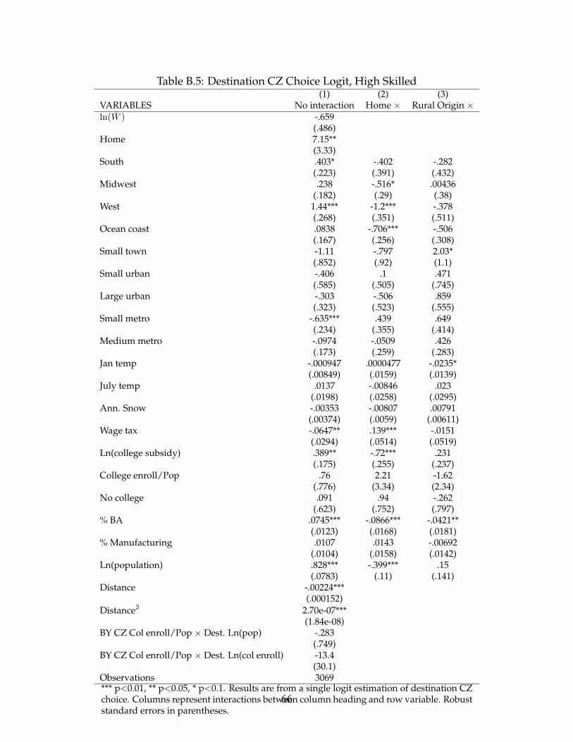
Table B.5: Destination CZ Choice Logit, High Skilled(1) (2) (3)

VARIABLES No interaction Home × Rural Origin ×ln(W̄ ) -.659

(.486)Home 7.15**

(3.33)South .403* -.402 -.282

(.223) (.391) (.432)Midwest .238 -.516* .00436

(.182) (.29) (.38)West 1.44*** -1.2*** -.378

(.268) (.351) (.511)Ocean coast .0838 -.706*** -.506

(.167) (.256) (.308)Small town -1.11 -.797 2.03*

(.852) (.92) (1.1)Small urban -.406 .1 .471

(.585) (.505) (.745)Large urban -.303 -.506 .859

(.323) (.523) (.555)Small metro -.635*** .439 .649

(.234) (.355) (.414)Medium metro -.0974 -.0509 .426

(.173) (.259) (.283)Jan temp -.000947 .0000477 -.0235*

(.00849) (.0159) (.0139)July temp .0137 -.00846 .023

(.0198) (.0258) (.0295)Ann. Snow -.00353 -.00807 .00791

(.00374) (.0059) (.00611)Wage tax -.0647** .139*** -.0151

(.0294) (.0514) (.0519)Ln(college subsidy) .389** -.72*** .231

(.175) (.255) (.237)College enroll/Pop .76 2.21 -1.62

(.776) (3.34) (2.34)No college .091 .94 -.262

(.623) (.752) (.797)% BA .0745*** -.0866*** -.0421**

(.0123) (.0168) (.0181)% Manufacturing .0107 .0143 -.00692

(.0104) (.0158) (.0142)Ln(population) .828*** -.399*** .15

(.0783) (.11) (.141)Distance -.00224***

(.000152)Distance2 2.70e-07***

(1.84e-08)BY CZ Col enroll/Pop × Dest. Ln(pop) -.283

(.749)BY CZ Col enroll/Pop × Dest. Ln(col enroll) -13.4

(30.1)Observations 3069*** p<0.01, ** p<0.05, * p<0.1. Results are from a single logit estimation of destination CZchoice. Columns represent interactions between column heading and row variable. Robuststandard errors in parentheses.

66

Table B.6: Parameter Estimates for States, Census(1) (2) (3) (4) (5)

State Sjt−1 Kjt KjtΛjt Sjt ΛjtMjt

Alabama .7 .68 .52 .67 .99Alaska 1.68 .81 .45 .79 .98Arizona 1.18 .74 .54 1.09 1.47Arkansas .65 .59 .45 .55 .93California 1.39 1.01 .99 1.33 1.31Colorado 1.5 1.11 .92 1.53 1.37Connecticut 1.39 1.41 1.02 1.45 1.03Delaware .93 1.03 .63 .98 .95District of Columbia .71 1.31 .39 1.53 1.17Florida .88 .74 .55 .88 1.19Georgia .71 .64 .5 .9 1.39Hawaii 1.47 1.06 .72 .92 .87Idaho 1.22 .98 .69 .85 .87Illinois 1.03 1.24 1.06 1.28 1.04Indiana .79 .87 .63 .75 .87Iowa .98 1.25 .77 .86 .69Kansas 1.17 1.13 .85 1.1 .97Kentucky .71 .71 .52 .64 .9Louisiana .83 .64 .45 .56 .87Maine .84 .83 .5 .74 .89Maryland 1.05 .96 .69 1.18 1.23Massachusetts 1.23 1.63 1.37 1.76 1.08Michigan 1 1.08 .85 .92 .85Minnesota 1.25 1.4 1.13 1.36 .98Mississippi .61 .53 .39 .49 .92Missouri .85 .97 .7 .85 .88Montana 1.16 1.14 .68 .72 .64Nebraska 1.12 1.32 1 1.05 .8Nevada .81 .78 .55 .7 .9New Hampshire 1.18 .99 .69 1.18 1.19New Jersey 1.18 1.44 1.14 1.47 1.02New Mexico 1.06 .73 .42 .74 1.02New York 1.13 1.46 1.12 1.27 .87North Carolina .6 .65 .51 .81 1.24North Dakota 1.13 1.33 .79 .85 .64Ohio .91 .99 .73 .85 .86Oklahoma .99 .96 .64 .71 .74Oregon 1.25 .91 .73 .96 1.05Pennsylvania .86 1.09 .74 .87 .8Rhode Island .96 1.27 .88 1.12 .89South Carolina .56 .55 .38 .61 1.11South Dakota 1.15 1.14 .7 .78 .68Tennessee .69 .71 .52 .7 1Texas 1 .73 .65 .95 1.31Utah 1.52 1.3 1.08 1.28 .99Vermont 1.13 .82 .47 .92 1.12Virginia .95 .79 .53 1.15 1.47Washington 1.38 1.08 .95 1.21 1.12West Virginia .9 .77 .51 .57 .74Wisconsin .97 1.18 .85 .92 .78Wyoming 1.31 .99 .51 .67 .68

67

C Model estimation with the NELS:88 and states as loca-

tions

Model estimation with states as locations is an aggregation of the method applied to CZs.

The model estimation described above yields estimates for each CZ of the high- and low-

skilled populations of a first generation as adults, a second generation as children, those

children who stayed in their origins, and the second generation as adults. I sum each of

these populations within states to get state populations of high- and low-skilled people.15

I then take ratios to calculate Sjt−1, Kjt, KjtΛjt, and Sjt for each state j. I calculate Λjt =

(KjtΛjt)/Kjt and Mjt = Sjt−1/(KjtΛjt).

Tables C.1 and C.2 show the resulting estimates. Table C.1 displays summary statis-

tics of model estimates describing the distribution of skills across states. These estimates

are similar to those from the Census accounting exercise (Table 2). One difference is that

the increase in skewness from child to adult skill distributions comes both through dif-

ferential native retention and in-migration with the NELS:88, rather than just the former

in the Census. The skewness of Λjt is negative with the Census but positive in the model

estimation. The ranges of Λjt and Mjt are similar between the two methods, except that

the maximum Mjt from the NELS:88 method is substantially higher than the maximum

from the Census.

Table C.2 lists correlations between model components that are comparable to those in

Table 3 from the Census accounting exercise. There are some differences, but they seem

less notable than the similarities. The largest difference is that the correlation betweenMjt

and Kjt/Sjt−1 changes sign. The main correlations of interest are similar between the two

tables. In particular, the correlation between parent skills (Sjt−1) and skill gains through

intergenerational transmission Kjt/Sjt−1 is negative and very similar in both specifica-

tions. Also, the correlation between Sjt−1 and skill gains through migration (ΛjtMjt) is

15For CZs crossing state lines, I assign their populations to the state with the higher share of CZ popula-tion.

68

close to zero. These two correlations reflect the persistence findings in Figure 2 and Fig-

ure 3, respectively.

In general, model estimation with the NELS:88 induces more variability in estimates

of the geographic mobility of skills than is present in the Census accounting exercise.

This is perhaps to be expected, since there is an extra layer of estimation from the model,

relative to the Census method, and the underlying sample for measuring migration and

intergenerational transmission is smaller than the Census sample. However, the NELS:88

approach has enough precision to replicate findings in the Census and add to the under-

standing of the geographic distribution of human capital.

69

Table C.1: Accounting for Skills across States, NELS:88(1) (2) (3) (4) (5)

Description Variable Mean StDev Skew Min Max

Parent gen. skill ratio Sjt−1 1 .26 1.06 .64 1.87Child skill ratio Kjt 1.16 .33 .48 .61 1.95Stayers skill ratio KjtΛjt .74 .25 1.05 .28 1.51Adult skill ratio Sjt 1.12 .4 1.61 .56 2.59

Intergenerational factor Kjt/Sjt−1 1.18 .35 2 .64 2.77Native retention factor Λjt .64 .11 1.25 .47 1.03In-migration factor Mjt 1.6 .82 5.39 .98 6.89Total migration factor ΛjtMjt 1 .38 4 .52 3.21

Table C.2: Correlations between Accounting Exercise Characteristics of States, NELS:88(1) (2) (3) (4) (5) (6) (7) (8)Sjt−1 Kjt KjtΛjt Sjt Kjt/Sjt−1 Λjt Mjt ΛjtMjt

Sjt−1 1Kjt .496 1KjtΛjt .542 .841 1Sjt .557 .528 .584 1

Kjt/Sjt−1 -.352 .618 .378 .062 1Λjt .205 -.022 .493 .148 -.235 1Mjt -.076 -.274 -.341 .454 -.223 -.319 1ΛjtMjt .019 -.302 -.184 .565 -.34 .036 .929 1

70