The Genesis of Samuelson and Solow’s Price-Inflation ...public.econ.duke.edu/~kdh9/Source...

The Genesis of Samuelson and

Solow’s Price-Inflation

Phillips Curve

by Kevin D. Hoover

CHOPE Working Paper No. 2014-10

14 May 2014

The Genesis of Samuelson and Solow’s Price-Inflation Phillips Curve*

Kevin D. Hoover

Department of Economics Department of Philosophy

Duke University

12 May 2014

*I thank Thomas Hall and William Hart for providing me with their data, and Roger Backhouse and James Forder for comments on earlier drafts.

Samuelson and Solow’s Phillips Curve K.D. Hoover 12 May 2014

1

The Genesis of Samuelson and Solow’s Price-Inflation Phillips Curve In 1958, A.W.H. Phillips published his famous study in which found a surprisingly consistent,

nonlinear, inverse relationship between unemployment and wage inflation in the United

Kingdom over nearly a century. The relationship, which, to be sure, had antecedents, was soon

dubbed the “Phillips curve” and has been a fixture of macroeconomics ever since. Although

Phillips’s original curve related unemployment to wage inflation, most Phillips curves relate

unemployment to price inflation (or the change in the rate of price inflation). That practice

appears to have originated in Samuelson and Solow’s paper “Analytical Aspects of Anti-inflation

Policy” (1960), which made the suggestion that – at least in the short run – the Phillips curve

might be regarded as a menu monetary and fiscal policmakers of feasible combinations of

unemployment rates and inflation. A recent paper by Hall and Hart (2012) that revisits

Samuelson and Solow’s price-Phillips curve has prompted a good deal of discussion on the

Societies for the History of Economics (SHOE) list serve. Hall and Hart maintain that

Samuelson and Solow’s Phillips curve was essential to imparting an inflationist bias to U.S.

monetary and fiscal policy in the 1960s. But they conclude that econometric estimation of the

Phillips curve – estimations that Samuelson and Solow could have, but did not, undertake –

would not have resulted in anything like the price-Phillips curve that is presented as Figure 2 in

their paper (and reproduced as Hart and Hall’s Figure 1): “The empirical results presented in

[our] paper challenge the results as well as the policy implications of the Samuelson-Solow

Phillips curve” (Hart and Hall 2012, p. 67). Hall and Hart conjecture that the history of

macroeconomics might have been different had Samuelson and Solow conducted estimates of

the type that they themselves report. Hart and Hall’s conclusions, I believe, rest on a

misinterpretation of Samuelson and Solow’s Phillips curve and the way in which they quantified


2

it and, indeed, on their understanding of the underlying data. Against Hall and Hart, I claim that

Samuelson and Solow’s interpretation of the data is both sensible and defensible and that Hall

and Hart’s exercise would neither have taught them very much nor changed the evolution of

macroeconomics. My claim is best supported through a detailed reconstruction of the

formulation of the price-Phillips curve.

I. The Analysis of Wages and Prices

The context of Samuelson and Solow’s paper is essential to understanding their Phillips curve.1

Unlike Phillips’s own paper, Samuelson and Solow were not engaged in a refined quantitative

investigation. Their paper was not a report on detailed research, but part of an attempt to clarify

various issues surrounding the large literature that had developed in the 1940s and 1950s – to

which Phillips’s paper was a signal contribution – concerning the diagnosis and control of

inflation. It was written for oral presentation at the meetings of the American Economic

Association in late December 1959, and was published in the Papers and Proceedings number of

the American Economic Review in May 1960. Its tone is conversational and exploratory.

Distinguishing types of inflation (e.g., cost-push versus demand-pull) and possible causal

mechanisms (e.g., monetary expansion as in the classic quantity theory versus excess aggregate

demand in the manner of Keynes (1936)) are central concerns. Phillips is first mentioned a little

more than half way into the eighteen-page paper: “His findings are remarkable, even if one

disagrees with his interpretations” (p. 186). The striking thing about Phillips’s findings was the

consistency of the relationship in the United Kingdom between unemployment and wage

inflation before World War I and after World War II. No equally detailed study, they say, had

been conducted for the United States, but preliminary evidence suggested that it might take fairly 1 Forder (2010a) gives a valuable discussion of the context of Samuelson and Solow’s paper.


3

high levels of unemployment to stabilize wage inflation. What would a detailed study show?

Samuelson and Solow (p. 187) wrote: “There may be no such relation for this country. If there

is,” many questions would be raised, such as, “why does it not seem to have the same degree of

long-run invariance as Phillips’ curve for the U.K.?” And they conclude, “Clearly a careful

study of this problem might pay handsome dividends.” The second half of their paper is best

seen as a preliminary scouting expedition for such a study.

The expedition begins in Section III with “A Closer Look at the American Data” (p. 187)

– a look that takes the form of a scatter diagram (their Figure 1) of unemployment and wage

inflation from about 1890 through 1959.2 Figure 1 of the current paper is a scatterplot of the

same data that Samuelson and Solow display in their own Figure 1 (see the Appendix). They

remark that “A first look at the scatter is discouraging; there are points all over the place” (p.

188). But that is not a surprise; for, as we have seen, they were predisposed to believe that the

American data did not display any simple stable relationship. Their discussion proceeds by

noting both the instabilities and the underlying systematic effects.

Samuelson and Solow do not draw crisp boundaries, but in effect they divide the data into

four distinct groups of data:

• Early 20th Century (1901-1914; 1919-1929): “the bulk of the observations – the period

between the turn of the century and the first war, the decade between the end of that war

and the Great Depression, and the most recent ten or twelve years – all show a rather

consistent pattern. Wage rates do tend to rise when the labor market is tight, and the

tighter the faster” (p. 189). The regression line for the Early 20th Century data in our

Figure 1 clearly indicates the negative relationship. The post-World War II period is not

counted as part of this group, since Samuelson and Solow note that “the relation, such as 2 The sources, definitions, and coverage dates of the data are discussed in the Appendix.


4

it is, has shifted upward slightly but noticeably in the forties and fifties” – a fact

confirmed by the regression line for the Postwar data in our Figure 1.

• Depression (1933-1939): the Depression, of course, started in 1929 (hence one segment

of the Early 20th Century data stops in that year; but Samuelson and Solow observe that

“1933 to 1941 appear to be sui generis: money wages rose or failed to fall in the face of

massive unemployment” (p. 188). The reason for the distinctiveness of the period, they

argue, is either “the workings of the New Deal” (p. 188) or that “by 1933 much of the

unemployment had become structural, insulated from the functioning labor market, so

that in effect the vertical axis ought to be moved over to the right” (p. 189). The

regression line for the Depression confirms these observations: it is flatter (a weaker

relationship between the unemployment rate and the rate of wage inflation) and shifted

rightward.

• Postwar (1946-1959): “from 1946 to the present, the pattern is fairly consistent and

consistently different from the earlier period [i.e., our Early 20th Century period] . . .” (p.

189).

• Other (1890-1900; 1915-1918; 1930-1932; 1942-1945): this is the residual category

including all years not otherwise grouped in Samuelson and Solow’s discussion. The

regression line for the Other period shows an inverse relationship not very different from

the Early 20th Century and Postwar periods, which highlights Samuelson and Solow’s

claim that the Depression is sui generis.

Samuelson and Solow do not draw a wage curve in the manner of Phillips, but they take

one as implicit, summarizing the distinct behaviors of the different data groups as “[t]he apparent

shift of our Phillips curve . . .” (p. 189). And they describe its salient features; referring to the


5

Early 20th Century group, they write “Manufacturing wages seem to stabilize absolutely when 4

to 5 percent of the labor force is unemployed; and wage increases equal to the productivity

increase of 2 to 3 percent per year is the normal pattern at about 3 per cent unemployment”;

while noting that in the Postwar period “it would take more like 8 percent unemployment to keep

money wages from rising. And they would rise at 2 to 3 percent per year with 5 or 6 per cent of

the labor force unemployed” (p. 189). These characterizations are impressionistic, but they do

comport – more or less – with the regressions lines in Figure 1: for the Early 20th Century group

a 3½ percent unemployment rate corresponds to about a 2½ percent rate of wage growth, and a 6

percent unemployment rate corresponds to a zero rate of wage growth; while for the Postwar

period, a 5½ percent unemployment rate corresponds to a 2½ rate of wage growth, and an 8

percent unemployment rate corresponds to a zero percent rate of wage growth. One should,

however, not take the linear regression lines too seriously:

The English data show a quite clearly nonlinear (hyperbolic) relation between wage changes and unemployment, reflecting the much discussed downward inflexibility. Our American figures do not contradict this, although they do not tell as plain a story as the English. [Samuelson and Solow 1960, p. 190]

II. The Price-Phillips Curve

The importance that Samuelson and Solow attach to that rate of unemployment that corresponds

to 2 to 3 percent wage growth arises from the fact that a firm that increases its wage rates at the

same rate as its rate of growth of labor productivity will not experience rising labor costs per unit

and, therefore, will not feel any cost pressure to raise prices.3 This relationship is the key to the

3 This is true under mark-up pricing, which was widely accepted at the time, and it is also true in perfect competition: with a Cobb-Douglas production function and perfect competition, the equilibrium real wage equals the labor share in output(α) times the average product of labor (Y/L), which is the rate of labor productivity (θ):

αθα == )/(/ LYpw . Translated into growth rates (indicated by tildes over variables), this becomes


6

construction of the price-Phillips curve; for the curve in their Figure 2 is simply a mapping of the

key points of Samuelson and Solow’s impressionistic (not-drawn-but-described) wage-Phillips

curve into unemployment/price-inflation space, using the relationship that the rate of price

inflation equals the rate of wage inflation minus the rate of growth of labor productivity

( θ~~~ −= wp ), where the tildes indicate growth rates.

Samuelson and Solow describe the price-Phillips curve in their Figure 2 as “roughly

estimated” (p. 192). They clearly do not refer to regression estimates; for they conducted no

regression analysis nor do they even present a scatterplot of unemployment and price-inflation

data figure containing their their curve. They describe precisely what they mean by estimation

when they say, “we translate the Phillips’ diagram showing the American pattern of wage

increases against degree of unemployment into a related diagram showing the different levels of

unemployment that would be ‘needed’ for each degree of price level change,” and they

underscore the rough nature of the exercise by referring to the key data involved in the

translation as “guesses” (p. 192). Their curve is not constructed by fitting a line directly to

unemployment/price inflation data. So, how was it constructed?

Samuelson and Solow stipulate 2½ percent per year as “characteristic of our productivity

growth” (p. 192). In round terms, this corresponds to their coarse characterization of 2 to 3

percent per year as a rate of wage growth that would not be associated with cost pressure, as well

as to the actual average rate of productivity growth for the Postwar of 2.8 period percent per

year, based on Rees’s (1959) data – the only dataset explicitly mentioned in their paper. In

discussing the price-Phillips curve in their Figure 2, Samuelson and Solow refer to two points

θθα ~~~~~ ≈+=− pw , since the labor share is approximately constant. Thus, when the growth of wages equals

productivity growth ( θ~~ ≈w ), inflation is zero ( 0~ =p ).


7

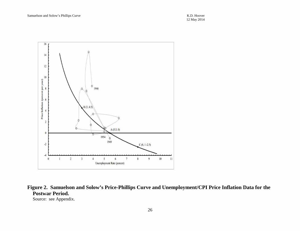
explicitly: point A corresponds to unemployment U = 5½ percent, 0~ =p ; point B corresponds

to U = 3 percent and 5.4~ =p percent per year (p. 192).

Where do these figures come from? Point A corresponds to the translation from wage-

inflation to price-inflation space of Samuelson and Solow’s characterization – noted previously –

of the Postwar period as displaying wage inflation of 2 to 3 percent per year when

unemployment is 5 to 6 percent: θ~~5.25.20~ −=−== wp .

Samuelson and Solow give no explicit account of point B. Translated back into wage-

inflation space, it implies that U = 3 percent, corresponds to θ~~5.25.40.7~ +=+== pw . This

figure is consistent with Samuelson and Solow’s characterization of the wage data at the coarse

level of precision that they adopted throughout their discussion. For example, the regression

lines for the Early 20th Century group lies very nearly parallel and 2¾ points below the

regression line for the Postwar period. As already noted Samuelson and Solow see 3 percent

unemployment as consistent with wage-inflation of 2 to 3 percent per annum in the Early 20th

Century group. The upward shift implied by the regression lines would translate that into U = 3

percent in the Postwar associated with 2.57.25.2~ =+=w percent per annum. That falls short of

the implied value of 0.7~ =w , but then the estimate is based on linear regression curves, and

Samuelson and Solow are clear that hyperbolic curves are appropriate, noting that wage rates rise

the faster, the tighter the labor market. For the same, rightward translation a hyperbolic curve

would imply a higher change in the rate of wage inflation than would a linear curve, presuming

that the reason for the shift in the curve was an increase in the rate of unemployment for any

given rate of wage inflation. Looking directly at the data, note that for the four points in the

Postwar period lying in the interval 2.5 < U < 3.5, the average value of 0.8~ =w , which is higher

than the implied value of 0.7~ =w .


8

Two points are insufficient to determine a hyperbola. Samuelson and Solow do not name

a third point; but, as we already observed, they do associate U = 8.0 with 0~ =w in the Postwar

period. Let us call this point C. Translating into price-inflation space θ~~5.205.2~ −=−=−= wp .

If we assume that Samuelson and Solow fitted a hyperbola to these three points of same form as

the one estimated by Phillips (1958, p. 290), the three points A = (4.5, 0), B = (3.0, 4.5), and C=

(8, –2.5) imply the curve in our Figure 2, corresponding to the equation:

(1) 2155.0~5451.542346.32~ −+−= wp .

Within the limits of measurements readily made with an ordinary ruler, Samuelson and Solow’s

Figure 2 is not just a free-hand curve that passes through the named points A and B, but in fact

corresponds everywhere to hyperbola described in equation (1) and in our Figure 1.

One lesson to be drawn from this exercise is that Samuelson and Solow’s description of

their price-Phillips curve in the legend of their Figure 1 as “roughly estimated” is perfectly apt.

The curve corresponds very precisely to the three points that they single out as salient, but these

points themselves are determined impressionistically. To some extent, their estimation method

echoes that of Phillips. Phillips grouped his data into bins determined by six intervals of the

unemployment rate. He then averaged the data for wage inflation within each bin and assigned

the average value to the median point of the unemployment interval. It is to these six average

data points that he fitted his hyperbola through a procedure that mixed least squares estimation

and an informal adjustment of the intercept term (Phillips 1958, p. 290). This nonstandard

procedure may have been motivated in part by the computational difficulties of implementing

nonlinear regression in the 1950s, but Phillips is also clear that he used the averaging procedure

to abstract from the cyclical properties of the data. Samuelson and Solow’s procedure for

determining the three salient points of their hyperbolic price-Phillips curve amounts to implicit


9

averaging of the same sort. And the relationship of the annual data to the estimated curve is

rather similar to the relationship noted by Phillips. Our Figure 2, shows that the data for the

Postwar period form loops around the hyperbolic Phillips curve, with the beginning of each loop

corresponding to the beginning of business-cycle expansions: the troughs of business cycles

occurring in 1945 4th quarter, 1949, 4th quarter, 1954 2nd quarter, and 1958 2nd quarter. The first

two loops run counterclockwise; while the third runs clockwise. Phillips (1958) had found

counterclockwise loops for U.K. unemployment/wage-inflation data before World War I and

clockwise loops after World War II.

A second lesson to be drawn from our reconstruction of Samuelson and Solow’s

procedure is that their curve is estimated for the postwar period. That fact poses an interpretive

puzzle – one that I will argue trips up Hall and Hart: why if the curve is estimated on postwar

data do Samuelson and Solow refer to it in the legend to their Figure 2 as “roughly estimated

from the last 25 years of American data”? The most likely explanation is based in their view that

the Depression is sui generis. Both the period before the Depression, excepting the years of

World War I and those after World War II are referred to as following a “normal pattern” (p.

189), although the Postwar period is quantitatively distinct, though qualitatively similar, to what

we have called the Early 20th Century group. The Depression period is characterized in their

view by special factors (political or structural) affecting the labor market. Implicitly, Samuelson

and Solow treat it as if it would have been similar to the Postwar period but for those special

factors. And indeed, the key datum, the rate of productivity growth, is 2.80 percent per year for

the period 1933-1957 and nearly identically 2.82 percent per year for 1946-1957.

Samuelson and Solow thus reject the unemployment-wage behavior of the Depression as

informative about the Postwar period, when the special factor were not operative, but are happy


10

to assert the similarity of the two periods in other respects. Their price-Phillips curve is,

therefore, based on the unemployment/wage-inflation relationships of the Postwar period, and a

rough characterization of the productivity data for both the Depression and the Postwar periods.

It is meant to describe roughly what the relationship actually was in the Postwar period and what

it would have been, but for special factors, in the Depression.

Whether or not this explanation is accepted, it would be hard to square Samuelson and

Solow’s actual construction of the price-Phillips curve with reference to the unemployment-wage

behavior of the Depression. They clearly refer to facts that agree with the Postwar data.

Equally, they clearly point out the massive rightward shift of the unemployment/wage-inflation

data in the Depression. Given the way in which the price-Phillips curve is constructed from

translating an implicit wage-Phillips curve by the rate of productivity growth, consistency would

require a similar rightward shift of the price-Phillips curve: the same curve could not represent

both periods, except in the counterfactual sense of representing how they would have been in the

Depression barring special factors.

III. Hall and Hart

Hall and Hart (2012, pp. 65-66) estimate Phillips curves using rates of price inflation based on

both the consumer price index (CPI) and the wholesale price index (WPI) of the form:

(2) tttt UbUbbp ε+++= )/1()/1(~ 2210 ,

where we have adopted our own tilde-notation to indicate rates of growth, the ε indicates a

residual error, and the t subscripts index time. Their estimation period runs 1934-1958, which

takes Samuelson and Solow’s “last twenty-five years of American data” strictly, given their

assumption that Samuelson and Solow’s data ends in 1958. (In the Appendix, I challenge that


11

assumption, but it is not, I believe, consequential for either their results or for my reconstruction

of the price-Phillips curve.) Their estimates yield an unemployment/price-inflation relationship

that is upward-sloping over the range of 0 to 3 percent unemployment when based on the CPI

and over the range 0 to 4 percent unemployment when based on the WPI.

Hall and Hart pose two questions that they believe that their estimates raise:

First, would economic events during the 1960s and 1970s have turned out differently had Samuelson and Solow not weighed in with their Phillips curve? Second, would economic events have turned out differently had Samuelson and Solow presented an empirically estimated Phillips curve like the curves [that Hall and Hart estimate] . . . ? [Hall and Hart 2012, p. 67]

I will return to the first question presently. Meanwhile, consider the presupposition of the

second question – namely, that Hall and Hart’s estimates are ones that Samuelson and Solow

should have made or – at the least – ones that economists in 1960 should have regarded as

informative about the nature of the price-Phillips curve.

Hall and Hart’s presupposition arises from a failure to grasp Samuelson and Solow’s

analysis of the Phillips curve. Hall and Hart’s failure is evident in their wavering between the

view that Samuelson and Solow “estimated the relationship between the rate of inflation and the

unemployment rate” (p. 63, their emphasis) and that they “never estimated their Phillips curve”

(p. 62, abstract, my emphasis).4 Samuelson and Solow did estimate their curve, but they did not

do so by the regression analysis of unemployment/price-inflation data. Rather they did it by

translating points lying on an implicit wage-Phillips curve into unemployment/price-inflation

space. Hall and Hart estimate curves for both CPI and WPI inflation, because in later

4 They also quote Samuelson and Solow’s legend to Figure 2 describing it as “roughly estimated” on p. 69, note 5. The claim that they never estimated the curve is repeated or implied (sometimes multiple times on the same page) on pp. 64, 67, and 68. The Samuelson-Solow price-Phillips curve is also referred to as “hand-drawn” on pp. 62, 64, 67, and 70. It is probably literally true that the curve was hand-drawn; for in 1960 virtually all published graphics would have hand-drawn; but the implication is also that it was drawn free-hand, which given the precision with which Samuelson and Solow’s curve conforms to equation (1) and our Figure 2 is unlikely. As we showed in Section II, Samuelson’s and Solow’s curve is precisely drawn on the basis of a somewhat stylized characterization of the unemployment/wage-inflation data.


12

recollections Solow was unclear about which series they used (p. 64). The internal evidence of

Samuelson and Solow’s paper, however, renders the question moot: Samuelson and Solow’s

method of estimation by translation did not require them to use any price series, since the rates of

price inflation on the curve in their Figure 2 are simply the rates of wage inflation less the

presumed productivity growth rate of 2.5 percent per year. Samuelson and Solow do not refer to

a particular price series (neither to the CPI nor to the WPI) nor to its source, for the simple

reason that they did not use a price series in estimating their curve. They do refer to a particular

wage series, due to Rees (1959) (Samuelson and Solow 1960, p. 187).

The larger problem with Hart and Hall’s approach is that they simply ignore Samuelson

and Solow’s detailed discussion of the wage-unemployment relationship. All they say about it

(buried in an endnote) is that “[t]he backdrop to the Samuelson-Solow Phillips curve, and the

only other diagram in their paper, was a scatter plot of the annual change in wages . . .” (p. 69,

note 6). Samuelson and Solow’s scatterplot may well be the “backdrop” to Samuelson and

Solow’s price-Phillips curve, but the analysis of the data of that scatterplot and the translation of

that analysis into the unemployment/price-inflation space takes place on center stage: it is the

very heart of the matter.

Once this point is understood, it is easy to see that Samuelson and Solow could not have

consistently accepted anything like Hall and Hart’s estimates. Hall and Hart run together three

periods that Samuelson and Solow regard as distinct: the Depression, World War II (included in

our Other group), and the Postwar period. Since Samuelson and Solow go out of their way to

point out that the Depression period behaves like no other, and is both quantitatively and

qualitatively massively different from the Postwar period, the same wage-Phillips curve could

not fit both periods; and, if the same, wage-Phillips curve could not fit both periods, given their


13

method of estimation by translation, ipso facto the same price-Phillips curve could not

characterize both periods. The price-Phillips curve would have to reflect the shift in the

underlying wage-Phillips curve.

The only reason to suppose that Samuelson and Solow could accept Hall and Hart’s

estimates is the statement in the legend to Samuelson and Solow’s Figure 2 that the curve was

“roughly estimated from the last twenty-five years of American data.” I have already offered a

reasonable interpretation of this statement in Section II. Hall and Hart (p. 70) address Samuelson

and Solow’s statement in endnote 16 in which they reject the suggestion of a referee that

Samuelson and Solow’s curve is based on data for the thirteen postwar years corresponding to

the data points “for recent years” that are circled on their unemployment/wage-inflation

scatterplot (Figure 1). They reason, first, that were that so, then the reference in the legend

would be an error; and, more than that, an error that no one in the vast literature on the Phillips

curve had noticed. Of course, the possibility suggested by Section II is that the reference to

twenty-five years is no error at all, but, nonetheless, one should not expect the actual data for the

period from 1934 to 1945 to conform to the Samuelson and Solow’s price-Phillips curve. The

data for that period conforms only counterfactually: had the special circumstances, which

Samuelson and Solow explicitly noted for the Depression and implicitly for World War II, not

occurred, then the data would have conformed. It is the “normal” curve for the whole twenty-

five years, not the actual curve.

It is possible to dig in one’s heels and say, “twenty-five years is twenty-five years; the

data must include the Depression and World War II or Samuelson and Solow must have made an

error – end of story.” But consider the cost of that interpretive move. It implies that Samuelson

and Solow thought that three distinct periods could be treated without any qualification as


14

governed by the same Phillips curve. Yet, they have already rejected the stability of the wage-

Phillips curve relationship across those three periods; and, since their price-Phillips curve is a

simple translation of the wage-Phillips curve by the trend rate of productivity growth, they could

not consistently assert an unstable wage curve and a stable price curve. On the interpretive

principle that we should minimize the attribution of inconsistency, either we should accept my

interpretation that they use twenty-five years of productivity data and offer a counterfactual

interpretation of the relevance of the curve to the earlier periods or, if one were to insist that an

error has been made somewhere, that the error be in the assertion of a twenty-five-year

estimation period – a relative minor mistake – rather than in the assertion of an unstable wage-

Phillips curve, which has the absurd result of making utter nonsense of their discussion of

unemployment and wage change, which is one of the major points of their analysis.

Hall and Hart’s second reason for rejecting the special status of the postwar data in

Samuelson and Solow’s estimates is that they take the referee to imply that the postwar estimates

would not have had the hump-shape of the Phillips curve that they estimated for 1934-1958.

They reëstimated equation (2) for the postwar period and still found a hump-shaped curve. But

this raises the question of Hall and Hart’s functional form. Their equation is quadratic in the

inverse of the unemployment rate (1/U). It is this quadratic form that allows the curve to be

hump shaped. They justify their functional form as the same form used by Lipsey (1960) in his

follow up to Phillips’s study of U.K. wage data. It is, perhaps, more likely than not that

Samuelson and Solow in 1959, when they first drafted their paper, did not know Lipsey’s paper,

which was not published until February 1960; preprints or working papers were not as widely

circulated in those days. We do know, however, that Samuelson and Solow did not have a

quadratic function in mind, but rather a hyperbola, which cannot be hump shaped. To a degree,


15

Hall and Hart’s Phillips curve is hump shaped because of the a priori assumption of a quadratic

form. Of course, we cannot say that the hyperbolic curve is automatically to be preferred to a

quadratic curve, but simply finding the built-in hump shape within the range of positive

unemployment rates does not, in itself, show the inferiority of the hyperbolic curve. And the

acceptability of the hyperbolic curve cannot be tested within the framework of the quadratic

curve, since it is not a special case of it.

We can, I believe, conclude that Samuelson and Solow would have rejected – indeed,

should have rejected – Hall and Hart’s estimates. Samuelson and Solow were fully aware that

the data clearly came from different regimes and could not be sensibly characterized by a single,

stable bivariate curve. They would never have presented such estimates, so that Hall and Hart’s

second “what if” never gets off the ground. Yet, suppose that they had, what can we say about

Hall and Hart’s first question: “would economic events during the 1960s and 1970s have turned

out differently had Samuelson and Solow not weighed in with their Phillips curve?” Again,

consider the presupposition of the question. Hall and Hart suppose that Samuelson and Solow’s

Phillips curve was directly and deeply influential with respect to economic policy in the 1960s

and 1970s. This is, I believe, largely a myth (see Forder 2010a).

Hall and Hart’s main support for the claim comes from two sources: a quotation from the

Council of Economic Advisers in the Economic Report of the President (Kennedy 1962, p. 46;

cited by Hall and Hart 2012, p. 64) that says that policy should aim to reduce unemployment

without creating demand-induced inflation, and references to three papers by Robert Leeson

(1997a, 1997b, and 1997c). The statement of the President’s Council was in 1962 by no means

novel nor did it in any way require Samuelson and Solow’s price-Phillips curve (or any other

Phillips curve) for support. The idea that demand hitting a high level both reduced


16

unemployment and risked higher inflation was an old one. It is found in Keynes’s General

Theory (1936), it formed the basis for discussions and quantifications of the “inflationary gap,”

which had been widespread in the 1940s and 1950s, and it was ubiquitous in the literature to

which Samuelson and Solow directed the first half of their paper – before their discussion of the

Phillips curve – to clarifying. Phillips (1958, esp. pp. 298-299), like Samuelson and Solow, was

concerned to distinguish empirically between cost-push and demand-pull inflation, and, of

course, the inverse relationship of aggregate demand and unemployment was widely accepted.

It would be easy to multiply examples of these ideas before Phillips or Samuelson and

Solow’s papers, but one example will do:

Many of us know about the thesis of The Economist of London on the ‘uneasy triangle’–stable prices, full employment and strong economic pressure by organized labor, industry and agriculture” (Bronfenbrenner 1957, pp. 20-21).5

The report of the President’s Council cited by Hall and Hart nowhere mentions the

Phillips curve. It nowhere mentions the idea of a stable tradeoff between inflation and

unemployment resulting in a menu for policy. Rather it points to the well-known situation of

high levels of demand being both good for employment and bad for inflation – and it, tries to put

a number on the sweet spot for unemployment. I do not mean to suggest that policy was not

influenced by Samuelson and Solow’s analysis. That seems unlikely, given that Solow was a

staff member of, and Samuelson a consultant to, the Council of Economic Advisers in 1962

(Kennedy 1962, p. 196). Surely, Samuelson and Solow drew on the range of their economic

insights in fulfilling their public duties. Instead, I am merely suggesting that the actual policies

advocated, not only in 1962, but throughout the 1960s would hardly have been different, with or

without Samuelson and Solow’s price-Phillips curve (or, indeed, with or without Phillips’s wage-

5 Even something like the Phillips curve itself might well have predated Phillips, see Fisher (1926), Humphrey (1985, 1986).


17

curve), as long as they were formulated by American Keynesians of the stripe of Samuelson,

Solow, James Tobin, Walter Heller, and Kermit Gordon – the last three being the actual

members of the Council in 1962.

Hall and Hart’s also cite Leeson’s papers in support of their thesis that the Samuelson and

Solow’s price-Phillips curve was critical for policymakers. But examination of those papers

does not reveal any evidence that is more compelling than the thin reed of the 1962 report of the

Council of Economic Advisers.

The idea of the Phillips curve as dominating economic policy in the 1960s, appears to be

largely a bit of Whig history, whose best-known proponent was Milton Friedman in his

presidential address to the American Economic Association in 1967 (Friedman 1968). Before

Friedman’s address and before the Phelps’s (1967) invention of the expectations-augmented

Phillips curve, the Phillips curve received a moderate amount of academic attention. A search of

economics articles in JSTOR for the term “Phillips curve” between 1958 and 1967 yields 44

articles using the term. A search of the period after Friedman’s address, 1968 to the present

yields 4,315 articles.6 The role of Friedman in the invention of the Phillips curve as a vastly

influential policy tool has been discussed in great detail by James Forder (2010b; forthcoming).

There is little doubt that Samuelson and Solow saw the price-Phillips curve as a

relationship that might be relevant to policy. The legend to their Figure 2 refers to a “menu.”

Hall and Hart (2012, p. 63, citing Leeson 1997b) interpret a later interview with Samuelson and

Solow in which they refer to the Phillips curve as “reversible” as “downplay[ing] the possibility

of an unstable Phillips curve.” Samuelson and Solow (1960, p. 189) had already discussed

reversibility in their article, by which they seem to mean whether a relationship is stable enough

that policy might move the economy along the menu without shifting it too much or destroying 6 The search covered economics articles only and was conducted on 14 May 2014.


18

it. This discussion appears in the midst of the discussion of the instability of the

unemployment/wage-inflation relationship that Hall and Hart essentially ignore. In fact,

Samuelson and Solow are modest. With respect to the quantification of the price-Phillips curve,

they caution “these are simply our best guesses,” and they immediately point out that their curve

may provide a reversible menu only in the short run:

All of our discussion has been phrased in short-run terms, dealing with what might happen in the next few years. It would be wrong, though, to think that our Figure 2 menu that relates obtainable price and unemployment behavior will maintain its same shape in the longer run. What we do in a policy way during the next few years might cause [the price-Phillips curve] to shift in a definite way. [Samuelson and Solow 1960, p. 193]

One mechanism that they consider anticipates Phelps and Friedman:

after they had produced a low-pressure economy, the believers in demand-pull might be disappointed in the short run; i.e., prices might continue to rise even though unemployment was considerable. Nevertheless, it might be that the low-pressure demand would so act upon wage and other expectations as to shift the curve downward in the longer run— so that over a decade, the economy might enjoy higher employment with price stability than our present-day estimate would indicate. [p. 193]

And they say that the biggest question not addressed in their article is whether institutional or

policy arrangements can shift the Phillips curve downward to the left. Far from downplaying the

possibility of an unstable curve, Samuelson and Solow indicate that policies that shift the curve

to a more favorable tradeoff might be particularly desirable.

IV. A Want of Intellectual Charity

The best history and the best criticism require a charitable reading of the subjects under study. It

is essential to see exactly what they were trying to do and to attribute to them reasonable and

defensible choices wherever that is possible. One should make the best case for the subjects

under study, and in that way one can sometimes make a much stronger case for where they really

went wrong and sometimes, against initial expectation, see that they did not go wrong after all.


19

In offering estimates that combine the data of the 1930s and early 1940s with postwar data,

attributing a stability to the data that was never claimed and, indeed warned against; in

employing a functional form that cannot possibly have the properties of the hyperbola; in

ignoring the central discussion of unemployment and wage-inflation; in failing to try to

understand how that discussion is related to the construction of the price-Phillips curve; in

treating “estimated” as if it could mean only estimated by a regression of price inflation on

unemployment; and in assuming that the specification of the period of twenty-five years was

open to only one reasonable interpretation, Hall and Hart have not only failed to give Samuelson

and Solow a charitable reading, but have absurdly attributed a notion of a stable Phillips curve

over a period for which Samuelson and Solow explicitly deny that such a stable curve exists.

The price paid is simply that they have failed to understand either Samuelson and Solow’s point

or its historical importance. Samuelson and Solow’s article is a tour d’force of back-of-the-

envelope economics. It was an exploration, not a destination; an invitation to further research,

not a report of a careful study; a suggestion of a possibility for policy guidance, not a blueprint

for actual policymakers. Their conclusions were put modestly. The history of the exploration of

the Phillips curve in the 1960s and, especially, after the popularization of the expectations-

augmented Phillips curve in the wake of Friedman’s presidential address demonstrated that the

potential of Samuelson and Solow’s article as a catalyst for important research was largely

realized.

Appendix. The Data

Only two data series are actually deployed explicitly in Samuelson and Solow’s paper: “average

hourly earnings in manufacturing, including supplements,” which they refer to as Rees’s data (p.


20

187) and the unemployment rate. Rees (1959, Table 1, pp. 15-16) presents this data, as well as

data for labor productivity (with a gap got productivity for the years 1890-1898) for the period

1889-1957. Samuelson and Solow do not specify a source for the unemployment data, but Hall

and Hart (2012, p. 64) say that Solow recollects that Lebergott’s unemployment series was

spliced to the series from the Bureau of Labor Statistics. The data in Lebergott (1957) run 1900-

1954.

Hall and Hart, as we have noted, ignore the wage data, and they say that they take the

price and unemployment data that they use from the Economic Report of the President

(Eisenhower 1959), noting that it was available to Samuelson and Solow. They assume that,

because 1958 was the last full year before Samuelson and Solow wrote their paper, only data up

to 1958 would have been used in their study. This is, I believe, an incorrect conclusion. It is true

that Samuelson and Solow wrote their paper for presentation on 28 December 1959. It was,

however, not published until May 1960. The Economic Report of the President (Eisenhower

1960), in fact contains unemployment data through 1959, and was published on 20 January 1960.

They would, therefore, have had an opportunity to update the data through 1959 when revising

the paper for publication.

There is a stronger reason to believe that Samuelson and Solow did use data through

1959. Their Figure 1 circles thirteen data points, which it says are from “recent years.” Mapping

those points onto the actual data shows that they do not include 1945 or 1946, but do have points

that correspond to all the dates from the eleven years 1947-1957. The additional two points

appear to correspond to 1958 and 1959 once a choice has been made for unemployment rates for

those years.


21

The problem of choice of unemployment rates arises because the Economic Report of the

President presents an series on old and a new definitions for unemployment rates. The old series

agrees with the Lebergott series. What is more, Samuelson and Solow say that the

unemployment rate for 1953 is 2.5 percent, which is the value for the old series – the value for

the new series is 2.9 percent. They also say that the value for 1958 is 6.2 percent. But where did

they get that number? The old series stops in 1957 and the value for the new series is 6.8

percent. My guess is that they either obtained a compatible number to the old series from

Lebergott or some other researcher directly or that they interpolated the old series value from its

relationship to the new series, which starts in 1947. My own interpolation using a regression of

the old series on the new series yields a value of 6.3 for unemployment in 1958. Hall and Hart

use the data from the old series until 1946 and, incorrectly, data from the new series from 1947-

1958.7

A question arises as to which years are reflected in Samuelson and Solow’s Figure 1.

Hall and Hart (2012, p. 70, note 16) say that it reflects 50 or 60 years. But a careful count of the

points on the scatterplot show that they number 67. If the data end in 1959, then the period

covered would be 1893-1959. This span does not have the virtue of starting as early as the Rees

data (1890, allowing for the loss of one year to calculate growth rates) or for starting as late as

1900, dictated by the coverage of the Lebergott data. One possibility is that they really did start

in 1893. Another possibility is that they omitted two data points by mistake – something easily

done on a graph obviously constructed by hand. A third possibility would be that two of the

points were so close to two other points that they failed to show distinctly. Something like this

happens on our Figure 1 in which the points for 1955 and 1957 are so close that the circles are

not distinct and what are actually fourteen circled points (1946-1959) appear to be thirteen. It is 7 A fact determined by comparing data that sent to be privately for the series that they call ublsnew.


22

conceivable that careful measurement of the positions of the points on Samuelson and Solow’s

Figure 1 might allow us to definitely say which dates are represented there, but it hardly seems

an exercise that would repay the trouble. None of the issues raised in this or Hall and Hart’s

paper would be resolved on that basis.

The actual data used in this paper can be downloaded from:

public.econ.duke.edu/~kdh9/Source%20Materials/Software%20and%20Data/DataandDocumentation_for_SandS_

Paper.xlsx

The data run 1890 to 1959 with wage and productivity data converted to growth rates, and the

basic data is defined as follows:

Labor Productivity Output per Man-hour, Manufacturing Units : index 1929=100; Source: 1889-1957 (with lacunae 1890-1898): Rees (1959), column 6.

Prices

Consumer Price Index Units: index 1957=100; Source: 1889-1957: Rees (1959), column 4;

1958-1959: Eisenhower (1960), Table D-38 (index 1947-1949 = 100 converted to 1957=100).

Wage Rate

Total Compensation (including Wage Supplements) Units: dollars per hour; Source: 1889-1957: Rees (1959, Table 1, column 3);

1958-1959: Eisenhower (1960), Table D-24 adjusted as follows: Compensation_Rees = 1.1584Compensation_Eisenhower + 0.0283

Unemployment Rate

Civilian Labor Force Unemployed as a Percentage of the Civilian Labor Force Units: percent; Source: 1890-1899: Sutch and Carter (2014), Table Ba470;

1900-1928 Department of Commerce (1960), Series D47; 1929-1957: Eisenhower (1960), Table D17, old definitions; 1958-1959: Eisenhower (1960), Table D17, new definitions, adjusted as follows:

Unemployment_old = 0.9712Unemployment_new – 0.2597 (Note: these series are agree with, or are based on the methods of, Lebergott 1957.)


23

References

Bronfenbrenner, Martin. (1957) “Secular Inflation and Shibboleths,” Challenge 6(3), 17-22.

Department of Commerce, U.S. (1960) Historical statistics of the United States, colonial times to 1957; a Statistical abstract supplement. Washington: Government Printing Office, 1960.

Eisenhower, Dwight D. (1959) Economic Report of the President. Washington, D.C.: United States Government Printing Office.

Eisenhower, Dwight D. (1960) Economic Report of the President. Washington, D.C.: United States Government Printing Office.

Fisher, Irving. (1926) “A Statistical Relation between Unemployment and Price Changes,” International Labour Review, 13(6), 785–92. Reprinted “I Discovered the Phillips Curve: A Statistical Relation between Unemployment and Price Changes," Journal of Political Economy, 81(2, Part 1), pp. 496–502.

Forder, James. (2010a) “Economists on Samuelson and Solow on the Phillips Curve,” University of Oxford, Department of Economics, Economics Series Working Papers: 516.

Forder, James. (2010b) “Friedman's Nobel Lecture and the Phillips Curve Myth,” Journal of the History of Economic Thought 32(3), 329-348.

Forder, James (forthcoming) Macroeconomics and the Phillips Curve Myth. Oxford: Oxford University Press.

Friedman, Milton. (1968) “The Role of Monetary Policy,” American Economic Review 58(1), 1-17.

Hall, Thomas E. and William R. Hart. (2012) “The Samuelson-Solow Phillips Curve and the Great Inflation,” History of Economics Review 55(1), 62-72.

Humphrey, Thomas M. (1985) “ The Early History of the Phillips Curve,” Federal Reserve Bank of Richmond Economic Review 71(5), 17-24.

Humphrey, Thomas M. (1986) “Of Hume, Thornton, the Quantity Theory, and the Phillips Curve,” in Essays on Inflation, 5th ed. Richmond: Federal Reserve Bank of Richmond pp. 128-33.

Kennedy, John F. (1962) Economic Report of the President. Washington, D.C.: United States Government Printing Office.

Keynes, John Maynard. (1936) The General Theory of Employment, Interest, and Money. London: Macmillan.

Leeson, Robert. (1997a) “The Tradeoff Interpretation of Phillips’ Dynamic Stabilization Exercise,” Economica N.S. 64(253), 155-171.

Leeson, Robert. (1997b) “The Political Economy of the Inflation-Unemployment Tradeoff,” History of Political Economy 29(1), 117-156.

Leeson, Robert. (1997c) “The Eclipse of the Goal of Zero Inflation,” History of Political Economy 29(3), 445-496.


24

Phelps, Edmund S. “Phillips Curves, Expectations of Inflation and Optimal Unemployment over Time,’ Economica N.S. 34(135), 254-281.

Phillips. A. W. H. (1958) “The Relation between Unemployment and the Rate of Change of Money Wage Rates in the United Kingdom, 1861-1957,” Economica, N.S. 25(100), 283-299.

Rees, Albert (1959) “Patterns of wages, prices, and productivity,” in The American Assembly, Columbia University, Wages, Prices, Profits and Productivity: Background Papers and Final Report of the Fifteenth American Assembly, Arden House, Harriman Campus of Columbia University, Harriman, New York April 30-May 3, 1959. Harriman, New York: The American Assembly, Columbia University, 1959, ch. 1, pp. 11-35.

Samuelson, Paul A. and Robert M. Solow. (1960) “Analytical Aspects of Anti-Inflation Policy,” American Economic Review 50(2), 177-194.

Sutch, Richard and Susan B. Carter, editors. (2014) Historical Statistics of the United States. Millennial Edition Online . Cambridge University Press; downloaded 4/30/14.

25

Figure 1. Unemployment and Wage Inflation 1890-1959.

Data and regression lines for four periods: Early 20th Century (1901-1914; 1919-1929); Depression (1933-1941); Postwar (1946-1959); Other (1890-1900; 1915-1918; 1930-1932) Source: see Appendix.


26

Figure 2. Samuelson and Solow’s Price-Phillips Curve and Unemployment/CPI Price Inflation Data for the

Postwar Period. Source: see Appendix.

The Genesis of Samuelson and Solow’s Price-Inflation ...public.econ.duke.edu/~kdh9/Source...

Documents

Transcript of The Genesis of Samuelson and Solow’s Price-Inflation ...public.econ.duke.edu/~kdh9/Source...