The Gender Gap in Price Negotiations:Evidence from New Car Sales∗

Ambarish Chandra Sumeet Gulati James Sallee

December 6, 2013

Abstract

Increases in the educational attainment and labor force participation of women haveconstituted some of the biggest societal changes in North America over the past fewdecades. Yet, economic research into the consequences of this phenomenon has beenrestricted almost exclusively to the labor market. We investigate whether women’sperformance in price negotiations has improved relative to that of men. Using detailedtransaction level data from the automobile industry, we show that the age premiumrises more steeply for women than for men, consistent with the hypothesis that higherlevels of education and work experience have led women to close the gender gap in thisindustry.

Keywords: Gender; Age; Automobiles; Negotiations; Bargaining. JEL Codes: J14,J16, L62.

∗Chandra: Department of Economics, University at Albany, ambarishchandra@gmail.com; Gulati: Foodand Resource Economics, University of British Columbia, sgulati@mail.ubc.ca; Sallee: Harris School ofPublic Policy, University of Chicago, sallee@uchicago.edu

1

1 Introduction

The last several decades have seen dramatic changes in the educational attainment andlabor force participation of women. In North America, women now make up about 45% ofthe labor force, and almost 60% of college graduates, a stark change from the 1970s. Thisphenomenon has had huge societal effects, such as on the rate and age of marriage, as wellas on fertility rates. It has had equally profound economic impacts, such as on wages andcareer opportunities for women.

Most prior economic research into the consequences of increased women’s education andemployment has focused on the labor market itself. Economists have documented the effectson women’s wages, most notably the fact that the gender wage gap has narrowed but notclosed.1 Various studies have also examined changes in female representation in managerialpositions.2 There has, however, been remarkably little research on the impact of thesesocietal changes in other markets. In particular, few prior studies have examined whetherthere have been changes in the prices that women pay in important transactions that involvenegotiations, other than studies of wage negotiations.3

Personal interaction and negotiation influence the prices or quality of products in severalkey markets. We negotiate with service providers, financial institutions and, most impor-tantly, in the markets for housing and automobiles. Individual characteristics can potentiallyplay an important role in negotiated outcomes. In this paper, we examine whether pricesnegotiated by women have shown significant improvements over time. In particular, we askwhether older women today, who on average have lower education levels and had a lowerlikelihood of having been employed when in their 20s and 30s, fare worse in price negotiationsthan younger women. We examine how each cohort of women performs relative to men oftheir same age, treating these men as a control group since they did not undergo the sametransformative experiences that women did.

It is challenging to identify appropriate markets for this study. The ideal market wouldprovide data on both negotiated prices and consumer demographics, and would also involvetransactions of identical goods, or else enough data on varying characteristics to controlfor systematic differences in the choice of goods by different types of consumers. However,prices are generally not open to negotiation in many everyday markets where the personalcharacteristics of consumers are observed. Conversely, it is difficult to obtain price datain markets with negotiated prices since these usually occur in private or informal settings;for example, when bargaining for loans with financial institutions, selling goods such asused cars via Craigslist, or hiring contractors to perform residential services. The housingmarket appears promising, but it is rare to find housing transactions that involve identicalunits — a sample of housing transactions will always involve considerable heterogeneity incharacteristics that are difficult to control for precisely.

Therefore, we look to the new car market, which we believe offers the ideal setting for ourstudy for a number of reasons. First, final prices in this market are commonly negotiated

1See, for example, Blau and Kahn (2007) and O’Neill (2003).2See Bertrand and Hallock (2001) and Bertrand et al. (2010).3Specifically, we are not aware of prior studies of this issue in the Economics literature. Other fields, par-

ticularly Psychology, have investigated this topic, though primarily in laboratory settings. See Stuhlmacherand Walters (1999) for a survey.

2

and there can be differences of hundreds of dollars in the amounts that different consumerspay for the same new car. Second, this market involves the sale of many identical goods:knowing the make, model and trim of a vehicle pins down almost exactly the type of goodthat different consumers buy. Other differences in transactions, such as the location of cardealers and the timing of the transaction, can easily be controlled for. Finally, we have dataon two key elements of new car transactions: the final price paid by consumers, and thedealer’s invoice price, which represents the opportunity cost to the dealer of selling the car,and therefore includes the cost of unobserved options purchased by consumers. Thereforewe can construct precise measures of the dealer’s profit margin — which is rare in almostany industry — and examine whether these margins are systematically different for differenttypes of consumers.

Previous research into the automobile industry has, of course, examined the role of genderand other demographics in price negotiations. Famously, Ayres and Siegelman (1995) usedan audit study and found that women and minorities are disadvantaged in the new carmarket, as both groups are offered higher initial prices by dealers as well as negotiate higherfinal prices. Since then, a number of studies have re-examined the issue of gender differencesin the new car market, including Goldberg (1996) and Harless and Hoffer (2002). Both thosestudies cast doubt on the finding that women pay more for new cars. More recently, Mortonet al. (2003) show that, while minority customers pay a higher price than others, this can beexplained by their lower access to search and referral services. Similarly, Busse et al. (2013)find that women are quoted higher vehicle repair prices than men when callers signal thatthey are uninformed about prices, but these differences disappear when callers mention anexpected price for the repair.

Importantly, no previous study has examined the interaction of age and gender in thenew car market, especially in the context of possibly different behavior exhibited by differentcohorts.4 Our study does so explicitly, and also makes other contributions to the existingliterature. First, we use a dataset involving more than half a million transactions in the newcar market, a far larger sample than was available in the earlier studies described above.Second, we have data on both final transaction prices and dealers’ invoice prices, whichallows us to calculate and study dealer margins. Third, the large sample allows us to divideconsumers into fine age and gender categories, and also to use a large set of fixed-effects thatcontrol precisely for vehicle characteristics.5

Following Busse et al. (2013), we estimate equations for transaction prices and dealermargins controlling for a range of demand and supply covariates. Our data come from JDPower, and are drawn from a very large set of new car transactions in Canada between2004 and 2009. Benefiting from the large size of our sample, we identify variations in dealermargins within model, year, province and trim variations, and across several gender andage categories. Our estimating strategy minimizes the potential impact of other influences:whether the vehicle was leased or financed; whether it was purchased at the end of the month

4Harless and Hoffer (2002) do examine customer age, finding that older consumers generally pay moreon average, but do not examine the relative performance of each gender across age cohorts. Langer (2011)examines the interaction between the gender and marital status of consumers, but does not focus on cohorteffects either.

5This also allows us to use simple methods with confidence, as we know both the trim level and the costof the vehicle, in contrast to, say, Langer (2011).

3

or year, when dealers face incentives to increase sales; whether certain dealers were morelikely to offer discounts in a manner correlated with customer demographics; whether thevehicle was in greater demand — measured by the average time the particular model stayedon dealers lots — and whether there was a trade-in vehicle associated with the transaction.

We uncover an important interaction between age and gender in the market for new cars.First, we find that dealer margins rise among older customers, even after controlling forall observable aspects of the transaction. Second, we find that the age premium rises moresteeply for women than for men. As a result, young women pay the least for new cars whereasolder women pay the most. The under- and over-payments by these groups of women arenot only significantly different from zero and from each other, but also significantly differentthan the premiums paid by men of the same age. Thus, even if there exist secular age effectsthat may explain our results to some extent, the differences in outcomes between youngerand older women are even more pronounced and require further explanation.

We believe that our results are consistent with the education and labor market disparitiesbetween women of different age cohorts. Women above the age of 65, who generate thehighest dealer margins, are less likely to have participated in the labor force when they wereyounger, or to have obtained a college degree, than women under 25, who generate the lowestmargins. These differences can potentially cause older women to have lower information inthe new car market and possibly also to negotiate with less confidence. The price differencesthat we observe may be exacerbated by demographic trends. Beyond the age of 65, womenstart to rapidly outnumber men in the population, due to lower survival rates for the latter.Thus, a large number of women in this cohort are single, either because of the death ofa spouse or because of divorce. Many of these women may have relied on their spousesto purchase new cars in the past — we see evidence that this is true even today, by theconsiderably lower rates of women purchasing cars among the age group most likely to bemarried. Thus, older women who buy new cars may be doing so for the first time, in contrastto men of the same age.

We also consider alternative explanations for our results, in particular the possibilitythat the higher age premium for women may be an ongoing phenomenon. The evidencesupports our hypothesis that it is in fact driven by labor market and education changes, butwe acknowledge that our results do not conclusively prove this. Doing so would require atime series of vehicle transactions involving consumers of different ages; essentially multiplerepetitions of our data over a very long period of time. But such data do not exist inthe new car market — since large samples of vehicle sales have become available only inrecent years — and certainly do not exist in other markets, due to the difficulties describedabove. Nevertheless, ours is the first study to examine this issue and to provide evidencethat the gender disparities may be caused by women’s education and labor market changes.Moreover, our results are cleanly identified and extremely robust. Confirmation of this resultwill require it to be repeated in future studies.

In Section 2 we present the data used in our study. In Section 3 we present the empiricalframework. Section 4 contains our main results along with various checks for the robustnessof our findings. Section 5 discusses various explanations for our results. We provide a briefconclusion in Section 6.

4

2 Data

Our analysis uses data provided by automobile dealers to a major market research firm.This data includes more than 250 key observations for each vehicle transaction including:a) vehicle characteristics: vehicle trim, number of doors, engine type, transmission etc;b) transaction characteristics: suggested retail price, transacted price, cost of the vehicleincluding factory and dealer installed accessories, whether the vehicle was financed, leasedor a cash purchase, rebates offered, and how long the vehicle was on the dealers lot; c) trade-incharacteristics: the price of the trade-in vehicle, and its under or over valuation; d) customerdemographics: gender, age, province of residence, and province of purchase. The selection ofdealers is not random, as dealers must agree to be included in the database. However, it isthe most comprehensive dataset on vehicle purchase transactions. Our sample of the data isapproximately 20% of new vehicle sales in Canada from May 1st, 2004 to April 15th, 2009,a total of 1,137,573 transactions.

The automobile industry in Canada is very similar to its US counterpart. The two mar-kets are in fact extremely integrated, and the set of manufacturers and models is almostexactly the same, as is the process of customer negotiation for new cars with dealers. Cana-dian prices tend to be somewhat higher than in the US, but in most other respects the twoindustries are indistinguishable. We have no reason to believe that our findings are uniqueto the Canadian autombile industry.

2.1 Sample Selection

We comparing our sample of transactions data with aggregate sales data provided by DesrosiersAutomotive Consultants, and population data from Statistics Canada in order to determinehow representative our sample is. Consider the distribution of transactions by major man-ufacturer (Table 1). The first two columns in Table 1 are the number of transactions andpercentage of overall transactions for the year 2006 from our sample of the PIN data. Thethird column is the percentage of sales by manufacturer from data compiled by DesrosiersAutomotive Consultants for the same year—2006, capturing all sales in Canada. Our sam-ple appears to over-represent sales by GM, Toyota, Nissan, and VW. Similarly, our sampleunder-represents Chrysler, Ford, Honda, and other manufacturers. THe differences are,however, not large.

Next, we illustrate the distribution of vehicle transactions across provinces for the year2006 (see Table 2). The first two columns are the number of transactions and percentageof total transactions for the PIN data. The third column is the sales share calculated fromdata provided by Desrosiers, and the fourth column has the percentage of population foreach province estimated by Statistics Canada.6 Our sample clearly over-represents Alberta,and to a certain extent Quebec, at the expense of slight under-representation of the otherprovinces.

These tables most likely illustrate dealer sample selection issues. For this reason, we arecareful not to draw conclusions across provinces and manufacturers. Our estimating strategy(discussed later) focuses on effects within provinces and car models. Thus, sample selection

6Source: Statistics Canada, Canadian Socioeconomic Database, table 051-0001.

5

Manufacturer No. Column%

AggregateSales %

GM 53458 28.1 26.0Toyota 31859 16.8 12.2Chryl 22703 11.9 13.7Ford 20934 11.0 14.2Honda 18732 9.9 10.3Nissan 9603 5.1 4.1Korea 7232 3.8 6.2Mazda 9001 4.7 5.0VW 6689 3.5 2.7Japan 5083 2.7 2.4Europe 2633 1.4 1.9BMW 2174 1.1 1.2Total 190101 100.0 100.0

Source: Authors Calculations-JD Power PIN, and Desrosiers Data

Table 1: Sales Across Manufacturers (2006).

Province No. Column%

Sale-share

%

Pop-share

%

Ontario (ON) 65453 34.4 37.5 38.9Quebec (QC) 51728 27.2 24.7 23.4Alberta (AB) 42660 22.4 14.9 10.5British Columbia (BC) 19156 10.1 11.7 13.0Newfoundland and Labrador (NL) 2501 1.3 1.5 1.6Manitoba (MB) 3310 1.7 2.7 3.6Nova Scotia (NS) 1904 1.0 2.9 2.9Saskatchewan (SK) 2040 1.1 2.4 3.0NorthWest Territories (NT) 710 0.4 NA 0.1New Brunswick (NB) 487 0.3 2.1 2.3Yukon (YT) 152 0.1 NA 0.1Total 190101 100.0 100.0 100.0

Source: Authors Calculations, PIN and Desrosiers Data, STATCAN CANSIM Table 051-0001.

Table 2: Sales Across Provinces (2006).

6

Segment Mean Median

MaleCust

FemaleCust

CustPrice

DealerMarg

TurnDays

CustAge

CustPrice

DealerMarg

TurnDays

CustAge

Compact (37%) 46.7% 53.3% $19,936 $1,314 44.8 44.5 $19,529 $1,238 14 44Full (0%) 75.8% 24.2% $35,285 $1,204 55.3 67.8 $35,215 $1,224 8 70Luxury (4%) 68.9% 31.1% $47,712 $2,701 53.4 50.4 $44,968 $2,550 19 50Midsize (13%) 62.0% 38.0% $28,617 $1,647 58.9 51.3 $27,871 $1,555 20 51Pickup (13%) 83.0% 17.0% $39,315 $2,209 61.0 43.4 $38,604 $1,865 26 43SUV (20%) 59.9% 40.1% $35,555 $1,943 49.8 45.6 $32,219 $1,702 16 45Sports (1%) 67.6% 32.4% $42,690 $3,075 58.9 43.1 $35,041 $2,240 18 44Van (9%) 67.1% 32.9% $28,423 $1,346 71.3 47.8 $27,800 $1,361 36 45Total (100%) 59.6% 40.4% $29,255 $1,705 53.0 46.0 $26,373 $1,463 18 46

Source: Authors Calculations

Table 3: Statistics across Segments.

should not be a concern for the implications of our results.In Table 3 we present selected summary statistics across vehicle segments. The bottom

row presents summary statistics for the entire dataset. The median vehicle sold for approx-imately $26,373, generated $1463 in margin for the dealer, was on her lot for 18 days, andwas bought by a 46 year old male customer. Full size (with relatively few data-points) andluxury vehicles are purchased by older individuals. Luxury vehicles have the highest values.Compact and full size vehicles are sold in fewer days than other segments.

In the next few tables we highlight the role played by gender and age in the automobilemarket. In our data, gender is determined by matching the entered name with expectedgender. There are several observations where gender or age cannot be determined, andwe drop these. We also drop observations with very small and very large dealer margins; inparticular the bottom and top 1% of the data. These correspond to unusual models, typicallywith very high purchase prices, which can potentially skew the results.7 This leaves us withabout 510,000 observations (from over a million earlier). All summary statistics presentedin this data description, as well as our later regressions, are from this smaller subset.

Approximately, 59% of all transactions have male customers (see Table 4). We divide ageinto 11 categories of 5-year intervals. Approximately 24% of our transactions have customersunder the age of 35. Women outnumber men in the under 25 age category, but not in anyother category. We observe an interesting ‘missing women’ pattern. Women comprise 46%of transactions among the under 35 year-olds. This shrinks to 41% in midage category, andfurther to 36% in the category aged above 55. With little other information, it is difficult tohypothesize an explanation.

In Figure 1 we illustrate how the mean transacted price, and vehicle cost varies withage in our data. Both mean price and cost peak for customers aged 39 years, at $30,306,and $28,900 respectively. Both younger and older customers around this age buy cheaper

7This procedure drops transactions where the dealer margin was greater than $7300, or where the dealerlost more than $2200 on the sale.

7

Gender

Age Category Male Female TotalNo. Col

%Row

%No. Col

%Row

%No. Col

%Row

%

Age Under 25 15301 5.1 47.8 16716 7.9 52.2 32017 6.3 100.0Age 25-30 22801 7.6 52.3 20776 9.8 47.7 43577 8.5 100.0Age 30-35 28251 9.5 58.0 20493 9.6 42.0 48744 9.5 100.0Age 35-40 31889 10.7 60.0 21270 10.0 40.0 53159 10.4 100.0Age 40-45 36553 12.2 58.1 26379 12.4 41.9 62932 12.3 100.0Age 45-50 38623 12.9 57.4 28631 13.5 42.6 67254 13.2 100.0Age 50-55 35561 11.9 58.0 25789 12.1 42.0 61350 12.0 100.0Age 55-60 29708 10.0 59.8 19976 9.4 40.2 49684 9.7 100.0Age 60-65 21921 7.3 62.4 13231 6.2 37.6 35152 6.9 100.0Age 65-70 15341 5.1 64.3 8531 4.0 35.7 23872 4.7 100.0Age Over 70 22554 7.6 68.1 10571 5.0 31.9 33125 6.5 100.0Total 298503 100.0 58.4 212363 100.0 41.6 510866 100.0 100.0

Source: Authors Calculations

Table 4: Sales by Age Category

vehicles on average.A similar trend in dealer margin is illustrated in Figure 2. Like the average price and

cost, dealer margin rises with age and then declines after a peak of $1769 at age 50. Thisdistribution is marked by a relatively flat section from age 33 (average dealer margin $1707)to age 59 (average dealer margin $1707) with sharper drop offs on either side.

Overall, men purchase more expensive vehicles, with an average price of $31,075 versus$26,589 for females (see Table 5). Male customers also generate higher margins for their deal-ers at $1,784 versus $1,590 generated by female customers. This difference carries throughwithin vehicle segments as well.

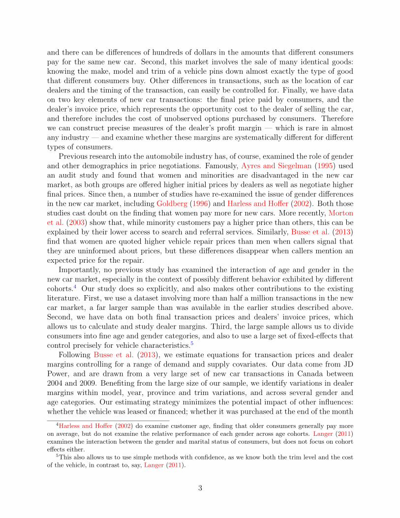
We can also illustrate how vehicle prices and cost vary across age by gender. In Figure 3we illustrate how the mean transacted price, and vehicle cost varies with age across gender.Male customers aged 42 years, buy the most expensive vehicles at $31,709, and femalecustomers aged 39 years buy their most expensive vehicles at $26,781. Both younger andolder customers around this age buy cheaper vehicles on average.

3 Estimating Strategy

Consider a simple linear model explaining dealer profits from a particular vehicle transaction.Define xm as model characteristics, xd as dealer characteristics, and zg as a group identifier∀g ∈ 1, 2 (for simplicity we assume only two groups). Dealer d’s profits from selling modelm to customer i from group g are:

πmidg = xmβ + xdγ + zgδ + εi, (1)

8

Figure 1: Price and Vehicle Cost by Age

2200

024

000

2600

028

000

3000

0Pr

ice

& Ve

hicl

e C

ost (

$)

20 40 60 80Age

Mean Vehicle Price Mean Vehicle Cost

where β, γ, δ are the associated coefficients, and εi is the error term. We identify a marketdisparity across groups if δ 6= 0.

3.1 Omitted Variable and Misspecification Bias in Estimating Dis-crimination.

Equation 1 above helps us identify a market disparity, it does not help us identify ‘discrim-ination.’ Consider a special case for the two groups, where the true value of δ = 0 andβ1 = β + φ, while β2 = β. In other words, due to a difference in preferences, group oneassigns model characteristics a different value than group two. If we estimated equation1 naively we would mistakenly estimate δ̂ = xmφ, assigning discrimination where only adifference in preferences explains the market disparity.

3.2 Empirics

Our empirical strategy will be a simple reduced form. Following Busse et al. (2013), a vehicleprice equation is estimated by regressing it on demand covariates (XD) and supply covariates(XS),

P = α0 +XDα1 +XSα2 + ν. (2)

Demand covariates include demographic variables (what we are most interested in). Otherdemand and supply covariates are controlled for by a series of fixed effects, explained below.

Our empirical strategy, relies on the richness of our data. We will not fit a structuralmodel to estimate price elasticities and optimal markups. We only aim to robustly identifyvariations as present in our data.

9

Figure 2: Dealer Margin by Age

1400

1500

1600

1700

1800

Dea

ler M

argi

n ($

)

20 40 60 80Age

Segment Mean

Cust.Price

DealerMarg

Cust.Price

DealerMarg

Compact (37%) $20,183 $1,327 $19,720 $1,302Full (0%) $35,342 $1,217 $35,108 $1,164Luxury (4%) $48,590 $2,740 $45,773 $2,614Midsize (13%) $28,844 $1,650 $28,247 $1,643Pickup (13%) $39,446 $2,202 $38,678 $2,240SUV (20%) $36,263 $1,957 $34,496 $1,922Sports (1%) $45,141 $3,335 $37,627 $2,542Van (9%) $28,446 $1,337 $28,377 $1,365Total (100%) $31,075 $1,784 $26,589 $1,590

Source: Authors’ Calculations

Table 5: Mean Customer Price and Dealer Margin by Gender.

10

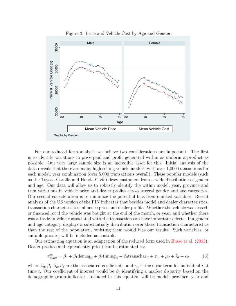
Figure 3: Price and Vehicle Cost by Age and Gender

2000

025

000

3000

035

000

20 40 60 80 20 40 60 80

Male Female

Mean Vehicle Price Mean Vehicle Cost

Pric

e &

Vehi

cle

Cos

t ($)

Age

Graphs by Gender

For our reduced form analysis we believe two considerations are important. The firstis to identify variations in price paid and profit generated within as uniform a product aspossible. Our very large sample size is an incredible asset for this. Initial analysis of thedata reveals that there are many high selling vehicle models, with over 1,000 transactions foreach model, year combination (over 5,000 transactions overall). These popular models (suchas the Toyota Corolla and Honda Civic) draw customers from a wide distribution of genderand age. Our data will allow us to robustly identify the within model, year, province andtrim variations in vehicle price and dealer profits across several gender and age categories.Our second consideration is to minimize the potential bias from omitted variables. Recentanalysis of the US version of the PIN indicates that besides model and dealer characteristics,transaction characteristics influence price and dealer profits. Whether the vehicle was leased,or financed, or if the vehicle was bought at the end of the month, or year, and whether therewas a trade-in vehicle associated with the transaction can have important effects. If a genderand age category displays a substantially distribution over these transaction characteristicsthan the rest of the population, omitting them would bias our results. Such variables, orsuitable proxies, will be included as controls.

Our estimating equation is an adaptation of the reduced form used in Busse et al. (2013).Dealer profits (and equivalently price) can be estimated as:

πmidgpt = β0 + β1demogit + β2timingit + β3transcharit + τm + µd + λt + εit (3)

where β0, β1, β2, β3 are the associated coefficients, and εit is the error term for individual i attime t. Our coefficient of interest would be β1 identifying a market disparity based on thedemographic group indicator. Included in this equation will be model, province, year and

11

Figure 4: Customer Age Distribution for Popular Models

Civic Corolla

Escape Yaris

0

1000

2000

3000

4000

0

1000

2000

3000

4000

25 50 75 25 50 75Customer Age

Num

ber

Sol

d

trim fixed effects τm, dealer fixed effects µd and time fixed effects λt. This equation will yieldthe average within model-province-year-trim difference in dealer margin across our genderand age categories.

For illustration, assume that in our dataset we have two models: a Honda Civic, and aToyota Corolla, two provinces: Ontario, and Quebec, two years: 2008 and 2009, and finallytwo demographic categories: male and female. The average difference in dealer margin acrossmales and females for a Honda Civic sold in Ontario in 2008 would be a part of our estimate.The estimate generated by our equation, further averages this average difference across malesand females over each of the 8 possibilities in the combinations above.

3.3 The reasons for market disparities across gender and age.

On discovering market disparities across gender and age groups how are we to interpret them.Are differences in dealer prices due to statistical or taste based discrimination? The possibil-ities of statistical discrimination are several. A variation in price elasticity, and preferencesacross gender and age could explain the difference in market outcomes observed. Giventhe importance of negotiation in the market, an inherent difference in bargaining strategiesacross gender (see Babcock and Laschever (2003)) could yield differences. Differences insearch costs—through internet access, or a propensity to research vehicles—across genderand age could influence market outcomes (similar to Morton et al. (2003)).

A taste based explanation for differences in market outcomes derives from differences inthe utility derived from interacting with different groups. For instance, a male dominatedcar salesman might prefer interacting with a young female customer and be willing to accepta smaller profit from that transaction.

12

Table 6: Regression of Log(Vehicle Cost)

(1) (2) (3)Female -0.123a (0.001) -0.000 (0.000) 0.003a (0.000)Age 25-30 0.091a (0.002) 0.003a (0.001) 0.003a (0.001)Age 30-35 0.162a (0.002) 0.005a (0.001) 0.006a (0.001)Age 35-40 0.201a (0.002) 0.007a (0.001) 0.008a (0.001)Age 40-45 0.202a (0.002) 0.007a (0.001) 0.008a (0.001)Age 45-50 0.188a (0.002) 0.008a (0.001) 0.008a (0.001)Age 50-55 0.180a (0.002) 0.009a (0.001) 0.009a (0.001)Age 55-60 0.184a (0.002) 0.010a (0.001) 0.010a (0.001)Age 60-65 0.183a (0.003) 0.009a (0.001) 0.011a (0.001)Age 65-70 0.160a (0.003) 0.005a (0.001) 0.010a (0.001)Age > 70 0.117a (0.003) -0.000 (0.001) 0.008a (0.001)Financed Indicator -0.033a (0.001) 0.019a (0.001) 0.022a (0.000)Leased Indicator 0.031a (0.001) 0.027a (0.001) 0.029a (0.000)Sat or Sun FE -0.005a (0.001) -0.001a (0.001) -0.001b (0.000)End of Month FE 0.015a (0.001) -0.001a (0.000) -0.001a (0.000)End of Year FE 0.010b (0.004) -0.001 (0.002) -0.001 (0.001)Constant 9.987a (0.007) 10.223a (0.003) 10.199a (0.002)R2 0.171 0.896 0.935c p < 0.1, b p < 0.05, a p < 0.01. Fixed-effects specified as Col. 1: Province; Col. 2:Model-Year-Province; Col. 3: Model-Year-Trim-Province. All regressions include year-month FEs. N=510866.

A combination of several factors likely explains observed market disparities in the newautomobile market. It is unlikely that we will have a certain answer on the relative con-tribution of different explanations. While our research will look for associated evidence forvarious explanations, that will not be its primary goal.

4 Regression Results

We now present results from estimating Equations XX and XXX in the previous section.

4.1 Regressions of Vehicle Cost

We first examine how the age and gender of consumers relates to vehicle costs. Table 6regresses the log of the vehicle cost, as recorded by the dealer, on demographic character-istics. Column 1 includes fixed-effects for the province of the transaction. Column 2 usesModel*model-year*province fixed-effects, and Column 3 uses Model*model-year*trim*provincefixed-effects. All regressions include year-month fixed-effects to control for general trends invehicle prices. The first column reveals the relationship between age and gender and averagenew car prices, without controlling for the make or model or trim-level of the car. The omit-ted age category is consumers aged below 25. Thus the results in column 1 show that the

13

youngest consumers buy the cheapest cars. Consumers aged 25-30 buy 10% more expensivecars on average, and the premium is about 18–20% for the other age groups. Consumersaged 70 and above buy less expensive cars than consumers in all age categories between 30and 70.

Column 2 of Table 6 shows that, once we control for the vehicle model, there are nolonger large differences across age groups. While the very youngest and oldest consumerspurchase less expensive trims, the difference between these consumers and the rest is at mostone percent. A similar pattern in column 3 shows that there is no clear relationship betweencustomer age and aftermarket options or warranties, other than evidence that consumersunder the age of 30 are the least likely to make such purchases.

Column 1 shows that female consumers buy new cars that are 12% cheaper on averagethan those bought by male consumers. However, this difference completely disappears oncewe control for model in Column 2, indicating that gender has no relationship with vehicletrim within a given model. Column 3 suggests that female consumers spend slightly moreon options and warranties than men do, although the difference of 0.3% is economically verysmall despite being statistically significant.

We also include indicators for the timing of the transaction, and whether the vehicle wasleased or financed through the dealer. Column 1 shows that consumers who finance theirvehicles tend to buy cheaper cars. However, once we control for make in column 2 and trimin column 3, consumers who finance tend to buy more expensive vehicles. A similar effectis seen for consumers who lease vehicles. Weekends see the sales of slightly cheaper vehicleson average, although once make and trim are controlled for, the effect is tiny. On average,slightly more expensive vehicles are sold at the end of the month and the year, but againthe effects are small or non-existent when we control for model and trim.

In Table 7 we examine the joint distribution of age and gender, using the same sets offixed-effects as in the previous table. The omitted category is male consumers under theage of 25. The results in column 1 show that in every age category, female consumers buycheaper cars on average than their male counterparts of the same age, showing that theprevious result regarding gender holds across age groups. Indeed the male-female new carpremium is a remarkably robust 13–16% in almost every age category. Young women buy thecheapest cars of any gender-age group, while 35 to 65 year old men buy the most expensivecars.

The large coefficients that we observe in column 1 of Table 7 disappear in column 2,which controls for the model purchased. Thus, there appears to be no systematic relation-ship between customer demographics and the choice of trims within a given model, just aswe saw in Table 6. In column 3, the coefficients on each demographic group are positive andstatistically significant, indicating that men under the age of 25 spend the least on aftermar-ket options and warranties. Examining the coefficients suggests that, beyond the age of 40,women spend slightly more on these add-ons than men of the same age, but the differencesare small.

Our results so far indicate that consumer demographics are systematically related to thepurchase price of the vehicle, but that this is almost entirely due to choices regarding whichmake and model to purchase. Conditional on the model, demographics do not have a clearrelationship with consumers’ choice of vehicle trims or other options. We now turn to thequestion of how consumers’ characteristics relate to dealer profits.

14

Table 7: Regression of Log(Vehicle Cost)

(1) (2) (3)Age < 25 Female -0.157a (0.004) -0.007a (0.001) 0.003a (0.001)Age 25-30 Male 0.077a (0.003) 0.001 (0.001) 0.005a (0.001)Age 25-30 Female -0.054a (0.003) -0.004a (0.001) 0.005a (0.001)Age 30-35 Male 0.140a (0.003) 0.003a (0.001) 0.008a (0.001)Age 30-35 Female 0.027a (0.004) -0.002c (0.001) 0.006a (0.001)Age 35-40 Male 0.174a (0.003) 0.004a (0.001) 0.009a (0.001)Age 35-40 Female 0.074a (0.003) 0.003b (0.001) 0.010a (0.001)Age 40-45 Male 0.182a (0.003) 0.004a (0.001) 0.009a (0.001)Age 40-45 Female 0.065a (0.003) 0.003b (0.001) 0.010a (0.001)Age 45-50 Male 0.169a (0.003) 0.004a (0.001) 0.008a (0.001)Age 45-50 Female 0.049a (0.003) 0.005a (0.001) 0.011a (0.001)Age 50-55 Male 0.160a (0.003) 0.003b (0.001) 0.008a (0.001)Age 50-55 Female 0.043a (0.003) 0.007a (0.001) 0.014a (0.001)Age 55-60 Male 0.169a (0.003) 0.005a (0.001) 0.009a (0.001)Age 55-60 Female 0.039a (0.004) 0.007a (0.001) 0.015a (0.001)Age 60-65 Male 0.173a (0.003) 0.005a (0.001) 0.010a (0.001)Age 60-65 Female 0.029a (0.004) 0.006a (0.001) 0.015a (0.001)Age 65-70 Male 0.146a (0.004) -0.001 (0.001) 0.008a (0.001)Age 65-70 Female 0.014a (0.004) 0.004b (0.002) 0.016a (0.001)Age > 70 Male 0.099a (0.003) -0.006a (0.001) 0.007a (0.001)Age > 70 Female -0.025a (0.004) -0.001 (0.002) 0.015a (0.001)Financed Indicator -0.034a (0.001) 0.019a (0.001) 0.022a (0.000)Leased Indicator 0.031a (0.001) 0.027a (0.001) 0.029a (0.000)Sat or Sun FE -0.005a (0.001) -0.001a (0.001) -0.001b (0.000)End of Month FE 0.015a (0.001) -0.001a (0.000) -0.001a (0.000)End of Year FE 0.010b (0.004) -0.001 (0.002) -0.001 (0.001)Constant 10.005a (0.008) 10.226a (0.003) 10.199a (0.002)R2 0.171 0.896 0.935c p < 0.1, b p < 0.05, a p < 0.01. Fixed-effects specified as Col. 1: Province; Col. 2:Model-Year-Province; Col. 3: Model-Year-Trim-Province. All regressions include year-month FEs. N=510866.

15

Table 8: Regression of Dealer Margin

(1) (2) (3)Female -107.6a (3.9) 13.0a (3.6) 21.5a (3.6)Age 25-30 107.5a (10.0) 6.5 (9.1) 8.4 (9.0)Age 30-35 178.0a (9.8) 6.7 (9.0) 8.5 (9.0)Age 35-40 224.6a (9.6) 23.2a (8.9) 26.5a (8.9)Age 40-45 254.7a (9.3) 45.1a (8.6) 48.1a (8.6)Age 45-50 269.5a (9.2) 68.6a (8.5) 71.8a (8.5)Age 50-55 281.2a (9.4) 84.8a (8.6) 87.4a (8.6)Age 55-60 282.7a (9.8) 84.5a (9.0) 88.9a (9.0)Age 60-65 257.4a (10.6) 79.5a (9.7) 83.9a (9.7)Age 65-70 232.3a (11.7) 98.6a (10.8) 105.2a (10.8)Age > 70 194.0a (10.8) 130.1a (10.1) 144.4a (10.1)Financed Indicator -44.0a (6.1) 171.5a (5.8) 180.4a (5.8)Leased Indicator 36.3a (6.0) 185.5a (5.7) 198.0a (5.7)Sat or Sun FE 20.4a (6.1) 22.3a (5.5) 23.1a (5.5)End of Month FE -40.5a (4.4) -60.0a (4.0) -61.0a (4.0)End of Year FE -88.1a (17.9) -93.2a (16.2) -93.6a (16.2)Constant 1607.8a (31.0) 2384.5a (26.7) 2360.3a (26.9)R2 0.037 0.239 0.264c p < 0.1, b p < 0.05, a p < 0.01. Fixed-effects specified as Col. 1: Province;Col. 2: Model-Year-Province; Col. 3: Model-Year-Trim-Province. Allregressions include year-month FEs. N=510866.

4.2 Regressions of Dealer Margin

The results are presented in Table 8, where the dependent variable is the dealer’s margin oneach transaction. Note that we do not take logs of this variable because dealer margins arenegative in about 8% of cases, which would require us to drop these observations.8 Column 1shows that dealers make on average $107 less on female consumers, as well as lower marginson younger consumers. A 45 to 65 year old consumer generates about $280 higher dealermargins than a consumer under 25, and about $100 more than those between 25 and 30.But this is not surprising, given the same pattern with regard to the kinds of cars theseconsumers buy, as shown in Table 6. That is, dealers make their lowest margins on thecheapest cars. More interesting are the results in the other two columns. Column 2, whichcontrols for model, reveals that dealers generate slightly higher margins on female consumersand considerably higher margins on older consumers — as much as $100–130 on consumersabove the age of 65. There differences persist, and are in fact somewhat larger, in column3, which also controls for vehicle trim. Consumers above 65 generate about $105–144 highermargins for dealers than consumers under the age of 35.

8As discussed above, dealers make negative margins for a number of reasons, including responding tomanufacturer incentives, getting rid of cars with low demand, and taking losses on the new car in order tomake profits on the trade-in. Below, we show that our results are fully robust to using only transactionswith positive dealer margins, and expressing the dependent variable in logs.

16

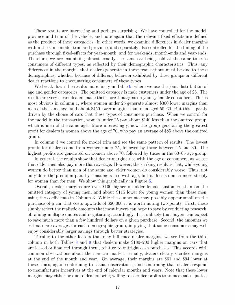
These results are interesting and perhaps surprising. We have controlled for the model,province and trim of the vehicle, and note again that the relevant fixed effects are definedas the product of these categories. In other words, we examine differences in dealer marginswithin the same model-trim and province, and separately also controlled for the timing of thepurchase through fixed-effects for year-month, and for weekends, month-ends and year-ends.Therefore, we are examining almost exactly the same car being sold at the same time toconsumers of different types, as reflected by their demographic characteristics. Thus, anydifferences in the margins that dealers generate in these transactions must be due to thesedemographics, whether because of different behavior exhibited by these groups or differentdealer reactions to encountering consumers of these types.

We break down the results more finely in Table 9, where we use the joint distribution ofage and gender categories. The omitted category is male customers under the age of 25. Theresults are very clear: dealers make their lowest margins on young, female consumers. This ismost obvious in column 1, where women under 25 generate almost $300 lower margins thanmen of the same age, and about $450 lower margins than men aged 50–60. But this is partlydriven by the choice of cars that these types of consumers purchase. When we control forthe model in the transaction, women under 25 pay about $140 less than the omitted group,which is men of the same age. More interestingly, now the group generating the greatestprofit for dealers is women above the age of 70, who pay an average of $85 above the omittedgroup.

In column 3 we control for model trim and see the same pattern of results. The lowestprofits for dealers come from women under 25, followed by those between 25 and 30. Thehighest profits are generated on women above 70, followed by those in the 60–65 age group.

In general, the results show that dealer margins rise with the age of consumers, as we seethat older men also pay more than average. However, the striking result is that, while youngwomen do better than men of the same age, older women do considerably worse. Thus, notonly does the premium paid by consumers rise with age, but it does so much more steeplyfor women than for men. We show this graphically in Figure 5.

Overall, dealer margins are over $100 higher on older female customers than on theomitted category of young men, and about $115 lower for young women than these men,using the coefficients in Column 3. While these amounts may possibly appear small on thepurchase of a car that costs upwards of $20,000 it is worth noting two points. First, thesesimply reflect the realistic amounts that most buyers can hope to save by conducting research,obtaining multiple quotes and negotiating accordingly. It is unlikely that buyers can expectto save much more than a few hundred dollars on a given purchase. Second, the amounts weestimate are averages for each demographic group, implying that some consumers may wellenjoy considerably larger savings through better strategies.

Turning to the other factors that may influence dealer margins, we see from the thirdcolumn in both Tables 8 and 9 that dealers make $180–200 higher margins on cars thatare leased or financed through them, relative to outright cash purchases. This accords withcommon observations about the new car market. Finally, dealers clearly sacrifice marginsat the end of the month and year. On average, their margins are $61 and $94 lower atthese times, again conforming to casual observations, and confirming that dealers respondto manufacturer incentives at the end of calendar months and years. Note that these lowermargins may either be due to dealers being willing to sacrifice profits to to meet sales quotas,

17

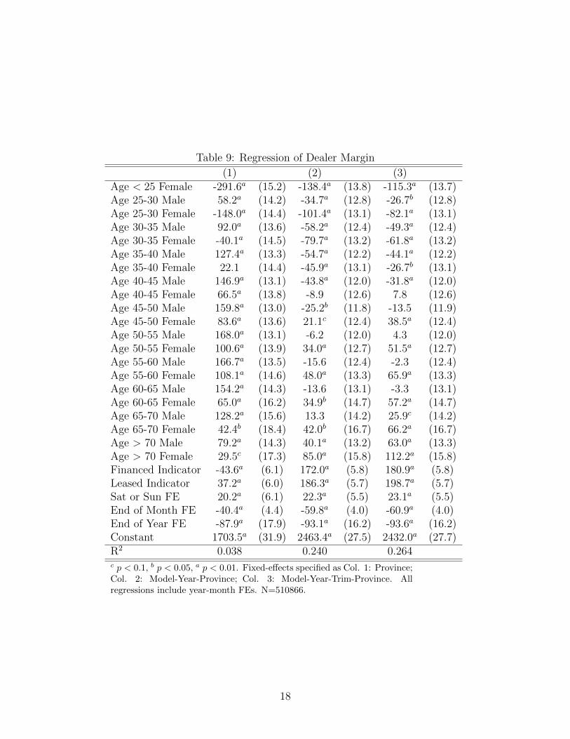
Table 9: Regression of Dealer Margin

(1) (2) (3)Age < 25 Female -291.6a (15.2) -138.4a (13.8) -115.3a (13.7)Age 25-30 Male 58.2a (14.2) -34.7a (12.8) -26.7b (12.8)Age 25-30 Female -148.0a (14.4) -101.4a (13.1) -82.1a (13.1)Age 30-35 Male 92.0a (13.6) -58.2a (12.4) -49.3a (12.4)Age 30-35 Female -40.1a (14.5) -79.7a (13.2) -61.8a (13.2)Age 35-40 Male 127.4a (13.3) -54.7a (12.2) -44.1a (12.2)Age 35-40 Female 22.1 (14.4) -45.9a (13.1) -26.7b (13.1)Age 40-45 Male 146.9a (13.1) -43.8a (12.0) -31.8a (12.0)Age 40-45 Female 66.5a (13.8) -8.9 (12.6) 7.8 (12.6)Age 45-50 Male 159.8a (13.0) -25.2b (11.8) -13.5 (11.9)Age 45-50 Female 83.6a (13.6) 21.1c (12.4) 38.5a (12.4)Age 50-55 Male 168.0a (13.1) -6.2 (12.0) 4.3 (12.0)Age 50-55 Female 100.6a (13.9) 34.0a (12.7) 51.5a (12.7)Age 55-60 Male 166.7a (13.5) -15.6 (12.4) -2.3 (12.4)Age 55-60 Female 108.1a (14.6) 48.0a (13.3) 65.9a (13.3)Age 60-65 Male 154.2a (14.3) -13.6 (13.1) -3.3 (13.1)Age 60-65 Female 65.0a (16.2) 34.9b (14.7) 57.2a (14.7)Age 65-70 Male 128.2a (15.6) 13.3 (14.2) 25.9c (14.2)Age 65-70 Female 42.4b (18.4) 42.0b (16.7) 66.2a (16.7)Age > 70 Male 79.2a (14.3) 40.1a (13.2) 63.0a (13.3)Age > 70 Female 29.5c (17.3) 85.0a (15.8) 112.2a (15.8)Financed Indicator -43.6a (6.1) 172.0a (5.8) 180.9a (5.8)Leased Indicator 37.2a (6.0) 186.3a (5.7) 198.7a (5.7)Sat or Sun FE 20.2a (6.1) 22.3a (5.5) 23.1a (5.5)End of Month FE -40.4a (4.4) -59.8a (4.0) -60.9a (4.0)End of Year FE -87.9a (17.9) -93.1a (16.2) -93.6a (16.2)Constant 1703.5a (31.9) 2463.4a (27.5) 2432.0a (27.7)R2 0.038 0.240 0.264c p < 0.1, b p < 0.05, a p < 0.01. Fixed-effects specified as Col. 1: Province;Col. 2: Model-Year-Province; Col. 3: Model-Year-Trim-Province. Allregressions include year-month FEs. N=510866.

18

Figure 5: Dealer Margin premium for demographic groups, relative to Men under 25

−100

−50

0

50

100

<25 25−30 30−35 35−40 40−45 45−50 50−55 55−60 60−65 65−70 75+Age Group

Dea

ler

Mar

gin

Gender

female

male

or by more price-conscious consumers negotiating transactions at these times, knowing theincentives dealers face.

4.3 Robustness Regressions

Below, we will discuss the possible reasons for our results on particular demographic groups.First, though, we present evidence that the results are not driven by other factors, such asomitted variables, outlier observations, or selection. The regression results for the followingexercises are presented in Tables 10, 11 and 12 in the Appendix. We present the maincoefficients of interest more compactly in Figure 6. Note that these results are obtainedfrom regressions using the same specification as Column 3 of Table 9, which include fixedeffects for model-year-province-trim and for year-months.

We start by examining particular segments — Compact cars, SUVs and Vans in PanelsA and B. These segments are disproportionately associated with particular age groups, aswe saw in Section 2; younger consumers are more likely to purchase small cars, while middle-aged consumers, especially those that are married, are more likely to purchase family carssuch as SUVs and minivans. We then show, in Panel C, that our results are robust toexamining only popular car models; i.e. that they are not driven by unusual consumer ordealer behavior in vehicles with low sales. We define high-selling car models as those withat least 5000 units in sales during our sample period. This corresponds to 26 models, out ofour observed set of more than 500 models, and these comprise almost 50% of total vehiclesales.

Next, we consider the possibility that new vehicle transaction prices may be influencedby the amounts negotiated on consumers’ trade-in vehicles. While in principle the twotransactions should be treated separately, in practice dealers may allow overpayment on

19

Figure 6: Dealer Margin premium for subsamples, relative to Men under 25

A: Compacts B: SUVs+Vans C: High−selling

D: No Trade−ins E: Positive Margins F: Dealer Controls

−200

−100

0

100

−200

−100

0

100

25−30 40−45 55−60 70+ 25−30 40−45 55−60 70+ 25−30 40−45 55−60 70+Age Group

Dea

ler

Mar

gin

Gender

female

male

some trade-ins in order to make greater margins on the new car, or vice versa.9 We thereforerestrict attention, in Panel D of Figure 6, to the subset of transactions where consumers didnot trade-in an older vehicle. We then restrict the sample, in Panel E, to those where dealersmake positive margins on new car sales. While we have explained above that there may berational reasons for dealers to make losses on certain transactions, one may be concernedthat these sales are specific to certain types of cars or to unobserved characteristics of thetransaction which may be correlated with consumer demographics.

Finally, we control for systematic pricing behavior by certain dealers. Suppose, for ex-ample, that dealers located in smaller cities or suburban locations charge lower prices forexactly the same car as a city dealer who faces higher costs. If the demographic distributionof consumers in these two locations is also different — for example, if older consumers aremore likely to live near high-cost dealers — then this selection of consumer types may driveour results. We can control for this possibility by including dealer fixed-effects, which allowus to look within dealers. We also include the number of days that the vehicle has been onthe dealer’s lot — popular cars typically turnover very quickly and so dealers may be willingto reduce margins on cars that are not in high demand. The coefficients are presented inPanel F of Figure 6.

All six panels support our overall finding that dealer margins rise with consumer age;this is a very robust result. With regard to our second main result — that the age premiumrises more steeply for women than for men — we also find considerable support. In all

9See Zhu et al. (2008) for evidence regarding this possibility.

20

six panels, the blue line corresponding to the female premium starts below the red linecorresponding to the male premium, and ends up above it. However, this result is lessrobust in some subsamples. The gender gap among older consumers is quite small when weexamine compacts alone in Panel A. In addition, the coeffcients for older women are notalways significantly different from zero in Panel B (see Column 2 of Table 10 for detailedresults and standard errors). Generally, though, the finding regarding differential age effectsby gender is confirmed.

5 Discussion of results

In this section we discuss some possible explanations for the regression results obtained inSection 4. Recall our two main findings: first, dealers generally make higher margins onolder consumers. Second, the age premium rises more steeply for women than for men; as aresult, young women pay the least for new cars, whereas older women pay the most.

We first discuss the finding of a secular correlation between customer age and dealermargin.10 Recall that our results are obtained from the period 2004–2009, and so essentiallyrepresent a snapshot of the new car market at a particular point of time. Therefore, wecannot say with certainty whether this result will hold continuously, or is particular to thetime period that we examine. In other words, the result may either represent an ongoingeffect, in which case we should expect older consumers to continuously fare worse in the newcar market, or it may be a cohort effect, which is particular to the set of consumers thatwere observed during this period.

If the ongoing effect is true — i.e. if older consumers simply do worse in price negotiations— then we would expect this result to be repeated in future studies as well. In particular,we would expect the young consumers of today, who currently negotiate the lowest prices,to do worse as they age. By contrast, if the cohort effect is true, then there is somethingparticular about the current generation of older consumers that leads them to fare worse inthe new car market, but this fact may not continue to hold for future generations.

Both explanations may have some support. We know from prior research (Morton et al.(2011)) that search costs are important in price negotiations for new cars. It is possible thatyounger consumers have the lowest search costs and that search costs rise with the age ofconsumers. However, it is perhaps a little counter-intuitive to think of consumers above 65as having the highest search costs, as these consumers are most likely to be retired or out ofthe labor force.

Prior research has also shown that research on the Internet can reduce the prices thatconsumers pay for new cars. (Morton et al. (2001)) show that consumers using an onlinereferral service can do better than a majority of other users. Since that study, there havebeen a host of new sources of information on new car sales. Websites such as Carfax.comand Edmunds.com provide consumers with detailed information about the invoice priceof particular vehicles, suggesting that the savings from online research may have grownconsiderably. Separately, there is clear evidence that older consumers are less likely to use

10Note that a similar finding was obtained by Harless and Hoffer (2002), although they did not break downtheir result by gender. Moreover, that study used a much smaller sample than ours, and did not control forother factors such as idiosyncratic dealer behavior, trade-in vehicles, etc.

21

the Internet (cite StatsCan data). If this is true then the age effects we estimate may reflectexisting gaps in online use between old and young consumers, but these may not persist asthe current cohort of young users — who are comfortable going online — grows older.

We now turn to the differential age effects by gender. Ours is the first study to identifythis effect and as with the first finding there is no clear explanation. However, we believe itis unlikely that this result is an ongoing effect: there is no good reason to expect that theyoung women of today, who are negotiating better autombile prices than men of the sameage, will in the future start to do worse than these same men. In other words, if we treatmale consumers as a control group, then the results are evidence that there is somethingdifferent about young women in our sample compared to older women.

Our explanation builds on the very different labor market experiences and educationattainment of women in the under 30 cohort versus those in their 60s and above. It is wellknown that over the past few decades, women in North America have considerably narrowedthe education gap with men, and in recent years have even surpassed men. At the sametime, women’s labor force participation has grown rapidly.

The economic effects of these societal changes are important, and potentially explain ourfindings. Most prior research on these economic consequences has focused on labor marketoutcomes — most importantly, on women’s wages. Research has shown that while there hasbeen some reduction in the pay gap, women still earn less than men in similar occupations.There is considerably less research on the impacts this has had on other economic outcomes,particularly on price negotiations.

Our results are consistent with the idea that the better educational attainment and laborforce participation of young women, relative to men of the same age, may lead to thesewomen performing better in price negotiations. Women above the age of 65 are much lesslikely to have completed high-school or college, or to have been employed full-time when theywere younger. Another subtle explanation for our results may be the effects of marriage.The data show that women above 65 are more likely to be single than those in their 30s and40s, due to the effects of divorce as well as higher death rates for men in the same cohort.We believe it is likely that older women who buy new cars in our sample are more likely tobe entering the new car market on their own for the first time, possibly having participatedin it along with their spouses in the past. If so, these women may be at a disadvantage dueto never having negotiated before on their own for such a big-ticket item.

References

Ayres, I. and P. Siegelman (1995, June). Race and gender discrimination in bargaining fora new car. American Economic Review 85 (3), 304–21.

Babcock, L. R. and S. Laschever (2003). Women Don’t Ask: Negotiation and the GenderDivide. Princeton University Press.

Bertrand, M., C. Goldin, and L. F. Katz (2010). Dynamics of the gender gap for youngprofessionals in the financial and corporate sectors. American Economic Journal: AppliedEconomics , 228–255.

22

Bertrand, M. and K. F. Hallock (2001, October). The gender gap in top corporate jobs.Industrial and Labor Relations Review 55 (1), 3–21.

Blau, F. D. and L. M. Kahn (2007). The gender pay gap have women gone as far as theycan? The Academy of Management Perspectives 21 (1), 7–23.

Busse, M. R., C. R. Knittel, and F. Zettelmeyer (2013). Are consumers myopic? evidencefrom new and used car purchases. The American Economic Review 103 (1), 220–256.

Goldberg, P. K. (1996, June). Dealer price discrimination in new car purchases: Evidencefrom the consumer expenditure survey. Journal of Political Economy 104 (3), 622–54.

Harless, D. W. and G. E. Hoffer (2002, March). Do women pay more for new vehicles?evidence from transaction price data. American Economic Review 92 (1), 270–279.

Lang, K. and J.-Y. K. Lehmann (2012). Racial discrimination in the labor market: Theoryand empirics. Journal of Economic Literature 50 (4), 959–1006.

Langer, A. (2011). Demographic preferences and price discrimination in new vehicle sales.manuscript, University of Michigan.

List, J. A. (2004, February). The nature and extent of discrimination in the marketplace:Evidence from the field. The Quarterly Journal of Economics 119 (1), 49–89.

Morton, F. S., J. Silva-Risso, and F. Zettelmeyer (2011). What matters in a price negotiation:Evidence from the us auto retailing industry. Quantitative Marketing and Economics 9 (4),365–402.

Morton, F. S., F. Zettelmeyer, and J. Silva-Risso (2001). Internet car retailing. The Journalof Industrial Economics 49 (4), 501–519.

Morton, F. S., F. Zettelmeyer, and J. Silva-Risso (2003). Consumer information and dis-crimination: Does the internet affect the pricing of new cars to women and minorities?Quantitative Marketing and Economics 1 (1), 65–92.

O’Neill, J. (2003). The gender gap in wages, circa 2000. The American Economic Re-view 93 (2), 309–314.

Stuhlmacher, A. F. and A. E. Walters (1999). Gender differences in negotiation outcome: Ameta-analysis. Personnel Psychology 52 (3), 653–677.

Yinger, J. (1998, Spring). Evidence on discrimination in consumer markets. Journal ofEconomic Perspectives 12 (2), 23–40.

Zhu, R., X. Chen, and S. Dasgupta (2008). Can trade-ins hurt you? exploring the effectof a trade-in on consumers’ willingness to pay for a new product. Journal of MarketingResearch 45 (2), 159–170.

23