The Geiger-Muller Tube and Particle Counting

• Abstract:– Emissions from a

radioactive source were used, via a Geiger-Muller tube, to investigate the statistics of random events. Unexpected difficulties were encountered and overcome.

• Collaborators– Michael J. Sheldon (sfsu)

– Justin Brent Runyan (sfsu)

Overview

• Background– Statistics

• Poisson / Gaussian distribution functions

– equipment and methods

• Initial Results

• What went wrong?– Speculation

– A workable hypothesis

• The search for a solution

• Conclusion

Poisson Distribution Function

• Conditions for Use– You Have n independent trials.– The probability (p) of any particular outcome is

the same for all trials.– n is large and p is small

• The Poisson function says:– f(x, ) = ^x* e^- / x!– Where = np

Gaussian Distribution Function

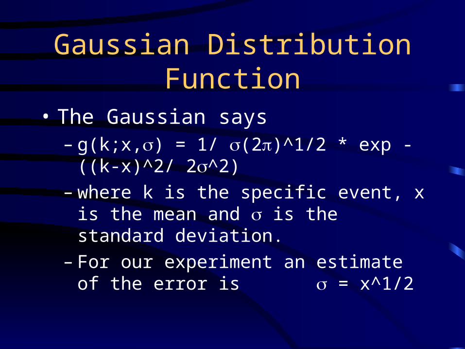
• The Gaussian says– g(k;x,) = 1/ (2)^1/2 * exp -((k-x)^2/ 2^2)– where k is the specific event, x is the mean and

is the standard deviation.– For our experiment an estimate of the error is

= x^1/2

Equipment and Methods

• Source of random events: Gamma Radiation from Co-60

• Co-60 has long half life compared to the length of the experiment

• # of emissions/t is random

Equipment and Methods

• G-M tube allows observation of -ray emissions

• Tube is filled with low pressure gas which is ionized when hit with radiation.

• G-M tube sends week pulse to interface.

Equipment and Methods

• The interface beefs up G-M tube signal for computer.

• Caused problems for us.

Equipment and Methods

• Signal from interface fed into computer.

• We counted number of emissions in given time intervals.

• Data was analyzed with scientist, graphs created with excel and MINSQ.

• We tested statistical theories: = x^1/2 , fit of Gaussian/ Poisson dist. Functions etc...

Initial Results

• To see if = x^1/2 we did several runs with t = 10 sec

• Our results were not so hot.• However multiplying by 2^1/2 helped?

Run # of sources # of intervals X (mean) X^1/2

1 2 19 341 18

2 4 57 385 20

3 2 21 285 16

4 2 35 275 17

Initial Results: Gaussian dist.

• Obviously something is wrong

• There are two Gaussian dist. One for even bins one for odd.

• The even dist. Is larger than the odd.

Histogram

0

10

20

30

40

50

60

70

80

Bin

Frequency

Initial Results: Poisson Dist.

• Again the distribution function dose not exactly fit

• It is to skinny and to tall.

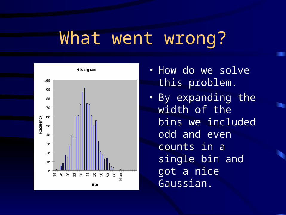
What went wrong?

• How do we solve this problem.

• By expanding the width of the bins we included odd and even counts in a single bin and got a nice Gaussian.

Histogram

0

10

20

30

40

50

60

70

80

90

100

14

20

26

32

38

44

50

56

62

68

More

Bin

Frequency

What Went Wrong?

• By replacing k with k/2 in the Poisson dist. We were able to make it fit better.

Speculation: What’s really going on?

• Brent speculated that the radiation from the source was coming out in pairs so that usually both particles made it into the detector and we got even numbers of counts.

• Pfr. Bland knocked this down.

• The real problem was that the computer was double counting the signal from the interface.

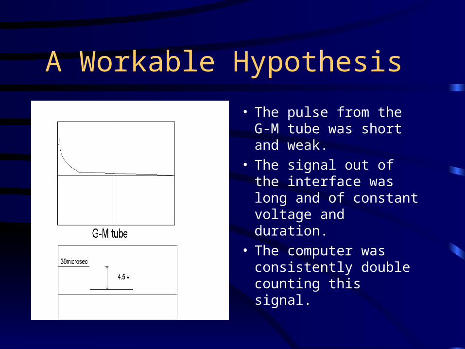
A Workable Hypothesis

• The pulse from the G-M tube was short and weak.

• The signal out of the interface was long and of constant voltage and duration.

• The computer was consistently double counting this signal.

The search for a solution.

• We knew that a capacitor was needed to round out the pulses from the interface.

• First we could not reproduce the problem.

• We could not get at the problem.

• The multitude of signal wires was confusing.

• We were desperate!!

Conclusion

• We had all given up when….

• The Magic combination was Blue to Yellow Green and Black.

• We were not able to run any simulations.

• Questions still remain about what line the signal ran on and why this combination worked.