WP/15/281

The Game of Anchors: Studying the Causes of Currency Crises in Belarus

By Alex Miksjuk, Sam Ouliaris, and Mikhail Pranovich

© 2015 International Monetary Fund WP/15/281

IMF Working Paper

Institute for Capacity Development

The Game of Anchors: Studying the Causes of Currency Crises in Belarus

Prepared by Alex Miksjuk, Mikhail Pranovich, and Sam Ouliaris1

Authorized for distribution by Ralph Chami

December 2015

Abstract

Belarus experienced a sequence of currency crises during 2009-2014. Our empirical results,

based on a structural econometric model, suggest that the activist wage policy and extensive

state program lending (SPL) conflicted with the tightly managed exchange rate regime and

suppressed monetary policy transmission. This created conditions for the unusually frequent

crises. At the current juncture, refocusing monetary policy from exchange rate to inflation

would help to avoid disorderly external adjustments. The government should abandon wage

targets and phase out SPL to remove the underlying source of the imbalances and ensure

lasting stabilization.

JEL Classification Numbers: C32, E42, E52, E61, F31, F41

Keywords: currency crisis, exchange rate policies, fiscal policy

Authors’ E-Mail Addresses: A.Miksyuk@nbrb.by; mpranovich@jvi.org; souliaris@imf.org

1 Alexei Miksjuk is a division chief at the National Bank of Belarus, Sam Ouliaris is a unit chief at the IMF

Institute for Capacity Development and Mikhail Pranovich is an economist at the Joint Vienna Institute. The

authors are grateful to Norbert Funke (JVI, Director) for supporting the scholar’s visit of Alexei Miksjuk to the

JVI in November 2014. The authors are grateful to Ralph Chami, Norbert Funke, Dmitry Murin, Martin

Schindler and the members of the IMF’s Belarus country team for comments and suggestions. We would like to

thank Thomas Chapman for help in formatting the paper. All remaining errors are the authors’ responsibility.

IMF Working Papers describe research in progress by the author(s) and are published to

elicit comments and to encourage debate. The views expressed in IMF Working Papers are

those of the author(s) and do not necessarily represent the views of the IMF, its Executive Board,

or IMF management.

Contents

I. Introduction ................................................................................................................................ 5

II. Overview of Macroeconomic Developments in Belarus: 2001-2014 ........................................ 6

III. Methodology of Research ........................................................................................................ 9

A. Long-Run Equilibrium Relationships .................................................................................. 10

B. Dynamic Econometric Model ............................................................................................... 11

C. State Program Lending ......................................................................................................... 12

D. Monetary Policy Regime in Belarus: Closing the Model ..................................................... 12

E. Modeling strategy ................................................................................................................. 16

IV. Model Estimation .................................................................................................................. 17

A. Data ...................................................................................................................................... 17

B. Estimating Long-Run Relationships ..................................................................................... 18

C. Estimating Short-Run Relationships .................................................................................... 19

D. Model Representation to Study Shocks: Ordering of Variables .......................................... 20

V. Impulse Response Analysis ..................................................................................................... 22

A. Monetary Policy Transmission: Policy Rate Shock ............................................................. 22

B. Monetary Policy Transmission: Exchange Rate Shock ........................................................ 23

C. Wage Shock .......................................................................................................................... 24

D. State Program Lending Shift ................................................................................................ 26

VI. Policy Discussion and Conclusion.......................................................................................... 28

References .................................................................................................................................... 32

Figures

1. BYR/USD depreciation ............................................................................................................. 7

2. Current account balance and financing ...................................................................................... 7

3. Current account balance structure .............................................................................................. 8

4. Investment in Belarus ................................................................................................................ 8

5. Growth of wages and productivity .............................................................................................. 9

6. Impulse response to 1pp policy rate shock .............................................................................. 22

7. Impulse response to 1 percent devaluation shock ..................................................................... 24

4

8. Impulse response to 1 percent wage shock ............................................................................... 25

9. Impulse response to 5 percent wage shock ............................................................................... 26

10. Impulse response to 1 percent SPL shift ................................................................................. 27

11. Impulse responses to 5 percent SPL shift ............................................................................... 28

Appendices

I. Long-Run Equilibrium Relationships ........................................................................................ 34

II. Data Description ....................................................................................................................... 37

III. Unit Root Test Results ............................................................................................................ 40

IV. Cointegration Test Results ...................................................................................................... 43

V. Estimated Reduced Form Model.............................................................................................. 44

VI. Impulse Responses to Demand, Inflation and Monetary Base Shocks .................................. 46

5

I. INTRODUCTION

By the beginning of 2000s, Belarus seemed to have settled on the main elements of its

macroeconomic policy. Monetary policy focused on the stability of the nominal exchange

rate, which was used as the nominal anchor. At the same time, to spur economic growth, the

government introduced a number of state investment programs. The aim was to increase

investment in sectors where the state remained a major stakeholder (agriculture, construction

and heavy industry). Another important pillar of the economic policy was setting “wage

objectives” that targeted the level of average wages. Moderating inflation and high economic

growth in the first eight years of 2000s seemed to prove that the chosen economic policy

worked. The 2009-2014 period, however, brought with it significant macroeconomic

destabilization, including three currency crises in 6 years.

In this paper, we develop a macro-econometric model to study the causes of currency crises.

After estimating the reduced-form model, we impose a structure that allows one to trace the

impact of structural shocks of different magnitudes to wages and state program lending

(SPL) on the economy and, in particular, on external balance.

Our main findings are the following:

the quasi-fiscal wage and SPL policies appear inconsistent with the chosen monetary

policy strategy based on the stabilized nominal exchange rate. We interpret this as a

policy conflict at the institutional level: putting in place an alternative rigid nominal

anchor (e.g., the wage level) and negating the efficiency of the exchange rate anchor;

despite the low degree of capital mobility in Belarus, the impact of monetary policy

via the interest rate channel remained weak, which contradicts the usual suggestion of

the “impossible trinity”. As widely discussed in the literature, such weakness may be

attributed to structural failures in the financial system. In the specific case of Belarus,

again, SPL could be the ultimate source suppressing market-based lending activity

and the steering role of interest rates;

the NBRB had little chance to defend the peg and withstand persistent increases in

nominal wages and/or SPL given the weak interest rate instrument and rather limited

foreign reserves. Ultimately, this led to unusually frequent currency crises. While

small shocks could be absorbed without exchange rate realignment, shocks with a

6

magnitude comparable to actual rates of increases in wages and SPL inevitably

induced a currency crisis. The latter underscores a rather low degree of economic

flexibility in Belarus.

These findings led us to two broadly unsurprising conclusions with respect to prevailing

macroeconomic policy framework:

adoption of a different monetary policy strategy with a more flexible nominal

exchange rate would limit the scope for crisis-like adjustment;

reducing and ultimately abandoning the activist wage policy and SPL would likely

remove the core root for currency crises and will create setup for lasting internal and

external stabilization.

In light of these recommendations, recent changes in macroeconomic policy – a plan to

reduce SPL, a switch to monetary targeting and managed floating exchange rate in 2015 – are

steps in the right direction.

The remainder of this paper is organized as follows. In the next section, we outline the key

macroeconomic developments in Belarus during 2001-2014. In Section III we discuss

methodology, model formulation and the estimation strategy. Section IV presents the data,

the reduced form estimation and the identification assumptions used to study shocks to the

economy. Section V describes the dynamic response of the economy to shocks to the

nominal exchange rate, the interest rate, nominal wages and the SPL – which provides the

basis for the policy discussion and recommendations presented in the final section.

II. OVERVIEW OF MACROECONOMIC DEVELOPMENTS IN BELARUS: 2001-2014

Like most transition economies in the region, after the turmoil of 1990s the Belarusian

economy enjoyed a strong recovery. In 2001-2008, average annual growth exceeded 8

percent, while the Belarusian rubel (exchange rate) was broadly stable. Inflation, though,

remained persistently high, falling below

10 percent y-o-y only three times during

the period. Figure 1: BYR/USD depreciation, q-o-q

7

The situation changed dramatically after

2008. The country suffered three crises

episodes in 6 years – in 2009, 2011 and

2014 (Figure 1). Prior to the each crisis,

the current account deficit widened to

more than 8 percent of GDP (Figure 2).

Authorities attempted to preserve

exchange rate stability through foreign

borrowing and FX interventions, which

resulted in significant (and rapid) foreign debt accumulation.

Figure 2: Current account balance and financing

A series of the negative terms of trade shocks in energy products in particular led to

deteriorating current account. Since 2007, however, energy trade deteriorated sharply as

Russia moved towards higher energy prices for Belarus. Moreover, foreign trade excluding

energy was also deteriorating, contributing to the imbalances, and net income payments

increased to service the growing foreign debt (Figure 3).2

2 Clearly, there were other shocks at play and figure 3 should be interpreted with caution. E.g., the shock to

build-up precautionary import took place prior to switching to VAT collection on the destination country

principle in trade with Russia in 2005. This shock deteriorated the current account deficit in 2004, but improved

the balance to unusually positive level in 2005.

8

Figure 3: Current account balance structure

The economy was slow to adjust to permanent energy shocks and external imbalances

remained persistent. To conjecture what prevented smooth adjustment of the economy to

equilibrium we now analyse the economic policy pursued by the Government and the NBRB.

State program lending

Active investment policy was at the heart

of the Belarusian economic growth model.

Investment to GDP ratio remained high,

with Belarus ranked around 10th

in the

world since 2008 (Figure 4).

State program lending (SPL) was the main

factor behind the investment surge. Banks

provided non-market SPL loans to selected

state-owned enterprises (SOEs). Although

the SPL stimulated investments and output

in the short-run, it also contributed to external and internal macroeconomic imbalances.3

3 The long-run effect of SPL on the economy is ambiguous. On one hand, SPLs speeded up capital

accumulation. On the other hand, the loans contributed to distorted capital allocation, so that total factor

productivity was declining (see Kruk and Haiduk (2013)).

Figure 4: Investment in Belarus

9

Activist wage policy

For most of 2000-2014, the Belarusian Government pursued activist wage policy by setting

wage targets. The government also had administrative instruments necessary to achieve these

targets, reflecting its dominant role in

economy.

Given standard spill-over effects to the

private sector, the official wage targets were

a key driver of wage dynamics in Belarus

(Koczan, 2014). Real wage growth (deflated

by CPI) exceeded productivity growth

(Figure 5). 4 This was likely a major cost-

push factor behind persistently high inflation

and the loss of price competitiveness.

Subordinated monetary policy and the case of (quasi-) fiscal dominance

The crises episodes of 2009, 2011 and 2014 resemble 1st generation of currency crises

(Krugman, 1979; Flood and Garber, 1984). The policy setup was that of fiscal dominance,

with a few important provisos. The government did not recognize the SPL in the budget

expenditures, which gave rise to a quasi-fiscal component of the deficit. The activist wage

policy was effectively a part of fiscal dominance: enterprises were directed to increase

wages, which created deficits in the real sector that eroded working capital and increased

demand for loans.

The quasi-fiscal policies substantially influenced the banking system and actions of the

NBRB. The SPL and rapid wage increases consequently spurred demand for loans primarily

supplied by the state-owned banks. In turn, this required timely closing of liquidity gaps and

therefore created an interest rate inelastic demand for reserve money. The NBRB refinanced

state-owned banks massively and in different forms: e.g., through liquidity provision at

4 For the most part, the additional income obtained from export price increases covered wage increases, which

implied that output prices were growing faster than CPI. Thus, real wage growth calculated using GDP deflator

was in line with output growth until 2011, implying stable share of labor costs in total income (Figure 5).

Figure 5: Growth of wages and productivity

10

subsidized rates and reduction of reserve requirements versus such banks, resulting in a

major increase in the money supply.

Such “refinancing” activities were at odds with the objective to preserve the exchange rate

and achieving moderate inflation with two important consequences. The NBRB had to, first,

extensively intervene in the FX market and, second, maintain high interest rates for the rest

of the economy. The FX interventions helped at times stabilize both the reserve money and

the exchange rate. However, as the official wage policy and SPL continued and the volume

of foreign reserves diminished, the exchange market faced intensified speculative attacks.

While the potential sources of imbalances are clear (e.g., IMF, 2015), the size of their impact,

their interaction and causality requires deeper analysis. We now construct a structural macro-

econometric model to understand and quantify these effects.

III. METHODOLOGY OF RESEARCH

Three important points need to be emphasized at this stage. First, we rely on macro-

econometric modelling. Second, we construct a structural model to study repeating currency

crises, investigate responses to shocks and the correction of the economy back to

equilibrium. We formulate a system of long-run economic relationships that together

describe a theoretically consistent Walrasian equilibrium for the economy. Our model

enforces long-run neutrality of monetary policy, stability of economy’s structure (shares of

GDP components) and debt solvency. Third, we keep the model as small as possible for

clarity of interpretation and for preserving estimation efficiency. However, the model should

be rich enough for the purposes of our research. The latter precludes us from strictly

following the structural cointegrating VAR approach as in Garrett et al. (2006), but we still

use it as the guiding principle.

A. Long-Run Equilibrium Relationships

We use the theoretical model that is similar to Garrett et al. (2006) in core, but with some

important differences (Appendix I). In the long-run, domestic output per capita grows in line

with foreign output per capita, implying similar technological progress. Relative prices are

11

determined by relative costs, with a Harrod-Balassa-Samuelson effect allowed for in the real

exchange rate. The standard exchange equation holds in the money market.

The key difference is in the foreign exchange market equilibrium. The UIP, balancing capital

flows, is a suitable equilibrium condition for advanced economies, but often proves

inadequate for emerging markets. Therefore, we model financial flows using a standard

portfolio balance approach by Branson and Henderson (1985) in which UIP deviations drive

private net foreign liabilities. Volumes and prices of trade flows are modelled among other

GDP expenditure components. The balance of payments identity takes trade and financial

flows together and defines changes in FX reserves.

To analyse the central bank policy tools, we consider the money supply explicitly and model

the money multiplier and the interest rate spread.

B. Dynamic Econometric Model

The dynamic model is in VECM form, namely:

tt

p

iititt

uxztcczx

*

1101

, (1)

supplemented with long-run identities

t

bb

t zx , (2)

where zt = (xt', xtb', xt

*')' is the full vector of variables, xt = (invt, const

pr, const

pu, ct

ex, ct

im, pt

inv,

pt, ptpu

, ptex

, ptim

, st, nflt, Rt, Rtib

, wt, mt, bt, invtGov

)' is the vector of endogenous variables. It

includes volumes of investment, private and public consumption, exports and imports, their

respective prices, the nominal exchange rate, net foreign liabilities of private sector, credit

and interbank real interest rates, nominal wages, money stock, monetary base and directed

loans disbursement to GDP. Vector xtb

= (yt, ct, pty, Intt)' collects endogenous variables that

are defined through balance identities and include output, absorption, GDP deflator and

central bank FX interventions vis-à-vis the private sector. Vector xt* includes n exogenous

variables. In (1), β is (22+n)r matrix comprising r cointegrating vectors (0 ≤ r ≤18), α is

18xr matrix of error correction coefficients, Λ is 18n matrix of coefficients of simultaneous

effect of exogenous variables. Matrices {Γi} are 18(22+n) of lagged effects, p is the lag

length, c0 is fixed intercept, c1 is the vector of deterministic trends, Γb is the matrix of

12

parameters for identities. Reduced form shocks are ut ~ iid(0, Σ) with 1818 covariance

matrix Σ.

Since Belarus is a small open economy, we treat xt* as strongly exogenous with respect to (1)

and do not specify a partial model for xt*, as it is not needed for impulse response analysis.

The long-run equilibrium relationships in Appendix I identify (2) and the 16 cointegrating

relationships reflected in β. The short-run dynamics is initially given by the unrestricted

VECM. Importantly, matrices α and β can have a maximum rank5 of 18, which is the number

of variables in xt. To fully identify the cointegrating vectors in β, we need to specify two

policy elements explicitly set by the authorities6: SPL and the nominal anchor. The form of

the specification (in levels or in differences) will determine the rank of the matrices (16, 17

or 18).

C. State Program Lending

As discussed in section II, SPL may be viewed as an economic policy tool used to boost

investments. SPL volumes are based on long-term state programs adopted by the

Government, but we found no regularity how the overall volume was determined. To model

SPL dynamics, we focus on budget constraints and expect the ratio of directed lending

disbursement to GDP (invtGov

) to be broadly stable, although we allow for linear trend in the

data, persistence (autocorrelation) in the process and a structural break in 2011Q2:

Gov

t

p

i

Gov

itigtbtb

Gov

t uinvxqdumtcxqdumctccinv

1

,,1,010 211211 . (3)

D. Monetary Policy Regime in Belarus: Closing the Model

Thus far all the long-run relationships in the model are expressed in real and relative-price

terms, ensuring long-run monetary policy neutrality. An equation for a nominal anchor needs

5 Since the vector zt comprises 22+n time series, there could be up to 21+ n cointegrating relationships. Up to 18

of these relationships may enter equation (1) in error-correction form

6 The other policy variables are subordinate (implicitly determined in the model) and endogenously react to

economic development.

13

to supplement these relationships. Choosing the appropriate anchor depends on the policy

strategy pursued by the central bank. De jure, the monetary policy regime in Belarus has

been subject to frequent changes. Instead, we consider de facto monetary policy regime.

An important input for identifying the policy regime in Belarus is imperfect capital mobility.

According to the “impossible trinity”, imperfect capital mobility allows for corner

possibilities of either inflation or exchange rate targeting. Yet another possibility is an

intermediate strategy with two objectives: exchange rate and inflation targeting as is

discussed in Ostry et al (2012).

The first corner option of inflation targeting and freely floating exchange rate does not seem

to be relevant, since the NBRB has always tightly controlled the BYR/USD exchange rate.

Therefore, a stabilized exchange rate is likely a part of one of the other two policy strategies.

If the NBRB targeted the exchange rate with no role for an inflation objective, then this

would imply no reaction of the short-term interest rate or reserve money to inflation. At least

one of the two conditions has to take place: (1) the NBRB used FX interventions to achieve

the exchange rate objective; (2) the NBRB used short-term domestic interest rates or reserve

money to achieve the exchange rate objective via affecting domestic money market

conditions.

The intermediate policy strategy would likely take place if, in addition to steering the

exchange rate, the NBRB attempted to adjust the interest rate in response to inflation

deviating from an explicit or implicit objective. This strategy would, of course, be sustainable

only if the inflation target (πt+) and the exchange rate target (devt

+) were chosen consistently:

πt+- devt

+ - Δpt

* = ∆qt

hp.

To close the model and empirically identify the policy strategy and policy implementation,

we formulate exchange rate, short-term-interest rate and domestic reserve money equations.

The exchange rate equation includes a linear trend to capture depreciation at a diminishing

rate in 2001-2003. It also allows for zero depreciation in 2004-2013Q2 (interrupted by two

currency crises episodes) and for roughly constant, positive rate of depreciation during

2013Q3-2014:

14

2011in ,

2014Q4-2013Q3in ,

excl.2011 2013Q2-2004Q1in 0,

2003Q4-2001Q1in ,

,4

,3

,1

,2

s

s

s

s

ttst

c

c

tc

ucriscs, (4)

Currency crises episodes are endogenous. We chose the interventions-to-reserves ratio

lagged one period to capture the timing of the crisis. The start of a crisis and step-devaluation

take place when this ratio exceeds a threshold 100 percent, which is equivalent to the amount

of previous period FX interventions being larger than the amount of foreign reserves

remaining in the end of that period.7 Devaluation is proportional to the size of real exchange

rate misalignment (cris t):

11

1111

if ,0

if ,

tt

tt

hp

tt

tIRA)(-Int

IRA)(-Intqqcris , (5)

where IRAt is the volume of foreign reserves, qthp

is the equilibrium real exchange rate.

Solving the monetary policy objective function gives the equation for the policy rate:8

,...

...)()(

1

*

,,1,0

11,411,311,21,1

ib

t

p

itibitibiibib

tib

spr

tibttibttibtib

ib

t

uxztcc

zyypIntyNR

(6)

where πt+ is the target inflation rate, ( tt yy ) is the domestic output gap (Appendix I).

Given (4), equation (6) allows for several strategies with a degree of control over the

exchange rate. The pure exchange rate targeting would be consistent with χ1,ib < 0, χ2,ib = 0

and χ3,ib = 0, while χ1,ib = 0 and χ2,ib > 0 should hold for the intermediate strategy. The latter

implies that the interest instrument focused on inflation and fully sterilized interventions – on

7 We analysed possible values on a grid between 20 and 125 percent to calibrate this threshold. Under the

chosen specification of 100 percent the NBRB conducts foreign interventions whenever it has enough foreign

exchange to conduct interventions in the upcoming quarter. Once the reserves fall below the level of previous

quarter’s interventions, so that there is little chance to defend the peg in the next quarter, the NBRB gives up its

interventions and allows the exchange rate to adjust. In this circumstances, foreign exchange reserves get fully

exhausted during the crisis episodes.

8 Detailed derivation of the theoretical model, including the monetary policy rule, may be found in the

supplementary appendix at: http://www.jvi.org/about/staff-list/staff-detailview/member/mikhail-pranovich.html

15

the exchange rate objective. We also allow for reacting to output gap in the intermediate

strategy: χ3,ib > 0.

We conjecture that the NBRB could also attempt using the interest rate to affect both

inflation and exchange rate objectives. In such a case (4), as well as χ1,ib < 0 and χ2,ib > 0 in

(6) should hold. This would violate the “two objectives, two instruments” principle, because

the interest rate is “distracted” to deal with the exchange rate objective. At best, pursuing two

objectives would be ambiguous, signalling that the exchange rate objective might dominate

inflation and providing no clear nominal anchor for expectations. At worst, the two

objectives could be inconsistent, prompting the NBRB to give up on achieving one or the

other.

Condition χ1,ib < 0 in (6) may potentially mean two things: either the NBRB systematically

used the money market rate to counteract the FX market imbalances (if interventions were

fully sterilized) or the money market rate reacted endogenously to domestic liquidity

conditions (if interventions were not fully sterilized). We cannot statistically differentiate

between these two possibilities. Anecdotal evidence suggests that neither sterilization nor

explicit weights on inflation and exchange rate objectives were the key elements of the

NBRB practice. This makes endogenous reaction to changes in domestic liquidity a more

plausible alternative.

Miksjuk and Pranovich (2007) show that during 2000-2014 interbank rates often deviated

from the refinancing rate (the formal key policy rate in Belarus).9 Therefore, the latter rate

did not fully signal the policy stance. Hence, we formulate the (6) for the overnight money

market rate (NRib

). Lastly, in (6) we allow for the possibility that, rather than totally

controlled by the NBRB, the rate was adjusting to the longer-term rates (χ4 ≠ 0).

Similarly, domestic reserve money (b) could either be used as a monetary policy instrument

or be endogenously determined by banks’ demand for liquidity:

9 The overnight money market rate was often below the refinancing rate due to excess liquidity. There are also

anecdotal evidence that the NBRB at times limited liquidity supply to alleviate pressures on the exchange rate,

which elevated the money market rate above the refinancing rate.

16

....

...)()(

1

*

,,1,0

11,411,311,21,1

b

t

p

itbitbibb

tb

b

tbttbttbtbt

uxztcc

zyypIntyb

(7)

E. Modeling Strategy

We conjecture 17 long-run relationships to be tested for cointegration and estimated.10 As

model (1) is difficult to estimate due to the usual curse of dimensionality, we use a two-stage

estimation strategy. First, using the Engle-Granger approach, we test for cointegration and

estimate the long-run relationships. The residuals of these relationships (εt) augment the

system of dynamic equations to the error correction form (1). Second, a short-run dynamic

equation is estimated for every variable in (1). We impose restrictions to reduce the number

of coefficients in (1): for nflt, ctex

, ctim

, invt, constpr

, constpu

, ptinv

, ptpu

, ptex

, ptim

, Rt, and mt we

assume that if some variables enter a long-run relationship, they may affect each other’s

short-run dynamics. Coefficients on all the other variables are restricted to zero.11 In line with

the p-star model, money demand may be partly driven by the output gap, so we include εt-

1ygap

in the model for Δmt.

We do not restrict the dynamics for Δpt and Δwt. Rational expectations imply restrictions on

short-run parameters of VAR, but the form of these restrictions depends on the specific form

of price-setting and wage-setting behaviour, which is unknown12. Similar to forward-looking

policy rule, we leave the equations for Δpt and Δwt unrestricted. In this case the estimated

model may still capture rational expectations, but this would come out as the result of

empirical testing rather than a priori restrictions. Also, these expectations, of course, are

subject to continuity of monetary policy: if the policy rule (6) - (7) changes, the parameters

of price and wage dynamics may also change, which is in line with Lucas (1976) critique.

10

Since we formulate exchange rate equation in 1st differences rather than levels, this restricts the corresponding

raw of matrix α to zero, so that the rank of α and β is equal 17.

11 If there is a cointegrating relationship: x1t-k1-k2x2t-k3x3t=e1t, we include e1t-1 and lags of Δx1, Δx2, Δx3 in the set

of regressors to model Δx1, Δx2, Δx3. If a variable xi enters several long-run relationships, we use lags of

variables from all these relationships in the dynamic equation for xi.

12 Example of such restriction is provided in the supplementary appendix at: http://www.jvi.org/about/staff-

list/staff-detailview/member/mikhail-pranovich.html.

17

To decide the lag length and keep it small as possible we use specific-to-general approach:

we subsequently increase lag order until the hypothesis of no autocorrelation cannot be

rejected. After that, we excluded regressors that were not statistically significant. For most of

the equations, the lag length remains 1. We include dummies in only extreme cases of strong

idiosyncratic shocks.13 The instrument ΔinvtGov

is as in (3). For ΔNRtib

, Δbt, Δpt and Δwt we

used iterative approach, by augmenting the models with potential regressors and eliminating

those that are not significant.

Lastly, we stack equations in a system, which is a restricted variant of (1), and re-estimate it

simultaneously using SUR to improve efficiency of coefficient estimates.

IV. MODEL ESTIMATION

A. Data

We use quarterly, seasonally adjusted data to estimate the model (see Appendix II). Most of

the data is for 2001-2014, though some time series are available starting from 2002. We do

not consider the 1990s because of the stark difference in economic regimes. Broken

production chains, hyperinflation, multiple exchange rates, strong regulation of prices,

persistent deficits, etc., were characteristic for the early years of independence. These issues

suggest that the economic mechanisms did not function well during this period, creating

additional challenges for modelling economic relationships.

The augmented Dickey-Fuller test suggests that most time series possess unit roots (i.e., are

I(1) processes), which allows us to investigate long-run (equilibrium) cointegrating equations

and short-run dynamics in the error correction form (see Appendix III).

13 Notation-wise, dummy dumAAqBxt equals 1 starting from quarter B of the year 20AA and equal 0 before that.

Similarly, dumAAqBt equals 1 in quarter B of the year 20AA and equals 0 otherwise, dumAAqB_CCqDt equals 1

from quarter B of the year 20AA until quarter D of the year 20CC and equals 0 otherwise.

18

B. Estimating Long-Run Relationships

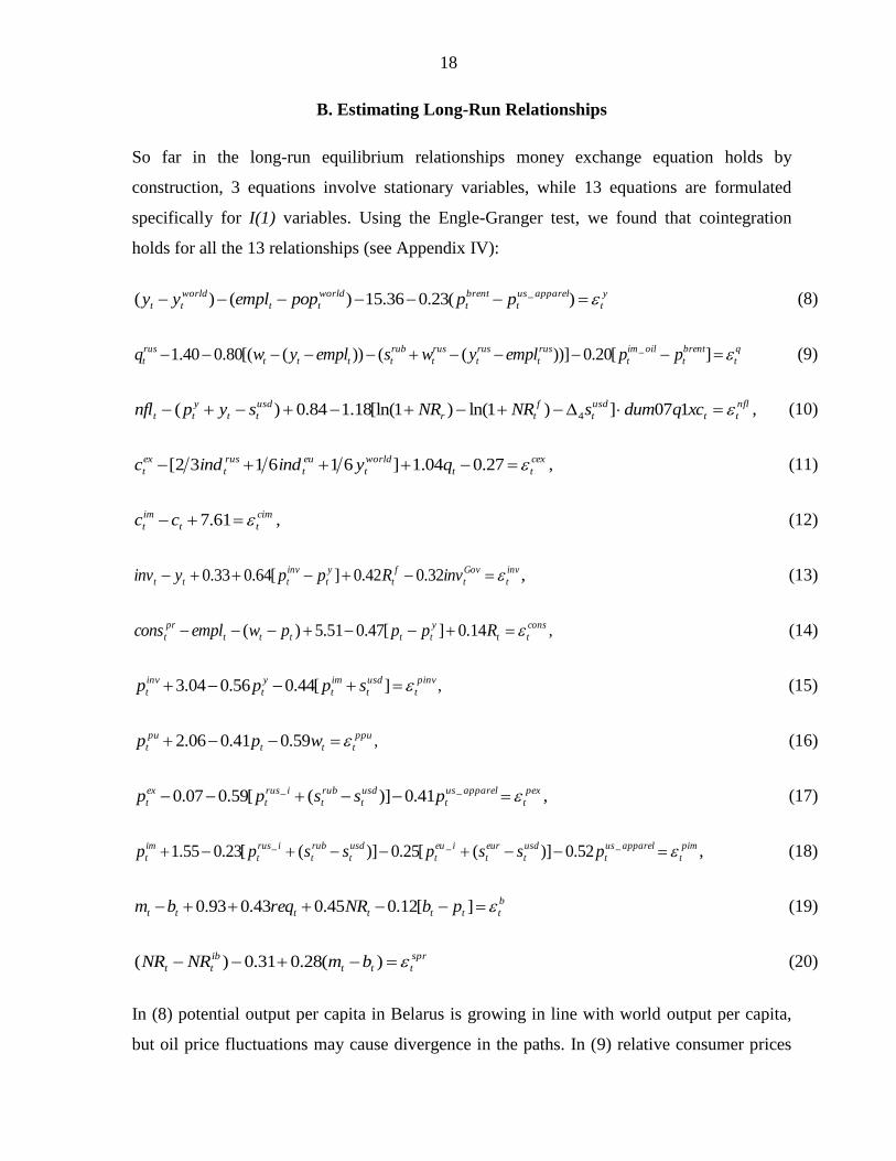
So far in the long-run equilibrium relationships money exchange equation holds by

construction, 3 equations involve stationary variables, while 13 equations are formulated

specifically for I(1) variables. Using the Engle-Granger test, we found that cointegration

holds for all the 13 relationships (see Appendix IV):

y

t

apparelus

t

brent

t

world

tt

world

tt pppopemplyy )(23.036.15)()( _ (8)

q

t

brent

t

oilim

t

rus

t

rus

t

rus

t

rub

tttt

rus

t ppemplywsemplywq ][20.0))](())([(80.040.1 _ (9)

nfl

tt

usd

t

f

tr

usd

tt

y

tt xcqdumsNRNRsypnfl 107])1ln()1[ln(18.184.0)( 4 , (10)

cex

tt

world

t

eu

t

rus

t

ex

t qyindindc 27.004.1]616132[ , (11)

cim

tt

im

t cc 61.7 , (12)

inv

t

Gov

t

f

t

y

t

inv

ttt invRppyinv 32.042.0][64.033.0 , (13)

cons

tt

y

ttttt

pr

t Rpppwemplcons 14.0][47.051.5)( , (14)

pinv

t

usd

t

im

t

y

t

inv

t sppp ][44.056.004.3 , (15)

ppu

ttt

pu

t wpp 59.041.006.2 , (16)

pex

t

apparelus

t

usd

t

rub

t

irus

t

ex

t psspp __ 41.0)]([59.007.0 , (17)

pim

t

apparelus

t

usd

t

eur

t

ieu

t

usd

t

rub

t

irus

t

im

t psspsspp ___ 52.0)]([25.0)]([23.055.1 , (18)

b

ttttttt pbNRreqbm ][12.045.043.093.0 (19)

spr

ttt

ib

tt bmNRNR )(28.031.0)( (20)

In (8) potential output per capita in Belarus is growing in line with world output per capita,

but oil price fluctuations may cause divergence in the paths. In (9) relative consumer prices

19

are driven by relative costs, notably, by unit labour costs and oil prices, which captures the

Harrod-Balassa-Samuelson effect and allows for oil price shocks. In (10) net foreign

liabilities of private sector grow in line with GDP, but investors may take excessive long or

short currency position given UIP deviations. The dummy variable dum07q1xct accounts for

the fact that Belarus was not an active player in the international financial market before

2007, so that interest rate differentials could not have any effect.14 From (17) it follows that

export prices that exclude energy and potash are completely driven by pricing-to-market

principles, so that real exchange rate fluctuations do not affect them (in USD terms), but

rather affect the gap between prices for domestic goods sold in Belarus and abroad. In (11),

demand for export (excl. energy and potash) depends on foreign demand and the real

exchange rate. In (12), demand for non-energy import depends on domestic absorption, while

the real exchange rate effect turned out to be insignificant. Foreign prices completely drive

import prices, as shown in (18). In (13)-(14), demand for investment and private

consumption depends on income levels, their relative prices, and the real interest rates.

However, the foreign-currency real interest rate matters for the former, since foreign

currency loans are widely used to finance investment. Domestic currency dominates

household lending, which makes domestic real interest rate significant in (14). Also, directed

lending has strong impact on investment. In (15) the investment deflator is homogeneous

with respect to GDP deflator and import prices. Similarly, in (16) public consumption

deflator is homogeneous with respect to consumer prices and nominal wages. In the money

supply equation (19), the money multiplier is determined by reserve requirements, nominal

interest rate (which capture both real interest rate and inflation expectations prevailing in the

economy) and the process of economy monetization (as reflected by real monetary base).

Lastly, (20) represents the term structure of interest rates.

C. Estimating Short-Run Relationships

Full results of estimating (1) are in Appendix V. Here we focus on the estimated interest rate

(NRtib

) and reserve money (bt) equations to describe prevailing policy strategy and

instruments.

14

Also, like in real interest rates, the dummy is equal zero during and 1 year after currency crises (2009,

2011q2-2012q3), as we are unable to capture devaluation expectations at that period.

20

We find that the short-term interest rate (NRtib

) responds to both FX interventions (Intyt) and

inflation deviating from the target [∆4pt - πt+]: in (6), χ1,ib < 0 and χ2,ib > 0. The output gap

(εtygap

) is not statistically significant, i.e. χ3,ib = 0. We interpret this as evidence that the NBRB

attempted to pursue a strategy with two objectives – inflation and exchange rate. However, as

discussed in section III.D, interventions were not sterilized and the interest rate was reacting

to interventions-driven changes in domestic liquidity, i.e. the interest rate did not focus on

inflation alone.

The reserve money (bt) is determined by demand for liquidity (εtb), non-sterilized

interventions (Intyt) and money demand (εtv

+ εtygap

). Similar to the impact of FX

interventions on the money market interest rate, χ4,b > 0 and statistically significant indicates

that interventions impacted domestic liquidity conditions. Given that and statistically

insignificant χ2,b and χ3,b, domestic reserve money in (7) is most likely endogenous and hence

not an active policy instrument.

We also find a structural break in SPL dynamics in 2011Q2, but no evidence of breaks in

other equations. Thus, we cannot reject the hypothesis of super exogeneity of SPL with

respect to the remaining equations (Engle et al., 1983): the change in SPL behaviour does not

change the other relationships in the model, so that we can use the model to study impulse

response analysis to permanent SPL shifts.

D. Model Representation to Study Shocks: Ordering of Variables

The covariance matrix of shocks Σ in the reduced form model is not diagonal, i.e. some

shocks are simultaneously correlated. Thus, we need to sequence variables and apply

Choleski decomposition to Σ to identify the model and study responses to structural shocks.

Authorities set targets for some of the variables well in advance. The NBRB always decided

an explicit or implicit objective for BYR/USD exchange rate (stusd

). The 5-year state

programs or annual plans determined SPL (invtGov

) and targets for wages (wt). Therefore, we

assume stusd

, invtGov

or wt do not respond to other variables’ shocks. Additionally, stusd

is

ordered first, i.e. it does not simultaneously respond to invtGov

or wt, but the reverse causality

is possible (e.g., in the event of a currency crisis). Also, we assume invtGov

precedes wt.

21

To sequence the rest we consider two options. First, the policy interest rate (NRtib

),

simultaneously affects demand components (invt, constpr

, constpu

, ctex

, ctim

), prices (ptinv

, pt,

ptpu

, ptex

, ptim

) and monetary aggregates (mt, bt). In such a case, the impulse responses were

anomalous: higher interest rate leads to higher output and inflation, which is a “price

puzzle”.15 Second, the policy rate is ordered after demand components, prices and money.

Impulse responses were adequate in that case and we, therefore, prefer this ordering. Also,

we assume that the policy rate precedes the rate for loans (NRt).

We order NRtib

prior to nflt. In this case, a positive foreign financing shock decreases the

interest rate simultaneously, while positive shock to interest rates induces capital inflow.16

Next, we order the demand components (invt, constpr

, constpu

, ctex

, ctim

), prices (ptinv

, pt, ptpu

,

ptex

, ptim

) and monetary aggregates (mt, bt). Since we consider money as endogenous and

demand driven, rather than a policy instrument, we assume demand or prices simultaneously

affect money aggregates, but money affect macroeconomic indicators only with a lag. We

remain agnostic whether prices simultaneously affect demand components or vice versa and

use the former ordering. However, for robustness we check the ordering of demand

components prior to prices: results are broadly similar in both cases.

As noted in, for example, Garratt et al (2006), when using the Choleski decomposition,

impulse responses differ only with respect to the subset of variables before and after the

shocked variable, but not with respect to ordering within the subsets.17 Thus, for the purpose

of our analysis we use arbitrary sequencing: foreign prices come before domestic in (ptim

, ptex

,

pt, ptinv

, ptpu

), export precedes domestic demand components followed by import in (ctex

,

constpu

, constpr

, invt, ctim

). Also, money precede reserve money (mt, bt), as we assume the

latter is driven by demand for liquidity.

Taking everything together, we obtain the following ordering: stusd

, invtGov

, wt, ptim

, ptex

, pt,

ptinv

, ptpu

, ctex

, constpu

, constpr

, invt, ctim

, mt, bt, NRtib

, NRt, nflt.

15

See, for example, Sims (1992), Eichenbaum (1992).

16 If, in contrast, nflt precedes NRt

ib, then a positive foreign financing shock led to higher money market rate.

This is not consistent with the easing of monetary policy in reaction to capital inflows or decreasing money

market rate, when domestic liquidity increases after the non-sterilized FX interventions. 17

For example, to study the effect of the exchange rate devaluation on demand, the ordering of the exchange

rate prior to demand or after it is important , but not the ordering within the set of demand components.

22

V. IMPULSE RESPONSE ANALYSIS

To examine the features of monetary policy transmission mechanism prevailing in Belarus

during 2001-2014 and some of the long-run properties of the model, we start with impulse

responses to the policy rate and the exchange rate shocks. Then we turn to impulse responses

to wage shocks and shifts in SPL, which are the focal points of our research. For the sake of

brevity, we report the usual demand and supply as well as monetary base shocks in Appendix

VI: the dynamic responses are standard, with demand and monetary base shocks being short-

lived and of limited effect.

A. Monetary Policy Transmission: Policy Rate Shock

The effect of the 1 percentage point policy rate shock on the economy is negligible (Figure

6), which confirms earlier findings of weak interest rate channel in Belarus (Kallaur et al.,

2005; Horvath and Maino, 2006). Given the small effect on demand and output, the interest

rate effect on wages and prices is also limited. The policy rate is remarkably persistent with a

half-life of five years. In the long-run, real variables remain unaffected according to

monetary policy neutrality. Also, stock equilibrium is ensured. The ratio of net foreign

liabilities to GDP gradually returns to its long-run level, in line with the foreign debt

solvency constraint. The money-to-GDP ratio remains at the initial level.

Figure 6: Impulse response to 1pp policy rate shock

23

B. Monetary Policy Transmission: Exchange Rate Shock

The 1 percentage point nominal depreciation (Figure 7) decreases the real exchange rate. This

switches demand to domestically produced goods and fuels export-driven expansion and

reduction in import. Foreign trade improves and offsets initial capital outflow: the NBRB

intervenes in the FX market and accumulates reserves equivalent to about 0.25 percent of GDP

during the second year.18 Output peaks at 0.7 percentage points within a year. Increased

activity leads to higher wages. The latter and higher imported inflation puts upward pressure

on prices, which in three years converge to a new nominal level anchored by the exchange

rate. Monetary policy is passive: the money market interest rate does not initially react to the

shock, and the money stock adjusts to the new price level with a lag. Increasing prices

gradually erase initial competitiveness gains, and reverse the dynamics of output and foreign

trade. Eventually, all the gaps of real variables close, while prices, wages and money are at a

new nominal level anchored by the exchange rate. The long run monetary policy neutrality

and stock equilibrium take place again.

18

Note here and below that the ratios of trade balance, foreign financing and interventions to GDP are provided

in the graphs in per quarter terms. This implies that interventions to GDP per year is the average (rather than the

sum) of quarterly values.

24

Figure 7: Impulse response to 1 percent devaluation shock

C. Wage Shock

In this section, we analyse the consequences of the government’s activist wage policy, which

is one of the focal points of our paper. We consider two kinds of shocks to nominal wages: a

relatively “small” 1 percent shock and a “moderate” 5 percent shock.19 These shocks have

rather different consequences for economic dynamics and the nominal exchange rate anchor.

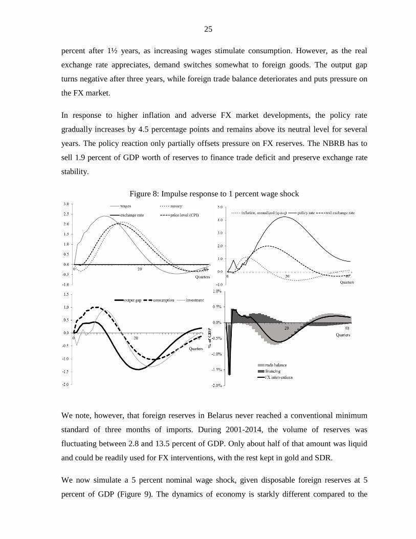
The 1 percentage point nominal wage shock (Figure 8) leads to an immediate foreign finance

outflow of 0.4 percent of annual GDP, which could be attributed to household purchase of

foreign currency. The nominal wage hike induces gradual price increase (with a half-year

lag). In response, wages increase even higher, implying strong real wage persistence as the

Government attempts to fulfil the wage targets. The real wage gap remains positive for

almost three years, while inflation stays above its normal level. The output gap peaks at 0.7

19

Since 2005, nominal wages grew by 2-6.5% per quarter (corrected for seasonal fluctuations). In a number of

quarters nominal wage growth accelerated above 6.5%, in particular: 2005Q4, 2006Q1 and 2008Q1 – about

7.5%, 2010Q2 and 2010Q3 – about 8% and picking up to 12.5% in 2010Q4. Wage growth conformed

hyperinflation in 2011, but remained high in 2012: at 21.5% in 2012Q1 and 11.5% in 2012Q2 and 2012Q3..

These wage spikes provided a rough idea for calibrating nominal wage shocks in our work.

25

percent after 1½ years, as increasing wages stimulate consumption. However, as the real

exchange rate appreciates, demand switches somewhat to foreign goods. The output gap

turns negative after three years, while foreign trade balance deteriorates and puts pressure on

the FX market.

In response to higher inflation and adverse FX market developments, the policy rate

gradually increases by 4.5 percentage points and remains above its neutral level for several

years. The policy reaction only partially offsets pressure on FX reserves. The NBRB has to

sell 1.9 percent of GDP worth of reserves to finance trade deficit and preserve exchange rate

stability.

Figure 8: Impulse response to 1 percent wage shock

We note, however, that foreign reserves in Belarus never reached a conventional minimum

standard of three months of imports. During 2001-2014, the volume of reserves was

fluctuating between 2.8 and 13.5 percent of GDP. Only about half of that amount was liquid

and could be readily used for FX interventions, with the rest kept in gold and SDR.

We now simulate a 5 percent nominal wage shock, given disposable foreign reserves at 5

percent of GDP (Figure 9). The dynamics of economy is starkly different compared to the

26

“small” shock scenario. Increasing domestic prices put pressure on competitiveness and leads

to a mounting current account deficit. Foreign reserves deplete in four years, the currency crisis

follows and the NBRB is forced to devalue to restore the external balance. The 15 percent

devaluation improves competitiveness, stabilizes the FX market and stimulates output. In the

longer-run, wages and prices converge to the new level of the nominal exchange rate.

Figure 9: Impulse response to 5 percent wage shock (Disposable reserves =5 percent of GDP)

D. State Program Lending Shift

Similar to the case of wages we now study shifts in SPL of two magnitudes – 1 and 5

percentage points. Increase in SPL by 1 pp shifts investments upwards and opens positive

output gap. The latter pushes wages and prices up, causing an appreciating real exchange rate

and deteriorating foreign trade. In response to these adverse developments, monetary policy

tightens (interest rates increases), pushing output, prices and wages to the neutral level.

Eventually the permanent increase in SPL shifts demand composition from consumption

towards investments. The market interest rate increases permanently by about 1.5 percentage

points to accompany this shift. Inflation and real wages remain elevated for a number of

years and converge to the long-run levels with significant lags. Along this convergence path,

27

the exchange rate remains appreciated and the foreign trade balance remains negative, which

requires extensive FX interventions (2 percent GDP) to support the peg. In the long-run,

aggregate output returns to its potential level.20

Figure 10: Impulse response to 1 percent SPL shift

Given low FX reserves, it is likely that equilibrium restores via different mechanics if a

larger SPL shift takes place. To illustrate that, we simulate a 5 percent shift, assuming

disposable reserves at 5 percent of GDP (Figure 11). Growing total demand increases imports

and current account deficit. As a result, reserves decrease for nine years to the extent such that

the exchange rate needs to devalue by about 2 percent. Demand rebalances and external

equilibrium restores at a permanently higher level of investment and interest rate, and lower

consumption.

20

We admit that the model does not model any SPL effect on the potential output. In principle, there could be

long-run effects stemming from capital accumulation or changes in total factor productivity. However, studying

these effects requires different type of model and falls beyond the scope of our research.

28

Figure 11: Impulse responses to 5 percent SPL shift (FX reserves = 5 percent of GDP)

VI. POLICY DISCUSSION AND CONCLUSION

We investigated the consequences of two important elements – activist wage policy and state

program lending – for broader macroeconomic stability and sustainability of the monetary

policy strategy prevailing in Belarus during 2001-2014.

First, we showed that a relatively mild positive shock to wages suppresses price

competitiveness and stimulates current account deficits. Highly persistent real wages prolong

the period of imbalances. Ultimately, foreign reserves diminish to an intolerable threshold in

about 4 years and the NBRB has to realign (i.e., devalue) the nominal exchange rate to

facilitate economic adjustment.

Second, similar dynamics are found in response to an increase in SPL. The NBRB sustains

only small shocks, while larger changes lead to devaluation. In the longer run, consumption

decreases permanently to accommodate higher investment. The interest rate for market loans

permanently increases and limits access to non-subsidized domestic denominated credit.

29

Third, a tighter interest rate is sufficient to avoid devaluation only if shocks to wages or SPL

are small. Otherwise, the deteriorating current account exhausts foreign reserves before the

elevated interest rates compresses demand to take economy back to equilibrium.

Although a weak interest rate channel is natural for a developing banking system, there were

other forces at work to render it weak in Belarus. Although imperfect capital mobility

allowed for some monetary autonomy, the efficiency of the interest rate instrument was

limited by the rigid nominal exchange rate. The interest rate differential stimulated foreign

capital flows and perceived stability of the nominal exchange rate suppressing FX risk

perception, which incentivised borrowers to switch from domestic to foreign currency.

More importantly, there were structural reasons for a weak domestic interest rate channel.

Structural weaknesses of the financial system often underlie weak interest rate channel in

low-income and developing countries for various reasons (Mishra et al., 2010, 2012, 2014).

In the specific case of Belarus the major factor behind it was likely to be the SPLs. State-

owned enterprises dominating the economy were subject to government production targets,

and were provided extensive state support, including the SPL. Under such lending banks had

little autonomy in deciding conditions and allocation of loans. The pass-through of the

money market rate to longer-term rates was limited due to inelastic rates for SPL. Further,

the activist wage policy and SPLs were pushing the market interest rates up via two

mechanisms. First, large state-owned banks likely added premia to rates charged on market

(i.e., non-subsidized) loans to offset liquidity and profitability pressures as they financed

subsidized SPL. Second, both quasi-fiscal policies were keeping inflation high, which was

prompting the NBRB and banks to keep the rubel market interest rates high. The elevated

interest rates limited the flow of credit at market rates and the reach of the interest rate

channel.

Overall, government quasi-fiscal objectives contradicted the established monetary policy

strategy: positive increases to wages or SPL undermined the nominal exchange rate anchor.

Monetary policy did not have enough buffers (reserves) and was too limited in its reach via the

interest rate channel to offset the shocks and ensure macroeconomic stability. We can see this

case if the government puts in place its own rigid (due to wage targets) “new nominal anchor”.

30

The activist wage policy dominates monetary policy and the exchange rate adjusts through the

mechanism of a currency crisis to a new nominal level anchored by nominal wages.21

Another way of looking at the issue is the monetary-fiscal strategic game as described in

Nordhaus (1994). The government undertakes (quasi-) fiscal expansion via expanding SPLs

and directing state enterprises to increase wages. The game may potentially end in Nash

equilibrium where the central bank reaches his exchange rate objective (and wins) at a cost of a

high interest rate, while government is not able to reach economic objectives inconsistent with

the long-run equilibrium, and (quasi-) fiscal expansion is not effective despite a high deficit.

In our case, however, the central bank does not have a strong enough interest rate instrument to

win the game. All it largely has is interventions, limited due to small foreign reserves. The

central bank is therefore destined to lose this game with undesired consequences for the

exchange rate and macroeconomic stability.

A number of important conclusions for monetary and broader economic policy follow.

Clearly, there must be only one nominal anchor in the economy, other nominal variables

being endogenously determined. The power to decide the level of the nominal anchor has to

remain with a central bank capable to defend the anchor.

Making the central bank capable involves rethinking the NBRB policy strategy and

approaches to broader economic policy. Since fixed exchange rate regime does not appear

viable in current conditions of low foreign reserves and weak alternative adjustment

mechanisms (incl., due to wage and labour market rigidities), it would be useful for the

NBRB to change its policy focus from the exchange rate to inflation. In fact, the low degree

of international capital mobility in Belarus leaves room for the NBRB to migrate to the

intermediate policy strategy of two objectives and two instruments, with a focus on the

inflation target and a more flexible exchange rate smoothed via fully sterilized interventions

(Ostry et al., 2012). Such a change of regime would require monetary policy to be more

21

Besides, this may have important consequences for inflation expectations. Although fixed exchange rate is

intended to stabilize expectations, rational agents would account for wage targets and allow for devaluations (the

so called “peso problem”). This contributes to the instability of the monetary policy regime via elevated inflation

expectations.

31

forward-looking and decisive in its reaction to shocks. The new regime would allow for

smoother adjustment of external imbalance and lower chances for crisis-like realignments. In

a longer-run, a recurring sense of FX risk being present could help reorienting unhedged

households and corporates to borrowing in domestic currency and, therefore, strengthening

the interest rate channel. However, possibilities of the NBRB to stabilize economy will

depend on consistency of the Government economic policy.

Changes in the monetary policy framework will not ensure broad and lasting macroeconomic

stability as long as quasi-fiscal wage and SPL policies remain active. Discontinuing the wage

policy and allowing wages to adjust according to a usual market mechanism would help on

several fronts: namely, by eliminating the contradiction of anchors, stabilizing expectations

and removing the source of ultimate currency crises. Flexible wages would turn from a

source of imbalances to a shock absorber. Reduction in the SPL would have a similar effect.

Additionally, the extent of redistribution and creating a two-fold economy – with one part

entitled to subsidized loans and the other made to internalize losses via higher inflation and

cost of market loans – would then be duly limited. This would also remove key structural

weaknesses in the banking system and strengthen monetary policy transmission channels.

Lastly, inflation would moderate and give way to a lower long-term level of interest rates,

better access to the domestic currency denominated credit and, again, stronger interest rate

channel. Ultimately, the NBRB would be better placed for conducting independent monetary

policy and stabilizing economy.

It is worth noting that recent changes in macroeconomic policy are in line with our

recommendation. Since 2014, government adopts annual SPL financing plans with the aim to

reduce SPL. In 2015, the NBRB switched to monetary targeting and managed floating

exchange rate. These steps are welcome changes.

32

REFERENCES

Bernanke, B. and I. Mihov (1998): “Measuring monetary policy,” Quarterly Journal of

Economics CXIII, 315-34.

Branson, W. and D. Henderson (1985): “The Specification and Influence of Asset Markets”,

Handbook of International Economics, vol. 2, 749-805.

Eichenbaum, M. (1992): Comments on “Interpreting the Macroeconomic Time Series Facts:

the Effects of Monetary Policy.” European Economic Review, 36(5), 1001-11.

Engle, R., D. Hendry and J.-F. Richard (1983): “Exogeneity”, Econometrica, 51, 277-304.

Flood, R. and P. Garber (1984): “Collapsing Exchange Rate Regimes: Some Linear

Examples”, Journal of International Economics, 17, 1-13.

Garratt, A., K. Lee, M.H. Pesaran and Y. Shin (2006): Global and National

Macroeconometric Modelling: A Long Run Structural Approach, Oxford University

Press, Oxford.

Horvath, B. and R. Maino (2006): “Monetary Transmission Mechanisms in Belarus”, IMF

Working Paper, 06/246.

IMF (2015): Republic of Belarus: Country Report 15/136.

Kallaur, P., V. Komkov and V. Chernookiy (2005): “Monetary Policy Transmission

Mechanism in the Economy of the Republic of Belarus” (in Russian), Belarusian

Economic Journal, 3, 4-15.

Koczan, Z. (2014): “Wage Dynamics in Belarus”, IMF Country Report - Selected Issues,

14/227.

Komkov, V., M. Demidenko and I. Beliatskiy (2008): “Inflationary Consequences of Price

Increase for Imported Resources” (in Russian), Bankovskiy vestnik, 28, 5-11.

Krugman, P. (1979): “A Model of Balance-of-Payments Crises”, Journal of Money, Credit

and Banking, 11, 311-325.

Kruk, D. and K. Haiduk (2013): “The Outcome of Directed Lending in Belarus: Mitigating

Recession or Dampening Long-Run Growth?”, EERC Working Paper, 13/05.

Lucas, R. (1976): “Econometric Policy Evaluation: A Critique”, Carnegie-Rochester

Conference Series on Public Policy, 1, 19-46.

Miksjuk, A. and M. Pranovich (2007): “VECM and Analysis of the Rubel Interbank Credit

Market in Belarus” (in Russian), Bankovskiy vestnik, 34, 19-27.

33

Mishra, P., P.Montiel and A.Spilimbergo (2010): “Monetary Transmission in Low Income

Countries”, IMF Working Paper 10/223.

Mishra, P. and P. Montiel (2012): “How Effective Is Monetary Transmission in Low-Income

Countries? A Survey of the Empirical Evidence”, IMF Working Paper 12/143.

Mishra, P., P. Montiel, P. Pedroni and A.Spilimbergo (2014): “Monetary Policy and Bank

Lending Rates in Low-Income Countries: Heterogeneous Panel Estimates”, Journal of

Development Economics 111, 117-131.

Nordhaus, W. (1994): “Policy Games: Coordination and Independence in Monetary and

Fiscal Policies”, Brookings Papers on Economic Activity, 2, 139-216.

Ostry, J., Ghosh, A. and M. Chamon (2012): “Two Targets, Two Instruments: Monetary and

Exchange Rate Policies in Emerging Market Economies,” IMF Staff Discussion Note,

12/01.

Sims, C., (1992): “Interpreting the Macroeconomic Time Series Facts: the Effects of

Monetary Policy,” European Economic Review, 36(5), 975-1000.

Stock, J.H. and M. W. Watson (2001): “Vector Autoregressions,” Journal of Economic

Perspectives, 15(4) 101–15.

34

APPENDIX I. LONG-RUN EQUILIBRIUM RELATIONSHIPS

We define our long-run relationships by working with equilibrium or arbitrage conditions

that are expected to prevail in the market22. The alternative approach would be to use some

form of utility function, solve the inter-temporal optimization problem for a representative

agent, impose log-linear approximation for the obtained relationships and assume that the

economy is stationary and ergodic in the long run. As noted by Garrett et al. (2006), these

two approaches lead to similar results for the long run properties of the model, but differ for

the short run dynamics.

We assume that technological progress domestically and abroad follow the same long-run

path, though commodities price fluctuations may also prove important given the difference in

economies’ structure. Home per capita output is homogeneous with respect to foreign

output23:

y

tt

com

ttttt ppemplemplyy )()()( *

10

**, (A1)

where yt and yt* are levels of output, emplt and emplt

* are levels of employment, pt

com is

commodities prices, pt* is foreign prices.

Both domestic and foreign prices are set with constant mark-up to nominal marginal costs

(labour, energy and non-energy import costs). Then, relative prices depend on relative costs,

allowing for Harrod-Balassa-Samuelson effect:

q

t

im

t

im

t

en

t

en

t

tttttttt

pppp

emplywsemplywq

])[1(][

))](())([(

*

43

*

4

***

32, (A2)

where qt is real exchange rate, wt and wt* are nominal wages, pt

en and pt

en* are energy import

prices, ptim

and ptim*

are non-energy import prices, st is the nominal exchange rate.

We assume the standard exchange equation holds:

22

Detailed derivation of the theoretical model may be found in the supplementary appendix at:

http://www.jvi.org/about/staff-list/staff-detailview/member/mikhail-pranovich.html

23 From here on, “*” indicate foreign variables and all lower-case variables are in natural logs.

35

v

t

hp

tttt vypm , (A3)

where mt is money stock, vthp

is money velocity trend.

FX market equilibrium is defined by the balance of payments identity:

][])[( t

pr

t

pr

t

en

t

im

t

im

t

ex

t

ex

tt NflFdiTransfTBCPCPInt , (A4)

where Intt is central bank FX interventions vis-à-vis the private sector (net sales of foreign

assets), Ptex

, Ptim

, Ctex

, Ctim

are export and import prices and volumes defining non-

commodities trade balance, TBten

is the commodities trade balance (assumed exogenous),

NFLt is net foreign liabilities of the private sector, Transftpr

and Fditpr

are the remaining

current-account and financial-account operations of the private sector that we assume

exogenous.

Given solvency constraint, one-sided interventions are not sustainable in the long-run:

int0 ttInt . (A5)

Output growth and deviations from the UIP drive equilibrium private net foreign liabilities:

nfl

ttt

f

tttttt sENRNRbbsypnfl ])1ln()1[ln()( 154 , (A6)

where NRt and NRtf are domestic and foreign interest rates, Et is the expectations operator.

Under different circumstances, alternative components of the BOP identity (A4) may prove

important for the FX market. Foreign trade flows played major role in early 20th

century. The

UIP is considered as an equilibrium condition in advanced economies, since capital flows

liberalization in 1960s. In emerging economies like Belarus, capital flows mobility may de

facto be constrained, limiting the importance of the UIP. Thus, we account for both, foreign

trade and financial flows in our model. To treat the trade flows, we add all GDP expenditure

components to the model. In volumes:

][][ __ en

t

menim

t

imen

t

xenex

t

ex

t

dem

t mcxccy (A7)

pub

t

pr

ttt ConsConsInvC (A8)

36

cex

ttt

ex

t qcc 1211

* , (A9)

cim

ttt

im

t qcc 1413 , (A10)

inv

t

Gov

t

f

tt

y

t

inv

ttt invRRppyinv 103210 ][ , (A11)

,])[1()(7654

cons

t

f

tt

y

ttttt

pr

tRRpppwemplcons (A12)

.98

cpu

tt

pu

templcons (A13)

Respective prices:

)]()([)]()([ __

t

M

t

men

t

im

t

im

t

X

t

xen

t

ex

t

expu

t

cpuinv

t

inv

t

consy

t spspspsppppp (A14)

pinv

tt

im

t

y

t

inv

t sppp ])[1( 202019 (A15)

ppu

ttt

pu

t wpp )1( 222221 (A16)

pex

tttt

ex

t sppp ])[1( 16

*

1615 , (A17)

pim

tttt

im

t sppp ])[1( 18

*

1817 , (A18)

where constpu

, invt, xten

, mten

are real public consumption, investment, commodities export

and import, ptpu

, ptinv

, ptX, pt

M are the corresponding deflators, const

pr is real private

consumption, ct is absorption, pty is GDP deflator, pt

* are foreign prices, Rt and Rt

f are real

interest rate in domestic and in foreign currency.

To analyse the central bank tools, we model the money multiplier and the interest rate spread:

b

tttt

ib

ttttt ppbRRreqbm 2928272625 ][ (A19)

spr

ttt

ib

tt bmRR )()( 2423 , (A20)

where reqt is the required reserves ratio.

37

We treat employment (emplt) as exogenous, implicitly assuming that supply of labor is

inelastic and demographic factors, namely, a fraction of the working-age population drives

equilibrium employment.

Variables εX in (A1)-(A20) are the so called long-run reduced-form disturbances, which

represent some linear combinations of long-run structural disturbances (Garrett et al., 2006).24

Variable vthp

is the long-term trend of vt, which we estimate using Hodrick-Prescott filter.

To estimate the domestic output gap we use disturbance εy in (A1) and neglect technology

and capital accumulations disturbances. Then:

)( **

tt

y

t

ygap

ttt yyyy , (A21)

where foreign output gap ( **

tt yy ) is estimated using Hodrick-Prescott filter.

APPENDIX II. DATA DESCRIPTION

Table A1 presents variables, which we use in our model. Endogenous variables include most of

domestic economic variables and policy instruments. A few domestic variables are treated as

exogenous: employment (Emplt, driven by demographic factors not captured in the model),

money velocity trend (Vthp

), required reserve ratio (Reqt, not considered it as an active policy

instrument) and some balance of payments components (TBten

, Xten

, Mten

, Ptim_oil

, Transftpr

,

Fditpr

) largely determined by idiosyncratic shocks rather than economic factors. All foreign

variables are exogenous.

Some additional clarification regarding the endogenous variables is necessary. We exclude

energy products and potash to get foreign trade volumes (Ctex

, Ctim

) and prices (Ptex

, Ptim

). We

consider the former as exogenously determined in the world commodity market (Belarus has

significant stocks of potash and large oil refinery sector: oil, oil products, gas and potash

constitute 1/3 of Belarusian foreign trade in goods). We exclude foreign borrowing that is

directly linked to domestic operations vis-à-vis the Government or the central bank from

private sector foreign liabilities (Nflt) and foreign exchange interventions (Intyt). Such

specific private sector borrowing is not driven by economic factors (i.e., interest rate

24

For example, the reduced form disturbance in (1): εy=ηt+ηkt+μyt+μyt

38

differential). Rather, it de facto represents indirect foreign borrowing of authorities and is

subject to their policy decisions. We approximate real effective exchange rate (Qt) with a

weighted average of bilateral real exchange rates for two major trading partners: Russia and

Eurozone.

Data on directed lending is available only since 2006, however, and of poor quality at least

until 2009. Disbursement of long-term loans at market conditions is rather limited in Belarus,

and directed lending drives most of the changes in their stock. Thus, we use data on all long-

term banking loans (InvtGov

) to approximate directed lending: in interpreting the results we

still refer to this variable as directed lending. Lastly, interest rates NRt, Rt are net of directed

lending rates.

In the production function we use world GDP (Ytworld

) as the foreign output that drives

technology and capital accumulation, world population (Poptworld

) is a proxy for world

employment, and Brent oil prices (Ptbrent

) is the sources of technology divergence (given

large share of oil refinery sector in Belarus). Demand for exports is approximated with a

combination of volumes of Russian industrial production (Indtrus

), EU industrial production

(Indteu

) and world GDP (Ytworld

) with the weights of 2/3, 1/6 and 1/6 respectively. These

weights largely correspond to directions of trade in non-energy and non-potash exports.

Similarly, export and import prices are approximated with Russian and EU industrial prices

(Ptrus_i

, Pteu_i

) and the rest-of-the-world prices for tradable goods (approximated with US

apparel prices Ptus_apparel

). Finally, in equation (2) we use Russian output (Ytrus

), employment

(Empltrus

) and wages (Wtrus

) to capture Harrod-Balassa-Samuelson effect, and imported oil

prices relative to Brent prices (Ptim_oil

/Ptbrent

) to capture energy shocks.

Table A1. Data description1,2

Variable Description

Endogenous variables

Yt GDP, in 2000 prices

Invt Domestic investment, in 2000 prices

Constpr

Household consumption expenditure, in 2000 prices

Constpu

Government consumption expenditure, in 2000 prices

Ct Domestic demand Ct = Invt + Constpr

+ Constpu

, in 2000 prices

Ctex

Non-energy and non-potash exports volume, 2001Q1=1

39

Ctim

Non-energy imports volume, 2001Q1=1

Pty GDP deflator: value of GDP in current prices over Yt

Ptinv

Investments deflator: investment value in current prices over Invt

Pt Consumer price index3, Jan-2001 = 1

Ptpu

Public consumption deflator: public consumption value in current prices over Constpu

Ptex

Prices of non-energy and non-potash exports, US dollar index, 2001Q1=1

Ptim

Prices of non-energy imports, US dollar index, 2001Q1=1

Qtrus

Real exchange rate of Belarusian rubel against Russian rubel (domestic to foreign prices), 2005=1

Qt Real effective exchange rate index (domestic to foreign prices), 2005=1: Qt=Qtrus[Qt

eu_rus]1/3

, where Qt

eu_rus is bilateral real exchange rates of euro against Russian rubel

Stusd

Nominal exchange rate of Belarusian rubel against US dollar, BLR per 1 USD

Steur

Nominal exchange rate of Belarusian rubel against Euro, BLR per 1 EUR

Strub

Nominal exchange rate of Belarusian rubel against Russian rubel, BLR per 1 RUB

Nflt Net foreign debt liabilities of the private sector excl. liabilities related to domestic operations vis-à-vis the Government or the central bank, in USD

NRt Average nominal interest rates on domestic currency banking loans to the economy, % per annum

NRtib Average nominal interest rates for interbank loans in domestic currency, % per annum

Rt Real interest rate on domestic currency banking loans to the economy,4 % per annum:

Rt=(1+NRt)/(1+Pt/Pt-4)-1

Rtib Real interest rate on domestic currency interbank loans,

4 % per annum:

Rtib=(1+NRt

ib)/(1+Pt/Pt-4)-1

Wt Average nominal wages, in rubels

Mt Domestic currency money M2, in rubels

Bt Domestic currency reserve money (monetary base), in rubels

Intyt NBRB’s interventions (net purchase of foreign currency) excl. operations with banks directly linked to banks’ foreign borrowing, % to GDP

InvtGov

Long-term banking loans disbursment to the economy, relative to GDP

Vt Velocity of M2: Vt=PtYt/Mt

Exogenous variables

Emplt Employment, number of people employed

Vthp

Trend of the M2 velocity, estimated using Hodrick-Prescott filter

Reqt Average required reserve ratio: stock of required reserves over the stock of all deposits (in home and foreign prices)

Rtf Real interest rate on foreign denominated banking loans, % per annum: Rt

f=(1+NRt

f)*(1+[st

usd-

st-4usd

])/(1+[pt-pt-4])-1,4

NRtf Average nominal interest rates on foreign denominated banking loans, % per annum

TBten

Energy-and-potash trade balance, in USD

Xten

Volume of energy-and-potash exports calculated using data on volumes and values of oil products, oil and potash exports, weighted average of commodities

Mten

Volume of energy imports, weighted average of energy commodities

40

Ptim_oil

Import oil prices, in USD per ton

Transftpr Net private sector income inflow, including investment income (net of Government percentage

payments on foreign debt), labour income and remittances, in USD

Fditpr

Net FDI inflow excl. privatization, in USD

Ytworld

Trend of world real GDP calculated using linear interpolation of IMF’s annual data, 2000Q4=1

Ytworld_gap

World output gap, estimated using Hodrick-Prescott filter

Ytrus

GDP in Russia, in 2008 prices

Indtrus

Industrial production index in Russia, Jan-2004=1

Indteu

Industrial production index in EU-27, 2001Q1=1

Poptworld

Trend of world population calculated using linear interpolation of UN’s 5-year estimates, number of people

Empltrus

Employment in Russia, number of employed

Wtrus

Average nominal wages in Russia, in RUB

Ptbrent

Brent oil price, USD per barrel

Ptus_apparel

US apparel price index, in USD

Ptrus

Consumer price index in Russia,3 Jan-2001 = 1

Pteu

Consumer price index in EU-27,3 Jan-2001 = 1

Ptim*

Import prices in Russia, 2002Q1=1

Ptrus_i

Producer price index in Russia,3 Dec-2001=1

Pteu_i

Producer price index in EU-27 (domestic market),3 Jan-2001=1

Note: 1 – variables are seasonally adjusted when necessary;

2 – in what follows, lower-case variables

denote natural logarithms of the corresponding upper-case variables; 3

– converted from monthly to quarterly frequency;

4 – we set real interest rates to zero during and 1 year after currency crises (2009,

2011q2-2012q3), as we are unable to capture inflation and devaluation expectations at that period.

APPENDIX III. UNIT ROOT TEST RESULTS

The results of augmented Dickey-Fuller test are provided in Table A2. We use visual

analysis to specify deterministic components in the test (linear trend was included in most

test specifications) and select the lag length based on Schwarz information criterion.

Most of the variables are found to be integrated of order 1 (denoted I(1)) at 5% significance

level. Foreign reserves to GDP ratio (Intyt) and reserve requirements (reqt) are stationary.

World output gap Ytworld_gap

is stationary by definition. There is some ambiguity regarding

nominal exchange rate (strub

), which we assume to be I(1) given that other nominal exchange

rates are I(1). It is not clear whether nominal interest rate NRt is I(1) or I(2) and whether

nominal interest rate NRtib

is I(0) or I(1). We assume the interest rates to be homogeneous

and so to have the same order of integration, I(1).

Test results for world output (ytworld

), Russian output (ytrus

) and Russian wages (wtrus

) are

counter-intuitive, as we do not expect the variables to be I(2). The results change when more

41

lags are introduced in test specification (Table A3). Thus, we assume ytworld

, ytrus

, wtrus

to be

I(1).

Two time series seem to have a structural break. For Belarusian public consumption (constpu

)

there may be a sequence of breaks in 2011-2014, as the authorities were seeking to optimize

the number of public servants. These breaks are difficult to account for, so we truncated the

test period up to III quarter 2011. In this case ADF test indicates constpu

to be stationary.

For the directed lending (invtGov

) there could be a change in trend in 2011, as a new central

bank Governor took office. To account for the structural break we used Perron (1989) unit

root test25 (Table A4). Test results indicate invtGov

be trend stationary at 10% level.

To sum up, we consider all the time series to be I(1), except for Ytworld_gap

, Intyt, reqt, invtGov

and constpu

, which are found to be stationary.

Table A2. ADF test results ADF tests for the levels ADF tests for the first differences

variable test spec† t-statistics p-value variable test spec† t-statistics p-value yt T, 0 0.14 1.00 Δyt C, 0 -7.15 0.00**

invt T, 3 0.33 1.00 Δinvt C, 1 -10.5 0.00**

constpr

T, 0 -2.56 0.30 Δconstpr

C, 0 -9.00 0.00**

constpu

C, 0 -0.90 0.78 Δconstpu

N, 0 -7.36 0.00**

ctex

T, 0 -2.34 0.41 Δctex

C, 0 -6.91 0.00**

ctim

T, 0 -3.22 0.09* Δctim

C, 0 -9.01 0.00**

pty T, 2 -2.73 0.23 Δpt

y C, 2 -3.16 0.03**

ptinv

T, 0 -2.15 0.50 Δptinv

C, 0 -6.75 0.00**

pt T, 1 -2.37 0.39 Δpt C, 1 -3.61 0.01**

ptpu

T, 0 -1.46 0.83 Δptpu

C, 0 -6.53 0.00**

ptex

T, 1 -1.67 0.35 Δptex

C, 1 -5.05 0.00**

ptim

T, 1 -2.56 0.30 Δptim

C, 1 -5.27 0.00**

qtrus

T, 1 -0.89 0.95 Δqtrus

C, 0 -3.58 0.01**

qt T, 1 -1.79 0.70 Δqt C, 0 -4.69 0.00**

stusd

T, 1 -1.73 0.72 Δstusd

C, 0 -4.13 0.00**

steur

T, 1 -2.09 0.54 Δsteur

C, 0 -4.71 0.00**

strub

T, 1 -2.46 0.34 Δstrub

C, 0 -2.81 0.06*

nflt T, 0 -2.68 0.25 Δnflt C, 0 -7.45 0.00**

NRt T, 3 -2.49 0.33 ΔNRt C, 2 -2.75 0.07*

NRt C, 3 -2.69 0.08* ΔNRt N, 2 -2.68 0.01**

NRtib T, 2 -3.24 0.09* ΔNRt

ib C, 1 -7.88 0.00**

NRtib C, 2 -3.62 0.01** ΔNRt

ib N, 1 -7.76 0.00**

wt T, 1 -2.34 0.40 Δwt C, 0 -3.31 0.02**

25

The ADF testing model is extended with dummies allowing for shift in intercept and change in the time trend.

Perron’s critical values are applied to test for unit root.

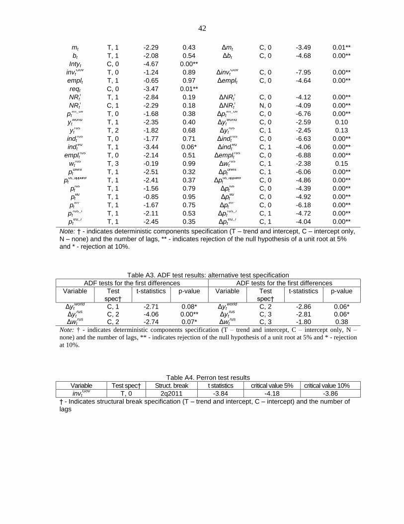
42

mt T, 1 -2.29 0.43 Δmt C, 0 -3.49 0.01**

bt T, 1 -2.08 0.54 Δbt C, 0 -4.68 0.00**

Intyt C, 0 -4.67 0.00**

invtGov

T, 0 -1.24 0.89 ΔinvtGov

C, 0 -7.95 0.00**

emplt T, 1 -0.65 0.97 Δemplt C, 0 -4.64 0.00**

reqt C, 0 -3.47 0.01**

NRtf T, 1 -2.84 0.19 ΔNRt

f C, 0 -4.12 0.00**

NRtf C, 1 -2.29 0.18 ΔNRt

f N, 0 -4.09 0.00**

ptim_oil

T, 0 -1.68 0.38 Δptim_oil

C, 0 -6.76 0.00**

ytworld

T, 1 -2.35 0.40 Δytworld

C, 0 -2.59 0.10

ytrus

T, 2 -1.82 0.68 Δytrus

C, 1 -2.45 0.13

indtrus

T, 0 -1.77 0.71 Δindtrus

C, 0 -6.63 0.00**

indteu

T, 1 -3.44 0.06* Δindteu

C, 1 -4.06 0.00**

empltrus

T, 0 -2.14 0.51 Δempltrus

C, 0 -6.88 0.00**

wtrus

T, 3 -0.19 0.99 Δwtrus

C, 1 -2.38 0.15

ptbrent

T, 1 -2.51 0.32 Δptbrent

C, 1 -6.06 0.00**

ptus_apparel

T, 1 -2.41 0.37 Δptus_apparel

C, 0 -4.86 0.00**

ptrus

T, 1 -1.56 0.79 Δptrus

C, 0 -4.39 0.00**

pteu

T, 1 -0.85 0.95 Δpteu

C, 0 -4.92 0.00**

ptim*

T, 1 -1.67 0.75 Δptim*

C, 0 -6.18 0.00**

ptrus_i

T, 1 -2.11 0.53 Δptrus_i

C, 1 -4.72 0.00**

pteu_i

T, 1 -2.45 0.35 Δpteu_i

C, 1 -4.04 0.00**

Note: † - indicates deterministic components specification (T – trend and intercept, C – intercept only, N – none) and the number of lags, ** - indicates rejection of the null hypothesis of a unit root at 5% and * - rejection at 10%.

Table A3. ADF test results: alternative test specification

ADF tests for the first differences ADF tests for the first differences

Variable Test spec†

t-statistics p-value Variable Test spec†

t-statistics p-value

Δytworld

C, 1 -2.71 0.08* Δytworld

C, 2 -2.86 0.06* Δyt

rus C, 2 -4.06 0.00** Δyt

rus C, 3 -2.81 0.06*

Δwtrus

C, 2 -2.74 0.07* Δwtrus

C, 3 -1.80 0.38

Note: † - indicates deterministic components specification (T – trend and intercept, C – intercept only, N –

none) and the number of lags, ** - indicates rejection of the null hypothesis of a unit root at 5% and * - rejection

at 10%.

Table A4. Perron test results

Variable Test spec† Struct. break t statistics critical value 5% critical value 10%

invtGov

T, 0 2q2011 -3.84 -4.18 -3.86

† - Indicates structural break specification (T – trend and intercept, C – intercept) and the number of lags

43

APPENDIX IV. COINTEGRATION TEST RESULTS

In the model (A4), (A7), (A8), (A14) are identities, (A3) holds by construction, equations

(A5), (A13), (3) are in stationary variables, while (A1), (A2), (A6), (A9)-(A12), (A15)-(A20)

are formulated for I(1). To test the specification of the latter we use Engle-Granger test for

cointegration. The results of the test are reported in Table A5.

In the test, we use MacKinnon p-values, which depend on the number of unrestricted

parameters in the cointegrating relationship (cited first in the second column of Table A5).

The other two parameters in the test specification include deterministic components (selected

based on relationships (A1)-(A20) and (3)) and lag length (selected based on Schwarz

information criterion).

Table A5. Engle-Granger test results

Equation Residual Test spec† t statistics p value Equation Residual Test spec† t statistics p value

(A1) εty 2: C, 0 -3.24 0.08* (A15) εt

pinv 2: C, 0 -5.74 0.00**

(A2) εtq 2: C, 0 -3.23 0.08* (A16) εt

ppu 2: C, 0 -4.08 0.01**

(A6) εtnfl

2: C, 0 -2.54 0.27 (A17) εtpex

2: C, 0 -2.93 0.15 (A9) εt

cex 2: C, 0 -1.88 0.59 (A18) εt

pim 3: C, 1 -4.26 0.02**

(A10) εtcim

1: C, 0 -4.12 0.00** (A19) εtb 4: C, 1 -7.16 0.00**

(A11) εtinv

4: C, 0 -5.85 0.00** (A20) εtspr

2: C, 1 -5.61 0.00** (A12) εt

cons 3: C, 0 -4.41 0.01**

† - Includes the number of stochastic trends cointegration is tested for, deterministic trend specification and lag length, ** - indicates rejection of the null hypothesis of a unit root at 5% and * - rejection at 10%.

Test results confirm cointegration for 8 out of the 13 relationships at 5% significance level,

and for two more relationships at 10%.

Test results for net foreign liabilities, nflt (A6), export volume, ctex

(A9), and export prices,

ptex

(A17) are negative, but cointegration is confirmed when alternative test specification is

used by including extra lag or truncating last quarters of the test period (Table A6).

Table A6. Results of Engle-Granger test: alternative specification

Equation Residual Change in model specification Test spec† t statistics p value

(6) εtnfl

Exclude 2014q2-2014q4 2: C, 1 -3.22 0.08*

(9) εtcex

Exclude 2014q3-2014q4 2: C, 0 -3.21 0.09*

(17) εtpex

Add extra lag 2: C, 1 -3.33 0.07*

† - Includes the number of stochastic trends cointegration is tested for, deterministic trend specification and lag length, ** - indicates rejection of the null hypothesis of a unit root at 5% and * - rejection at 10%.

Overall, we conclude that cointegration holds for all the 13 relationships.

44

APPENDIX V. ESTIMATED REDUCED FORM MODEL

As a first step, we estimate dynamic equations in (1) separately as discussed in section III.E.

In the final specification statistical tests (correlogram and serial correlation LM test) show no

evidence of residual autocorrelation at 5% significance level. Except for the exchange rate

and money stock equations, residuals were found to be homoscedastic (Breusch-Pagan-

Godfrey test). In most cases normality of residuals was not rejected.

Next, we stack equations in a system and estimate it simultaneously using Seemingly

Unrelated Regression method:

][51.0][45.0032.053.0 22111

y

t

inv

t

y

t

inv

t

inv

tt ppppinv (A22)

t

cons

tt

pr

t

pr

t qqdumwconscons 411_21109.035.024.033.0015.0 111 (A23)

tt

pu

t

pu

t xqdumxqdumconscons 31101.021301.017.265.0 1 , (A24)

)105404(07.040825.030.0019.0 1 ttt

cex

t

ex

t qdumqdumqdumc (A25)

]109408[13.0)105404(28.026.0027.0 1 tttt

cim

t

im

t qdumqdumqdumqdumc (A26)

111 11.020.066.0048.0 t

inv

t

pinv

t

inv

t invp (A27)

111

11

_

111

07.007.041404.006.096.0

08.012.003.013.076.0411_21114.0006.0

t

ex

tt

inv

t

rus

t

y

t

q

t

oilim

t

usd

tttt

wcqdumpp

pspqqdump (A28)

pu

tt

ppu

tt

pu

t ppwp 1111 23.065.0020.039.037.0 (A29)

001.035.0)]([66.0 1

_

pex

t

usd

t

rub

t

irus

t

ex

t sspp (A30)

004.0_31.023.0)]([19.0)]([35.0 11

__

im

t

im

t

usd

t

eur

t

ieu

t

usd

t

rub

t

irus

t

im

t pgappsspsspp (A31)

tttt

usd

t qqdumtxqdumqqdumcriss 403_101008.031304.0411_21130.063.1 , (A32)

nfl

ttnfl 123.0048.0 (A33)

sprd

t

ib

tt

ib

tt NRNRNRNR 122 56.0)(20.0002.0][ (A34)

]312_211409_1091)[(58.029.028.0

70.024.0411_21119.038.0030.0

11432

131

tttt

inv

tt

t

ib

ttt

ib

t

qqdumqqdumppb

NRNRqqdumIntyNR

(A35)

45

ex

t

ex

ttttt

q

tt ccwwppw 2121311 11.017.046.023.038.055.0008.010.0 (A36)

][33.0041.054.0 111

ygap

t

v

ttt mm (A37)

][20.022.032.060.0057.032.0 1111

ygap

t

v

ttt

b

ttt Intyreqbb (A38)

Gov

ittt

Gov

t invxqdumtxqdumtinv 55.0211041.021137.1030.075.1 (A39)

According to estimated relationship (A32), during the currency crises the size of devaluation

of the nominal BYR/USD exchange rate was proportional to real exchange rate misalignment

with the coefficient 1.63. Komkov et al. (2008) estimate the full share of import costs (direct

and indirect) in the consumption basket in Belarus at 0.39. Then, nominal devaluation of

1.63% would produce the 1st round effect on inflation equal 0.64% and corresponds to 1%

real devaluation. Therefore, if all other costs are fixed, this nominal devaluation in this

proportion to the misalignment is just enough to ensure real exchange rate adjustment.

According to (A37), money supply (mt) is determined by demand for money captured by the

money velocity gap (εtv) plus the output gap (εt

ygap), which is consistent with p-star model.

Thus, money stock adjusts to real money demand deviation from its long-term trend captured

by velocity trend and potential (rather than actual) output level.

Price (pt) and wage (wt) dynamics is persistent and reacts slowly to the real exchange rate

misalignment (εtq). So, given the rigid nominal exchange rate, the deviations of real exchange

rate from equilibrium are likely to be persistent as well. Inflation reacts to output gap (εty),

but not to the money velocity gap (εtv), so there are no inflationary pressures stemming from

money demand deviations. Within this setting, wages would be positively reacting to output

fluctuations as captured in (9), while inflation would rather be reacting to potential output, as

disinflationary pressure from short-run productivity gains in (9) would be just compensated

with inflationary pressure from output gap (8).

46

APPENDIX VI. IMPULSE RESPONSES TO DEMAND, INFLATION AND MONETARY

BASE SHOCKS

A. Monetary Base Shock

The effect of 1 percent monetary base shock on the economy is negligible with no effect on

output or prices. This confirms our earlier finding that monetary base was driven

endogenously by demand for liquidity, rather than used as an active policy instrument (Figure

A1).

There is some small and short-lived effect in the financial market, however. Monetary

expansion is associated with limited capital outflow, which could be due to credit currency

substitution as more credits can be provided in domestic currency and, hence, less foreign

financing is needed. Policy rate reacts with immediate tightening, which brings liquidity down

and reverts foreign financing, so that the equilibrium is largely restored within a year.

Figure A1. Impulse response to 1 percent monetary base shock

47

B. Domestic Demand Shock

The effect of 1 percentage point domestic demand shock on the economy is limited in scope

and short-lived in time (Figure A2). Increase in demand is satisfied with supply of domestic

goods and imports. Thus, output increases by 0.6 percent within one quarter, whereas foreign

trade balance deteriorates by 0.4 percent of GDP. In response, the NBRB lets the money

market rate to increase to defend the peg, although the scope of the reaction is too small to

prevent the loss of foreign reserves.

Wages and prices almost do not react and the demand shock fades quickly, so the economy

largely returns to the equilibrium in two years. The output gap is closed by the second

quarter, while it takes one more year to eliminate the trade deficit.

Figure A2. Impulse response domestic demand shock (1 percent investment shock)

48

C. Inflation Shock

Unlike the demand shock, the inflation shock of 1 percent has a significant impact on economy

(Figure A3).

Increase in price level is accompanied by negative output gap. The recession is partly due to a

fall of domestic demand, but mostly is driven by a substitution effect, as immediate real

exchange rate appreciation shifts demand towards foreign goods with ensuing foreign trade

balance deterioration.

In response to inflationary pressures and losses of foreign reserves, the NBRB lets the money

market rate to increase, albeit with some delay: after an immediate decline interest rates

increase by 4 percentage points.

Higher interest rate is not enough to offset pressures on the FX reserves: the NBRB

intervenes for about 2½ years (net sell of foreign assets worth 1.9 percent GDP) to defend the

exchange rate peg. Money supply is tightened as well, implying money stock decline in real

terms. Loss of price competitiveness combined with tighter money induces a prolonged

recession with the output gap hitting negative 1.5 percent at its trough. This also puts

pressure on real wages.

Eventually, all these developments – the negative output gap, decline in real wages and

tighter money – make inflationary pressures to reverse by the end of the first year. Prices

gradually converge to their long-run level anchored by the nominal exchange rate. The

economy largely returns to equilibrium within five years.

Figure A3. Impulse response to 1 percent inflation shock

49