The g-theorem and quantuminformation theory

Horacio Casini, Ignacio Salazar Landea, Gonzalo Torroba

Centro Atomico Bariloche and CONICET

S.C. de Bariloche, Rıo Negro, R8402AGP, Argentina

Abstract

We study boundary renormalization group flows between boundary confor-mal field theories in 1 + 1 dimensions using methods of quantum informationtheory. We define an entropic g-function for theories with impurities in termsof the relative entanglement entropy, and we prove that this g-function de-creases along boundary renormalization group flows. This entropic g-theoremis valid at zero temperature, and is independent from the g-theorem basedon the thermal partition function. We also discuss the mutual information inboundary RG flows, and how it encodes the correlations between the impurityand bulk degrees of freedom. Our results provide a quantum-information un-derstanding of (boundary) RG flow as increase of distinguishability betweenthe UV fixed point and the theory along the RG flow.

arX

iv:1

607.

0039

0v2

[he

p-th

] 1

0 A

ug 2

016

Contents

1 Introduction 1

2 The entropic g-theorem from relative entropy 32.1 Boundary RG flows . . . . . . . . . . . . . . . . . . . . . . . . . . . . 32.2 Boundary entropy from relative entropy . . . . . . . . . . . . . . . . . 52.3 Relative entropy for states on the real line . . . . . . . . . . . . . . . 62.4 Proof of the entropic g-theorem . . . . . . . . . . . . . . . . . . . . . 8

3 Mutual information in quantum impurity systems 113.1 Mutual information and correlations . . . . . . . . . . . . . . . . . . 123.2 Impurity valence bond model . . . . . . . . . . . . . . . . . . . . . . 143.3 General analysis . . . . . . . . . . . . . . . . . . . . . . . . . . . . . . 16

4 A free Kondo model 184.1 The model . . . . . . . . . . . . . . . . . . . . . . . . . . . . . . . . . 184.2 Lattice version . . . . . . . . . . . . . . . . . . . . . . . . . . . . . . 204.3 Thermal entropy . . . . . . . . . . . . . . . . . . . . . . . . . . . . . 23

5 Quantum entanglement in the free Kondo model 255.1 Modular Hamiltonian for spatial intervals . . . . . . . . . . . . . . . . 255.2 Kondo model on the null line . . . . . . . . . . . . . . . . . . . . . . 275.3 Mutual information in the free Kondo model . . . . . . . . . . . . . . 32

6 Conclusions and future directions 34

A Nonrelativistic Kondo model 35

B Fermion boundary conditions 35

C Calculation of the modular Hamiltonian 37

Bibliography 37

1 Introduction

Quantum impurities and defects play an important role in different areas of theoret-ical physics, including condensed matter physics, gauge theories, and string theory.

1

In order to understand the possible quantum field theories with defects and their dy-namics, a key step is to classify boundary conditions that preserve some conformalinvariance in bulk conformal field theories (CFTs), together with the renormalizationgroup flows between different boundary conditions.

The best understood situation arises in two-dimensional CFTs with conformalboundaries, which led to the development of boundary CFT (BCFT). This case isespecially interesting, because it arises from spherically symmetric magnetic impuri-ties in metals (as in the famous Kondo problem [1]) and also describes D-branes instring theory [2]. In a 2d CFT, Cardy found that a conformal boundary correspondsto a boundary state [3]. Affleck and Ludwig defined a g-function in terms of thedifference between the thermal entropy with and without impurity, and used the for-malism of boundary states to compute it [4]. The boundary entropy plays the role ofa ground-state degeneracy associated to the impurity, and these authors conjecturedthat g decreases under renormalization. A key result in this direction is the proof ofFriedan and Konechny that establishes that g indeed decreases monotonically alongboundary RG flows [5].

A crucial property of the boundary entropy is that its value at a fixed point is infact (part of) an entanglement entropy, as shown in [6]. However, this equivalenceis not valid away from fixed points, as it uses the conformal map between the planeand the cylinder in two dimensions. This raises the important question of whetherthere exists an “entropic g-function” that decreases monotonically along boundaryRG flows, and whose fixed point values agree with the boundary entropy. Anotherquestion is if g can be defined directly in terms of an entropy. The conformal mapof [6] identifies g with a specific constant term in the entanglement entropy, aftersubtracting the logarithmically divergent area term. This subtraction obscures apossible monotonous behavior.

The goal of this work is to prove an entropic g-theorem, namely that there exists ag-function that decreases monotonically under boundary renormalization, and whosefixed point values agree with g for BCFTs.1 We will accomplish this by identifying gwith a relative entropy; this is our main result and is presented in §2. In the remain-der of the paper we initiate a broader program of using techniques from quantuminformation theory to study boundary RG flows. Specifically, in §3 we focus on themutual information and how it measures correlations between the impurity and bulkdegrees of freedom. In order to illustrate our general results, we introduce in §4 anew relativistic Kondo model, which has the nice feature of being Gaussian and yet

1We would like to mention the previous related work [7], where the authors attempted to provethe g-theorem using strong subadditivity. The holographic version of the theorem was establishedin [8].

2

it leads to a nontrivial boundary RG flow. Various aspects of quantum entanglementfor this theory are analyzed in §5.

2 The entropic g-theorem from relative entropy

In this section we will study boundary RG flows using the relative entropy. Therelative entropy provides a measure of statistical distance between the states of thesystem with different boundary conditions, and we will see that it is closely relatedto boundary entropy. Monotonicity of the relative entropy will be used to prove theg-theorem.

After reviewing boundary RG flows in §2.1, in §2.2 we explain the connectionbetween relative and boundary entropy. The relative entropy compares two densitymatrices: one corresponds to some arbitrary reference state (which in our case willbe related to UV BCFT) and the other one is the density matrix for the system withrelevant boundary flow. The simplest possiblity is to use reduced density matricesfor intervals on the real line. We explore this in §2.3, finding that the monotonicityproperties of the relative entropy do not allow to prove a g-theorem. The reason isthat the relative entropy distinguishes the different states too much, and this masksthe decrease of g under the RG.

This suggests the correct path towards the g-theorem: vary the states in orderto minimize the contribution from the modular Hamiltonian, while keeping fixed theentanglement entropy. This analysis is presented in §2.4. We show that by workingwith states on the null boundary of the causal domain, the contribution from themodular Hamiltonian becomes a constant, and hence the impurity entropy is givenexplicitly as (minus) a relative entropy. We then use this result to prove the entropicg-theorem.

2.1 Boundary RG flows

Let us begin by briefly reviewing the class of RG flows that are studied in this work.The starting point is a CFT defined on x1 > 0 with a boundary at x1 = 0 whichpreserves half of the conformal symmetries – a BCFT. This requires

− iT01(x1 = 0) = T (x1 = 0)− T (x1 = 0) = 0 . (2.1)

A particular case is a CFT with a defect at x1 = 0, which can be folded into a BCFTon x1 ≥ 0.2

2The reverse, unfolding a BCFT into a theory defined on the full line, is not possible in general.We thank E. Witten for pointing this out to us.

3

In general the boundary may support localized degrees of freedom that will becoupled to the fields in the bulk theory. The UV theory, denoted by BCFTUV , isthen perturbed by a set of relevant local operators at the boundary,

S = SBCFTUV+

∫dx0 λiφi(x0) . (2.2)

This perturbation can combine operators from the bulk (evaluated at x1 = 0) and/orquantum-mechanical degrees of freedom from the impurity. The perturbation triggersa boundary RG flow; we assume that the flow ends at another boundary CFT,denoted by BCFTIR.

The boundary perturbation preserves time-translation invariance and is local.In this way, bulk locality is preserved and operators at spatially separated pointscommute. This is needed for using the monotonicity of the relative entropy below.

The boundary entropy log g is defined as the term in the thermal entropy that isindependent of the size of the system [4],

S =cπ

3

L

β+ log g , (2.3)

where L is the size and β the inverse temperature. At fixed points, log g can becomputed as the overlap between the boundary state that implements the conformalboundary condition and the vacuum [3]. For a boundary RG flow, Affleck and Ludwigconjectured that

log gUV > log gIR . (2.4)

Friedan and Konechny [5] proved nonperturbatively that the boundary entropy de-creases monotonically along the RG flow,

µ∂ log g

∂µ≤ 0 , (2.5)

where µ is the RG parameter. It also decreases with temperature, since g = g(βµ)on dimensional grounds.

At a fixed point, the thermal entropy can be mapped to an entanglement entropyby a conformal transformation –see e.g. [6]. Concretely, The ground state entangle-ment entropy of an interval x1 ∈ [0, r), with one end point attached to the boundary,is given by

S(r) =c

6log

r

ε+ c0 + log g , (2.6)

where ε is a UV cutoff, and c0 is a constant contribution from the bulk that isindependent of the boundary condition.

4

Therefore, log gUV > log gIR for the constant term on the entanglement entropyof this interval. However, away from fixed points the entanglement entropy cannotbe mapped to a thermal entropy, and it is not known whether log g(r) defined in(2.6) decreases monotonically. We will prove that this is indeed the case.

2.2 Boundary entropy from relative entropy

The relative entropy between two density matrices ρ0 and ρ1 of a quantum systemis defined as

Srel(ρ1|ρ0) = tr(ρ1 log ρ1)− tr(ρ1 log ρ0) . (2.7)

In terms of the modular Hamiltonian for ρ0, ρ0 = e−H/tr(e−H), it can be written as

Srel(ρ1|ρ0) = ∆〈H〉 −∆S , (2.8)

where ∆〈H〉 = tr ((ρ1 − ρ0)H), and ∆S = S(ρ1) − S(ρ0) is the difference betweenthe entanglement entropies of the density matrices.

Let us recall some basic features of the relative entropy.3 For our purpose, themost relevant property of the relative entropy is that (for a fixed state) it cannotincrease when we restrict to a subsystem. In QFT the reduced density matrix ρV isassociated to a region V and is obtained by tracing over the degrees of freedom in thecomplement V . In this case, the relative entropy increases when we increase the sizeof the region. Some simple properties of the relative entropy are that Srel(ρ1|ρ0) = 0when the states are the same, and Srel(ρ1|ρ0) =∞ if ρ0 is pure and ρ1 6= ρ0.

For the boundary RG flows of §2.1, the reduced density matrix associated toan interval x1 ∈ [0, r) is obtained by tracing over the complement, and defines ag-function

S(r) =c

6log

r

ε+ c0 + log g(r) . (2.9)

This boundary entropy interpolates between log gUV for r � Λ−1 and log gIR forr � Λ−1. Here Λ is the mass scale that characterizes the boundary RG flow. Wewant to show

g′(r) ≤ 0 , (2.10)

and this would imply the entropic version of the g-theorem. Note that even if thetheorem gives a monotonicity g(0) ≥ g(∞) between fixed points, and coincides in thisrespect with the result [5], the interpolating function differs from their interpolatingfunction. Indeed, as emphasized before, the boundary contribution in the thermal

3We refer the reader to [9] for more details.

5

entropy does not map simply into the boundary contribution to the entanglemententropy when the theory is not conformal.

Let ρ be the reduced density matrix on the spatial interval [0, r). We want tocompare ρ with some appropriately chosen reference state ρ0 in terms of the relativeentropy. Since the boundary RG flow starts from a BCFT in the UV, we choose thereduced density matrix ρ0 to be that of BCFTUV . A crucial property that motivatesthis choice is that the modular Hamiltonian H for an interval including the origin inhalf space with a conformal boundary condition is local in the stress tensor, and hasthe same form as that of a CFT in an interval. This can be shown by a conformalmapping to a cylinder [6, 10]; see [11] for a recent discussion.4

Making this choice obtains

Srel(ρ|ρ0) = − logg(r)

g(0)+ tr ((ρ− ρ0)HBCFT ) . (2.11)

The first term comes from the difference in entanglement entropies between thetheory with boundary RG flow (ρ) and the UV fixed point ρ0; from (2.9) this givesprecisely the change in boundary entropy. This gives the relation between the bound-ary entropy and relative entropy, and has the right sign to yield g′(r) < 0 since Srelincreases with r. The second term, however, could be an important obstruction to ag-theorem. It comes from the difference in expectation values of the modular Hamil-tonian between the states with and without the relevant boundary perturbation.The rest of the section is devoted to analyzing this contribution. For the simplestsetup of states defined on the real line, we will find that this term increases with r,masking the monotonicity of g. We will then improve our setup, showing how thisterm can be made to vanish by defining states on null lines.

2.3 Relative entropy for states on the real line

We have to understand the contribution of the modular Hamiltonian to (2.11). Thesimplest possibility is to work with states defined on the real x1 line. In this case, themodular Hamiltonian for a CFT in half-space with a conformal boundary conditionat x1 = 0 is

HBCFT (r) = 2π

∫ r

0

dx1r2 − x2

1

2rT00(x1) . (2.12)

This is the generator of a one parameter group of conformal symmetries that mapthe x1 = 0 line in itself and keeps the end point of the interval x1 = r, t = 0, fixed.

4We thank J. Cardy for explanations on this point.

6

These global symmetries of the CFT continue to be symmetries of the CFT withconformal boundary conditions.

It is important that even in presence of a relevant perturbation on the boundarywe must have 〈T00〉 = 0 outside the x1 = 0 line. This follows from tracelessness,conservation, and translation invariance in the time direction, that give

〈T00〉 − 〈T11〉 = 0 ,

∂0〈T00〉 − ∂1〈T10〉 = −∂1〈T10〉 = 0 , (2.13)

∂0〈T01〉 − ∂1〈T11〉 = −∂1〈T11〉 = 0 .

Hence 〈Tµν〉 is constant outside the boundary and has to vanish.Then 〈T00〉 does not contribute to HBCFT outside the boundary. If this is the

whole contribution to ∆〈HBCFT 〉 we would have from (2.11) that the monotonicityof the relative entropy implies the entropic g-theorem. In particular, −g(r) wouldbe given by the relative entropy between states with and without the boundaryperturbations.

There is still an important aspect to understand: there might be a contribution to〈T00〉 localized at the boundary. On dimensional grounds, we expect for the variationof the expectation values with and without the relevant perturbation

∆〈T00〉 = λ2ε1−2∆ δ(x1) + . . . (2.14)

where λ is the relevant boundary coupling in (2.2) with scaling dimension [λ] =1−∆ > 0, and ε is a distance cutoff. In other words, the boundary operator φ thatdeforms the theory in (2.2) has dimension ∆. Here we have done a perturbativeexpansion for small λ, so that ρ and ρ0 are very close to each other; the first pertur-bative contribution is generically of order λ2. By a similar power-counting argument,more singular contact terms (proportional to λ2ε2−2∆δ′(x1) for example) would van-ish in the continuum limit ε → 0. From (2.12) it is clear that any such localizedcontribution to 〈T00〉 will produce a contribution to ∆〈HBCFT 〉 which is increasinglinearly with r, spoiling a proof of the g-theorem. In the free Kondo model of §4 wewill see that this is indeed the case.

This linear dependence in r implies that the relative entropy distinguishes toomuch the states with and without the impurity on the real line. It is clear that inorder to be able to use the relative entropy to capture the RG flow of g(r) we needto choose states that minimize ∆〈HBCFT 〉. This is the problem to which we turnnext.

7

2.4 Proof of the entropic g-theorem

In order to use the monotonicity of the relative entropy to prove the g-theorem, weneed to minimize the contribution from the modular Hamiltonian. The basic idea isthat in a unitary theory the entanglement entropy is the same on any spatial surfacethat has the same causal domain of dependence. This evident is in the Heisenbergrepresentation, where the state is fixed and local operators depend on spacetime.Local operators written in a given Cauchy surface can in principle be written inany other Cauchy surface using causal equations of motion. Then, the full operatoralgebra written in any Cauchy surface will be the same, and as the state is fixed, theentropy will remain invariant.

The relative entropy for two states in a fixed theory is also independent of Cauchysurface. However, in the present case, as the vacuum states of the theory with orwithout relevant boundary perturbation have different evolution operators, choosinga different surface corresponds to changing the states by different unitary operatorsin each case. In the Heisenberg representation of the BCFT the conformal vacuumwill not change, but the fundamental state of the theory with the relevant pertur-bation will evolve with an additional insertion placed on x1 = 0. As a consequence∆〈HBCFT 〉 will now depend on the choice of surface. Therefore, we need to varythe Cauchy surface until we eliminate the large increasing ∆〈HBCFT 〉 term in therelative entropy.

This approach is illustrated in Figure 1. We want to determine the entanglemententropy S(r) for a spatial interval x1 ∈ [0, r). This interval defines a causal domainof dependence D, and because of unitarity S(r) is the same for any other Cauchysurface with the same D. This applies for both states, since evolution is unitaryinside D independently of the local term in the Hamiltonian at x1 = 0. Hence, ∆Sis independent of the chosen surface Σ.

We want to make ρ as similar as possible to ρ0 in order to minimize the contribu-tion ∆〈HBCFT 〉. The modular Hamiltonian of the BCFT vacuum is proportional tothe generator of conformal transformations that keep the interval fixed. Using theHeisenberg representation corresponding to the BCFT evolution, it can be writtenon any Cauchy surface Σ as a flux of a conserved current

HBCFT =

∫Σ

ds ηµTµνξν , (2.15)

where η is the unit vector normal to the surface and

ξµ ≡ 2π

2r(r2 − (x0)2 − (x1)2 , −2x0x1) . (2.16)

8

Figure 1: Different Cauchy surfaces Σ with the same causal domain of dependence D givethe same entanglement entropy S(r).

We stress again the important point that this current is generally not conserved inthe theory with boundary RG flow, leading to changes in the expectation values ofthe modular Hamiltonian for different surfaces.

Since the expectation values of the stress tensor vanish everywhere except atthe impurity we need to choose a surface where the coefficient of Tµν in the modularHamiltonian vanishes on the line x1 = 0. We accomplish this by working with a stateon the null boundary of the causal development; see Figure 1. In null coordinatesx± = x0 ± x1 this writes

HBCFT = 2π

∫ r

−rdx+ r2 − x+ 2

2rT++(x+) . (2.17)

By locality, the defect at x+ = x− = −r can contribute a contact term of the form

〈T++〉 ∼ δ(x+ + r) (2.18)

and similarly for the T−− component. This effect gives a vanishing contributionin (2.17). This should be contrasted with the situation on the real line, where adelta function 〈T00〉 ∼ δ(x1) already contributes a linear term in r to the modularHamiltonian (2.12).

9

We conclude that, by working with a state on the null segment, the contributionfrom ∆〈H〉 vanishes

Srel(ρ|ρ0) = − logg(r)

g(0). (2.19)

The change in the boundary entropy is then identified as a relative entropy. Notethat with the relative entropy we can measure changes in the boundary entropy, andnot the boundary entropy itself.

In physical terms, the reason that relative entropy is much smaller in the nullsurface than in the spatial one is that in this last case we are placing the impurityat the origin of the interval where the vacuum of the BCFT has an effective lowtemperature ∼ r−1 as can be read off from the coefficient of T00 in (2.12). As aresult the two states are highly distinguishable, having a large relative entropy. Incontrast, the extreme point of the null Cauchy surface (corresponding to x+ = −r)is a point of an effective high temperature, as seen from the fact that the coefficientsof T++ vanish there in (2.17). Hence distinguishability is strongly reduced, and willbe driven by the change of correlations outside the impurity, which will be reflectedin the change of entanglement entropies.

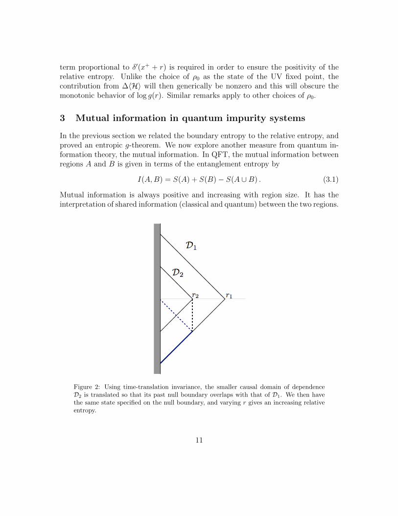
Finally, in order to use the monotonicity of the relative entropy, we need to vary rbut using the same states defined on the null line. This is implemented as explainedin Figure 2. The monotonicity of the relative entropy gives

g′(r) < 0 . (2.20)

This completes our proof of the entropic g-theorem. The relative entropy defines amonotonic g-function, and the total change between the UV and IR boundary CFTsis

Srel(∞)− Srel(0) = log(gUV /gIR) > 0 . (2.21)

This formula is independent of contact terms and establishes a universal relationbetween the change in relative entropy and the total running of the boundary entropy.

In this proof of the g-theorem we have compared the density matrix ρ along theRG flow to the state ρ0 of the UV fixed point. This was used, in particular, toconstrain the form of the contact term divergences in (2.18). While in our contextthis is the most natural choice for ρ0, one may wonder what happens if ρ0 is someother reference state. One possibility along these lines is to use the IR BCFT as thereference. For large enough r, ρ approaches ρ0 on the null line, and the contributionsto ∆〈Tµν〉 are determined by the leading irrelevant operator that controls the flowtowards the IR fixed point. This flow does not have a well-defined UV limit, andhence other divergences besides (2.18) are allowed. In particular, at least a contact

10

term proportional to δ′(x+ + r) is required in order to ensure the positivity of therelative entropy. Unlike the choice of ρ0 as the state of the UV fixed point, thecontribution from ∆〈H〉 will then generically be nonzero and this will obscure themonotonic behavior of log g(r). Similar remarks apply to other choices of ρ0.

3 Mutual information in quantum impurity systems

In the previous section we related the boundary entropy to the relative entropy, andproved an entropic g-theorem. We now explore another measure from quantum in-formation theory, the mutual information. In QFT, the mutual information betweenregions A and B is given in terms of the entanglement entropy by

I(A,B) = S(A) + S(B)− S(A ∪B) . (3.1)

Mutual information is always positive and increasing with region size. It has theinterpretation of shared information (classical and quantum) between the two regions.

Figure 2: Using time-translation invariance, the smaller causal domain of dependenceD2 is translated so that its past null boundary overlaps with that of D1. We then havethe same state specified on the null boundary, and varying r gives an increasing relativeentropy.

11

There are two important motivations for considering the mutual information inthe context of quantum impurity systems. The first motivation is that it providesa measure of the correlations in the system. In more detail, it is a universal upperbound on correlations [12]

I(A,B) ≥ (〈OAOB〉 − 〈OA〉〈OB〉)2

2 ‖OA‖2 ‖OB‖2 (3.2)

for bounded operators OA and OB that act on A and B respectively. The secondreason is the connection with the boundary entropy log g.

Our proposal is to study the dynamics of quantum impurity systems in terms ofthe mutual information between the impurity (subsystem A above) and an intervalof size r in the bulk (subsystem B). We first discuss in §3.1 why and how this mutualinformation captures correlations between the impurity and bulk degrees of freedom.We then consider the relation between boundary entropy and mutual information.This is illustrated in §3.2 in terms of a toy model of a lattice of spins with bipartiteentanglement, where I(A,B) and log g are related explicitly. Section 3.3 gives a moregeneral discussion of mutual information in the presence of impurities.

3.1 Mutual information and correlations

Let us analyze the connection between mutual information and correlations. Forthis, we consider first a continuum QFT without impurity and argue that genericallythe mutual information will vanish when the size of A above goes to zero. We thenadd the impurity, contained in A, and discuss how the new correlations between thisquantum-mechanical system and the bulk will manifest themselves in a nontrivialmutual information.

In QFT, the mutual information I(A,B) between two regions will generally goto zero if A is made to shrink to a point y while keeping B constant. The reasonis that all fixed operators in A whose correlations with operators in B are non zerowill eventually drop out from the algebra of A. In this sense we recall that in orderto construct a well defined operator in the Hilbert space localized in A, we have tosmear the field operators, φA =

∫dxα(x)φ(x) with a test function α(x) with support

in A. Thus, even if φ(y) is always present in A as we take the limit A → y this isnot a bounded operator living in the algebra of local operators in A.

Let us illustrate how this happens for a CFT in d = 2. Take two intervals Aand B of size a and b respectively, separated by a distance c. Mutual information isconformal invariant and will be a function I(η) of the cross ratio

η =ab

(a+ c)(b+ c). (3.3)

12

Then, as we make a → 0 keeping b, c constant we have η → 0. To evaluate thislimit we can think in another configuration with the same cross ratio, for exampletaking a′ = b′ = 1, c′ = 1/

√η − 1, which diverges as η−1/2 for small η. This is two

unit intervals separated by a large distance. In this case, the mutual information willvanish as

I(η) ∼ η2∆ ∼ a2∆ , (3.4)

where ∆ is the minimum of the scaling dimensions of the theory [13].5

This is consistent with mutual information being an upper bound on correlations.If we find any bounded operators, normalized to norm one, with non zero connectedcorrelator, the mutual information cannot be zero. If for a going to zero the mutualinformation goes to zero it must be that all correlators (for normalized operators)go to zero. Let us try with a smeared field φα =

∫dx φ(x)α(x), constructed with

a φ of scaling dimension ∆. φα is not generally bounded, and this would unfairlygive zero to the right hand side of (3.2) even for fixed finite size intervals. We cancircumvent this problem by doing a spectral decomposition of the operator and usingan operator φα that is φα up to some cutoff in the spectral decomposition. We choosethis cutoff such that the correlators of φα with itself and OB at the separations ofinterest are well reproduced by φα. We have that

〈0|φαφα|0〉 ≤∥∥∥φα∥∥∥2

(3.5)

because∥∥∥φα∥∥∥2

is the supremum of the expectation value of φαφα for all unit vectors

in the Hilbert space. Then, the right hand side of (3.2) for this operator is smallerthan (∫

Adxα(x) 〈φ(x)OB〉

)2

2 ‖OB‖2 ∫Adx dy α(x)α(y)

|x−y|2∆

∼ a2∆ (3.6)

which is compatible with (3.4).We see that the fact that correlators of fields diverge at short distances is im-

portant in this argument. In fact, if that were not the case, the field at a singlepoint itself would be a well defined operator in Hilbert space, and mutual informa-tion between this point and another system could have a non zero value. While thisis not the case of continuum QFT, this is clearly the case of an ordinary quantummechanical degree of freedom (in 0 + 1 dimensions) since all field operators φ(t) are

5The case ∆ = 0 corresponds to the free massless scalar, that is not a well defined model –inparticular the zero mode makes the mutual information for any regions infrared divergent.

13

operators in the Hilbert space (as opposed to operator valued distributions) and havefinite correlators 〈φ(t)φ(t′)〉 for t′ → t.

Systems with impurities fall precisely in this category. Then, the mutual informa-tion of a region of the QFT with an interval [0, a) containing the quantum mechanicaldegrees of freedom of the boundary theory can have a non trivial limit as a → 0.Of course, in systems with no degrees of freedom living at the boundary, the mutualinformation wouldn’t yield a useful measure, by our arguments above. However,in order to produce nontrivial boundary RG flows, we generically expect that suchdegrees of freedom will be needed, and hence the mutual information would providea useful characterization of the dynamics. One way to diagnose this is to determineif the bulk is pure along the RG; if it is not pure, then purifying it with a systemA we regain the possibility of obtaining a nontrivial mutual information. A simpleexample of this situation is illustrated in §4.

In summary, our proposal is to look at the mutual information

I([0, ε], [ε′, r]) (3.7)

where ε is a short cutoff, and can in fact be set to a microscopic distance or justconsider the boundary degrees of freedom. ε′ is another microscopic distance greaterthan ε. As we increase r this quantity will increase with r. Possible short distancecorrelations across [ε, ε′] will give an overall constant term to the mutual informationwhich will not change with r. This can be set to zero just using microscopic distances,or a large ratio ε′/ε.

3.2 Impurity valence bond model

To motivate our proposal, and in order to understand how this works out, we considera simple spin system with bipartite entanglement. For this case the impurity entropyis captured directly by the mutual information and is monotonic along boundary RGflows.

A lattice model that is equivalent to the Kondo model in the continuum is a1d spin system with nearest and second-nearest neighbor hopping terms, and animpurity in the first site [14]. The Hamiltonian is

H = J ′(~S1 · ~S2 + J2~S1 · ~S3) +

N−1∑j=2

~Sj · ~Sj+1 + J2

N−2∑j=2

~Sj · ~Sj+2 . (3.8)

The impurity corresponds to the first site with J ′ 6= 1, and all the spins s = 1/2.

14

The impurity entanglement entropy for a subsystem R with sites j = 1, . . . , r,which contains the impurity at one end, is defined on the lattice as

log g(r) = S(r, J ′, N)− S(r − 1, J ′ = 1, N − 1) . (3.9)

where S(r, J ′, N) is the entanglement entropy obtained by tracing out over sitesr + 1, . . . , N , and S(r − 1, J ′ = 1, N − 1) is the same quantity but in a system withno impurity –this is accomplished by setting J ′ = 1 and deleting one site.

Let us instead consider a different quantity: the mutual information betweensubsystem A –the impurity at site j = 1– and subsystem B comprised of sitesj = 2, . . . , r. It is given in terms of the entanglement entropy (EE) by

I(A,B) = S(A) + S(B)− S(A ∪B) . (3.10)

We model the entanglement in the theory in terms of an “impurity valence bond”,as in [14]. This is the bond that connects the impurity and the other spin in thelattice with which it forms a singlet. Let’s denote this site by k. This providesa simple intuition for the impurity entanglement entropy: if the interval R (whichcontains sites j = 1, . . . , r) cuts the bond, this gives a log 2 contribution to the EE,while the impurity entanglement vanishes if the bond is inside R. Then if 1 − pis the probability that the impurity valence bond is cut by R, namely k 6∈ R withprobability 1− p, we may write (3.9) as

log g(r) = (1− p(r)) log 2 + p (Sno imp(r − 2)− Sno imp(r − 1)) , (3.11)

where Sno imp is the EE with J ′ = 1. We also assume that N is sufficiently large,such that the difference in entanglement entropies with N and N − 1 is negligible.This is then a simplified picture in terms of a probabilistic distribution of bipartiteentanglement. In particular, in the continuum limit we expect

log g(r) = (1− p(r)) log 2 . (3.12)

We now evaluate the mutual information (3.10) in terms of the impurity valencebond. First,

S(A) = log 2 = log g(r = 0) (3.13)

is the total impurity entanglement, or the g-function in the UV. The S(B) term getsa contribution p log 2 from entanglement with the impurity, plus the entanglementwith the rest of the system, i.e.

S(B) = p (log 2 + Sno imp(r − 2)) + (1− p)Sno imp(r − 1) . (3.14)

15

Here, with probability p the impurity spin is entangled with one of the spins in B,and then the rest of the spins in B (r − 2 of them) is entangled with the rest of thesystem as if there were no impurity. With probability 1 − p the impurity spin isentangled with one of the spins outside B, and hence the EE for B, which has r − 1sites, is the EE with a system of N − 1 spins and no impurity. In the continuumlimit, the difference between the intervals of size r − 1 and r − 2 will be negligible,and hence

S(B) = p(r) log 2 + Sno imp(r) . (3.15)

Similarly, for S(A ∪ B) with probability p one spin in B is entangled with A andhence the entanglement with the rest is Sno imp(r−2, N), while with probability 1−pthe valence bond is outside A∪B and the entanglement with the rest of the systemis Sno imp(r − 1, N − 1). Taking the continuum limit obtains

S(A ∪B) = (1− p(r)) log 2 + Sno imp(r) . (3.16)

Notice that S(A ∪ B) contains log g(r), while the impurity contribution in S(B) islog 2 − log g(r). This simplification is a consequence of bipartite entanglement andwill not occur in the multipartite case.

Putting these contributions together and writing p(r) in terms of log g(r) obtains,in the continuum,

I(A,B) = 2 logg(0)

g(r). (3.17)

Since the mutual information is non-increasing under discarding parts of the system,it follows that

dg

dr≤ 0 . (3.18)

In other words, the entropic g-function defined in terms of mutual information de-creases monotonically under RG flows in this simplified picture of bipartite entan-glement.

While this model is of limited applicability, it serves to illustrate the connectionbetween mutual information and boundary entropy. We will next study more generalsystems allowing for multipartite entanglement.

3.3 General analysis

We learned from the previous simplified model that the running of the constant termin the entropy is due to entanglement with an impurity. This impurity has the effectof changing boundary conditions from a preexisting one in the UV to a different onein the IR. The full system formed by A, and the line x1 > 0 is pure. As g(0) is the

16

impurity entropy in the UV, g(∞) measures the residual entropy in the impuritythat has not been neutralized by entanglement with the field as we move to larger r.

The important question that remains is how to generalize this argument to includemultipartite entanglement. In the mutual information we will have, in general

S(A ∪B) = log g(r) + Sno imp(B) . (3.19)

A new quantity, g, appears for the EE of B in the presence of the impurity:

S(B) = log g(r) + Sno imp(B) , (3.20)

and thenI(A,B) = I(r) = S(A) + log g(r)− log g(r) . (3.21)

This must be an increasing function. We know g(r) goes from the conformal valueg(0) in the UV to the one g(∞) in the IR.

The function g(r) is determined by the entropy of B. The value of g at the fixedpoints can be determined as follows. Mutual information between the impurity anda small B will be zero since correlations of the impurity are with regions further inthe bulk. Hence I(0) = 0 and

S(A) = log g(0)− log g(0) . (3.22)

For large r the entanglement of the impurity with local degrees of freedom at distancer vanishes and the mutual information stops increasing. Hence I(∞) = 2S(A),

S(A) = log g(∞)− log g(∞) . (3.23)

However, for finite nonzero r in general there will be no simple relation between g(r)and g(r). In the previous model based on a probabilistic distribution of bipartiteentanglement, g(r) = g(0)− g(r), but we do not expect this to hold in the presenceof multipartite entanglement. We analyze this for the free Kondo model in §4.

The appearance of the new function g(r) does not allow us to establish the mono-tonicity of the boundary entropy in terms of the mutual information –only the com-bination log g(r)− log g(r) has to increase. In fact, this problem is related to what wefound for the relative entropy in §2. To see this, we recall that the mutual informationis a specific relative entropy,

I(A,B) = Srel(ρAB|ρA ⊗ ρB) , (3.24)

where ρA = trB ρAB, ρB = trA ρAB. We expect this quantity is dependent of theCauchy surface. In fact, while g(r) is related to the full entropy of the field coupled

17

to the impurity, and cannot change with the surface because the evolution is unitaryand causal for the full system, g(r) does change with the surface –unitary evolutionfollowed by partial tracing over the impurity does not keep the entropy constant. Infact, in §4 we will find that for a specific simple model the reference state on the nullinterval is that of the UV fixed point, and the mutual information is then the sameas the relative entropy of §2.4. In this case, log g(r) = 0 for all r, and

I(r) = − log g(r) + const . (3.25)

The preceding argument exhibits the state dependence of g(r), while g(r) comesfrom the EE on the complete system and hence is surface-independent. Neverthe-less, it would be interesting to understand in more detail the relation between g(r)and multipartite entanglement; log g(r) + log g(r) might give useful information on“Kondo clouds” [15].

4 A free Kondo model

Our task in this work has been to apply quantum information methods to the study ofboundary RG flows in impurity systems, establishing the entropic g-theorem. In theremaining of the paper, we present a simple tractable model where we can illustrateour results. The Kondo model (see e.g. [16, 17] for nice reviews) would be the idealexample for this, but this model is interacting; computing quantum informationquantities requires then more advanced numerical tools which would go beyond thescope of our approach.6

Instead, in this section we construct a Gaussian model which reproduces themain feature of the Kondo model, namely the flow between ‘+’ and ‘−’ boundaryconditions for the bulk fermions. The model is relativistic, though one may alsoconsider a nonrelativistic version, closer to the Kondo system; this is described inAppendix A. Analytic and numeric calculations of quantum entanglement will bepresented in §5.

4.1 The model

Consider a two-dimensional Dirac fermion living in the half-space x1 ≥ 0, interactingwith a fermionic Majorana impurity at x1 = 0 –a quantum mechanics degree of

6For a recent review of entanglement entropy in interacting impurity systems see [14]. It wouldbe interesting to calculate mutual information and relative entropy in these systems using DMRG.

18

freedom:

S =

∫ ∞−∞

dx0

∫ ∞0

dx1

(−iψγµ∂µψ +

i

2δ(x1)

[χγ0∂0χ+m1/2(ψχ− χψ)

]). (4.1)

The scaling dimensions are [ψ] = 1/2, [χ] = 0, and hence [m] = 1 and we havea relevant boundary perturbation. We emphasize that χ is a quantum mechanicsdegree of freedom and as such it scales differently than the bulk fermion.

To understand the effects of the perturbation, we write the action in components,using the representation

γ0 =

(0 1−1 0

), γ1 =

(0 11 0

), ψ =

(ψ∗+ψ−

), χ =

(ηη∗

). (4.2)

We work in signature (−+). Note that γ5 = γ0γ1 = σz, and hence ψ± are thetwo chiralities in this basis. For later convenience, we have defined the left-movingcomponent of ψ as ψ∗+. The resulting action is

S =

∫ ∞−∞

dx0

∫ ∞0

dx1

(iψ+(∂0 − ∂1)ψ∗+ + iψ∗−(∂0 + ∂1)ψ−

+δ(x1)

[iη∗∂0η −

i

2m1/2η∗(ψ+ + ψ−) + c.c.

]). (4.3)

The action is invariant under charge conjugation, as reviewed in Appendix B.In the UV, the boundary mass term is negligible compared to the boundary

kinetic term, and hence we have a free quantum-mechanical fermion χ, decoupledfrom the bulk system. Since the bulk lives in the half space, we need to impose aboundary condition that ensures the vanishing of the boundary term in the actionvariation. We choose,

ψ+(x0, 0) = ψ−(x0, 0) , (4.4)

consistently with the charge-conjugation symmetry of the theory. This choice is alsomotivated by what happens in the interacting single-channel Kondo model; there thetwo chiralities come from the two points of the Fermi surface (in the radial problem),and they obey (4.4) in the UV. We comment on more general boundary conditionsin Appendix B.

The interaction with the quantum-mechanics degree of freedom η will induce aboundary RG flow in the form of a momentum-dependent reflection factor connectingthe left and right moving bulk fermions. We will analyze this RG flow shortly. In

19

the deep infrared, the boundary behavior simplifies: we may ignore the kinetic termof the impurity, treating it as a Lagrange multiplier that imposes

ψ+(x0, 0) = −ψ−(x0, 0) . (4.5)

Our explicit analysis below will verify this. Therefore, the free Kondo model gives anRG flow between the ‘+’ and ‘−’ boundary conditions. The same happens in fact inthe interacting single-channel Kondo model. Our free model has the nice property ofbeing completely solvable, and we will determine the RG flow –and various quantitiesfrom quantum information theory– explicitly.

It is also possible to understand the dynamics of the impurity by integrating outthe bulk fermions. This gives rise to an effective action at the boundary,

Seff =

∫dx0 η

∗∂0η (4.6)

+m

8

∫dx0dx

′0 (η(x0)G+(x0 − x′0, 0)η(x′0) + η∗(x0)G−(x0 − x′0, 0)η∗(x′0)) ,

where G± = (i∂±)−1 are the chiral propagators. At early times (UV), the tree levelterm dominates and dim(η) = 0; its propagator is just a constant. At late times(IR), the dynamics is dominated by the effective contribution from the bulk fermions.Since G±(t, 0) ∝ 1/t (the Fourier transform of Θ(p0), we obtain a conformal quantummechanics with dim(η) = 1/2 and

〈η(x0)η(x′0)〉 ∝ 1

m(x0 − x′0). (4.7)

This is to be contrasted with the interacting single-channel Kondo problem, wherethe impurity is confined in the IR.

4.2 Lattice version

In order to compute entanglement entropies, let us now put the previous theory ona lattice. Due to fermion doubling, it is sufficient to consider a one-component bulkfermion interacting with the impurity:

Llattice = a∞∑j=0

(iψ∗j∂0ψj −

i

2a(ψ∗jψj+1 − ψ∗j+1ψj)

)+ iη∗∂0η −

i

2m1/2(η∗ψ0 + c.c.) .

(4.8)

20

The hopping term comes from discretizing the symmetrized derivative operatori2ψ∗∂xψ. Setting the lattice spacing a = 1, the quadratic kernel becomes

M =

0 i

2m1/2 0 0 . . .

− i2m1/2 0 i

20 . . .

0 − i2

0 i2

. . .0 0 − i

20 . . .

......

.... . .

. (4.9)

The first site corresponds to the impurity. Note that for m = 1 we have a lattice withone more site and no impurity –the quantum mechanics degree of freedom becomesthe same as one of the discretized bulk modes. On the other hand, for m = 0 theimpurity decouples from the lattice system.

Let us first study the spectrum of this theory, in order to determine its relationwith the previous continuum model. Thinking of η as associated to an extra latticepoint at j = −1, we construct Ψj = (η, ψj≥0) and look for eigenvectors

MijΨj(k) = E(k)Ψi(k) . (4.10)

Looking at the sites j ≥ 1, the solutions are combinations of incoming and outgoingwaves,

Ψj(k) = akeikj + bk(−1)je−ijk (4.11)

with eigenvaluesE(k) = − sin k . (4.12)

The boundary condition chooses a specific combination of the momentum k and π−k,with degenerate energies. Hence, the different eigenvectors are with−π/2 < k < π/2,E = − sin(k). Since we have a different degree of freedom at j = −1, Ψ−1 is not ofthis form. Evaluating (4.10) for i = −1 gives

η = Ψ−1 = − i2

m1/2

sin kψ0 . (4.13)

On the other hand M0jΨj = − sin k ψ0 determines

i

2ψ1 =

( m

4 sin k− sin k

)ψ0 ⇒

bkak

= R(k) = −1−m− e−2ik

1−m− e2ik. (4.14)

This gives the reflection coefficient at the wall, relating the left and right movingmodes. In the UV, m→ 0 and

R(k) = e−2ik . (4.15)

21

This approaches 1 in the continuum limit. On the other hand, in the IR m → ∞and

R(k) = −1 . (4.16)

In terms of the annihilation operators dk of the modes of definite energy k wehave

ψj =∑k

ψj(k)dk , (4.17)

where ψj(k) is given by (4.11). The knowledge of the spectrum allow us to obtainthe exact correlations functions for the infinite lattice, without the need of imposingan IR cutoff. This is important to compute the entropies which for a Gaussian statedepend only on the two-point correlators on the region.

As we see from (4.11), the lattice fermion Ψj contains both L and R chiralities. Toisolate the two chiralities we define for j = 0, 2, 4, ... even, the independent canonicalfermion operators

ψ−(j) =1√2

(ψj + ψj+1) , ψ+(j) =1√2

(ψj − ψj+1) . (4.18)

In the continuum limit ψ+ will select only the first component of the modes andψ− the second one. Hence, using x = 2ja and k → ka, m → ma, taking the a → 0limit, and properly normalizing the modes, obtains

ψ+(t, x) =

∫dk√πe−ik(t−x) dk ,

ψ−(t, x) =

∫dk√πe−ik(t+x) R(k)dk , (4.19)

with {dk, d†k′} = δ(k − k′), and now k extends from −∞ to ∞. The vacuum state is

dk|0〉 = 0 for k > 0 and d†k|0〉 = 0 for k < 0.In the continuum limit, we get for the reflection coefficient

R(k) =1 + im

2k

1− im2k

= ei2δ(m/k) . (4.20)

(Note that R(k) = R∗(−k), which reflects charge conjugation symmetry). Further-more, from (4.13), the impurity field is related to the bulk field by

η(E) = − i

2√π

m1/2

E(1 +R(E))dE , (4.21)

22

where E = k is the energy.This models illustrates very simply the general discussion in §2.1 of left and right

movers, and the effect of the boundary in producing a reflection coefficient for theright movers. We have a nontrivial boundary RG flow, and this is reflected in themomentum dependence of R(k). For large momentum the phase is 1 and in the IR isgoes to −1. We conclude that the lattice model realizes a boundary RG flow between

ψ+(0) = ψ−(0) (4.22)

in the UV, andψ+(0) = −ψ−(0) (4.23)

in the IR.

4.3 Thermal entropy

We now study the free Kondo model at finite temperature, with the aim of obtainingthe thermal boundary entropy. Let us put the system in a box of length L (L/a sites).We choose the matrix M with N + 1 sites (including the impurity site j = −1, or Nwithout the first site), with N even, L = Na, and impose the boundary condition

ψj=N(k) = 0 , sin(k(N − 1)− δ(k)) = 0 . (4.24)

We have written the reflection coefficient bk/ak = ei2δ. The eigenvalues are thenquantized as

k(N − 1)− δ(k) = qπ , (4.25)

giving a spectrum that is still symmetric with respect to the origin (as implied bycharge conjugation symmetry), which has N + 1 eigenvalues between −π/2 and π/2for finite m. This is not the case in the IR limit m → ∞, where the quantizationcondition (4.25) gives only N eigenvalues. This missing eigenvalue will translate intoa running of the impurity thermal entropy in the continuum limit of amplitude log 2.

We put the system at inverse temperature β. The entropy per mode at zerochemical potential is

s(x) = log(2 cosh(x/2))− x/2 th(x/2) , x = βE . (4.26)

This is symmetric around E = 0. In the limit of large L the modes have smallseparation ∆(k) ∼ π/N = aπ/L (δ is a slowly varying function) and the sum can beapproximated by an integral

S =∑k

S(kβ) =L

π

∫ ∞−∞

dk s(kβ)+O(1)+O(1/L) =π

3TL+O(1)+O(1/L) . (4.27)

23

The constant term in the limit L→∞ defines the thermal boundary entropy.To get the O(1) term we note that the change of each k due to δ is a small number

δ/N = δa/L and we can put in the infinite L limit

∆S =β

π

∫dk s′(βk)δ =

1

π

∫dx s′(x)δ(x, µ) =

1

π

∫dx s(x)G(x, µ) (4.28)

where µ = βm and

R(x, µ) =2x+ iµ

2x− iµ, G(x, µ) =

−idR(x, µ)/dx

2R(x, µ)=

2µ

µ2 + 4x2. (4.29)

Note this formula is independent of an overall constant in the reflection coefficientR. What matters is the relative dephasing as we move k.

For very small µ, the UV fixed point, or large temperature, we have ∆S = log(2),since G goes to a delta function. For large µ, the infrared, G goes to zero and theconstant term in the entropy vanishes.

0 5 10 15 20

0.0

0.1

0.2

0.3

0.4

0.5

0.6

0.7

Β m

s

Figure 3: The thermal entropy as a function of βm.

To see more clearly the origin of the monotonicity of the running with temperature(see Figure 3) we compute

d∆S

dβ=

1

βπ

∫dx xs′(x)G(x, µ) = − 1

βπ

∫dx

x2

2 cosh2[x/2]G(x, µ) . (4.30)

R is the reflection coefficient (4.20) and is independent of the temperature. Onthe other hand, G depends on β leaving the combination G dx independent of β.Hence, the boundary entropy decreases monotonically with decreasing temperature(decreases with increasing beta) because G > 0.

24

5 Quantum entanglement in the free Kondo model

In this last section we compute various quantities from quantum information theoryin the free Kondo model. Specifically, we focus on the impurity entropy, relativeentropy and mutual information. These calculations serve to illustrate in a simplesetup the general discussion of §2 and §3.

5.1 Modular Hamiltonian for spatial intervals

In §2.3 we argued that the relative entropy on spatial intervals distinguishes ρ (thefull system with the impurity) and ρ0 too much. The contribution from the modu-lar Hamiltonian is expected to grow linearly with the size of the interval, maskingthe monotonicity of the boundary entropy. We have checked numerically that theexpectation value of the modular Hamiltonian indeed grows linearly on the latticefree Kondo model. We now explore another possibility to deal with the contributionof the impurity directly in the continuum, and our conclusion will be again that onthe spatial interval relative entropy is too large.

In order to decouple the localized impurity term in 〈T00〉 and better understandthe different contributions as we approach the boundary, it is useful to regularizearound the boundary, and consider an interval x1 ∈ (δ, r), with δ → 0. It is alsoconvenient to work with the equivalent theory of a single chiral fermion ψ+ along thefull line, by reflecting ψ+(x1) = ψ−(−x1) for x1 < 0.7 Therefore, we need to calculatethe modular Hamiltonian for a free fermion on a region formed by two intervals,

A = (−r,−δ) ∪ (δ, r) . (5.1)

Now the impurity falls outside of the region and we can assume the stress tensorvanishes inside A. We have to determine the behavior of ∆〈H〉 as a function of rwhen δ → 0.

For two intervals the modular Hamiltonian contains non-local terms, and oper-ators other than the stress tensor. The modular Hamiltonian for the two intervalregion A for a massless d = 2 Dirac field is [18]

H = Hloc +Hnonloc . (5.2)

7This gives a continuous wavefunction at short distances, since the UV boundary conditionimposes ψ+(0) = ψ−(0).

25

The local part is (we write x ≡ x1 below)

Hloc = 2π

∫A

dx f(x)T00(x) , (5.3)

f(x) =(x2 − δ2)(r2 − x2)

2(r − δ)(x2 + δr). (5.4)

For a fixed point x, the local term converges to the one of an interval of size 2rwhen δ � r, that is f(x)→ (r2 − x2)/(2r).8 However, this regularized expression isinsensitive to the impurity stress tensor, which is localized at x = 0.

To write the non-local part define the following global conformal transformation

x = −rδx. (5.5)

This maps one interval into the other. We have

Hnonloc = −πi∫A

dx u(x)ψ†+(x)ψ+(x) (5.6)

u(x) =rδ

(r − δ)(r2 − x2)(x2 − δ2)

x(x2 + rδ)2.

Only ψ+(x) appears here, as opposed to a full Dirac fermion, because the theoryon the full line contains only a chiral fermion. Note u(x) goes to zero with δ forany fixed x but develops larger peaks near the origin as δ → 0 (see Figure 4). Thisstructure will be responsible for the linear in r dependence of ∆〈H〉.

The local part of the modular Hamiltonian does not contribute to ∆〈H〉 becausethe expectation value of T00 is zero in A. Then we examine the non local term in thelimit of δ → 0. The expectation value of Hnonloc involves the fermion correlator withpoints on opposite sides of the impurity, i.e., the two-point function between the leftand right movers in the model defined on x > 0. These differ by the reflection factorRm(k). The system without the impurity is obtained for m = 0, so

∆〈H〉 = i

∫ r

δ

dx u(x)

∫ ∞0

dk (Rm(k)−Rm=0(k))e−ik(x+rδ/x) . (5.7)

Here we used the plane wave solutions of §4, and the fact that the equal time fermioncorrelator in momentum space projects on the positive energy states k < 0. The

8Note that f(x) vanishes linearly at the boundaries, where the modular Hamiltonian is “Rindlerlike”.

26

-5 5x

-1.0

-0.5

0.5

1.0

uHxL

Figure 4: The function u(x) multiplying the non local term for r = 1, δ = 0.4, 0.2, 0.08,in red, blue and black, respectively.

integral over x is dominated by the behavior of u(x) near the maximum x ∼ (δ/r)1/2r,and hence it is sufficient to approximate the reflection factors by their UV behavior(equivalently, by an expansion around m = 0). As shown in Appendix C, this leadsto

∆〈H〉 ∼ mr log(m(rδ)1/2) . (5.8)

This shows the linear dependence in r for the expectation value of the modularHamiltonian. It also exhibits a logarithmic divergence (consistent with (2.14)) as thecutoff δ is removed –the two-interval result does not converge to the single-intervalanswer. It is associated to UV modes localized near the impurity, which contributeto the entanglement.

5.2 Kondo model on the null line

Let us now consider the Kondo model on null segments; the setup is shown in Figure5. In this chiral model, the nontrivial two-point functions on null segments are thesame as in the theory without impurity because only one chirality contributes. As aresult, ∆〈H〉 = 0.

The lattice calculations cannot be done at time t = 0 by keeping only the com-bination ψj + ψj+1 in the algebra, which in the continuum limit is proportional toψ+(x). This is because a large, volume increasing entropy will be generated by non

27

vanishing entanglement with the other components ψj − ψj+1. This entanglementis not present in the continuum fields. In other words, the spatial lattice is a badregularization to make calculations on the null line.

However, we can do calculations directly on the null line in the continuum limitin the present case. The correlators for a null interval have the form of a kernel

C =

(1/2 〈ηψ†+(x)〉

〈ηψ†+(y)〉∗ C0(x, y)

)(5.9)

where we have used 〈ηη†〉 = 1/2, and C0(x, y) = 〈ψ+(x)ψ†+(y)〉 coincides with thecorresponding correlator in the free Dirac model without impurity. The impurityestablishes correlators with the field without changing the correlator that the chiralfield has with itself in the bulk without impurity. It is interesting to note this wouldnot have been possible if the state of the field had been pure, since a pure statecannot have correlations with exterior systems. It is the reduction to the half linethat allows correlations with the impurity. The effect of the impurity will be just toslightly purify (by a log(2) amount) the field state in the half line.

The correlator of η and ψ+ follows from (4.21), and reads

〈ηψ†+(x)〉 =

∫ ∞0

dE

2π

(− i

2

m1/2

E

)(1+R(E))e−iEx =

im1/2

2πemx/2Ei(−mx/2) , (5.10)

where Ei(x) is the exponential integral function Ei(x) = −∫∞−x dt e

−t/t.The kernel C0(x, y) in an interval (0, r) can be diagonalized [18], with eigenfunc-

tions and eigenvalues ∫ r

0

dy C0(x, y)ψs(y) = λsψs(x) , (5.11)

where

λs =1

2(1 + th(πs)) , (5.12)

ψs(x) =r1/2

(2π)1/2(x(r − x))1/2e−i log(x/(r−x)) .

The eigenfunctions are normalized with respect to the parameter s ∈ (−∞,∞)∫ r

0

dxψs(x)ψ∗s′(x) = δ(s− s′) . (5.13)

Using this basis we can rewrite the correlator as

C =

(1/2 a(s,mr)

a∗(s,mr) diag(λs)

)(5.14)

28

Figure 5: In the model the two chiralities on the half plane can be unfolded into a singlechirality on the whole plane. Since the evolution is unitary, the entanglement entropy forthe blue segment is the same as for the red segment, as well as on the black segment oflength 2r that touches the impurity at its left endpoint.

where

a(s,mr) =

∫ r

0

dxψs(x)〈ηψ†+(x)〉 =

∫ mr

0

dzi(mr)1/2

(2π)3/2

ez/2Ei(−z/2)

z1/2(mr − z)1/2e−is log z

mr−z .

(5.15)Now we compute the relative entropy of the state determined by this correlator

and the UV fixed point m = 0. This is a decoupled state ρ0 = ρ0F ⊗ ρ0

imp, where ρ0F

is the density matrix of the fermion system without impurity. Note that the state ρreduced to algebra of the impurity, or to the field, exactly coincides with ρ0. Hence∆H = 0. We have

Srel = −∆S = S(ρ0F ) + S(ρimp)− S(ρ) = I(imp, F ) , (5.16)

which coincides with the mutual information between the impurity and bulk systemon the null line.

29

To evaluate this we use the expression

S(r) = − tr (C logC + (1− C) log(1− C)) (5.17)

for the entropy of a free fermion in terms of the correlator (5.14). It is convenient towrite this entropy as an integral expression in terms of determinants [18],

S = 2

∫ ∞1

dλlog det(λ−1/2(1 + (λ− 1)C))

(λ− 1)2. (5.18)

In the basis of expression (5.14) this determinant has a simple form as can be seenexpanding it by the first column. For a matrix of the form

N =

(a ~b~b∗ diag(ci)

)(5.19)

we have

det(N) = det(c)

(a−

∑i

|bi|2

ci

). (5.20)

0 1 2 3 40.0

0.1

0.2

0.3

0.4

0.5

0.6

0.7

m r

logHg

L

Figure 6: log(g) as a function of mr computed analytically in the null interval (Blue)using (5.21) and on the spatial interval (Red) using a lattice regularization.

Using this we see the entropy of the unperturbed field decouples in (5.18) and weget the exact analytic expression for the function log g(r) = S(ρ(2r)) − S(ρ0

F (2r)).

30

We have to use entropies for the interval in null coordinate of a size 2R since this isthe one that is unitarily mapped to a spatial interval os size r in the half place, seefigure 5. We have

log g(r) = 2

∫ ∞1

dλ1

(λ− 1)2(5.21)

× log

(1

2(λ1/2 + λ−1/2)− (λ− 1)2

λ1/2

∫ ∞−∞

ds|a(s, 2mr)|2

1 + 12(λ− 1)(1 + th(πs))

).

The integrals can be exactly evaluated for mr → 0 and mr → ∞ giving log(2) and0 respectively, as expected. For intermediate values, a numerical evaluation of theintegral shows that the result on the null line coincides with the continuum limit ofg(r) evaluated on the lattice on spatial intervals (see figure 6).

Figure 6 shows the numerical evaluation of g(r). We compare the results on thenull line coming from the numerical integration of (5.21) and the results on a spatialinterval. We calculate entanglement entropies numerically for the lattice model of§4.2, take the continuum limit and use (5.17). The boundary entropy log g is definedon the lattice as the difference of entanglement entropy for the system with impurity(the η field of §4.2) and without impurity; see (3.9) for an alternative definition.

We have done the numerical calculations using two different methods and checkedtheir agreement. First, we use a finite lattice, diagonalize the Hamiltonian and thencompute the fermion correlators Cij restricted to the interval of interest. In thismanuscript we used lattices from 2000 sites up to 8000 sites. The other method is towork on an infinite lattice, and use the wavefunctions obtained in §4.2 to calculatethe equal time correlators

Cij = −∫ π/2

0

dk

2πψ†i (k)ψj(k) . (5.22)

This uses the fact that the correlator in momentum space at t = 0 is a projector onpositive-energy states. More details of this procedure for free fields may be found ine.g. [19].

The relative entropy given by (2.19) reads

Srel = log(g(0)/g(r)) , (5.23)

and is indeed positive and increasing. Here we have checked that ∆〈H〉 = 0 for ourfree model.

31

5.3 Mutual information in the free Kondo model

Finally, we evaluate the mutual information in the free Kondo model. This willcharacterize the correlations between the impurity and bulk systems studied in §3.1as well as the function g(r) obtained in §3.3.

The numerical result for the mutual information I(A,B) is presented in the leftpanel of Figure 7, with A the interval [0, ε], containing the impurity and B = [ε′, r].The mutual information starts at zero, and then grows with the size of the interval;it asymptotes to 2 log 2 for large r. It is very well approximated by

I(r) ≈ 1.388− 0.98

r+

1.01

r2. (5.24)

The asymptotic value is ∼ 2 log 2, twice the value of the total impurity entropy, inagreement with the previous discussion. The subleading powers of r encode informa-tion about correlators in the theory, as we discuss shortly. We see that our proposalfor the mutual information indeed captures the entanglement between boundary andbulk, and is free of UV divergences. The mutual information in this case reflectsthe boundary RG flow between the + boundary condition for mr � 1, and the −boundary condition for mr � 1.

0 10 20 30 40 500.0

0.2

0.4

0.6

0.8

1.0

1.2

1.4

m r

IHA,

BL

0 1 2 3 4 5 6

0.2

0.4

0.6

0.8

1.0

1.2

m x

IHxL

Figure 7: Left: Mutual information between the impurity and bulk fermions as a functionof mr. For large r, I(r)→ 2 log 2 = 1.386..., twice the value of the total impurity entropy(shown in red). Right: Mutual information between the impurity and a far-away intervalof fixed size. In particular for this plot we chose as region B the interval [mx,mx+ 10].

Next, we may also use the mutual information to characterize the boundary-bulkcorrelations, as argued in §3.1. For this, let A be an infinitesimal interval containingthe impurity, and choose B as an interval of fixed size, at a distance x from the

32

origin. In the limit of large x, the twist operators that implement the cuts in theEE may be approximated by local QFT operators, and hence we expect I(x) ≈ 1

|x|2∆

with ∆ the smallest operator dimension that contributes to the OPE of the twistoperators [13]. We plot this quantity in the right panel of Figure 7.

This result is very well fitted by c0+c1/x+c2/x2, and hence the leading correlator

that contributes to the mutual information has 2∆ = 1. This is the behavior weexpect from the correlation (5.10) between the impurity and bulk fermions,

〈η(t)ψ+(x, t)〉 =

∫ ∞0

dE

2πη(E)ψ+(E, x)→ 1

m1/2|x|. (5.25)

This also reflects the fact that the physical dimension of η in the IR is ∆ = 1/2,while in the UV we had ∆ = 0; see (4.6). The mutual information nicely capturesthis flow.

Finally, we compare the functions g(r) and g(r), defined as discussed in §3.3,

− log g(r) = S(A ∪B)− Sno imp(B)

− log g(r) = S(B)− Sno imp(B) . (5.26)

The left hand side of Figure 8 shows how log g approaches 0 for small values of r andasymptotes to log 2 as r → ∞. The behavior of log g was given before in Figure 6.We also checked that the combination log 2 + log g(r) − log g(r) - given in (3.21) -coincides within numerical precision with I(A,B), a magnitude with a well-definedcontinuum limit.

0 2 4 6 80.0

0.1

0.2

0.3

0.4

0.5

0.6

m r

logHg�

L

0 2 4 6 80.00

0.02

0.04

0.06

0.08

0.10

m r

-lo

gHg� L-lo

gHgL+

logH2

L

Figure 8: Left: log g as a function of mr . Right: log 2− log g− log g as a function of mr.

It is also interesting to consider the magnitude log 2 − log g − log g, as a way ofcharacterizing the Kondo cloud. This is zero for the probabilistic model presented

33

in §3.2. As we can see from the right hand side of Figure 8, in the free model thequantity log 2 − log g − log g approaches zero for r → 0, ∞, but has a nontrivialprofile for finite values of r. The plot has a maximum around mr ≈ 0.5, whichagrees with the expectation that the Kondo cloud should be of order mr ≈ 1. Asa possible future direction, it would be interesting to find a well defined continuuminformation theory quantity that characterizes the Kondo cloud.

6 Conclusions and future directions

In this work we proved that the boundary entropy of BCFTs is a relative entropy, andthat it decreases under boundary RG flows. This is the first monotonicity theoremwhere we have a quantum information understanding of RG flow. Here we see thedecrease on g(r) as a result of increased distinguishability between the state with theboundary perturbation and the UV CFT vacuum towards the IR, as we allow morelow energy operators to be used to discriminate between these two states. The effectof the boundary RG flow is to change correlations and increase distinguishability.We can also rephrase this saying that the state ρ of the CFT with boundary RG flowlooses information about the UV fixed point as we go towards the IR, that is, it isless able to faithfully reproduce the UV CFT vacuum.

More generally, we argued that methods from quantum information theory pro-vide a valuable understanding of boundary RG flows. Besides the relative entropy,we focused on the mutual information between the impurity and bulk degrees offreedom, and how it encodes correlations. We illustrated these results in terms of anew solvable Kondo model of relativistic free fermions.

We would finally want to discuss some future directions suggested by these re-sults. We have seen that working in the null basis provides important simplifications,and it will be interesting to see how this works out for other quantum informationmeasures in the presence of impurities. Our methods may also have applications toC-theorems. It would also be important to try to generalize our approach to higherdimensions and different defects. Recent work in higher dimensions includes [20, 21].Moreover, it would be interesting to explore the connection with holographic resultson defect entropy [7, 8, 22, 23, 24]. Finally, if a physical realization of our freeKondo model is possible,9 this would provide a system where measures of quantuminformation quantities may be easy to perform, in particular, the role of multipartiteentanglement and the Kondo cloud could be further clarified.

9We thank E. Fradkin for pointing out to us that the free fermion model appears as a speciallimit of the interacting Kondo problem [25, 26].

34

Acknowledgments

We thank J. Cardy, J. Erdmenger, E. Fradkin, R. Myers, E. Tonni for clarifications,discussions and comments. We thank specially E. Witten for suggestions that led toimportant improvements on the earlier version of this work. This work was supportedby CONICET PIP grant 11220110100533, Universidad Nacional de Cuyo, CNEA,and the Simons Foundation “It from Qubit” grant.

A Nonrelativistic Kondo model

There is a nonrelativistic model which is closer in spirit to the original Kondo prob-lem, and which reduces at low energies to the previous relativistic setup. Considera nonrelativistic fermion in d spatial dimensions at finite density, interacting with afermionic impurity at x = 0:

L =

∫ddx ψ†

(i∂t +

∇2

2m− µF

)ψ + δd(x)

(η∗i∂tη +m1/2(ηψ + c.c.)

). (A.1)

As in the original Kondo model, the spherical symmetry implies that this can bereduced to a one-dimensional problem along the radial direction r > 0, with theimpurity located at r = 0:

L =

∫ ∞0

dr ψ†(i∂t +

1

2m

d2

dr2− µF

)ψ + δ(r)

(η∗i∂tη +m1/2(ηψ + c.c.)

). (A.2)

Due to the Fermi surface at k2F/(2m) = µF , the nonrelativistic fermion describes

two chiralities,

ψ±(x) =

∫ Λ

−Λ

dk e±ikrψ(k + kF ) , (A.3)

where Λ is a momentum cutoff. At half-filling, kF = π2Λ, and this model reduces to

the previous relativistic theory. This can be seen by discretizing (A.1) on a latticewith a = 1/Λ, which yields a dispersion relation ε(k) = − cos(ka). All negativeenergy states here are occupied, and form the Fermi surface with Fermi momentum|kF | = π/(2a).

B Fermion boundary conditions

This Appendix discusses in more detail the consistent boundary conditions of thefermion theory with boundary. This analysis is well-known, but we have found ituseful to include it here for completeness.

35

Since the bulk lives in the half space, a consistent boundary condition comes fromimposing the vanishing of the boundary term in the action variation:

δSbdry =

∫dx0 i(ψ+δψ

∗+ − ψ∗−δψ−)

∣∣∣x1=0

⇒ ψ+δψ∗+ = ψ∗−δψ−

∣∣∣x1=0

. (B.1)

Therefore, the set of consistent boundary conditions are

ψ+(x0, 0) = e2πiνψ−(x0, 0) . (B.2)

Hence the bulk degree of freedom is a single chiral fermion: the right-mover is de-termined in terms of the left mover due to the reflection condition on the wall atx1 = 0.

The Dirac Hamiltonian H = iγ0γ1∂1 is hermitean for any real ν. To see this,evaluate the hermiticity condition in the half-line for wavefunctions ψ1, ψ2∫ ∞

0

dx1ψ†2(x)iγ0γ1∂1ψ1(x) =

∫ ∞0

dx1(iγ0γ1∂1ψ2(x))† ψ1(x) . (B.3)

This requires the vanishing of the boundary term,

ψ†2γ5ψ1

∣∣∣x=0

= 0 , (B.4)

where we used γ0γ1 = γ5 = σz. Writing the fermion wave-functions as ψ = (ψ+, ψ−),obtains

ψ†+ψ+ = ψ†−ψ− ⇒ ψ+(0) = e2πiνψ−(0) . (B.5)

Hence this set of boundary conditions preserves the Hermiticity of the operator in thehalf-line. It can further be checked that these boundary conditions impose T01 = 0on the line x1 = 0, and are conformal invariant boundary conditions.

For a Majorana fermion in 1+1 dimensions, only ν = 0 and ν = 1/2 are allowed.These are the + and − boundary conditions used in this work, also known as theRamond and Neveu-Schwarz boundary conditions in the context of string theory.For a Dirac fermion, any real ν is also allowed. Only ν = 0 , 1/2 preserve chargeconjugation symmetry, which exchanges ψ+ → ±ψ−.10

Although in this work we have restricted to ν = 0 , 1/2, we note that othervalues of ν can be achieved in the lattice model by turning on a chemical potential

10Recall that in two dimensions charge-conjugation acts on a Dirac fermion as ψC(x) = γ1ψ∗(x)or ψC(x) = γ5γ1ψ∗(x). In components, this gives ψ+ → ±ψ−, i.e. the two independent fermioncreation operators are exchanged. The impurity fermion χ satisfies the Majorana condition χ∗ =Cχ.

36

at the impurity. For instance, adding terms to the Lagrangian of the form µχγ0χ, ora delta-function coupling between the bulk and impurity fermions, δ(x1)µχγ0ψ(x)leads to boundary RG flows with nontrivial ν. We hope to study these more generalRG flows in the future.

C Calculation of the modular Hamiltonian

This Appendix presents the calculation of the modular Hamiltonian for two intervals,

∆〈H〉 = i

∫ r

δ

dx u(x)

∫ ∞0

dk (Rm(k)−Rm=0(k))e−ik(x+rδ/x) . (C.1)

We want to evaluate this quantity in the limit δ/r → 0.Let us first simplify the integral over x. Working with dimensionless variables

x = x/r, δ = δ/r, k = kr, m = mr, we have∫ r

δ

dx u(x) e−ik(x+rδ/x) = r

∫ 1

δ

dx u(x) e−ik(x+δ/x) . (C.2)

The function u(x) has a maximum at x ∼ δ1/2. In particular, in the limit δ → 0, themaximum is located at x0 = (δ/3)1/2. This suggests changing variables to x = δ1/2y.Taking now the limit δ → 0 obtains∫ r

δ

dx u(x) e−ik(x+rδ/x) ≈ r

∫ δ−1/2

δ1/2

dyy

(1 + y2)2e−ikδ

1/2(y+1/y) . (C.3)

Plugging this into the modular Hamiltonian obtains

∆〈H〉 = 2i

∫ δ−1/2

δ1/2

dyy

(1 + y2)2

∫ ∞0

dk1

1 + 2ik/me−ikδ

1/2(y+1/y) . (C.4)

Now we perform the integral over k in terms of the exponential integral function,finding

∆〈H〉 = −2m

∫ δ−1/2

δ1/2

dyy

(1 + y2)2e

12mδ1/2(y+1/y) Ei

(−1

2mδ1/2(y + 1/y)

). (C.5)

The remaining integral over y may be performed numerically, and exhibits a loga-rithmic divergence in mδ1/2. We conclude that

∆〈H〉 ∝ m log(mδ1/2) , (C.6)

reproducing the result used in the main text.

37

Bibliography

[1] J. Kondo, “Resistance minimum in Dilute Magnetic Alloys,” Prog. Theor.Phys. 32, 37 (1964).

[2] J. Polchinski, “String Theory,” volumes 1 and 2, Cambridge University Press,2003, Cambridge, UK.

[3] J. L. Cardy, “Boundary Conditions, Fusion Rules and the Verlinde Formula,”Nucl. Phys. B 324, 581 (1989).

[4] I. Affleck and A. W. W. Ludwig, “Universal noninteger ’ground statedegeneracy’ in critical quantum systems,” Phys. Rev. Lett. 67, 161 (1991).

[5] D. Friedan and A. Konechny, “On the boundary entropy of one-dimensionalquantum systems at low temperature,” Phys. Rev. Lett. 93, 030402 (2004)[hep-th/0312197].

[6] P. Calabrese and J. Cardy, “Entanglement entropy and conformal fieldtheory,” J. Phys. A 42, 504005 (2009) [arXiv:0905.4013 [cond-mat.stat-mech]].

[7] T. Azeyanagi, A. Karch, T. Takayanagi and E. G. Thompson, “Holographiccalculation of boundary entropy,” JHEP 0803, 054 (2008) [arXiv:0712.1850[hep-th]].

[8] M. Fujita, T. Takayanagi and E. Tonni, “Aspects of AdS/BCFT,” JHEP1111, 043 (2011) [arXiv:1108.5152 [hep-th]].

[9] M. Nielsen and I. Chuang, Quantum Information and Quantum Computation,Cambridge University Press, Cambridge, UK, 2000.

[10] K. Jensen and A. O’Bannon, “Holography, Entanglement Entropy, andConformal Field Theories with Boundaries or Defects,” Phys. Rev. D 88, no.10, 106006 (2013) doi:10.1103/PhysRevD.88.106006 [arXiv:1309.4523 [hep-th]].

[11] J. Cardy and E. Tonni, “Entanglement hamiltonians in two-dimensionalconformal field theory,” arXiv:1608.01283 [cond-mat.stat-mech].

[12] See for example M. Wolf, F. Verstraete, M. Hastings, J. Chirac, “Area laws inquantum systems: mutual information and correlations,” Phys. Rev. Lett. 100,070502 (2008), arXiv:0704.3906 [quant-ph].

38

[13] J. Cardy, “Some results on the mutual information of disjoint regions in higherdimensions,” J. Phys. A 46, 285402 (2013) [arXiv:1304.7985 [hep-th]].

[14] E. Sorensen, M. Chang, N. Laflorencie, I. Affleck, “Quantum impurityentanglement,” J. Stat. Mech. (2007) P08003. [cond-mat/0703037].

[15] I. Affleck, “The Kondo screening cloud: what it is and how to observe it,”arXiv:0911.2209.

[16] I. Affleck, “Conformal field theory approach to the Kondo effect,” Acta Phys.Polon. B 26, 1869 (1995) [cond-mat/9512099].

[17] A. W. W. Ludwig, “Field theory approach to critical quantum impurityproblems and applications to the multichannel Kondo effect,” Int. J. Mod.Phys. B 8, 347 (1994).

[18] H. Casini and M. Huerta, “Reduced density matrix and internal dynamics formulticomponent regions,” Class. Quant. Grav. 26, 185005 (2009)[arXiv:0903.5284 [hep-th]].

[19] H. Casini and M. Huerta, “Entanglement entropy in free quantum fieldtheory,” J. Phys. A 42, 504007 (2009) [arXiv:0905.2562 [hep-th]].

[20] D. Gaiotto, “Boundary F-maximization,” arXiv:1403.8052 [hep-th].

[21] K. Jensen and A. O Bannon, “Constraint on Defect and BoundaryRenormalization Group Flows,” Phys. Rev. Lett. 116, no. 9, 091601 (2016)[arXiv:1509.02160 [hep-th]].

[22] M. Nozaki, T. Takayanagi and T. Ugajin, “Central Charges for BCFTs andHolography,” JHEP 1206, 066 (2012) [arXiv:1205.1573 [hep-th]].

[23] J. Estes, K. Jensen, A. O’Bannon, E. Tsatis and T. Wrase, “On HolographicDefect Entropy,” JHEP 1405, 084 (2014) [arXiv:1403.6475 [hep-th]].

[24] J. Erdmenger, M. Flory, C. Hoyos, M. N. Newrzella and J. M. S. Wu,“Entanglement Entropy in a Holographic Kondo Model,” Fortsch. Phys. 64,109 (2016) [arXiv:1511.03666 [hep-th]].

[25] G. Toulouse, “Infinite-U Anderson Hamiltonian for Dilute Alloys,” Phys. Rev.B 2, 270 (1970).

39

[26] V. J. Emery and S. Kivelson, “Mapping of the two-channel Kondo problem toa resonant-level model,” Phys. Rev. B 46, 17 (1992).

40